


Abstract
Most air pollution research in India has predominantly focused on the Indo-Gangetic Plain (IGP) owing to its high pollution levels and dense populations, leaving peninsular India comparatively undercharacterized. In contrast, South India remains underexplored because of its relatively limited long-term monitoring and more favorable meteorology. This geographical imbalance restricts a comprehensive national understanding of particulate matter (PM) dynamics. Addressing this gap, the present study delivers a multi-scale (hourly to interannual) spatiotemporal assessments of PM2.5 across eight monitoring stations in Andhra Pradesh, a South Indian State, for the period 2020–2024. The analysis reveals pronounced seasonal variability, with persistent winter and post-monsoon maxima. Although overall concentrations are low compared to northern India, urban–industrial centers such as Visakhapatnam and Rajahmahendravaram frequently exceeded both the National Ambient Air Quality Standards (NAAQS) and World Health Organization (WHO) guidelines. Notably, Amaravati, a non-industrial and low-lying inland site, exhibited anomalously moderate PM2.5 levels, with ~11.58% of hourly values surpassing 60 µg m−3. The COVID-19 lockdown period further offered a natural experiment, revealing substantial reductions (30–65%) in PM2.5 and PM10 at major urban sites while concurrent ozone enhancements (up to ~50%) at Tirupati and Rajahmundry exposed complex photochemical sensitivity under reduced NOx conditions. Satellite-based MERRA-2 estimates corroborated inter-annual variability and the short-lived improvement in air quality. This study demonstrates that air quality dynamics in the state of Andhra Pradesh are governed by region-specific meteorological controls, episodic processes, and localized emission characteristics, necessitating expanded long-term monitoring infrastructure and improved satellite–ground calibration frameworks.
1. Introduction
Air pollution severely affects public health in India, accounting for approximately one million deaths annually, which is the highest pollution-related death toll in any country globally [1]. Fine particulate matter (PM2.5), with an aerodynamic diameter less than 2.5 μm, is considered the most harmful air pollutant due to its ability to infiltrate deep into the respiratory system and bloodstream [2]. Beyond health impacts, PM2.5 contributes to environmental and climatic issues such as reduced visibility, fog formation, altered cloud microphysics, and radiative forcing [3]. In India, over 85% of people and households reside in districts where international PM2.5 air quality standards are exceeded [4]. While higher PM2.5 concentrations are typically found in more urbanized districts, predominantly in northern India, recent increases in PM2.5 have been observed in less urbanized areas, primarily in southern and central India [5]. Elevated (low) pollutant levels are observed during winter (monsoon) months, especially in Delhi (capital of India), except over Chennai [6]. Chennai, in contrast, consistently records the lowest levels of PM2.5 concentrations among major Indian metropolitan areas, including Delhi, Hyderabad, Kolkata, and Mumbai [6]. Further, Thiruvananthapuram, a coastal city in southern India, has also experienced occasional increases in air pollution levels, and the PM2.5 concentrations were recorded at 67 μg m−3 and 61 μg m−3 in 2008 and 2009, respectively [7].
Several initiatives were started in India to monitor air pollution, both particulate matter and trace gases. For instance, regulatory compliance monitoring of PM2.5 concentrations in India is undertaken by the Central Pollution Control Board (CPCB, https://cpcb.nic.in/, accessed on 17 June 2025), in collaboration with State Pollution Control Boards (SPCBs), under the framework of the National Air Quality Monitoring Programme (NAMP). The network comprises thousands of monitoring stations distributed across urban, industrial, residential, and background locations, where PM2.5 is measured using both manual gravimetric samplers and Continuous Ambient Air Quality Monitoring Stations (CAAQMS). Despite its extensive reach, the network remains sparse in many rural and peri-urban regions, limiting spatial representativeness and the ability to capture localized pollution patterns [8].
However, a GIS-based emissions inventory at 1 km × 1 km spatial resolution for air pollution analysis in Delhi, India, provides a valuable framework for high-resolution emission mapping and as an input to urban air-quality modelling [9]. The Carbonaceous Aerosol Emissions, Source Apportionment, and Climate Impacts (COALESCE) network, a multi-institutional Indian project, conducts time-synchronized measurements of surface PM2.5 concentrations across 11 sites in India [10]. Its findings indicate that meteorology can explain only 16–41% of PM2.5 variability annually across the network. Most air pollution studies in India focus on the IGP due to its high PM2.5 levels and dense populations [11].
Further, the sharp PM2.5 decline during the COVID-19 lockdown highlighted the role of local emissions even in cleaner regions [12,13,14]. Furthermore, the COVID-19 lockdowns in 2020 demonstrated that significant reductions in anthropogenic activity, especially traffic and construction, resulted in 30–60% drops in PM2.5 levels across south Indian cities [15,16,17]. Therefore, comprehensive assessments of various air pollution measurements across various locations are crucial to bridge national knowledge gaps and ensure equitable, location-specific policy interventions [18]. Most importantly, studies on air pollution over Andhra Pradesh are relatively sparse, with prior investigations limited to Tirupati [19], Gadanki [20], Anantapur [21,22], and Visakhapatnam [23,24].
Varaprasad et al. [25] reported concurrent measurements of PM2.5, PM10, CO, NOx, SO2, O3, and NH3 only at four distinct sites in Andhra Pradesh, India, between 2014 and 2019. A recent study [14] assessed spatiotemporal changes in pollutant concentrations only during the COVID-19 lockdown (March–June 2020), using both ground-based CPCB data and satellite observations [26]. Another recent study conducted over Kadapa (14.47° N, 78.82° E), which is located in the Rayalaseema region of Andhra Pradesh, India, investigated the temporal and seasonal characteristics of particulate matter (PM1, PM2.5, and PM10) using an Optical Particle Counter (OPC 3016-IAQ) during March 2021–February 2022 [27]. A study of particulate matter in Visakhapatnam, Amaravati, and Tirupati from 2018 to 2020 analyzed the impact of gaseous pollutants and meteorology on air quality. Results showed that Visakhapatnam recorded the highest average concentrations of PM2.5 (84.84 µg m−3), followed by Amaravati (34.99 µg m−3) and Tirupathi (24.96 µg m−3), peaking during winter. Notably, summer levels were lower than usual, an anomaly attributed to the COVID-19 lockdown in 2020 [28].
To the best of our knowledge, no research group has reported systematic pollution studies across diverse locations in Andhra Pradesh since the COVID-19 pandemic. Importantly, despite the documented ~30–60% reductions in PM2.5 across South Indian cities during the 2020 lockdowns [15,16,17], the long-term regional implications for Andhra Pradesh remain poorly understood. While prior investigations have targeted locations such as Tirupati [19], Gadanki [20], Anantapur [21,22], Visakhapatnam [23,24], and Kadapa [27], these studies remain largely fragmented and episodic. Specifically, they focus on isolated urban or industrial nodes during short-term windows such as the immediate COVID-19 lockdown period [14,25,26], without synthesizing how these pollutants behave across diverse ecological and developmental landscapes over multiple years.
This lack of multi-site data may hinder the development of evidence-based regional policies, leaving emerging landlocked centers like Amaravati vulnerable to undocumented health risks. By shifting from the point-based, short-term observations of previous literature to a systematic, multi-year analysis of major urban centers, this study establishes a critical baseline for the state. For the first time, we demonstrate that even in developing regions like Amaravati, rapid urbanization and construction have driven PM2.5 levels to 4–6 times the WHO guidelines, a reality obscured by the lack of prior comparative research.
To strengthen the analytical framework of this study, we explicitly propose the following scientific hypotheses. First, post-COVID PM2.5 concentrations across Andhra Pradesh exhibit pronounced spatiotemporal variability, arising from the combined influence of anthropogenic emissions, particularly rapid urbanization and construction activities, and meteorological controls. Second, emerging urban centers such as Amaravati, despite being historically regarded as low-pollution regions, exhibit episodically elevated PM2.5 levels and enhanced variability associated with intensified developmental activities. These hypotheses establish a testable framework for systematically investigating the evolving air quality dynamics across the region.
Understanding how meteorological factors influence PM2.5 concentrations is crucial, as these interactions govern key processes such as dispersion [29] and secondary aerosol formation [30]. Meteorological variables, like temperature, humidity, wind speed, and atmospheric boundary layer (ABL) height [31], affect the atmospheric lifetime and spatial distribution of PM2.5. Conversely, PM2.5 also exerts feedback effects on local meteorology by altering radiation balance, cloud formation, and atmospheric stability. Despite growing recognition of these bidirectional relationships, the underlying mechanisms remain insufficiently understood [32]. Therefore, focused research is needed to unravel these complex interactions. Further, air pollution studies in Andhra Pradesh, India, are critical because even low-pollution cities like Amaravati recorded PM2.5 levels 4 to 6 times higher than the WHO guidelines, as can be seen in the ensuing sections, posing health risks in densely populated areas.
Further, this proposed framework also has potential applications in air quality management and exposure assessment. For instance, utilizing predictive modeling and lockdown-derived insights, the present study provides the evidence-based framework needed to advance UN Sustainable Development Goals for health (SDG 3), sustainable cities (SDG 11), and climate action (SDG 13). Ultimately, this research enables policymakers to implement targeted emission strategies and integrated climate actions that protect public health across the state.
This study, therefore, presents a comprehensive analysis of the temporal variability of fine particulate matter pollutants, trace gases, and meteorological parameters over eight representative stations in the state of Andhra Pradesh, India, spanning a continuous period of five years (2020–2024). Particular emphasis is placed on examining the influence of the COVID-19 pandemic on air quality, with a critical evaluation of changes in PM concentrations and trace gas levels.
The structure of this paper is organized as follows: Section 2 describes the datasets and methodologies employed in the analysis. Section 3 presents the results and discussion, including comprehensive temporal variations of PM2.5 concentrations, spanning hourly, daily, monthly, seasonal, and annual timescales. This section also includes Pearson correlation analyses between PM2.5 and key meteorological parameters to explore the underlying atmospheric mechanisms influencing pollutant levels. Section 4 examines the COVID-19 response and analyzes changes in pollution concentrations and trace gases, and it also presents the meteorology-pollution link during the lockdown period. Spatiotemporal variability of MERRA-2 estimated mean PM2.5 concentrations during 2019, 2020, and 2021 over India is also presented in Section 4. Section 5 presents the limitations, while Section 6 concludes with key findings.
2. Data Analysis and Methodology
Under the CPCB’s National Air Quality Monitoring Programme, ambient air quality data are collected from 966 operating monitoring stations across 419 cities in 28 states and 7 Union Territories of India (as of 19 November 2024). The measured air pollutants are: PM2.5 (µg m−3); PM10 (µg m−3); trace gases: NO2 (µg m−3), NH3 (µg m−3), NOx (µg m−3), CO (mg m−3), O3 (µg m−3), and SO2 (µg m−3); and meteorological parameters: temperature (°C), relative humidity (RH, %), wind speed (m/s), and wind direction (degree). In this study, we focused primarily on the temporal variations of PM2.5 during five continuous years, using regulatory-grade CPCB instruments from various locations in Andhra Pradesh, India. PM2.5 is the primary pollutant of interest in this study, while other pollutants are included solely to support the interpretation of its spatiotemporal variability.
Continuous PM2.5 measurements used in this study were obtained from the CAAQMS operated by the Central Pollution Control Board. These stations predominantly utilize Beta Attenuation Monitors (BAMs), which are designated as Federal Equivalent Method (FEM) instruments by the United States Environmental Protection Agency (U.S. EPA, 2016, https://www.epa.gov/sites/default/files/2021-03/documents/p100oi8x.pdf, accessed on 17 June 2025). The BAM technique determines particulate mass concentration based on the attenuation of beta radiation through particles collected on a filter tape, providing near real-time measurements. The CPCB air quality dataset is recorded at 15 min intervals. However, repeated values indicate that the measurements represent hourly averaged concentrations (e.g., from beta attenuation monitors). Therefore, the data were treated as hourly observations, and further temporal aggregation (daily and monthly averages) was performed using arithmetic means.
The instruments are equipped with size-selective inlets and inlet heating systems to minimize the influence of relative humidity and hygroscopic particle growth on mass estimation (CPCB, 2019, [33]). Compared to Tapered Element Oscillating Microbalance (TEOM) systems, BAM measurements are less affected by the loss of semi-volatile components due to heating [34]. Overall, the standardized deployment, calibration, and operation protocols followed within the CAAQMS network ensure consistency and reliability of the PM2.5 dataset used in this study. Databases used in the present study are presented in Table 1.
Table 1.
Databases Used in the Present Study.
Hourly PM2.5 concentration data from CAAQMS across eight locations in Andhra Pradesh were processed to derive temporal variations at hourly, daily, monthly, seasonal, and annual scales for the period 2020–2024. Before aggregation and visualization, data quality control (QC) procedures were implemented. Outliers in the PM2.5 dataset were identified using the interquartile range (IQR) method [35], wherein data points lying outside 1.5 times the IQR from the lower or upper quartile were considered anomalous and excluded from further analysis. The IQR thresholds were computed independently for each monitoring station to account for spatial heterogeneity in pollutant concentrations. Additionally, seasonal stratification was applied, and IQR values were calculated separately for different seasons to accommodate the inherent seasonal variability in PM2.5 levels, particularly elevated concentrations during winter months.
To ensure data reliability, completeness criteria were applied at each stage of aggregation. Hourly averages were computed only when at least 75% of minute-level observations (i.e., ≥45 valid minutes per hour) were available. Daily averages were calculated only when a minimum of 18 valid hourly observations (75% completeness) were present. Monthly averages were derived only when at least 75% of daily values were available, and annual averages were computed based on similarly filtered datasets. Missing data were not interpolated; instead, observations not meeting the completeness criteria were excluded from aggregation to preserve the integrity of long-term trend analysis.
MERRA-2 (Modern-Era Retrospective Analysis for Research and Applications, Version 2) is a global atmospheric reanalysis dataset produced by NASA’s Global Modeling and Assimilation Office (GMAO). It integrates satellite observations with a numerical weather prediction model using data assimilation techniques to provide a consistent, gridded, and physically balanced representation of the atmosphere from 1980 to the present. As far as the computation methodology of PM2.5 is concerned, MERRA-2 does not directly measure PM2.5; instead, it estimates surface-level concentrations using a chemistry-transport model. PM2.5 mass is calculated as the sum of key aerosol components (Dust—DUSMASS25; organic carbon—OCSMASS; black carbon—BCSMASS; sulfate—SO4MASS; and sea salt—SSSMASS25) and the corresponding formula is shown in Equation (1) [36].
PM2.5 = (DUSMASS25 + OCSMASS + BCSMASS + SSSMASS25 + SO4SMASS × 1.375) × (1 × 109)
To quantify the relative change in pollutant concentrations between different COVID-19 periods, the percentage variation was calculated using the following expression:
where Phase Mean represents the average pollutant concentration during the study period of interest (e.g., lockdown and post-lockdown), and Baseline Mean corresponds to the reference period used for comparison (e.g., pre-lockdown). A positive value of variation indicates an increase in pollutant concentration relative to the baseline, whereas a negative value indicates a reduction. This metric provides a normalized measure of change, allowing consistent comparison across different pollutants, locations, and times.
3. Results and Discussion
3.1. Brief Description of CPCB Monitoring Locations in Andhra Pradesh, India
The spatial distribution of air quality monitoring stations across Andhra Pradesh, India, was visualized using Google Earth Pro (version 7.3), as shown in Figure 1. The map illustrates the geographical locations of eight key monitoring sites, namely Amaravati, Vijayawada, Rajahmahendravaram, Visakhapatnam, Anantapur, Kadapa, Chittoor, and Tirupati. These locations span diverse climatic zones ranging from coastal tropical regions to semi-arid inland areas, providing comprehensive spatial coverage for air quality assessment.
Figure 1.
Google Map shows Air Quality Monitoring Stations and a few dominant emission sources in the Indian state of Andhra Pradesh. [Courtesy: Google Earth Pro. (2024), https://earth.google.com, accessed on 17 June 2025].
The proper placement of these stations might help capture localized air quality and evaluate urban exposure more accurately. For instance, the presence of stations in major coastal cities like Visakhapatnam and Rajahmahendravaram, known for industrial and port activities, is vital for assessing the impact of these sources on ambient air quality. Similarly, stations in prominent religious and tourist centers, such as Tirupati, provide insights into the unique pollution profiles influenced by vehicular traffic and the seasonal influx of visitors [25].
Table 2 depicts the geospatial description of CPCB monitoring stations in Andhra Pradesh, India, along with the data availability period. Amaravati, the new capital of Andhra Pradesh with a modest elevation of 27 m above mean sea level (MSL), is characterized by a tropical and humid climate. Despite its emerging urban landscape and a population of around 0.1 million, Amaravati’s atmospheric profile reflects low industrialization but growing vehicular influence due to huge construction works since it is the new, carved-out capital city of Andhra Pradesh state. In contrast, Anantapur, situated at 335 m MSL in the Rayalaseema region, experiences a semi-arid climate and serves as a representative site for arid inland air dynamics. Its population of nearly 0.49 million adds to local anthropogenic activity. Further south, Chittoor (335 m MSL) and Kadapa (138 m MSL) fall under the tropical wet, dry, and tropical hot climate categories, respectively. With populations nearing 0.24 million and 0.47 million, these towns reflect a balance between urban and semi-rural emission sources.
Table 2.
Location, Geographical Coordinates, Elevation, Climate Classification, Population, and Data Availability Period across eight locations in Andhra Pradesh, India.
Rajahmahendravaram (also known as Rajahmundry), located in the fertile Godavari delta, lies at 46 m MSL and features a tropical humid climate with a sizeable population of approximately 0.57 million. Vijayawada, a major commercial hub at 39 m MSL with a population of 2.2 million, experiences a tropical wet and dry climate. The coastal metropolis Visakhapatnam, at 60 m MSL, has a population of 2.3 million and is influenced by a coastal tropical savannah climate. Visakhapatnam represents one of the most industrialized urban corridors along the eastern coast of India, hosting major emission-intensive facilities, including the Visakhapatnam Steel Plant, a large commercial port and shipyard complex, petrochemical industries, and an iron-ore pelletizing plant. Additionally, two large coal-fired super thermal power stations, operated by Hinduja National Power Corporation Limited (1040 MW) and NTPC Limited (2000 MW), are located approximately 25 km southwest of the city, in proximity to one another. Tirupati, a rapidly urbanizing pilgrimage center at 156 m MSL, experiences a tropical semi-arid climate. With a population of 0.7 million, it may face emissions from transportation surges, solid waste burning, and construction.
Table 3 presents the annual mean and standard deviation of PM2.5 and PM10 (2020–2024) recorded at different locations in Andhra Pradesh, India. The detailed statistical distribution of PM2.5 and PM10, including count, minimum, mean, 25th, 50th (median), 75th percentiles, and maximum values, has been provided in the Supplementary Materials (Table S1). Annual mean concentrations exceeding the Indian National Ambient Air Quality Standards (40 and 60 µg m−3 for PM2.5 and PM10, respectively) [37] are highlighted in red.
Table 3.
Annual Means and standard deviations for PM2.5 and PM10 for eight stations, Andhra Pradesh, India.
The “NA” values presented in Table 3 correspond to periods where data were unavailable due to instrument downtime, calibration or maintenance activities, and instances where the data did not satisfy the prescribed completeness criteria (minimum 75% valid observations). Such datasets were excluded from statistical analysis in accordance with CPCB guidelines to ensure data quality and reliability [33].
Several stations exhibit relatively large standard deviations in PM2.5 and PM10 concentrations. For instance, Kadapa recorded a PM2.5 concentration of 31.71 ± 30.76 µg/m3 in 2024, indicating substantial temporal variability. Such high variability suggests the influence of episodic pollution events rather than stable background concentrations. These fluctuations may be attributed to short-term emission sources, including construction activities, road dust resuspension, and biomass burning, as well as meteorological factors such as reduced atmospheric dispersion during stagnant conditions. Similar observations have been reported in previous studies, where particulate matter concentrations exhibit significant temporal variability due to combined emission and meteorological influences [38]. Therefore, the reported standard deviations provide important insight into the dynamic and episodic nature of air pollution across the study region.
It is clear from Table 3 that Visakhapatnam consistently recorded the highest particulate pollution levels for both PM2.5 and PM10 across all years, and 2023 emerged as the most polluted year, with widespread increases across cities. Coming to Rajahmahendravaram and Amaravati PM values, except in the year 2024 (where they recorded their lowest PM2.5 mean values, 27.22 µg m−3 and 21.02 µg m−3), they exhibited moderate levels of PM2.5 in 2020, 2021, 2022, and 2023. This statistical survey reveals significant inter-city variability and episodic pollution spikes rather than uniform exposure.
3.2. PM Temporal Concentrations
Following outlier filtering on PM2.5 hourly and daily mean concentrations were plotted as red scatter points, while the monthly averages were smoothed and overlaid as a blue line using a rolling window approach. This allowed seasonal signals to emerge more clearly from the noisy daily data. Figure 2a shows the temporal variation of daily and monthly averaged PM2.5 concentrations from 2020 to 2024 across eight locations in the state of Andhra Pradesh: Amaravati, Anantapur, Chittoor, Kadapa, Rajahmahendravaram, Tirupati, Vijayawada, and Visakhapatnam. Daily mean PM2.5 values (red dots) and monthly averages (blue line) are shown, with a uniform y-axis (0–200 µg/m3) across panels. Seasonal cycles and lockdown impacts are clearly visible in the urban centers, as discussed in the following lines.
Figure 2.
(a) Spatiotemporal variations of Daily PM2.5 and Monthly Averaged PM2.5 Concentrations (continuous lines) from 2020 to 2024 across eight locations in Andhra Pradesh, India. Daily WHO and NAAQS standard values (15 µg m−3 and 60 µg m−3, respectively) are also shown. (b) Spatiotemporal variations of Daily PM10 and Monthly Averaged PM10 Concentrations (continuous lines) from 2020 to 2024 across eight locations in Andhra Pradesh, India. Daily WHO and NAAQS standard values (45 µg m−3 and 100 µg m−3, respectively) are also shown.
Figure 2a reveals that a strong seasonal pattern is visible across most cities, with PM2.5 peaking consistently during winter and post-monsoon months. Notably, urban–industrial centers such as Rajahmahendravaram and Visakhapatnam exhibited higher and more consistent pollution levels compared to semi-urban locations like Kadapa, Chittoor, and Tirupati, where concentrations were typically lower and more variable. A pronounced drop in PM2.5 values during early 2020, especially in Amaravati and Visakhapatnam, reflects the impact of the COVID-19 lockdown—a trend corroborated by satellite and ground-based studies [12]. The post-2022 period shows partial recovery in pollution levels, although the peaks remained comparatively moderated in certain locations. On the other hand, PM2.5 trends observed across eight locations in Andhra Pradesh from 2020 to 2024 reveal moderate pollution, with most daily values remaining below the CPCB 24 h standard of 60 µg m−3, with only occasional exceedances during episodic events. The seasonal peaks, particularly during winter and post-monsoon months, are visible but less pronounced.
COVID-19-related lockdowns appear to have suppressed PM2.5 concentrations markedly during 2020 and parts of 2021 across nearly all sites, most notably in urban–industrial hubs (Visakhapatnam and Vijayawada). This aligns with previously reported reductions in ambient pollution linked to anthropogenic activity curtailment [14,17]. Notably, 2023 shows a resurgence of high-pollution episodes, particularly in Rajahmahendravaram, Visakhapatnam, and Tirupati, suggesting a rebound in economic activity and localized emissions. Sites like Chittoor and Vijayawada displayed increasing trends beginning in 2022, with a sustained rise in daily concentrations across multiple seasons, possibly indicating growing vehicular or industrial contributions in these peri-urban zones. Overall, the temporal profiles underscore the spatial heterogeneity in PM2.5 dynamics across Andhra Pradesh.
Figure 2b illustrates the spatiotemporal variation of PM10 concentrations across eight monitoring stations in Andhra Pradesh during 2020–2024. Similar to PM2.5, a clear seasonal pattern is observed, with peak concentrations occurring during winter and post-monsoon periods, driven by stable atmospheric conditions, lower boundary layer height, and reduced dispersion efficiency [39]. However, PM10 exhibits significantly higher magnitudes and variability, reflecting the dominant contribution of coarse particles originating from road dust resuspension, construction activities, and natural dust sources.
Urban–industrial centers such as Rajahmahendravaram and Visakhapatnam consistently show elevated PM10 levels, frequently exceeding the NAAQS limit of 100 µg m−3. In contrast, semi-urban regions such as Kadapa, Chittoor, and Tirupati exhibit comparatively lower baseline concentrations but display intermittent high spikes, likely associated with localized dust events and land-use changes. Anantapur, characterized by semi-arid conditions, shows sustained moderate-to-high PM10 levels, emphasizing the contribution of natural dust in addition to anthropogenic emissions.
A marked decline in PM10 concentrations is evident during early 2020 across multiple stations, particularly in Amaravati, Vijayawada, and Visakhapatnam, corresponding to COVID-19 lockdown measures. Previous studies across India reported reductions ranging from ~15% to 65% in PM10 levels during lockdown due to decreased vehicular movement, industrial shutdown, and reduced construction activity [40]. Similar reductions in particulate matter during lockdown phases have been widely documented, confirming the strong linkage between anthropogenic activity and ambient PM levels [41].
Following 2022, PM10 concentrations exhibit a clear resurgence, with frequent and intense exceedances of NAAQS limits. Notably, Vijayawada shows an extreme episodic peak around 2023, while Visakhapatnam exhibits sustained high variability, reflecting industrial, port-related, and traffic emissions. Rajahmahendravaram also demonstrates recurring high peaks, suggesting intensified economic and anthropogenic activities. Such post-lockdown rebounds in particulate pollution have been reported in several Indian cities, highlighting the temporary nature of lockdown-induced improvements [42]. Compared to PM2.5, PM10 displays greater day-to-day variability and more frequent exceedances of regulatory limits, indicating its sensitivity to short-term emission sources and meteorological influences. The PM2.5/PM10 ratio studies further confirm that coarse particles are strongly influenced by natural dust and resuspension processes, whereas fine particles are predominantly linked to combustion-related anthropogenic emissions [42].
3.3. Diurnal PM2.5 Variations
In the subsequent sections, only four monitoring stations (Amaravati, Rajahmahendravaram, Tirupati, and Visakhapatnam) were considered due to the lack of continuous PM2.5 data from the remaining locations (Anantapur, Chittoor, Kadapa, and Vijayawada). The influence of missing data was evaluated by considering both the temporal coverage and geographical distribution of the monitoring stations. Before 2023, the analysis is based on a subset of stations predominantly located in coastal and central Andhra Pradesh, which may bias results toward marine-influenced meteorology, higher humidity, and relatively lower variability in PM2.5 concentrations. Consequently, early-period trends may underrepresent pollution characteristics typical of inland and semi-arid regions, such as Anantapur and Kadapa, where dust resuspension and higher temperature-driven variability are more prominent.
With the inclusion of post-2023 stations, spatial representativeness improves significantly by incorporating inland and semi-arid environments. A comparative assessment of overlapping periods from 2023 to 2024 indicates that while absolute PM2.5 levels differ across regions, the seasonal patterns (e.g., winter peaks and monsoon reductions) remain consistent across all stations. This suggests that the core temporal behavior is robust, although the magnitude and spatial gradients are better captured only after full network expansion. Therefore, missing pre-2023 data primarily affects spatial completeness rather than the fundamental temporal trends.
The seasonal data is grouped for each hour, and the PM2.5 and PM10 values have been averaged to examine the diurnal variations over four major locations from 2020 to 2024, as can be seen from Figure 3a,b. For analyzing seasonal variations in PM2.5 and PM10 concentrations, four distinct seasons were considered: winter (December–February), pre-monsoon (March–May), monsoon (June–August), and post-monsoon (September–November), and the same convention will be followed throughout this article.
Figure 3.
(a) Hourly averaged PM2.5 (µg m−3) concentrations during different seasons from 2020 to 2024 across four cities in Andhra Pradesh, including Amaravati, Rajahmahendravaram, Tirupati, and Visakhapatnam. (b) Hourly averaged PM2.5 (µg m−3) concentrations during different seasons from 2020 to 2024 across four cities in Andhra Pradesh, including Amaravati, Rajahmahendravaram, Tirupati, and Visakhapatnam.
The diurnal evolution of PM2.5 and PM10 concentrations (2020–2024) across Amaravati, Rajahmahendravaram, Tirupati, and Visakhapatnam reveals coherent spatiotemporal patterns governed by seasonal meteorology, emission intensity, and boundary layer dynamics. Regarding PM2.5, among the cities, Rajahmahendravaram and Visakhapatnam exhibit the highest levels, while Tirupati generally maintains lower levels, especially during the pre-monsoon and monsoon seasons. The monsoon season shows a clear cleansing effect across all sites, with PM2.5 values often remaining below 15 µg m−3. Across all cities, winter and post-monsoon seasons consistently exhibited elevated PM2.5 levels, particularly during early morning (06:00–10:00) and late evening hours (18:00–22:00), in similar lines with the results we reported over Bhimavaram (16.55° N; 81.52° E; 17 m above MSL), India, measured using a low-cost particulate sensor [43].
Visakhapatnam, a coastal city, showed smoother diurnal profiles with less seasonal contrast, indicating the influence of sea-breeze circulation and high humidity aiding pollutant dispersion. However, moderate PM2.5 spikes during the post-monsoon season were still noticeable, likely due to industrial emissions and localized inversions during calmer nights [44]. Tirupati, a pilgrim and semi-urban hill city, recorded moderate PM2.5 levels across all seasons. Winter and post-monsoon peaks rarely exceeded 60 µg m−3, with afternoon concentrations consistently remaining low due to enhanced vertical mixing. Inter-annual trends indicate a notable increase in PM2.5 concentrations in 2023 across most cities and seasons, while 2020 and 2021 display relatively lower levels—possibly reflecting the reduced anthropogenic activity during COVID-19 lockdowns [25]. Overall, PM2.5 concentrations have declined gradually from 2020 to 2024, especially in 2024, which may be attributed to improved air quality management policies and decreased emission loads post-COVID lockdown periods [45].
A pronounced seasonal modulation in both PM2.5 and PM10 is evident, with winter and post-monsoon periods exhibiting elevated concentrations, while the monsoon season shows a strong cleansing effect. Across all cities, the diurnal profiles display distinct bimodal peaks during early morning (06:00–10:00) and late evening (18:00–22:00). City-specific characteristics further highlight regional contrasts. Rajahmahendravaram and Visakhapatnam exhibit the highest particulate loadings, reflecting strong contributions from vehicular emissions, commercial activities, and dust resuspension. In Rajahmahendravaram, winter PM10 peaks frequently exceed 120–150 µg m−3, indicating significant coarse particle loading. Visakhapatnam, influenced by coastal–industrial activities, records the highest PM10 levels, often exceeding 200 µg m. In contrast, Amaravati shows relatively moderate variability, while Tirupati maintains comparatively lower concentrations, particularly during the monsoon, due to effective dispersion and reduced emission intensity.
In addition to the typical morning and evening peaks, a secondary plateau or mild enhancement in PM2.5 and PM10 concentrations is observed during midday hours in several locations. While daytime boundary layer expansion generally promotes dispersion, this effect may be partially offset by enhanced photochemical activity under strong solar radiation, leading to secondary aerosol formation from precursor gases such as SO2, NOx, and volatile organic compounds [46]. Local factors, including traffic activity, commercial operations, and dust resuspension due to surface heating, may further contribute to sustained concentrations during this period [37]. Notably, this midday feature is more pronounced in coastal urban locations such as Visakhapatnam, where photochemical activity and maritime influences are stronger, compared to inland cities like Kadapa, where local emissions and meteorological conditions dominate [37,38].
3.4. Seasonal Variations of PM2.5 Concentrations
The temporal analysis of daily averaged PM2.5 concentrations from 2020 to 2024 across four locations in Andhra Pradesh, including Amaravati, Rajahmundry, Visakhapatnam, and Tirupati, is presented in Figure 4. PM2.5 shows distinct seasonal trends and spatial variability. For instance, across all sites, elevated PM2.5 levels were observed during the winter season (December–February), with mean daily values often exceeding 60 µg m−3 at Rajahmundry and Tirupati, followed by a sharp decline during the monsoon months. This pattern aligns with previous studies attributing wintertime pollution peaks to lower atmospheric boundary layers, weak dispersion, and increased biomass combustion for heating and agriculture [16,47].
Figure 4.
Daily averaged and multi-station PM2.5 seasonal trends (2020–2024) across four locations, Amaravati, Rajahmundry, Visakhapatnam, and Tirupati.
The observed seasonal patterns are closely linked to key environmental management challenges in Andhra Pradesh. Cities such as Visakhapatnam and Rajahmundry show consistently higher PM2.5 levels, particularly during winter and post-monsoon, due to the influence of industrial clusters, port activities, and thermal power plants located near urban areas, often with inadequate zoning and buffer regulations [48]. In addition, the gradual increase in PM2.5 during the pre-monsoon season in Amaravati and Tirupati highlights the impact of unregulated construction activities, road dust resuspension, and dry surface conditions, with limited dust control measures contributing significantly to particulate pollution [49].
Further, sharp spikes and higher variability in winter and post-monsoon periods indicate the role of biomass burning, including agricultural residue and domestic fuel use, especially in inland regions such as Tirupati and Rajahmundry [50]. The increased variability during winter also suggests elevated nighttime concentrations due to stable atmospheric conditions that trap pollutants near the surface, enhancing exposure risks [51]. Moreover, coastal cities like Visakhapatnam experience relatively moderated pollution due to sea breeze effects, whereas inland cities show stronger pollutant accumulation, emphasizing the role of geographical and meteorological factors in shaping air quality patterns.
Importantly, to critically evaluate whether the observed moderate PM2.5 levels in Amaravati represent a typical regional background condition or a localized anomaly driven by emerging urban activities, we present the monthly temporal enrichment ratio (ER) trends (Figure S1), which provide a robust framework to quantify anthropogenic enhancement of PM2.5 concentrations in Amaravati relative to regional background locations such as Tirupati, Anantapur, and Chittoor.
3.5. PM2.5 vs. PM10, NO, SO2 and Meteorological Parameters- Correlation Analysis
To understand the interdependence of PM2.5 concentrations with meteorological parameters, seasonal Pearson correlation coefficients were computed using hourly observations from 2020 to 2024. The Pearson correlation coefficient (r) is a statistical index that quantifies the strength and direction of a linear relationship between two variables. In practice, the value of r is obtained by inserting sample-based estimates of covariance and variance into the standard correlation formula derived from observed data.
Mathematically, the Pearson correlation coefficient can be computed as follows:
Here, X and Y represent the paired observations of the two variables under study, while Xi and Ȳ denote their respective mean values. By normalizing the covariance with the product of their standard deviations, the coefficient becomes dimensionless, enabling direct comparison across different datasets.
The seasonal Pearson correlation visualization presented in Table 4 integrates correlation coefficients (r), statistical significance levels indicated using stars, and color gradients representing correlation strength. It is worth mentioning here that the color scale ranges from −1 to +1, where red (green) shades indicate strong positive (negative) correlations, while yellow represents weak correlations. The seasonal matrices, as shown in Table 3, reveal distinct relationships across Pre-Monsoon (summer), Monsoon, Post-Monsoon, and winter periods.
Table 4.
Correlation Matrix: PM2.5 vs. PM10 and PM2.5 vs. Environmental Variables by City and Season. Correlation coefficients (r) are displayed within each cell. Cell colors represent magnitude and direction of Pearson correlation (r). Red = strong positive, Green = strong negative. Stars denote statistical significance (p): *** p < 0.001—Very highly significant correlation and * p < 0.05—statistically significant correlation (two-tailed).
Key observations from Table 4 are that across all cities and seasons, PM2.5 shows a robust positive correlation with PM10 (r~0.82–0.95, p < 0.001). This indicates a consistent co-emission pattern, likely stemming from common sources such as re-suspended road dust, combustion activities, and secondary aerosol formation. These findings are consistent with earlier observations over Delhi, where PM2.5 and PM10 co-varied strongly due to their mutual origin and shared transport processes [52]. In winter and monsoon seasons, PM2.5 concentrations exhibit a negative correlation with temperature, and wind speed also exhibits a negative correlation. The RH–PM2.5 and SO2-PM2.5 show moderate to weak correlations, varying by city and season.
During the monsoon season, correlations between PM2.5 and all pollutants weaken, although the PM2.5–PM10 association remains relatively strong (r~0.83). This can be attributed to wet scavenging due to rainfall activity, which reduces particulate pollutant levels [39]. Temperature exhibits a moderate negative correlation with PM2.5 (r ≈ −0.29), suggesting enhanced dispersion and atmospheric mixing under warmer conditions. Similar reductions in PM2.5 concentrations are also commonly associated with rainfall-driven wet scavenging processes reported in previous studies [44,45].
During the Post-Monsoon period, PM2.5–PM10 reaches peak correlation (r~0.94), and meteorological controls such as low wind speed and declining temperature might create conducive conditions for pollutant accumulation. These patterns are often attributed to crop residue burning, festive emissions, and weakening of monsoonal dispersion mechanisms during this transition period [53]. In Rajahmahendravaram, Visakhapatnam, Tirupati, and Amaravati, PM2.5 and PM10 are strongly linked (r is approximately 0.86–0.95), confirming shared combustion and dust sources across all seasons. During winter and the post-monsoon period, pollution peaks as stagnant air, low temperatures, and weak winds trap pollutants, with Amaravati showing higher sensitivity due to its lack of maritime or terrain-induced dispersion. Pre-monsoon trends are modulated by thermal mixing, while monsoon rains significantly weaken these links through wet scavenging, as evidenced by a strong inverse relationship between PM2.5 and relative humidity (r = −0.86). Ultimately, Amaravati’s air quality remains more restricted by meteorological constraints than coastal cities, leading to more persistent pollutant stagnation and tighter particulate coupling.
3.6. Inter-Regional Comparison of PM2.5 Trends and Source Dynamics
To address the variability in emission drivers and strengthen the scientific interpretation, a comparative analysis was performed between Vijayawada–Hubballi and Rajahmahendravaram–Mysuru. It is worth mentioning here that Hubballi (15.36° N, 75.12° E; Elevation ~670 m), which is located in the Indian state of Karnataka, lies in the semi-arid Deccan Plateau, where PM2.5 levels are largely driven by local emissions and moderated by wind dispersion under dry conditions [38]. In contrast, Mysuru (12.30° N, 76.64° E; Elevation ~770 m), which is located in the Indian state of Karnataka, with higher elevation, greener urban structure, and lower industrial intensity, experiences better ventilation and dilution, resulting in comparatively lower PM2.5 concentrations [49]. This highlights the role of topography and urban form in shaping air quality variability.
These city pairs are comparable in terms of urban scale but differ significantly in dominant emission sources and temporal evolution, thereby providing a robust framework for inter-regional assessment. The comparison between Hubballi (Figure 5A) and Vijayawada (Figure 5C) reveals contrasting long-term trends, with Vijayawada exhibiting a significant decline in PM2.5 concentrations (−12.49 µg m−3 year−1), while Hubballi shows a moderate increasing trend (+2.32 µg m−3 year−1). This divergence can be attributed to differences in emission control effectiveness and urban activity patterns. In Vijayawada, the reduction in concentrations and diminished peak events after 2022 suggest the impact of targeted mitigation strategies, particularly in controlling construction dust (≈25–30%), vehicular emissions (≈25–35%), and industrial sources (≈15–20%), consistent with outcomes reported under India’s National Clean Air Programme (NCAP) [33,35]. In contrast, Hubballi’s increasing trend reflects ongoing urban expansion without proportional emission control, with dominant contributions from traffic (≈30–40%) and road dust (≈20–30%), as commonly observed in Tier-II cities [38]. The relatively low explained variance (R2) in both cases further indicates that episodic emissions and meteorological variability modulate short-term fluctuations.
Figure 5.
Spatiotemporal variability and linear trends of PM2.5 in four Indian locations: (A) Hubballi, (B) Mysuru, (C) Vijayawada, and (D) Rajahmahendravaram. Blue points represent observed hourly PM2.5 concentrations (µg m−3), illustrating temporal variability and episodic pollution events. The solid black line denotes the fitted linear regression trend, indicating long-term changes in PM2.5 levels. Slope values (µg m−3 s−1), annual trends (µg m−3 year−1), coefficient of determination (R2), and p-values are provided in each panel to quantify the strength and statistical significance of the trends.
A second comparison between Mysuru (Figure 5B) and Rajahmahendravaram (Figure 5D) highlights the distinction between episodic and stable pollution regimes. Mysuru exhibits a near-neutral trend (+0.31 µg m−3 year−1) with a narrow concentration range, suggesting a well-regulated emission environment dominated by vehicular (≈35–45%) and domestic combustion sources (≈15–25%), with limited industrial interference. This stability is consistent with studies indicating strong meteorological control on pollutant dispersion in southern Indian cities [25]. In contrast, Rajahmahendravaram shows frequent high-intensity PM2.5 spikes (>150 µg m−3) despite an overall weak trend (−0.37 µg m−3 year−1), indicating the predominance of episodic sources such as biomass burning (≈20–30%), road dust (≈20–25%), and regional transport influences.
3.7. Applications of the Evidence-Based Framework
The proposed evidence-based framework provides practical utility for both air quality management and public health applications. The multi-year ground-based observations enable the identification of robust seasonal trends, particularly the consistent wintertime peaks in PM2.5 concentrations. Such recurring patterns offer a scientific basis for implementing season-specific emission control strategies, including stricter regulation of industrial emissions, targeted control of biomass burning, and enhanced dust mitigation measures during high-risk periods. Similar approaches have been widely recommended in previous studies, which highlight the importance of temporally resolved data for designing effective air pollution control policies [38,52].
In addition, the framework is highly relevant to epidemiological exposure assessments, especially in regions with sparse or uneven monitoring infrastructure. Utilizing observed temporal variability and inter-city differences enables approximation of population-level exposure, thereby supporting health risk assessments and evidence-based policy prioritization. This is particularly important in developing regions, where limited monitoring networks often constrain detailed exposure analysis [53,54]. Thus, the framework not only enhances the scientific understanding of regional air quality dynamics but also serves as a practical tool for integrating observational data into environmental management and public health decision-making.
3.8. Region-Specific Air Quality Management Strategies Aligned with National and Global Goals
The proposed framework also has significant potential for long-term air quality management and exposure assessment, moving beyond general monitoring approaches toward actionable, policy-relevant interventions. By integrating predictive modeling with insights derived from emission variability during restricted-activity periods, the study provides a quantitative basis for sector-specific mitigation strategies. For instance, the findings suggest that targeted control of road dust (e.g., mechanized sweeping, urban paving), vehicular emissions (through stricter inspection and maintenance programs), and regulation of construction activities can yield measurable reductions in PM2.5 levels, particularly in rapidly growing cities such as Vijayawada and Hubballi. These measures are consistent with national-level recommendations under India’s clean air policies and global health guidelines [33].
Importantly, these recommendations are aligned with India’s institutional and policy framework, including the NCAP and the operational roles of SPCBs and Urban Local Bodies (ULBs). The framework can support city-specific clean air action plans by identifying dominant emission sources and prioritizing interventions based on local pollution profiles. For example, in cities like Rajahmahendravaram, where episodic biomass burning contributes significantly, policy measures should emphasize regulation of open burning and promotion of alternative residue management practices, whereas in Mysuru, traffic management and urban mobility planning may be more effective. Similar source-specific intervention strategies have been highlighted in recent Indian emission inventory and source apportionment studies [53].
4. COVID-19 Response
4.1. Pollution Concentrations and Trace Gases
We also conducted a COVID-19-associated study to assess how lockdown-driven emission reductions affected air quality across different locations of Andhra Pradesh, a south Indian state. The daily mean concentrations of PM2.5, PM10, CO, and O3 across the four monitoring stations, as shown in Figure 6, show clear phase-wise variations Before Lockdown, during Lockdown (which includes from Phase I to Phase IV), and After Lockdown periods. PM2.5, PM10, and CO exhibit marked reductions during the lockdown phases, confirming the strong influence of restricted transportation, industrial slowdowns, and reduced anthropogenic emissions. The observed reduction in primary pollutants during the strict lockdown phases clearly reflects the strong influence of curtailed anthropogenic emissions on urban air quality. This trend is consistent with numerous studies conducted across India and worldwide, which similarly reported significant declines in particulate and gaseous pollutants during mobility and industrial restrictions [14,16,17,18,55].
Figure 6.
Temporal trends of PM2.5, PM10, CO, O3, NO2, and SO2 in Amaravati, Rajahmundry, Tirupati, and Visakhapatnam during the 2020 Lockdown. The different phases: Before Lockdown (1–24 March), Phases I, II, III, and IV (25 March–1 May), and After Lockdown (1–30 June) periods are marked with different colored vertical shades.
The noticeable rebound (PM10 and NO2) indicates the rapid re-emergence of emissions following the relaxation of public movement and economic activities. Nevertheless, pollutant levels during the core lockdown period largely remained within the permissible limits of the NAAQS [56]. Particulate matter (PM2.5 and PM10) follows a similar trend at all stations, with higher values at Visakhapatnam before lockdown and again near Phase-IV. At the same time, the lowest levels occur during the initial lockdown phases, often approaching very low concentrations. CO levels are generally higher in Visakhapatnam and lower in Tirupati, reflecting the dominance of vehicular emissions and the benefit of curtailed traffic during the lockdown. O3 peaks particularly at Rajahmundry, whereas Visakhapatnam maintains relatively lower values, highlighting regional photochemical differences. Overall, the patterns indicate that anthropogenic activities are the primary drivers of pollutant variability, while meteorology and local emission sources modulate station-specific responses, with most values remaining within NAAQS permissible limits during strict lockdown phases.
Atmospheric cleansing is largely governed by a few dominant meteorological controls, particularly horizontal wind flow (speed and direction), vertical atmospheric stability, and near-surface air temperature [56]. These factors regulate pollutant transport, dispersion, dilution, and accumulation processes in the lower troposphere. Since Andhra Pradesh encompasses a wide range of climatic settings, extending from humid coastal belts such as Visakhapatnam to interior plains including Amaravati, and elevated terrains like Tirumala, such spatial heterogeneity may play a decisive role in shaping air pollution dynamics. Coastal zones generally experience stronger winds and higher humidity, which enhances ventilation and promotes pollutant dispersion. In contrast, inland plains and hilly regions often exhibit comparatively weaker wind regimes and fluctuating thermal conditions, favoring localized pollutant build-up and reduced atmospheric mixing. To understand these influences, wind rose diagrams and temperature and relative humidity trends at Amaravati, Rajahmahendravaram, Tirupati, and Visakhapatnam during Before Lockdown (1–24 March), the lockdown phases (25 March–1 May), and the post-lockdown period (1–30 June) are presented in Figure 7, Figure 8, Figure 9 and Figure 10.
Figure 7.
Wind Roses and Temperature and Relative Humidity Trends: Before Lockdown, Lockdown Phases, and After-Lockdown Periods in Amaravati, India.
Figure 8.
Wind Roses and Temperature and Relative Humidity Trends: Before Lockdown, Lockdown Phases, and After-Lockdown Periods in Rajahmahendravaram, India.
Figure 9.
Wind Roses and Temperature and Relative Humidity Trends: Before Lockdown, Lockdown Phases, and After-Lockdown Periods in Tirupati, India.
Figure 10.
Wind Roses and Temperature and Relative Humidity Trends: Before Lockdown, Lockdown Phases, and After-Lockdown Periods in Visakhapatnam, India.
The wind analysis indicates that airflow across all sites was predominantly from the southeast and southwest sectors throughout the study duration. For instance, Rajahmahendravaram (Tirupati) consistently recorded comparatively stronger (weaker) winds, frequently exceeding 5 m s−1 (below 3 m s−1), particularly from southern (southeast) directions. These observations reveal a distinct coastal-to-inland transition in wind behavior. The stronger southerly winds at Rajahmundry enhance atmospheric mixing and dispersion of pollutants, whereas the weaker flow regime at Tirupati favors reduced ventilation and potential pollutant accumulation. Visakhapatnam, being a coastal site, experiences persistent southeast and southwest flows that can transport air masses inland, thereby influencing downwind locations such as Amaravati.
Across the study locations, air temperature varied notably. For instance, Amaravati recorded temperatures from 21–33 °C, Rajahmundry from 26–27 °C, Tirupati from 26–31 °C, and Visakhapatnam from 27–41 °C. Relative humidity also showed spatial differences: Amaravati 27–96% RH, Rajahmundry 40–85%, Tirupati 46–80%, and Visakhapatnam 52–86%. Being a coastal city, Visakhapatnam maintains comparatively higher humidity, which favors hygroscopic particle growth and promotes near-surface pollutant retention. In contrast, the relatively drier inland conditions of Amaravati and Rajahmundry support dust resuspension and secondary aerosol formation. During the lockdown period, reduced humidity levels were observed across major cities of Andhra Pradesh, consistent with earlier findings [57].
The phase-wise (Phase-1, Phase-2, Phase-3, Phase-4, and After Lockdown) percentage variations of atmospheric pollutants are shown in Figure 11. The baseline was defined as the mean concentration during the “Before Lockdown” period, and the percentage variation for each phase was calculated as follows:
Figure 11.
Phase-Wise Percentage Variation of PM2.5, PM10, CO, O3, NO2, and SO2 across Andhra Pradesh, India during Lockdown (phase-1, 2, 3, and 4) and Post-Lockdown Periods.
The error bars reflect the spread of daily variation relative to this baseline mean. Negative values (Bars below the 0-line) represent a pollution reduction, while the positive values represent an increase or rebound in pollution. It is obvious from Figure 11 that across all four cities, particulate matter (PM2.5 and PM10) showed the most dramatic decline during the strict lockdown periods (Phase I and Phase II). PM2.5 levels dropped by an average of 45% to 68%, reflecting the immediate impact of suspended transport. These trends are consistent with nationwide findings that the temporary shutdown of transport and industries significantly improved air quality in Indian cities [58]. The bars consistently show that Phase II yielded the highest percentage reduction for most pollutants. This period represents the cleanest air quality window, likely due to the cumulative effect of prolonged restrictions on industrial emissions and vehicular movement.
In contrast to other pollutants, Ozone concentrations showed a significant increase (negative reduction) during the lockdown. This is particularly evident in Tirupati and Rajahmundry, where O3 levels rose by 30% to 50%. This phenomenon is attributed to reduced NOx levels, which typically “quench” or deplete ozone in urban environments. As restrictions were eased during Phase IV, there was a noticeable “rebound effect.” Pollutants like SO2 and NO2 in Visakhapatnam and Amaravati returned toward (and in some cases exceeded) the pre-lockdown baseline, signaling a rapid return of industrial and commercial activity. Coming to the city-specific variations, Visakhapatnam, being an industrial hub, showed the most volatile swings in SO2 and NO2, while Tirupati experienced a more sustained reduction in transport-related pollutants (CO and NO2), likely due to the total halt in pilgrim-related tourism and associated traffic [25].
In the after Lockdown phase, most pollutants stabilized at levels roughly 15% to 25% lower than the initial baseline, suggesting that air quality did not immediately revert to pre-pandemic “business as usual” levels. A distinct anomaly is observed in Tirupati, where Ozone (O3) levels increased by approximately 33% (positive variation), unlike the other cities, where they declined. Several earlier studies reported almost similar results [14,59]. For instance, during the COVID-19 lockdown, tropospheric O3 concentrations decreased by only 3% in Mumbai and 2% in Pune, resisting the global trend of ozone enhancement. This relative stability is attributed to persistent residential biofuel combustion, which remained steady while industrial and transport emissions plummeted.
In Mumbai, particularly, the prevalence of large-scale informal settlements necessitates the continued use of wood and coal for cooking. These solid fuels emit high levels of non-methane volatile organic compounds (NMVOCs) and CO. The sustained presence of these precursors, coupled with a significant reduction in NOx titration, suggests that the chemical environment remained largely VOC-limited, preventing a more substantial decrease in ozone levels [59]. Further, Ozone (O3) demonstrates a heterogeneous response: while slight reductions are noted in coastal Visakhapatnam, inland cities such as Tirupati show moderate increases. This behavior can be attributed to photochemical mechanisms, where reduced NOx emissions during restricted mobility conditions may enhance secondary ozone formation under favorable solar radiation.
4.2. Spatiotemporal Variability of MERRA-2 Derived PM2.5 over India During Pre-Lockdown Periods (2019–2021)
Ground-based monitoring stations provide high-accuracy, site-specific measurements of particulate matter; however, their spatial coverage is inherently limited and often heterogeneous, particularly across semi-urban and rural regions. In contrast, the MERRA-2 reanalysis dataset provides spatially continuous, gridded data with uniform temporal coverage, enabling a more comprehensive characterization of regional-scale variability and temporal trends in particulate matter during the COVID-19 period.
In the present study, MERRA-2 data were employed to complement station observations in three key aspects: (i) to capture spatial patterns beyond the extent of the ground-based monitoring network, (ii) to ensure temporal continuity in the presence of gaps or inconsistencies in observational records, and (iii) to support the interpretation of air quality variability in the context of large-scale meteorological and atmospheric processes. Notably, station observations were retained as the primary dataset for validation and local-scale analysis, whereas MERRA-2 served as a supplementary source to enhance the robustness and generalizability of the results. Figure 12 depicts the spatiotemporal distribution of MERRA-2-estimated averaged PM2.5 concentrations over Andhra Pradesh from 1 March to 14 April 2020 for 2019, 2020, and 2021, revealing significant interannual variability.
Figure 12.
Spatiotemporal variability of MERRA-2 estimated averaged PM2.5 from 1 March to 14 April 2020 over India (2019, 2020 & 2021). The color scale indicates PM2.5 concentrations (µg/m3).
The spatial distribution maps were generated by plotting averaged PM2.5 concentrations during 1 March–14 April 2020 for the years 2019, 2020, and 2021 with Gaussian smoothing techniques applied to better visualize the regional patterns. In 2019, before the COVID-19 lockdown, PM2.5 concentrations ranged between 20 and 40 µg/m3, with relatively higher values along the coastal–industrial belts, particularly around Visakhapatnam, Kakinada, and Nellore, likely driven by industrial emissions and urban activity. The inland districts, including Rayalaseema and south-central Andhra Pradesh, exhibited lower concentrations, typically around 20 µg m−3, suggesting lesser influence from industrial and vehicular sources.
Interestingly, during 2020, the impact of nationwide COVID-19 lockdown measures resulted in a remarkable reduction of PM2.5 levels across Andhra Pradesh. Concentrations fell to 10–25 µg m−3, reflecting significant suppression of emissions from industries, transport, and construction activities, in line with similar findings reported globally [17,60]. By 2021, PM2.5 levels rebounded to 25–40 µg m−3, particularly over the coastal regions, indicating the resumption of anthropogenic activities post-lockdown, though some inland areas continued to experience relatively lower pollution levels. This trend is consistent with earlier studies highlighting the temporary nature of air quality improvements during the lockdown periods [15]. Table 5 shows a summary of inter-annual variations in PM2.5 over Andhra Pradesh [India], with a notable reduction in 2020.
Table 5.
Summary of Inter-Annual Variations in PM2.5 over Andhra Pradesh [India], with a notable reduction in 2020.
5. Limitations
One limitation of the present study is the absence of explicit meteorological normalisation in the COVID-19 lockdown analysis. Although the comparison was conducted over a relatively short time period within the same seasonal transition (late winter to early summer transition), which minimizes large-scale meteorological variability, short-term changes in meteorological parameters such as wind speed, temperature, humidity, and boundary layer height may still influence pollutant concentrations. As a result, the observed variations cannot be attributed solely to emission changes with complete certainty. Future studies should incorporate meteorological normalisation techniques, such as regression-based models or machine learning approaches, to better disentangle the effects of emissions and meteorology and to enhance the robustness of air quality assessments.
6. Conclusions
This study examines the spatiotemporal variability of PM2.5 and PM10 across major locations in Andhra Pradesh, India, during 2020–2024, demonstrating the combined influence of meteorological conditions and anthropogenic emissions on regional air quality. PM2.5 exhibits a strong seasonal signature, with consistent peaks during winter and post-monsoon periods and pronounced reductions during the monsoon due to enhanced dispersion and wet scavenging. Urban–industrial centers such as Visakhapatnam and Rajahmahendravaram show relatively higher concentrations and episodic exceedances of regulatory standards, while other locations generally experience moderate pollution levels. Diurnal patterns reveal elevated concentrations during morning and evening hours, reflecting boundary layer dynamics and emission intensity.
Rajahmahendravaram and Visakhapatnam recorded the highest pollution levels, frequently exceeding the NAAQS 24 h standard during peak episodes, whereas Tirupati generally maintained lower concentrations. Surprisingly, Amaravati, a non-industrial and low-lying inland site, exhibited anomalously moderate PM2.5 levels, with ~11.58% of hourly values exceeding 60 µg m−3. A pronounced monsoonal cleansing effect was observed at all sites, with PM2.5 often remaining below 15 µg m−3, underscoring the critical role of meteorological controls in modulating urban air quality. A clear seasonal pattern is also observed in PM10, similar to PM2.5 trends, with peak concentrations occurring during winter and post-monsoon periods, albeit the magnitudes associated with PM10 are higher.
The COVID-19 lockdown period highlights a substantial decline in PM2.5 and associated pollutants, confirming the dominant role of anthropogenic emissions, while the post-lockdown rebound indicates rapid emission recovery. The observed increase in ozone during this period further underscores the complexity of atmospheric photochemistry. MERRA-2 PM2.5 (7–21 March, 2019–2021) shows clear inter-annual variability: ~20–40 µg m−3 in 2019 (higher over coastal–industrial regions), reduced to ~10–25 µg m−3 in 2020 due to COVID-19 lockdowns, and rebounded to ~25–40 µg m−3 in 2021, indicating the temporary effect of emission reductions.
Overall, the results reveal significant spatial heterogeneity and strong seasonal dependence of particulate pollution across the region. These findings suggest that targeted, season-specific emission control strategies—particularly during winter and post-monsoon periods in urban–industrial areas—are essential for effective air quality management.
Supplementary Materials
The following supporting information can be downloaded at: https://www.mdpi.com/article/10.3390/su18094338/s1, Figure S1: Temporal variations in PM2.5 Enrichment Ratios for Amaravati relative to Tirupati, Anantapur, and Chittoor; Table S1: Annual Descriptive Statistics of PM2.5 and PM10 Concentrations by Monitoring Station. References [21,38,54,61,62,63] are cited in the Supplementary Materials.
Author Contributions
Conceptualization, P.S.B. and H.S.S.; Methodology, P.S.B., H.S.S. and G.U.; Software, P.S.B., H.S.S., A.S. and G.U.; Investigation, H.S.S. and P.S.B.; Writing—original draft, P.S.B.; Writing—review & editing, P.S.B., H.S.S., A.S. and N.S.M.P.L.D.; Supervision, Y.-H.C. All authors have read and agreed to the published version of the manuscript.
Funding
This research is funded by the National Council of Science and Technology in Taiwan with grant number NSTC 114-2111-M-008-011.
Institutional Review Board Statement
Not applicable.
Informed Consent Statement
Not applicable.
Data Availability Statement
The data presented in this study are openly available in CPCB at https://airquality.cpcb.gov.in/ccr/#/caaqm-dashboard-all/caaqm-landing/caaqm-data-repository, accessed on 17 June 2025.
Acknowledgments
The authors acknowledge the management of Koneru Lakshmaiah Education Foundation, Vaddeswaram, India, and Shri Vishnu Engineering College for Women (A), Bhimavaram, India, for providing infrastructural facilities that enabled us to carry out this important research work.
Conflicts of Interest
The authors declare no conflicts of interest.
List of Abbreviations
| ABL | Atmospheric Boundary Layer |
| BAM | Beta Attenuation Monitor |
| COALESCE | Carbonaceous Aerosol Emissions, Source Apportionment, and Climate Impacts |
| CPCB | Central Pollution Control Board |
| FEM | Federal Equivalent Method |
| IGP | Indo-Gangetic Plain |
| IQR | Interquartile Range |
| MSL | Mean Sea Level |
| MERRA-2 | Modern-Era Retrospective Analysis for Research and Applications, Version 2 |
| GMAO | Global Modeling and Assimilation Office (NASA) |
| NAMP | National Air Quality Monitoring Programme |
| NMVOCs | Non-methane Volatile Organic Compounds |
| PM | Particulate Matter |
| QC | Quality Control |
| RH | Relative Humidity |
| SPCBs | State Pollution Control Boards |
| SDG 3 | Good Health and Well-being |
| SDG 11 | Sustainable Cities and Communities |
| SDG 13 | Climate Action |
| TEOM | Tapered Element Oscillating Microbalance |
| U.S. EPA | United States Environmental Protection Agency |
| ULBs | Urban Local Bodies |
| WHO | World Health Organization |
References
- Jaganathan, S.; Stafoggia, M.; Rajiva, A.; Mandal, S.; Dixit, S.; De Bont, J.; Wellenius, G.A.; Lane, K.J.; Nori-Sarma, A.; Kloog, I.; et al. Estimating the effect of annual PM2.5 exposure on mortality in India: A difference-in-differences approach. Lancet Planet. Health 2024, 8, e987–e996. [Google Scholar] [CrossRef] [Scilit]
- Xing, Y.F.; Xu, Y.H.; Shi, M.H.; Lian, Y.X. The impact of PM2.5 on the human respiratory system. J. Thorac. Dis. 2016, 8, E69–E74. [Google Scholar] [CrossRef] [Scilit]
- Sreekanth, V.; Mahesh, B.; Niranjan, K. Gradients in PM2.5 over India: Five-city study. Urban Clim. 2018, 25, 99–108. [Google Scholar] [CrossRef] [Scilit]
- Chakraborty, J.; Basu, P. Air quality and environmental injustice in India: Connecting particulate pollution to social disadvantages. Int. J. Environ. Res. Public Health 2021, 18, 304. [Google Scholar] [CrossRef] [Scilit] [PubMed]
- Balakrishnan, K.; Dhaliwal, R.S.; Shah, B. Guest editorial. Environ. Health Perspect. 2011, 119, A12–A13. [Google Scholar] [CrossRef] [Scilit]
- Singh, V.; Singh, S.; Biswal, A. Exceedances and trends of particulate matter (PM2.5) in five Indian megacities. Sci. Total Environ. 2021, 750, 141461. [Google Scholar] [CrossRef] [Scilit]
- Tobollik, M.; Razum, O.; Wintermeyer, D.; Plass, D. Burden of Outdoor Air Pollution in Kerala, India—A First Health Risk Assessment at State Level. Int. J. Environ. Res. Public Health 2015, 12, 10602–10619. [Google Scholar] [CrossRef] [Scilit] [PubMed]
- Balakrishnan, K.; Dey, S.; Gupta, T.; Dhaliwal, R.S.; Brauer, M.; Cohen, A.J.; Stanaway, J.D.; Beig, G.; Joshi, T.K.; Aggarwal, A.N.; et al. The impact of air pollution on deaths, disease burden, and life expectancy across the states of India: The Global Burden of Disease Study 2017. Lancet Planet. Health 2019, 3, e26–e39. [Google Scholar] [CrossRef] [Scilit] [PubMed]
- Guttikunda, S.K.; Calori, G. A GIS based emissions inventory at 1 km × 1 km spatial resolution for air pollution analysis in Delhi, India. Atmos. Environ. 2013, 67, 101–111. [Google Scholar] [CrossRef] [Scilit]
- Venkataraman, C.; Bhushan, M.; Dey, S.; Ganguly, D.; Gupta, T.; Habib, G.; Kesarkar, A.; Phuleria, H.; Raman, R.S. Indian Network Project on Carbonaceous Aerosol Emissions, Source Apportionment and Climate Impacts (COALESCE). Bull. Am. Meteor. Soc. 2020, 101, E1052–E1068. [Google Scholar] [CrossRef] [Scilit]
- Guttikunda, S.K.; Jawahar, P. Atmospheric emissions and pollution from the coal-fired thermal power plants in India. Atmos. Environ. 2014, 92, 449–460. [Google Scholar] [CrossRef] [Scilit]
- Lal, P.; Kumar, A.; Kumar, S.; Kumari, S.; Saikia, P.; Dayanandan, A.; Adhikari, D.; Khan, M.L. The dark cloud with a silver lining: Assessing the impact of the SARS COVID-19 pandemic on the global environment. Sci. Total Environ. 2020, 732, 139297. [Google Scholar] [CrossRef] [Scilit] [PubMed]
- Saha, L.; Kumar, A.; Kumar, S.; Korstad, J.; Srivastava, S.; Bauddh, K. The impact of the COVID-19 lockdown on global air quality: A review. Environ. Sustain. 2022, 5, 5–23. [Google Scholar] [CrossRef] [Scilit] [PubMed]
- Althaf, P.; Latha Devi, N.S.M.P.; Kumar, K.R. Spatiotemporal changes of pollutant concentrations in south India during COVID-19 lockdown using ground and satellite-based data: A comparative analysis from the machine learning model. Water Air Soil Pollut. 2025, 236, 189. [Google Scholar] [CrossRef] [Scilit]
- Kanniah, K.D.; Zaman, N.A.F.K.; Kaskaoutis, D.G.; Latif, M.T. COVID-19’s impact on the atmospheric environment in the Southeast Asia region. Sci. Total Environ. 2020, 736, 139658. [Google Scholar] [CrossRef] [Scilit]
- Gautam, S. The Influence of COVID-19 on Air Quality in India: A Boon or Inutile. Bull. Environ. Contam. Toxicol. 2020, 4, 724–726. [Google Scholar] [CrossRef] [Scilit]
- Mahato, S.; Pal, S.; Ghosh, K.G. Effect of lockdown amid COVID-19 on air quality in Delhi, India. Sci. Total Environ. 2020, 730, 139086. [Google Scholar] [CrossRef] [Scilit]
- Venter, Z.S.; Aunan, K.; Chowdhury, S.; Lelieveld, J. COVID-19 lockdowns cause global air pollution declines. Proc. Natl. Acad. Sci. USA 2020, 117, 18984–18990. [Google Scholar] [CrossRef] [Scilit] [PubMed]
- Chandra Mouli, P.; Venkata Mohan, S.; Balaram, V.; Praveen Kumar, M.; Jayarama Reddy, S. A study on trace elemental composition of atmospheric aerosols at a semi-arid urban site using ICP-MS technique. Atmos. Environ. 2006, 40, 136–146. [Google Scholar] [CrossRef] [Scilit]
- Naja, M.; Lal, S. Surface ozone and precursor gases at Gadanki (13.5° N, 79.2° E), a tropical rural site in India. J. Geophys. Res. Atmos. 2002, 107, 8-1–8-13. [Google Scholar] [CrossRef] [Scilit]
- Suresh Kumar Reddy, B.; Kumar, K.R.; Balakrishnaiah, G.; Gopal, K.R.; Reddy, R.R.; Ahammed, Y.N.; Narasimhulu, K.; Reddy, L.S.S.; Lal, S. Observational studies on the variations in surface ozone concentration at Anantapur in southern India. Atmos. Res. 2010, 98, 125–139. [Google Scholar] [CrossRef] [Scilit]
- Ahammed, Y.N.; Reddy, R.R.; Gopal, K.R.; Narasimhulu, K.; Basha, D.B.; Reddy, L.S.S.; Rao, T.V.R. Seasonal variation of the surface ozone and its precursor gases during 2001–2003, measured at Anantapur (14.62° N), a semi-arid site in India. Atmos. Res. 2006, 80, 151–164. [Google Scholar] [CrossRef] [Scilit]
- Guttikunda, S.K.; R Goel, D. Mohan Particulate and gaseous emissions in two coastal cities—Chennai and Vishakhapatnam, India. Air Qual. Atmos. Health 2015, 8, 559–572. [Google Scholar] [CrossRef] [Scilit]
- Police, S.; Sahu, S.K.; Pandit, G.G. Chemical characterization of atmospheric particulate matter and their source apportionment at an emerging industrial coastal city, Visakhapatnam, India. Atmos. Pollut. Res. 2016, 7, 725–733. [Google Scholar] [CrossRef] [Scilit]
- Varaprasad, V.; Kanawade, V.P.; Narayana, A.C. Spatio-temporal variability of near-surface air pollutants at four distinct geographical locations in Andhra Pradesh State of India. Environ. Pollut. 2021, 268, 115899. [Google Scholar] [CrossRef] [Scilit]
- Guttikunda, S.; Ka, N. Evolution of India’s PM2.5 pollution between 1998 and 2020 using global reanalysis fields coupled with satellite observations and fuel consumption patterns. Environ. Sci. Atmos. 2022, 2, 1502–1515. [Google Scholar] [CrossRef] [Scilit]
- Begum, S.F.; Reddy, A.R.; Reddy, C.C.; Bhavana, T.; Ahammed, Y.N.; Kumar, K.R. Temporal and seasonal variability of fine and coarse particulate matter in a tropical semi-arid region of South India. Aerosol Air Qual. Res. 2025, 25, 60. [Google Scholar] [CrossRef] [Scilit]
- Krishna Prasad, N.V.; Sasikala, P.; Madhavi, N.; Anil Babu, T.; Mathew, T.; Ramesh, S.; Sarma, M.S.S.R.K.N.; Ramesh Naik, B. Analysis of seasonal variation in particulate matter and relevant pollutants for three stations of Andhra Pradesh (India) during the period (2018-2020) using multivariate regression analysis. Adv. Math. Sci. J. 2020, 9, 10467–10478. [Google Scholar] [CrossRef] [Scilit]
- Hien, P.D.; Bac, V.T.; Tham, H.C.; Nhan, D.D.; Vinh, L.D. Influence of meteorological conditions on PM2.5 and PM2.5–10 concentrations during the monsoon season in Hanoi, Vietnam. Atmos. Environ. 2002, 36, 3473–3484. [Google Scholar] [CrossRef] [Scilit]
- Meng, C.; Cheng, T.; Bao, F.; Gu, X.; Wang, J.; Zuo, X.; Shi, S. The Impact of Meteorological Factors on Fine Particulate Pollution in Northeast China. Aerosol Air Qual. Res. 2020, 20, 1618–1628. [Google Scholar] [CrossRef] [Scilit]
- Brahmanandam, P.S.; Kumar, V.N.; Kumar, G.A.; Rao, M.P.; Samatha, K.; Ram, S.T. A few important features of global atmospheric boundary layer heights estimated using COSMIC radio occultation retrieved data. Indian J. Phys. 2020, 94, 555–563. [Google Scholar] [CrossRef] [Scilit]
- Chen, Z.; Chen, D.; Zhao, C.; Kwan, M.; Cai, J.; Zhuang, Y.; Zhao, B.; Wang, X.; Chen, B.; Yang, J.; et al. Influence of meteorological conditions on PM2.5 concentrations across China: A review of methodology and mechanism. Environ. Int. 2020, 139, 105558. [Google Scholar] [CrossRef] [Scilit]
- Central Pollution Control Board (CPCB). Guidelines for the Measurement of Ambient Air Pollutants, Ministry of Environment, Forest and Climate Change, Government of India. Available online: https://cpcb.nic.in/openpdffile.php?id=UHVibGljYXRpb25GaWxlLzk5OV8xNzM1NjIyNTA0X21lZGlhcGhvdG8xNjkzMC5wZGY=) (accessed on 17 June 2025).
- Allen, G.; Sioutas, C.; Koutrakis, P.; Reiss, R.; Lurmann, F.W.; Roberts, P.T. Evaluation of the TEOM method for measurement of ambient particulate mass in urban areas. J. Air Waste Manag. Assoc. 1997, 47, 682–689. [Google Scholar] [CrossRef] [Scilit] [PubMed]
- Singh, S.; Sharma, M.; Kumar, R. A decadal study of PM2.5 concentrations over Delhi using MERRA-2 and ground measurements: Predictive insights via machine learning. Indian J. Pure Appl. Phys. 2024, 62, 764–778. [Google Scholar] [CrossRef] [Scilit]
- Buchard, V.; da Silva, A.M.; Randles, C.A.; Colarco, P.; Ferrare, R.; Hair, J.; Hostetler, C.; Tackett, J.; Winker, D. Evaluation of the surface PM2.5 in version 1 of the NASA MERRA aerosol reanalysis over the United States. Atmos. Environ. 2016, 125, 100–111. [Google Scholar] [CrossRef] [Scilit]
- Lavanyaa, V.P.; Harshitha, K.M.; Beig, G.; Srikanth, R. Background and baseline levels of PM2.5 and PM10 pollution in major cities of peninsular India. Urban Clim. 2023, 48, 101407. [Google Scholar] [CrossRef] [Scilit]
- Guttikunda, S.K.; Gurjar, B.R. Role of meteorology in seasonality of air pollution in megacity Delhi, India. Environ. Monit. Assess. 2012, 184, 3199–3211. [Google Scholar] [CrossRef] [Scilit]
- Bera, B.; Bhattacharjee, S.; Sengupta, N.; Saha, S. Variation and dispersal of PM10 and PM2.5 during COVID-19 lockdown over Kolkata metropolitan city, India investigated through HYSPLIT model. Geosci. Front. 2022, 13, 101291. [Google Scholar] [CrossRef] [Scilit]
- Nandan, H.; Goswami, M.; Joshi, N.; Kumar, V.; Singh, N.; Kumar, P. Seasonal variation assessment of ambient air quality during COVID-19 lockdown in Uttarakhand state, India. MAUSAM 2024, 75, 703–714. [Google Scholar] [CrossRef] [Scilit]
- Fatima, S.; Ahlawat, A.; Mishra, S.K.; Maheshwari, M.; Soni, V.K. Variations and source apportionment of PM2.5 and PM10 before and during COVID-19 lockdown phases in Delhi, India. MAPAN 2022, 37, 937–955. [Google Scholar] [CrossRef] [Scilit]
- Nandi, I.; Kumar, A.; Imam, F.; Ganguly, D.; Dey, S. COVID-19 lockdown was insufficient to bring India’s PM2.5 levels below national standards. Environ. Res. Commun. 2025, 7, 055005. [Google Scholar] [CrossRef] [Scilit]
- Sridhar, H.S.; Devi, N.S.M.P.L.; Uma, G.; Saha, A.; Brahmanandam, P.S.; Kumar, K.R. First-time observations of fine particle matter (PM2.5) at a rural site in south India—A case study. Proc. Eng. Sci. 2024, 6, 1793–1798. [Google Scholar] [CrossRef] [Scilit]
- Chandu, K. Variations of particulate matter in Visakhapatnam city of Andhra Pradesh, India. Ecol. Environ. Conserv. 2022, 28, 1863–1866. [Google Scholar] [CrossRef] [Scilit]
- Brahmanandam, P.S.; Chakravarthy, K.K.J.; Raju, G.R.; Rao, N.S.; Satyavani, M.; Kumar, V.N.; Alla, R.K.; Kadiyala, K.G.; Vinay, P.; Rao, C.S.; et al. Feasible solutions and role of nanomaterials in combating the COVID-19 pandemic: A preliminary study. Trends Biomater. Artif. Organs 2020, 34, 44–51. [Google Scholar]
- Zhang, Y.; Fan, J.; Song, K.; Gong, Y.; Lv, D.; Wan, Z.; Li, T.; Zhang, C.; Lu, S.; Chen, S.; et al. Secondary organic aerosol formation from semi-volatile and intermediate volatility organic compounds in the fall in Beijing. Atmosphere 2022, 14, 94. [Google Scholar] [CrossRef] [Scilit]
- Beig, G.; Bano, S.; Sahu, S.; Anand, V.; Korhale, N.; Rathod, A.; Yadav, R.; Mangaraj, P.; Murthy, B.; Singh, S. COVID-19 and environmental-weather markers: Unfolding baseline levels and veracity of linkages in tropical India. Environ. Res. 2020, 191, 110121. [Google Scholar] [CrossRef] [Scilit]
- Sharma, S.K.; Mandal, T.K.; Jain, S.; Saraswati Sharma, A.; Saxena, M. Source Apportionment of PM2.5 in Delhi, India Using PMF Model. Bull. Environ. Contam. Toxicol. 2016, 97, 286–293. [Google Scholar] [CrossRef] [Scilit] [PubMed]
- Ghude, S.D.; Chate, D.M.; Jena, C.; Beig, G.; Kumar, R.; Barth, M.C.; Pfister, G.G.; Fadnavis, S.; Pithani, P. Premature mortality in India due to PM2.5 and ozone exposure. Geophys. Res. Lett. 2016, 43, 4650–4658. [Google Scholar] [CrossRef] [Scilit]
- Venkataraman, C.; Brauer, M.; Tibrewal, K.; Sadavarte, P.; Ma, Q.; Cohen, A.; Chaliyakunnel, S.; Frostad, J.; Klimont, Z.; Martin, R.V.; et al. Source influence on emission pathways and ambient PM2.5 pollution over India (2015–2050). Atmos. Chem. Phys. 2018, 18, 8017–8039. [Google Scholar] [CrossRef] [Scilit]
- Chowdhury, S.; Dey, S.; Guttikunda, S.; Pillarisetti, A.; Smith, K.R.; Di Girolamo, L. Indian annual ambient air quality standard is achievable by completely mitigating emissions from household sources. Proc. Natl. Acad. Sci. USA 2019, 116, 10711–10716. [Google Scholar] [CrossRef] [Scilit] [PubMed]
- Dhaka, S.K.; Chetna; Kumar, V.; Panwar, V.; Dimri, A.P.; Singh, N.; Patra, P.K.; Matsumi, Y.; Takigawa, M.; Nakayama, T.; et al. PM2.5 diminution and haze events over Delhi during the COVID-19 lockdown period: An interplay between the baseline pollution and meteorology. Sci. Rep. 2020, 10, 13442. [Google Scholar] [CrossRef] [Scilit]
- Sahu, S.K.; Beig, G.; Parkhi, N.S. Emissions inventory of anthropogenic PM2.5 and PM10 in Delhi during Commonwealth Games 2010. Atmos. Environ. 2011, 45, 6180–6190. [Google Scholar] [CrossRef] [Scilit]
- Van Donkelaar, A.; Martin, R.V.; Spurr, R.J.D.; Burnett, R.T. High-resolution satellite-derived PM2.5 from optimal estimation and geographically weighted regression over North America. Environ. Sci. Technol. 2015, 49, 10482–10491. [Google Scholar] [CrossRef] [Scilit]
- Wang, H.; Huang, C.; Tao, W.; Gao, Y.; Wang, S.; Jing, S.; Wang, W.; Yan, R.; Wang, Q.; An, J.; et al. Seasonality and reduced nitric oxide titration dominated ozone increase during COVID-19 lockdown in eastern China. npj Clim. Atmos. Sci. 2022, 5, 24. [Google Scholar] [CrossRef] [Scilit]
- Singh, V.; Singh, S.; Biswal, A.; Kesarkar, A.P.; Mor, S.; Ravindra, K. Diurnal and temporal changes in air pollution during COVID-19 strict lockdown over different regions of India. Environ. Pollut. 2020, 266, 115368. [Google Scholar] [CrossRef] [Scilit] [PubMed]
- Bedi, J.S.; Dhaka, P.; Vijay, D.; Aulakh, R.S.; Gill, J.P.S. Assessment of Air Quality Changes in the Four Metropolitan Cities of India during COVID-19 Pandemic Lockdown. Aerosol Air Qual. Res. 2020, 20, 2062–2070. [Google Scholar] [CrossRef] [Scilit]
- Panda, S.; Mallik, C.; Nath, J.; Das, T.; Ramasamy, B. A study on variation of atmospheric pollutants over Bhubaneswar during imposition of nationwide lockdown in India for the COVID-19 pandemic. Air Qual. Atmos. Health 2020, 14, 97–108. [Google Scholar] [CrossRef] [Scilit]
- Korhale, N.; Anand, V.; Beig, G. Disparity in ozone trends under COVID-19 lockdown in a closely located coastal and hillocky metropolis of India. Air Qual. Atmos. Health 2021, 14, 533–542. [Google Scholar] [CrossRef] [Scilit]
- Kumari, P.; Toshniwal, D. Impact of lockdown on air quality over major cities across India during COVID-19 pandemic. Urban Clim. 2020, 34, 100719. [Google Scholar] [CrossRef] [Scilit]
- Jain, S.; Sharma, S.K.; Vijayan, N.; Mandal, T.K. Seasonal characteristics of aerosols (PM2.5 and PM10) and their source apportionment using PMF: A four year study over Delhi, India. Environ. Pollut. 2020, 262, 114337. [Google Scholar] [CrossRef] [Scilit] [PubMed]
- Beig, G.; Chate, D.M.; Ghude Sachin, D.; Mahajan, A.S.; Srinivas, R.; Ali, K.; Sahu, S.K.; Parkhi, N.; Surendran, D.; Trimbake, H.R. Quantifying the effect of air quality control measures during the 2010 Commonwealth Games at Delhi, India. Atmos. Environ. 2013, 80, 455–463. [Google Scholar] [CrossRef] [Scilit]
- Pant, P.; Harrison, R.M. Estimation of the contribution of road traffic emissions to particulate matter concentrations from field measurements: A review. Atmos. Environ. 2013, 77, 78–97. [Google Scholar] [CrossRef] [Scilit]
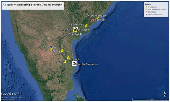
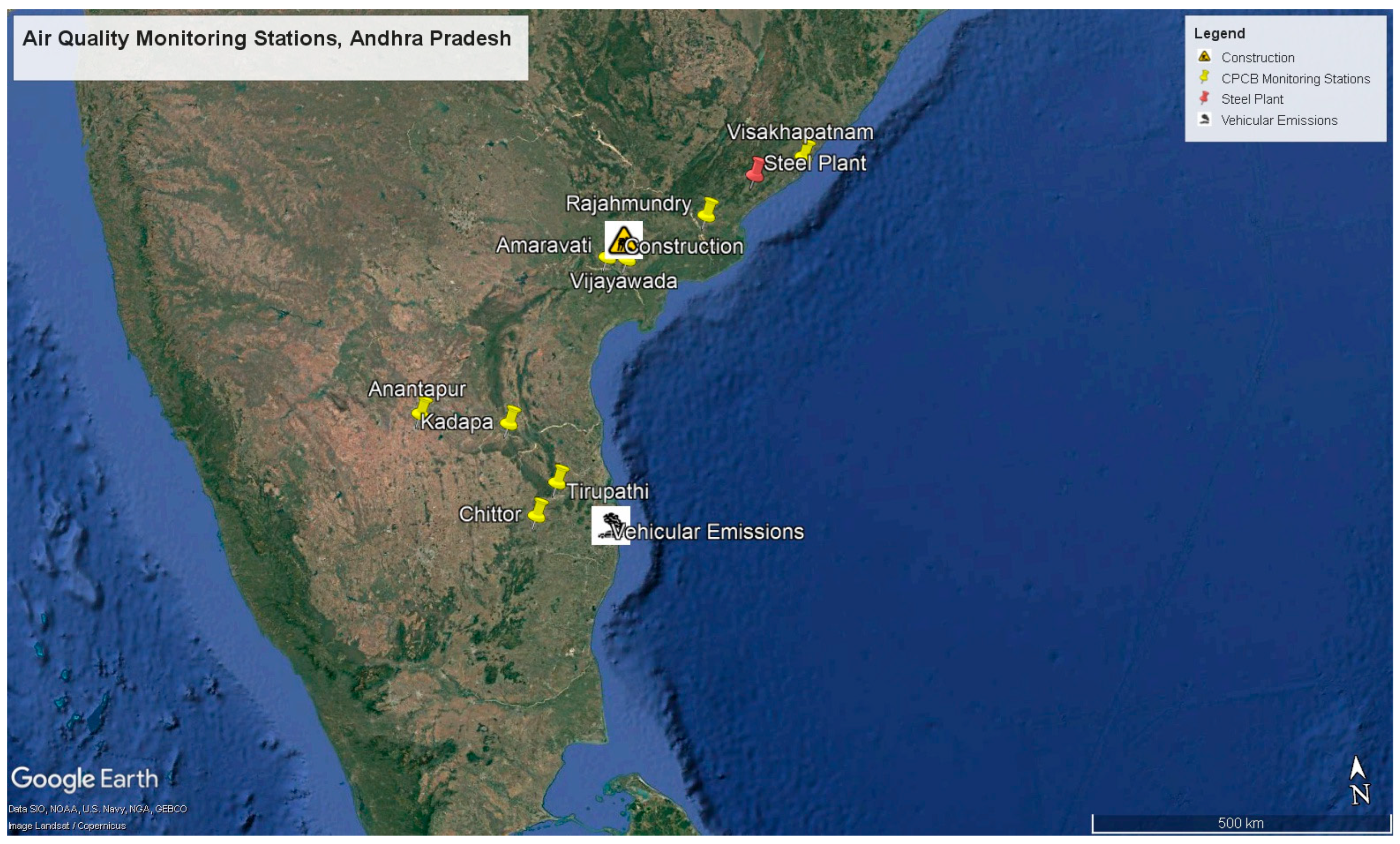
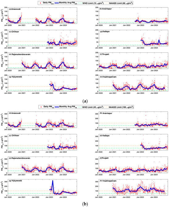
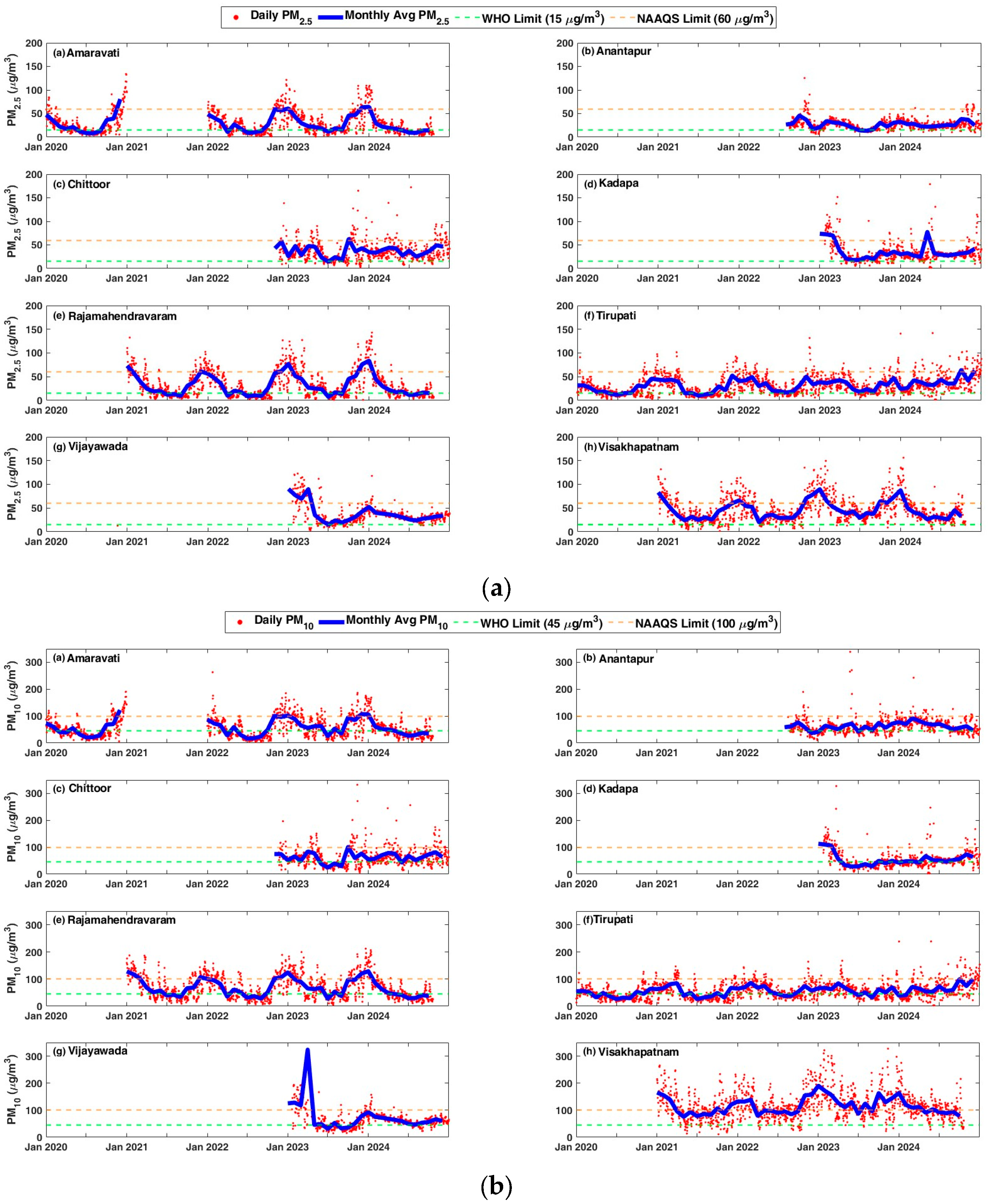
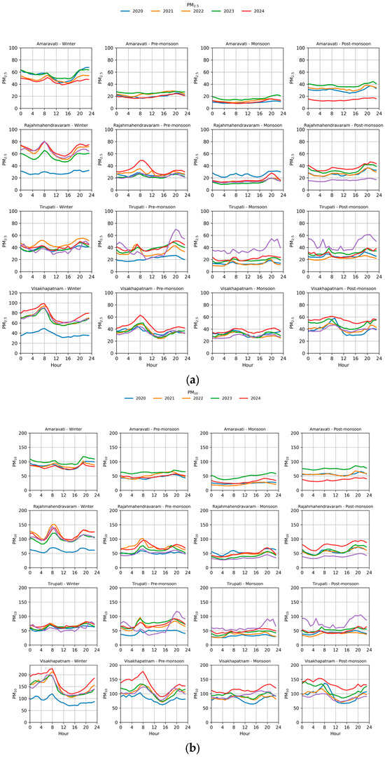
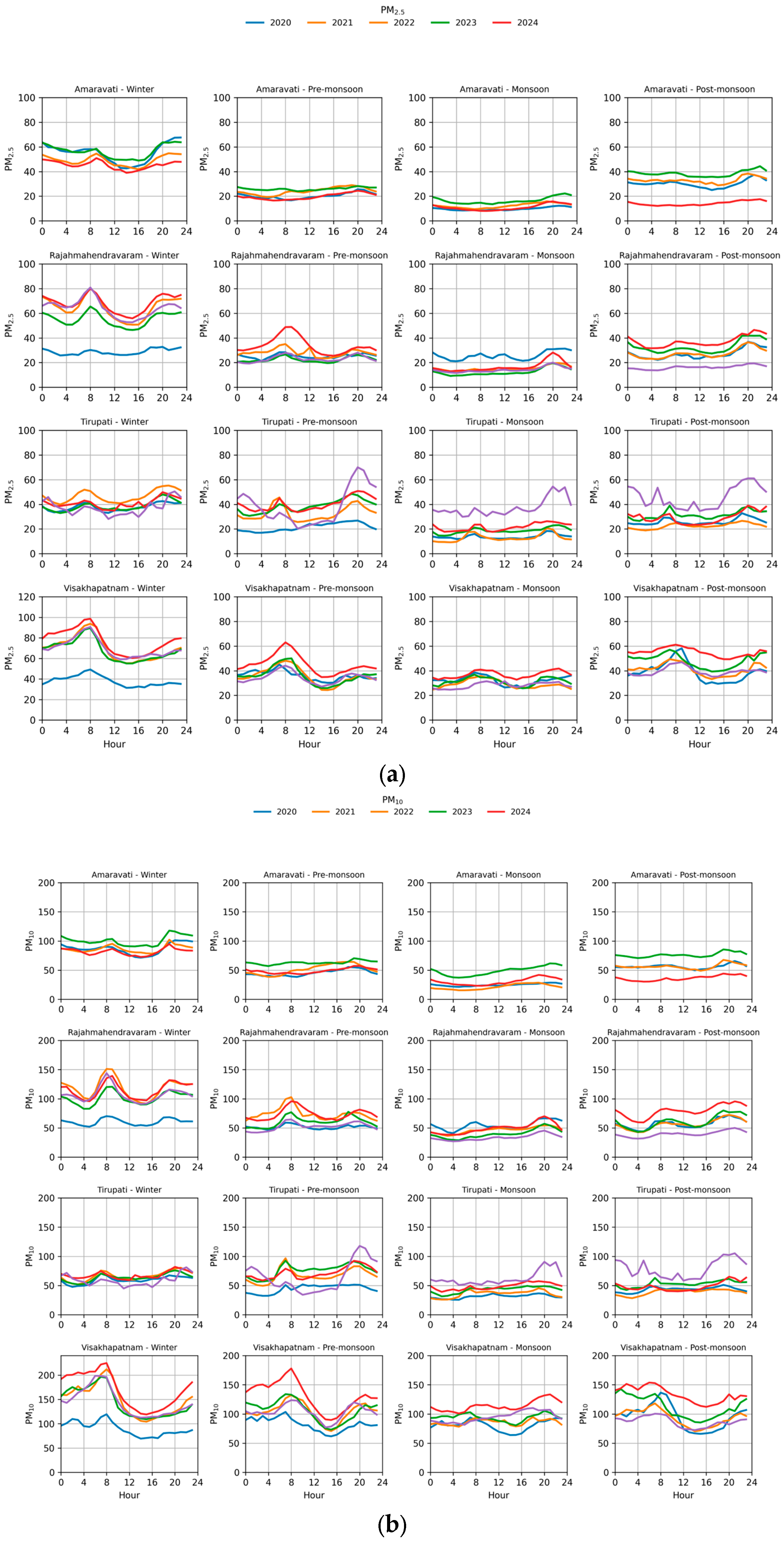
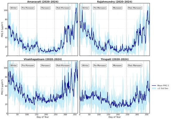
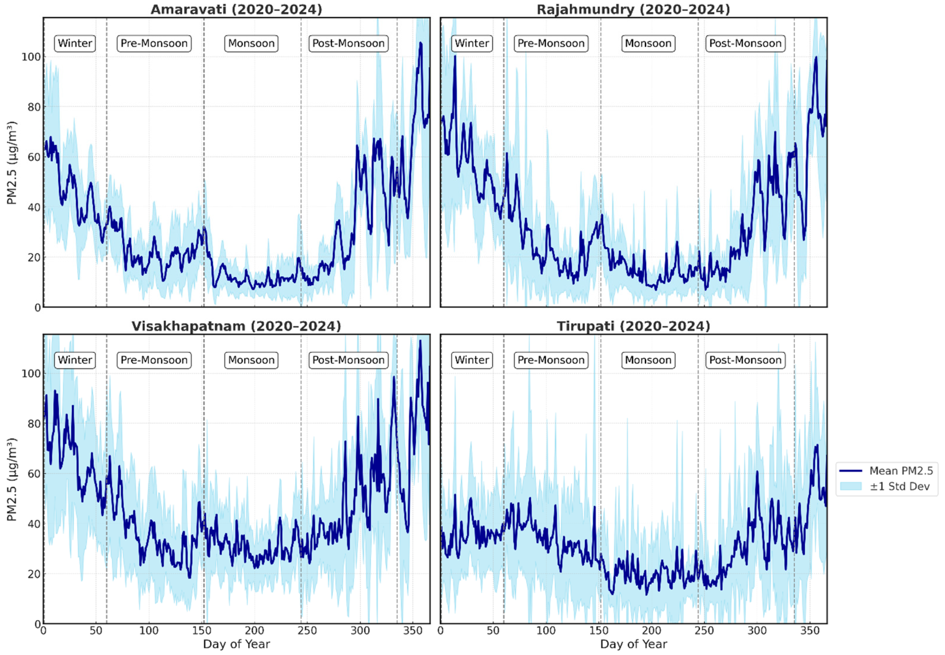
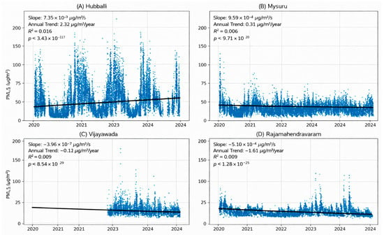
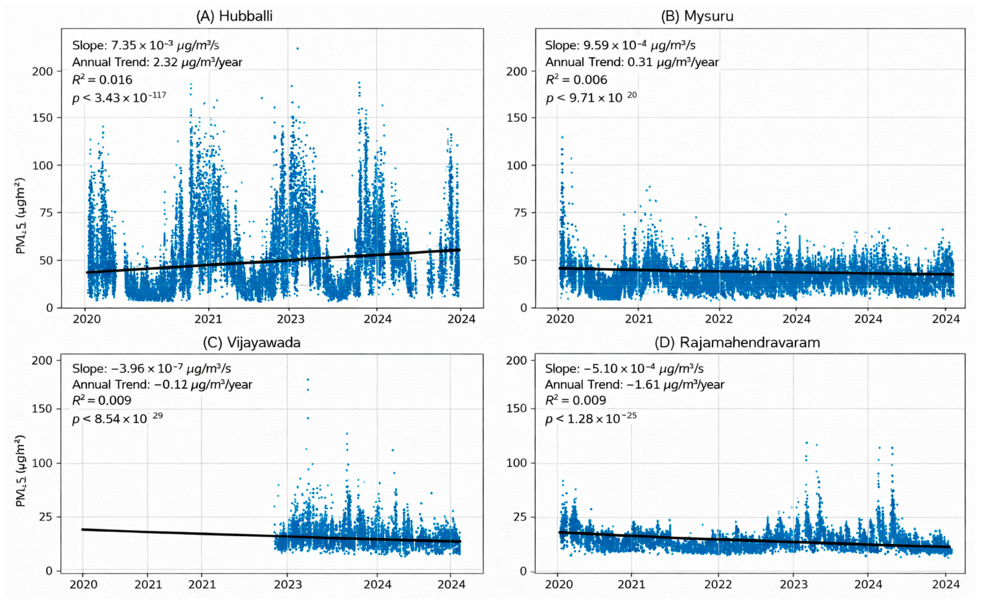
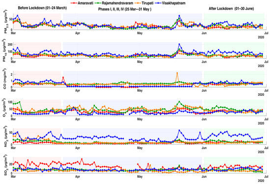
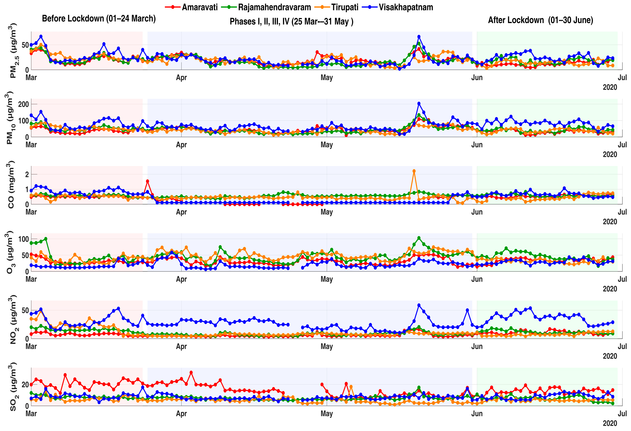
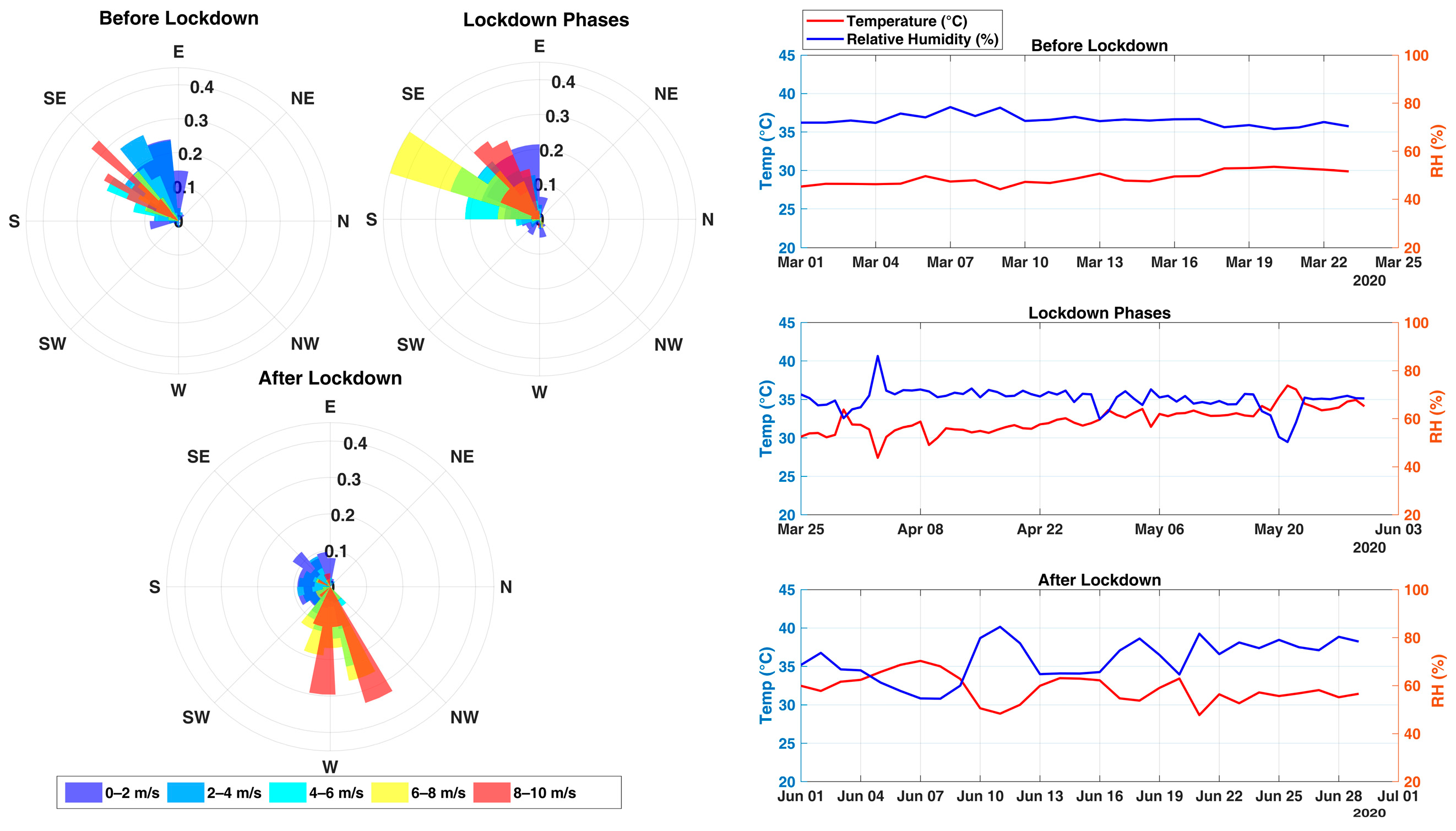
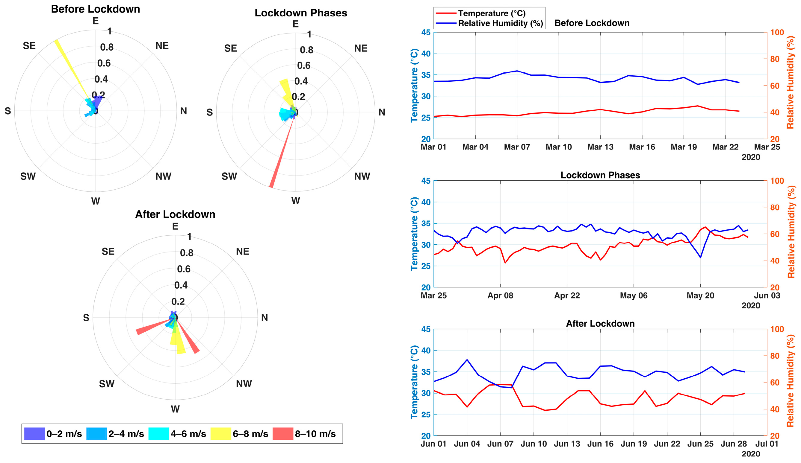
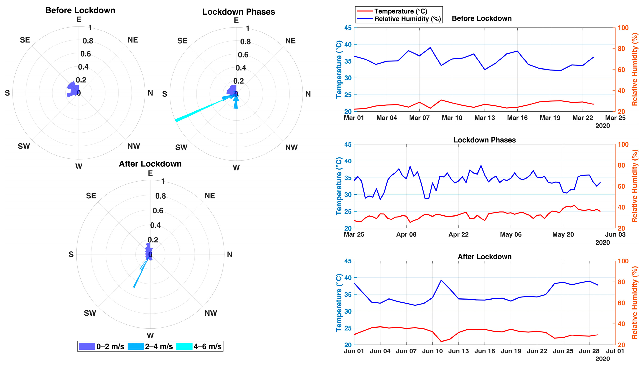
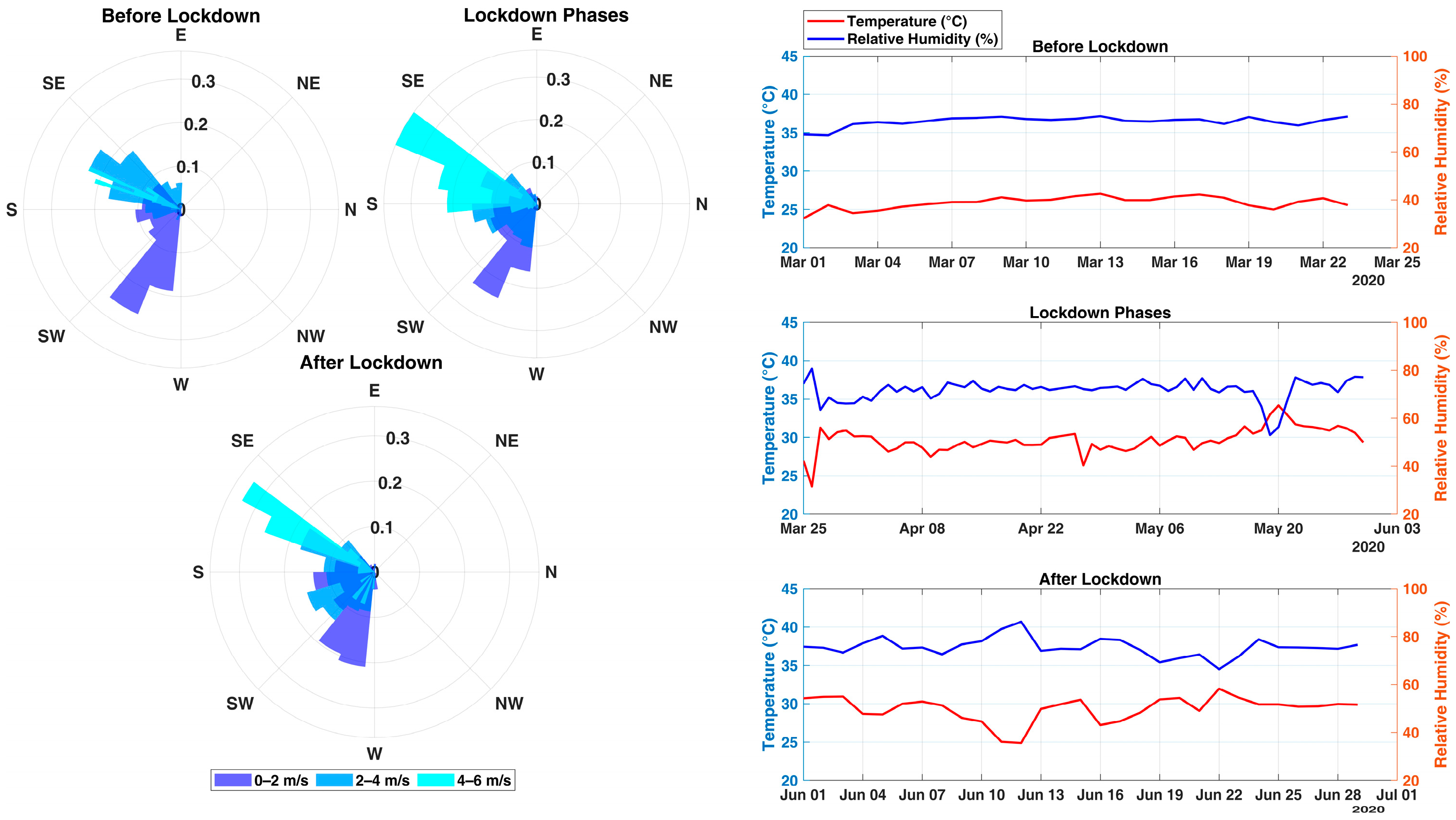
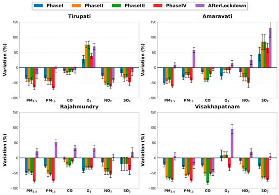
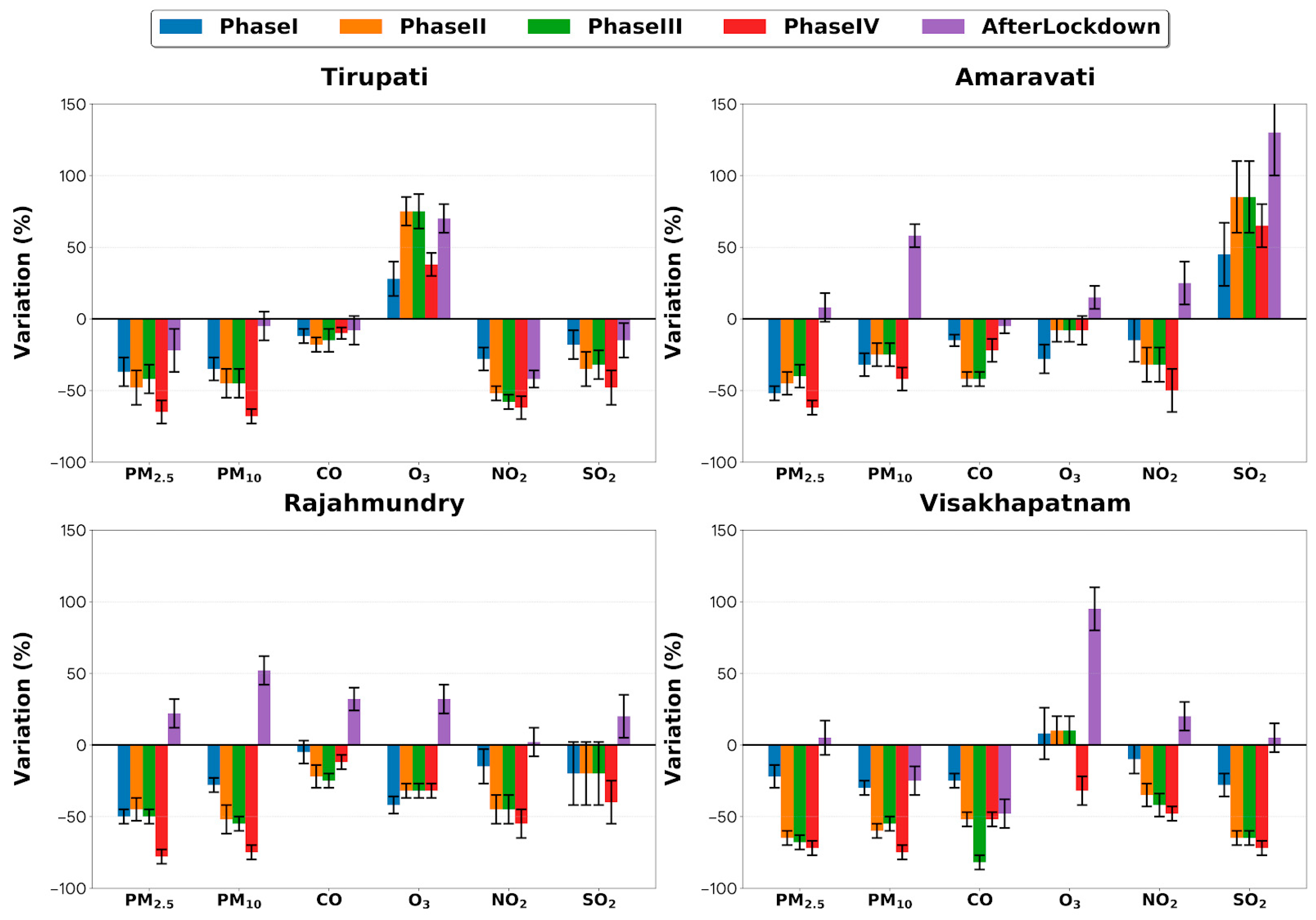
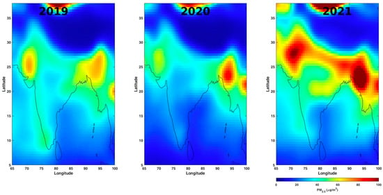
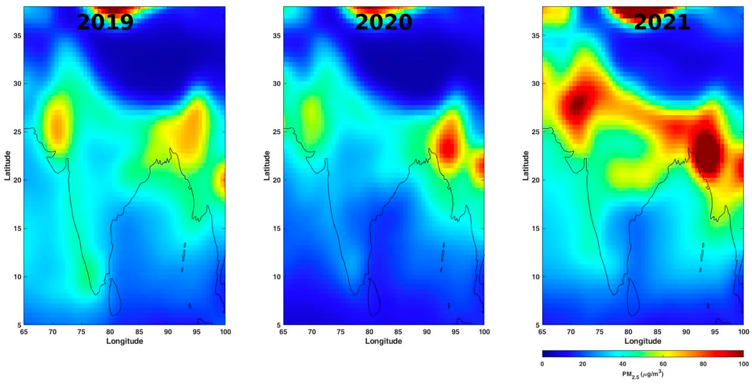

Disclaimer/Publisher’s Note: The statements, opinions and data contained in all publications are solely those of the individual author(s) and contributor(s) and not of MDPI and/or the editor(s). MDPI and/or the editor(s) disclaim responsibility for any injury to people or property resulting from any ideas, methods, instructions or products referred to in the content. |
© 2026 by the authors. Licensee MDPI, Basel, Switzerland. This article is an open access article distributed under the terms and conditions of the Creative Commons Attribution (CC BY) license.