


Abstract
In the context of intensifying climate change, understanding the spatial heterogeneity of urban climate risk is critical to effective climate governance in the United States. This study takes 251 major Metropolitan Statistical Areas (MSAs) in the United States as the analytical unit and establishes a multidimensional urban climate risk assessment framework covering hazard risk, exposure vulnerability, and adaptive capacity. Principal Component Analysis (PCA) is adopted for dimensionality reduction to extract key factors, and K-means clustering is used to identify the spatial differentiation characteristics of climate risk across these MSAs. The results show that climate risk in U.S. MSAs presents significant spatial disparities and can be categorized into four types: high resource and adaptive capacity, high exposure with insufficient adaptive support, complex socio-environmental vulnerability, and low current vulnerability with latent cumulative risk. Based on these findings, this study proposes targeted policy recommendations, including promoting inter-MSA coordination and adaptive capacity spillover, implementing gray–green integrated infrastructure development and enhancing social resilience in the southeastern coastal regions, strengthening equity orientation in climate governance, and advancing proactive governance of cumulative and chronic risks. These conclusions provide a reference for relevant authorities to formulate climate policies.
1. Introduction
Since the advent of the 21st century, climate change has emerged as one of the most severe, urgent, and long-term existential threats confronting humanity [1,2,3], which is causing substantial damage to both natural and anthropogenic systems upon which human survival depends. Temperature records across all continents are being repeatedly broken, and economic losses caused by extreme weather events surged by 23% between the periods of 2010–2014 and 2018–2022 [4]. Cities, featuring concentrated demographic aggregation and hosting a multitude of infrastructure and services critical to human well-being, are particularly vulnerable to risks [5,6]. Global warming itself elevates urban temperatures, where urban heat island phenomena further intensify such impacts, along with aerosol radiative forcing [7]. Concomitant severe convection, extreme downpours, heatwaves, haze, and diseases exert a detrimental impact on the ecological stability and livability of cities. Against this backdrop, understanding the spatial heterogeneity of climate risks has become a critical prerequisite for effective climate governance and, in turn, for advancing urban sustainable development.
In its Sixth Assessment Report (AR6), the Intergovernmental Panel on Climate Change (IPCC) states that climate risk arises from the interaction of hazards, exposure, and vulnerability. It emphasizes that risk is determined not only by natural climatic factors but also by socioeconomic conditions and spatial patterns of development. This comprehensive perspective establishes a solid theoretical foundation for the comparative assessment of large-scale climate risks, and enables a more precise delineation of the theoretical boundaries and analytical dimensions of urban climate risk research. Meanwhile, a substantial body of empirical research has emerged around urban climate risk and related issues. Such studies commonly employ technical approaches including principal component analysis (PCA) or factor analysis (FA) [8,9,10,11], and multi-criteria decision-making (MCDM) methods (e.g., AHP, TOPSIS, VIKOR) [10,12,13], as well as machine learning (ML) and deep learning (DL) [14,15,16], to identify, measure and compare urban risk levels, vulnerability characteristics, and adaptive and governance capacities. Building on these foundations, the scope of relevant research has continued to expand, gradually coalescing into several well-defined thematic clusters. These primarily include vulnerability assessment and the development of risk indicator systems [10,11,13,16,17,18,19,20], urban climate change governance and the formulation of policy frameworks [21,22,23,24,25,26,27], nature-based solutions (NbSs) to addressing climate risks [28,29,30,31,32,33,34,35], urban heat risk [20,36,37,38,39,40], the principles of equity and justice in risk governance [41,42,43,44,45,46], risk identification and decision-making supported by digital and intelligent technologies [15,16,34,47,48,49,50], and studies centered on enhancing urban climate resilience and adaptive capacity [51,52,53,54,55,56,57,58].
Meanwhile, a growing body of research has recognized that urban climatic risk is not a simple superposition of individual indicators, but a complex systemic outcome co-shaped by multiple socio-environmental processes [59,60,61,62]. Specifically, the hazard dimension is primarily shaped by changes in the frequency and intensity of climate events, including extreme heat, heavy rainfall, flooding and drought under climate change, and thus exhibits a strong natural attribute [62,63,64]. Exposure is closely associated with the spatial agglomeration of population and assets, land use change, urban expansion and built environment patterns [63,64,65]. It reflects the sensitivity of human activities and urban spatial organization to climate perturbations. Vulnerability is further rooted in disparities across socioeconomic structures, including income inequality, demographic age differences, the coverage and accessibility of public services, infrastructure completeness, and governance capacity, which reflects variations in the ability of different regions to resist and withstand climate shocks [66,67,68,69]. Furthermore, the three aforementioned dimensions are not isolated [62]; instead, they are intercoupled via land development, industrial layout, population mobility, resource–capital allocation, and policy governance, and jointly generate the spatial heterogeneity of urban climate risks [70,71]. For instance, rapid urban expansion and industrial agglomeration may further concentrate population and assets in high-risk areas, thereby increasing regional exposure [72,73,74]. Meanwhile, socioeconomic inequality can significantly widen disparities in vulnerability across regions under similar disaster risk conditions [69]. Moreover, differences in infrastructure development, ecological conservation, and public governance capacity further alter the formation mechanism and spatial distribution pattern of urban climate risks by shaping risk buffering, resource allocation, and emergency response processes [62,75,76,77,78]. It follows that the spatial differentiation of urban climate risks is, in essence, a joint outcome of disparities in natural climatic conditions, urban spatial development, and socioeconomic structures. Accordingly, constructing an indicator system based on the functional and interactive mechanisms of hazard, exposure, and vulnerability enables a more accurate identification of the formation logic and spatial variations in urban climate risks.
Although existing research has yielded substantial achievements in methodological applications, thematic expansion, and mechanism identification, it still exhibits several limitations in the empirical analysis and spatial comparison of urban climate risks. First, existing studies have mostly been conducted at the individual city or regional level [9,10,13,14,15,17,22,47,79,80,81,82,83], and systematic comparative analyses of urban climate resilience at the national scale remain relatively insufficient. Second, most existing studies focus on constructing composite indices to rank urban climate risks or adaptive capacities [18,19,44,47,49,53,62,84,85,86,87]. Nevertheless, such methods may obscure the dynamic interactions and spatial heterogeneity across different dimensions [88]. They may also generate misleading and ambiguous ranking outcomes due to weight sensitivity, information loss, and compensatory effects [89], where minor adjustments to indicator weights can alter priority sequences, and statistical units with divergent domain scores may be grouped together owing to similar aggregate values. As a result, these methods can hardly support differentiated governance strategies for regions exposed to distinct types of climate risks. Third, within the U.S. context, most existing studies on urban climate risk use states, cities, and counties as units of analysis [23,24,53,54,90], while relatively few studies have been conducted from the perspective of metropolitan statistical areas (MSAs). While the former represents a statutory U.S. administrative unit with more readily available data, it cannot reflect the spatial continuity of climate risks or their socioeconomic interconnectedness as effectively as the latter. On the one hand, urban climate risks are often cross-jurisdictional, systemic, and holistic, and are not constrained by administrative boundaries [90,91,92,93,94]. Conventional administrative units such as states, counties, and cities tend to disrupt the socioeconomic and physical continuity of climate risks, resulting in fragmented assessments that can hardly support regional coordinated adaptation. On the other hand, as functional regions delineated on the basis of commuting ties and economic interactions [95], MSAs can more authentically reflect the spatial organization and internal linkage mechanisms of urban systems. Compared with traditional administrative units, MSAs not only encompass urban core areas and their surrounding commuting zones but also integrate critical elements such as population mobility, industrial linkages, and infrastructure networks [96]. They align better with the actual spatial extent of climate risks in the multi-dimensional coupling process of “hazards–exposure–vulnerability”, and are thus widely regarded as the most appropriate scale for analyzing urban sustainability and climate risk governance [97].
To address these gaps, this study examines 251 major metropolitan statistical areas (MSAs) in the United States. We establish an urban climate risk assessment indicator system within the hazard–exposure–vulnerability framework, and employ principal component analysis (PCA) combined with K-means clustering to identify the spatial differentiation and typological structure of urban climate risks across U.S. cities. This paper aims to address the following research questions: (1) Is there significant spatial heterogeneity in climate risk across U.S. metropolitan statistical areas? (2) How do hazard, exposure, and vulnerability collectively shape the spatial pattern of urban climate risk? (3) Compared with traditional comprehensive ranking methods, can typological classification more effectively reveal the structural differences in urban climate risk?
The contributions of this paper are threefold: First, by adopting metropolitan statistical areas (MSAs) as the functional urban analytical units, this study complements existing research on cross-city comparisons of climate risk at the national scale in the United States. Second, within the hazard–exposure–vulnerability framework underpinned by IPCC AR6, we establish a multidimensional indicator system that strengthens the theoretical relevance of indicator selection. Third, by identifying spatial heterogeneity in urban climate risk through a typological approach rather than simple ranking, this paper provides more robust empirical support for differentiated and targeted governance of urban climate risk.
2. Materials and Methods
2.1. Research Area
This study takes metropolitan statistical areas in the United States as its analytical units. Considering the notable differences in spatial coverage, statistical caliber, and data completeness among various data sources, especially the extensive missing values for certain smaller or remotely located regions, this study finally selects 251 major metropolitan statistical areas with relatively complete data as research samples (their details are provided in Table A1 in Appendix A). These samples cover major population and economic centers in the United States, accounting for approximately 78% of the total U.S. population. They therefore provide a solid basis for identifying the overall spatial patterns of climate risk disparities across major metropolitan areas. Nevertheless, it should be clarified that this study does not aim to depict the full climate risk landscape across all U.S. metropolitan statistical areas. The findings are primarily generalizable to major metropolitan areas with relatively complete data. Smaller, more remote metropolitan areas or those with severe data limitations may still be underrepresented or omitted in this analysis.
The geospatial distribution of the select 251 MSAs is shown in Figure 1 below.
Figure 1.
The selected 251 MSAs in this research.
2.2. Data
2.2.1. Evaluation Indicator System
The evaluation indicator system of this study is primarily grounded in the core climate risk framework of IPCC AR6, which encompasses three dimensions: hazard, exposure, and vulnerability. To adequately capture the physical and social characteristics of urban systems exposed to climate hazards as well as their adaptive potential, this study further disaggregates vulnerability into sensitivity and adaptive capacity following the definition given in IPCC AR6, thereby expanding the climate resilience assessment framework into four primary indicators. The impacts of these four elements on climate risk are illustrated in Figure 2 below. Based on a comprehensive evaluation of four key dimensions, including theoretical relevance to the causal structure of climate risk, empirical evidence from prior urban climate risk research, comparability for cross-MSA analysis, and data availability and integrity, this study establishes 27 secondary indicators corresponding to four primary indicators. Details are provided in Table 1.
Figure 2.
Climate Risk Framework.
Table 1.
Indicator System for Climate Risk Assessment.
2.2.2. Data Sources and Benchmark Year
Data used in this study were obtained from the NASA Langley Research Center, the Federal Emergency Management Agency (FEMA), the U.S. Census Bureau, the University of Wisconsin Population Health Institute/Robert Wood Johnson Foundation, the USDA National Agricultural Statistics Service (NASS), and the U.S. Energy Information Administration (EIA), ensuring authenticity and reliability.
It should be noted that the benchmark years of the selected indicators are not fully identical. Rather than forcing all variables into a strictly synchronous annual framework, this study constructed a multi-temporal integrated dataset according to the statistical properties, update cycles, and availability of different indicators. Specifically, climate hazard and environmental exposure indicators mainly refer to 2023 so as to reflect the most recent risk environment, whereas socioeconomic and demographic indicators primarily rely on 2018–2022 ACS five-year estimates. This choice is methodologically justified because ACS five-year estimates are designed to provide more reliable and comparable measurements for smaller geographic units, even though they are less current than single-year estimates.
A small number of health-related and inequality-related variables were taken from the most recent available release versions, due to differences in official publication schedules and data production cycles across sources. County Health Rankings, for example, explicitly compiles its annual release from multiple national and state datasets and uses the most recently available data for nearly all counties, while also acknowledging that measure availability is constrained by geographic, source, and time limitations. From the perspective of climate risk assessment, this temporal design matches relatively stable structural vulnerability with more temporally volatile contemporary hazard exposure, rather than treating all indicators as if they represented a perfectly time-synchronous annual snapshot. Because the purpose of this study is to identify relative climate risk differentiation and typological patterns across metropolitan areas, rather than to estimate the exact risk state of a single year, such a multi-temporal data design was considered methodologically appropriate for the present comparative analysis.
The source and time period of each indicator are detailed in Table 2 below.
Table 2.
Data Sources and Statistical Periods.
2.2.3. Data Processing
To ensure the consistency, comparability, and representativeness of data across the 251 MSAs, this study adopts specific aggregation and processing methods to unify all raw data to the MSA level according to the source characteristics and spatial granularity of the original datasets.
For the NASA POWER climate indicators, this study extracted daily data for 2023 based on the geographic centroid coordinates of each MSA and further calculated annual statistical values (e.g., the annual average dimension refers to the arithmetic mean of the annual maximum and minimum temperatures, while the number of extreme high-temperature days is defined as days with a daily maximum temperature exceeding 35 °C). This centroid-based approach is adopted mainly because the research objective is to identify the overall spatial pattern and typological differences in climate risk across MSAs, rather than to examine fine-grained variations within individual metropolitan areas. Moreover, this method ensures consistency and comparability in climate data extraction for the 251 MSAs at the national scale. For the FEMA National Risk Index (NRI) risk scores, the standardized county-level values (ranging from 0 to 100) are aggregated to the MSA level through simple arithmetic averaging, which equally reflects the overall risk level of all counties within each MSA. Furthermore, the 5-year rolling data (2018–2022) from the U.S. Census Bureau are aggregated from the county level to the MSA level using a population-weighted average method. Specifically, county-level indicators are weighted by resident population and summed, and then divided by the total population of the corresponding MSA. This approach reduces areal interference and reflects the characteristics of population agglomeration. Two indicators retrieved from the University of Wisconsin Population Health Institute are aggregated into MSA-level values by extracting the corresponding county-level observations within each MSA and calculating their medians, thereby mitigating the influence of extreme outliers. Meanwhile, for the three land-cover indicators obtained from the NASS, the area of the target land category in each county within an MSA is summed up and then divided by the total natural land area of the MSA and multiplied by 100%. The total natural land area is defined as the sum of forest, wetland, grassland, woodland, shrubland, and open water areas. Finally, regarding the renewable energy proportion indicator from the EIA, this study first extracts records of all power generation units and aggregates them to the county level. Subsequently, the county-level data are summed up to obtain MSA-level values. The proportion is quantified by dividing the aggregate installed renewable energy capacity within the MSA by the overall installed capacity, followed by percentage conversion.
2.2.4. Correlation Analysis
To explore the correlations among the selected 27 indicators and assess potential multicollinearity issues, this study constructed a Pearson correlation matrix and presented it in the form of a heatmap (Figure 3).
Figure 3.
Heatmap of the Pearson Correlation Matrix for the Climate Risk Assessment Indicator System.
Correlation analysis revealed that the overall correlation level among the 27 selected indicators was low (mean r = 0.075). However, pairs of indicators with significant correlations accounted for 61.8%, indicating no severe multicollinearity among the variables while demonstrating certain structural associations. From the perspective of individual dimensions, the indicators within the Sensitivity category exhibit the highest internal correlation, with a mean r value of 0.419, indicating relatively pronounced coupling. The Hazard category yields a mean r of 0.178, suggesting weak correlations and reflecting a certain spatial consistency in the distribution of climatic stressors. By contrast, Exposure and Adaptive Capacity show the lowest internal correlations, implying relatively discrete indicator characteristics. From a cross-dimensional perspective, the Hazard indicators show a moderate positive correlation with the Sensitivity indicators (mean r = 0.236), reflecting the coupling between natural risk and social vulnerability.
In summary, the indicator system exhibits the characteristic of weak overall correlation with strong local coupling. Therefore, Principal Component Analysis (PCA) is adopted for dimensionality reduction alongside noise elimination to extract core structural information, and enhance the reliability of subsequent K-means clustering.
2.3. Methodology
2.3.1. Principal Component Analysis (PCA)
Principal Component Analysis (PCA) is a classic unsupervised linear dimensionality reduction method that can reduce the dimensionality of a dataset while retaining as much information of the original dataset as possible [106,107]. Its core idea is to transform the correlated variables in the original high-dimensional feature space into a small number of uncorrelated comprehensive variables via orthogonal transformation, and these comprehensive variables are referred to as principal components. Owing to its effectiveness in dimensionality reduction and redundancy elimination for high-dimensional data, as well as its ability to avoid the “curse of dimensionality”, PCA has been widely applied in multiple linear regression, the detection of data structures capable of accounting for the most significant data variances, and clustering analytical approaches [108].
Its specific implementation processes are as follows.
- Data Standardization
To eliminate the impact of different dimensions and scales among various features, and ensure that PCA extracts principal components based on the variance structure of the data rather than dimensional differences, it is necessary to perform Z-score standardization on the data prior to analysis.
Here, and represent the per-feature mean and standard deviation vectors, ensuring the standardized data satisfied E () = 0, and the variance of each dimension equals 1.
- 2.
- Calculation of the Covariance Matrix
After Standardization, compute the covariance matrix of the data as follows.
The covariance matrix reflects the linear correlation between different features, and the goal of PCA is just to eliminate this correlation via orthogonal transformation.
- 3.
- Eigenvalue Decomposition
Eigenvalue decomposition is conducted on the covariance matrix:
where devotes the i-th eigenvalue (satisfying ), and is the corresponding unit eigenvector. Each eigenvector. Each eigenvector defines a principal component direction, with quantifying the data variance along this direction.
- 4.
- Selection of Principal Components
The eigenvectors associated with the largest eigenvalues are selected to construct the projection matrix , where . The number of principal components is typically determined by the Cumulative Proportion of Variance ():
For , the reasonable threshold is usually between 70% and 90%, and it should be adjusted according to the actual situation of the dataset [109,110]. Another important criterion is the Kaiser criterion, whose core idea is to retain all principal components with eigenvalues greater than 1 [111].
- 5.
- Data Projection
Finally, the original dataset is projected onto the selected k-dimensioned principal component space, yielding the reduced-dimensional representation.
Each row of the matrix corresponds to the new feature vector of the corresponding sample in the principal component coordinate system. The dimensions are mutually orthogonal and arranged in descending order of information content.
2.3.2. K-Means Clustering
After performing PCA and obtaining the low-dimensional representation Z, the paper applies the K-means clustering algorithm to partition the samples into unsupervised groups. As a representative partitioning clustering technique, K-means endeavors to split data points into K non-overlapping groups, such that intra-cluster samples exhibit maximum similarity and inter-cluster samples demonstrate maximum dissimilarity.
Formally, let the dimensionally reduced data be , where represents the coordinates of the i-th sample in the principal component space. K-means attempts to solve the following optimization problem:
where denotes the set of samples belonging to the -th cluster, is the centroid of that cluster, and typically denotes the Euclidean norm.
This paper combines PCA with K-means clustering. Specifically, PCA is first employed to eliminate data redundancy and noise as well as reduce dimensionality. On this basis, K-means clustering is then applied to achieve efficient and accurate group partitioning, which resolves the challenge of diminished K-means performance encountered in the analysis of sparse high-dimensional data [112].
The principal component analysis and K-means clustering in this study were conducted using SPSS 27.0 and Python 3.14, respectively. Furthermore, it should be noted that DeepSeek v3.2 was adopted to assist with code revision and optimization, image generation and editing, as well as partial textual polishing throughout the research. All content generated with the auxiliary support of DeepSeek v3.2 has been fully reviewed and verified for accuracy and rationality.
3. Results and Discussions
3.1. Results of Principal Component Analysis
3.1.1. Kaiser-Meyer-Olkin (KMO) and Bartlett’s Test of Sphericity
The study employs SPSS 27.0 for principal component analysis. All indicators are standardized using the Z-score method to eliminate dimensional discrepancies and scale differences prior to analysis. Notably, this study retains the original directional interpretation of all variables and does not implement uniform reverse coding prior to standardization. This specification is adopted because the present study uses principal component analysis to extract the latent covariance structure among variables, rather than to construct a single additive risk index. Therefore, retaining the original directions of the variables does not compromise the mathematical validity of the principal component analysis procedure. Meanwhile, the directional properties of the indicators are fully considered when interpreting the component loadings and assigning names to the extracted principal components in subsequent steps.
After conducting Z-score standardization on the data of 27 indicators in the selected indicator system, the Kaiser-Meyer-Olkin (KMO) and Bartlett’s Test of Sphericity were performed to verify whether the data were suitable for principal component analysis.
As presented in Table 3, the KMO value is 0.743, which exceeds the recommended threshold of 0.6 for conducting principal component analysis (PCA) [113]. Furthermore, Bartlett’s test of sphericity yields a p-value of less than 0.001, demonstrating that the data are appropriately structured for principal component analysis [114].
Table 3.
KMO and Bartlett’s Test of Sphericity.
3.1.2. Extraction of Principal Components
Principal components are extracted from the indicator data. Table 2 below is the variance explanation rate table, which represents the proportion of the variance of the original variables that each principal component can explain, and it acts as a core metric for measuring the amount of retained information [115].
Table 4 indicates that the initial seven principal components each possess eigenvalues exceeding unity, satisfying the Kaiser criterion; thus, these principal components are extracted for subsequent analysis. The cumulative variance explained by these principal components reaches 74.453%, indicating that they retain more than 70% of the information in the original data. This indicator falls within the acceptable range in academic circles, especially in the field of humanities and social sciences [116,117].
Table 4.
The variance explained rate of principal components.
3.1.3. Component Loading Analysis
In academic terms, principal components simply represent weighted linear syntheses of the initial indicators and lack clear practical interpretation [109]. Only through component loading analysis can we identify how observed variables map to latent variables (e.g., a comprehensive evaluation index) [118], recognize the correlation patterns among variables [119], and assess the quality of data compression [120]. In short, loading analysis enables principal components to transform from abstract linear combinations into substantive concepts that can be used for decision-making [107,117].
As as shown in Table 5 below, the primary principal component (PC1) is predominantly characterized by substantial loadings across two distinct dimensions: socio-demographic susceptibility (encompassing the proportions of the minorities, overcrowded housing, and limited English proficiency) and climatic exposure (including annual mean temperature, solar radiation, and the frequency of extreme heat events). Consequently, PC1 is designated as the Socio-Environmental Composite Vulnerability Factor, reflecting the interplay between societal fragility and environmental stressors. In PC2, the items with high loadings are mainly socio-economic indicators associated with climate adaptability, including public transit usage rate, per capita income, homeownership rate, number of primary care physicians, and proportion of the uninsured population. Therefore, it is named the socio-economic adaptability factor. Furthermore, driven by high loadings on natural ecological resources, precipitation-related hazards, and population vulnerability metrics, PC3 is conceptualized as the ‘Ecological Regulation, Pluvial Hazard, and Demographic Sensitivity Factor. PC4 integrates natural and social indicators—including forest cover and economic demographics—with wildfire and loss risk scores, thus being designated as the ‘Natural-Social Asset Exposure and Disaster Loss Risk Factor.
Table 5.
The Loading Matrix.
Regarding PC5, its loadings are primarily concentrated on the share of public transit and the share of renewable energy, with opposing polarities. Consequently, it is designated as the “Public Transit–Green Energy Structural Mismatch Factor,” reflecting the spatial inconsistency between these two dimensions of urban sustainability. As for PC6, given its high loadings on cold wave risk, river flood risk, and the proportion of car-free households, it can be designated as the Cold-Flood Hazard and Mobility-Related Sensitivity Factor. The interpretation of PC7 is more straightforward, with significant loadings concentrated predominantly on the proportion of wetlands. Accordingly, it is designated as the “Wetland Ecological Regulation Factor,” representing the specialized role of wetland ecosystems in providing natural buffering and environmental regulation.
3.2. Results of K-Means Clustering Analysis
3.2.1. Selection of the Optimal Number of Clusters (K)
Before performing K-means clustering, selecting and determining the optimal value of K is of paramount importance, as it directly dictates the quality and validity of the resulting clusters [121]. To ensure a robust identification of the optimal K-value, a multi-criteria validation framework was adopted, synthesizing results from the Elbow method alongside internal validity indices such as the Silhouette coefficient [122,123], Calinski–Harabasz (CH) index [124,125,126], and Davies-Bouldin (DB) index [127,128].
The cluster analysis was implemented in Python 3.14 using the scikit-learn library, with the seven principal component scores derived from PCA as input variables. Candidate solutions with cluster numbers ranging from 2 to 10 were evaluated sequentially. The model explicitly set “random_state = 42” to ensure reproducibility and “n_init = 10” to mitigate the risk of local optima caused by random initial cluster center selection. All other parameters followed the program defaults. For each candidate cluster number, inertia, silhouette coefficient, Calinski–Harabasz index, and Davies–Bouldin index were calculated separately (as shown in Figure 4 below). The optimal cluster number was determined by combining these statistical metrics with the substantive interpretability of the clustering outcomes.
Figure 4.
The optimal K-value determination process.
As illustrated in Figure 4A, the inertia curve exhibits a distinct inflection point at K = 4, beyond which the slope begins to level off. This suggests that the marginal gain in error reduction diminishes as the number of clusters increases, identifying K = 4 as the ‘elbow point’ that achieves an optimal balance between model parsimony and explanatory power [121,129]. In the Silhouette Coefficient plot, the score for K = 4 represents the highest value excluding K = 2. Although the latter yields a superior absolute score, K = 4 remains the optimal choice when considering the balance between classification granularity and the fact that K = 4 is identified as the elbow point in the inertia curve. In Figure 4D, although the Davies-Bouldin (DB) index at K = 4 is not the global minimum, it represents the local optimum for K ≤ 5. Given that the disparity in DB scores between K = 4 and most higher cluster numbers (K = 6, 7, 10) is negligible, K = 4 is considered the most appropriate choice to avoid over-partitioning while maintaining statistical robustness. Lastly, in the CH index plot, although the value at K = 4 is significantly lower than those at K = 2 and 3, this does not alter the conclusion that K = 4 is the most appropriate choice. This decision is justified by the fact that K = 4 serves as a distinct elbow point in the CH curve and represents the second-highest peak for the Silhouette Coefficient. Furthermore, the DB index at K = 4 is substantially lower than that at K = 2 or 3, reinforcing the superiority of this partition through multi-metric convergence.
Therefore, the most appropriate K value is 4.
3.2.2. Implementation of K-Means Clustering
The PCA-reduced data were partitioned using the K-means clustering, as shown below. Table 6 and Figure 5 delineate the cluster centroids, representing the average scores of each cluster across the seven principal components (PCs).
Table 6.
Mean scores of each cluster across the seven principal components.
Figure 5.
Comparison of cluster centroid scores across the seven principal components.
Based on the aforementioned mean score data, the distinctive characteristics of each cluster can be clearly identified.
- Cluster 1 (High-Resource, High-Adaptive Capacity Type)
Cluster 1 comprises 22 metropolitan areas, accounting for 8.8% of the full sample. Its most distinctive feature is an exceptionally high mean value of 3.9709 on PC2, far exceeding that of all other clusters. This pattern indicates that the defining trait of this group is not an absence of climate risk, but rather strong socioeconomic resources, physical infrastructure, and service capacity. Meanwhile, positive values on PC1 (1.0177), PC3 (0.7665), and PC4 (0.3293) show that these regions still face moderate environmental and social pressures, yet possess greater adaptive capacity to manage such risks relative to other types. This group is therefore best characterized as high-resource, high-adaptive capacity areas, rather than simply low-risk or high-resilience regions. Representative metropolitan statistical areas (MSAs) include New York–Newark–Jersey City, Los Angeles–Long Beach–Anaheim, and Chicago–Naperville–Elgin. These highly developed regions typically maintain strong fiscal foundations, mature infrastructure networks, and comprehensive public services, which support robust disaster recovery and long-term climate adaptation.
- 2.
- Cluster 2 (High-Exposure, Insufficient Adaptive Support Type)
Cluster 2 includes 61 metropolitan areas, representing 24.3% of the sample. This type is distinguished by the highest score on PC3 (1.5226), a positive value on PC4 (0.3867), and a notably low value on PC2 (−1.3833). This profile reveals a core structural condition: elevated exposure to ecological and precipitation-related hazards and high concentrations of human and built assets, paired with relatively weak socioeconomic adaptive support. Although the score on PC1 (1.3985) indicates above-average social-environmental vulnerability, the critical issue for this type is not extreme social disadvantage, but a pronounced mismatch between high exposure and limited adaptive capacity. This group is accordingly classified as high-exposure, insufficient adaptive support areas. Representative MSAs include Miami, Tampa, and New Orleans, which exemplify the “Sunbelt dilemma”: rapid urban expansion, coastal development, and capital accumulation have outpaced investments in ecological protection and adaptive systems, leaving these regions particularly vulnerable to storm surges, flooding, and compound climate hazards.
- 3.
- Cluster 3 (Integrated Social-Environmental Vulnerability Type)
Cluster 3 accounts for 11.6% of the sample and represents the most vulnerable metropolitan type identified in this study. Its key feature is an extremely high mean value of 5.3193 on PC1, the most extreme deviation among all cluster centers. Negative values on PC3 (−1.2738), PC4 (−0.7255), and PC5 (−0.4949) indicate that risk in this group is driven not primarily by hazard exposure or asset concentration, but by overlapping environmental stress and deep socioeconomic vulnerability. Specifically, these MSAs are characterized by high poverty rates, inadequate public services, unstable employment, and scarce adaptive resources, all of which amplify the impacts of droughts, floods, and heat stress. This group is best labeled as integrated social-environmental vulnerability areas. Representative cases include McAllen–Edinburg–Mission and Brownsville–Harlingen, Texas, which illustrate a typical pattern where socioeconomic marginalization strongly exacerbates escalating climate risks.
- 4.
- Cluster 4 (Low Current Vulnerability, Latent Cumulative Risk Type)
Cluster 4 is the largest group, with 139 MSAs, representing 55.4% of the sample. Its primary characteristic is the lowest mean value on PC1 (−1.8846), with other components close to the sample average. This indicates no extreme social-environmental vulnerability or acute hazard exposure at present. However, this relatively balanced profile does not imply long-term safety; instead, it signals low current vulnerability but the potential for gradual accumulation of latent, slow-onset risks over time. This group is therefore identified as low current vulnerability, latent cumulative risk areas. Spatially, these MSAs are concentrated in the inland Northeast, the Great Lakes region, and the Great Plains, including Pittsburgh, Buffalo, Omaha, and Des Moines. These areas lack the strong fiscal and infrastructure advantages of Cluster 1 but avoid the intense coastal hazard pressures of Cluster 2. Their risk profile is best understood as stable in the near term, but subject to growing cumulative risks over time.
3.2.3. Visual Validation
To evaluate the robustness and empirical validity of the PCA-K-means clustering results, this study mapped the 251 MSAs onto a geographical coordinate system based on their respective climate risk typologies (Figure 5) for further visual validation. As illustrated in Figure 6, the visualization results account for significant spatial autocorrelation and patterns of regional clustering.
Figure 6.
Geographical Distribution of Climate Risk Clusters in the selected 251 MSAs.
- Cluster 1 (Green dots):
MSAs in this cluster are primarily concentrated in the Northeast Megalopolis and the West Coast Metropolitan Belt, the two most economically advanced regions in the United States. Characterized by abundant socio-economic resources, these areas exhibit robust climate adaptive capacity.
- Cluster 2 (Orange dots):
MSAs in this cluster are predominantly distributed across the Southeastern United States, specifically along the Gulf of Mexico and the Atlantic coasts. This region has historically been among the most severely threatened by climate-related hazards in the nation, facing significant risks from hurricanes, storm surges, and pluvial flooding [130,131,132,133,134,135], which defines its distinct “high exposure” profile.
- Cluster 3 (Red dots):
MSAs in Cluster 3 (Red dots) are primarily concentrated in California’s Central Valley, along the U.S.-Mexico border, and throughout the Deep South. These regions are characterized by per capita income levels that generally lag behind the national average, coupled with high unemployment rates, large immigrant populations, complex social structures, and unstable employment frameworks, alongside underdeveloped public infrastructure [136,137]. Furthermore, these areas frequently experience heatwaves and extreme heat events [138], while facing significant risks from drought and wildfires [139]. This spatial pattern of socioeconomic disadvantage overlapped with environmental pressure is highly consistent with its extremely high score on PC1, which validates its classification as a complex social-environment vulnerability type and further strengthens the empirical rationality of the clustering results.
- Cluster 4 (Blue dots):
Cluster 4 (Blue dots) is densely distributed across the Great Lakes region, the inland Northeast, the Central and Northern Great Plains, and portions of the western interior plateaus. Compared with Cluster 2, these MSAs are generally located away from coastal zones prone to frequent hurricanes and intense rainfall. Relative to Cluster 3, they are also less concentrated in border areas or structurally marginalized regions where socioeconomic and environmental stresses are highly coupled. This geographic pattern aligns broadly with the cluster center profile of Cluster 4: current social–environmental composite vulnerability is relatively low, yet this does not imply full immunity to future climate pressures. In fact, due to historical and governance factors, climate risks in these areas have accumulated gradually, layered implicitly, and deteriorated quietly over time, rendering them easily overlooked. The spatial distribution of this type therefore supports its interpretation as a low current vulnerability–latent cumulative risk category.
3.2.4. Targeted Recommendations
- For Cluster 1: Converting high adaptive capacity into inter-metropolitan support capacity
Cluster 1 is distinguished by an exceptionally high PC2 score of 3.9709, which is considerably higher than that of other clusters. Meanwhile, its PC1 (1.0177), PC3 (0.7665), and PC4 (0.3293) scores are all positive. These results indicate that MSAs in this category are not exposed to low climate risk. Instead, they face moderate climate pressure while possessing robust socioeconomic resources and infrastructure that mitigate the impacts of climate risk. The central policy challenge for these MSAs is how to effectively convert existing capacities into broader, more efficient regional supportive capabilities.
Accordingly, targeted policies for MSAs in Cluster 1 should prioritize institutionalized cross-metropolitan collaboration and adaptive capacity spillovers. MSAs represented by New York, Los Angeles, and Chicago should not only refine their local adaptation systems and strengthen their own adaptive capacity but also serve as regional anchors to provide financial support, technology diffusion, emergency coordination, and governance experience sharing. In functionally integrated regions such as California, high-capacity coastal metropolitan areas coexist with more vulnerable inland valley regions. High adaptive capacity MSAs can narrow regional disparities in risk governance through the diffusion of financial, infrastructure, and institutional support. As climate risks increasingly propagate through supply chains, population mobility, and infrastructure networks, risk spillovers from highly vulnerable regions may in turn undermine the resilience foundations of high-capacity metropolitan areas [140]. For Cluster 1, therefore, the most critical governance mechanism is not self-protective adaptation but networked and coordinated regional adaptation governance.
- 2.
- For Cluster 2: Reducing hazard impact in highly exposed coastal systems through gray-green integration and social adaptive capacity reinforcement
Cluster 2 is distinguished by the highest score on PC3 (1.5226) and a positive value on PC4 (0.3867), alongside a notably low score on PC2 (−1.3833). This pattern reveals a critical structural deficit: these areas face high exposure to ecological and precipitation-related hazards, with elevated exposure of natural and social assets, yet lack sufficient socioeconomic adaptive capacity. In short, these regions are characterized not by high exposure alone, but by high exposure combined with low adaptive capacity. This pattern explains why such MSAs are concentrated along the southeastern coast of the United States, particularly the Gulf and Atlantic coasts, including Miami, Tampa, and New Orleans, which experience persistent hurricane, storm surge, heavy rainfall, and compound coastal hazards [130,131,132,133,134,135].
Therefore, the policy priority for Cluster 2 should focus on pre-disaster risk reduction rather than post-disaster recovery. More specifically, these MSAs require simultaneous improvements in physical protection and social adaptive capacity. On one hand, gray infrastructure such as seawalls, flood walls, drainage pumping stations, and floodways remains a necessary baseline for addressing intense coastal and pluvial flooding [141,142]. On the other hand, over-reliance on hard engineering can lead to ecological degradation, coastal squeeze, and long-term path dependence [143,144,145,146,147,148,149]. These structures should therefore be systematically integrated with green infrastructure and nature-based solutions, including wetland restoration, mangrove and salt marsh rehabilitation, permeable pavement, and urban green space development. Research indicates that ecological buffers such as coral reefs, mangroves, and salt marshes can substantially attenuate wave energy and reduce coastal flood impacts [141,150,151,152,153]. At the same time, the low PC2 score for Cluster 2 indicates that physical protection alone is insufficient; emergency response systems, public service accessibility, and institutional adaptive capacity must also be strengthened. The most appropriate governance framework for this cluster is thus “gray-green integration combined with enhanced social adaptive capacity”, rather than exclusive reliance on engineered protection.
- 3.
- For Cluster 3: Prioritizing vulnerability reduction and adaptive justice in compound socio-environmental risk hotspots
Cluster 3 is distinguished by an extremely high score on PC1 (5.3193), the most extreme central value among the four clusters. Meanwhile, scores on PC3 (−1.2738), PC4 (−0.7255) and PC5 (−0.4949) are all negative, indicating that the dominant challenge of this type is not simply elevated exposure to ecological hazards or assets, but a severe concentration of coupled social-environmental vulnerability. In other words, climate risk in these MSAs arises mainly from the mutual reinforcement of climatic stress and deep-seated social vulnerability, including poverty, unstable employment, inadequate public service provision, and weak adaptive support capacity. For instance, MSAs represented by McAllen-Edinburg-Mission and Brownsville-Harlingen in this cluster not only face substantial environmental stress but also exhibit significant socioeconomic disadvantages [136,137,138,139].
Thus, the primary policy direction for Cluster 3 should focus on vulnerability reduction rather than reliance on engineering-based disaster prevention alone. This requires shifting governance focus from infrastructure-led adaptation to more equity-oriented social interventions, including expanding access to health insurance and primary care services, improving housing conditions, strengthening multilingual early warning communication, removing institutional barriers for marginalized groups in emergency response, and increasing adaptation funding for low-income and underserved communities. Such measures are essential because the exceptionally high PC1 score of Cluster 3 clearly reveals that climate risk in these regions is fundamentally a combination of environmental stress and social vulnerability. At the same time, current allocation mechanisms for public resources and adaptation funding may further exacerbate procedural and distributive inequities, leaving already vulnerable groups exposed to disproportionate risk [154,155,156]. Hence, effective climate risk governance for Cluster 3 must be premised on reducing structural vulnerability and integrating adaptation justice.
- 4.
- For Cluster 4: Shifting from apparent stability to anticipatory governance of cumulative and slow-onset risk
Cluster 4 is characterized by the lowest PC1 score (−1.8846), with scores on all other principal components close to zero (PC2 = −0.1010; PC3 = −0.5238; PC4 = −0.0705; PC5 = −0.0760; PC6 = 0.1433; PC7 = −0.0597). This cluster profile indicates that such MSAs do not exhibit acute socio-environmental vulnerability or concentrated exposure to high-impact hazards, and instead present a relatively balanced condition with no critical weaknesses but also no distinct advantages. Nonetheless, this does not imply low underlying climate risk; rather, its near-average profile means the key governance challenge lies in slow-onset, cumulative, and often underappreciated risks, particularly involving agricultural system stress, rising temperatures, and insufficient capacity of aging infrastructure [157]. On this basis, these MSAs should prioritize proactive risk governance and prevention over reactive emergency response to minimize the likelihood of systemic risk events.
MSAs in this cluster are mainly distributed across the Great Lakes region, inland Northeast, north-central Great Plains, and parts of the inland West. In these areas, climate risks manifest primarily as accumulating agricultural stress, more frequent extreme precipitation, long-term warming, and gradually emerging infrastructure fragility [158,159,160,161,162,163,164]. Relevant regions should strengthen long-term climate monitoring, integrate climate risk considerations earlier into infrastructure renewal and land-use planning, and avoid the misconception of being a “climate haven.” For agricultural systems, efforts should promote crop diversification, develop heat-tolerant and waterlogging-resistant varieties, and reduce cumulative exposure through agroecological transitions [165,166,167]. For urban and industrial systems, priorities should include upgrading aging drainage networks, improving the resilience of critical infrastructure, adopting permeable and high-albedo materials, and incorporating risk factors into industrial restructuring and regional spatial planning. In short, unlike Cluster 2, which faces acute high-intensity hazard exposure, Cluster 4 requires early identification and preemptive governance before cumulative and systemic risks intensify.
- 5.
- Urban climate risk governance should gradually shift from simplistic ranking-based assessment to type-oriented differentiated governance.
Overall, the clustering results indicate that climate risk governance in metropolitan areas should move beyond a single ranking-based analytical framework and adopt differentiated, type-based intervention strategies. High-exposure regions do not necessarily share identical social vulnerability profiles, and areas with relatively low current vulnerability may still accumulate substantial risks over the medium to long term. The practical value of typological classification lies in translating structural differences captured by cluster centroids into targeted policy mechanisms: Cluster 1 corresponds to cross-metropolitan adaptive capacity spillovers and collaborative governance; Cluster 2 emphasizes gray–green infrastructure integration and strengthened social resilience; Cluster 3 focuses on equity-centered vulnerability reduction; and Cluster 4 prioritizes proactive governance of cumulative risks. Compared with simplistic risk ranking approaches, the clustering framework developed in this study offers more actionable and structurally sensitive policy guidance for metropolitan climate risk governance.
3.2.5. Limitations
This study has certain limitations in terms of spatial scale, indicator selection, data collection, and methodology. First, the sample selection in this study is constrained by the completeness of multi-source data. Only 251 major metropolitan statistical areas (MSAs) with relatively complete data across 27 indicators are included as analytical units, which may lead to a certain degree of non-random sampling bias. Generally, MSAs with severe data gaps are often smaller in size, located in remote areas, and limited in fiscal resources or governance capacity. As a result, some MSAs that may carry higher climate risks or distinctive vulnerability characteristics are excluded from the analysis, leading the sample to be skewed toward major MSAs with more complete data records. Accordingly, the conclusions of this study should be interpreted with caution and should not be regarded as fully representative of the overall climate risk profile of all MSAs in the United States.
Second, this study integrates data from different time frames. Climate indicators mainly correspond to 2023, socioeconomic indicators mostly reflect the five-year rolling average from 2018 to 2022, and selected health and inequality indicators are derived from the latest available releases. While this approach helps balance data timeliness and statistical stability, it may still introduce a certain degree of temporal mismatch bias, particularly in regions experiencing rapid socioeconomic change or strong impacts from local extreme events. Accordingly, the results of this study are better suited to explaining the relative structural differences and typological differentiation of climate risk across metropolitan areas, rather than being interpreted as a precise depiction of risk conditions in a single specific year.
Third, extracting climate variables from NASA POWER based on the geographic centroid of each MSA helps improve consistency and operational feasibility in the national comparative analysis, yet it inevitably simplifies the spatial heterogeneity within individual MSAs, which also represents a limitation of choosing the relatively large geographic unit of the MSA as the analytical scale. This is particularly the case for MSAs with large territorial extents or complex terrain, where significant climatic differences may exist between central urban areas, suburbs, and peripheral zones. Consequently, this study may underestimate climatic variations within individual MSAs, and its results are better interpreted as a macro-level comparison of climate risk differentials across MSAs, rather than a fine-grained depiction of internal climate risk patterns within metropolitan areas.
Fourth, although this study characterizes structural differences in urban climate risk using indicators covering hazards, exposure, sensitivity, and adaptive capacity, it relies primarily on quantitative measures and does not explicitly incorporate soft factors such as governance quality, public risk awareness, civic engagement, and public service performance. This limitation may constrain interpretive depth, as such soft factors shape how structural risk characteristics translate into practical governance outcomes. For instance, stronger institutional coordination and public preparedness could further enhance the adaptive advantages of Cluster 1, while inadequate governance capacity may intensify the high exposure pressures faced by Cluster 2. For Cluster 3, insufficient policy targeting and weak public services may amplify the combined effects of socioeconomic disadvantage and environmental stress. For Cluster 4, insufficient long-term planning and low public risk awareness may lead to the underestimation of cumulative and slow-onset climate risks. While these soft factors do not contradict the structural typology identified in this paper, they represent important contextual conditions underlying cluster differentiation and should be more explicitly integrated into analytical frameworks in future research.
Methodologically, this study adopts the combined PCA-K-means model, which belongs to static cross-sectional analysis and cannot capture the spatiotemporal dynamic evolution of regional climate risks. Although the optimal number of clusters is verified by multiple indicators, K-means clustering is sensitive to initial values and still involves certain classification subjectivity.
Future research may include more small or remote metropolitan areas with limited data availability as data conditions improve, thereby enhancing the generalizability of the findings. Meanwhile, constructing indicators and longitudinal datasets with consistent temporal coverage can better capture the dynamic evolution of climate risk across metropolitan areas. Future research may also adopt finer spatial units such as counties, cities, neighborhoods, or grid cells to more fully reveal spatial heterogeneity within MSAs. Soft factors including governance quality, policy implementation capacity, public risk perception, and civic engagement should be integrated into subsequent analyses to deepen explanations of cluster differences. Methodologically, dynamic assessment frameworks and alternative clustering techniques can be further applied to test the robustness and temporal sensitivity of the typology identified in this study.
4. Conclusions
This study establishes a multidimensional climate risk assessment framework covering 251 MSAs in the United States, grounded in the climate risk analytical paradigm of “hazard–exposure–vulnerability”. Using principal component analysis (PCA) and the K-means clustering method, it systematically identifies the spatial differentiation of climate risk across U.S. metropolitan areas. The results show that metropolitan climate risk in the U.S. does not follow a unilinear or monotonic gradient; instead, it is jointly shaped by distinct combinations of hazard pressure, social vulnerability, exposure patterns, and adaptive capacity, revealing strong structural spatial heterogeneity. Four archetypal climate risk types are identified: high-resource and high-adaptive capacity; high-exposure and insufficient adaptive support; combined social–environmental vulnerability; and low current vulnerability with latent cumulative risk. These types exhibit clear spatial patterns and confirm that U.S. metropolitan climate risk is inherently a product of interactions among climatic conditions, urban development trajectories, and socioeconomic structures.
Beyond documenting aggregate spatial disparities, the findings highlight the critical theoretical value of the typological approach relative to conventional ranking-based assessments. Existing composite index methods tend to compress multidimensional risk into a single rank, which easily obscures interactions among hazards, exposure, susceptibility, and adaptive capacity, and may produce misleading comparative outcomes due to compensation effects and weighting sensitivity. In contrast, the typological framework employed here demonstrates that metropolitan areas with similar overall risk levels can still differ fundamentally in their internal risk structures. The core contribution of the typological approach thus lies not in ranking risk levels, but in unpacking how distinct combinations of climate hazards, social vulnerability, and adaptive support shape divergent metropolitan climate risk regimes, advancing urban climate risk research from “rank comparison” toward “structural explanation”.
Of greater importance is that this study further proposes a spatially explicit decision framework for climate governance. Rather than treating all metropolitan areas as suitable for homogeneous adaptation strategies, the framework offers actionable pathways for differentiated governance based on clustering results: Cluster 1 emphasizes cross-regional coordination and adaptive capacity spillovers; Cluster 2 focuses on gray–green infrastructure integration and strengthened social adaptability; Cluster 3 highlights equity-oriented vulnerability reduction; and Cluster 4 underscores proactive governance of cumulative and slow-onset risks. Taken together, this study not only identifies the spatial differentiation of climate risk across U.S. metropolitan areas, but also translates structural spatial disparities into differentiated governance mechanisms. It provides a more policy-relevant analytical framework for U.S. metropolitan climate risk assessment, and offers a transferable paradigm for climate governance research in other national and regional contexts.
Author Contributions
Conceptualization, B.Z. and D.L.; methodology, B.Z.; software, B.Z.; validation, B.Z. and D.L.; formal analysis, D.L.; investigation, B.Z.; resources, B.Z.; data curation, B.Z.; writing—original draft preparation, B.Z.; writing—review and editing, D.L.; visualization, B.Z.; supervision, D.L.; project administration, B.Z.; funding acquisition, D.L. All authors have read and agreed to the published version of the manuscript.
Funding
This research was supported by Education Department of Henan Province (2026ZKYJ25).
Institutional Review Board Statement
Not applicable.
Informed Consent Statement
Not applicable.
Data Availability Statement
The original contributions presented in this study are included in the article. Further inquiries can be directed to the first author.
Acknowledgments
During the preparation of this manuscript/study, the authors used Deepseek-V3.2 to assist with the coding, generation, and modification of images, as well as partial linguistic polishing. The authors have reviewed and edited the output and take full responsibility for the content of this publication.
Conflicts of Interest
The authors declare no conflicts of interest.
Abbreviations
The following abbreviations are used in this manuscript:
| PCA | Principal Component Analysis |
| MSA | Metropolitan Statistical Area |
| IPCC | International Panel on Climate Change |
| AR6 | Sixth Assessment Report |
| FEMA | Federal Emergency Management Agency |
| NASA | National Aeronautics and Space Administration |
| NASS | National Agricultural Statistics Service |
| EIA | Energy Information Administration |
Appendix A
Table A1.
The 251 selected Metropolitan Statistical Areas (MSAs).
References
- UK Government. Climate Change: The UK Programme 2006; Cm. 6764; The Stationery Office: London, UK, 2006. Available online: https://assets.publishing.service.gov.uk/media/5a7c98f040f0b6629523a8c9/6764.pdf (accessed on 28 December 2025).
- Swim, J.; Clayton, S.; Doherty, T.; Gifford, R.; Howard, G.; Reser, J.; Stern, P.; Weber, E. Psychology and Global Climate Change: Addressing a Multi-Faceted Phenomenon and Set of Challenges. A Report by the American Psychological Association’s Task Force on the Interface Between Psychology and Global Climate Change; American Psychological Association: Washington, DC, USA, 2009. [Google Scholar]
- Wang, C.; Geng, L.; Rodríguez-Casallas, J.D. How and when higher climate change risk perception promotes less climate change inaction. J. Clean. Prod. 2021, 321, 128952. [Google Scholar] [CrossRef] [Scilit]
- Romanello, M.; Napoli, C.D.; Green, C.; Kennard, H.; Lampard, P.; Scamman, D.; Walawender, M.; Ali, Z.; Ameli, N.; Ayeb-Karlsson, S.; et al. The 2023 report of the Lancet Countdown on health and climate change: The imperative for a health-centred response in a world facing irreversible harms. Lancet 2023, 402, 2346–2394. [Google Scholar] [CrossRef] [Scilit] [PubMed]
- Allam, Z.; Jones, D.; Thondoo, M. (Eds.) Urban Resilience and Climate Change. In Cities and Climate Change: Climate Policy, Economic Resilience and Urban Sustainability; Palgrave Macmillan: Cham, Switzerland, 2020; pp. 1–32. [Google Scholar] [CrossRef] [Scilit]
- Pellerey, V.; Torabi Moghadam, S.; Lombardi, P. A systematic review of justice integration to climate resilience: Current trends and future directions. Urban Clim. 2025, 59, 102250. [Google Scholar] [CrossRef] [Scilit]
- Kumar, P. Climate Change and Cities: Challenges Ahead. Front. Sustain. Cities 2021, 3, 645613. [Google Scholar] [CrossRef] [Scilit]
- Satour, N.; Benyacoub, B.; El Mahrad, B.; Kacimi, I. KPCA over PCA to assess urban resilience to floods. E3S Web Conf. 2021, 314, 03005. [Google Scholar] [CrossRef] [Scilit]
- Jamali, A.; Robati, M.; Nikoomaram, H.; Farsad, F.; Aghamohammadi, H. Urban Resilience and Climate Change: Developing a Multidimensional Index to Adapt against Climate Change in the Iranian Capital City of Tehran. Urban Sci. 2023, 7, 7. [Google Scholar] [CrossRef] [Scilit]
- Abdrabo, K.I.; Kantoush, S.A.; Esmaiel, A.; Saber, M.; Sumi, T.; Almamari, M.; Elboshy, B.; Ghoniem, S. An integrated indicator-based approach for constructing an urban flood vulnerability index as an urban decision-making tool using the PCA and AHP techniques: A case study of Alexandria, Egypt. Urban Clim. 2023, 48, 101426. [Google Scholar] [CrossRef] [Scilit]
- Kim, J.; Jung, T.Y. Assessing health sector climate vulnerability in 226 local entities of South Korea based on principal component analysis. Urban Clim. 2023, 49, 101521. [Google Scholar] [CrossRef] [Scilit]
- Axelsson, C.; Giove, S.; Soriani, S. Urban Pluvial Flood Management Part 1: Implementing an AHP-TOPSIS Multi-Criteria Decision Analysis Method for Stakeholder Integration in Urban Climate and Stormwater Adaptation. Water 2021, 13, 2422. [Google Scholar] [CrossRef] [Scilit]
- Ramadan, M.S.; Almurshidi, A.H.; Razali, S.F.M.; Ramadan, E.; Tariq, A.; Bridi, R.M.; Rahman, M.A.; Albedwawi, S.; Alshamsi, M.; Alshamisi, M.; et al. Spatial decision-making for urban flood vulnerability: A geomatics approach applied to Al-Ain City, UAE. Urban Clim. 2025, 59, 102297. [Google Scholar] [CrossRef] [Scilit]
- Han, M.; Liu, Y. Evaluating urban green resilience through deep learning and multicriterion decision-making approaches: A spatiotemporal analysis of Guangdong Province. Sustain. Cities Soc. 2025, 131, 106755. [Google Scholar] [CrossRef] [Scilit]
- Chen, Y.; Cai, S.; Zhang, D.; Wang, L.; Sun, Y. An interpretable machine learning-assisted urban resilience evaluation and determinants identification: A case study of the Yangtze River Economic Belt, China. Sustain. Cities Soc. 2025, 134, 106930. [Google Scholar] [CrossRef] [Scilit]
- Qin, X.; Wang, S.; Meng, M.; Long, H.; Zhang, H.; Shi, H. Enhancing urban resilience through machine learning-supported flood risk assessment: Integrating flood susceptibility with building function vulnerability. npj Urban Sustain. 2025, 5, 19. [Google Scholar] [CrossRef] [Scilit]
- Roberts, E.; Sun, T.; Pelling, M. Compound urban heat risk revealed by co-location of social vulnerability and elevated temperatures in London, UK: A spatial analysis. Sustain. Cities Soc. 2025, 132, 106756. [Google Scholar] [CrossRef] [Scilit]
- Skoulidou, D.; Kazantzi, A.K. Indicator-based risk assessments for urban hazard resilience: An application for flash floods. Environ. Hazards 2025, 24, 339–364. [Google Scholar] [CrossRef] [Scilit]
- Zhai, Y.; Jiao, H. Risk Assessment of Urban Low-Temperature Vulnerability: Climate Resilience and Strategic Adaptations. Sustainability 2025, 17, 5705. [Google Scholar] [CrossRef] [Scilit]
- Qian, Y.; Liu, T. Heat Vulnerability Assessment: A Systematic Review of Critical Metrics. Hyg. Environ. Health Adv. 2025, 15, 100138. [Google Scholar] [CrossRef] [Scilit]
- Zhu, S.; Feng, H. Strengthening Climate Resilience Through Urban Policy: A Mixed-Method Framework with Case Study Insights. Land 2025, 14, 890. [Google Scholar] [CrossRef] [Scilit]
- Suárez, M.; Rieiro-Díaz, A.M.; Alba, D.; Langemeyer, J.; Gomez Baggethun, E.; Ametzaga Arregi, I. Urban resilience through green infrastructure: A framework for policy analysis applied to Madrid, Spain. Landsc. Urban Plan. 2024, 241, 104923. [Google Scholar] [CrossRef] [Scilit]
- Tietjen, B.; Clark, J.; Coughlan de Perez, E. Progress and gaps in U.S. adaptation policy at the local level. Glob. Environ. Change 2024, 87, 102882. [Google Scholar] [CrossRef] [Scilit]
- Weber, K.; Bole, A.; Balbus, J. Climate change and health: An assessment of state level adaptation plans. J. Clim. Chang. Health 2025, 26, 100593. [Google Scholar] [CrossRef] [Scilit] [PubMed]
- Orr, C.J.; Deneault, A.; Chan, S.; Hale, T.; Kuramochi, T.; Fekete, H.; Roelfsema, M.; Höhne, N.; Hans, F.; Sterl, S.; et al. Scaling City Climate Action Requires Closing North-South Research Divides and Interventions Tailored to Regional Contexts. npj Clim. Action 2025, 4, 118. [Google Scholar] [CrossRef] [Scilit]
- Vihma, P.; Hukkinen, J.I. Bracing Urban Governance against Climate Crises: How to Integrate High Reliability into Strategic Decision-Making? Environ. Policy Gov. 2025, 35, 103–113. [Google Scholar] [CrossRef] [Scilit]
- Gori Nocentini, M. The Governance of Climate Adaptation in Metropolitan Regions: A Systematic Review of Emerging Themes and Issues. Urban Clim. 2024, 55, 101944. [Google Scholar] [CrossRef] [Scilit]
- Sahay, S. Nature-Based Solutions as Urban Adaptation to Climate Risk: Framework for Economic Evaluation as Decision Support Tool. Sustain. Cities Soc. 2025, 118, 106037. [Google Scholar] [CrossRef] [Scilit]
- Mosisa, G.B.; Bedadi, B.; Dalle, G.; Tassie, N. Nature-based solutions for urban climate resilience: Implementation, contribution, and effectiveness. Nat. Based Solut. 2025, 8, 100245. [Google Scholar] [CrossRef] [Scilit]
- Mahajan, S. Urban Resilience through Adaptive Multifutures and Nature-Based Solutions. npj Urban Sustain. 2025, 5, 29. [Google Scholar] [CrossRef] [Scilit]
- Ferrario, F.; Mourato, J.M.; Rodrigues, M.S.; Dias, L.F. Evaluating Nature-Based Solutions as Urban Resilience and Climate Adaptation Tools: A Meta-Analysis of Their Benefits on Heatwaves and Floods. Sci. Total Environ. 2024, 950, 175179. [Google Scholar] [CrossRef] [Scilit]
- Sari, R.; Soytas, U.; Kanoglu-Ozkan, D.G.; Sivrikaya, A. Improving the Climate Resilience of European Cities via Socially Acceptable Nature-Based Solutions. npj Urban Sustain. 2023, 3, 9. [Google Scholar] [CrossRef] [Scilit]
- Sommese, F. Nature-Based Solutions to Enhance Urban Resilience in the Climate Change and Post-Pandemic Era: A Taxonomy for the Built Environment. Buildings 2024, 14, 2190. [Google Scholar] [CrossRef] [Scilit]
- Wang, M.; Liu, H.; Zhang, M.; Adnan, R.M. Advancing Nature-Based Solutions with Artificial Intelligence: A Bibliometric and Semantic Analysis Using ChatGPT. Atmosphere 2025, 16, 1102. [Google Scholar] [CrossRef] [Scilit]
- Zhou, K.; Kong, F.; Yin, H.; Zhang, N.; Li, J.; Wang, Y.; Liu, Z.; Chen, X.; Zhao, Q.; Sun, T. Urban Flood Risk Management Needs Nature-Based Solutions: A Coupled Social-Ecological System Perspective. npj Urban Sustain. 2024, 4, 25. [Google Scholar] [CrossRef] [Scilit]
- Fuhrmann, C.; Robinson, A.; Konrad, C.; Bhatia, A. From Data to Action: How Urban Heat Mapping Campaigns Can Expose Vulnerabilities and Inform Local Heat Policy. Bull. Am. Meteorol. Soc. 2024, 105, E2078–E2084. [Google Scholar] [CrossRef] [Scilit]
- Vaňo, S.; Duchková, H.; Bašta, P.; Jančovič, M.; Geletič, J.; Krkoška Lorencová, E.; Suchá, L. From Scenarios to Strategies: Integrated Methodology for Addressing Urban Heat Vulnerability in an Uncertain Future. Sustain. Cities Soc. 2025, 121, 106202. [Google Scholar] [CrossRef] [Scilit]
- Turner, R.; Higgs, C.; Sun, C.; Resendiz, E.; Peng, K.; Cheng, X.; Hunter, R.; Boeing, G.; Pugacheva, D.; Chen, R.; et al. Development and Validation of the Global Urban Heat Vulnerability Index (GUHVI). Urban Clim. 2025, 64, 102716. [Google Scholar] [CrossRef] [Scilit]
- Elmarakby, E.; Elkadi, H. Prioritising urban heat island mitigation interventions: Mapping a heat risk index. Sci. Total Environ. 2024, 948, 174927. [Google Scholar] [CrossRef] [Scilit] [PubMed]
- Deng, X.; Yu, W.; Shi, J.; Huang, Y.; Li, D.; He, X.; Zhou, W.; Xie, Z. Characteristics of surface urban heat islands in global cities of different scales: Trends and drivers. Sustain. Cities Soc. 2024, 107, 105483. [Google Scholar] [CrossRef] [Scilit]
- Chu, E.K.; Cannon, C.E. Equity, inclusion, and justice as criteria for decision-making on climate adaptation in cities. Curr. Opin. Environ. Sustain. 2021, 51, 85–94. [Google Scholar] [CrossRef] [Scilit]
- Breton-Carbonneau, A.C.; Anguelovski, I.; Triguero-Mas, M.; Cole, H.V.S. Just urban greening for climate adaptation & health equity planning: Lessons learned from 5 cities in the Global North. Cities 2025, 158, 105677. [Google Scholar] [CrossRef] [Scilit]
- Okamoto, T.; Doyon, A. Equity and justice in urban coastal adaptation planning: New evaluation framework. Build. Cities 2024, 5, 101–116. [Google Scholar] [CrossRef] [Scilit]
- Cannon, C.; Chu, E.; Natekal, A.; Waaland, G. Translating and Embedding Equity-Thinking into Climate Adaptation: An Analysis of US Cities. Reg. Environ. Change 2023, 23, 30. [Google Scholar] [CrossRef] [Scilit]
- McCauley, D.; Quintavalla, A.; Prifti, K.; Binder, C.; Broddén, H.; van den Brink, H. Sustainability Justice: A Systematic Review of Emergent Trends and Themes. Sustain. Sci. 2024, 19, 2085–2099. [Google Scholar] [CrossRef] [Scilit]
- Walker, S.E.; Smith, E.A.; Bennett, N.; Bannister, E.; Narayana, A.; Nuckols, T.; Pineda Velez, K.; Wrigley, J.; Bailey, K.M. Defining and Conceptualizing Equity and Justice in Climate Adaptation. Glob. Environ. Change 2024, 87, 102885. [Google Scholar] [CrossRef] [Scilit]
- Yin, S.; Shi, R.; Wu, N.; Yang, J. Measuring the impact of technological innovation on urban resilience through explainable machine learning: A case study of the Yangtze River Delta region, China. Sustain. Cities Soc. 2025, 127, 106457. [Google Scholar] [CrossRef] [Scilit]
- Dale, K.I.; Pope, E.C.; Hopkinson, A.R.; McCaie, T.; Lowe, J.A. Environment-Aware Digital Twins: Incorporating Weather and Climate Information to Support Risk-Based Decision-Making. Artif. Intell. Earth Syst. 2023, 2, e230023. [Google Scholar] [CrossRef] [Scilit]
- Hlal, M.; Baraka Munyaka, J.-C.; Chenal, J.; Azmi, R.; Diop, E.B.; Bounabi, M.; Ebnou Abdem, S.A.; Almouctar, M.A.S.; Adraoui, M. Digital Twin Technology for Urban Flood Risk Management: A Systematic Review of Remote Sensing Applications and Early Warning Systems. Remote Sens. 2025, 17, 3104. [Google Scholar] [CrossRef] [Scilit]
- Omrany, H.; Al-Obaidi, K.M. Application of Digital Twin Technology for Urban Heat Island Mitigation: Review and Conceptual Framework. Smart Sustain. Built Environ. 2024, 14, 2145–2173. [Google Scholar] [CrossRef] [Scilit]
- Feng, W.; Yang, L.E.; Zeng, F.; Jia, J.; Zhang, H.; Wu, Z. Enabling Urban Climate Resilience through Integrated Optimization of Urban Design. Front. Sustain. Cities 2025, 7, 1657008. [Google Scholar] [CrossRef] [Scilit]
- Frantzeskaki, N.; McPhearson, T. Mainstream Nature-Based Solutions for Urban Climate Resilience. BioScience 2022, 72, 113–115. [Google Scholar] [CrossRef] [Scilit]
- Cresswell, K. A Florida Urban Heat Risk Index: Assessing Weighting and Aggregation Approaches. Urban Clim. 2023, 51, 101646. [Google Scholar] [CrossRef] [Scilit]
- Mihunov, V.V.; Lam, N.S.N.; Zou, L.; Rohli, R.V.; Bushra, N.; Reams, M.A.; Argote, J.E. Community Resilience to Drought Hazard in the South-Central United States. Ann. Am. Assoc. Geogr. 2018, 108, 739–755. [Google Scholar] [CrossRef] [Scilit]
- Lv, Y.; Sarker, M.N.I. Integrative Approaches to Urban Resilience: Evaluating the Efficacy of Resilience Strategies in Mitigating Climate Change Vulnerabilities. Heliyon 2024, 10, e28191. [Google Scholar] [CrossRef] [Scilit] [PubMed]
- González, J.E.; Ramamurthy, P.; Bornstein, R.D.; Chen, F.; Bou-Zeid, E.R.; Ghandehari, M.; Luvall, J.; Mitra, C.; Niyogi, D. Urban climate and resiliency: A synthesis report of state of the art and future research directions. Urban Clim. 2021, 38, 100858. [Google Scholar] [CrossRef] [Scilit]
- Han, H.; Bai, X.; Dong, L. Global policy stocktake of urban climate resilience: A literature review. Resour. Conserv. Recycl. 2025, 212, 107923. [Google Scholar] [CrossRef] [Scilit]
- Andersson, E.; Grimm, N.B.; Lewis, J.A.; Redman, C.L.; Barthel, S.; Colding, J.; Elmqvist, T. Urban climate resilience through hybrid infrastructure. Curr. Opin. Environ. Sustain. 2022, 55, 101158. [Google Scholar] [CrossRef] [Scilit]
- Simpson, N.P.; Sparkes, E.; de Ruiter, M.; Šakić Trogrlić, R.; Vieira Passos, M.; Schlumberger, J.; Lawrence, J.; Mechler, R.; Hochrainer-Stigler, S. Advances in Complex Climate Change Risk Assessment for Adaptation. npj Clim. Action 2025, 4, 74. [Google Scholar] [CrossRef] [Scilit]
- Jiang, X.; Zhai, J. From Microclimate Response to Systemic Adaptation: A Temporal Framework for Socioecological Urban Greening under Compound Climate Risks. Urban For. Urban Green. 2026, 116, 129210. [Google Scholar] [CrossRef] [Scilit]
- Asibey, M.O.; Haruna, H.A.; Appau, P.K.; Yeboah, V. Empowering Communities, Protecting Ecosystems: Climate Resilience of Urban Socio-Ecological Systems. J. Environ. Manag. 2025, 375, 124376. [Google Scholar] [CrossRef] [Scilit] [PubMed]
- Wu, H.; Qin, Y.; Dunchev, D.; Che, S.; Ivanova, B. Urban climate risk assessment under climate and land use changes impact: A multi-dimensional approach. Urban Clim. 2025, 61, 102379. [Google Scholar] [CrossRef] [Scilit]
- Braneon, C.; Ortiz, L.; Bader, D.; Devineni, N.; Orton, P.; Rosenzweig, B.; McPhearson, T.; Smalls-Mantey, L.; Gornitz, V.; Mayo, T.; et al. NPCC4: New York City Climate Risk Information 2022—Observations and Projections. Ann. N. Y. Acad. Sci. 2024, 1539, 13–48. [Google Scholar] [CrossRef] [Scilit]
- Ulpiani, G.; Treville, A.; Bertoldi, P.; Vetters, N.; Barbosa, P.; Feyen, L.; Naumann, G.; Santamouris, M. Are Cities Taking Action against Urban Overheating? Insights from over 7,500 Local Climate Actions. One Earth 2024, 7, 848–866. [Google Scholar] [CrossRef] [Scilit]
- Bastos Moroz, C.; Thieken, A.H. Urban Growth and Spatial Segregation Increase Disaster Risk: Lessons Learned from the 2023 Disaster on the North Coast of São Paulo, Brazil. Nat. Hazards Earth Syst. Sci. 2024, 24, 3299–3314. [Google Scholar] [CrossRef] [Scilit]
- Eghdami, S.; Scheld, A.M.; Louis, G. Socioeconomic Vulnerability and Climate Risk in Coastal Virginia. Clim. Risk Manag. 2023, 39, 100475. [Google Scholar] [CrossRef] [Scilit]
- Hussainzad, E.A.; Gou, Z. Climate Risk and Vulnerability Assessment in Informal Settlements of the Global South: A Critical Review. Land 2024, 13, 1357. [Google Scholar] [CrossRef] [Scilit]
- Sahani, J.; Kumar, P.; Debele, S.E. Assessing Demographic and Socioeconomic Susceptibilities to Heatwaves in the Southeastern United Kingdom. Sustain. Cities Soc. 2024, 117, 105958. [Google Scholar] [CrossRef] [Scilit]
- Suleimany, M. Urban Climate Justice in Hot-Arid Regions: Vulnerability Assessment and Spatial Analysis of Socio-Economic and Housing Inequality in Isfahan, Iran. Urban Clim. 2023, 51, 101612. [Google Scholar] [CrossRef] [Scilit]
- Yu, W.; Zhu, J.; Zhou, W.; Wang, W. Spatial Heterogeneity of the Integrated Risks of Urban Heat Stress and Flooding Strike. Sci. Total Environ. 2024, 954, 176517. [Google Scholar] [CrossRef] [Scilit]
- He, W.; Weng, Q. Disparities of Urban Morphology Effects on Compound Natural Risks: A Multiscale Study across the USA. npj Urban Sustain. 2025, 5, 39. [Google Scholar] [CrossRef] [Scilit]
- Wei, Y.; Li, H.; Zhou, Y.; Commey, N.A.; Zhu, Z.; Ishidaira, H.; Jiang, Z.; Yang, D. Flood Vulnerability Assessment of Urban Agglomeration under the Background of Urban Expansion. J. Hydrol. 2025, 662, 133962. [Google Scholar] [CrossRef] [Scilit]
- Gao, J.; Bukovsky, M.S. Urban Land Patterns Can Moderate Population Exposures to Climate Extremes over the 21st Century. Nat. Commun. 2023, 14, 6536. [Google Scholar] [CrossRef] [Scilit]
- Rentschler, J.; Avner, P.; Marconcini, M.; Su, R.; Strano, E.; Vousdoukas, M.; Hallegatte, S. Global evidence of rapid urban growth in flood zones since 1985. Nature 2023, 622, 87–92. [Google Scholar] [CrossRef] [Scilit]
- Wang, D.; Xu, P.-Y.; An, B.-W.; Guo, Q.-P. Urban Green Infrastructure: Bridging Biodiversity Conservation and Sustainable Urban Development through Adaptive Management Approach. Front. Ecol. Evol. 2024, 12, 1440477. [Google Scholar] [CrossRef] [Scilit]
- Jacobsen, K.; Hollander, J.B.; Sternlieb, S.R.; Yimere, A.; Naegele, A.C.; Schwalm, C. Urban Policy Responses to Climate Hazards in Addis Ababa, Ethiopia. City Environ. Interact. 2024, 24, 100162. [Google Scholar] [CrossRef] [Scilit]
- Qi, J.; Leng, H.; Yuan, Q. Reconceptualizing Social–Ecological Resilience to Disaster Risks Under Climate Change: A Bibliometric and Theoretical Synthesis. Sustainability 2025, 17, 11320. [Google Scholar] [CrossRef] [Scilit]
- Kim, J.; Choi, S.; Panahi, M.; Seo, H.; Kim, Y. Deep Learning-Guided Urban Climate Risk Mitigation through Optimal Spatial Allocation of Green and Cool Roofs. Earth’s Future 2025, 13, e2024EF005749. [Google Scholar] [CrossRef] [Scilit]
- Ma, D.; Wang, R.; Xia, C.; Wang, W. Spatial-temporal evolution and driving factors of urban resilience based on SCE framework and PCA-RF algorithm: A case study of Beijing. J. Clean. Prod. 2026, 538, 147445. [Google Scholar] [CrossRef] [Scilit]
- Zheng, Y.; Xin-Lu, X.; Chen-Zhen, L.; Mou, W.; Xiao-Jia, H.E. Development as adaptation: Framing and measuring urban resilience in Beijing. Adv. Clim. Change Res. 2018, 9, 234–242. [Google Scholar] [CrossRef] [Scilit]
- Dou, L.; Zhu, L.; He, Y.; Wu, M.; Guo, Y. Comprehensive assessment and analysis of urban resilience based on fusion modeling—Taking Guilin as an example. Int. J. Digit. Earth 2025, 18, 2538211. [Google Scholar] [CrossRef] [Scilit]
- Zhang, Z.; Zhang, J.; Zhang, Y.; Chen, Y.; Yan, J. Urban Flood Resilience Evaluation Based on GIS and Multi-Source Data: A Case Study of Changchun City. Remote Sens. 2023, 15, 1872. [Google Scholar] [CrossRef] [Scilit]
- Yi, R.; Chen, Y.; Chen, A. Evaluating urban climate resilience in the Yangtze River Delta urban agglomeration: A novel method integrating the DPSIR model and Sustainable Development Goals. J. Environ. Manag. 2025, 376, 124517. [Google Scholar] [CrossRef] [Scilit]
- Li, X.; Du, M.; Song, Y. Research on Climate Resilience Assessment and Enhancement Strategies for Hebei Province in Response to Climate Change. Land 2025, 14, 2189. [Google Scholar] [CrossRef] [Scilit]
- Jia, Z.; Luo, L.; Zhang, X.; Yang, R. Assessment of the urban climate resilience in China during 2002 to 2020. Environ. Dev. Sustain. 2025. [Google Scholar] [CrossRef] [Scilit]
- Huang, Z.; Feng, C. Comprehensive Evaluation of Urban Storm Flooding Resilience by Integrating AHP–Entropy Weight Method and Cloud Model. Water 2025, 17, 2576. [Google Scholar] [CrossRef] [Scilit]
- Ji, J.; Wang, D. Evaluation analysis and strategy selection in urban flood resilience based on EWM-TOPSIS method and graph model. J. Clean. Prod. 2023, 425, 138955. [Google Scholar] [CrossRef] [Scilit]
- Liang, B.; Shi, G.; Wu, H.; Qu, S.; Wang, M.; Sun, Z. Analysis of urban resilience assessment and spatiotemporal patterns in coastal cities under sea-level rise. Sci. Rep. 2026, 16, 6119. [Google Scholar] [CrossRef] [Scilit]
- Wehbe, C.; Baroud, H. Limitations and considerations of using composite indicators to measure vulnerability to natural hazards. Sci. Rep. 2024, 14, 19333. [Google Scholar] [CrossRef] [Scilit]
- Olazabal, M.; Mansur, A.V.; Sahay, S.; Helmke-Long, L.; Bradaschia, M.G.; Villaverde, A.; Garmendia, L.; Aboagye, P.D.; Sharifi, A.; Asamoah, O.; et al. Conventional approaches to indicators and metrics undermine urban climate adaptation. npj Urban Sustain. 2026, 6, 8. [Google Scholar] [CrossRef] [Scilit]
- Simon, D.; Bellinson, R.; Smit, W. Transformational climate action at the city scale: Comparative South–North perspectives. Build. Cities 2022, 3, 1000–1018. [Google Scholar] [CrossRef] [Scilit]
- Friesenecker, M.; Schneider, A.; Bügelmayer-Blaschek, M.; Getzner, M.; Hahn, C.; Schneider, M.; Seebauer, S.; Zawadzki, W.; Zuvela-Aloise, M.; Thaler, T. Socially equitable climate risk management of urban heat. npj Urban Sustain. 2025, 5, 8. [Google Scholar] [CrossRef] [Scilit]
- Lewis, P.G.T.; Chiu, W.A.; Nasser, E.; Proville, J.; Barone, A.; Danforth, C.; Kim, B.; Prozzi, J.; Craft, E. Characterizing vulnerabilities to climate change across the United States. Environ. Int. 2023, 172, 107772. [Google Scholar] [CrossRef] [Scilit] [PubMed]
- Saptono, Y.; Rustiadi, E.; Barus, B.; Pravitasari, A.E. Systematic Literature Review: Research Development of Urban Resilience in Metropolitan Areas. Sustainability 2025, 17, 7380. [Google Scholar] [CrossRef] [Scilit]
- Jurjevich, J.R.; Meehan, K.; Chun, N.M.J.W.; Schrock, G. Advancing methods for comparative urban research: A city-centric protocol and longitudinal dataset for US metropolitan statistical areas. PLoS ONE 2025, 20, e0316750. [Google Scholar] [CrossRef] [Scilit] [PubMed]
- Rappaport, J.; Humann, M. A better delineation of U.S. metropolitan areas. J. Urban Econ. 2025, 149, 103781. [Google Scholar] [CrossRef] [Scilit]
- Liu, H.; Chen, N.; Wang, X. Exploring spatial patterns of sustainability and resilience of metropolitan areas in the US using self-organizing maps. Cities 2024, 155, 105414. [Google Scholar] [CrossRef] [Scilit]
- Ma, Y.; Xu, C.; Yang, Z. Quantifying the Impact of Urban Blue-Green Spaces on Humid-Heat Exposure Risk: A Case Study of Nanjing’s Central Urban Area. Ecol. Indic. 2025, 176, 113708. [Google Scholar] [CrossRef] [Scilit]
- Praharaj, S. A Critical Assessment of Selected Urban Resilience Decision-Support Tools in the United States. Comput. Environ. Urban Syst. 2026, 123, 102352. [Google Scholar] [CrossRef] [Scilit]
- Xie, W.; Meng, Q. An Integrated PCA–AHP Method to Assess Urban Social Vulnerability to Sea Level Rise Risks in Tampa, Florida. Sustainability 2023, 15, 2400. [Google Scholar] [CrossRef] [Scilit]
- Yarveysi, F.; Jafarzadegan, K.; Tripathy, S.S.; Moftakhari, H.; Moradkhani, H. A data-driven framework for an efficient block-level coastal flood risk assessment. Int. J. Disaster Risk Reduct. 2025, 122, 105478. [Google Scholar] [CrossRef] [Scilit]
- Xia, C.; Hu, Y.; Chi, G.; Chen, J. Assessing Dynamics of Human Vulnerability at Community Level—Using Mobility Data. Int. J. Disaster Risk Reduct. 2023, 96, 103964. [Google Scholar] [CrossRef] [Scilit]
- Okutan, P.; Otay, E.N. Climate Change Risk Perception, Adaptive Capacity and Psychological Distance in Urban Vulnerability: A District-Level Case Study in Istanbul, Türkiye. Sustainability 2025, 17, 5358. [Google Scholar] [CrossRef] [Scilit]
- Zhao, P.; Oke, J. Typology of US Metropolitan Areas Illuminates Per-Capita Mobile Greenhouse Gas Emissions Impacts and Informs Mitigation Strategies. Environ. Res. Lett. 2025, 20, 084075. [Google Scholar] [CrossRef] [Scilit]
- Dabbous, A.; Croutzet, A.; Horn, M. Achieving Energy Resilience: The Joint Role of Environmental Policy Stringency and Environmental Awareness. Res. Int. Bus. Financ. 2025, 74, 102692. [Google Scholar] [CrossRef] [Scilit]
- Jolliffe, I.T.; Cadima, J. Principal component analysis: A review and recent developments. Philos. Trans. R. Soc. A Math. Phys. Eng. Sci. 2016, 374, 20150202. [Google Scholar] [CrossRef] [Scilit]
- Kassambara, A. Practical Guide to Principal Component Methods in R; STHDA: Montpellier, France, 2017. [Google Scholar]
- Tomita, R.K.; Park, S.W.; Sotomayor, O.A.Z. Analysis of activated sludge process using multivariate statistical tools—A PCA approach. Chem. Eng. J. 2002, 90, 283–290. [Google Scholar] [CrossRef] [Scilit]
- Jolliffe, I.T. Principal Component Analysis; Springer: New York, NY, USA, 2002. [Google Scholar] [CrossRef] [Scilit]
- Rea, A.; Rea, W. How many components should be retained from a multivariate time series PCA? arXiv 2016, arXiv:1610.03588. [Google Scholar] [CrossRef] [Scilit]
- Kaiser, H.F. The application of electronic computers to factor analysis. Educ. Psychol. Meas. 1960, 20, 141–151. [Google Scholar] [CrossRef] [Scilit]
- Mousavian Anaraki, S.A.; Haeri, A.; Moslehi, F. A hybrid reciprocal model of PCA and K-means with an innovative approach of considering sub-datasets for the improvement of K-means initialization and step-by-step labeling to create clusters with high interpretability. Pattern Anal. Appl. 2021, 24, 1387–1402. [Google Scholar] [CrossRef] [Scilit]
- Hair, J.F.; Black, W.C.; Babin, B.J.; Anderson, R.E. Multivariate Data Analysis, 8th ed.; Cengage Learning: Boston, MA, USA, 2018. [Google Scholar]
- Bartlett, M.S. A note on the multiplying factors for various χ2 approximations. J. R. Stat. Soc. Ser. B Methodol. 1954, 16, 296–298. [Google Scholar] [CrossRef] [Scilit]
- Abdi, H.; Williams, L.J. Principal component analysis. WIREs Comput. Stat. 2010, 2, 433–459. [Google Scholar] [CrossRef] [Scilit]
- Peterson, R.A. A meta-analysis of variance accounted for and factor loadings in exploratory factor analysis. Mark. Lett. 2000, 11, 261–275. [Google Scholar] [CrossRef] [Scilit]
- Williams, B.; Onsman, A.; Brown, T. Exploratory factor analysis: A five-step guide for novices. Australas. J. Paramed. 2010, 8, 1–13. [Google Scholar] [CrossRef] [Scilit]
- Bartholomew, D.J.; Knott, M.; Moustaki, I. Latent Variable Models and Factor Analysis: A Unified Approach, 3rd ed.; John Wiley & Sons: Chichester, UK, 2011. [Google Scholar] [CrossRef] [Scilit]
- Bro, R.; Smilde, A.K. Principal component analysis. Anal. Methods 2014, 6, 2812–2831. [Google Scholar] [CrossRef] [Scilit]
- Härdle, W.K.; Simar, L. Applied Multivariate Statistical Analysis, 5th ed.; Springer Nature: Cham, Switzerland, 2019. [Google Scholar] [CrossRef] [Scilit]
- Kodinariya, T.M.; Makwana, P.R. Review on determining number of clusters in K-means clustering. Int. J. Adv. Res. Comput. Sci. Manag. Stud. 2013, 1, 90–95. [Google Scholar]
- Rousseeuw, P.J. Silhouettes: A graphical aid to the interpretation and validation of cluster analysis. J. Comput. Appl. Math. 1987, 20, 53–65. [Google Scholar] [CrossRef] [Scilit]
- Arbelaitz, O.; Gurrutxaga, I.; Muguerza, J.; Pérez, J.M.; Perona, I. An extensive comparative study of cluster validity indices. Pattern Recognit. 2013, 46, 243–256. [Google Scholar] [CrossRef] [Scilit]
- Caliński, T.; Harabasz, J. A dendrite method for cluster analysis. Commun. Stat. 1974, 3, 1–27. [Google Scholar] [CrossRef] [Scilit]
- Milligan, G.W.; Cooper, M.C. An examination of procedures for determining the number of clusters in a data set. Psychometrika 1985, 50, 159–179. [Google Scholar] [CrossRef] [Scilit]
- Liu, Y.; Li, Z.; Xiong, H.; Gao, X.; Wu, J. Understanding of internal clustering validation measures. In Proceedings of the IEEE International Conference on Data Mining (ICDM); IEEE: Sydney, NSW, Australia, 2010; pp. 911–916. [Google Scholar] [CrossRef] [Scilit]
- Davies, D.L.; Bouldin, D.W. A cluster separation measure. IEEE Trans. Pattern Anal. Mach. Intell. 1979, PAMI-1, 224–227. [Google Scholar] [CrossRef] [Scilit]
- Maulik, U.; Bandyopadhyay, S. Performance evaluation of some clustering algorithms and validity indexes. IEEE Trans. Pattern Anal. Mach. Intell. 2002, 24, 1650–1654. [Google Scholar] [CrossRef] [Scilit]
- Thorndike, R.L. Who belongs in the family? Psychometrika 1953, 18, 267–276. [Google Scholar] [CrossRef] [Scilit]
- Knight, D.B.; Davis, R.E. Contribution of tropical cyclones to extreme rainfall in the southeastern United States. J. Geophys. Res. Atmos. 2009, 114, D23102. [Google Scholar] [CrossRef] [Scilit]
- Barnard, P.L.; Swarzenski, P.W. Predicted exposure of communities in southeastern United States to climate-related coastal hazards. Nat. Clim. Change 2025, 15, 25–26. [Google Scholar] [CrossRef] [Scilit]
- Wahl, T.; Jain, S.; Bender, J.; Meyers, S.D.; Luther, M.E. Increasing risk of compound flooding from storm surge and rainfall for major US cities. Nat. Clim. Change 2015, 5, 1093–1097. [Google Scholar] [CrossRef] [Scilit]
- Tate, E.; Rahman, M.A.; Emrich, C.T.; Sampson, C.C. Flood exposure and social vulnerability in the United States. Nat. Hazards 2021, 106, 435–457. [Google Scholar] [CrossRef] [Scilit]
- Emrich, C.T.; Cutter, S.L. Social vulnerability to climate-sensitive hazards in the southern United States. Weather Clim. Soc. 2011, 3, 193–208. [Google Scholar] [CrossRef] [Scilit]
- Drakes, O.; Tate, E.; Rainey, J.; Brody, S. Social vulnerability and short-term disaster assistance in the United States. Int. J. Disaster Risk Reduct. 2021, 53, 102010. [Google Scholar] [CrossRef] [Scilit]
- Méndez, M.; Flores-Haro, G.; Zucker, L. The (in)visible victims of disaster: Understanding the vulnerability of undocumented Latino/a and indigenous immigrants. Geoforum 2020, 116, 50–62. [Google Scholar] [CrossRef] [Scilit]
- Wilder, M.; Garfin, G.; Ganster, P.; Eakin, H.; Romero-Lankao, P.; Lara-Valencia, F.; Cortez-Lara, A.A.; Mumme, S.; Neri, C.; Munoz-Arriola, F.; et al. Climate change and U.S.–Mexico border communities. In Assessment of Climate Change in the Southwest United States; Garfin, G., Jardine, A., Merideth, R., Black, M., LeRoy, S., Eds.; Island Press: Washington, DC, USA, 2013; pp. 340–384. [Google Scholar] [CrossRef] [Scilit]
- Dahl, K.; Licker, R.; Abatzoglou, J.T.; Caldas, A. Increased frequency of and population exposure to extreme heat index days in the United States during the 21st century. Environ. Res. Commun. 2019, 1, 075002. [Google Scholar] [CrossRef] [Scilit]
- Williams, A.P.; Cook, B.I.; Smerdon, J.E. Rapid intensification of the emerging southwestern North American megadrought in 2020–2021. Nat. Clim. Change 2022, 12, 232–234. [Google Scholar] [CrossRef] [Scilit]
- Carter, T.R.; Benzie, M.; Campiglio, E.; Carlsen, H.; Fronzek, S.; Hildén, M.; Reyer, C.P.O.; West, C. A conceptual framework for cross-border impacts of climate change. Glob. Environ. Change 2021, 69, 102307. [Google Scholar] [CrossRef] [Scilit]
- Narayan, S.; Beck, M.W.; Reguero, B.G.; Losada, I.J.; van Wesenbeeck, B.; Pontee, N.; Sanchirico, J.N.; Ingram, J.C.; Lange, G.-M.; Burks-Copes, K.A. The effectiveness, costs and coastal protection benefits of natural and nature-based defences. PLoS ONE 2016, 11, e0154735. [Google Scholar] [CrossRef] [Scilit]
- Griggs, G.; Reguero, B.G. Coastal adaptation to climate change and sea-level rise. Water 2021, 13, 2151. [Google Scholar] [CrossRef] [Scilit]
- Anandhi, A.; Bentley, C. Predicted 21st century climate variability in Southeastern U.S. using downscaled CMIP5 and meta-analysis. Catena 2018, 170, 409–420. [Google Scholar] [CrossRef] [Scilit]
- Griggs, G.B. The impacts of coastal armoring. Shore Beach 2005, 73, 13–22. [Google Scholar]
- Leo, K.L.; Gillies, C.L.; Fitzsimons, J.A.; Hale, L.Z.; Beck, M.W. Coastal habitat squeeze: A review of adaptation solutions for saltmarsh, mangrove and beach habitats. Ocean Coast. Manag. 2019, 175, 180–190. [Google Scholar] [CrossRef] [Scilit]
- Bilkovic, D.M.; Mitchell, M.M. Ecological tradeoffs of stabilized salt marshes as a shoreline protection strategy: Effects of artificial structures on macrobenthic assemblages. Ecol. Eng. 2013, 61, 469–481. [Google Scholar] [CrossRef] [Scilit]
- O’Neill, B.; van Aalst, M.; Zaiton Ibrahim, Z.; Berrang Ford, L.; Bhadwal, S.; Buhaug, H.; Diaz, D.; Frieler, K.; Garschagen, M.; Magnan, A.; et al. Key risks across sectors and regions. In Climate Change 2022: Impacts, Adaptation and Vulnerability. Contribution of Working Group II to the Sixth Assessment Report of the Intergovernmental Panel on Climate Change; Pörtner, H.-O., Roberts, D.C., Tignor, M., Poloczanska, E.S., Mintenbeck, K., Alegría, A., Craig, M., Langsdorf, S., Löschke, S., Möller, V., et al., Eds.; Cambridge University Press: Cambridge, UK; New York, NY, USA, 2022; pp. 2411–2538. [Google Scholar] [CrossRef] [Scilit]
- Peng, B.; Song, J. A case study of preliminary cost-benefit analysis of building levees to mitigate the joint effects of sea level rise and storm surge. Water 2018, 10, 169. [Google Scholar] [CrossRef] [Scilit]
- Barnett, J.; O’Neill, S. Maladaptation. Glob. Environ. Change 2010, 20, 211–213. [Google Scholar] [CrossRef] [Scilit]
- Gedan, K.B.; Kirwan, M.L.; Wolanski, E.; Barbier, E.B.; Silliman, B.R. The present and future role of coastal wetland vegetation in protecting shorelines: Answering recent challenges to the paradigm. Clim. Change 2011, 106, 7–29. [Google Scholar] [CrossRef] [Scilit]
- Sutton-Grier, A.E.; Wowk, K.; St. Clair, H. Future of our coasts: The potential for natural and hybrid infrastructure to enhance the resilience of our coastal communities, economies and ecosystems. Environ. Sci. Policy 2015, 51, 137–148. [Google Scholar] [CrossRef] [Scilit]
- Hanley, M.E.; Hoggart, S.P.G.; Simmonds, D.J.; Bichot, A.; Colangelo, M.A.; Bozzeda, F.; Heurtefeux, H.; Ondiviela, B.; Ostrowski, R.; Recio, M.; et al. Shifting sands? Coastal protection by sand banks, beaches and dunes. Coast. Eng. 2014, 87, 136–146. [Google Scholar] [CrossRef] [Scilit]
- Gracia, A.; Rangel-Buitrago, N.; Oakley, J.A.; Williams, A.T. Use of ecosystems in coastal erosion management. Ocean Coast. Manag. 2018, 156, 277–289. [Google Scholar] [CrossRef] [Scilit]
- Ferreira, R.; Davidson, T.; Buttell, F.; Contillo, C.M.; Leddie, C.; Leahy, C.; Nuñez-Dune, C.; Lentz, B.; Simkins, M.; Jerolleman, A.; et al. Barriers to equitable disaster recovery: A scoping literature review. Int. J. Disaster Risk Reduct. 2024, 110, 104628. [Google Scholar] [CrossRef] [Scilit]
- Muñoz, C.E.; Tate, E. Unequal recovery? Federal resource distribution after a Midwest flood disaster. Int. J. Environ. Res. Public Health 2016, 13, 507. [Google Scholar] [CrossRef] [Scilit] [PubMed]
- Domingue, S.J.; Emrich, C.T. Social vulnerability and procedural equity: Exploring the distribution of disaster aid across counties in the United States. Am. Rev. Public Adm. 2019, 49, 897–913. [Google Scholar] [CrossRef] [Scilit]
- Hsiang, S.; Kopp, R.; Jina, A.; Rising, J.; Delgado, M.; Mohan, S.; Rasmussen, D.J.; Muir-Wood, R.; Wilson, P.; Oppenheimer, M.; et al. Estimating economic damage from climate change in the United States. Science 2017, 356, 1362–1369. [Google Scholar] [CrossRef] [Scilit] [PubMed]
- Shen, Z.Y. Review on the impact of climate change on the Great Lakes region’s agriculture and water resources. J. Geosci. Environ. Prot. 2024, 12, 165–176. [Google Scholar] [CrossRef]
- Kistner, E.; Kellner, O.; Andresen, J.; Rajotte, E. Vulnerability of specialty crops to short-term climatic variability and adaptation strategies in the Midwestern USA. Clim. Chang. 2018, 146, 145–158. [Google Scholar] [CrossRef] [Scilit]
- Merem, E.C.; Twumasi, Y.A.; Fageir, S.; Olagbegi, D.; Wesley, J.; Coney, R.; Babalola, Y.; Thomas, T.; Hines, A.; Hirse, G.; et al. Evaluating climate change hazards within the US Midwest zone. Am. J. Environ. Eng. 2024, 14, 1–20. [Google Scholar] [CrossRef] [Scilit]
- Wehner, M.F.; Arnold, J.R.; Knutson, T.; Kunkel, K.E.; LeGrande, A.N. Droughts, floods, and wildfires. In Climate Science Special Report: Fourth National Climate Assessment; Wuebbles, D.J., Fahey, D.W., Hibbard, K.A., Dokken, D.J., Stewart, B.C., Maycock, T.K., Eds.; U.S. Global Change Research Program: Washington, DC, USA, 2017; Volume I, pp. 231–256. [Google Scholar] [CrossRef] [Scilit]
- Shumway, J.M.; Burrell, L.A.; Cutter, S.L. A long-term assessment of natural hazard resilience in the United States. Nat. Hazards 2024, 105, 3055–3076. [Google Scholar] [CrossRef] [Scilit]
- Wilson, A.B.; Avila-Diaz, A.; Oliveira, L.F.; Zuluaga, C.F.; Mark, B. Climate extremes and their impacts on agriculture across the Eastern Corn Belt region of the U.S. Weather Clim. Extrem. 2022, 37, 100467. [Google Scholar] [CrossRef] [Scilit]
- Pryor, S.C.; Scavia, D.; Downer, C.; Gaden, M.; Iverson, L.; Nordstrom, R.; Patz, J.; Robertson, G.P. Midwest. In Climate Change Impacts in the United States: The Third National Climate Assessment; Melillo, J.M., Richmond, T.C., Yohe, G.W., Eds.; U.S. Global Change Research Program: Washington, DC, USA, 2014; pp. 418–440. [Google Scholar] [CrossRef] [Scilit]
- Walthall, C.L.; Hatfield, J.; Backlund, P.; Lengnick, L.; Marshall, E.; Walsh, M.; Adkins, S.; Aillery, M.; Ainsworth, E.A.; Ammann, C.; et al. Climate Change and Agriculture in the United States: Effects and Adaptation; U.S. Department of Agriculture: Washington, DC, USA, 2013. [CrossRef]
- Hatfield, J.; Takle, G.; Grotjahn, R.; Holden, P.; Izaurralde, R.C.; Mader, T.; Marshall, E.; Liverman, D. Agriculture. In Climate Change Impacts in the United States: The Third National Climate Assessment; Melillo, J.M., Richmond, T.C., Yohe, G.W., Eds.; U.S. Global Change Research Program: Washington, DC, USA, 2014; Chapter 6; pp. 150–174. [Google Scholar] [CrossRef] [Scilit]
- Mir, R.R.; Zaman-Allah, M.; Sreenivasulu, N.; Trethowan, R.; Varshney, R.K. Integrated genomics, physiology and breeding approaches for improving drought tolerance in crops. Theor. Appl. Genet. 2012, 125, 625–645. [Google Scholar] [CrossRef] [Scilit] [PubMed]
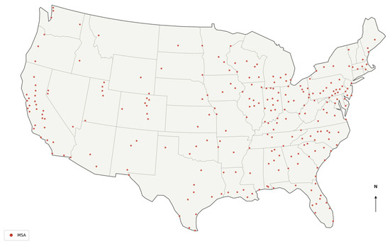
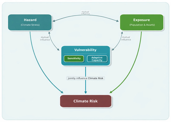
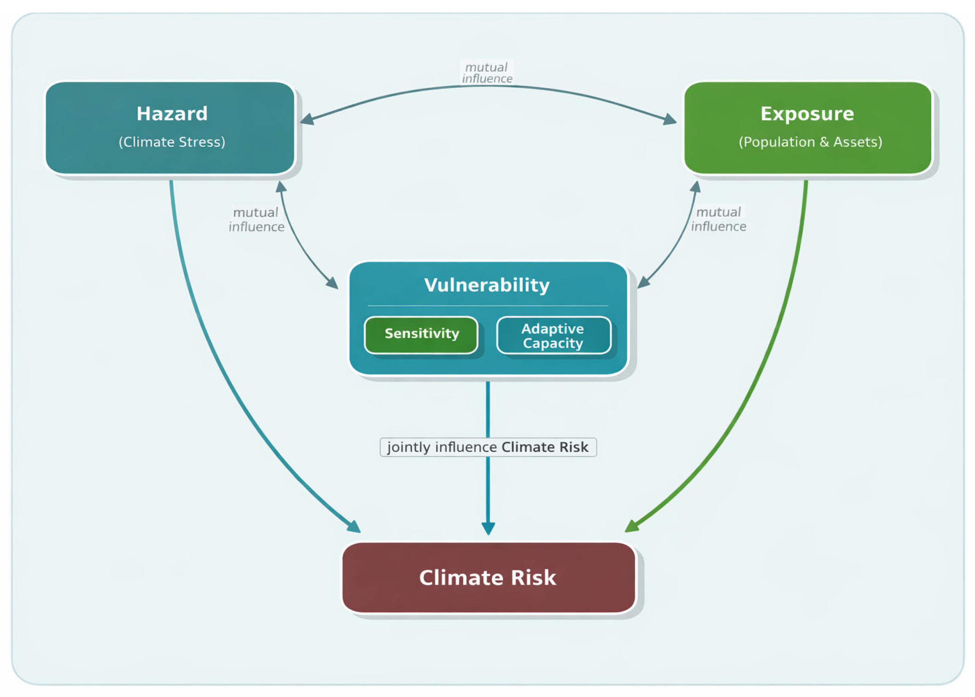
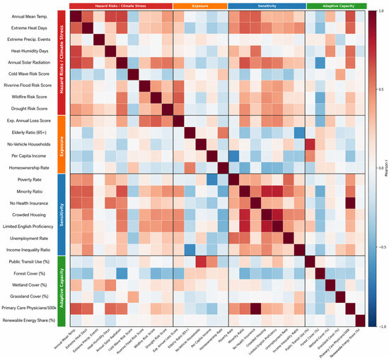
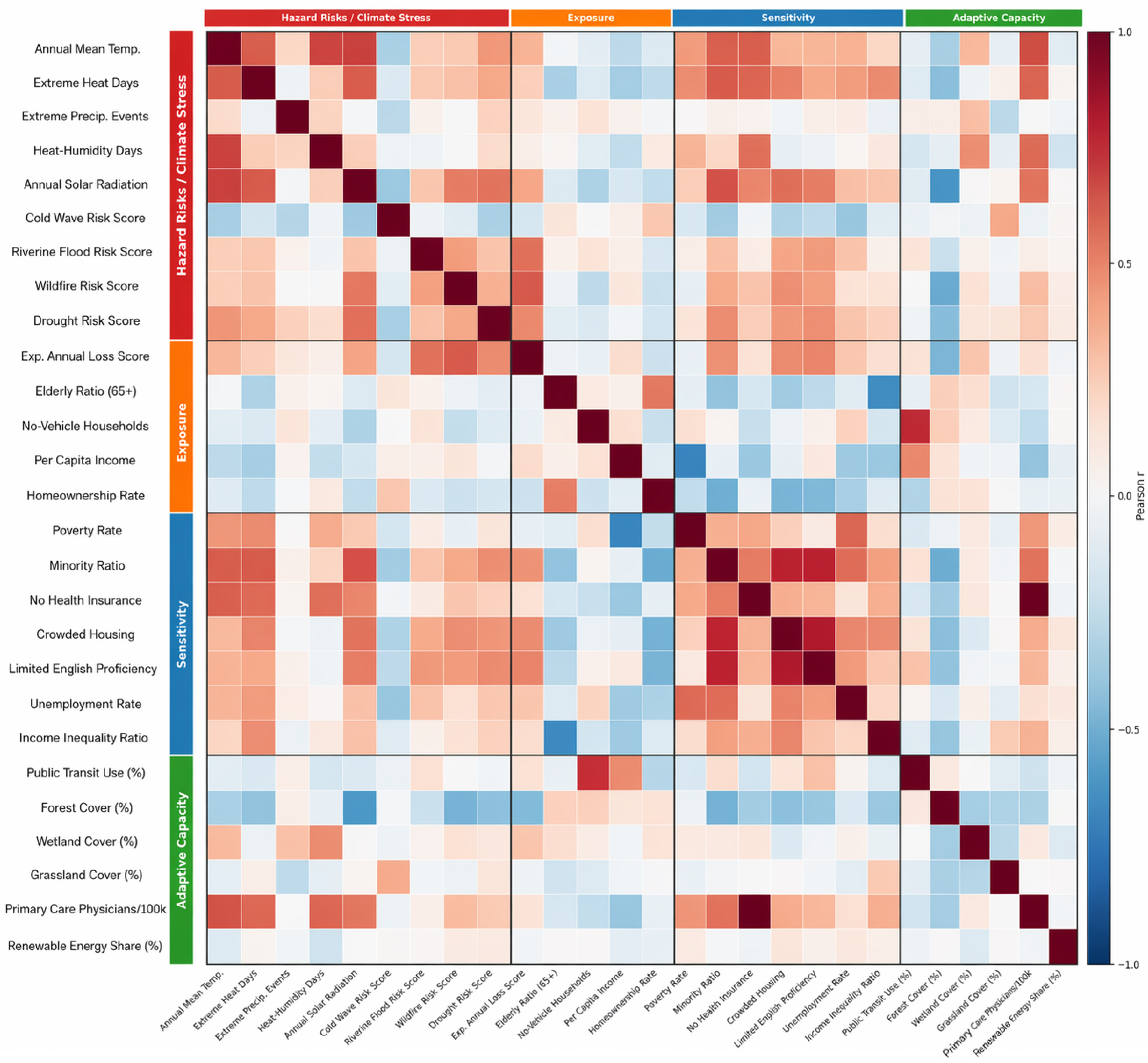
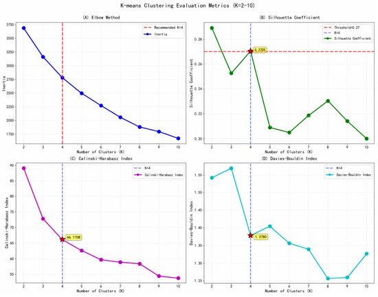
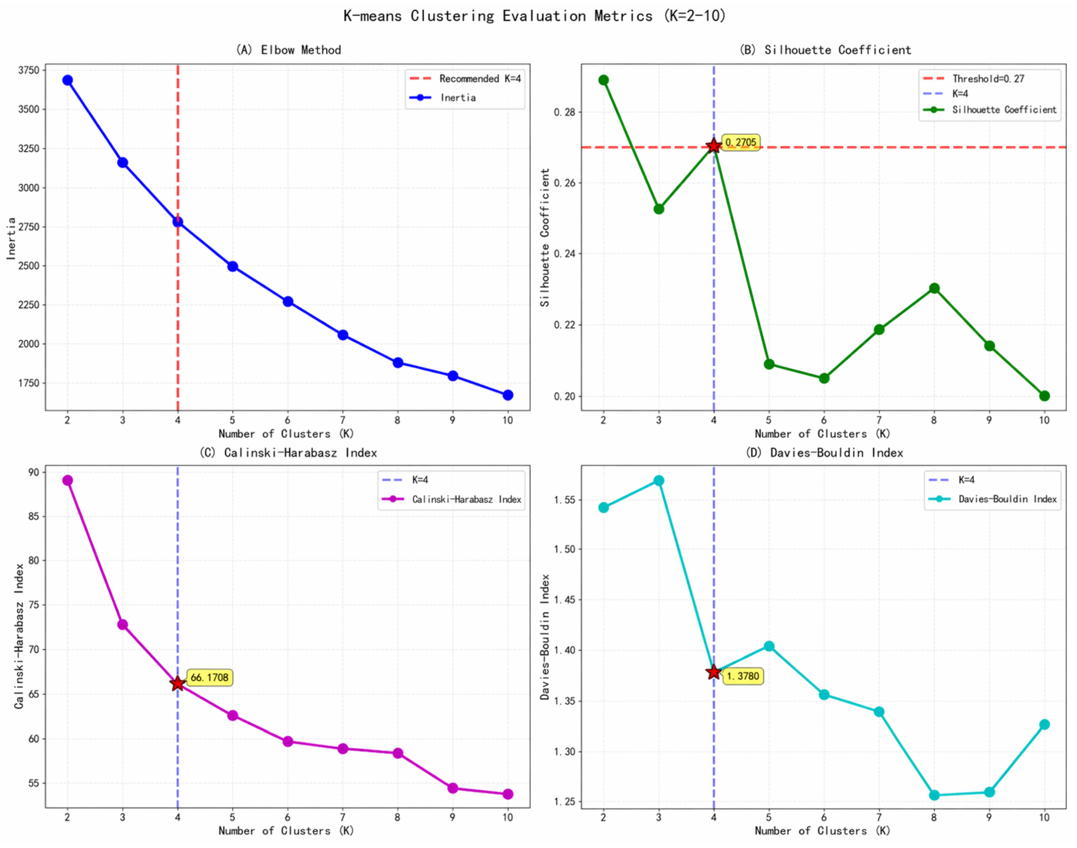
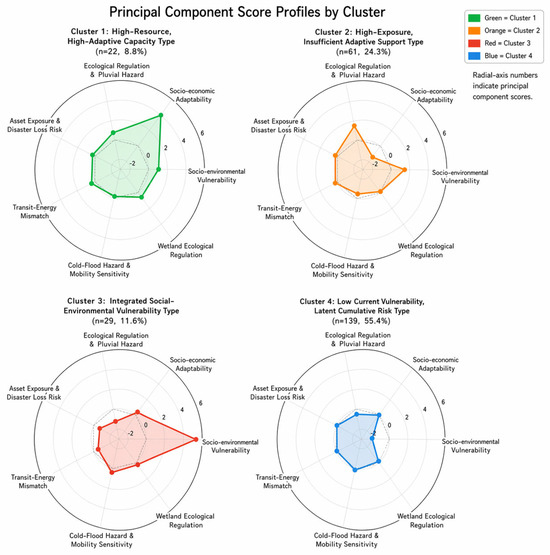
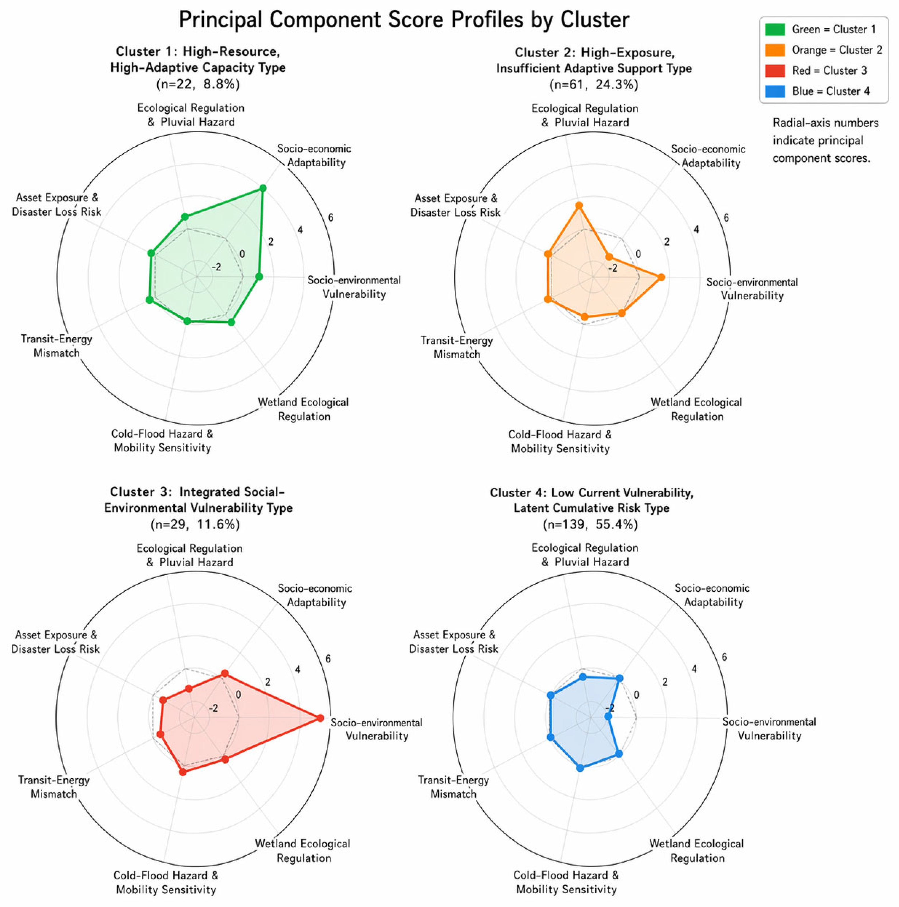
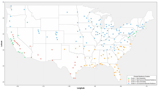
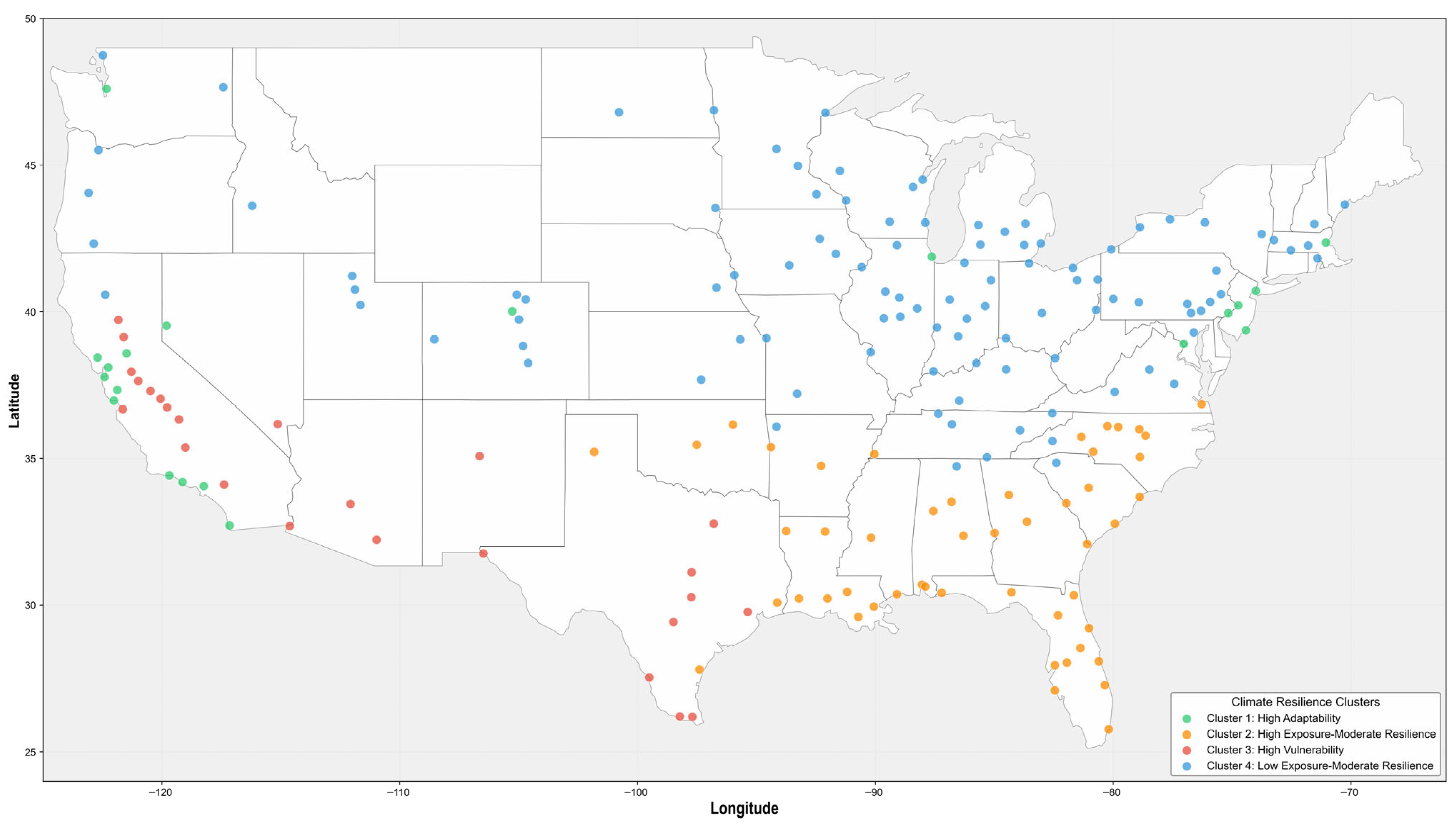

Disclaimer/Publisher’s Note: The statements, opinions and data contained in all publications are solely those of the individual author(s) and contributor(s) and not of MDPI and/or the editor(s). MDPI and/or the editor(s) disclaim responsibility for any injury to people or property resulting from any ideas, methods, instructions or products referred to in the content. |
© 2026 by the authors. Licensee MDPI, Basel, Switzerland. This article is an open access article distributed under the terms and conditions of the Creative Commons Attribution (CC BY) license.