Spatial and Vertical Distribution of Suspended Sediment Concentration in Haizhou Bay Based on Remote Sensing: Implications for Sustainable Coastal Management

Abstract

Suspended sediment concentration (SSC) strongly influences estuarine erosion–deposition processes, navigation safety, and coastal engineering stability. However, conventional remote sensing techniques are limited to surface SSC and cannot characterize vertical sediment structures. In this study, Landsat 8 OLI imagery was combined with in situ SSC profiles from six stations in the Guan River Estuary–Haizhou Bay system to retrieve full-depth sediment distributions. A band-combination inversion model using (B3 + B2)/B1 achieved the highest accuracy (R² = 0.679), and an improved vertical distribution model was developed by incorporating turbulent shear (G) into the Rouse framework. Results indicate that surface SSC ranged from 0.15 to 0.86 kg/m³, while middle- and bottom-layer SSC reached up to 1.20 kg/m³ and 1.77 kg/m³, respectively, exhibiting a consistent east–high and west–low spatial pattern. Settling velocity (SSV) varied from 3 × 10⁻⁶ to 1.49 × 10⁻² m/s and showed a positive correlation with SSC at low concentrations and a negative correlation at high concentrations due to flocculation effects. This integrated framework provides a rapid, low-cost method for full-water-column sediment assessment in estuaries and coastal zones, supporting engineering design, navigation maintenance, and sediment management. A better understanding of sediment transport processes in Haizhou Bay is important for maintaining shoreline stability and ecological balance in this semi-enclosed coastal system. The findings of this study provide a scientific basis for sediment management and environmental regulation, which can contribute to the long-term sustainable development of coastal environments in the Yellow Sea region.

1. Introduction

Sediment transport in estuarine and coastal environments is influenced by multiple hydrodynamic factors. Among them, suspended sediment concentration (SSC) and sediment settling velocity (SSV) are two key variables controlling sediment dynamics. Variations in these parameters influence erosion and deposition patterns, navigation channel maintenance, and the stability of coastal engineering structures. Conventional field sampling methods can provide highly accurate measurements; however, their spatial and temporal coverage is often limited, particularly in highly dynamic estuarine systems. In recent decades, satellite remote sensing has emerged as an efficient approach for monitoring suspended sediments over large spatial scales because it enables rapid and repeated observations. Nevertheless, most satellite-based approaches primarily retrieve surface SSC and cannot independently characterize the vertical structure of suspended sediments within the water column.

The application of remote sensing to estimate SSC can be traced back to the 1970s. Early work by Williamson and Grabau [1] demonstrated that satellite-derived radiance exhibits a measurable relationship with suspended sediment concentration in Chesapeake Bay. Subsequent studies by Curran and Novo [2], based on investigations in European and South American coastal waters, further developed semi-empirical relationships linking water reflectance in visible and near-infrared bands to sediment concentration. Since the beginning of the 21st century, advances in sensor technology and data availability have enabled multisensory approaches and long-term monitoring of suspended sediments. For example, Nechad et al. [3] proposed a generic algorithm for retrieving total suspended matter in turbid European coastal waters, improving the consistency of SSC estimation across different satellite sensors. Similar remote sensing techniques have been widely applied in major estuarine and coastal systems worldwide, including the Yangtze River Estuary, Pearl River Estuary, Amazon continental shelf, and the Ganges–Brahmaputra estuarine system [4,5,6,7].

Despite these advances, most remote sensing studies focus primarily on surface SSC and implicitly assume vertically uniform sediment conditions. Such assumptions are rarely valid in estuarine environments, where hydrodynamic processes such as tidal mixing, turbulent shear, density-driven circulation, and sediment flocculation frequently generate strong vertical gradients in sediment concentration. Neglecting these vertical variations may reduce the reliability of remote sensing-based sediment assessments, particularly in practical applications such as channel siltation prediction, coastal engineering design, and sediment management. Furthermore, classical theoretical approaches describing vertical sediment distribution, such as the Rouse equation, were originally derived under steady and uniform flow conditions in rivers. These assumptions are often difficult to satisfy in nearshore and estuarine environments where hydrodynamic forcing is more complex and highly variable.

To address these limitations, this study combines satellite-based SSC inversion with sediment diffusion theory to estimate the vertical distribution of suspended sediments. The Guan River Estuary and the adjacent Haizhou Bay are selected as the study area, where Landsat 8 imagery is integrated with field measurements of SSC profiles and current velocity. By introducing the turbulence shear parameter (G) into the classical Rouse framework, an improved model is developed to better represent sediment dynamics under non-uniform flow conditions. The main objectives of this study are to: (1) establish a reliable surface SSC inversion model using multispectral band combinations; (2) develop an improved vertical distribution model that incorporates turbulence effects; (3) analyze the spatial and temporal patterns of SSC and SSV in the study area; and (4) discuss the implications of these findings for sediment regulation and sustainable management of estuarine and coastal environments.

Understanding the spatial and vertical variability of suspended sediments is essential for maintaining the ecological stability and morphological balance of coastal systems. Improved knowledge of sediment transport processes can support more sustainable coastal management strategies, particularly in regions where sediment dynamics strongly influence shoreline evolution, navigation channels, and marine ecosystems. Such insights contribute to the broader goal of promoting environmentally sustainable development and long-term resilience of estuarine and coastal zones.

2. Materials and Methods

2.1. Study Area

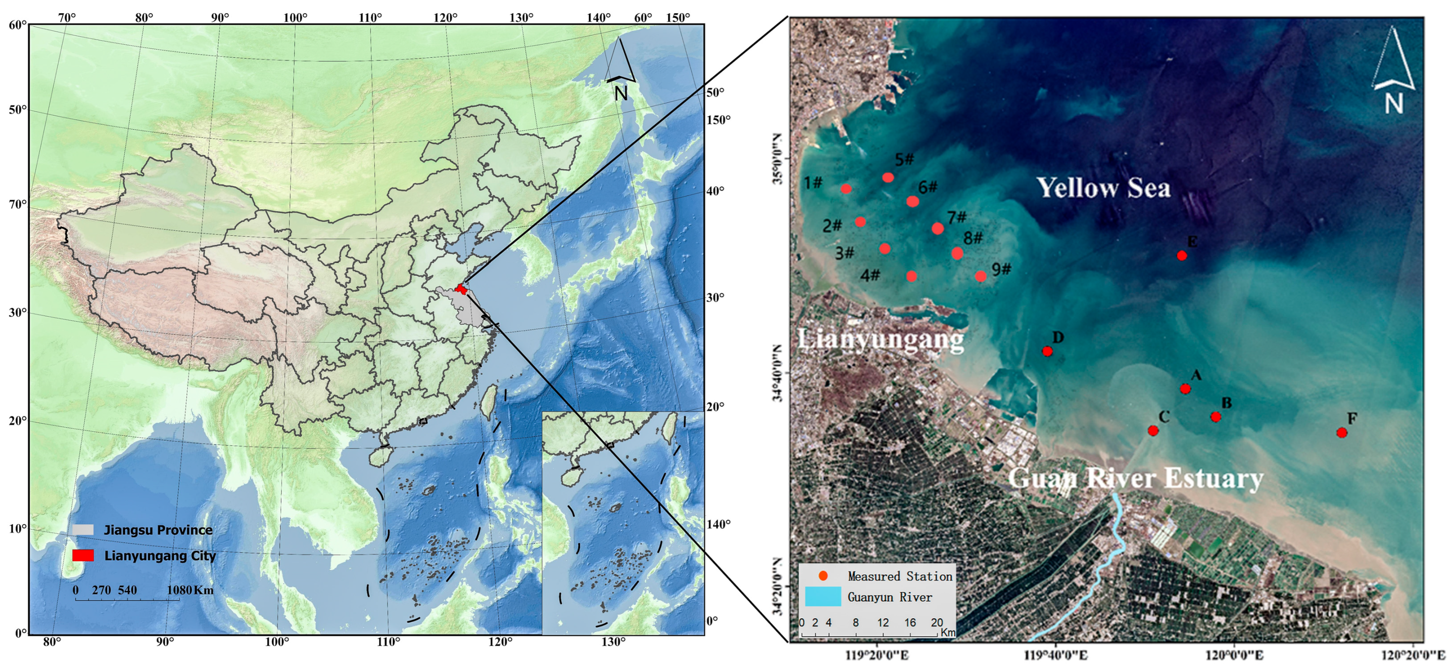
The Guan River is an important natural river system located in northern Jiangsu Province, and its main channel is not regulated by sluice gates (Figure 1). The river is approximately 74.5 km long and drains a watershed of about 6400 km². It discharges into Haizhou Bay, a semi-enclosed coastal basin situated in the western part of the Yellow Sea. The hydrodynamic conditions in the Guan River Estuary are primarily influenced by irregular semidiurnal tides, which are associated with relatively large tidal ranges and strong tidal currents [8,9].

Figure 1. Research area.

Within the estuarine channel, deformation of the tidal wave under boundary constraints produces a mixed standing-wave pattern, characterized by shorter flood durations and relatively longer ebb phases. In the adjacent coastal zone, the nearshore circulation generally forms a counterclockwise rotational pattern, whereas the flow at the estuary mouth and over nearby shoals is mainly reciprocating in nature. Wave observations from Kaishan Island, located about 9 km offshore, indicate that the dominant wave direction is from the northeast (NE), while stronger wave events typically originate from the east-northeast (ENE). The maximum recorded wave height in this area reaches approximately 3.0 m.

The seabed sediments within the estuary are mainly composed of silt and fine sand, forming a typical silty–muddy coastal environment [10]. Extensive shoals develop outside the estuary, where wave activity frequently resuspends bottom sediments and contributes to the redistribution of suspended materials in the nearshore waters.

Data processing and figure generation were performed using ArcGIS Pro 3.5.2 (ESRI, Redlands, CA, USA), ArcMap 10.8.2 (ESRI, Redlands, CA, USA), Surfer 26 (Golden Software, LLC, Golden, CO, USA), and Origin 2023b (OriginLab Corporation, Northampton, MA, USA).

2.2. Data Source

2.2.1. Remote Sensing Data

Landsat 8 OLI–TIRS imagery was obtained from the Geospatial Data Cloud and USGS Earth. Explorer platforms. The selected image (Identifier: LC81180382016138LGN00) was acquired at 02:36 UTC on 29 April 2016, with cloud coverage less than 10%, satisfying the requirements for quantitative water-quality inversion. The image includes 11 spectral bands [Table 1], with spatial resolutions of 30 m for OLI bands (B1–B7, B9), 15 m for the panchromatic band (B8), and 100 m for TIRS bands (B10–B11). The central meridian is 114.989° E, and the coordinate system is WGS 84 with UTM Zone 50N projection.

Table 1. Main characteristics and applications of Landsat 8 spectral bands.

Band Name	Resolution (m)	Wavelength (μm)	Application
Band 1 Coastal	30	0.43~0.45	Coastal zone observation
Band 2 Blue	30	0.45~0.51	Water penetrates to distinguish soil and vegetation
Band 3 Green	30	0.53~0.59	Distinguish vegetation
Band 4 Red	30	0.64~0.67	It is located in the chlorophyll absorption zone and is used to observe roads and exposed soil. Types of vegetation, etc.
Band 5 NIR	30	0.85~0.88	Estimate biomass and distinguish moist soil
Band 6 SWIR 1	30	1.57~1.65	It is used to distinguish roads, exposed soil and water, and has a good ability to distinguish the atmosphere and clouds and fog
Band 7 SWIR 2	30	2.11~2.99	Distinguish minerals and rocks, and identify moist soil
Band 8 Pan	15	0.50~0.68	A 15 m resolution black-and-white image for enhancing resolution
Band 9 Cirrus	30	1.36~1.38	It features strong water vapor absorption and can be used for cloud detection
Band 10 TIRS 1	100	10.60~11.19	The target of induced thermal radiation
Band 11 TIRS 2	100	11.50~12.51	The target of induced thermal radiation

Only the OLI coastal (B1), blue (B2), green (B3), and red (B4) bands were used for SSC inversion, consistent with previous studies demonstrating their sensitivity to suspended sediments in turbid coastal waters [3]. Image selection prioritized minimal cloud cover, low atmospheric aerosol loading, and temporal proximity to in situ measurements to reduce spatiotemporal mismatch errors. In situ observations were temporally matched to the satellite overpass with a maximum allowable time difference of ±1 h. Spatially, reflectance values were extracted from the nearest cloud-free pixel within a 3 × 3-pixel window centered on each station to minimize geolocation and sub-pixel variability effects.

2.2.2. In Situ Measurements

To satisfy the requirements of both remote sensing inversion modeling and vertical sediment structure analysis, two types of sampling stations were designed: (1) six fixed long-term observation stations (Stations A–F), The sampling stations were selected to represent key hydrodynamic and sedimentary conditions across the estuary and coastal zone. Site placement considered bathymetry, tidal currents, sediment transport pathways, and field accessibility to ensure coverage of river-influenced, tidally mixed, and offshore areas. where field measurements were conducted during spring tide (25–26 April 2016) and neap tide (29–30 April 2016). Each survey lasted approximately 25 h, with hourly water sampling at multiple depths according to local water depth. Suspended sediment concentration (SSC) was determined using the filter membrane gravimetric method following standardized laboratory procedures. Velocity profiles were measured using an acoustic Doppler current profiler (ADCP) to calculate turbulent shear and associated hydrodynamic parameters. All measurements followed national and international standards for coastal and estuarine surveys. The method is as shown in Table 2; and (2) nine remote sensing matching sites (Site1#–Site9#), used for spatial collocation with satellite pixels to improve the spatial representativeness of the inversion model. The Site locations were not independently established stations but supplementary sampling points within the spatial vicinity of the fixed stations, intended to reduce the scale mismatch between satellite pixels and point-based field measurements.

Table 2. The time and method for obtaining sediment data.

Study Area	Seawater Bay
Number of Stations	6 fixed observation stations
Tidal Phase	Spring Tide	Neap Tide
Observation Date	25 April 2016–26 April 2016	29 April 2016–30 April 2016
Observation Period	10:00, 25 April 2016–10:00, 26 April 2016	07:00, 29 April 2016–07:00, 30 April 2016
Duration	25 h
Sampling Frequency	Hourly water sampling
Sampling Method	Methods varied according to water depth
Parameter Measured	Suspended Sediment Concentration (SSC)
Analytical Method	Filter membrane gravimetric method

During the experiment, the operation was strictly in accordance with the relevant specifications. Firstly, the filter membrane was used to filter the water sample. Secondly, the vacuum filter was used to filter it. The filtered sample was placed in an aluminum box and dried in an oven. After cooling, it was weighed. Finally, the suspended sediment concentration of the sample was calculated using the equation.

2.2.3. Preprocessing of Remote Sensing Data

Remote sensing images require several preprocessing procedures before quantitative analysis can be performed. In this study, the preprocessing workflow mainly included radiometric calibration, atmospheric correction, and image clipping.

• Radiation calibration.

The digital numbers recorded by satellite sensors are affected by instrumental noise and other systematic factors. Therefore, radiometric calibration is necessary to convert the original digital values into physically meaningful radiance values. In this study, Landsat 8 imagery was processed using ENVI 5.2 (Environment for Visualizing Images). The radiometric calibration tool in the Toolbox was applied to convert the raw image data into calibrated radiance values, which improves the reliability of subsequent spectral analysis.

2.

Atmospheric correction.

Satellite observations are influenced by atmospheric scattering and absorption, which may distort the spectral signal received by the sensor. Consequently, atmospheric correction is required to obtain surface reflectance that more accurately represents the optical properties of water bodies. This step reduces the influence of atmospheric components such as aerosols and water vapor, thereby improving the accuracy of suspended sediment retrieval. After atmospheric correction, the reflectance values of the water surface become more representative of the actual conditions, providing a more reliable basis for subsequent inversion analysis.

3.

Image cropping.

After radiometric and atmospheric corrections, the Landsat image was clipped to the region of interest covering the Guan River Estuary and the adjacent Haizhou Bay. During this step, areas affected by cloud cover were excluded to avoid interference with the spectral analysis. In addition, excessively deep offshore regions were not included in the clipped image, because extremely low reflectance values in deep water may produce negative band values that can influence subsequent model calculations. The final processed image therefore focuses on the nearshore zone where suspended sediment dynamics are most significant.

2.3. Method

2.3.1. Spectral Extraction from Remote Sensing Images

The optical characteristics of water bodies vary with changes in the composition and concentration of suspended materials. Variations in suspended sediment content alter the spectral reflectance of water, which can be detected by satellite sensors. Remote sensing inversion of suspended sediment concentration (SSC) is therefore based on establishing relationships between the spectral signals recorded by sensors and the corresponding sediment concentration in the water column [11]. To estimate SSC, spectral information from satellite imagery must first be extracted for the corresponding sampling locations. In practice, this involves obtaining reflectance values from individual spectral bands and relating them to the measured SSC data. The reflectance values derived from remote sensing images represent the integrated response of the sensor within specific wavelength ranges, which correspond to the spectral sensitivity of each band [12]. Based on previous studies on suspended sediment retrieval in turbid coastal waters, Landsat 8 OLI imagery was selected in this study. Four spectral bands were used for SSC inversion, including the coastal band (B1), blue band (B2), green band (B3), and red band (B4). Their wavelength ranges are 0.43–0.45 μm (B1), 0.45–0.51 μm (B2), 0.53–0.59 μm (B3), and 0.64–0.67 μm (B4), respectively. These bands are widely considered sensitive to variations in suspended sediment in coastal environments. Using ENVI 5.2, the reflectance values of these four bands were extracted for each sampling station in the study area. The corresponding equivalent reflectance values are listed in Table 3.

Table 3. Landsat 8 OLI B1, B2, B3, B4 spectral reflectance equivalent value of each measured point.

Site	B1	B2	B3	B4
1#	0.059702	0.051660	0.061631	0.028897
2#	0.062753	0.053403	0.061066	0.025936
3#	0.062905	0.058154	0.071310	0.035601
4#	0.068241	0.063388	0.077164	0.043033
5#	0.052764	0.044949	0.047883	0.013292
6#	0.069171	0.064092	0.081904	0.052539
7#	0.066305	0.058325	0.069595	0.035689
8#	0.062582	0.056905	0.065668	0.030104
9#	0.052787	0.044319	0.045123	0.013339

To further improve the reliability of the inversion model, different band ratios were calculated based on the extracted reflectance values. Band ratios can effectively reduce the influence of illumination conditions and atmospheric residual errors, thereby enhancing the sensitivity of the spectral signal to suspended sediments. The calculated ratios for each station are presented in Table 4.

Table 4. The ratio of the equivalent reflectance values of each band of Landsat 8 OLI spectrum at each measured point.

Site	B4/B3	B4/B2	B4/B1	B3/B2	B3/B1	B2/B1
1#	0.468875	0.559372	0.484031	1.193011	1.032324	0.865310
2#	0.424718	0.485668	0.413299	1.143506	0.973112	0.850990
3#	0.499235	0.612173	0.565941	1.226222	1.133615	0.924478
4#	0.557674	0.678879	0.630597	1.217341	1.130763	0.928880
5#	0.277597	0.295719	0.251921	1.065283	0.907508	0.851894
6#	0.641478	0.819746	0.759556	1.277902	1.184072	0.926575
7#	0.512806	0.611891	0.538247	1.193220	1.049611	0.879646
8#	0.458423	0.529017	0.481030	1.153992	1.049315	0.909291
9#	0.295621	0.300987	0.252700	1.018150	0.854813	0.839574

In addition to simple band ratios, several multi-band combination indices were also constructed using the four spectral bands. These combinations were used to test different empirical relationships between spectral reflectance and SSC in order to identify the most suitable inversion model for the study area. The calculated band-combination indices are shown in Table 5.

Table 5. Combination values of equivalent reflectance values of each band of Landsat 8 OLI spectrum of each measured point.

Site	B4/(B3 + B2)	B4/(B3 + B1)	B3/(B2 + B1)	(B4 + B3)/B2	(B3 + B2)/B1
1#	0.255071	0.238166	0.553433	1.752383	1.897634
2#	0.226577	0.209465	0.525725	1.629175	1.824102
3#	0.274983	0.265250	0.589051	1.838394	2.058094
4#	0.306168	0.295949	0.586228	1.896220	2.059643
5#	0.143186	0.132068	0.490043	1.361002	1.759403
6#	0.359869	0.347771	0.614600	2.097648	2.110647
7#	0.278992	0.262609	0.558409	1.805110	1.929258
8#	0.245598	0.234727	0.549584	1.683009	1.958606
9#	0.149140	0.136240	0.464680	1.319137	1.694387

2.3.2. Landsat-8-Based SSC Inversion Model

To retrieve suspended sediment concentration (SSC) from Landsat 8 imagery, empirical relationships between spectral reflectance and measured SSC were established using regression analysis. The performance of the inversion models was evaluated using the coefficient of determination (R²), which reflects the degree of agreement between observed and predicted values.

The coefficient of determination is calculated as:

$${\mathrm{R}}^2={\displaystyle \frac{{\sum }_{\mathrm{i}=1}^{\mathrm{n}}{({\mathrm{y}}_{\mathrm{i}}- \stackrel{-}{\mathrm{y}})}^2-{\sum }_{\mathrm{i}=1}^{\mathrm{n}}{\left({\mathrm{y}}_{\mathrm{i}}-{\mathrm{f}}_{\mathrm{i}}\right)}^2}{{\sum }_{\mathrm{i}=1}^{\mathrm{n}}{({\mathrm{y}}_{\mathrm{i}}- \stackrel{-}{\mathrm{y}})}^2}}$$

(1)

where ${\mathrm{y}}_{\mathrm{i}}$ represents the measured SSC; $\stackrel{-}{\mathrm{y}}$ is the mean of the measured values; ${\mathrm{f}}_{\mathrm{i}}$ is the predicted value obtained from the regression model; and $\mathrm{n}$ is the number of samples.

(1)

Single-band SSC inversion model.

In the single-band approach, the reflectance values of Landsat 8 bands B1, B2, B3, and B4 were individually used as independent variables, while the measured SSC values served as the dependent variable. Regression relationships were established for each spectral band to evaluate their capability in estimating SSC.

The regression results for the four bands are summarized in Table 6, Table 7, Table 8 and Table 9.

Table 6. Inversion model construction of the relationship between B1 band and suspended sediment concentration and its correlation coefficients.

Band	Model	Relation	${\mathbf{R}}^2$
B1	Linear function model of one order	$\mathrm{y}=0.22485\mathrm{x}-0.07854$	0.3303
	Quadratic polynomial function model	$\mathrm{y}=-0.06737{\mathrm{x}}^2+0.30636\mathrm{x}-0.103$	0.3304
	Exponential function model	$\mathrm{y}=0.0042{\mathrm{e}}^{4.2017\mathrm{x}}$	0.3292
	Logarithmic function model	$\mathrm{y}=0.13525\ln \left(\mathrm{x}\right) +0.1261$	0.3308

Note: y denotes the suspended sediment concentration (SSC). B1–B4 represent the first four spectral bands of Landsat 8 imagery, and x indicates the corresponding reflectance values extracted using ENVI 5.2.

Table 7. Inversion model construction of the relationship between B2 band and suspended sediment concentration and its correlation coefficients.

Band	Model	Relation	${\mathbf{R}}^2$
B2	Linear function model of one order	$\mathrm{y}=0.22387\mathrm{x}-0.06251$	0.4653
	Quadratic polynomial function model	$\mathrm{y}=0.51902{\mathrm{x}}^2-0.33597\mathrm{x}+0.08606$	0.4746
	Exponential function model	$\mathrm{y}=0.0058{\mathrm{e}}^{4.1364\mathrm{x}}$	0.4533
	Logarithmic function model	$\mathrm{y}=0.11841\ln \left(\mathrm{x}\right)+0.13233$	0.4577

Note: y denotes the suspended sediment concentration (SSC). B1–B4 represent the first four spectral bands of Landsat 8 imagery, and x indicates the corresponding reflectance values extracted using ENVI 5.2.

Table 8. Inversion model construction of the relationship between B3 band and suspended sediment concentration and its correlation coefficients.

Band	Model	Relation	${\mathbf{R}}^2$
B3	Linear function model of one order	$\mathrm{y}=0.13719\mathrm{x}-0.02795$	0.5195
	Quadratic polynomial function model	$\mathrm{y}=0.04779{\mathrm{x}}^2+0.07724\mathrm{x}-0.0098$	0.5203
	Exponential function model	$\mathrm{y}=0.0108{\mathrm{e}}^{2.5561\mathrm{x}}$	0.5147
	Logarithmic function model	$\mathrm{y}=0.08317\ln \left(\mathrm{x}\right) +0.09846$	0.5127

Note: y denotes the suspended sediment concentration (SSC). B1–B4 represent the first four spectral bands of Landsat 8 imagery, and x indicates the corresponding reflectance values extracted using ENVI 5.2.

Table 9. Inversion model construction of the relationship between B4 band and suspended sediment concentration and its correlation coefficients.

Band	Model	Relation	${\mathbf{R}}^2$
B4	Linear function model of one order	$\mathrm{y}=0.12767\mathrm{x}+0.02117$	0.487
	Quadratic polynomial function model	$\mathrm{y}=-0.10635{\mathrm{x}}^2+0.19427\mathrm{x}+0.01229$	0.4933
	Exponential function model	$\mathrm{y}=0.0272{\mathrm{e}}^{2.3403\mathrm{x}}$	0.4672
	Logarithmic function model	$\mathrm{y}=0.03405\ln \left(\mathrm{x}\right)+0.1037$	0.4802

Note: y denotes the suspended sediment concentration (SSC). B1–B4 represent the first four spectral bands of Landsat 8 imagery, and x indicates the corresponding reflectance values extracted using ENVI 5.2.

Among the tested models, the linear relationship based on the B3 band produced the highest correlation coefficient, with an R² value of 0.5195. In general, bands B2 and B3 showed stronger correlations with SSC than bands B1 and B4.

However, the overall performance of the single-band models was relatively limited, indicating that SSC retrieval based on a single spectral band may not adequately capture the optical variability of turbid coastal waters. Consequently, the accuracy of SSC estimation in the nearshore waters of Lianyungang remains insufficient when relying solely on single-band relationships.

In coastal waters, the spectral signal detected by satellite sensors is influenced not only by suspended sediments but also by other optically active substances, such as chlorophyll and colored dissolved organic matter. These factors can affect the spectral characteristics of water and introduce uncertainty into SSC retrieval models. To reduce such interference and improve inversion accuracy, it is therefore necessary to incorporate information from multiple spectral bands.

(2)

Two-Band-ratio SSC inversion model

To further enhance the performance of the inversion model, band-ratio methods were applied. In this approach, ratios between two spectral bands were used as independent variables to establish regression relationships with measured SSC. Band ratios are commonly used in water quality retrieval because they can reduce the influence of illumination conditions and atmospheric effects, thereby improving the sensitivity of spectral signals to suspended sediments.

As shown in the table above Table 10, Table 11, Table 12, Table 13, Table 14 and Table 15, the two-band ratio models based on Bands B1–B4 exhibit overall higher correlations with the measured suspended sediment concentration (SSC) than the single-band models. Among them, the B3/B1 index model achieves the highest correlation coefficient (0.6602). Multiple models based on the B3/B1 ratio and all models based on the B2/B1 ratio show correlation coefficients exceeding 0.6, whereas the B4/B2 ratio exhibits relatively poor fitting performance. Overall, the two-band ratio approach provides better inversion performance. To further improve model accuracy, multi-band combination fitting is required to identify the optimal remote sensing inversion model for SSC in the nearshore waters of Haizhou Bay.

Table 10. Inversion model construction of the relationship between B4/B3 band and suspended sediment concentration and its correlation coefficients.

Band	Model	Relation	${\mathbf{R}}^2$
B4/B3	Linear function model of one order	$\mathrm{y}=0.1369\mathrm{x}-0.0022$	0.4638
	Quadratic polynomial function model	$\mathrm{y}=0.0118{\mathrm{x}}^2+0.1264\mathrm{x}-0.0005$	0.4639
	Exponential function model	$\mathrm{y}=0.0176{\mathrm{e}}^{2.526\mathrm{x}}$	0.451
	Logarithmic function model	$\mathrm{y}=0.0566\ln \left(\mathrm{x}\right)+0.1065$	0.4496

Note: y denotes the suspended sediment concentration (SSC). B1–B4 represent the first four spectral bands of Landsat 8 imagery, and x indicates the corresponding reflectance values extracted using ENVI 5.2.

Table 11. Inversion model construction of the relationship between B4/B2 band and suspended sediment concentration and its correlation coefficients.

Band	Model	Relation	${\mathbf{R}}^2$
B4/B2	Linear function model of one order	$\mathrm{y}=0.0967\mathrm{x}+0.0081$	0.4875
	Quadratic polynomial function model	$\mathrm{y}=-0.0361{\mathrm{x}}^2+0.1351\mathrm{x}-0.0012$	0.4897
	Exponential function model	$\mathrm{y}=0.0212{\mathrm{e}}^{1.7915\mathrm{x}}$	0.4771
	Logarithmic function model	$\mathrm{y}=0.0467\ln \left(\mathrm{x}\right)+0.0914$	0.4786

Note: y denotes the suspended sediment concentration (SSC). B1–B4 represent the first four spectral bands of Landsat 8 imagery, and x indicates the corresponding reflectance values extracted using ENVI 5.2.

Table 12. Inversion model construction of the relationship between B4/B1 band and suspended sediment concentration and its correlation coefficients.

Band	Model	Relation	${\mathbf{R}}^2$
B4/B1	Linear function model of one order	$\mathrm{y}=0.1024\mathrm{x}+0.0109$	0.5255
	Quadratic polynomial function model	$\mathrm{y}=-0.0441{\mathrm{x}}^2+0.1449\mathrm{x}+0.0017$	0.5285
	Exponential function model	$\mathrm{y}=0.0224{\mathrm{e}}^{1.8868\mathrm{x}}$	0.5091
	Logarithmic function model	$\mathrm{y}=0.0442\ln \left(\mathrm{x}\right)+0.0951$	0.5148

Note: y denotes the suspended sediment concentration (SSC). B1–B4 represent the first four spectral bands of Landsat 8 imagery, and x indicates the corresponding reflectance values extracted using ENVI 5.2.

Table 13. Inversion model construction of the relationship between B3/B2 band and suspended sediment concentration and its correlation coefficients.

Band	Model	Relation	${\mathbf{R}}^2$
B3/B2	Linear function model of one order	$\mathrm{y}=0.2169\mathrm{x}-0.1922$	0.5687
	Quadratic polynomial function model	$\mathrm{y}=0.0384{\mathrm{x}}^2+0.1292\mathrm{x}-0.1423$	0.5689
	Exponential function model	$\mathrm{y}=0.0004{\mathrm{e}}^{4.1644\mathrm{x}}$	0.5981
	Logarithmic function model	$\mathrm{y}=0.2467\ln \left(\mathrm{x}\right) +0.0235$	0.5675

Note: y denotes the suspended sediment concentration (SSC). B1–B4 represent the first four spectral bands of Landsat 8 imagery, and x indicates the corresponding reflectance values extracted using ENVI 5.2.

Table 14. Inversion model construction of the relationship between B3/B1 band and suspended sediment concentration and its correlation coefficients.

Band	Model	Relation	${\mathbf{R}}^2$
B3/B1	Linear function model of one order	$\mathrm{y}=0.1753\mathrm{x}-0.1208$	0.6604
	Quadratic polynomial function model	$\mathrm{y}=0.01764{\mathrm{x}}^{2 }+0.13935\mathrm{x}-0.10263$	0.6604
	Exponential function model	$\mathrm{y}=0.0019{\mathrm{e}}^{3.2956\mathrm{x}}$	0.6662
	Logarithmic function model	$\mathrm{y}=0.17691\ln \left(\mathrm{x}\right)+0.0555$	0.6581

Note: y denotes the suspended sediment concentration (SSC). B1–B4 represent the first four spectral bands of Landsat 8 imagery, and x indicates the corresponding reflectance values extracted using ENVI 5.2.

Table 15. Inversion model construction of the relationship between B2/B1 band and suspended sediment concentration and its correlation coefficients.

Band	Model	Relation	${\mathbf{R}}^2$
B2/B1	Linear function model of one order	$\mathrm{y}=0.5238\mathrm{x}-0.4036$	0.6594
	Quadratic polynomial function model	$\mathrm{y}=0.8394{\mathrm{x}}^2-0.9652\mathrm{x}+0.2558$	0.66
	Exponential function model	$\mathrm{y}=1 \times {10}^{-5} {\mathrm{e}}^{9.5979\mathrm{x}}$	0.6317
	Logarithmic function model	$\mathrm{y}=0.4642\ln \left(\mathrm{x}\right)+0.117$	0.659

Note: y denotes the suspended sediment concentration (SSC). B1–B4 represent the first four spectral bands of Landsat 8 imagery, and x indicates the corresponding reflectance values extracted using ENVI 5.2.

(3)

Multi-band SSC inversion model

After combining Bands B1, B2, B3, and B4 in various multi-band configurations, correlation-based inversion models were developed between the spectral indices and the measured suspended sediment concentration (SSC) in the nearshore waters, and corresponding regression equations were established Table 16, Table 17, Table 18, Table 19, Table 20, Table 21, Table 22, Table 23 and Table 24. The fitting results indicate that combinations among Bands B1, B2, and B3 yield slightly higher correlation coefficients than other functional models. Consistent with previous findings, models involving Band B4 show relatively poor correlations with SSC. Therefore, Band B4 was excluded from the regression models used for SSC inversion in the nearshore waters of Haizhou Bay.

Table 16. Inversion model construction of the relationship between B4/(B3 + B2) band and suspended sediment concentration and its correlation coefficients.

Band	Model	Relation	${\mathbf{R}}^2$
B4/(B3 + B2)	Linear function model of one order	$\mathrm{y}=0.2319\mathrm{x}+0.003$	0.4771
	Quadratic polynomial function model	$\mathrm{y}=-0.0839{\mathrm{x}}^2+0.2724\mathrm{x}-0.0015$	0.4774
	Exponential function model	$\mathrm{y}=0.0193{\mathrm{e}}^{4.2891\mathrm{x}}$	0.4659
	Logarithmic function model	$\mathrm{y}=0.0516\ln \left(\mathrm{x}\right)+0.1345$	0.465

Note: y denotes the suspended sediment concentration (SSC). B1–B4 represent the first four spectral bands of Landsat 8 imagery, and x indicates the corresponding reflectance values extracted using ENVI 5.2.

Table 17. Inversion model construction of the relationship between B4/(B3 + B1) band and suspended sediment concentration and its correlation coefficients.

Band	Model	Relation	${\mathbf{R}}^2$
B4/(B3 + B1)	Linear function model of one order	$\mathrm{y}=0.2367\mathrm{x}+0.0048$	0.5007
	Quadratic polynomial function model	$\mathrm{y}=-0.0969{\mathrm{x}}^2+0.2813\mathrm{x}+0.0001$	0.5011
	Exponential function model	$\mathrm{y}=0.02{\mathrm{e}}^{4.3696\mathrm{x}}$	0.4868
	Logarithmic function model	$\mathrm{y}=0.0498\ln \left(\mathrm{x}\right) +0.1348$	0.4872

Note: y denotes the suspended sediment concentration (SSC). B1–B4 represent the first four spectral bands of Landsat 8 imagery, and x indicates the corresponding reflectance values extracted using ENVI 5.2.

Table 18. Inversion model construction of the relationship between B3/(B2 + B1) band and suspended sediment concentration and its correlation coefficients.

Band	Model	Relation	${\mathbf{R}}^2$
B3/(B2 + B1)	Linear function model of one order	$\mathrm{y}=0.3869\mathrm{x}-0.1513$	0.6332
	Quadratic polynomial function model	$\mathrm{y}=0.184{\mathrm{x}}^2+0.1888\mathrm{x}-0.0984$	0.6335
	Exponential function model	$\mathrm{y}={0.001\mathrm{e}}^{7.3308\mathrm{x}}$	0.6488
	Logarithmic function model	$\mathrm{y}=0.266\ln \left(\mathrm{x}\right)+0.1857$	0.6307

Note: y denotes the suspended sediment concentration (SSC). B1–B4 represent the first four spectral bands of Landsat 8 imagery, and x indicates the corresponding reflectance values extracted using ENVI 5.2.

Table 19. Inversion model construction of the relationship between (B4 + B3)/B2 band and suspended sediment concentration and its correlation coefficients.

Band	Model	Relation	${\mathbf{R}}^2$
(B4 + B3)/B2	Linear function model of one order	$\mathrm{y}=0.0679\mathrm{x}-0.0553$	0.52
	Quadratic polynomial function model	$\mathrm{y}=-0.014{\mathrm{x}}^2+0.1146\mathrm{x}-0.0937$	0.5214
	Exponential function model	$\mathrm{y}=0.0064{\mathrm{e}}^{1.2727\mathrm{x}}$	0.5217
	Logarithmic function model	$\mathrm{y}=0.1118\ln \left(\mathrm{x}\right)+0.0019$	0.5203

Note: y denotes the suspended sediment concentration (SSC). B1–B4 represent the first four spectral bands of Landsat 8 imagery, and x indicates the corresponding reflectance values extracted using ENVI 5.2.

Table 20. Inversion model construction of the relationship between (B3 + B2)/B1 band and suspended sediment concentration and its correlation coefficients.

Band	Model	Relation	${\mathbf{R}}^2$
(B3 + B2)/B1	Linear function model of one order	$\mathrm{y}=0.1351\mathrm{x}-0.1989$	0.6791
	Quadratic polynomial function model	$\mathrm{y}=0.0069{\mathrm{x}}^2+0.1089\mathrm{x}-0.1741$	0.6791
	Exponential function model	$\mathrm{y}=0.0004{\mathrm{e}}^{2.524\mathrm{x}}$	0.6764
	Logarithmic function model	$\mathrm{y}=0.2565\ln \left(\mathrm{x}\right)-0.1062$	0.6782

Note: y denotes the suspended sediment concentration (SSC). B1–B4 represent the first four spectral bands of Landsat 8 imagery, and x indicates the corresponding reflectance values extracted using ENVI 5.2.

Table 21. Inversion model construction of the relationship between (B4 + B3)/(B2 + B1) band and suspended sediment concentration and its correlation coefficients.

Band	Model	Relation	${\mathbf{R}}^2$
(B4 + B3)/ (B2 + B1)	Linear function model of one order	$\mathrm{y}=0.1336\mathrm{x}-0.0468$	0.5596
	Quadratic polynomial function model	$\mathrm{y}=-0.0439{\mathrm{x}}^2+0.203\mathrm{x}-0.0736$	0.5606
	Exponential function model	$\mathrm{y}=0.0076{\mathrm{e}}^{2.4815\mathrm{x}}$	0.5558
	Logarithmic function model	$\mathrm{y}=0.1033\ln \left(\mathrm{x}\right)+0.0844$	0.5586

Note: y denotes the suspended sediment concentration (SSC). B1–B4 represent the first four spectral bands of Landsat 8 imagery, and x indicates the corresponding reflectance values extracted using ENVI 5.2.

Table 22. Inversion model construction of the relationship between (B4 + B2)/(B3 + B1) band and suspended sediment concentration and its correlation coefficients.

Band	Model	Relation	${\mathbf{R}}^2$
(B4 + B2)/ (B3 + B1)	Linear function model of one order	$\mathrm{y}=0.2674\mathrm{x}-0.119$	0.5127
	Quadratic polynomial function model	$\mathrm{y}=-0.0202{\mathrm{x}}^2+0.2945\mathrm{x}-0.1279$	0.5127
	Exponential function model	$\mathrm{y}=0.0021{\mathrm{e}}^{4.8806\mathrm{x}}$	0.4873
	Logarithmic function model	$\mathrm{y}=0.1775\ln \left(\mathrm{x}\right)+0.132$	0.5111

Note: y denotes the suspended sediment concentration (SSC). B1–B4 represent the first four spectral bands of Landsat 8 imagery, and x indicates the corresponding reflectance values extracted using ENVI 5.2.

Table 23. Inversion model construction of the relationship between (B4 + B1)/(B3 + B2) band and suspended sediment concentration and its correlation coefficients.

Band	Model	Relation	${\mathbf{R}}^2$
(B4 + B1)/ (B3 + B2)	Linear function model of one order	$\mathrm{y}=0.2891\mathrm{x}-0.1625$	0.1915
	Quadratic polynomial function model	$\mathrm{y}=-0.2185{\mathrm{x}}^2+0.6264\mathrm{x}-0.2924$	0.1917
	Exponential function model	$\mathrm{y}=0.0011{\mathrm{e}}^{5.1329\mathrm{x}}$	0.1723
	Logarithmic function model	$\mathrm{y}=0.2228\ln \left(\mathrm{x}\right)+0.1185$	0.1916

Note: y denotes the suspended sediment concentration (SSC). B1–B4 represent the first four spectral bands of Landsat 8 imagery, and x indicates the corresponding reflectance values extracted using ENVI 5.2.

Table 24. Inversion model construction of the relationship between B4/(B3 + B2 + B1) band and suspended sediment concentration and its correlation coefficients.

Band	Model	Relation	${\mathbf{R}}^2$
B4/ (B3 + B2 + B1)	Linear function model of one order	$\mathrm{y}=0.3334\mathrm{x}+0.0058$	0.4968
	Quadratic polynomial function model	$\mathrm{y}=-0.2656{\mathrm{x}}^2+0.4186\mathrm{x}-0.0004$	0.4976
	Exponential function model	$\mathrm{y}=0.0204{\mathrm{e}}^{6.1596\mathrm{x}}$	0.484
	Logarithmic function model	$\mathrm{y}=0.0488\ln \left(\mathrm{x}\right)+0.151$	0.4846

Note: y denotes the suspended sediment concentration (SSC). B1–B4 represent the first four spectral bands of Landsat 8 imagery, and x indicates the corresponding reflectance values extracted using ENVI 5.2.

2.3.3. Improvement of Existing Theory

The Rouse diffusion equation is widely used in sediment transport studies because of its clear physical interpretation and relatively simple mathematical form. It has been frequently applied to describe the vertical distribution of suspended sediment concentration as well as sediment settling behavior in water bodies. Under conditions where horizontal flow velocity and horizontal gradients of suspended sediment are small, and when the exchange of sediment between the bed and the overlying water reaches a dynamic balance, the vertical distribution of suspended sediment concentration can be reasonably approximated using the Rouse equation.

The Rouse formulation has been extensively applied in steady-flow rivers. However. under nearshore conditions characterized by non-uniform flow and multi-force coupling, the vertical distribution of suspended sediment remains theoretically challenging, and no universally accurate description method exists. Under these conditions, integrating sediment transport theory with multivariate statistical analysis can provide a more reliable analytical framework.

Han Xue et al. [13] improved the Rouse equation by introducing three independent physical variables related to relative water depth, reference concentration as a stochastic variable. Based on regression analysis of vertical sediment concentration profiles measured in Haian Bay, Qiongzhou Strait, three dimensionless variables—$\ln [{\displaystyle \frac{h-z}{z}}$], $\ln ({\displaystyle \frac{c_a}{{\rho }_s}})$, and $\ln {\displaystyle \frac{u^2}{gd}}$—were incorporated to enhance predictive accuracy. The improved formulation is expressed as:

$$\ln {\displaystyle \frac{c}{{\rho }_s}} = a_0 + a_1\ln {\displaystyle \frac{h-z}{z}} +{ a}_2\ln {\displaystyle \frac{c_a}{{\rho }_s}} + a_3\ln {\displaystyle \frac{u^2}{\mathit{gd}}}$$

(2)

The settling velocity of suspended particles is a key factor controlling their vertical concentration distribution in the water column. This parameter is influenced by sediment concentration, turbulence intensity, and particle composition. Therefore, describing hydrodynamic conditions using turbulence-related parameters provides a more physically meaningful representation of the flow field.

Turbulent shear can be characterized by the root-mean-square velocity gradient G, originally introduced by Camp and Stein [14]. The parameter G is defined as the square root of the ratio between the turbulent energy dissipation rate ($\epsilon$) and the kinematic viscosity ($v$).

$$G=\sqrt{{\displaystyle \frac{\epsilon }{v}}}$$

(3)

Under steady and uniform flow conditions, and neglecting the diffusion of turbulent kinetic energy, the dissipation rate $\epsilon$can be approximated as equal to the turbulence production rate P. Assuming that the velocity distribution follows a logarithmic profile:

$$\mathsf{\epsilon } = \mathrm{P} = {\displaystyle \frac{\mathsf{\tau }}{\mathsf{\rho }}}{\displaystyle \frac{\mathrm{dU}}{\mathrm{dz}}}$$

(4)

$${\displaystyle \frac{\mathrm{dU}}{\mathrm{dz}}}={\displaystyle \frac{{\mathrm{u}}_{*}}{\mathrm{k}\mathrm{z}}}$$

(5)

and that the maximum bed shear stress decreases linearly to zero at the free surface:

$${\displaystyle \frac{\tau \left(z\right)}{\rho }} = u_{*}^2\left[1-{\displaystyle \frac{z}{h}}\right]$$

(6)

the expression for the turbulent shear parameter G becomes:

$$\mathrm{G} =\sqrt{{\displaystyle \frac{u_{*}^3(1-\frac{z}{h})}{\mathit{vkz}}}}$$

(7)

where ${\mathrm{u}}_{*}$ is the shear velocity, h is the water depth, z is the vertical distance from the bed, ν is the kinematic viscosity of water (0.9 × 10⁻⁶ m²/s at 25), and k is the von Kármán constant, taken as 0.408.

It should be noted that the term $u^2/gd$ in Equation (2) is a dimensionless parameter related to the Froude number, whereas G has units of s⁻¹. Therefore, these two quantities cannot be directly equated. Instead, $u^2/gd$ is replaced by the turbulence parameter G to better represent the physical influence of turbulent shear on sediment diffusion, yielding the revised formulation:

Although the logarithmic velocity profile assumption may not strictly hold under strongly stratified or wave-dominated conditions, the energetic tidal mixing and shallow depth in the study area suggest that deviations are limited, and the resulting estimates of G are considered acceptable for comparative and statistical analysis.

The Rouse profile parameters and the turbulent shear parameter G were calibrated using the observed vertical concentration profiles and velocity measurements at each station through regression analysis, ensuring consistency between model predictions and field observations.

$$\ln c=a_0+a_1\ln {\displaystyle \frac{h-z}{z}}+a_2\ln c_a+a_3\ln \mathrm{G}$$

(8)

In this formula: c denotes the sediment concentration at a given depth, h represents the total water depth, and z denotes the relative water depth within the water column, The parameter ${\mathrm{c}}_a$ indicates the near-bed sediment concentration. The variable G corresponds to the root mean square velocity gradient, which is commonly used to quantify turbulence intensity.

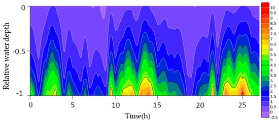
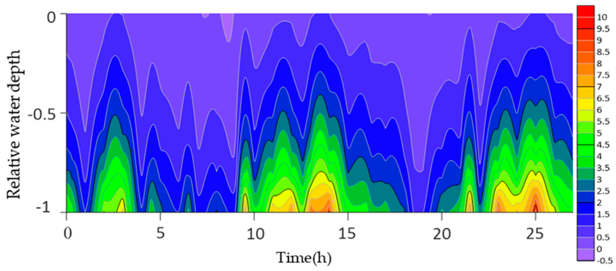
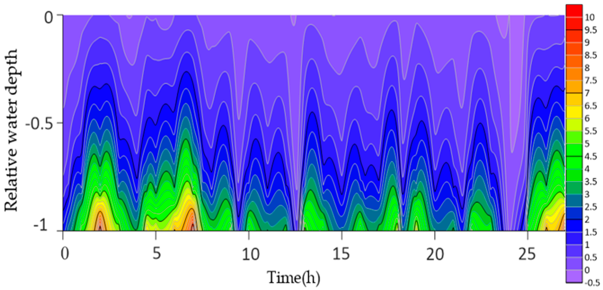
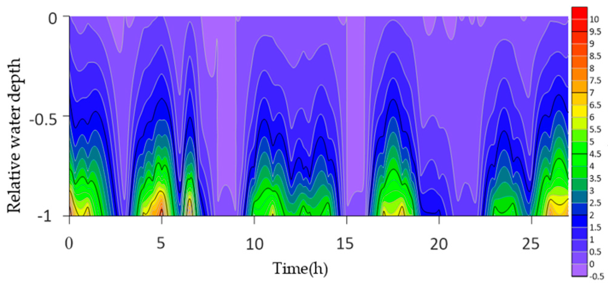
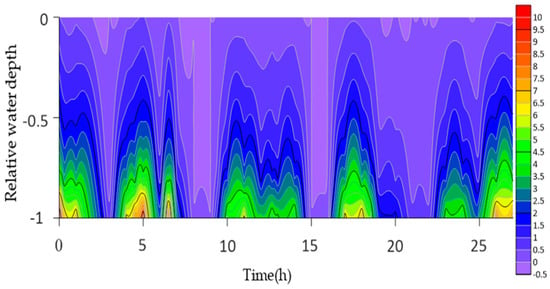
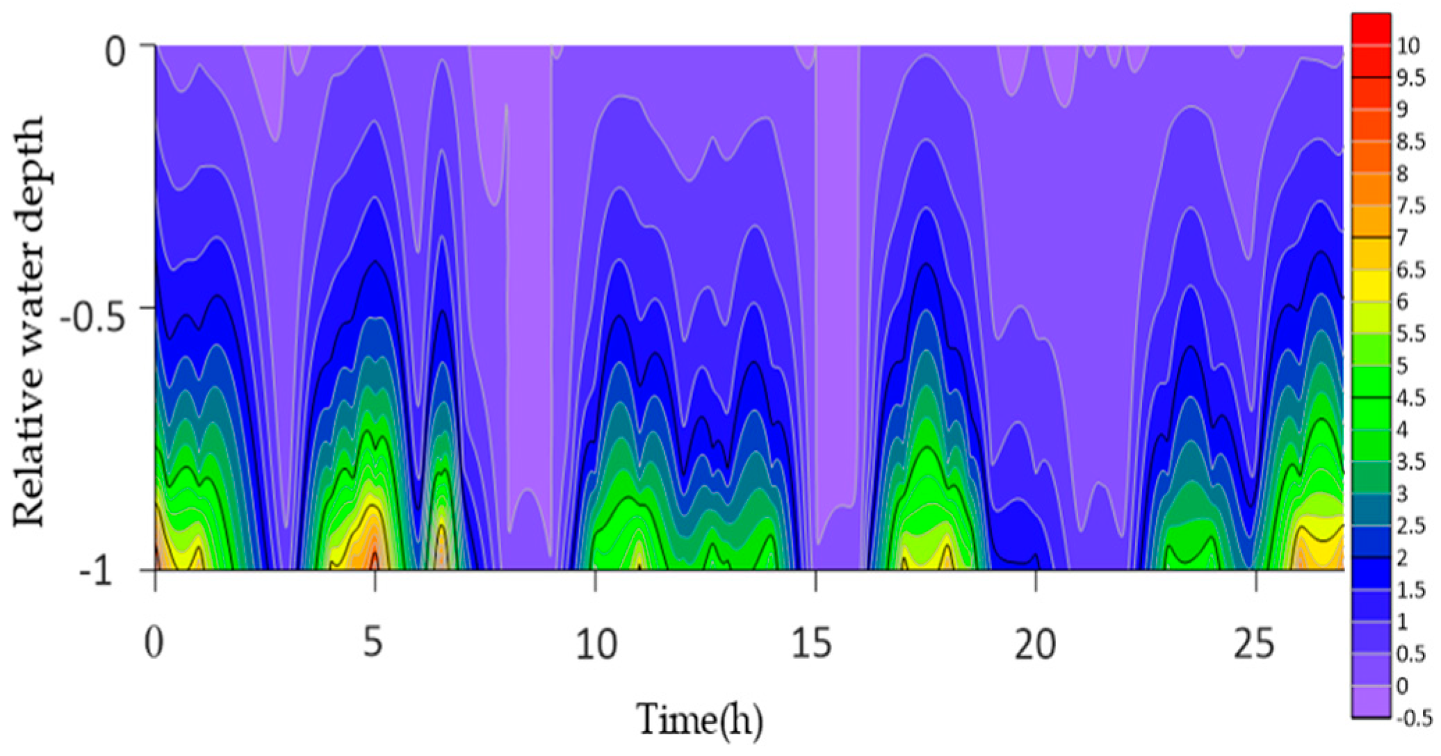
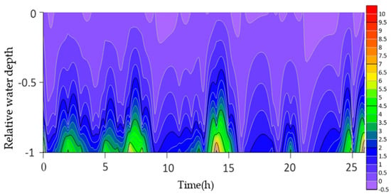
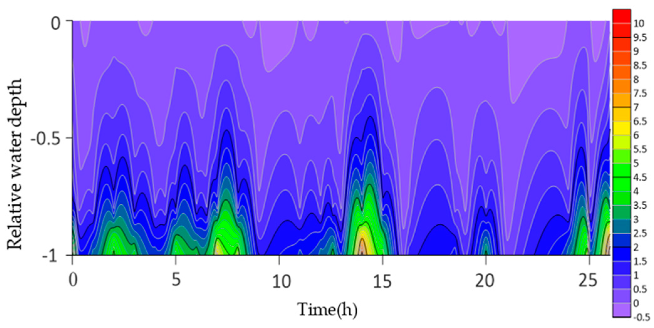
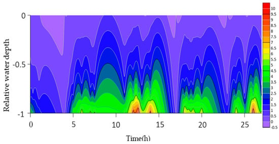
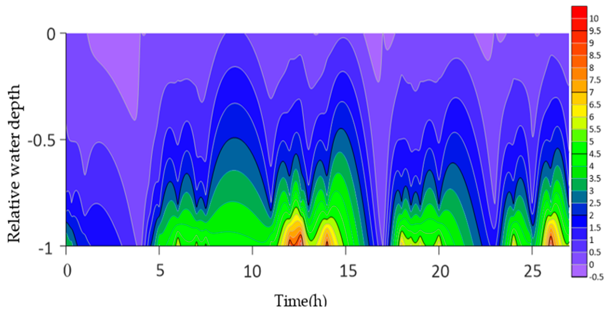
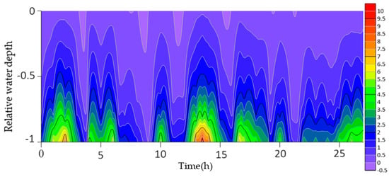
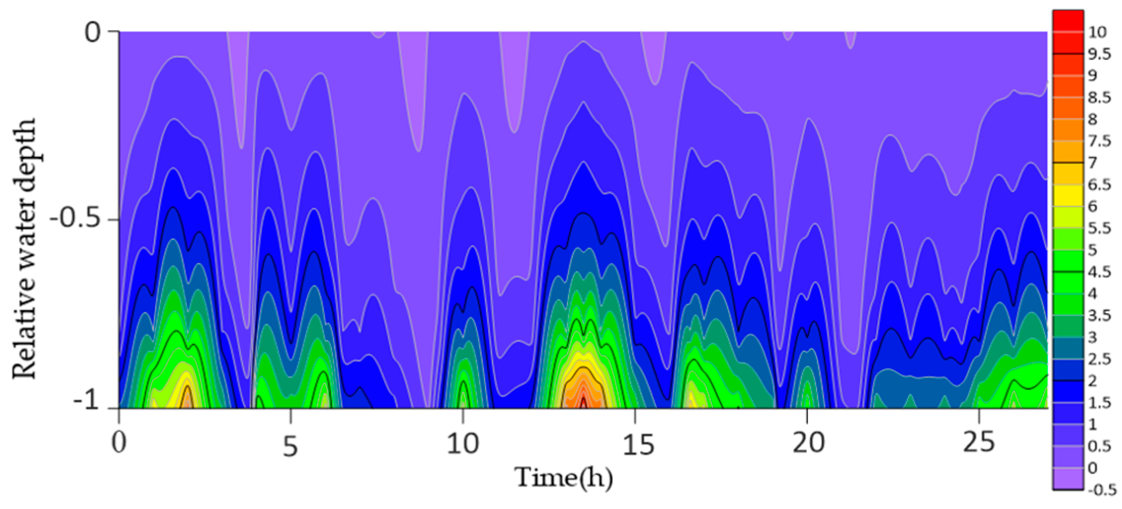
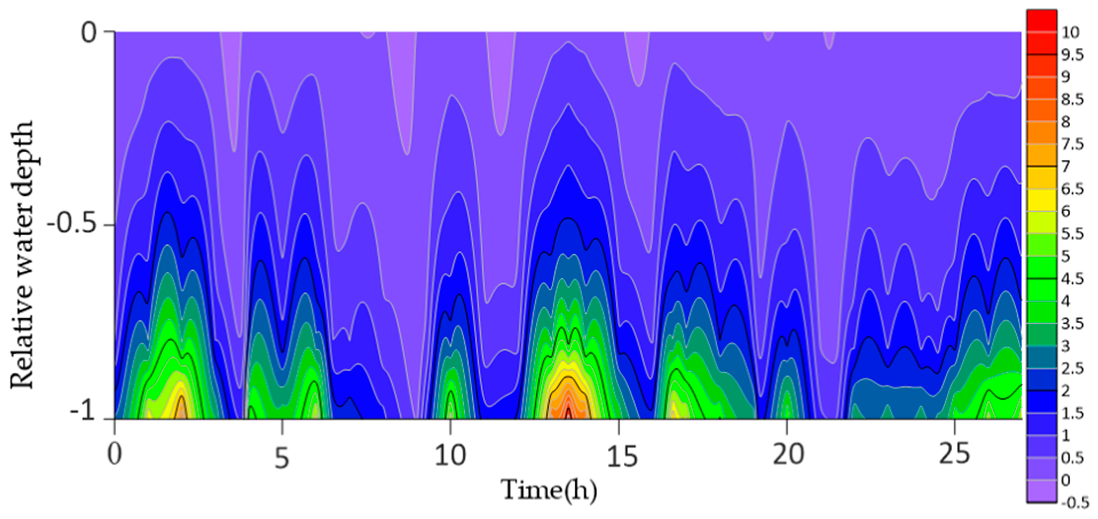
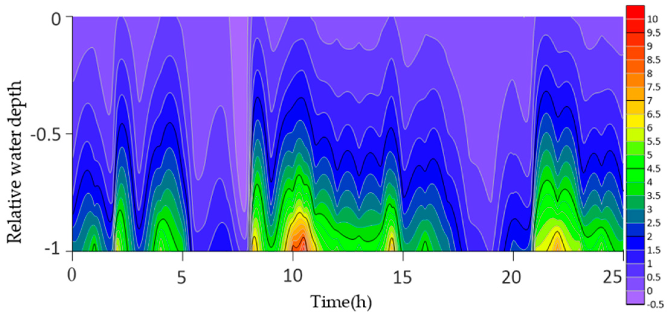
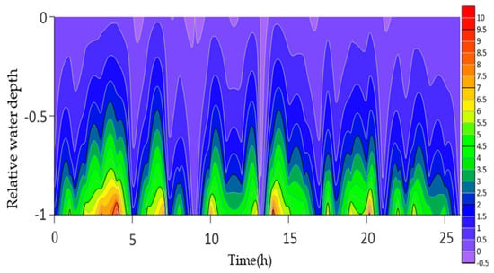
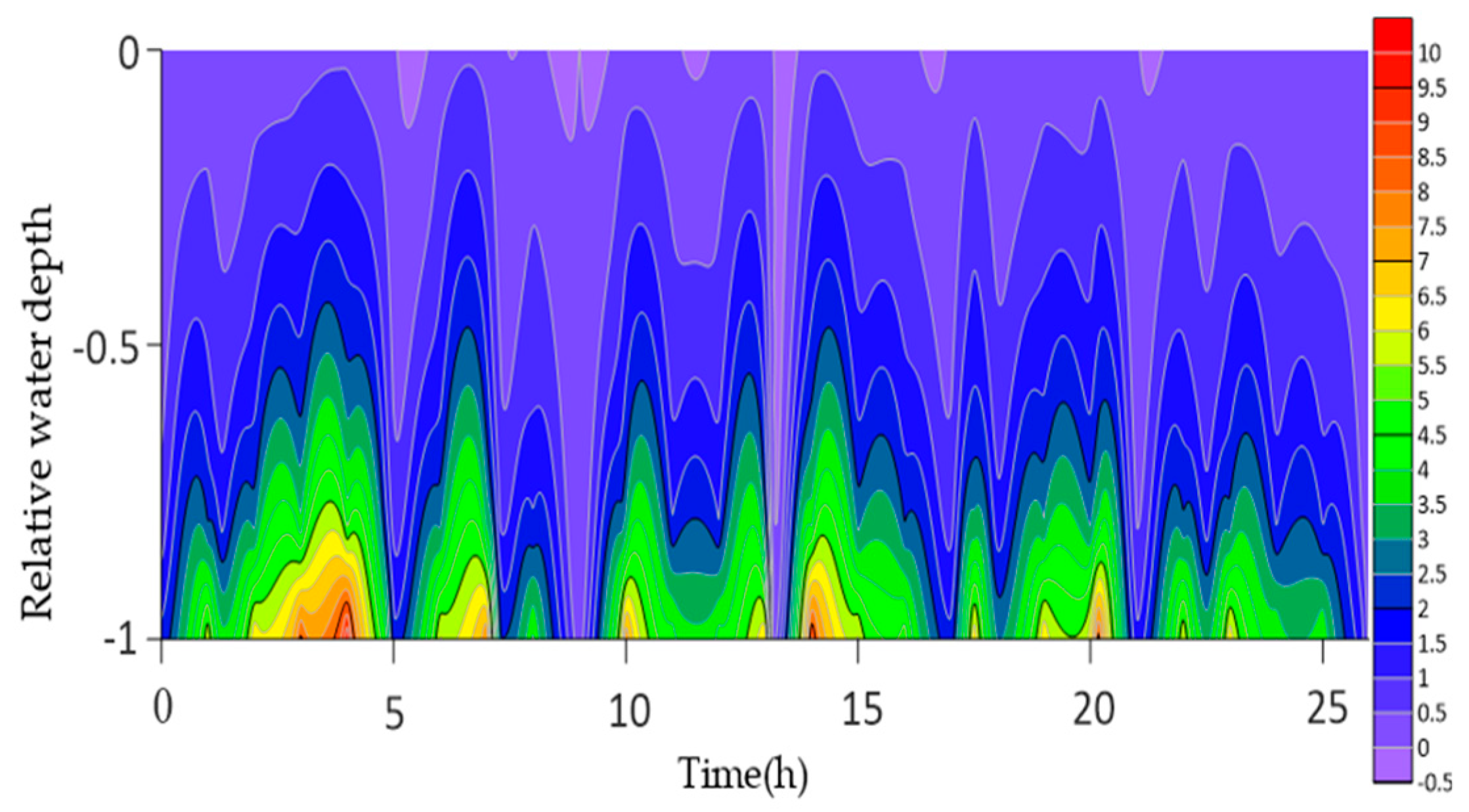
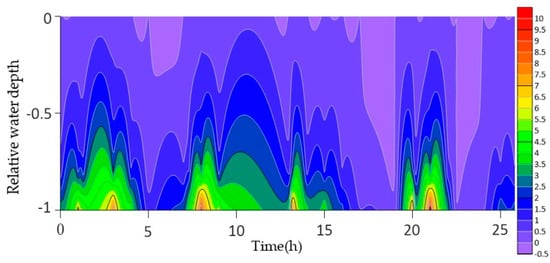
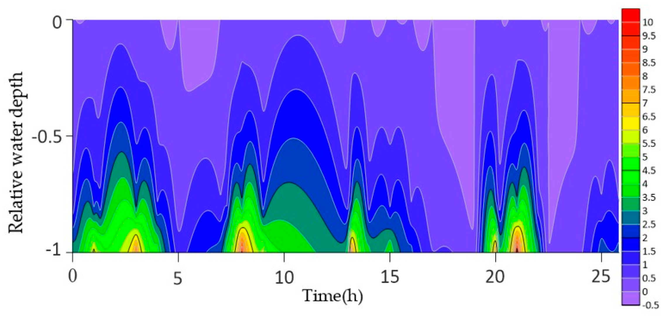
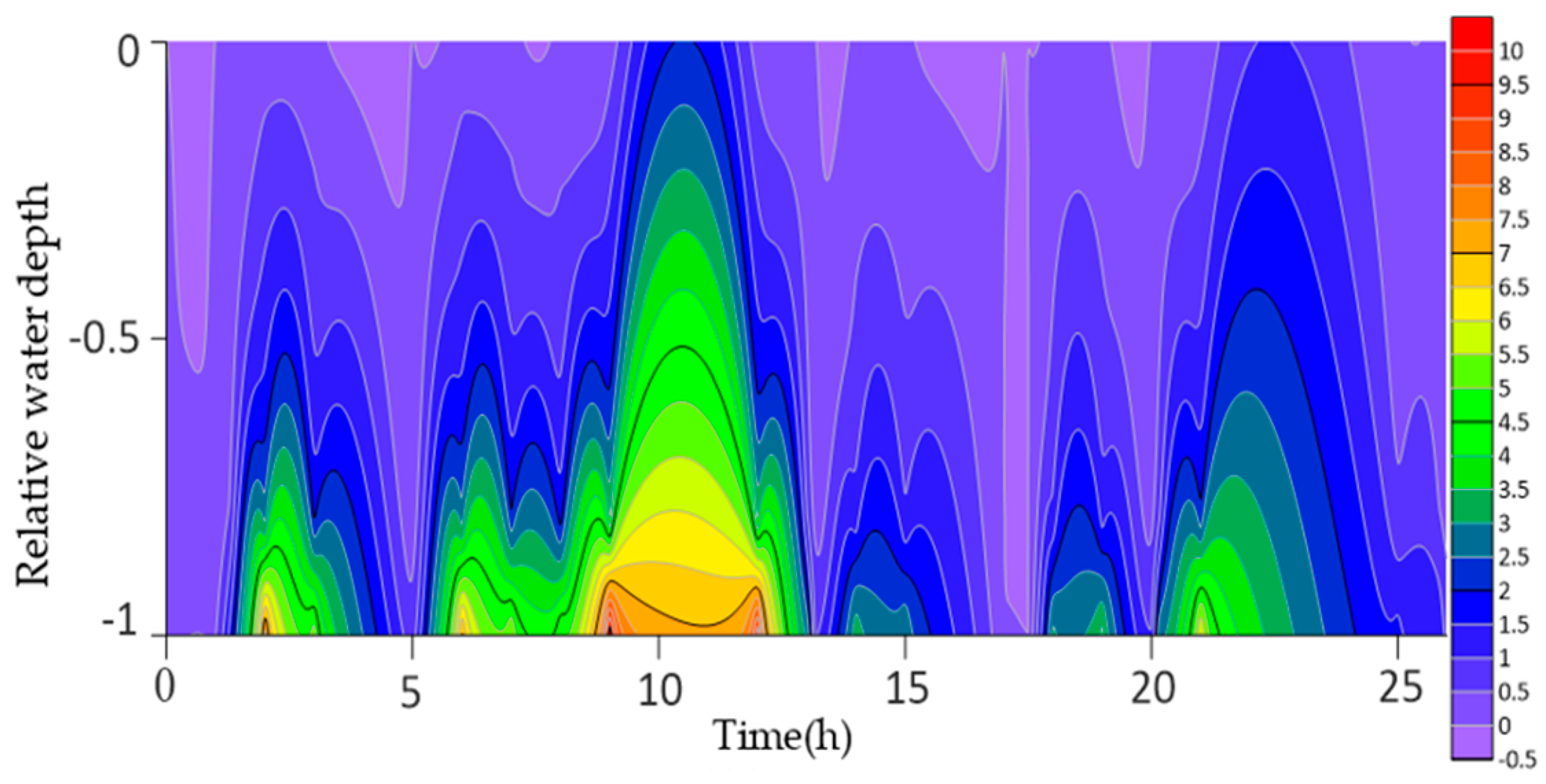
The spatial distribution of the sampling stations is illustrated in Figure 2. Temporal variations in turbulent shear at each station are shown in Figure 2, Figure 3, Figure 4, Figure 5, Figure 6, Figure 7, Figure 8, Figure 9, Figure 10, Figure 11, Figure 12 and Figure 13.

Figure 2. Turbulent shear at Station A (25 April 2016).

Figure 3. Turbulent shear at Station B (25 April 2016).

Figure 4. Turbulent shear at Station C (25 April 2016).

Figure 5. Turbulent shear at Station D (25 April 2016).

Figure 6. Turbulent shear at Station D (25 April 2016).

Figure 7. Turbulent shear at Station F (25 April 2016).

Figure 8. Turbulent shear at Station A (30 April 2016).

Figure 9. Turbulent shear at Station B (30 April 2016).

Figure 10. Turbulent shear at Station C (30 April 2016).

Figure 11. Turbulent shear at Station D (30 April 2016).

Figure 12. Turbulent shear at Station E (30 April 2016).

Figure 13. Turbulent shear at Station F (30 April 2016).

The vertical distributions of turbulent shear G, derived from the velocity profiles, are illustrated in Figure 2. Turbulent shear at Station A (25 April 2016). Across the water column, G generally ranges from −0.5 s⁻¹ to 10 s⁻¹. Negative values mainly occur during periods of very weak turbulence, such as near-surface conditions under calm winds or around slack tide when velocity gradients are minimal. These conditions indicate weak vertical mixing and relatively stable stratification, which may reduce sediment resuspension.

In general, turbulent shear tends to be stronger near the bed than near the surface, reflecting enhanced turbulence generated by bottom friction. For most observation periods, G varies primarily between 0 s⁻¹ and 7 s⁻¹. Another noticeable feature is the occurrence of mid-tide peaks in G during the observation period. These peaks generally correspond to periods of higher current velocity, suggesting that variations in turbulent shear are closely associated with changes in flow speed.

3. Results

Spatiotemporal Patterns of Suspended Sediment Concentration in the Guan River Estuary

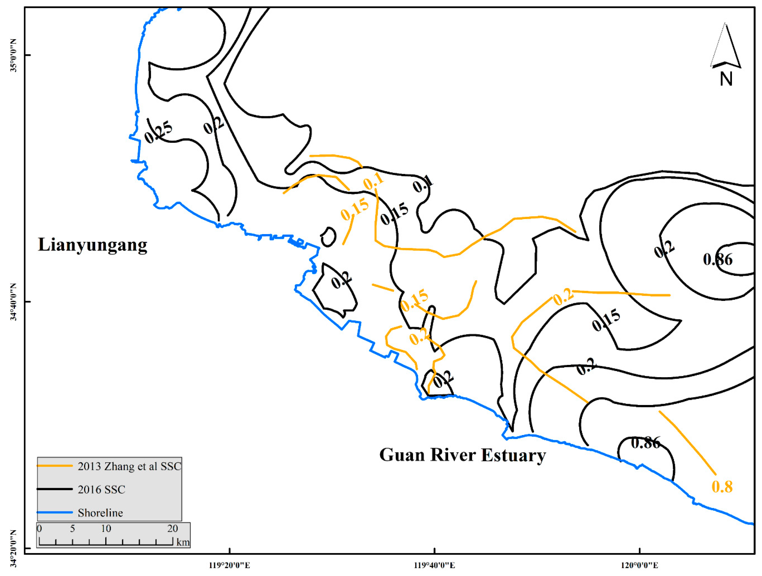
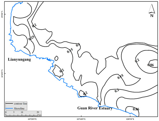
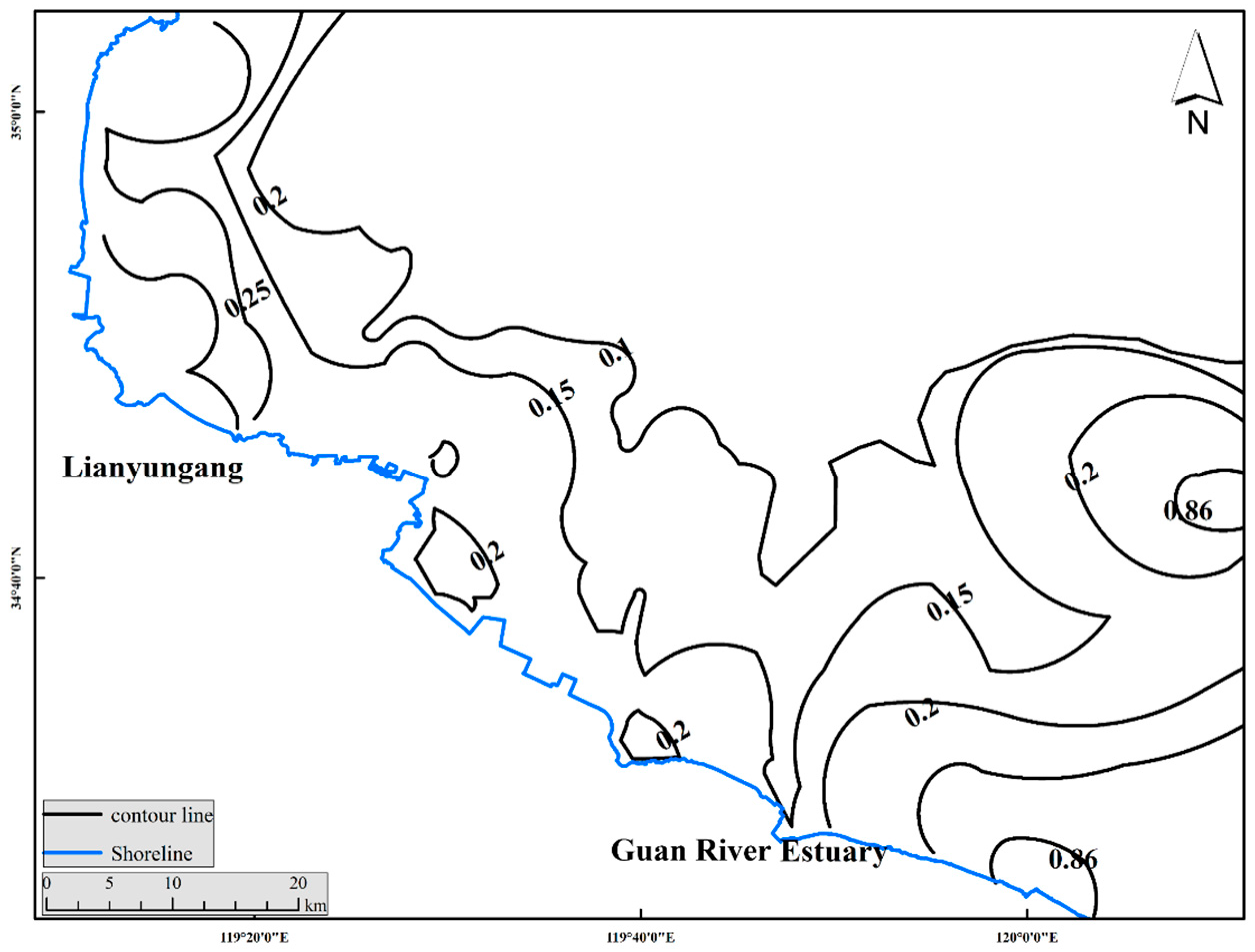
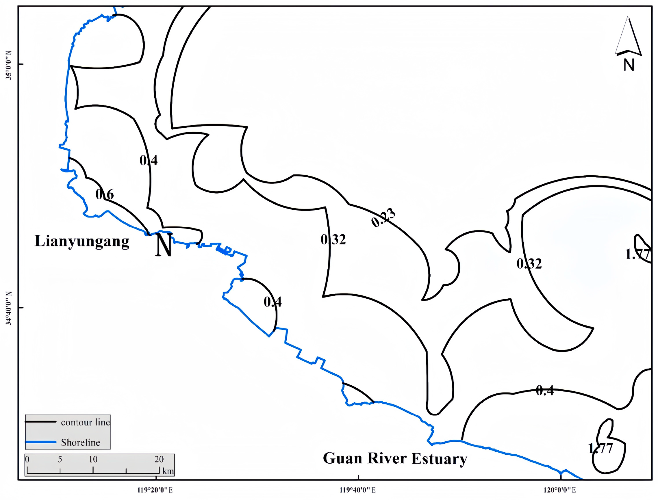
Using Equation (9), suspended sediment concentration (SSC) was retrieved from remote sensing imagery, and an SSC contour map for the river–sea junction was generated (Figure 14). The selected imagery corresponds to warm season conditions during neap tide and ebb tide. The results show a clear spatial pattern characterized by higher SSC near the coast and lower values offshore, with offshore contours generally parallel to bathymetric contours.

From a seasonal perspective, SSC in warm season is lower than in other, consistent with previous studies [15,16,17,18] that attribute this pattern to the seasonal variability of the western Yellow Sea coastal current. Compared with the annual mean SSC distribution reported by Zhang Tingrong et al. [19], the warm season retrievals are slightly lower. For example, east of the Guanhe Estuary, the annual mean SSC contour of 0.2 kg/m³ corresponds to approximately 0.15 kg/m³ in warm season, and near the Lezihe Estuary, the spatial extent of the 0.2 kg/m³ contour is substantially smaller in warm season. Overall, the SSC distribution exhibits an east–west gradient, with higher concentrations in the east and lower concentrations in the west. The highest SSC occurs east of the Guanhe Estuary (up to 0.86 kg/m³) and decreases toward the Lianyungang coastal waters (down to approximately 0.15 kg/m³), while relatively high SSC values are also observed near the Lezihe Estuary and the nearshore waters of Lianyungang.

Figure 14. Contour plot of surface sediment concentration. The plotting method is similar to that described in Zhang et al. (2013) [19].

Figure 14. Contour plot of surface sediment concentration. The plotting method is similar to that described in Zhang et al. (2013) [19].

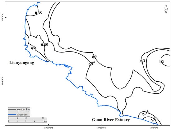
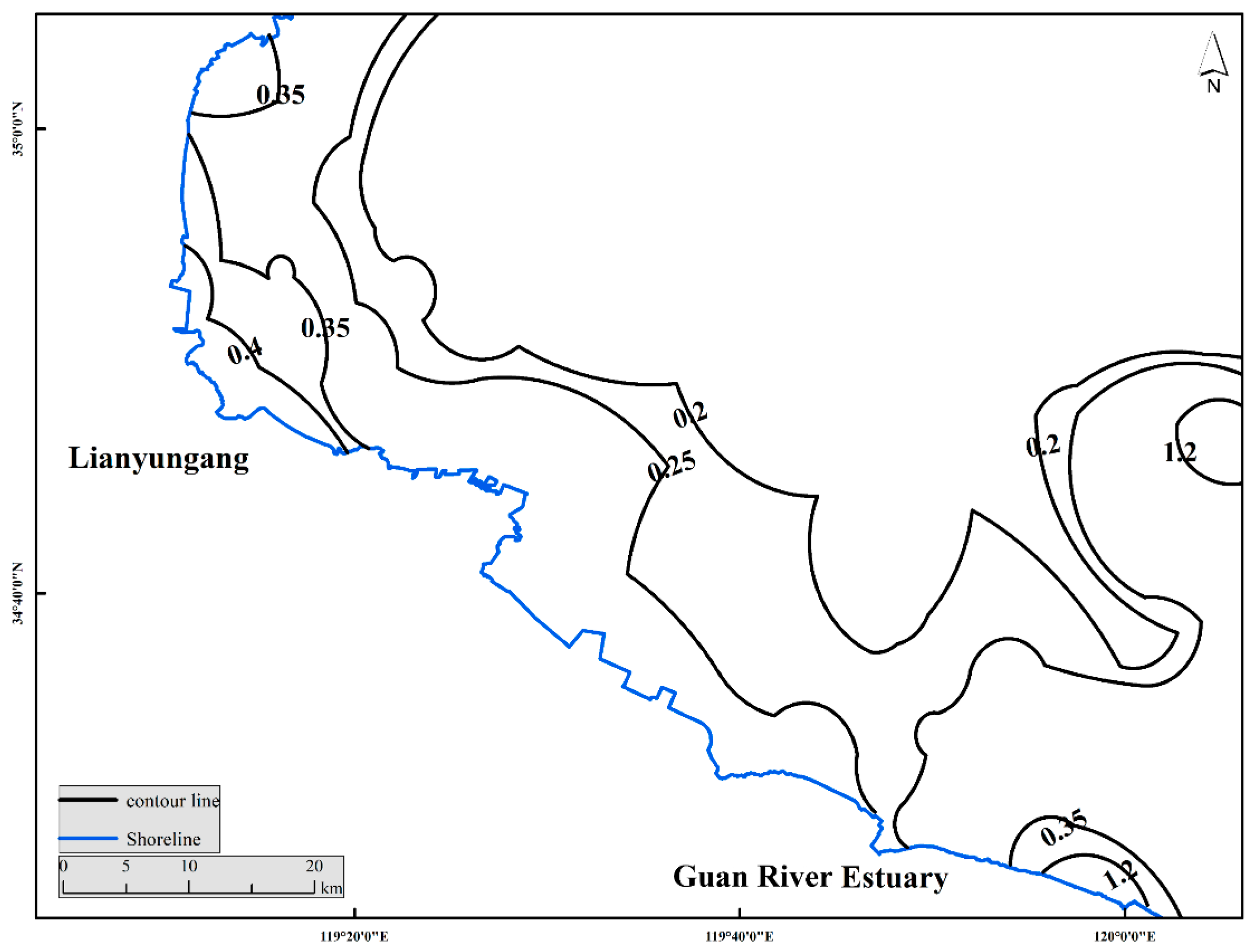
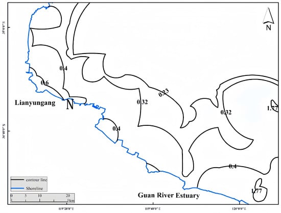
Based on the overall regression relationship, the vertical function corresponding to the neap-tide period that matches the satellite observation time was selected. Station E, which showed a similar surface suspended sediment concentration to that derived from the remote sensing image, was chosen to determine the corresponding water depth and flow velocity conditions. Using the surface SSC obtained from the satellite inversion, sediment concentrations in the middle and bottom layers were further estimated through profile fitting. Based on these calculations, contour maps of SSC for the surface, middle, and bottom layers in the river–sea transition zone of Haizhou Bay during the warm-season neap tide were generated (Figure 15, Figure 16 and Figure 17).

Figure 15. Contour map of surface suspended sediment concentration derived from remote sensing.

Figure 16. Contour map of middle-layer suspended sediment concentration derived from remote sensing.

Figure 17. Contour map of bottom suspended sediment concentration derived from remote sensing.

From a temporal perspective, suspended sediment concentrations are relatively high during the warm season, and clear vertical stratification can be observed. Surface SSC is markedly lower than that in the bottom layer, where the concentration is approximately twice that of the surface layer. This pattern is related to the prevailing southeasterly winds along the Jiangsu coast during the warm season, which drive coastal currents from the southeast toward the northwest and promote the accumulation of suspended sediment in nearshore waters. Meanwhile, the weakening of vertical mixing under these wind conditions reduces sediment resuspension by tidal currents. In addition, higher water temperatures during the warm season decrease seawater viscosity and enhance sediment settling, contributing to higher concentrations in the lower water column.

Spatially, the middle and bottom layers display a distribution pattern characterized by higher concentrations in the eastern part and lower values in the western area, indicating a general transport tendency from the Guan River Estuary toward Lianyungang waters. The SSC contour lines roughly follow the bathymetric trend. In particular, the shoal area east of the Guan River Estuary exhibits a high-concentration zone in both the middle and bottom layers, similar to that observed at the surface. Overall, suspended sediment in the river–sea transition zone shows a clear spatial gradient, with higher concentrations near the coast than offshore, while vertically the concentration generally increases from the surface toward the seabed.

4. Discussion

4.1. Results of the Remote Sensing Inversion Models

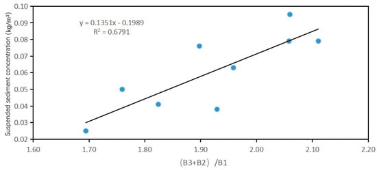
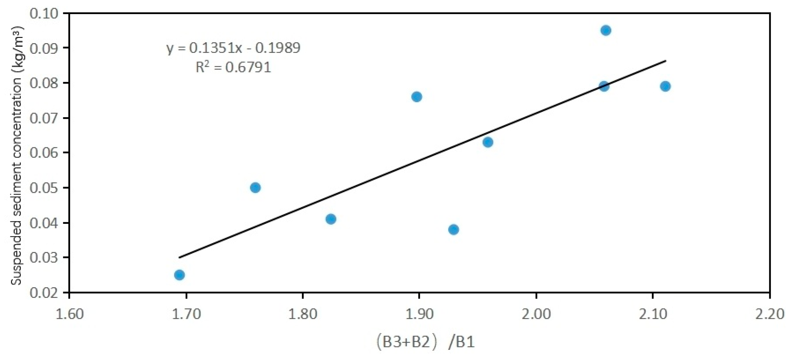
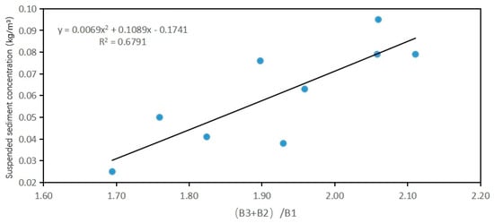
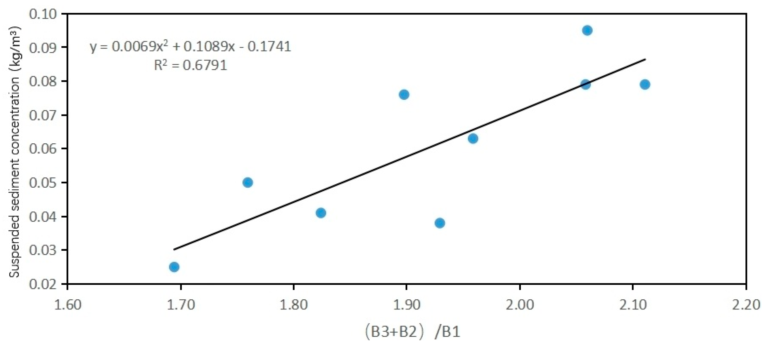
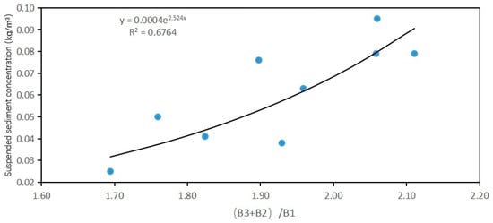
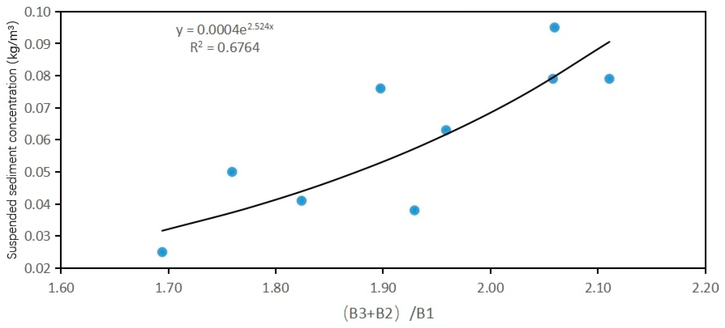
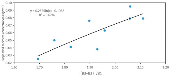
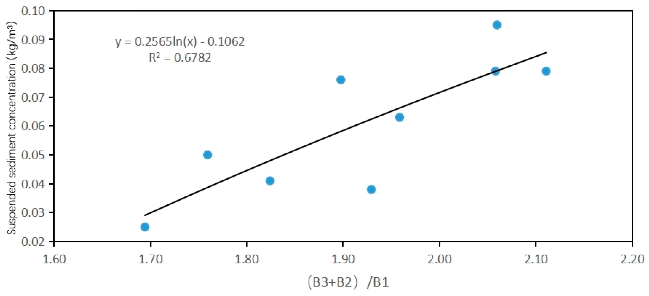
Regression relationships between the measured suspended sediment concentration (SSC) and various spectral band ratios were established to develop the inversion models. Among the tested models, those with correlation coefficients greater than 0.66 were considered to show relatively strong correlations. The corresponding fitting relationships and trend lines are illustrated in Figure 18, Figure 19, Figure 20 and Figure 21.

Figure 18. The combined values of (B3 + B2)/B1 band and the concentration value of suspended sediment were fitted to the trend line by a linear model.

Figure 19. The combined values of (B3 + B2)/B1 bands and the polynomial model of suspended sediment concentration values fit the trend line.

Figure 20. The combined value of (B3 + B2)/B1 band and the exponential function model of suspended sediment concentration value fit the trend line.

Figure 21. The combined value of (B3 + B2)/B1 band and the logarithmic function model of suspended sediment concentration value fit the trend line.

In summary, the inversion models with correlation coefficients higher than 0.66 for the river–sea transition zone are summarized in Table 25. The results indicate that both the linear model and the quadratic polynomial model based on the combination of Bands B1, B2, and B3 achieve the highest inversion accuracy. Considering the stability of the fitting relationship, the quadratic polynomial model derived from the ratios of these three bands was selected as the optimal model for estimating suspended sediment concentration in the study area. The corresponding equation is expressed as follows.

$$y=0.0069x^2+0.1089x-0.1741$$

(9)

Table 25. Function models with correlation coefficients higher than 0.66 and their correlation coefficients.

Band	Relation	${\mathit{R}}^2$
B2/B1	$y=0.8394x^2-0.9652x+0.2558$	0.66
B3/B1	$y=0.1753x-0.1208$	0.6604
	$y=0.01764x^2+0.13935x-0.10263$	0.6604
	$y=0.0019e^{3.2956x}$	0.6662
(B3+B2)/B1	$y=0.1351x-0.1989$	0.6791
	$y=0.0069x^2+0.1089x-0.1741$	0.6791
	$y=0.0004e^{2.524x}$	0.6764
	$y =0.2565\ln \left(x\right)-0.1062$	0.6782

In this model, $\mathrm{x}$ denotes the band ratio (B3 + B2)/B1. The correlation coefficient reaches 0.679, suggesting a relatively strong relationship.

4.2. Application of the Improved SSV Equation in the Guan River Estuary

To account for the influence of flocculation on sediment settling velocity (SSV), Van Leussen [20] proposed a formulation in which the settling velocity in still water is adjusted by introducing two turbulence-related factors: a growth term associated with aggregation and a disruption term related to turbulent break-up:

$${\omega }_s=k{C}^x\left(1+aG\right)/\left(1+b{G}^2\right)$$

(10)

where ω_s is the sediment settling velocity; k is an empirical constant; C is suspended sediment concentration; G is the root-mean-square velocity gradient; and a and b are empirically determined constants. Equation (10) was initially proposed by Argaman and Kaufman [21] and represents a simplified form of their original formulation. This equation fully accounts for the combined influence of SSC and turbulence on SSV; however, its nonlinear structure limits computational efficiency and parameter stability in regression-based applications.

For practical application, Equation (10) is further simplified as:

$${\omega }_s=k{C}^x{G}^y$$

(11)

where x and y are empirical constants. This simplification is justified by both physical reasoning and statistical testing: under well-mixed tidal conditions, the dominant effects of SSC and turbulence on flocculation can be effectively represented by power-law relationships, while higher-order nonlinear terms contribute marginally. Sensitivity analysis and regression testing confirmed that the simplified form retains comparable predictive performance while improving model robustness and computational efficiency.

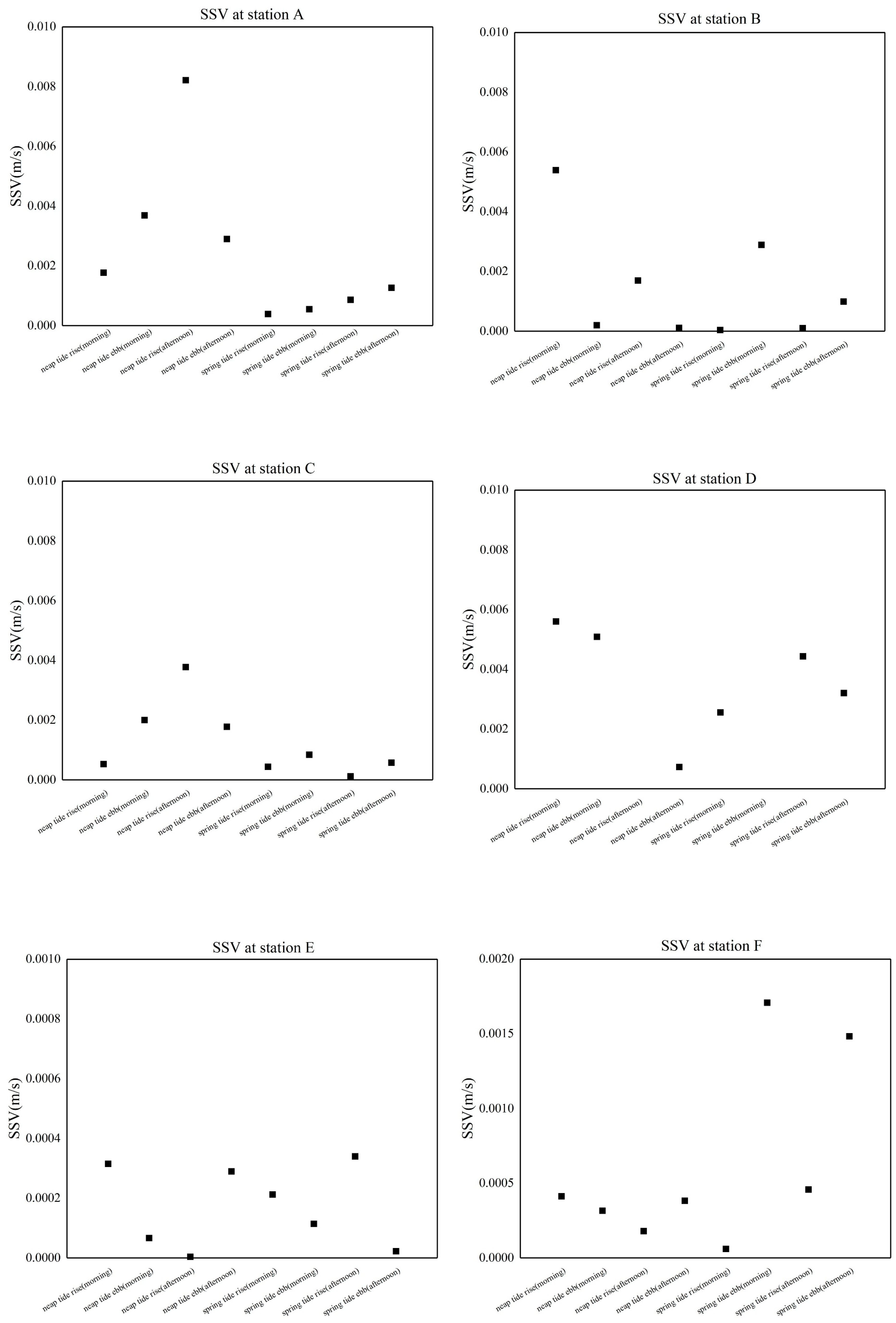
The SSV estimated by the Rouse equation varied from 0.000003 m/s to 0.0149 m/s throughout the study period. In order to study the relationship between turbulent shear and SSV in Guan River Estuary, the SSV is calculated by using the sediment concentration data during the spring tide and neap tide. The corresponding average SSV values at high and low water levels are presented in Figure 22. The results show that SSV during spring tides is generally lower than that observed during neap tides. During spring tides, an increase in turbulence intensity tends to reduce the settling velocity.

Figure 22. Tidal variation in SSV at each station.

The sediment concentration data and turbulence intensity data of six actual sites in Guan River Estuary in April 2016 were fitted with Equation (10), and nonlinear regression analysis was carried out to obtain the following best fitting values, as shown in Table 26.

Table 26. Regression coefficient and other related variables of fitting Equation (10).

	k	x	y	R2
spring tide	−0.55966	−0.11049	0.92509	0.6122
neap tide	−1.00776	−1.3826	0.83908	0.6796

Equation (10) can be expressed as follows:

$$\mathrm{Spring} \mathrm{tide}: {\omega }_s=-0.55966C^{-0.11049}{G}^{0.92509}$$

(12)

$$\mathrm{Neap} \mathrm{tide}: {\omega }_s=-1.00776C^{-1.3826}{G}^{0.83908}$$

(13)

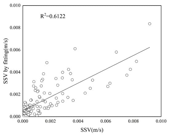
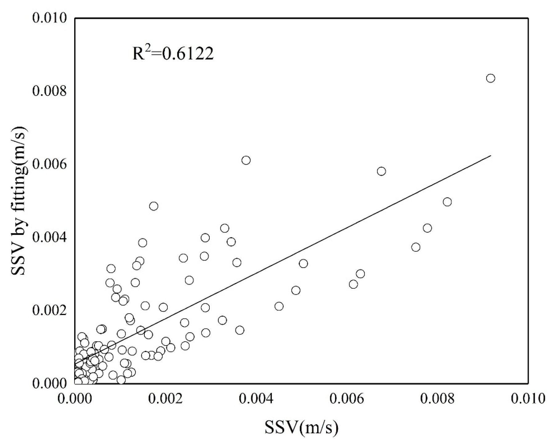
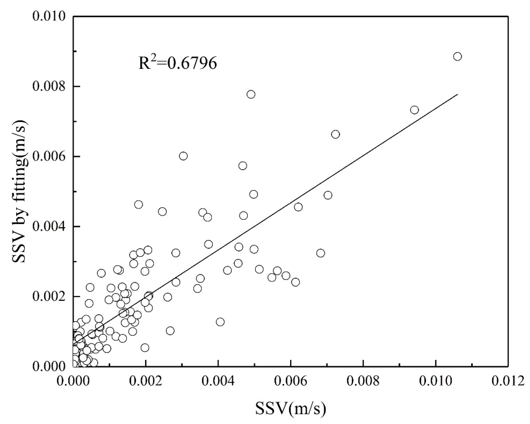
Equation (10) was applied to estimate the SSV during both spring and neap tides. The relationship between the calculated SSV and the fitted SSV is illustrated in Figure 23 and Figure 24.

Figure 23. The correlation between the SSV and the SSV by fitting in spring tide period.

Figure 24. The correlation between the SSV and the SSV by fitting in neap tide period.

4.3. Sediment Settling Velocity and Its Controls in the Guan River Estuary

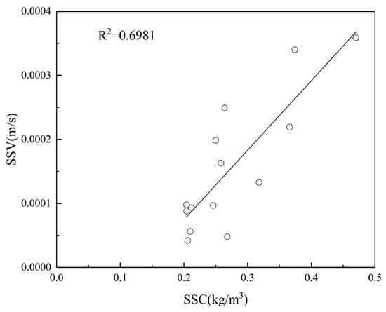
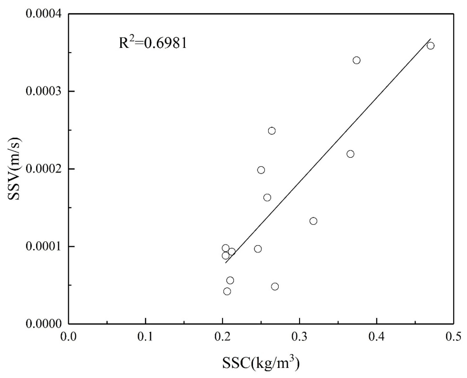
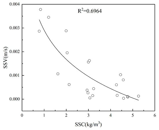
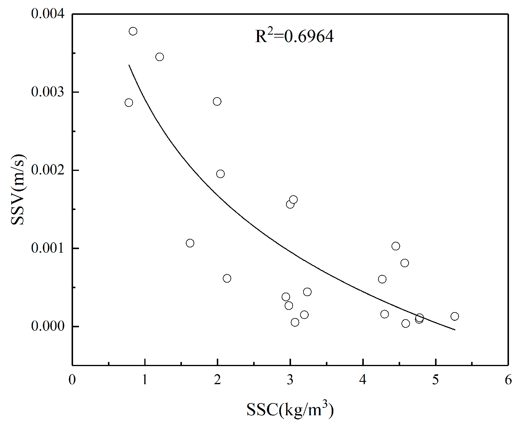
Analysis of sediment data from each station shows that the relationship between sediment settling velocity (SSV, ω_s) and suspended sediment concentration (SSC) is nonstationary. At station E, where SSC is relatively low (approximately 0.15–0.45 kg/m³), SSV is positively correlated with SSC (Figure 25), with a coefficient of determination of R² = 0.6981. In contrast, at station C, where SSC is higher (approximately 0.8–5.5 kg/m³), SSV exhibits a negative correlation with SSC (Figure 26), with R² = 0.6964, indicating sedimentation hindrance under high-concentration conditions.

Figure 25. The variation in SSV with SSC at station E.

Figure 26. The variation in SSV with SSC at station C.

These contrasting behaviors reflect the competing influences of flocculation and hindered settling. At low SSC, fine particles tend to aggregate into flocs through inter-particle collisions enhanced by turbulence, resulting in increased effective particle size and, consequently, higher settling velocities. Similar flocculation-enhanced settling behavior has been reported in estuarine and coastal environments, including the Yangtze River Estuary and adjacent nearshore waters [22,23]. As SSC increases beyond a threshold, a space-filling floc network forms, leading to increased inter-particle interference and reduced settling efficiency, thereby causing SSV to decrease with further increases in SSC.

The coupling between SSV, turbulence, and flocculation is further supported by theoretical and experimental studies. Van Leussen [20] demonstrated that turbulence intensity, commonly quantified by the root-mean-square velocity gradient G, controls both floc growth and breakup, thereby regulating settling velocity. Similarly, Winterwerp [24] showed that the balance between turbulent shear-induced aggregation and disruption governs floc size evolution and settling behavior. In the present study, the observed SSC-dependent variation in SSV across stations reflects spatial differences in turbulence intensity and sediment concentration, highlighting the combined role of hydrodynamic forcing and particle interactions in regulating vertical sediment transport.

5. Conclusions

This study combines Landsat 8 remote sensing images with measured suspended sediment concentration data. Taking the single band of remote sensing images and various combinations of different bands as independent variables and the measured suspended sediment concentration as the dependent variable, the inversion relationship of suspended sediment concentration under various functional model relationships is established.

A new formula for the period of low tide that is consistent with remote sensing images was selected. Through the surface sediment concentration inversion by remote sensing, the sediment concentration fields of the middle layer and the bottom layer were fitted. Through formula fitting, it was found that the sediment concentrations of both the middle layer and the bottom layer showed a characteristic of being higher in the east and lower in the west. The phenomenon of a high concentration field still occurred in the shallow beach on the east side of the Guanhekou River.

At the same time, improvements are proposed for the existing model for calculating the vertical distribution of suspended sand. It is suggested that the turbulent shear G be used to replace the physical quantities related to flow velocity in the original formula. A new formula for vertical sediment concentration was obtained by using the method of multiple linear regression, and the sedimentation characteristics of suspended sediment in estuaries were studied.

The main findings are as follows:

• A new equation of vertical sediment concentration is obtained using the multiple linear regression method:

$$\ln c={\alpha }_0+{\alpha }_1\ln \left(h-z\right)/z+{\alpha }_2\ln c_{\alpha }+{\alpha }_3\ln G$$

$$\mathrm{Spring} \mathrm{tide}: \ln c=-0.55966-0.11049\ln (h-z)/z+0.92509\ln c_a+0.06188\ln G$$

$$\mathrm{Neap} \mathrm{tide}: \ln c=-1.00776-1.38260\ln (h-z)/z+0.83908\ln c_a+0.05137\ln G$$

SSC at the river–sea confluence shows a clear spatial gradient, with higher values in nearshore areas and lower values offshore. The sediment concentration contours are generally parallel to the local isobaths. Surface SSC on the shoal east of the Guan River Estuary is noticeably higher than that on the western side, decreasing from approximately 0.86 kg/m³ in the east to 0.15 kg/m³ in the west.

Model fitting results indicate that this east–west contrast persists in deeper layers. Using the improved equation together with the remote-sensing-derived surface SSC during the neap tide period, the sediment concentration fields in the middle and bottom layers were estimated. High-concentration zones remain evident over the eastern shoal. The maximum SSC reaches about 1.2 kg/m³ in the middle layer and 1.77 kg/m³ near the bottom.

Temporal analysis suggests that pronounced sediment stratification occurs in the high-concentration region east of the estuary during the warm season. Surface concentrations are substantially lower than those near the bed, with bottom SSC values roughly twice those observed at the surface. Spatially, both the middle and bottom layers maintain the same pattern of higher concentrations in the east and lower concentrations in the west.

2.

The measured data are used to fit the SSV equation ${\omega }_s=a{C}^x{G}^y$, and the equations for the spring tide period and the neap tide period are also obtained:

$$\mathrm{Spring} \mathrm{tide}: {\omega }_s=-0.55966C^{-0.11049}{G}^{0.92509}$$

$$\mathrm{Neap} \mathrm{tide}: {\omega }_s=-1.00776C^{-1.3826}{G}^{0.83908}$$

The analysis of sediment settling velocity indicates that flocculation plays an important role in controlling particle settling. Flocculation is affected by several environmental factors, including suspended sediment concentration (SSC), turbulent shear, and salinity gradients. Because salinity data were not available in the present dataset, its influence was not included in the model. Incorporating salinity effects in future investigations may help improve model performance.

References

- Williamson, A.-N.; Grabau, W.-E. Sediment Concentration Mapping in Tidal Estuaries; NASA, Goddard Space Flight Center: Washington, DC, USA, 1973. [Google Scholar]
- Curran, P.J.; Novo, E.M.M. The relationship between suspended sediment concentration and remotely sensed spectral radiance: A review. J. Coast. Res. 1988, 4, 351–368. [Google Scholar]
- Nechad, B.; Ruddick, K.G.; Park, Y. Calibration and validation of a generic multisensor algorithm for mapping of total suspended matter in turbid waters. Remote Sens. Environ. 2010, 114, 854–866. [Google Scholar] [CrossRef] [Scilit]
- Zhen, H. Research on Remote Sensing Information Extraction and Quantitative Inversion of Suspended Sediment in Coastal Zone Muddy Tidal Flats and Class II Water Bodies; East China Normal University: Shanghai, China, 2004. [Google Scholar]
- Pan, J.L.; Guo, B.Y. Remote Sensing Study on Suspended Sediment Concentration in Zhoushan Archipelago Sea Area Based on Landsat8 Data. Mar. Dev. Manag. 2020, 37, 82–90. [Google Scholar] [CrossRef]
- LIU, Q.; Rossiter, D.G. Estimation of Suspended Sediment Concentration in Poyang Lake Using MODIS and Hyperspectral Data. Remote Sens. Technol. Appl. 2008, 23, 7–11. [Google Scholar]
- Yang, H.; Mei, T.; Chen, X. Variation of Satellite-Based Suspended Sediment Concentration in the Ganges-Brahmaputra Estuary from 1990 to 2020. Remote Sens. 2024, 16, 396. [Google Scholar] [CrossRef] [Scilit]
- He, X.; Song, X.; Pang, Y.; Li, Y.; Chen, B.; Feng, Z. Distribution, sources, and ecological risk assessment of SVOCs in surface sediments from Guan River Estuary, China. Environ. Monit. Assess. 2014, 186, 4001–4012. [Google Scholar] [CrossRef] [Scilit] [PubMed]
- Zhang, L.; Lin, W.; Li, K.; Sheng, J.; Wei, A.; Luo, F.; Wang, Y.; Wang, X.; Zhang, L. Three-dimensional water quality model based on FVCOM for total load control management in Guan River Estuary, Northern Jiangsu Province. J. Ocean Univ. China 2016, 15, 261–270. [Google Scholar] [CrossRef] [Scilit]
- Huang, J.; Yin, Y.; Xu, J.; Zhu, X. Spatial distribution features and environment effect of heavy metal in intertidal surface sediments of Guanhe estuary, Northern Jiangsu Province. Front. Earth Sci. China 2008, 2, 147–156. [Google Scholar] [CrossRef] [Scilit]
- Pan, J.L. Research on the Distribution of Suspended Sediment in the Zhoushan Archipelago Sea Area Based on Remote Sensing Technology. Master’s Thesis, Zhejiang Ocean University, Zhoushan, China, 2020. [Google Scholar]
- Yuan, X.Z.; Fang, J.C. Improvement Ideas for the 50,000-ton Class Channel Improvement Project at Guanhekou. China Water Transp. Waterw. Sci. Technol. 2019, 6–12. [Google Scholar]
- Han, X.; Zhu, W.J.; Pan, X.S.; Wang, N.; Shi, M. Multiple linear regression analysis of vertical Distribution of nearshore suspended sediment. Mar. Bull. 2021, 40, 182–188. [Google Scholar]
- Camp, T.R.; Stein, P.C. Velocity gradients and internal work in fluid motion. J. Boston Soc. Civ. Eng. 1943, 30, 219–237. [Google Scholar]
- Huang, J. Inversion and Spatiotemporal Distribution of Suspended Sediment Concentration in Haibowan Reservoir Based on Multi-Source Remote Sensing Data. Master’s Thesis, Inner Mongolia Agricultural University, Hohhot, China, 2022. [Google Scholar]
- Zuo, S.; Pang, Q.; Yang, H.; Zhang, N. Analysis on distribution characteristics and movement law of suspended sediment in Haizhou Bay. J. Shandong Univ. Sci. Technol. 2013, 32, 10–17. [Google Scholar]
- Lu, P.; Yue, Y.; Zhu, L.; Hu, R.; Yin, Y.; Leng, X. Distribution, transport and controlling factors of suspended sediment in the coastal waters of Rizhao in the western South Yellow Sea. Mar. Geol. Quat. Geol. 2022, 42, 36–49. [Google Scholar]
- Su, Y.; Li, F.; Ma, H.; Qian, Q. Formation and seasonal variation of the bottom cold water mass in the northern East China Sea. J. Ocean. Univ. Qingdao 1989, 19, 1–14. [Google Scholar]
- Zhang, T.; Zhang, W.; Xie, M.; Huang, W. Numerical simulation and distribution characteristics of sediment concentration field in Lianyungang coastal waters. Guangdong Water Resour. Hydropower 2013, 10, 9–13. [Google Scholar]
- Van Leussen, W. Estuarine macroflocs and their role in fine-grained sediment transport. Cont. Shelf Res. 1994, 14, 1353–1370. [Google Scholar]
- Argaman, Y.; Kaufman, W.J. Turbulence and flocculation. J. Sanit. Eng. Division 1970, 96, 223–241. [Google Scholar] [CrossRef] [Scilit]
- Chen, S.L.; Gu, G.C.; Zhang, G.A. Estimation of suspended sediment settling velocity in nearshore waters of the South Branch of the Yangtze River Estuary. J. Sediment Res. 2003, 6, 45–51, (In Chinese with English abstract). [Google Scholar]
- Shi, Z.; Zhu, W.W.; Zhou, H.Q. Settling velocity of fine suspended sediment outside the North Channel of the Yangtze River Estuary. J. Shanghai Jiaotong Univ. 2000, 34, 18–23, (In Chinese with English abstract). [Google Scholar]
- Winterwerp, J.C. A simple model for turbulence-induced flocculation of cohesive sediment. J. Hydraul. Res. 1998, 36, 309–326. [Google Scholar] [CrossRef] [Scilit]
Disclaimer/Publisher’s Note: The statements, opinions and data contained in all publications are solely those of the individual author(s) and contributor(s) and not of MDPI and/or the editor(s). MDPI and/or the editor(s) disclaim responsibility for any injury to people or property resulting from any ideas, methods, instructions or products referred to in the content. |
© 2026 by the authors. Licensee MDPI, Basel, Switzerland. This article is an open access article distributed under the terms and conditions of the Creative Commons Attribution (CC BY) license.