


Abstract
Companies are under increasing legal and societal pressure to reduce CO2 emissions from their delivery vehicles, while maximizing profit remains their prime objective. We study a problem where a company sends engineers with vehicles to customer sites to provide services. Customers request the service at their preferred time windows through a website or by calling a call center, and the company needs to allocate these service tasks to time windows and decide on how to schedule these tasks among its vehicles. We propose an approach to this problem that applies low-emission vehicle-scheduling techniques with dynamic pricing to reduce CO2 emissions and maximize profit. When a customer requests a service with a preferred time window, the company will provide the customer with different service time window options and their corresponding prices. Incentives are included in the prices to influence the customers to reduce CO2 emissions. Our approach solves the problem in two phases: the first phase solves time-dependent vehicle scheduling models with the objective of minimizing CO2 emissions, and the second phase solves a dynamic pricing model to maximize profit. Results show that our approach significantly reduces CO2 emissions and increases profits. A GenAI-based interpretation tool is used to translate the optimization outputs into actionable guidance for planners.
1. Introduction
Since the introduction of international agreements such as the Kyoto Protocol in 1998, companies have been under growing pressure to reduce carbon dioxide and other greenhouse gas emissions. Domestic transport in the UK accounted for around 29% of emissions in 2023, with road transport responsible for nearly 89% of this share [1], and in 2024, the sector’s share rose to 30%, even though overall transport emissions declined slightly [2]. The demand in the service delivery sector is also expanding rapidly. The UK’s on-demand home services market, including installations, repairs, and maintenance, is projected to grow at a CAGR of 9.06% between 2025 and 2034, reaching approximately USD 24.82 billion by 2035 [3]. Similarly, the field service management sector, which coordinates mobile engineers in industries such as utilities, telecoms, and appliance servicing, is expected to rise from USD 232.18 million in 2024 to USD 1060.12 million by 2034, at a CAGR of 16.4% [4]. The UK Climate Change Committee emphasizes that one-third of the required emissions cuts by 2040 must come from consumer behavior, including transport-related choices [5]. These trends highlight the dual challenge of meeting customer demand while reducing environmental impact and the need for solutions that not only reduce fleet emissions but also guide customers towards more sustainable decisions.
In this paper, we address the problem of services at customer sites located within a confined geographical area, so the differences in travel time are relatively small. However, the timing of travel plays a significant role, as it has a great impact on vehicle CO2 emissions. A key feature of the service considered in this paper is that scheduling is more critical than routing, especially since the engineers spend most of their time on service tasks and relatively little time on traveling between tasks. In confined urban areas, distances between customer sites are relatively short (e.g., no more than 5 miles) and engineers may often need to change travel path according to the real-time traffic/road condition or to drive a bit further for parking, so advanced routing choices contribute little variation to emissions. Instead, the timing of travel under congested traffic conditions has a much greater impact on fuel use and CO2 output. Incorporating detailed routing decisions would substantially increase the model’s complexity while adding little practical benefit in this context. By focusing on scheduling, the model remains computationally efficient for real-time decision support and is directly aligned with how companies interact with customers through time window bookings.
The VSP is used to allocate service tasks to the schedules of a fleet of vehicles initially located at a depot. Since traffic conditions have a significant influence on CO2 emissions, the amount of emissions generated and travel time per trip are modeled as being time-dependent to capture congestion patterns. Customer orders arrive dynamically, and each customer order comes with a preferred time window. A time window is a period within which the service must start, e.g., a two-hour time window of 8–10 a.m. We aim to schedule the service tasks and the vehicles’ travel to reduce CO2 emissions whilst maximizing profits by influencing customers’ choice of time windows through pricing incentives. The price will reflect the cost of the delivery option, which is calculated using the cost of CO2 emissions. As the cost of engineer wages is fixed, the only cost varying with the delivery option is the emission cost or fuel cost. A cost value is assigned to each kg of CO2 emissions. Environmental sustainability is a concern for all; thus, the discounted delivery windows will be tagged as green/environmentally friendly windows, showing the amount of emissions that can be saved by choosing such options, which may further influence customers to choose these windows.
This paper, therefore, proposes a two-phase decision-support framework that combines emission-aware scheduling with dynamic pricing. In the first phase, a new time-dependent vehicle-scheduling model minimizes CO2 emissions by accounting for congestion patterns. In the second phase, a dynamic pricing model offers customers differentiated time window options, with incentives to steer demand towards lower-emission slots, thereby maximizing profitability while promoting sustainability. Computational experiments simulating a service delivery company’s operation demonstrate that this approach can simultaneously reduce emissions and increase profitability. Real-time decision making is becoming increasingly important in service operations, and hence, we added a generative artificial intelligence (GenAI) interpretation component to help close the gap between complex optimization outputs and the information managers need by presenting results in a clear and practical form.
The rest of the paper is organized as follows. Section 2 reviews relevant literature on green scheduling and dynamic pricing. Section 3 presents the problem in detail and outlines the two-phase solution framework. Section 4 and Section 5 develop the mathematical models for scheduling and pricing, respectively. Section 6 reports numerical experiments and sensitivity analyses. Section 7 explains how GenAI can be used to interpret model outputs and enhance the framework’s role as a decision-support tool. Section 8 concludes with managerial implications and future research directions.
2. Literature Review
This study builds on three interconnected streams of research: (i) time-dependent green vehicle routing and scheduling problems, (ii) GenAI’s applications in logistics planning and optimization, and (iii) dynamic pricing in service and logistics contexts.
2.1. Time-Dependent Green Vehicle Routing and Scheduling Problems
Growing environmental regulations and societal concern over climate change have accelerated the adoption of sustainable logistics practices. As a result, the concept of green logistics and eco-efficient vehicle routing has gained prominence in both research and practice [6,7,8]. Early work in green routing mainly focused on minimizing travel distance as a proxy for emissions [9,10]. However, emissions are influenced not only by distance but also by factors such as vehicle load, speed, congestion, and technology. Studies such as Eglese and Black 2010 [11] highlighted that vehicle speed and congestion patterns are more critical than distance alone in estimating CO2 emissions. This has led to the development of time-dependent vehicle routing problems (TD-VRPs), where travel times and emissions vary depending on traffic conditions during the day.
Figliozzi [12] introduced emission-based routing using average travel speeds, showing that modest fleet adjustments could significantly reduce emissions. Jabali et al. [13] extended this by incorporating congestion periods into a time-dependent VRP, revealing trade-offs between emission reduction and travel time. Maden et al. [14] and Turkensteen [15] demonstrated the importance of realistic emission models to accurately capture fuel consumption and CO2 outputs. A comprehensive review by Demir et al. [16] categorized emission models from macro- to micro-scale, noting the widespread use of MEET, NAEI, and CEM models in routing studies.
2.2. GenAI Applications in Logistics Planning and Optimization
The rapid development of large language models (LLMs) within generative AI (GenAI) frameworks such as ChatGPT, Gemini, and Claude since the early 2020s has created new opportunities for organizations to embed AI-driven intelligence into business models and operational decision-making. GenAI has been widely explored as a productivity-improving technology across a broad range of domains, including marketing, healthcare, education, finance, retailing, and manufacturing [17].
In supply chain and logistics management, the adoption of AI and GenAI-supported techniques is also accelerating. For instance, generative adversarial networks have been applied to demand forecasting and inventory management, particularly in data-scarce environments, where their ability to generate realistic synthetic data improves forecast accuracy and safety stock decisions [18]. Similarly, recurrent neural networks have been used to support adaptive vehicle routing by capturing dynamic patterns in traffic congestion, vehicle capacity utilization, and demand fluctuations. Beyond predictive analytics, emerging paradigms such as digital twins and metaverse-based environments have been combined with GenAI tools to enhance decision-making in circular economy initiatives and sustainable operations [19].
Within logistics planning, GenAI has shown considerable capability in areas such as online customer interaction, supply chain visibility, and decision support for routing and scheduling [20]. However, as emphasized by Voß ([20]), GenAI tools remain limited as stand-alone decision-makers and achieve their greatest value when embedded within broader analytical or optimization-based systems such as simulation models, digital twins, heuristics, or mathematical programming frameworks. In the context of vehicle scheduling and dispatching, AI has therefore been primarily explored as a complementary technology, supporting tasks such as problem preprocessing, warm-start solution generation, heuristic operator selection, and population management in metaheuristic algorithms [21]. In a related stream, Yang et al. [22] argue that LLMs can be used as optimizers by translating natural-language problem descriptions into formal mathematical representations and potentially improving the balance between exploration and exploitation in solution search.
Despite these advances, the direct application of GenAI to vehicle routing and scheduling remains at an early stage. Zafar and Bayhan [23] investigated the use of LLM agents to solve two variants of the vehicle routing problem through prompt-based interaction. Their findings indicate that, while simpler problem instances could be handled, more complex variants, such as the electric vehicle routing problem, pose challenges due to issues including prompt sensitivity, verbose outputs, and hallucinated solutions. Chi et al. [24] proposed an LLM-assisted heuristic in which carefully designed prompts support the initialization, selection, mutation, and crossover stages of a differential evolution framework. Chen et al. [25] introduced an LLM-driven approach for task dispatching and navigation of autonomous vehicles, integrating LLMs into a reinforcement learning framework to support task interpretation, retrieval of historical execution records, and scheduling decisions. Addressing the limited ability of AI tools to capture complex interactions among decision variables in large-scale problems, Huang et al. [26] proposed a multimodal AI framework that combines textual and visual information to enrich prompt quality and improve optimization performance.
Overall, the literature suggests that GenAI currently delivers the greatest value in logistics planning as a supporting component within optimization-based decision-support systems, rather than as an autonomous solution generator. In addition, GenAI shows strong potential as an interpretive layer, translating complex optimization outputs into human-readable explanations and actionable insights. This observation motivates the GenAI-assisted interpretation and decision-support component of this study, where experimental results are analyzed by GenAI through problem-specific aspects such as customer behavior and the timing of customer arrivals to produce actionable insights.
2.3. Dynamic Pricing Models
Initially introduced in the airline industry [27,28], dynamic pricing has since been applied to hospitality, retail, and logistics. Elmaghraby and Keskinocak [29] provided a seminal overview of dynamic pricing under inventory considerations, and more recent work has extended this to e-commerce and attended home delivery services. For example, Strauss et al. [30] investigated dynamic pricing of flexible time slots in online grocery delivery, showing that price incentives can effectively shape customer choice and smooth demand. Yang et al. [31] and Cleophas and Ehmke [32] examined value-based demand management in e-fulfillment, where delivery cost and time slot availability directly influence customer uptake.
Closest to our problem, Campbell and Savelsbergh [33] combined routing and dynamic pricing in attended home delivery. Their two-stage approach, first solving a routing problem, then applying incentives, demonstrated how demand can be shifted toward lower-cost delivery slots. However, their model was limited by restrictive assumptions about incentive allocation. Our formulation is based on the general idea introduced by Campbell and Savelsbergh [33], but there are two important differences. Their model measures the impact of an insertion through additional distance and works with fixed travel speeds. In contrast, our approach evaluates insertions through their effect on emissions, which vary according to the congestion and speed profile of each time window. A second distinction is that customer behavior plays an explicit role in our pricing phase through the choice probabilities, whereas the earlier work does not model demand responses. These changes alter both the structure and the purpose of the formulation, and they allow the pricing mechanism to focus on periods with high emission costs rather than simply on longer routes.
More recent work, Klein et al. [34] and Strauss et al. [35], advanced customer choice modeling in revenue management, but still tend to prioritize cost and service efficiency over environmental impact. More recently, Zho et al. [21] integrated green vehicle routing with dynamic pricing for service delivery. Their model optimizes routes to reduce emissions and then applies pricing to manage customer demand. While this work represents a significant step toward combining environmental and economic objectives, the pricing mechanism they adopt is based on insertion costs arising from routing decisions. By contrast, in our study, pricing is explicitly linked to time-dependent emission costs, and incentives are designed to steer customers toward greener time slots. This allows us to connect dynamic pricing directly to environmental impact, rather than indirectly through routing costs.
Table 1 summarizes how this study relates to recent research streams on green vehicle routing, dynamic pricing, and sustainable service operations. Existing studies primarily focus on routing-based formulations, addressing time-dependent emissions in freight or delivery contexts (e.g., Soysal & Çimen [36]; Bai et al. [37]), while Zhou et al. [38] integrate dynamic pricing with green routing, none combine scheduling in small-area service contexts with dynamic pricing incentives to influence customer choice. However, none of these studies consider service scheduling in a small-area service delivery context, nor do they explicitly model incentive-based dynamic pricing to influence customer choice. Moreover, prior work does not incorporate GenAI as a decision-support mechanism for interpreting optimization outcomes. Developing a decision-support system for such situations is important because it directly reflects the realities of many service industries, where routing is secondary, but timing and customer interaction drive both emissions and profitability.
Table 1.
Comparison of study with recent related research.
2.4. Research Gap Analysis
Despite the advances discussed above, there remains very limited research integrating dynamic pricing with environmentally oriented scheduling. To the best of our knowledge, no study has systematically combined incentive-based time slot pricing with emission-aware vehicle scheduling in service delivery. This paper addresses this gap by proposing a two-phase approach: first, a time-dependent scheduling model that minimizes CO2 emissions; and second, a dynamic pricing model that influences customer choices in favor of low-emission time windows. By bridging these two research streams, our work contributes to both sustainable logistics and dynamic pricing literature, demonstrating how operational and economic objectives can be aligned with environmental goals. With a scheduling problem rather than a routing problem in the first phase, both optimization stages are solved optimally without relying on heuristics.
Furthermore, while some recent studies on vehicle operations planning have explored the use of GenAI within optimization and heuristic frameworks, its role as an interpretive and decision-support layer for explaining and contextualizing optimization outcomes remains largely unexplored. To address this gap, this study integrates a GenAI-assisted interpretation component that translates optimization results into actionable insights by explicitly considering problem-specific features such as customer behavior, the timing of service requests, and the effectiveness of price incentives.
3. Problem Description and Solution Approach
In this paper, we focus on scheduling vehicles rather than routing them. We assume that customer sites are located in a confined geographic area where distances are relatively short and travel times between customers are broadly similar at a given time of day. For example, for local maintenance or repair service in a town such as Loughborough, UK, routing contributes little variation compared to the time of day, which has a much greater effect on CO2 emissions due to congestion. We therefore model the problem as a time-dependent scheduling problem, where travel times vary by time of day. Our present focus is on how time-dependent scheduling and dynamic pricing incentives can reduce emissions and improve profitability.
The company operates by sending engineers to customer sites to provide maintenance and installation services. Each day is divided into several service time windows. Customers typically request service via a website or telephone and provide a preferred time window for the service to start. Rather than simply accepting the requested time window, the company can present customers with multiple time window options and associated prices. Incentives embedded in these prices encourage customers to select greener time slots, thereby supporting schedules that reduce CO2 emissions.
To deliver the services, each engineer drives a vehicle, typically a van equipped with tools, so assigning tasks to engineers is equivalent to assigning them to vehicles. As explained above, the main factor influencing CO2 emissions is the time-dependent congestion condition during the day. Accordingly, the problem is cast as a VSP with time windows, which are extended to capture variations in travel time and emissions by time of day.
Traffic conditions and travel speeds strongly affect CO2 emissions, which we model as time-dependent emission costs. While emissions also depend on other factors such as vehicle load and road gradients, we assume homogeneous vehicles and focus on congestion-related effects. In this paper, the NAEI model (Demir et al. 2014, [16]) was used to compute the CO2 emissions of vehicles. Based on past operations data, a rough average distance between site locations is estimated. In terms of traffic conditions, a day is divided into several time slots such that travel speed varies between slots but stays relatively stable within a slot. The travel time and emission cost for travel in each time slot are calculated based on the travel speed in the slot.
We consider a dynamic demand environment. At the start of the planning horizon, the company has an initial set of accepted tasks, each with an agreed time window. As new customers arrive dynamically, each with an original preferred time window, the company must (i) determine the incentives for different time windows, considering capacity feasibility, and present them to the customer, and (ii) update the schedule accordingly, i.e., once the customer makes a choice based on pricing information, the task is inserted into the schedule. The overall objective is to maximize expected profit, defined as the fixed service charge minus incentives and minus emission costs, which also reduces total emissions.
To address this, we propose a two-phase decision-support approach. The first phase is scheduling. For each possible allocation of the new task to a time window, we solve a mixed-integer linear program that produces a schedule minimizing CO2 emissions as detailed in Section 4. The second phase is pricing, where using the emission costs from the first phase and, given the known customer choice probability function, we solve a non-linear programming problem that determines incentives/prices for each time window, as described in Section 5. The aim is to maximize expected profit while nudging customers toward greener time slots.
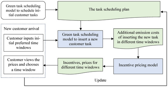
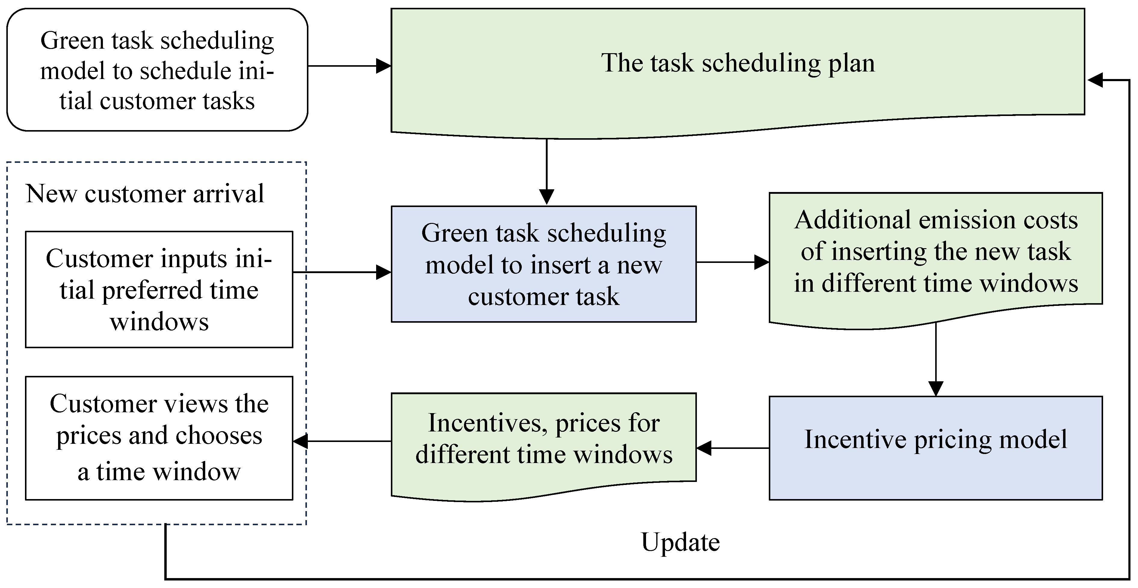
Once the customer selects a time window, the corresponding schedule from the first phase is implemented. The scheduling model is also used for the initial set of tasks, so all decisions (initial and dynamic) are supported by the same framework. Figure 1 illustrates this two-phase approach, where scheduling and pricing are integrated to help the planner dynamically update the task scheduling plan in response to incoming requests.
Figure 1.
The framework of the solution approach.
4. First Phase: The Green Vehicle Scheduling Model
The first phase model schedules or reschedules all the service tasks on hand to the vehicles with the objective to minimize the emission costs. There is a fixed number of vehicles available in the depot at the start of the planning horizon; they will all be scheduled in the day. At the start of the planning horizon, the tasks considered in the model are the initial set of customer orders, while the tasks in each of the subsequent models include the new customer orders and existing tasks that have been scheduled but have not been served yet. Each task has a required time window for service start. The time window for the new task is the assumed possible time window. The service times of different tasks can be different to represent the variations in service time.
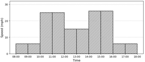
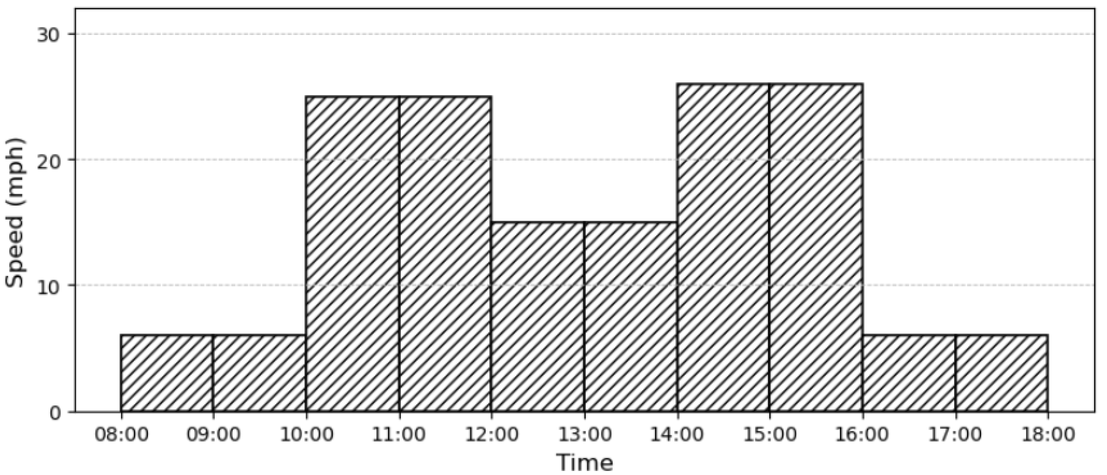
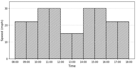
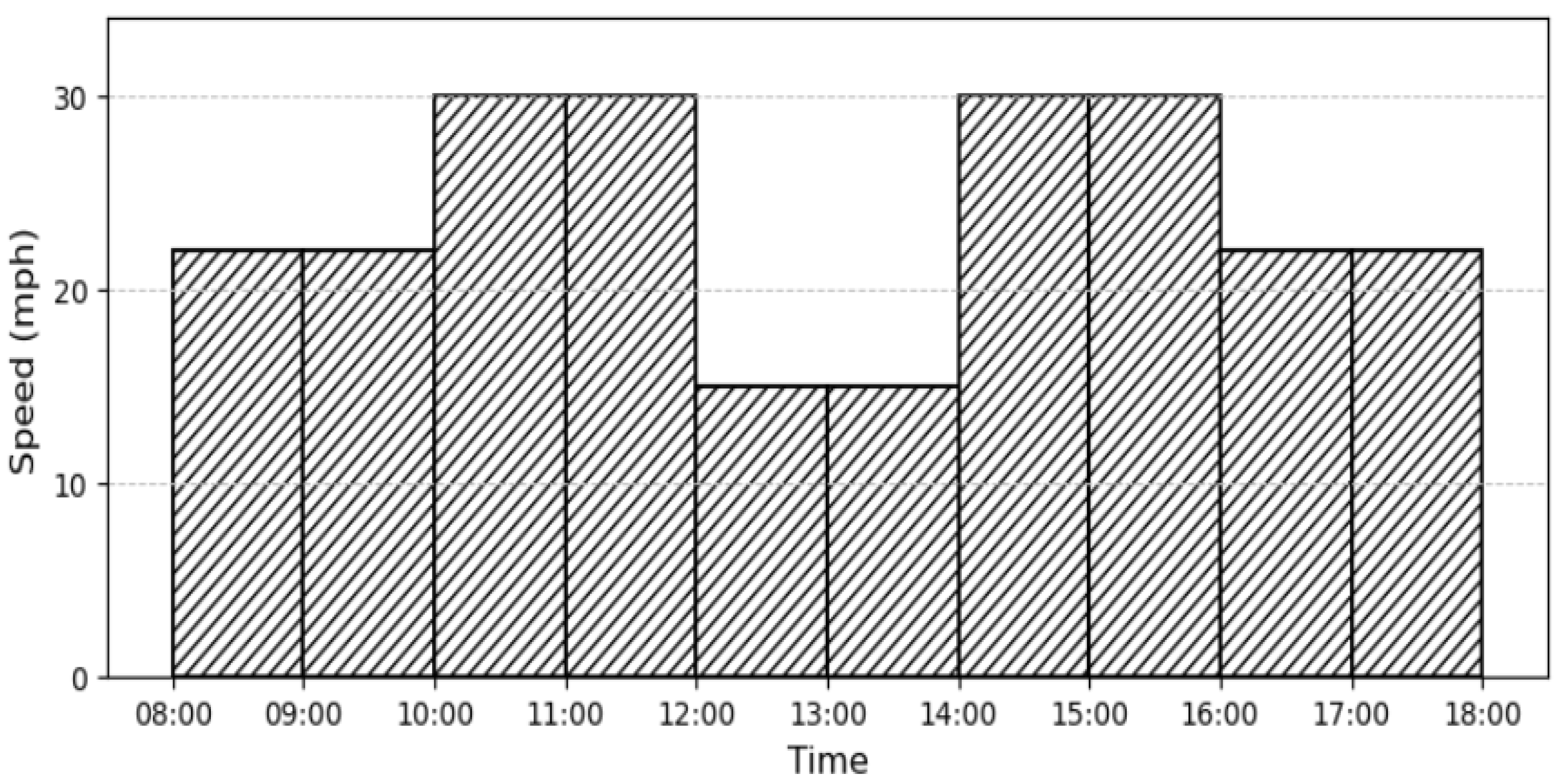
The whole planning horizon is [0, T], where T is the last time point at which a new customer can be served, where 0 indicates the earliest time after which the schedule can still be changed, and T indicates the end of a working day, correspondingly. Following Hickman et al. [41], we divide the whole planning horizon into several equal time slots. Each time slot has an average travel speed. Based on the NAEI emission model, as previously mentioned, CO2 emissions can be computed for each time slot accordingly. Figure 2 presents a speed profile over the planning horizon for London, UK, generated based on travel speed and common congestion periods summarized from Road Congestion and Travel Times reports [42]. The amounts of emissions are computed based on this profile.
Figure 2.
Speed profile over the working day for a district in London, UK.
Note that as time goes on, when a new customer order arrives, the planning horizon for the model will be shorter than the initial planning horizon. To keep the model general, we redefine the time so that the planning horizon for the model always starts at time 0 and ends at T. T will be smaller in later runs of the model. Other time-related parameters, such as time windows and time slots, will also be adjusted accordingly. At the time a new customer arrives, some existing tasks may have been started but not completed. Such tasks have to be continued without change. Until the completion time of such a task, the vehicle assigned to this task will not be available.
Notations
Parameters:
: index of customers;
: index of vehicles;
: total number of customers;
: total number of vehicles available;
: a large positive number;
: end time of the planning horizon;
: total number of time slots in the planning horizon, the length of each slot is T/n;
: beginning and ending times of the required time window in which a vehicle must arrive to customer i;
: service time needed for customer i;
: travel time between any two sites if traveling in time slot t;
: the time when vehicle j becomes available;
: emission cost for a trip in time slot t.
Variables:
: emission cost of serving customer i;
: time point when a vehicle starts traveling to customer i;
: time point at which the service to customer i starts;
;
;
;
When a new customer requests service, the scheduling problem needs to be re-solved. This is formulated as follows.
The model
Minimize
Subject to
The objective is to minimize emission costs. Constraint (1) defines the emission cost of customer i. Constraint (2) specifies that each customer is served once and by only one vehicle. Constraint (3) ensures that travel to each customer i starts in only one time slot. Constraint (4) indicates the sequence of customers served, a sub-tour elimination constraint. Constraint (5) ensures that the time window requirements of each customer must be satisfied. Constraint (6) requires that service start time must allow for travel time between customers. Constraint (7) takes effect when , which means customers i and k are both served by vehicle j, and customer i is served before customer k. Under this circumstance, the constraint ensures that the vehicle can start traveling to customer k only after it completes serving customer i. Constraints (8) and (9) identify the start and end time slot indexes. These help us to link continuous variable u and binary variable z. Constraints (10) and (11) are binary and non-negativity constraints.
5. Second Phase: The Pricing Model
When a new customer arrives with a preferred initial time window, the planner computes a price menu for each available time window. Incentives are offered for time windows that result in lower emissions, with the aim of shifting customer demand. The incentive pricing model is adapted from Campbell and Savelsbergh [33] with improvements. Their model uses a distance-based cost function, whereas the current paper applies an emission-based cost function. The emission cost of each time window is calculated using the output of the first-phase green vehicle-scheduling model. These costs are then incorporated into the pricing model to determine which windows should receive incentives and the corresponding incentive amounts.
We aim to improve upon their model in two ways. First, the number of incentives in their approach is highly restricted by the lowest initial probability of selecting a time window. Second, the time windows eligible for incentives are predetermined (see [28] for details). Our model addresses these limitations by embedding the selection of time windows into the optimization process, and by removing the restriction that ties incentive levels to the lowest initial probability.
Consistent with Campbell and Savelsbergh [33], we assume that the company has knowledge of both the likelihood of a customer choosing a particular time slot and the effect of price changes on customer behavior. With the advent of the internet, it is reasonable to assume that businesses have access to extensive historical data about their customers. For instance, online grocery shopping and delivery companies have developed booking interfaces that allow them to track purchasing behavior as well as responses to incentives and discounts.
Notations
Parameters:
h: index of time windows;
O: set of all time windows;
: probability of the current customer choosing time window h if no incentives are offered;
: additional emission cost of including the current customer into an optimized schedule (emission cost is proportional to emission);
: revenue that the current customer will bring;
: price sensitivity parameter;
B: maximum incentive that may be applied to a time window;
M2: a large positive number.
Variables:
: incentive for time window h;
z: amount of probability reduced;
: the probability that, with an incentive, time window h will be chosen by the customer;
: the probability that, without an incentive, time window h will be chosen by the customer;
;
.
The pricing model is formulated as follows.
The model
Maximize
Subject to
The objective is to maximize expected profit. The first part of the objective function represents the expected profits from the time windows that are given incentives and the second part represents the expected profits from the windows that do not receive an incentive.
Constraint (12) restricts the incentive to within the range of [0, B]. Constraints (13)–(15) calculate the adjusted probability for all h receiving incentives. If time window h does not receive an incentive, . If a time window does not receive an incentive, the probability of the customer choosing it will reduce, which is represented by constraints (16)–(20). If the adjusted probability of a time window which does not receive incentive is greater than zero, i.e., then the adjusted probability, , otherwise, . Constraint (21) ensures that the probabilities for all time windows sum to one. Constraints (22) and (23) indicate that if a time window receives an incentive, the amount of incentive is greater than zero. Constraints (24) and (25) are nonnegativity and binary constraints.
Remark 1.
Offering no incentives is a feasible solution.
When for all h, from (22), we have . Then, from the first four constraints (12) to (15), we have . Constraints (16) to (20) can be satisfied by and . Then, based on constraint (21) , we get . Since the initial probabilities satisfy , we know that z = 0. So, the solution with no incentives satisfies all the constraints, i.e., it is feasible, and the corresponding objective value is .
Remark 2.
If an incentive is offered in the optimal solution, then the solution will reduce the expected carbon dioxide emissions compared to a solution with no incentives.
Because no incentive is a feasible solution, then if , by definition, the expected revenue > . The expected revenue can be re-written as . is an additional cost in the objective function, so the expected carbon dioxide emission cost must be lower for an overall revenue increase.
In field service operations, engineers can only complete a small number of visits in a single day because each job involves time on site as well as travel. Sectors such as utilities, home appliance repair, and telecommunications typically report daily schedules of six to twelve visits per engineer. A problem size in the range of twenty to forty requests therefore reflects a normal planning horizon for a small team rather than a simplified test case. At this level, using exact optimization is entirely feasible and allows the effects of the model’s assumptions to be observed clearly. The pricing model in the second phase also remains computationally manageable. Once the choice probabilities are substituted into the revenue function, the formulation stays linear, and no nonlinear or quadratic terms arise. The number of variables grows with the number of customers and time windows, but commercial solvers handle these models quickly; in all of our tests, the pricing phase finished in well under a second. For organizations dealing with much larger daily volumes, heuristic approaches could be developed in future work, but the instance sizes used here are typical of field service environments and are well suited to exact solution methods.
To adopt this approach, a company needs to collect traffic data to develop a speed profile for their service area and incorporate this, along with the models, into a decision-support system for staff handling customer requests. Customers, on the other hand, do not need to be aware of the models or the system. When requesting service, the customer simply provides their address, the service needed and their preferred time window. The system then generates the available time windows and their corresponding prices, allowing the customer to make an informed choice.
6. Numerical Experiments
The green scheduling and pricing approach is tested using numerical experiments. The first-phase model is solved using Xpress optimizer, which applies a powerful branch-and-bound method to solve mixed integer linear programming models. The second-phase model is solved using the Lingo optimizer, which deploys both successive linear programming (SLP) and generalized reduced gradient (GRG) algorithms to solve non-linear programming models.
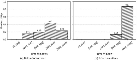
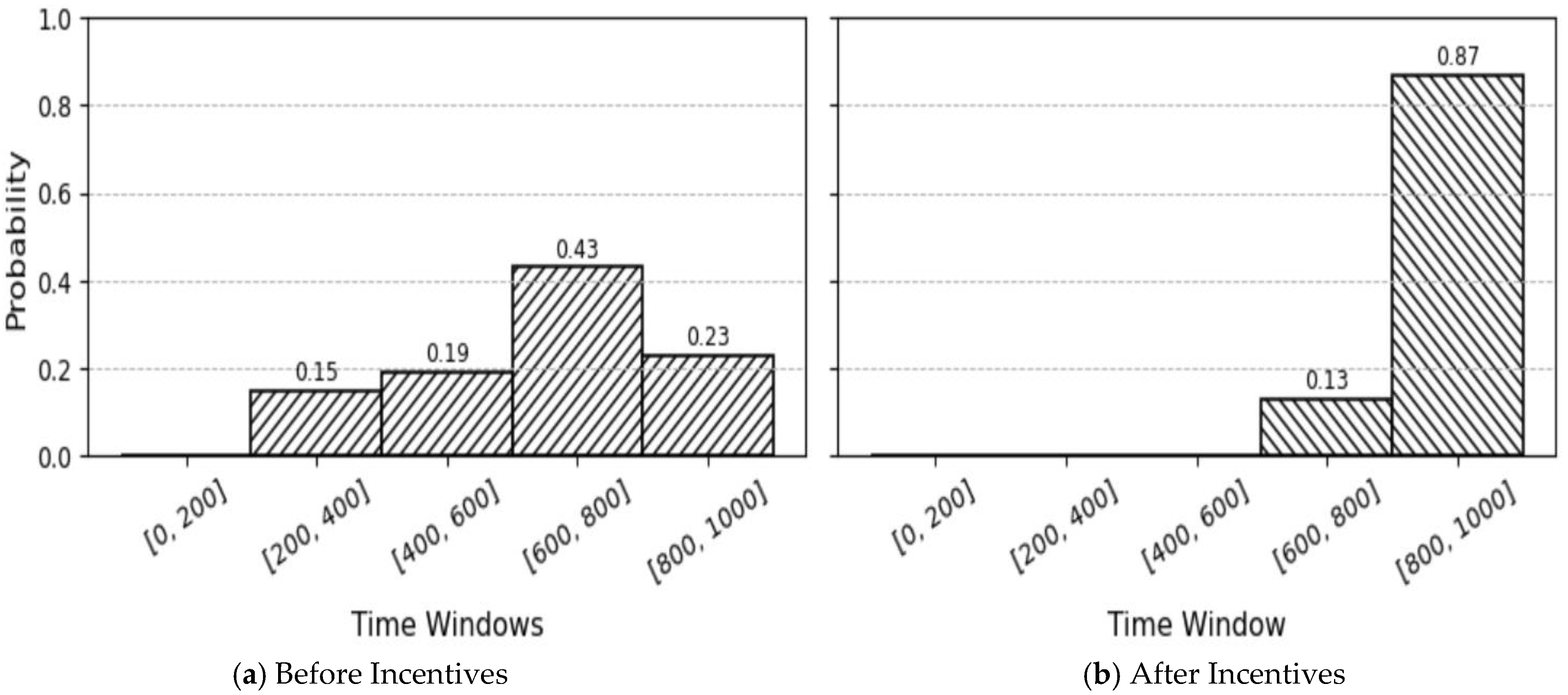
In the experiments, the planning horizon is set to one day, from 8:00 am to 6:00 pm. For convenience, we choose a time unit such that the length of this planning horizon is 1000. The whole period is divided into five equal time windows that customers may choose for their requested service to start. Reflecting the congestion conditions, the speed profile is expressed using ten time slots, as illustrated in Figure 2. The solution approach described in Section 3 is implemented by simulating customer arrivals and service operations for the whole planning horizon. The models in the first and second phases are solved using FICO Xpress Optimiser v9.7.0 and Lingo 10, respectively. We generate an initial set of customers at the beginning of the day and simulate subsequent customer arrivals using a Poisson process. For each customer arrival, a preferred time window is randomly generated. The initial probability of the customer accepting each available time window is calculated using a triangular distribution with the preferred time window as the mode. The triangular distribution is utilized because it offers several advantages for modeling customer preferences, such as being bounded and capable of accommodating varying degrees of skewness [43]. However, the pricing model does not rely on any specific distribution; users may set the ph values in the pricing model based on their own empirical data. Details of the triangular distribution are provided in Appendix A. The green scheduling model is run to obtain the emission cost of the task being scheduled in each available time window. The pricing model is then run to decide on the incentives given for each of these time windows. Table 2 shows the inputs and outputs of the pricing model for an illustrative example. The customer arrives at time 284, with an initial preference for time window [600, 800]. The initial probabilities of the customer choosing the available time windows and the emission costs for the time windows are given in Table 2. The pricing model offers incentives for time window [800, 1000], which has the lowest emission cost. The probability profiles before and after incentives can be seen in Figure 3. As can be seen from the figures in Table 2, the expected emission cost with the incentive is lower than the emission cost if the customer is scheduled in their initial preferred time window. The customer’s final choice of service time window is randomly generated using the adjusted probability profile. The task is then scheduled in the selected time window, and this customer becomes an existing customer.
Table 2.
An example customer for illustration.
Figure 3.
Customer choice probability.
6.1. Performance of Dynamic Pricing
We first compare our approach with the green scheduling method without incentives. The green scheduling method is implemented using the same simulation framework. In this method, the scheduling model in Section 4 is applied to assign each customer’s task strictly to their preferred time window.
We assume there are five vehicles available at the depot and an initial set of 10 customers at the start of the planning horizon. Customer arrivals are simulated using a Poisson process with a mean inter-arrival time of 50, resulting in approximately 20 new requests per day on average. Service times are customer-specific and randomly generated within the range [55, 150] to reflect the variations typical of such problems. Considering the time unit described earlier, with 100 units in an hour, this range is from slightly over 0.5 h to 1.5 h. While this range is based on the task durations typical of a service company we collaborated with, the approach is equally applicable to other service time ranges.
We generate 10 sets of customer arrival times, initial preferred time windows, and service times, each representing one day. Each dataset is referred to as a scenario. Since each customer’s final choice is uncertain, results may vary across different runs even within the same scenario. To account for this, we run each of the 10 scenarios 10 times and compute the average emissions and profit.
We assume that each customer generates a revenue of 30, which is approximately 10 times the emission cost, as additional expenses (e.g., engineer wages) must also be covered to ensure profitability. Profit is calculated as revenue minus incentives and emission costs. We then compare the two methods in terms of CO2 emission cost and profit. The results are reported in Table 3 and Table 4, respectively.
Table 3.
Comparing CO2 emissions.
Table 4.
Comparing profits.
The results presented in Table 3 and Table 4 clearly demonstrate the effects of incentives on both the emission cost and the profit generated. Our incentive model reduces the CO2 emission cost by 10.80% on average, compared to a green vehicle scheduling method without an incentive. Meanwhile, the average profit increases by 1.65%. The average results show that the incentive pricing model can both increase profits and reduce carbon dioxide emissions significantly. All experiments were run on a 64-bit Windows PC with an Intel i5 quad-core processor and 8 GB RAM, using Xpress Optimiser for the MILP scheduling phase and LINGO for the pricing phase. For approximately 30 customers per day with five time windows, the total CPU time for 10 replications of a scenario was approximately 20 s on average, with the pricing phase taking negligible time relative to scheduling.
6.2. Sensitivity of the Two-Phase Model
6.2.1. The Ratio of Existing Customers
The average percentage of existing customers is about 33% in the initial setting (10 from a total of 30 on average). We change the ratio of existing customers in the system, but use the same setup for other parameters as in the first experiment. We increase the average percentage of existing customers to about 50% (15 out of 30) and then to about 67% (20 out of 30). The number of new customers arriving will now be 15 and 10, respectively. We examine how the number of existing customers in the system affects the emission savings and profit. The emission cost and profit results are shown in Table 5 and Table 6, respectively. For the ratios of 53% and 67% existing customers, the average savings in emission costs become 5.77% and 3.37%, respectively, and the average profit improvements become 0.82% and 0.36%, respectively. These results demonstrate that as the percentage of existing customers increases, there are fewer new customers arriving during the day, and so the system becomes less dynamic. The use of the pricing techniques is restricted. Therefore, there is less room for saving on CO2 emission costs and for profit improvement.
Table 5.
Comparing emissions and profit with around 50% existing customers.
Table 6.
Comparing emissions and profit with around 67% existing customers.
6.2.2. Variation in Emission Level over Congested/Non-Congested Period
We test the performance of our pricing model in a situation where there is less variation in emission cost for different time slots. For example, there is less congestion and the travel speed varies less during the day in areas such as Yorkshire and the Humber, UK. The less variable speed profile of a day in Yorkshire and the Humber, UK is obtained as shown in Figure 4.
Figure 4.
Speed profile, with lower variation, for Yorkshire and the Humber, UK.
Assuming this new speed profile, we test our model using the same 10 scenarios as in Table 3 and Table 4, and each scenario is run 10 times. The results for emission cost and profit are shown in Table 7. With the new speed profile, our model only saves 0.23% in CO2 costs. The profit improvement also becomes only 0.02%. As the emission levels vary less across the day, the differences between the costs of different time slots are much smaller. Thus, the attempt to use incentives to shift customers’ demand makes less difference. Hence, the speed profile plays a central role to the effectiveness of this pricing model.
Table 7.
Results for a speed profile with lower variation.
6.2.3. Patterns of Customer Arrivals
We further test the effect of customer arrival patterns on the performance of our model. We run 10 scenarios that have the same existing customers as the first 10 scenarios in the first experiment, but subsequent customers arrive in three different patterns. In each pattern, the total number of customers is the same, 30. This means that the average number of newly arriving customers is 20 for each pattern. For pattern 1, the average number of customers arriving in the first and second halves of the planning horizon are 10 and 10, respectively. For pattern 2, the average number of customers arriving in the first and second halves of the planning horizon are 5 and 15, respectively, and for pattern 3, they are 15 and 5, respectively. Compared to pattern 1, where customers arrive more evenly across the planning horizon, pattern 3 provides the planner with more opportunity to price dynamically and influence the customer’s choices, while pattern 2 provides less opportunity. The savings in the emission costs and the profit improvement for the three arrival patterns are shown in Table 8.
Table 8.
Results for different patterns of customer arrival.
The experimental results show that when more customers arrive in the system early, more savings in CO2 emission costs and a greater improvement in profit are expected. Over time we would expect strategic customers to learn that earlier arrival into the system results in them receiving the service for a lower price. This may shift the customer arrival patterns over time to the more profitable one.
6.3. Further Experiments and Discussions
To test the scalability of the approach, further experiments were carried out on instances where the fleet size was doubled to 10 vehicles. Other settings, including the planning horizon, speed profile, and time/cost parameters, remained consistent with the base case described earlier. The number of existing customers also doubled to 20. To stretch the system’s limits, the rate of new customer arrivals was set slightly higher than double that of the 5-vehicle case. Additionally, these scenarios were tested using different values for the price sensitivity parameter, β. Again, 10 instances were generated, and 10 repetitions were run for each scenario. As more customers arrive, the system can reject a customer if there is no suitable time window to accommodate them. As a result, the number of customers served in the same instance may vary with different β and across different runs. The overall average results are presented in Table 9.
Table 9.
Average results with different price sensitivity parameters for larger problem instances.
Results for the larger fleet and higher arrival rates mirror those observed in previous sections. The phase-two pricing model successfully leverages phase-one emission data to guide customers toward greener time windows, yielding significant emission reductions and profit gains. Notably, these benefits are more substantial under a high workload than in the baseline 5-vehicle case. The incentive structure also improves resource utilization by increasing the number of customers served. Since higher throughput inevitably increases absolute emissions, we use emission cost per customer as a normalized measure to ensure a fair comparison.
Comparing the results across different price sensitivity values, Table 9 shows that as β increases at lower levels (from 0 to 0.05 and then to 0.10), the number of customers served, the emission cost per customer and the total profit all show marked improvements. However, once β reaches a certain threshold, the improvements in customers served and in per-customer emission cost tend to stabilize. In contrast, total profit continues to increase. This is because, as customers become more price-sensitive, fewer incentives are required to shift their demand toward low-emission windows, which produces a greater profit increase, given the stabilized revenue and emission costs.
As indicated by the results, although emission costs represent only approximately 10% of total revenue, the cost differentiation between various time slots plays a critical role in influencing customer choices. To illustrate this more clearly, we conducted an additional experiment using the same instances but excluding emission costs from the pricing model. In this setup, the first-phase model maximizes the revenue from scheduling the customer into each time window. By ignoring emission cost, the model effectively reduces to evaluating the feasibility of each time window: revenue is set to 30 if feasible and 0 otherwise. The second-phase pricing model (with β = 0.1) then maximizes profit, defined here as revenue minus the costs of incentives.
These results are presented in the final row of Table 10. The first two rows are included for comparison. They correspond to specific scenarios from Table 9: the first row represents a baseline green scheduling scenario without incentives (β = 0), and the second row reflects the integrated model, considering both emission costs and incentives (β = 0.1). When emission costs are excluded, the pricing model identifies feasible time windows but lacks a clear optimization objective for selection, thereby limiting the extent to which incentives can shift customer behavior to maximize profit. Consequently, the total incentive amount utilized is lower compared to the integrated case, and so is the number of customers served. Furthermore, because emissions are not explicitly optimized, the resulting schedule incurs higher emission costs and lower total profit, though the profit per customer is slightly higher (25.87 vs. 25.70. Nevertheless, the results demonstrate that pricing remains effective, as performance still exceeds that of the no-incentives scenario.
Table 10.
Average results with different first-phase objectives for larger problem instances.
For the larger instances in this subsection, the computation time of the models remains short. Upon a customer’s arrival, the system needs less than one second to determine the service prices for the available time windows. These exact models are, therefore, highly effective for fleets of up to 10 vehicles. However, tests on instances with 15 vehicles revealed that while computation time is generally short, the first-phase model occasionally takes significantly longer to solve. This performance variability demonstrates the necessity of heuristic solutions for the first-phase model when managing fleet sizes larger than in the experiment instances here.
7. GenAI Interpretation and Decision Insights
In Section 6, we have shown that the two-phase framework for green scheduling and dynamic pricing produces strong operational results. To turn this framework into a practical decision-support system that provides actionable insights for planners, customers, and management, we incorporate a GenAI interpretation assistant. Prior research that has used GenAI as an innovative tool includes Ebert et al. [44], who used it to enhance software engineering productivity, and Iatrellis et al. [45], who showed that generative AI models (e.g., GANs, VAEs, transformers) can improve consumer behavior prediction using large/unstructured data for personalization, inventory management, and customer retention. Madanchian et al. [46] demonstrated that AI-driven recommendations can improve academic advising to better support students and make advising practices more effective and sustainable. In our approach, the GenAI component is used as an interpretation layer that converts the optimization outputs into human-readable explanations and decision-support narratives. The schedules and incentives decisions proposed by the two-phase mathematical models in Section 6 are input into the GenAI model, which is prompted to translate those outputs into concise summaries, explanations of incentives and emissions, and action recommendations. Because the LLM is used as an offline interpretation tool, we did not train it on a bespoke dataset. Instead, we evaluated it on optimization instances generated in our experiments and compared its interpretations against human-written references. This section illustrates the added value by demonstrating the types of insights it can extract from the results in Section 6.
From the results tables in Section 6, GenAI can quickly identify which time windows have high or low emissions, how arrival patterns affect system performance, when incentives increase profit and when they do not, where scheduling bottlenecks or slack occur, regional differences in congestion sensitivity, the maximum and minimum improvements the system can achieve, and the most effective strategies for shifting customers. A few examples of its effectiveness are provided below.
One of the most important insights concerns how incentives influence customer behavior, specifically the shift in demand between high- and low-emission time windows. Across the ten scenarios in the baseline experiment, the model achieves an average CO2 reduction of 10.80%. When these results are provided to a GenAI tool (e.g., ChatGPT 5.1), it can identify where further improvements could be made to shift customer behavior. For example, an AI insight reads, “Mid-day windows consistently generate the highest marginal emissions; strengthening the guidance mechanisms during these hours—whether through pricing, information cues, or green labelling—will help shift customers into cleaner, lower-congestion windows”.
A second insight relates to the timing of customer arrivals. The results show that earlier arrival patterns allow the model to achieve emission reductions of up to 17.26%, compared with only 5.26% when most customers arrive later in the day. An AI interpretation reads, “Early arrivals increase rescheduling flexibility; features such as early booking discounts or interface nudges will maximise CO2 savings”. GenAI can also improve managerial understanding of how incentives contribute to profitability. For example,
“As shown in Table 4, profit increases by an average of 1.65% across the ten scenarios, and reaches 5.19% in Scenario 4, where incentives most effectively shift customers away from highly congested, high-emission windows. This scenario is characterized by particularly high baseline emissions—146.71 units in Table 3—which explains why the incentive-based strategy yields a strong financial return. The GenAI interpretation captures this pattern, for example: “When baseline emissions exceed 120 units, incentives create net financial gain by avoiding high-emission insertions.” This helps planners identify when incentives are likely to generate a positive financial return and when they may not.”
Finally, GenAI can detect conditions in which incentives are unlikely to be effective. For example, an AI insight reads, “Under the low-variation congestion profile used for the Yorkshire and Humber region, emission savings fall to 0.23%, and profit improvement to only 0.02%”, and “In low-variation speed profiles, incentive-based scheduling becomes ineffective; consider restructuring time windows or introducing low-emission vehicles instead”. Incorporating GenAI enhances the interpretation of the two-phase optimisation system and turns it into a practical decision-support tool for managers, particularly when decisions must be made in real time to improve both environmental performance and operational profitability.
We validate that the GenAI interpretation is consistent with human decision-making. We performed an expert cross-check using representative optimization outputs from the experiments in Section 6 (baseline scenarios and sensitivity cases). Two experts reviewed the optimization results (objective values, emissions, and profit changes, and scenario comparisons) and produced interpretations and recommended actions (e.g., which time windows should be incentivized and why). We then compared these with the GenAI interpretations produced from the same optimization outputs. In all tested cases, the GenAI summaries were consistent with the experts’ qualitative conclusions (direction of change, identification of high/low emission windows, and rationale for incentives), and all numerical statements reported in the GenAI text were verified against the optimization results. This provides evidence that the GenAI component supports human decision-making by communicating the optimization outcomes more clearly and provides sensible recommendations.
8. Conclusions
In this paper, we have studied a problem where a company sends engineers with vehicles to customer sites to provide services. Throughout the day, customers call or visit a website requesting services with preferred time windows, and for each customer, the company needs to schedule the service task to a vehicle. We proposed a new two-phase approach to this problem. The first phase solves vehicle-scheduling models with the objective of minimizing CO2 emissions, and the second phase solves a dynamic pricing model to maximize profit. The approach was tested through computational experiments. The results showed a significant reduction in the amount of CO2 emissions as well as a significant improvement in the total profits for test cases in London, UK. We also carried out sensitivity tests, in which the results showed that when the system is less dynamic, i.e., fewer new incoming customers, or lower emission variation, the reduction in CO2 emissions and profit improvement are lower. The patterns of customer arrival also affect the results. Although our models were developed under certain assumptions, they are applicable to some real-life situations. The new approach is an attempt in a new direction of research exploring the combination of Green VRP and dynamic pricing techniques. An additional contribution of this study is the inclusion of a GenAI interpretation module, which supports decision makers by explaining optimization outputs and helping them use the system in real time. The study offers insight into how factors such as emission variability, the timing of customer arrivals, and the level of system dynamism influence both emissions and profit. The added complexity discussion helps to clarify what makes each phase of the model challenging and why the two-stage structure is appropriate. The decision-support contribution is further strengthened by the GenAI interpretation component, which helps planners make practical use of the model’s outputs in real time.
This study considered the problem of a confined service area where routing differences are minor, and hence, it could focus on time-dependent congestion effects; the model is not generalizable for more spatially dispersed settings. Furthermore, our optimization approach was tested on problems of limited scale, aligned with the setting of our partnered service company; however, substantially larger instances may become computationally demanding and would require metaheuristic methods to obtain good solutions within practical time limits.
Future work could incorporate a learning component that evaluates how planners respond to GenAI recommendations and that updates its decisions over time, allowing the system to adapt its guidance based on observed effectiveness. The model could also incorporate heterogeneous fleets, variable service durations, and real-time traffic updates to improve the accuracy and robustness of emissions estimates. In addition, fast heuristic methods for the phase-one scheduling model could be developed to support larger problem instances.
Author Contributions
Conceptualization, Y.Z., R.M. and J.L.; methodology, Y.Z., J.L., R.M. and C.B.; formal analysis, Y.Z. and J.L.; writing—original draft, Y.Z. and R.M.; writing—review and editing, J.L. and C.B.; supervision, R.M. and J.L. All authors have read and agreed to the published version of the manuscript.
Funding
This research received no external funding.
Institutional Review Board Statement
Not applicable.
Informed Consent Statement
Not applicable.
Data Availability Statement
The original contributions presented in this study are included in the article. Further inquiries can be directed to the corresponding author.
Conflicts of Interest
Author Yizi Zhou was employed by the Huawei Technologies Co., Ltd., Bantian Huawei Base. The remaining authors declare that the research was conducted in the absence of any commercial or financial relationships that could be construed as a potential conflict of interest.
Appendix A
Triangular Method for Calculating Initial Probabilities
For each customer, the probability that this customer will choose each available time window is calculated using a triangular distribution. The company is a monopoly, and therefore, the probability that a customer walks away without purchasing the service is zero. The probabilities of the customer choosing their preferred time window or the other time windows are calculated based on a triangular distribution:
tmin: customer arrival time window or earliest time window available, whichever is earlier.
x: any of the available time windows; x = tmin, …, 5.
d: customer’s initial preferred time window.
The probabilities of each available time window are as follows:
References
- UK Government, Department for Transport. Greenhouse Gas Emissions from Transport in 2023. 2023. Available online: https://www.gov.uk/government/statistics/transport-and-environment-statistics-2023--2/greenhouse-gas-emissions-from-transport-in-2023 (accessed on 16 September 2025).
- UK Government, Department for Energy Security and Net Zero. 2024 Provisional Greenhouse Gas Emissions: Statistical Release. 2025. Available online: https://assets.publishing.service.gov.uk/media/67e4060df356a2dc0e39b4cd/2024-provisional-greenhouse-gas-emissions-statistics-statistical-release.pdf (accessed on 16 September 2025).
- Spherical Insights & Consulting. United Kingdom Home Services Market Report 2024–2035. 2025. Available online: https://www.sphericalinsights.com/reports/united-kingdom-home-services-market (accessed on 16 September 2025).
- Expert Market Research. United Kingdom Field Service Management Market Report and Forecast 2025–2034. 2025. Available online: https://www.expertmarketresearch.com/reports/uk-field-service-management-market (accessed on 16 September 2025).
- Climate Change Committee (CCC). The Seventh Carbon Budget; Climate Change Committee: London, UK, 2025. Available online: https://www.theccc.org.uk/publication/the-seventh-carbon-budget/ (accessed on 16 September 2025).
- Li, H.; Zhou, J.; Xu, K. Evolution of green vehicle routing problem: A bibliometric and visualized review. Sustainability 2023, 15, 16149. [Google Scholar] [CrossRef] [Scilit]
- Garside, A.K.; Ahmad, R.; Muhtazaruddin, M.N.B. A recent review of solution approaches for green vehicle routing problem and its variants. Oper. Res. Perspect. 2024, 12, 100303. [Google Scholar] [CrossRef] [Scilit]
- Wang, Y.; Duan, J.; Sun, J.; Zhang, Q.; Ye, T. A green vehicle routing problem with time-varying speeds and joint distribution. Sustainability 2025, 17, 7515. [Google Scholar] [CrossRef] [Scilit]
- Apaydin, O.; Gonullu, M.T. Emission control with route optimization in solid waste collection process: A case study. Sadhana 2008, 33, 71–82. [Google Scholar] [CrossRef] [Scilit]
- Ubeda, S.; Arcelus, F.J.; Faulin, J. Green logistics at Eroski: A case study. Int. J. Prod. Econ. 2011, 131, 44–51. [Google Scholar] [CrossRef] [Scilit]
- Eglese, R.; Black, D. Optimizing the routing of vehicles. In Green Logistics: Improving the Environmental Sustainability of Logistics; McKinnon, A., Cullinane, S., Browne, M., Whiteing, A., Eds.; Kogan Page: London, UK, 2010; pp. 215–228. [Google Scholar]
- Figliozzi, M. Vehicle routing problem for emissions minimization. Transp. Res. Rec. J. Transp. Res. Board 2010, 2197, 1–7. [Google Scholar] [CrossRef] [Scilit]
- Jabali, O.; Woensel, T.; de Kok, A.G. Analysis of travel times and CO2 emissions in time-dependent vehicle routing. Prod. Oper. Manag. 2012, 21, 1060–1074. [Google Scholar] [CrossRef] [Scilit]
- Maden, W.; Eglese, R.; Black, D. Vehicle routing and scheduling with time-varying data: A case study. J. Oper. Res. Soc. 2010, 61, 515–522. [Google Scholar] [CrossRef] [Scilit]
- Turkensteen, M. The accuracy of carbon emission and fuel consumption computations in green vehicle routing. Eur. J. Oper. Res. 2017, 262, 647–659. [Google Scholar] [CrossRef] [Scilit]
- Demir, E.; Bektaş, T.; Laporte, G. A review of recent research on green road freight transportation. Eur. J. Oper. Res. 2014, 237, 775–793. [Google Scholar] [CrossRef] [Scilit]
- Ooi, K.B.; Tan, G.W.H.; Al-Emran, M.; Al-Sharafi, M.A.; Capatina, A.; Chakraborty, A.; Dwivedi, Y.K.; Huang, T.-L.; Kar, A.K.; Lee, V.-H.; et al. The potential of generative artificial intelligence across disciplines: Perspectives and future directions. J. Comput. Inf. Syst. 2025, 65, 76–107. [Google Scholar] [CrossRef] [Scilit]
- Khlie, K.; Benmamoun, Z.; Jebbor, I.; Hachimi, H. Comparison of Generative AI Models in Supply Chain Management: Benefits, Applications and Challenges. In Proceedings of the 2024 10th International Conference on Optimization and Applications (ICOA), Almeria, Spain, 17–18 October 2024; pp. 1–7. [Google Scholar] [CrossRef] [Scilit]
- Jebbor, I.; Benmamoun, Z.; Hachimi, H. Leveraging Digital Twins and Metaverse Technologies for Sustainable Circular Operations: A Comprehensive Literature Review. Circ. Econ. Sust. 2025, 5, 5795–5848. [Google Scholar] [CrossRef] [Scilit]
- Voß, S. Successfully using ChatGPT in logistics: Are we there yet? In Proceedings of the International Conference on Computational Logistics, Berlin, Germany, 6–8 September 2023; Springer Nature: Cham, Switzerland, 2023; pp. 3–17. [Google Scholar]
- Sun, R.; Yu, G.; Chen, P.; Li, B. Artificial Intelligence-driven Optimization Methods for Vehicle Scheduling and Dispatching: An Overview and Further Directions. IEEE Veh. Technol. Mag. 2026, 2–11. [Google Scholar] [CrossRef] [Scilit]
- Yang, C.; Wang, X.; Lu, Y.; Liu, H.; Le, Q.V.; Zhou, D.; Chen, X. Large language models as optimizers. In Proceedings of the Twelfth International Conference on Learning Representations, Vienna, Austria, 7–11 May 2024. [Google Scholar]
- Zafar, U.; Bayhan, S. Using large language models to solve the electric vehicle routing problem with advanced prompting techniques. In Proceedings of the 2025 IEEE 19th International Conference on Compatibility, Power Electronics and Power Engineering (CPE-POWERENG), Antalya, Türkiye, 20–22 May 2025; IEEE: New York, NY, USA, 2025; pp. 1–6. [Google Scholar]
- Chi, M.; Pang, W.; Wu, X.; Zhao, P.; Li, Y.; Wang, T.; Qian, J.; Xiao, Y.; Wang, L.; Zhou, Y. A generalized neural solver based on LLM-guided heuristic evoluation framework for solving diverse variants of vehicle routing problems. Expert Syst. Appl. 2026, 296, 128876. [Google Scholar] [CrossRef] [Scilit]
- Chen, R.; Song, W.; Zu, W.; Dong, Z.; Guo, Z.; Sun, F.; Tian, Z.; Wang, J. An LLM-driven framework for multiple-vehicle dispatching and navigation in smart city landscapes. In Proceedings of the 2024 IEEE International Conference on Robotics and Automation (ICRA), Yokohama, Japan, 13–17 May 2024; IEEE: New York, NY, USA, 2024; pp. 2147–2153. [Google Scholar]
- Huang, Y.; Zhang, W.; Feng, L.; Wu, X.; Tan, K.C. How multimodal integration boost the performance of llm for optimization: Case study on capacitated vehicle routing problems. In Proceedings of the 2025 IEEE Symposium for Multidisciplinary Computational Intelligence Incubators (MCII), Trondheim, Norway, 17–20 March 2025; IEEE: New York, NY, USA, 2025; pp. 1–7. [Google Scholar]
- Rothstein, M. An airline overbooking model. Transp. Sci. 1971, 5, 180–192. [Google Scholar] [CrossRef] [Scilit]
- Littlewood, K. Special issue papers: Forecasting and control of passenger bookings. J. Revenue Pricing Manag. 2005, 4, 111–123. [Google Scholar] [CrossRef] [Scilit]
- Elmaghraby, W.; Keskinocak, P. Dynamic pricing in the presence of inventory considerations: Research overview, current practices, and future directions. Manag. Sci. 2003, 49, 1287–1309. [Google Scholar] [CrossRef] [Scilit]
- Strauss, A.; Gulpinar, N.; Zheng, Y. Dynamic pricing of flexible time slots for attended home delivery. Eur. J. Oper. Res. 2020, 294, 1022–1041. [Google Scholar] [CrossRef] [Scilit]
- Yang, X.; Strauss, A.K.; Currie, C.S.; Eglese, R. Choice-based demand management and vehicle routing in e-fulfilment. Transp. Sci. 2014, 50, 473–488. [Google Scholar] [CrossRef] [Scilit]
- Cleophas, C.; Ehmke, J.F. When are deliveries profitable? Bus. Inf. Syst. Eng. 2014, 6, 153–163. [Google Scholar] [CrossRef] [Scilit]
- Campbell, A.M.; Savelsbergh, M. Incentive schemes for attended home delivery services. Transp. Sci. 2006, 40, 327–341. [Google Scholar] [CrossRef] [Scilit]
- Klein, R.; Koch, S.; Steinhardt, C.; Strauss, A.K. A review of revenue management: Recent generalizations and advances in industry applications. Eur. J. Oper. Res. 2019, 284, 397–412. [Google Scholar] [CrossRef] [Scilit]
- Strauss, A.K.; Klein, R.; Steinhardt, C. A review of choice-based revenue management: Theory and methods. Eur. J. Oper. Res. 2018, 271, 375–387. [Google Scholar] [CrossRef] [Scilit]
- Çimen, M.; Soysal, M. Time-dependent green vehicle routing problem with stochastic vehicle speeds: An approximate dynamic programming algorithm. Transp. Res. D Transp. Environ. 2017, 54, 82–98. [Google Scholar] [CrossRef] [Scilit]
- Bai, Q.; Yin, X.; Lim, M.K.; Dong, C. Low-carbon VRP for cold chain logistics considering real-time traffic conditions in the road network. Ind. Manag. Data Syst. 2022, 122, 521–543. [Google Scholar] [CrossRef] [Scilit]
- Zhou, Y.; Mandania, R.; Liu, J. Green vehicle routing and dynamic pricing for scheduling on-site services. Int. J. Prod. Econ. 2022, 254, 108602. [Google Scholar] [CrossRef] [Scilit]
- Liu, Y.; Baldacci, R.; Zhou, J.; Yu, Y.; Zhang, Y.; Sun, W. Efficient feasibility checks and an adaptive large neighborhood search algorithm for the time-dependent green vehicle routing problem with time windows. Eur. J. Oper. Res. 2023, 310, 133–155. [Google Scholar] [CrossRef] [Scilit]
- Kervola, H.; Kallionpää, E.; Liimatainen, H. Delivering goods using a baby pram: The sustainability of last-mile logistics business models. Sustainability 2022, 14, 14031. [Google Scholar] [CrossRef] [Scilit]
- Hickman, J.; Hassel, D.; Joumard, R.; Samaras, Z.; Sorenson, S. Methodology for Calculating Transport Emissions and Energy Consumption; European Commission: Luxembourg, 1999; ISBN 92-828-6785-4. [Google Scholar]
- Department for Transport. Road Congestion and Travel Times Collection. 2025. Available online: https://www.gov.uk/government/collections/road-congestion-and-reliability-statistics (accessed on 8 March 2026).
- Dekker, T. Asymmetric triangular mixing densities for mixed logit models. J. Choice Model. 2016, 21, 48–55. [Google Scholar] [CrossRef] [Scilit]
- Ebert, C.; Louridas, P.; Ebert, C. Generative AI for Software Practitioners. IEEE Softw. 2023, 40, 30–38. [Google Scholar] [CrossRef] [Scilit]
- Madanchian, M. Generative AI for Consumer Behavior Prediction: Techniques and Applications. Sustainability 2024, 16, 9963. [Google Scholar] [CrossRef] [Scilit]
- Iatrellis, O.; Samaras, N.; Kokkinos, K.; Panagiotakopoulos, T. Leveraging Generative AI for Sustainable Academic Advising: Enhancing Educational Practices through AI-Driven Recommendations. Sustainability 2024, 16, 7829. [Google Scholar] [CrossRef] [Scilit]

Disclaimer/Publisher’s Note: The statements, opinions and data contained in all publications are solely those of the individual author(s) and contributor(s) and not of MDPI and/or the editor(s). MDPI and/or the editor(s) disclaim responsibility for any injury to people or property resulting from any ideas, methods, instructions or products referred to in the content. |
© 2026 by the authors. Licensee MDPI, Basel, Switzerland. This article is an open access article distributed under the terms and conditions of the Creative Commons Attribution (CC BY) license.