


Abstract
Control measures for pine wilt disease (PWD) are widely implemented, yet multi-year field comparisons that track biodiversity trajectories across contrasting management regimes remain limited. We conducted a 3-year (2023–2025) replicated study across nine pine-forest sites in Gyeongsangnam-do, Republic of Korea, comparing three management regimes (Clear-cut, Fumigation/Aerial, Unmanaged) to evaluate regime-associated patterns in ground-active beetle diversity, activity density, and community composition while considering understory vegetation cover. Regime-associated differences were consistent but dynamic: Unmanaged stands generally supported higher richness and Shannon diversity (H′), Clear-cut stands showed the lowest diversity immediately after harvest, and Fumigation/Aerial stands maintained the highest activity density. Assemblage composition separated strongly among regimes within each year, and indicator taxa highlighted regime-associated assemblage states, notably Pheropsophus jessoensis (Fumigation/Aerial), Carabus tuberculosus (Clear-cut), and Blindus strigosus (Unmanaged). Because regimes were assigned at the site level and were partially confounded by geographic region, we interpreted these outcomes as region-structured, regime-associated patterns rather than strictly causal effects. We recommend integrating PWD management with retention forestry (e.g., partial canopy and deadwood retention) and routine biodiversity monitoring to reconcile effective disease suppression with the long-term conservation of forest biodiversity.
1. Introduction
Pine wilt disease (PWD), a lethal condition caused by the nematode Bursaphelenchus xylophilus and transmitted by the longhorn beetle (Monochamus spp.; Coleoptera: Cerambycidae), poses a persistent threat to coniferous forests across East Asia and other regions [1,2]. The rapid induction of tree mortality by the disease simplifies stand structure and causes substantial economic losses [1]. In response, countries such as the Republic of Korea have implemented a range of interventions, including sanitation felling and clear-cutting operations to remove infection sources, the fumigation of logs, and seasonal aerial insecticide applications targeting vector populations [3,4,5,6,7]. Although necessary for suppression, these actions can significantly alter physical structure, microclimate, and resource availability, with potential unintended consequences for non-target biodiversity [5,7,8,9,10]. Therefore, formulating sustainable forest health policies requires evidence that jointly evaluates disease control efficacy and the associated ecological costs.
Ground beetles and associated assemblages (Coleoptera) serve as effective bioindicators of forest habitat quality and management impacts [11,12,13]. Their utility stems from their diverse functional roles (e.g., predatory, saproxylic, phytophagous, and detritivorous) and rapid responses to changes in microhabitat structure. A robust body of research has confirmed that logging history and deadwood availability—especially coarse woody debris (CWD), as well as stumps and stump-handling practices (e.g., stump retention vs. removal through extraction, and mechanical stump milling/soil preparation)—are primary drivers of beetle diversity [10,14,15]. For example, Staněk et al. reported that clearings without mechanical soil preparation (i.e., without stump milling) supported higher richness of epigeic arthropods than mechanically prepared clearings, underscoring the biodiversity relevance of stumps and stump-handling practices [15]. In the Korean context, these ground-active assemblages are taxonomically well-documented and frequently surveyed in pine forests, providing a practical lens to assess the ecological side effects of PWD control [16,17,18].
Despite widespread PWD control efforts, rigorous multi-year comparisons of alternative control portfolios remain scarce, particularly studies that explicitly test regime × year interactions while accounting for habitat covariates. This is an important knowledge gap. To design control strategies that effectively reduce disease spread while safeguarding biodiversity, we must separate short-term fluctuations from persistent assemblage shifts and quantify the mediating role of habitat structures such as understory vegetation.
To address this gap, we assembled a 3-year (2023–2025) multi-site dataset from southern Korea spanning three PWD management regimes: (i) clear-cutting (including sanitation felling) (hereafter Clear-cut), (ii) fumigation with seasonal aerial insecticide control (hereafter Fumigation/Aerial), and (iii) unmanaged stands (hereafter Unmanaged). We implemented standardized passive and active sampling across replicated sites within each regime and measured understory vegetation cover as a plot-level covariate. This design enabled the evaluation of regime-associated differences in both alpha diversity (species richness, Shannon index H′, total abundance) and beta diversity (compositional dissimilarity), as well as the effect of habitat structure on these management outcomes.
Specifically, we posed the following questions: • Q1 (alpha diversity): Do species richness, H′, and total abundance differ among control regimes, and do these differences remain consistent across years? • Q2 (beta diversity): Do assemblage compositions separate clearly among regimes in multivariate space (based on Bray–Curtis dissimilarity), as tested using permutational multivariate analysis of variance (PERMANOVA) [19,20,21]? • Q3 (environmental mediation): How much of the variation in alpha and beta diversity can be explained by understory vegetation cover relative to the direct effects of management regimes [11,13,14]?
Based on previous studies on logging intensity [11,13,14], we hypothesized the following: (H1) Clear-cut stands would initially show the lowest richness and H′ owing to structural simplification and microclimatic extremes, followed by partial recovery as vegetation regrows. (H2) Fumigation/Aerial stands, while retaining an overstory structure, may exhibit intermediate diversity if sensitive non-target taxa decline following chemical control [5,6,7]. (H3) Unmanaged stands would display higher evenness and greater contributions from predator and saprophage guilds, supported by more complex vertical structures and deadwood resources [11,13,14]. (H4) The assemblage composition is significantly different among all regimes. (H5) Understory vegetation cover would act as a significant covariate mediating diversity responses [10,11,12].
By integrating a replicated, multi-year, multi-regime design with an explicit habitat covariate, our study provides an operational baseline for evidence-based, ecologically informed PWD management. It quantifies how common control strategies influence beetle communities in Korean pine forests and identifies conditions in which biodiversity costs can be minimized.
2. Materials and Methods
2.1. Study Area and Regimes
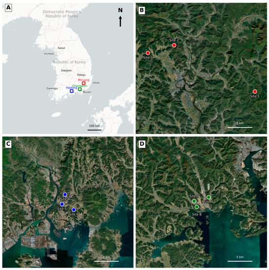
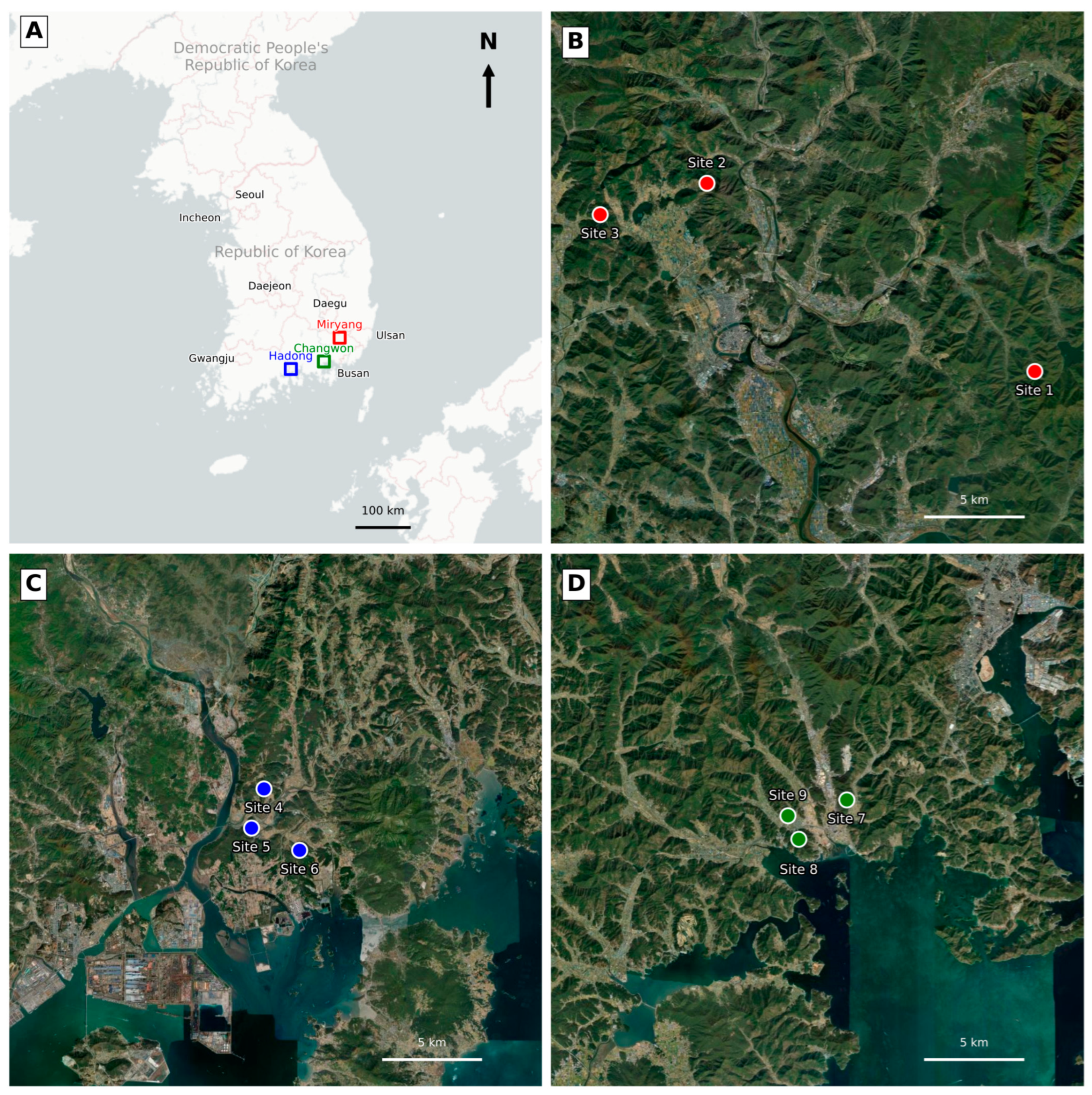
The study was conducted in pine stands in Gyeongsangnam-do, Republic of Korea, comparing three PWD management regimes: Clear-cut, Unmanaged, and Fumigation/Aerial. Clear-cut stands implemented sanitation felling to remove infection sources; Fumigation/Aerial stands involved fumigation of infected logs or decks combined with seasonal aerial insecticide application. Each regime comprised three independent sites (nine sites in total; Figure 1A–D): Sites 1–3 in Miryang (Clear-cut), Sites 4–6 in Hadong (Unmanaged), and Sites 7–9 in Changwon (Fumigation/Aerial). Site boundaries and regime color codes (red = Clear-cut; blue = Unmanaged; green = Fumigation/Aerial) are shown in Figure 1; geographic coordinates (WGS84) and locality names are provided in Table 1. To characterize baseline topographic context and assess comparability among regions (and thus among regimes), we summarized elevation, slope, and aspect for each site (Table S9). Elevation differed among regimes (one-way ANOVA; F(2, 6) = 7.271, p = 0.025), with Clear-cut sites occurring at higher elevations on average than Unmanaged and Fumigation/Aerial sites, whereas slope did not differ (F(2, 6) = 0.155, p = 0.860). Aspect is a circular variable and is therefore reported descriptively (Table S9). While elevation variation reflects constraints of the available study sites, we partly accommodated site-to-site environmental heterogeneity by including site (and plot nested within site) random effects in plot-level GLMMs (Section 2.4.6).
Figure 1.
Geographical location of the nine study sites in Gyeongsangnam-do, Republic of Korea. (A) Map of South Korea indicating the three study regions (colored boxes). A 100 km scale bar and north arrow are included for reference. (B) Miryang-si (Sites 1–3); (C) Hadong-gun (Sites 4–6); (D) Changwon-si (Sites 7–9). Colored circles indicate pine wilt disease management regimes: red = Clear-cut (Miryang); blue = Unmanaged (Hadong); green = Fumigation/Aerial (Changwon). Satellite imagery source: Esri World Imagery. Map data: © OpenStreetMap contributors and CartoDB. Design note: Regimes were assigned at the site level and were partially confounded by the geographic region (Miryang, Hadong, and Changwon). Therefore, statistical analyses (Section 2.4) treated site as the experimental unit for among-regime tests at the multivariate level and included random effects for site/plot in mixed models to maintain this hierarchy.
Table 1.
Study sites, management regimes, and coordinates (WGS84).
2.2. Field Sampling and Specimen Processing
Five plots were established at each site (25 pitfall traps per site). This within-site sampling intensity was chosen to capture fine-scale spatial heterogeneity and to stabilize site–year estimates of diversity and composition derived from pitfall catches, while remaining logistically feasible for multi-month trapping. Because management regimes were assigned at the site level, plots were treated as within-site subsamples (plot nested within site in mixed models and aggregated to the site–year level for multivariate tests); thus, among-regime inference is driven by site-level replication (three sites per regime) repeated across years rather than by plot-level replication. Annual field sampling was conducted during the primary beetle activity season. Pitfall traps were operated from April 10 to 15 October 2023, from April 10 to 10 October 2024, and from April 10 to 12 October 2025. In each plot, we installed five pitfall traps 5 m apart along a short transect or compact grid, following established guidelines for carabid sampling [22]. Each trap consisted of a plastic cup (12 cm depth, 8 cm top diameter, 5 cm bottom diameter) filled with 30% propylene glycol (PG) solution in water and installed flush with the ground. Low covers were used to protect the traps from rain and litter. PG is safe, effective, and performs well for downstream morphological and DNA-based studies [23]. The exposure period of each trap was recorded. When exposure time differed among plots or years, we standardized counts by sampling effort (trap days) during analysis (Section 2.4). Results are interpreted in terms of activity density rather than absolute population size.
To complement passive trapping (which indicates activity density), hand collection and net sweeping were conducted within each plot. All alpha and beta diversity metrics were calculated exclusively from pitfall-trap data. Active-collecting records were used solely to refine site-level species lists and functional-guild assignments; they were excluded from abundance-based metrics and all distance calculations.
The collected specimens were transported to the laboratory, processed by standard dry/wet curation, and identified to the lowest possible taxon under a stereomicroscope. Formal accession (specimen) codes were not assigned; each vial or pin was labeled with site/plot/trap metadata to uniquely identify each specimen. All voucher specimens were deposited into the Forest Protection Laboratory, Gyeongsang National University (GNU FPL), Jinju, Republic of Korea. Taxonomic identification followed the Korean Insect Name List (2021), and scientific and Korean common names were harmonized with the National Species List of Korea (2023) [24,25].
2.3. Environmental Covariate and Data Assembly
During the faunal surveys, understory vegetation cover in each plot was quantified using a consistent protocol (variable definitions and summary statistics are shown in Table S1a,b). Understory vegetation cover was measured once per year during the peak growing season, concurrent with faunal sampling, using a fixed quadrat-based protocol. Within each plot, the same trained assessor estimated the percent cover of live vascular vegetation under 1.5 m height in equal-area quadrats placed systematically around the traps. Overstory canopy and woody stems ≥1.5 m were excluded to ensure consistency across years. Overstory canopy cover/closure, soil moisture, and microclimatic conditions (e.g., temperature and humidity) were not directly measured during these surveys. Understory cover was expressed as a percentage and, for modeling, rescaled to 0–1 and z-standardized values within each year to improve convergence and comparability of effect sizes.
Raw records were compiled into a site × plot × year database containing fields for trap exposure (start/end dates), trap days, and identification notes. Quality control procedures included label–coordinate checks, scanning for missing values and extreme outliers, and internal consistency checks across duplicate entries.
2.4. Diversity Metrics and Statistical Analyses
2.4.1. Alpha Diversity (Plot-Level Generalized Linear Mixed Models, GLMMs)
For each plot and year, using pitfall-trap data only, we calculated species richness (S), Shannon diversity (H′), and total abundance (sum of individuals). We also calculated Pielou’s evenness (J) as J = H′/ln(S) to provide a standardized measure of within-assemblage structure. Active-collecting records were not included in S, H′, J, or abundance totals.
2.4.2. Why GLMMs (No Transformations)
Following best practices, count- and index-type responses were modeled using GLMMs instead of ad hoc transformations [26,27].
2.4.3. Responses and Families
Total abundance and richness (S) were modeled using a negative binomial (NB2) distribution with a log link. After verifying the approximate normality of residuals, H′ and J were modeled using Gaussian linear mixed models.
2.4.4. Effort Standardization
For count responses (abundance and S), log (trap days/100) was included as an offset; therefore, the coefficients represented differences per 100 trap days. Because multiplying all species counts within a plot by a constant does not change H′ or J, these indices were modeled directly without an offset.
2.4.5. Fixed Effects
The fixed effects were regime (three levels: Clear-cut/Unmanaged/Fumigation/Aerial), year (2023–2025), the regime × year interaction, and understory cover (scaled).
2.4.6. Random Effects
Random intercepts for site (three sites per regime) and plot nested within site accounted for the spatial hierarchy and repeated measures.
2.4.7. Estimation and Inference
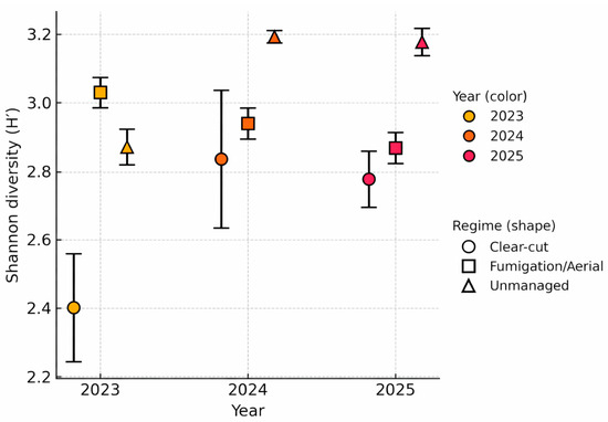
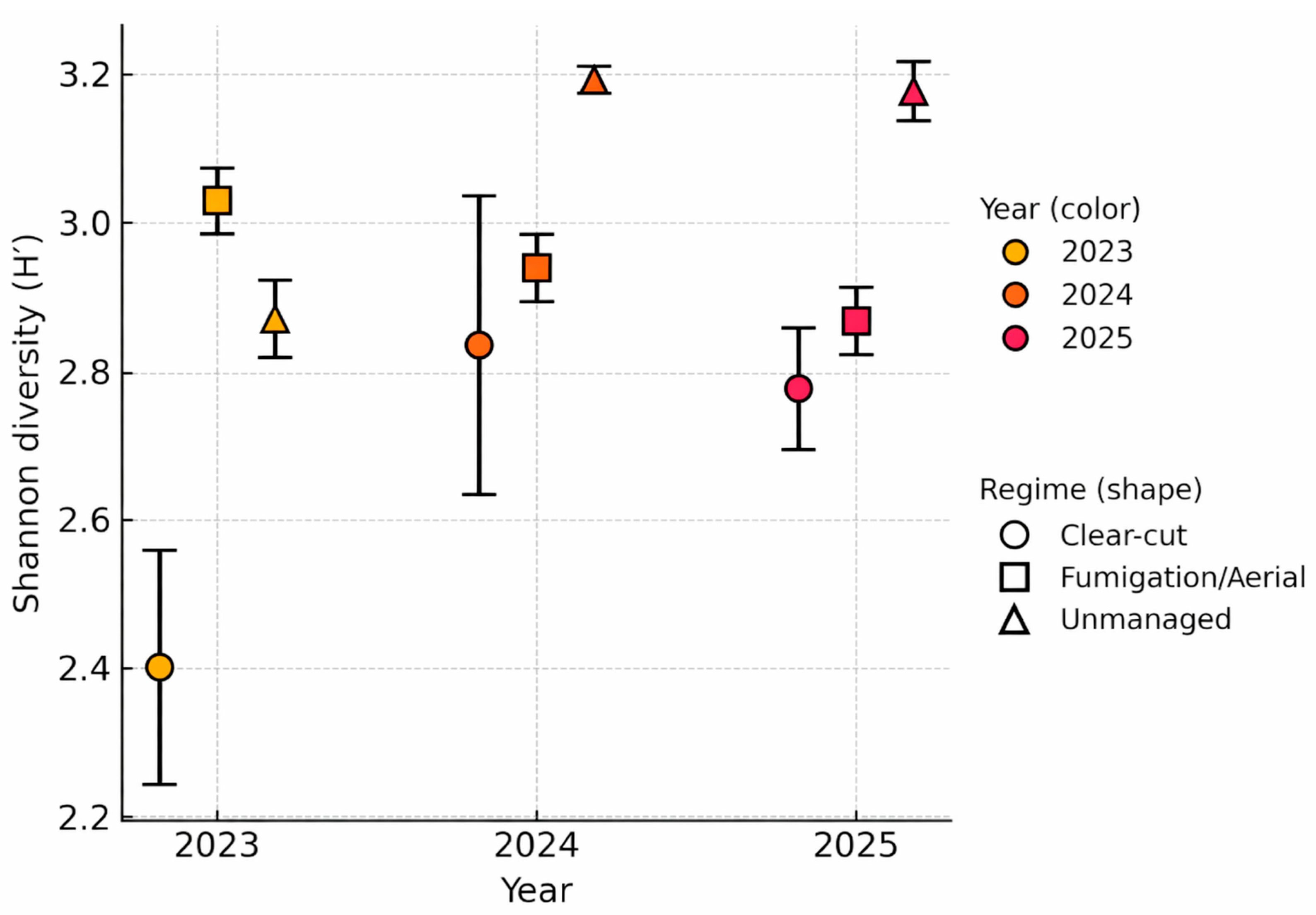
Models were fitted using the glmmTMB and lme4 packages [28,29], following Harrison et al. as a practical guide [30]. Diagnostics addressed overdispersion and zero inflation where relevant, and explanatory power was summarized using marginal/conditional R2 values [31]. Tukey-type contrasts of the estimated marginal means were computed using emmeans and multcomp [32,33]; results were displayed as compact letter displays (CLDs) [34]. For families of related tests, we controlled the false discovery rate (FDR) and reported FDR-adjusted p-values (pFDR) [35]. Point estimates with 95% confidence intervals (95% CI) were reported. Table 2 and Figure 2 summarize the main alpha diversity patterns.
Table 2.
Alpha diversity by year and management regime (pitfall-trap data only; totals standardized to 100 trap days). Values represent site-level means ± 95% CI (n = 3 sites per regime per year). Evenness (J) is Pielou’s evenness calculated as J = H′/ln(S). Superscript letters denote compact letter displays (CLDs) derived from GLMM-based Tukey contrasts within each year and metric; values sharing a letter are not significantly different at α = 0.05 after adjustment (see Table S3a–c). In 2025, the contrast between Fumigation/Aerial vs. Unmanaged stands for total abundance was non-significant.
Figure 2.
Shannon diversity (H′) of ground-active beetle assemblages by regime and year. Points show site-level means ± 95% CI (n = 3 sites per regime per year; pitfall-trap data only; totals standardized to 100 trap days). The x-axis shows survey year, the marker shape denotes regime (◯ Clear-cut; △ Fumigation/Aerial; ☐ Unmanaged), and the marker fill color indicates year (yellow = 2023, orange = 2024, red = 2025). Compact letter displays were removed to avoid confusion with Table 2; see Table 2 and Table S3a–c for inferential details. Source: Authors’ own work.
2.4.8. Beta Diversity (Site-Level Permutational Multivariate Analysis of Variance, PERMANOVA, and Ordination)
Because regimes were assigned at the site level, among-regime differences in composition at the site–year level were examined to avoid pseudoreplication. For each site–year, pitfall-trap data only were aggregated, trap day–standardized abundances were summed across the five plots, and a square-root transformation was applied before computing distances.
2.4.9. Dissimilarity and Ordination
Among-sample dissimilarity was quantified using Bray–Curtis distances [19], and community structure was visualized using principal coordinate analysis (PCoA) [20]. Axis contributions (percent variance) were shown on the ordination plots.
2.4.10. Hypothesis Tests (Year by Year)
A one-way PERMANOVA [21] was performed separately for each year (n = 9 site samples per year; 3 per regime) with 999 permutations, using management regime as the sole factor. Homogeneity of multivariate dispersion was evaluated using the permutation test for homogeneity of multivariate dispersion (PERMDISP) [35], and no contradictions in the PERMANOVA inferences were detected.
2.4.11. Sensitivity Analyses and Constrained Ordinations
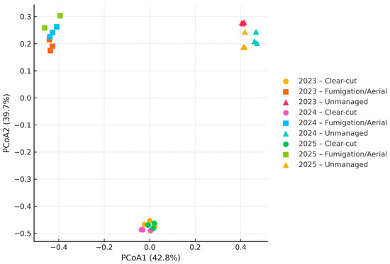
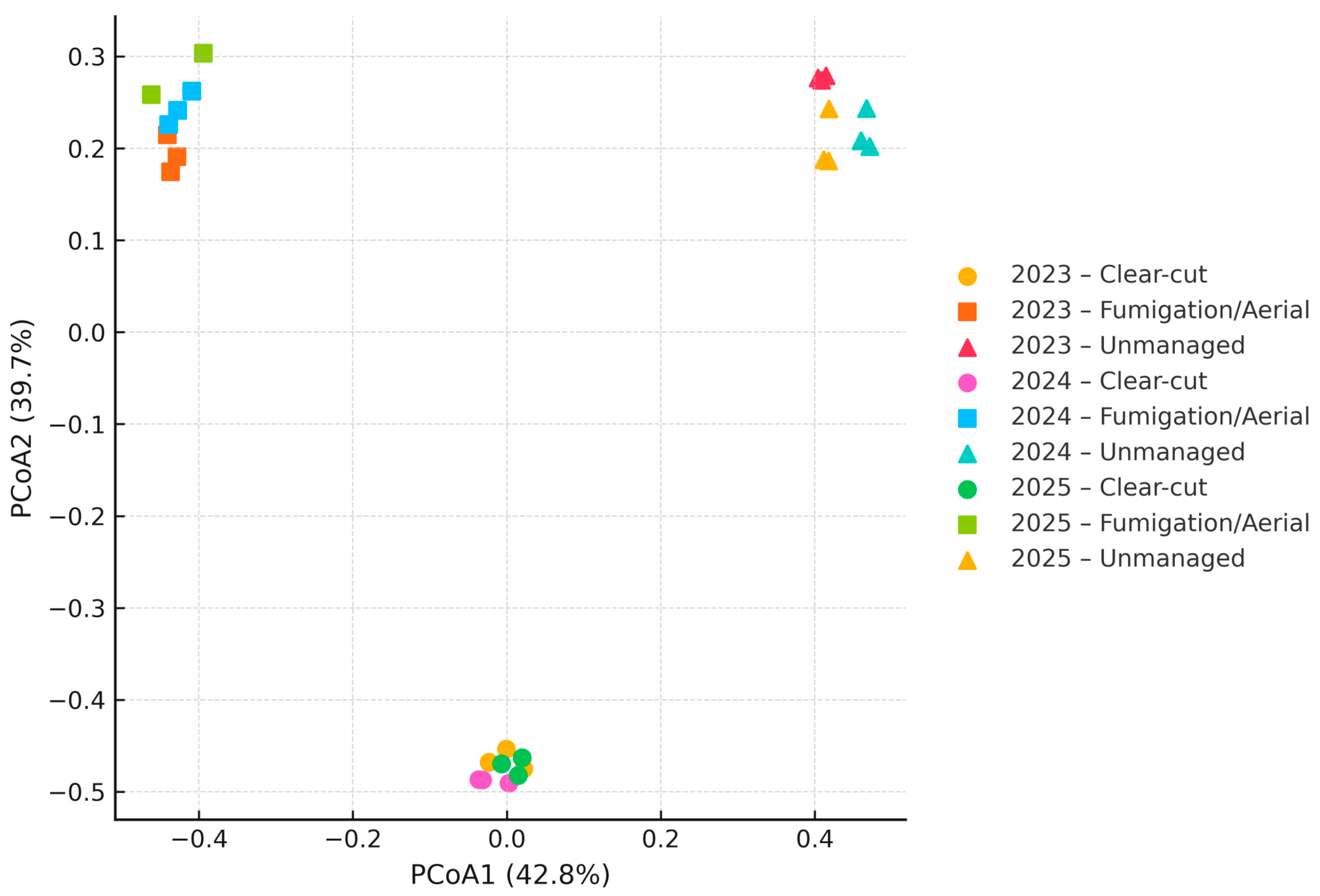
PERMANOVA was repeated after applying a Hellinger transformation [36], and qualitatively identical conclusions were obtained. In addition, to explicitly visualize species–regime associations in a constrained ordination framework, we conducted a redundancy analysis (RDA) using the site–year species matrix derived from pitfall-trap data only (see Section 2.4.8). For each site–year, abundances were standardized by sampling effort (trap days) and aggregated across plots prior to ordination, and the resulting community matrix was Hellinger-transformed to support Euclidean-based ordination of species data [36]. Management regime was used as the constraining factor, and the RDA biplot is provided as Figure S2; for readability, only representative taxa are labeled in the biplot (see the species key in Figure S2). As a complementary constrained ordination that incorporates an environmental covariate, a canonical analysis of principal coordinates (CAP) was also conducted, including understory cover as a covariate [37]; CAP outputs are provided in the Supplementary Information. Figure 3 presents the PCoA biplots, and Table 3 lists the PERMANOVA results (F, df, R2, p).
Figure 3.
Principal coordinates analysis (PCoA) of Bray–Curtis dissimilarities among site–year beetle assemblages (pitfall-trap data only; abundances square-root transformed; totals standardized to 100 trap days). Symbols denote management regimes (circles = Clear-cut; squares = Fumigation/Aerial; triangles = Unmanaged); colors denote years (2023, 2024, 2025) as in the legend. Each year includes n = 9 site samples (3 per regime). Axis labels indicate the proportion of variance explained (PCoA1 = 42.8%, PCoA2 = 39.7%). Year-specific PERMANOVA results are provided in Table 3 (999 permutations per year; R2 = 0.970–0.983). Source: Authors’ own work.
Table 3.
Permutational multivariate analysis of variance (PERMANOVA; Bray–Curtis) results by year on site-level community matrices (pitfall-trap data only; abundances square-root transformed). Permutation-based p-values were calculated using 999 permutations per year; degrees of freedom and sample size (N) are shown for each year. R2 values are the coefficients of determination returned by the PERMANOVA routine and represent the proportion of among-sample variation in Bray–Curtis dissimilarities explained by regime.
2.4.12. Functional Composition and Top-Species Displays
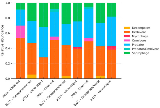
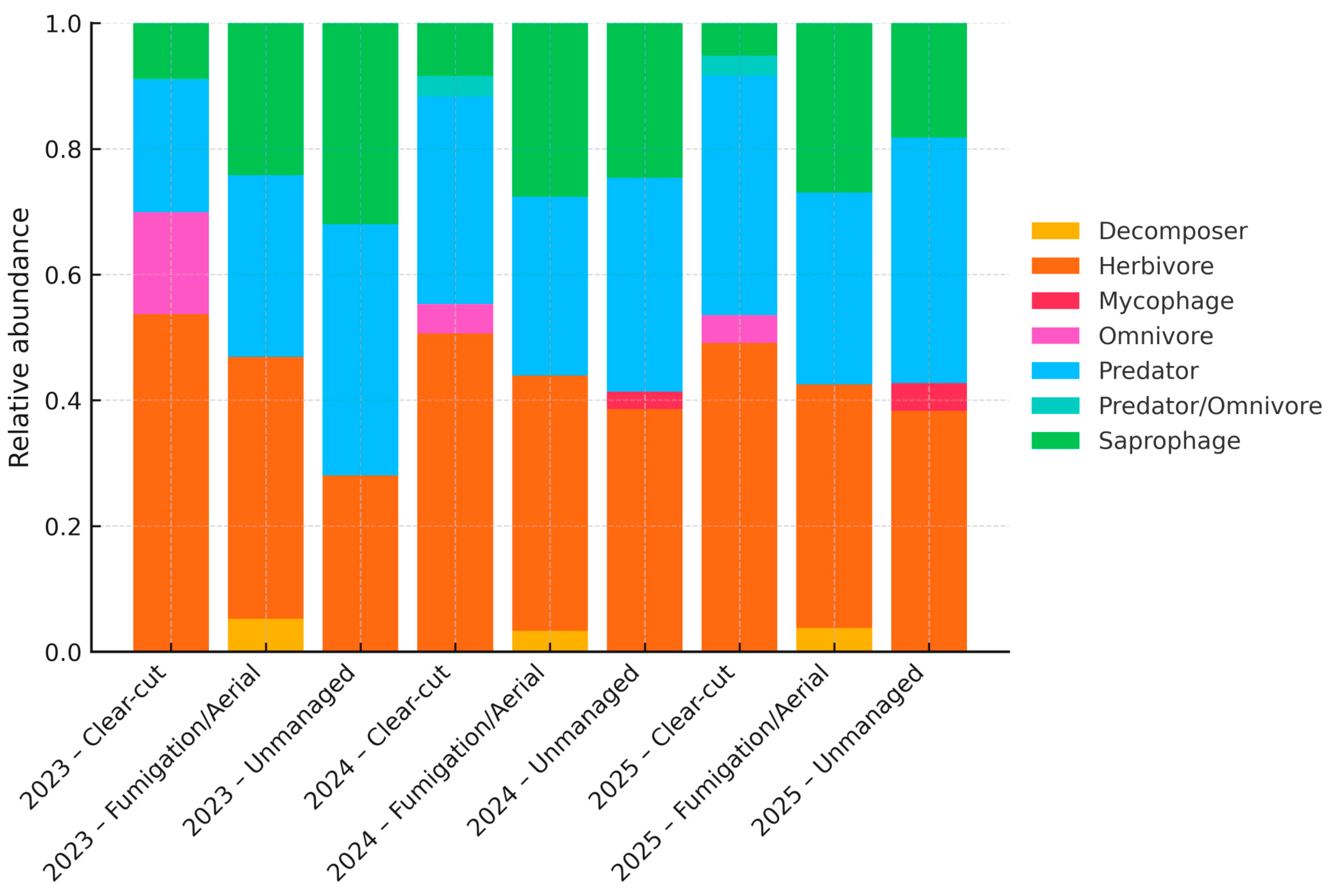
Each species was assigned to one of seven functional guilds using a curated mapping (Table S2a): decomposer (litter/substrate processors), herbivore (phytophagous), mycophage (fungus feeders), omnivore (non-predatory generalists), predator (primarily carnivorous), predator/omnivore (mixed feeding including predation), and saprophage (detritivores consuming decaying organic matter, including many dead-wood-associated taxa). Because some guild categories were rare (e.g., mycophages) and a small subset of taxa had uncertain or ambiguous guild identities, guild-level patterns for rare/uncertain categories should be interpreted cautiously; ambiguous cases and QA notes are documented in Table S2b. For each year × regime combination, the relative composition (0–1) was calculated from pitfall-trap data only (totals standardized to 100 trap days), ensuring that each column sums to 1.0. Figure 4 shows the stacked bars, and Table 4 lists the corresponding percentages.
Figure 4.
Relative functional guild composition of ground-active beetle assemblages by year and management regime. Stacked bars show the proportion (0–1) of seven guilds, decomposer, herbivore, mycophage, omnivore, predator, predator/omnivore, and saprophage, for each year × regime combination (left to right: 2023, 2024, 2025 × Clear-cut, Fumigation/Aerial, Unmanaged). Values are based on pitfall-trap data only; totals were standardized to 100 trap days and aggregated within each year × regime. Columns sum to 1.0 (100%). Colors follow the legend. The corresponding percentages are reported in Table 4, and species-to-guild assignments are provided in Table S2a (see Table S4 for the collapsed four-guild summary). Source: Authors’ own work.
Table 4.
Functional guild composition (relative abundance, %) by year and management regime.
To facilitate comparison with studies that use four categories, a collapsed summary is included in the Supplementary Materials (Table S4) with the following mapping: phytophagous = herbivore; predatory = predator + predator/omnivore; saproxylic ≈ saprophage; detritivorous = decomposer + mycophage + omnivore. The seven-guild scheme is used in all main-text figures and tables.
2.4.13. Indicator Species Analysis
Indicator value (IndVal) scores were computed for each year and regime using the Dufrêne–Legendre approach and permutation tests in indicspecies [38,39,40]. Tables report IndVal scores and permutation-based p-values.
2.4.14. Software and Reproducibility
The analyses were performed using a hybrid Python–R workflow. Data assembly, diversity-metric calculations (alpha and beta diversity), and all beta diversity analyses (PCoA, PERMANOVA, PERMDISP, and CAP) were conducted in Python (version 3.13; Python Software Foundation, Beaverton, OR, USA) [41] using the SciPy ecosystem, primarily pandas, scikit-bio, SciPy, and Matplotlib [42,43,44,45]. Alpha diversity responses were modeled in R (version 4.4.1, 2024; R Core Team, Vienna, Austria) [46] using glmmTMB and lme4 to fit GLMMs [28,29]. Post hoc contrasts and estimated marginal means were computed using emmeans and multcomp [32,33], and model diagnostics were performed with performance [47]. Statistical significance was assessed at α = 0.05. For families of related tests (e.g., across alpha diversity responses), false discovery rate control was applied [35]. The code and reproducible workflow are available upon request. Tables S1 and S2 describe the data fields required to reproduce the analyses. To evaluate sampling adequacy, we constructed sample-based species accumulation curves for each management regime using site–year as the sampling unit (n = 9 per regime; 3 sites × 3 years), based on pitfall-trap data only (Figure S1). Sample order was randomized 999 times within each regime, and we report the mean cumulative species richness with 95% confidence intervals (2.5–97.5th percentiles) across permutations. Sampling completeness was also assessed using Good’s coverage [48]; values are reported in Table S8.
2.5. Notes on Inference and Limitations
As regimes are not cross-classified with geographic region, unmeasured regional differences may covary with regime. This design, therefore, fundamentally restricts causal inference; statistical controls can reduce, but cannot fully remove, region–regime confounding. This was addressed in three ways: (i) regime differences in composition were tested at the site–year level, (ii) site/plot random effects were included in plot-level GLMMs to account for the hierarchy, and (iii) we explicitly modeled understory cover as a covariate. These design features are highlighted to guide interpretation and to encourage future studies that orthogonally balance regimes and regions. Finally, this partial confounding likely contributes to the very high PERMANOVA R2 values (0.970–0.983) reported in Section 3.2; accordingly, these separations are interpreted as region-structured, regime-associated differences rather than strictly causal regime effects. Consistent with this limitation, baseline topographic context differed among regions; elevation differed among regimes (F(2, 6) = 7.271, p = 0.025; Table S9), whereas slope did not (F(2, 6) = 0.155, p = 0.860). Aspect is reported descriptively (Table S9), reinforcing that regime-associated patterns may partly reflect unmeasured regional gradients.
3. Results
3.1. Alpha Diversity Across Regimes and Years
Across the 3 years, Unmanaged stands generally supported the highest species richness and, in two of the three years, the highest Shannon diversity (H′), whereas Fumigation/Aerial stands consistently exhibited the highest mean total abundance (Figure 2). Pielou’s evenness (J) was generally high across regimes and years and differed more modestly than richness and H′ (Table 2). Sampling adequacy was supported by the sample-based species accumulation curves, which showed diminishing returns and approached asymptotes within each regime (Figure S1), consistent with the high Good’s coverage values across regimes and years (typically ≥ 0.95; Table S8), suggesting that the observed among-regime patterns are unlikely to be driven by undersampling artifacts.
In 2023, post hoc contrasts (CLDs; Table S3) indicated three statistically distinct groups for all three metrics (that is, all pairwise differences among Clear-cut, Fumigation/Aerial, and Unmanaged regimes were significant). Species richness was the highest in Unmanaged stands, whereas total abundance and H′ were the highest in Fumigation/Aerial stands (e.g., abundance = 228.67 ± 24.38; H′ = 3.03 ± 0.04). Pairwise richness ratios were Clear-cut vs. Fumigation/Aerial = 0.67 (padj < 0.001), Clear-cut vs. Unmanaged = 0.62 (padj < 0.001), and Fumigation/Aerial vs. Unmanaged = 0.92 (padj = 0.029).
These patterns shifted in the subsequent years. In 2024, Unmanaged stands (mean = 29.33 ± 1.43) had significantly greater richness than the other two regimes in richness, whereas Clear-cut and Fumigation/Aerial stands were statistically indistinguishable (ratio = 1.00, padj = 1.000). By contrast, H′ and total abundance were separated into three groups: abundance again peaked in Fumigation/Aerial stands (220.67 ± 3.79), whereas H′ peaked in Unmanaged stands (3.19 ± 0.02). In 2025, Unmanaged stands again exceeded both Clear-cut and Fumigation/Aerial stands in terms of richness, and the latter two did not differ from each other (ratio = 0.97, padj = 0.532). H′ was the highest in Unmanaged stands (3.18 ± 0.04), and total abundance was the highest in Fumigation/Aerial stands (237.33 ± 11.47), although the Fumigation/Aerial vs. Unmanaged stand abundance contrast was non-significant in 2025 (Table S3).
Full post hoc pairwise comparisons for all metrics and years (effect–size ratios and adjusted padj values) are provided in Table S3. Together, these year-to-year shifts confirm a significant regime × year interaction (Table 2): Clear-cut stands exhibited the lowest diversity shortly after cutting, Fumigation/Aerial stands consistently sustained the highest activity density (abundance), and Unmanaged stands achieved the greatest richness and Shannon diversity (H′) in later years. Evenness (J) remained high overall and showed comparatively smaller among-regime differences. Understory vegetation cover showed weak to moderate positive associations with richness and H′ but was generally less influential than regime and only occasionally reached statistical significance. These regime contrasts should be interpreted cautiously because management regime is partially confounded with region (Section 2.5).
3.2. Community Composition (PCoA and PERMANOVA)
PCoA of Bray–Curtis dissimilarities showed distinct regime groupings within each year (Figure 3). Year-specific PERMANOVAs (999 permutations per year) indicated significant differences among management regimes in all 3 years (2023: F(2, 6) = 177.36, p = 0.003; 2024: F(2, 6) = 133.64, p = 0.007; 2025: F(2, 6) = 97.17, p = 0.007; N = 9 per year).
The R2 values were exceptionally high (0.970–0.983), indicating strong and distinct separation among the three groups (Table 3). These high R2 values likely reflect both strong regime-associated structuring and distinct geographic and environmental differences among the three regions (Miryang, Hadong, and Changwon) where each regime was applied (see Section 2.1 and Section 2.5), as regime is partially confounded with region. Tests for homogeneity of multivariate dispersion (PERMDISP) did not reveal dispersion differences that would contradict these inferences. Finally, the first two PCoA axes together accounted for a substantial share of the among-sample variation (axis contributions are shown in Figure 3). A complementary redundancy analysis (RDA) on the Hellinger-transformed site–year matrix showed a regime separation consistent with the PCoA results and highlighted regime-associated taxa in constrained ordination space (Figure S2). For example, open-habitat carabids such as Dolichus halensis and Harpalus sinicus were positioned toward Clear-cut stands, whereas Pheropsophus jessoensis and Prionus insularis were positioned toward Fumigation/Aerial stands, consistent with the dominant and indicator taxa patterns reported below (Section 3.4; Figure 5; Table S6). In the constrained ordination (CAP), understory cover explained a modest additional fraction of compositional variation beyond regime (Supplementary CAP outputs). For each site, among-year Bray–Curtis dissimilarities were quantified using abundances standardized to 100 trap days. The mean within-regime temporal turnover was the highest in Clear-cut stands (2023–2025:0.647 [0.628–0.659]), intermediate in Unmanaged stands (0.384 [0.345–0.448]), and the lowest in Fumigation/Aerial stands (0.193 [0.180–0.217]) (Table S7). This pattern is consistent with strong postharvest successional changes following cutting and relative assemblage stability under canopy retention.
Figure 5.
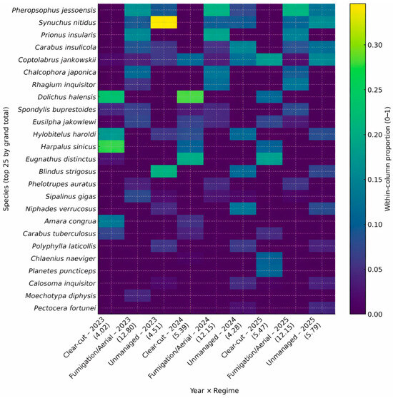
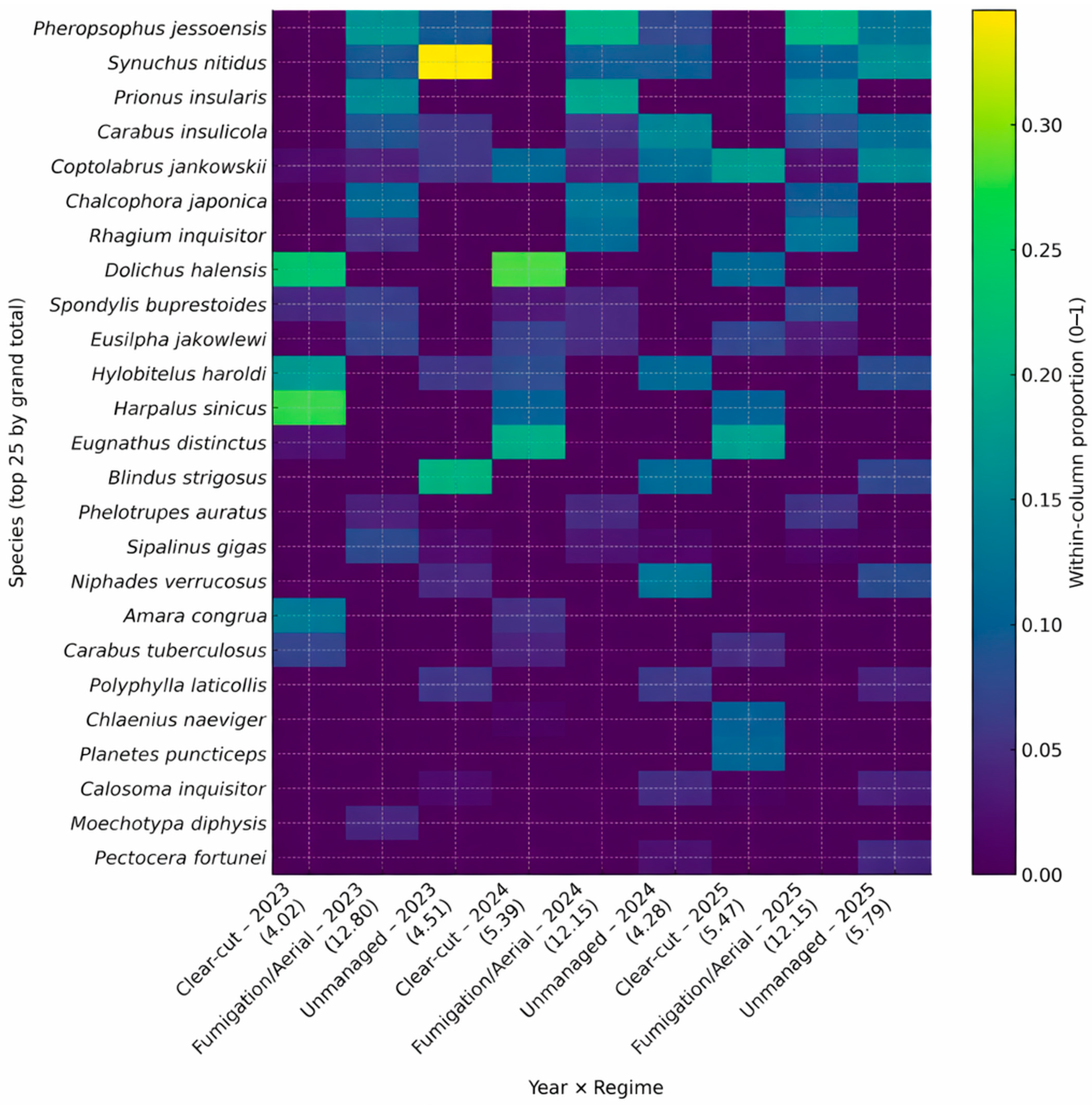
Relative-abundance heatmap for the top 25 beetle species across year × regime combinations. Columns are grouped by year (2023, 2024, 2025) and labeled as regime–year (Clear-cut, Fumigation/Aerial, Unmanaged). Cell color indicates the within-column proportion (0–1; color bar at right), where each column sums to 1.0. Numbers in parentheses under the x-axis labels denote the total standardized abundance (per 100 trap-days) for that year × regime combination. Species names are listed on the left.
3.3. Functional Composition
The year × regime combination showed distinct functional guild profiles (Table 4; Figure 4). In 2023, Unmanaged stands had the highest share of saprophage and predator guilds. This pattern shifted in 2024–2025. The predatory share (collapsed four-guild category: predator + predator/omnivore) was highest in Clear-cut stands, whereas the saproxylic/saprophage share was highest in Fumigation/Aerial stands; however, all three regimes retained distinct functional profiles across years. Clear-cut stands consistently favored phytophagous (herbivore) and detritivorous components (decomposer + mycophage + omnivore), particularly soon after harvest, whereas Fumigation/Aerial stands tended to be intermediate for most guilds, aside from the saproxylic peak noted above. Percent values for each year × regime column (summing to 100%) are provided in Table 4 and correspond to the stacked bars in Figure 4; the collapsed four-guild summaries supporting the cross-year maxima are provided in Table S4.
3.4. Top-Species Patterns
The relative-abundance heatmap of the 25 most abundant beetle species revealed clear regime- and year-specific dominance patterns (Figure 5). Rows in Figure 5 are ordered by the grand total standardized abundance (summed across all year × regime combinations; individuals per 100 trap-days), placing the most abundant species at the top. Within each year × regime column, cell colors represent within-column relative abundances (i.e., proportions summing to 1.0 per column).
Several species revealed pronounced peaks in specific regimes and years. For example, Pheropsophus jessoensis and Prionus insularis were consistently dominant in Fumigation/Aerial stands across all three years. In contrast, Synuchus nitidus reached very high relative abundances in Unmanaged stands in 2023 and remained common in both fumigation and unmanaged stands in later years. Open-habitat carabids such as Dolichus halensis and Harpalus sinicus were strongly associated with Clear-cut stands, especially in 2023–2024. Meanwhile, forest-associated taxa, including Carabus insulicola, and Blindus strigosus, showed high relative dominance in Unmanaged stands. Other species, such as Chalcophora japonica in Fumigation/Aerial stands and Coptolabrus jankowskii in Clear-cut and Unmanaged stands during 2024–2025, also exhibited distinct regime- and year-specific peaks.
Table 5 summarizes standardized abundances (individuals per 100 trap-days) for the top 15 species, following the ranking order in Figure 5. The complete matrices of standardized abundances and corresponding within-column proportions for all 31 species are provided in Tables S5a and S5b, respectively. IndVal analysis further identified regime-specific indicator taxa for each year (permutation tests within year; n = 9 stands per year). In Fumigation/Aerial stands, Pheropsophus jessoensis was a consistent indicator (e.g., 2023: IndVal = 0.825, p = 0.006; 2025: IndVal = 0.761, p = 0.004). Clear-cut stands were characterized by early-successional or open-habitat carabids (e.g., Carabus tuberculosus; 2023: IndVal = 1.000, p = 0.022), whereas Unmanaged stands showed high fidelity of forest-associated taxa (e.g., Blindus strigosus; 2023: IndVal = 1.000, p = 0.016). Given the partial confounding of management regime with region, these patterns should be interpreted as evidence of regime-structured assemblages rather than strictly causal regime effects; full indicator-value rankings are in Table S6.
Table 5.
Top 15 beetle species by standardized abundance (individuals per 100 pitfall trap-days) in pitfall traps for each year × regime combination. Values are based on pitfall trap data only; catches were standardized to 100 trap-days before aggregation. Species are ordered as in Figure 5 (descending grand total).
4. Discussion
4.1. Synthesis of Alpha and Beta Diversity Responses Across Control Regimes
The 3-year findings show that Unmanaged stands consistently supported higher species richness, and in two of the three years, higher Shannon diversity (H′), whereas Fumigation/Aerial stands maintained the highest total abundance. Pielou’s evenness (J) provided a standardized view of within-assemblage structure and indicated generally high evenness across regimes, with comparatively smaller between-regime contrasts than richness and H′ (Table 2). Clear-cut stands generally had the lowest richness and H′ immediately after cutting (Table 2; Figure 2). This pattern aligns with long-standing evidence that structural simplification and microclimatic extremes following intensive harvest reduce the diversity of ground-active beetles in the short term [14,15,16,17]. In contrast, retaining an overstory structure, even when chemical control is used, can sustain activity density (abundance), likely by preserving litter continuity and movement corridors, while filtering sensitive taxa and shaping Shannon diversity (H′) and evenness (J). The significant regime × year interaction indicates dynamic trajectories; as the understory develops, partial recovery of alpha diversity in Clear-cut stands is expected, consistent with post-harvest successional responses reported in previous studies [14,15,16,17].
This compositional separation was also evident in the multivariate space: PCoA showed distinct regime groupings within each year, and year-specific one-way PERMANOVA detected significant differences among management regimes in all three years (Table 3; Figure 3). Importantly, the exceptionally high R2 values (0.970–0.983) reported in Section 3.2 likely reflect not only strong separation among regimes, but also the partial confounding of regime with geographic region (Miryang, Hadong, and Changwon), as noted in Section 2.1 and Section 2.5. Because PERMDISP results revealed no among-regime differences in multivariate dispersion, we interpreted the separation primarily as a centroid (compositional) shift rather than a dispersion artifact [21,49]; that is, commonly used PWD control regimes are associated with distinct assemblage states, not merely differences in variability among samples.
4.2. Functional Composition and Plausible Mechanisms
The observed diversity patterns appear to reflect shifts in functional guild composition (Table 4; Figure 4). In 2023, Unmanaged stands showed the highest relative contributions of saprophage and predator guilds, consistent with greater availability of deadwood, shaded litter, and structurally complex microsites that support both wood-dependent taxa and higher trophic levels [10,12,14,15,16,17]. In 2024–2025, this pattern shifted: predatory shares peaked in Clear-cut stands, whereas saproxylic/saprophage components were the highest in Fumigation/Aerial stands, and Unmanaged stands retained comparatively balanced profiles (Table 4; Figure 4). By contrast, Clear-cut stands consistently had higher shares of early-successional guilds, particularly herbivore and omnivore, in the initial post-harvest years, and Fumigation/Aerial stands tended to be intermediate for most guilds overall, consistent with canopy retention and potential non-target suppression associated with chemical control [5,6,7]. The top-species heatmap (Table 5; Figure 5) complements these patterns by revealing regime-specific dominants that act as indicator-like taxa; such signals are commonly observed when habitat filters (e.g., deadwood amount, shade, litter continuity) vary among regimes [11,12,13,14,15,16,17].
Although understory vegetation cover was included as a covariate, the multi-year compositional shifts, particularly in Clear-cut stands, are consistent with a mediation pathway in which understory development gradually moderates the microclimate and restores resource heterogeneity. Interannual climatic variability (e.g., regional temperature and rainfall) can influence beetle phenology and activity and, thus, pitfall-trap-derived guild proportions; hence, some of the observed year-to-year guild shifts may reflect climate-driven differences in activity. In the absence of explicit meteorological covariates, we interpret these temporal patterns cautiously. This interpretation aligns with experimental and synthesis studies showing that the retention of structure and microclimate buffering reduces the magnitude and duration of post-harvest biodiversity losses [50,51]. Future path analyses or structural equation models could help quantify the relative contributions of regimes versus vegetation covariates to alpha and beta diversity.
4.3. Implications for Sustainable PWD Management
Building on these functional shifts, our results suggest several principles for sustainable management of PWD. First, where sanitation felling is unavoidable, reducing harvest intensity and adopting retention forestry, leaving patches or strips of live trees, legacy logs, and vertical elements, can buffer microclimates and maintain key resources for non-target beetles [50,51]. In PWD-affected landscapes, recent studies suggest practical targets, such as retaining ≥30% canopy cover and 20–30 m3 ha−1 of deadwood, to maintain assemblage functions while disease control measures are applied [50,51,52]. Under strict sanitation mandates, these targets may not be achievable within the sanitation core; therefore, retention should focus on regulation-compliant, low-risk material (e.g., non-infested and/or appropriately treated substrate) and, where needed, be implemented at patch/compartment or landscape scales. However, these values should be considered starting points rather than fixed prescriptions; local calibration by climate, stand age, slope/terrain, and broader landscape context is recommended before adoption [50]. Second, saproxylic diversity responds strongly to deadwood quantity and configuration. Managers should retain or import deadwood of varied sizes and positions (standing and downed), as stumps alone are rarely sufficient to offset habitat losses under intensified stump harvesting [53,54]. Third, because aerial insecticides can suppress non-target arthropods [5,6,7], IPM emphasizing targeted applications and complementary biological or plant-derived tools may reduce ecological side effects while supporting disease control [54,55,56]. Finally, remote sensing and machine learning can support routine monitoring and evaluation by mapping PWD risk and prioritizing sites for intervention [57]. Such risk-based targeting may reduce unnecessary disturbance while maintaining sanitary objectives.
4.4. Methodological Considerations and Study Limitations
The replicated three-year design, with standardized passive (pitfall) and supplemental active sampling across sites, supports robust inference about differences among regimes within the studied regions. We note two caveats. First, pitfall traps quantify activity density rather than absolute population size, and capture rates can vary with microclimate and behavior [11,12,13,22,23]. Accordingly, abundance results are interpreted as activity density (see Methods). Active hand collection and net sweeping were used only to refine species lists and functional guild assignments and were excluded from all alpha and beta diversity calculations. Second, regimes were assigned at the site level and partially confounded with region; therefore, broader generalizations beyond southern Korea should consider climatic variability, stand age, and landscape context. These limitations suggest useful extensions, such as adding pre-/post-control baselines, co-measuring microclimates and soils, and expanding to multi-taxon assessments (e.g., spiders and other arthropod guilds).
5. Conclusions
The 3-year evidence obtained in this study shows that widely deployed PWD control options are consistently associated with distinct ground-active beetle assemblages along a management gradient. The stark contrast between the high total abundance under Fumigation/Aerial control and higher richness and Shannon diversity (H′) in Unmanaged stands, together with generally high evenness (J) and the recurrent compositional separation among regimes, underscores the importance of retaining structures and deadwood when applying control. Integrating these biodiversity safeguards into PWD programs is crucial for improving the ratio of disease control benefit to ecological cost, thereby advancing sustainable forest management goals in PWD-affected landscapes [11,12,13,14,15,16,17,50,51,53,54].
Future research should (i) adopt orthogonally replicated, multi-region designs with pre-regime baselines using before–after–control–impact (BACI/BACIPS) frameworks to strengthen causal inference [58,59]; (ii) extend monitoring beyond three years and pair standardized pitfall sampling with measurements of microclimate, understory vegetation, and deadwood to test mechanistic pathways; (iii) broaden taxonomic coverage by combining morphology with DNA-based approaches—including metabarcoding of bulk tissue and trap preservatives (e.g., ethanol or PG)—to detect cryptic taxa and accelerate processing [57,60,61]; (iv) experimentally vary retention levels to calibrate locally actionable thresholds for canopy and deadwood; and (v) integrate biodiversity outcomes with risk mapping using remote sensing and machine learning to target control where the benefit-to-cost ratio is the highest [57].
Policy note: Numeric retention targets (e.g., ≥30% canopy cover; 20–30 m3 ha−1 deadwood) are grounded in experimental/synthesis work [50,51,52,53,54] but should be adapted to local conditions—including climate, stand age, slope/terrain, and landscape context—prior to operational use.
Supplementary Materials
The following supporting information can be downloaded at: https://www.mdpi.com/article/10.3390/su18031244/s1, Figure S1: Sample-based species accumulation curves (999 permutations; 95% CI) by management regime; Figure S2: Redundancy analysis (RDA) biplot of Hellinger-transformed site–year assemblages showing species–regime associations; Table S1a: Understory vegetation cover—site × year raw records; Table S1b: Understory vegetation cover—year × regime summary; Table S2a: Species-to-guild mapping (seven categories; final assignments used in analyses); Table S2b: Conflicts to review (multiple or uncertain guild assignments; QA log); Table S3a: Shannon diversity—GLMM Tukey/FDR post hoc p-values and contrasts; Table S3b: Species richness—GLMM post hoc ratios; Table S3c: Total abundance—GLMM post hoc ratios; Table S4: Four-guild composition by year × regime; columns sum to 100%; Table S5a: Species × year × regime matrix (standardized to 100 trap days; summed across sites); Table S5b: Species × year × regime matrix (column-normalized proportions); Table S6: Indicator species analysis: IndVal and permutation p-values; Table S7: Within-regime temporal turnover; Bray–Curtis for the 2023–2025 comparisons per site; Table S8: Good’s coverage by regime × year; Table S9: Topographic context of study sites by management regime (elevation, slope, and aspect).
Author Contributions
Conceptualization, C.K.L., H.K. and M.-L.H.; data curation, M.-L.H.; formal analysis, H.K. and M.-L.H.; investigation, C.K.L. and M.-L.H.; methodology, C.K.L. and H.K.; project administration, C.K.L. and H.K.; resources, C.K.L. and M.-L.H.; software, H.K. and M.-L.H.; supervision, C.K.L. and H.K.; validation, M.-L.H.; visualization, H.K. and M.-L.H.; writing—original draft, M.-L.H.; writing—review and editing, H.K. All authors have read and agreed to the published version of the manuscript.
Funding
This study received no external funding.
Institutional Review Board Statement
Not applicable.
Informed Consent Statement
Not applicable.
Data Availability Statement
The original contributions presented in the study are included in this article and its Supplementary Materials (Figures S1 and S2 and Tables S1–S9). Further inquiries can be directed to the corresponding author.
Conflicts of Interest
The authors declare no conflicts of interest.
Abbreviations
The following abbreviations are used in this manuscript:
| CAP | canonical analysis of principal coordinates |
| CI | confidence interval |
| CLD | compact letter display |
| CWD | coarse woody debris |
| FDR | false discovery rate |
| GLMM | generalized linear mixed model |
| IndVal | indicator value index |
| IPM | integrated pest management |
| M&E | monitoring and evaluation |
| NB2 | negative binomial (type 2; quadratic variance) |
| PCoA | principal coordinates analysis |
| RDA | redundancy analysis |
| PERMANOVA | permutational multivariate analysis of variance |
| PERMDISP | permutation test for homogeneity of multivariate dispersion |
| PG | propylene glycol |
| PWD | pine wilt disease |
| H′ | Shannon diversity |
| S | species richness |
| p, pFDR | p-value and FDR-adjusted p-value |
| n | sample size |
| R2 | coefficient of determination |
| α | significance level |
| df_between | degrees of freedom (between) |
| df_within | degrees of freedom (within) |
| Year × regime | interaction term |
References
- Back, M.A.; Bonifácio, L.; Inácio, M.L.; Mota, M.; Boa, E. Pine wilt disease: A global threat to forestry. Plant Pathol. 2024, 73, 1026–1041. [Google Scholar] [CrossRef] [Scilit]
- Kobayashi, F.; Yamane, A.; Ikeda, T. The Japanese pine sawyer beetle as the vector of pine wilt disease. Annu. Rev. Entomol. 1984, 29, 115–135. [Google Scholar] [CrossRef]
- Kwon, T.-S.; Shin, J.H.; Lim, J.-H.; Kim, Y.-K.; Lee, E.J. Management of pine wilt disease in Korea through preventative silvicultural control. For. Ecol. Manag. 2011, 261, 562–569. [Google Scholar] [CrossRef] [Scilit]
- Republic of Korea. Special Act on the Extermination of Pine Wilt Disease; Act No. 7549, 31 May 2005 (as amended); Korea Legislation Research Institute: Sejong City, Republic of Korea, 2005; Available online: https://faolex.fao.org/docs/pdf/kor166848.pdf (accessed on 1 November 2025).
- Kwon, T.-S.; Song, M.-Y.; Shin, S.-C.; Park, Y.-S. Effects of aerial insecticide sprays on ant communities to control pine wilt disease in Korean pine forests. Appl. Entomol. Zool. 2005, 40, 563–574. [Google Scholar] [CrossRef] [Scilit]
- Suh, D.Y.; Jung, J.-K.; Lee, S.K.; Seo, S.-T. Effect of aerial spraying of thiacloprid on pine sawyer beetles (Monochamus alternatus) and honey bees (Apis mellifera) in pine forests. Entomol. Res. 2021, 51, 83–89. [Google Scholar] [CrossRef] [Scilit]
- Kwon, T.-S. Change of abundance of arthropods in pine forests caused by aerial insecticide spray. Arch. Environ. Contam. Toxicol. 2008, 54, 92–106. [Google Scholar] [CrossRef] [Scilit]
- Park, Y.-S.; Park, Y.K.; Yang, H.M. Effects of clear-cutting on forest arthropod communities at two different vertical levels (crown and ground surface). Korean J. Ecol. Environ. 2016, 49, 271–278. [Google Scholar] [CrossRef] [Scilit]
- Hartshorn, J.A. A review of forest management effects on terrestrial leaf litter inhabiting arthropods. Forests 2020, 12, 23. [Google Scholar] [CrossRef] [Scilit]
- Stokland, J.N.; Siitonen, J.; Jonsson, B.G. Biodiversity in Dead Wood; Cambridge University Press: Cambridge, UK, 2012. [Google Scholar] [CrossRef] [Scilit]
- Rainio, J.; Niemelä, J. Ground beetles (Coleoptera: Carabidae) as bioindicators. Biodivers. Conserv. 2003, 12, 487–506. [Google Scholar] [CrossRef] [Scilit]
- Pearce, J.L.; Venier, L.A. The use of ground beetles (Coleoptera: Carabidae) and spiders (Araneae) as bioindicators of sustainable forest management: A review. Ecol. Indic. 2006, 6, 780–793. [Google Scholar] [CrossRef] [Scilit]
- Koivula, M.J. Useful model organisms, indicators, or both? Ground beetles (Coleoptera, Carabidae) reflecting environmental conditions. ZooKeys 2011, 100, 287–317. [Google Scholar] [CrossRef] [Scilit]
- Seibold, S.; Bässler, C.; Brandl, R.; Gossner, M.M.; Thorn, S.; Ulyshen, M.D.; Müller, J. Experimental studies of dead-wood biodiversity—A review identifying global gaps in knowledge. Biol. Conserv. 2015, 191, 139–149. [Google Scholar] [CrossRef] [Scilit]
- Staněk, L.; Hamřík, T.; Košulič, O. Effect of age structure and management type on epigeic arthropods in commercial oak forests. Zprávy Lesn. Výzkumu 2020, 65, 265–275. [Google Scholar]
- Lee, C.M.; Kwon, T.-S.; Cheon, K. Response of ground beetles (Coleoptera: Carabidae) to forest gaps formed by a typhoon in a red pine forest at Gwangneung Forest, Republic of Korea. J. For. Res. 2016, 28, 173–181. [Google Scholar] [CrossRef] [Scilit]
- Kwon, T.-S.; Jung, J.-K.; Park, Y.-S. Influences of forest type and fragmentation by a road on beetle communities in the Gwangneung Forest, South Korea. Korean J. Ecol. Environ. 2021, 54, 61–70. [Google Scholar] [CrossRef] [Scilit]
- Kim, D.; Kim, D.; Kim, D.; Kim, Y.-K.; Suh, S.J.; Choi, K.S. Faunistic study of Coleoptera (Buprestidae, Carabidae, Cerambycidae, Lucanidae and Melyridae) on Gageodo Island, south-westernmost Korean Peninsula. Biodivers. Data J. 2025, 13, e146229. [Google Scholar] [CrossRef] [Scilit]
- Bray, J.R.; Curtis, J.T. An ordination of the upland forest communities of southern Wisconsin. Ecol. Monogr. 1957, 27, 325–349. [Google Scholar] [CrossRef] [Scilit]
- Gower, J.C. Some distance properties of latent root and vector methods used in multivariate analysis. Biometrika 1966, 53, 325–338. [Google Scholar] [CrossRef] [Scilit]
- Anderson, M.J. A new method for non-parametric multivariate analysis of variance. Austral Ecol. 2001, 26, 32–46. [Google Scholar] [CrossRef]
- O’Hara, R.B.; Kotze, D.J. Do not log-transform count data. Methods Ecol. Evol. 2010, 1, 118–122. [Google Scholar] [CrossRef] [Scilit]
- Warton, D.I. Why you cannot transform your way out of trouble for small counts. Biometrics 2018, 74, 362–368. [Google Scholar] [CrossRef] [Scilit] [PubMed]
- Brooks, M.E.; Kristensen, K.; Benthem, K.J.; Magnusson, A.; Berg, C.W.; Nielsen, A.; Skaug, H.; Mächler, M.; Bolker, B. glmmTMB balances speed and flexibility among packages for zero-inflated generalized linear mixed modeling. R J. 2017, 9, 378–400. [Google Scholar] [CrossRef] [Scilit]
- Bates, D.; Mächler, M.; Bolker, B.; Walker, S. Fitting linear mixed-effects models using lme4. J. Stat. Soft. 2015, 67, 1–48. [Google Scholar] [CrossRef] [Scilit]
- Harrison, X.A.; Donaldson, L.; Correa-Cano, M.E.; Evans, J.; Fisher, D.N.; Goodwin, C.E.D.; Robinson, B.S.; Hodgson, D.J.; Inger, R. A brief introduction to mixed effects modelling and multi-model inference in ecology. PeerJ 2018, 6, e4794. [Google Scholar] [CrossRef] [Scilit]
- Nakagawa, S.; Schielzeth, H. A general and simple method for obtaining R2 from generalized linear mixed-effects models. Methods Ecol. Evol. 2013, 4, 133–142. [Google Scholar] [CrossRef] [Scilit]
- Piepho, H.P. An algorithm for a letter-based representation of all pairwise comparisons. J. Comput. Graph. Stat. 2004, 13, 456–466. [Google Scholar] [CrossRef] [Scilit]
- Hothorn, T.; Bretz, F.; Westfall, P. R Package, version 1.4-29. multcomp: Simultaneous Inference in General Parametric Models. R Foundation for Statistical Computing: Vienna, Austria, 2025. Available online: https://CRAN.R-project.org/package=multcomp (accessed on 2 November 2025).
- Lüdecke, D.; Ben Shachar, M.S.; Patil, I.; Waggoner, P.; Makowski, D. R Package, version 0.15.2. performance: Assessment of Regression Models. R Foundation for Statistical Computing: Vienna, Austria, 2025. Available online: https://CRAN.R-project.org/package=performance (accessed on 1 November 2025).
- Benjamini, Y.; Hochberg, Y. Controlling the false discovery rate: A practical and powerful approach to multiple testing. J. R. Stat. Soc. B 1995, 57, 289–300. [Google Scholar] [CrossRef] [Scilit]
- Legendre, P.; Gallagher, E.D. Ecologically meaningful transformations for ordination of species data. Oecologia 2001, 129, 271–280. [Google Scholar] [CrossRef] [Scilit] [PubMed]
- Wang, Y.; Liu, X.; Jin, M.; Xie, G.; Li, L.; Yu, A. Logging intensity reshapes insect biodiversity in pine wilt disease forests: A multi-trophic assessment from Jiangxi, China. Front. For. Glob. Change 2025, 8, 1679737. [Google Scholar] [CrossRef] [Scilit]
- Anderson, M.J. Distance-based tests for homogeneity of multivariate dispersions. Biometrics 2006, 62, 245–253. [Google Scholar] [CrossRef] [Scilit]
- Dufrêne, M.; Legendre, P. Species assemblages and indicator species: The need for a flexible asymmetrical approach. Ecol. Monogr. 1997, 67, 345–366. [Google Scholar] [CrossRef] [Scilit]
- De Cáceres, M.; Jansen, F.; Endicott, S.; Dell, N. R Package, version 1.8.0. indicspecies: Relationship between Species and Groups of Sites. R Foundation: Vienna, Austria, 2025. Available online: https://CRAN.R-project.org/package=indicspecies (accessed on 4 November 2025). [CrossRef] [Scilit]
- Python Software Foundation. Python Language Reference, version 3.13; Python Software Foundation: Beaverton, OR, USA, 2024. Available online: https://docs.python.org/3.13/ (accessed on 1 November 2025).
- Virtanen, P.; Gommers, R.; Oliphant, T.E.; Haberland, M.; Reddy, T.; Cournapeau, D.; Burovski, E.; Peterson, P.; Weckesser, W.; Bright, J.; et al. SciPy 1.0: Fundamental algorithms for scientific computing in Python. Nat. Methods 2020, 17, 261–272. [Google Scholar] [CrossRef] [Scilit]
- The Pandas Development Team. Pandas-Dev/Pandas: Pandas, version 2.2.2; Zenodo: Geneva, Switzerland, 2024. Available online: https://zenodo.org/records/10957263 (accessed on 1 November 2025). [CrossRef]
- Hunter, J.D. Matplotlib: A 2D graphics environment. Comput. Sci. Eng. 2007, 9, 90–95. [Google Scholar] [CrossRef] [Scilit]
- The Scikit-bio Development Team. Scikit-bio, version 0.6.3; Zenodo: Geneva, Switzerland, 2025. Available online: https://zenodo.org/records/14640761 (accessed on 1 November 2025). [CrossRef]
- R Core Team. R: A Language and Environment for Statistical Computing, version 4.4.1; R Foundation for Statistical Computing: Vienna, Austria, 2024. Available online: https://www.R-project.org/ (accessed on 2 November 2025).
- Lenth, R.V. R Package, version 2.0.0. emmeans: Estimated Marginal Means, aka Least Squares Means. R Foundation for Statistical Computing: Vienna, Austria, 2025. Available online: https://CRAN.R-project.org/package=emmeans (accessed on 2 November 2025).
- Good, I.J. The population frequencies of species and the estimation of population parameters. Biometrika 1953, 40, 237–264. [Google Scholar] [CrossRef] [Scilit]
- Ozaki, K.; Akashi, N.; Kawamura, K.; Obase, K.; Ueda, A.; Unno, A.; Yamanaka, S.; Yamaura, Y. Retention forestry in plantations: Synthesizing key findings of early studies from a long-term experiment in northern Japan. For. Ecol. Manag. 2024, 562, 121929. [Google Scholar] [CrossRef] [Scilit]
- Zhang, S.; Sjögren, J.; Jönsson, M. Retention forestry amplifies microclimate buffering in boreal forests. Agric. For. Meteorol. 2024, 350, 109973. [Google Scholar] [CrossRef] [Scilit]
- Anderson, M.J.; Willis, T.J. Canonical analysis of principal coordinates: A useful method of constrained ordination for ecology. Ecology 2003, 84, 511–525. [Google Scholar] [CrossRef] [Scilit]
- Zumr, V.; Nakládal, O.; Gallo, J.; Remeš, J. Deadwood position matters: Diversity and biomass of saproxylic beetles in a temperate beech forest. Forest Ecosyst. 2024, 11, 100174. [Google Scholar] [CrossRef] [Scilit]
- De Cáceres, M.; Legendre, P. Associations between species and groups of sites: Indices and statistical inference. Ecology 2009, 90, 3566–3574. [Google Scholar] [CrossRef] [Scilit] [PubMed]
- Jonsell, M.; Rubene, D. Will stumps from forest thinning and other standing deadwood provide habitat for saproxylic beetles if felling stumps on clearcuts are harvested? Scand. J. For. Res. 2024, 39, 156–166. [Google Scholar] [CrossRef] [Scilit]
- Zhang, Q.; Si, G.; Chen, L.; Hu, L.; Cui, G.; Wang, M.; Zhao, D. Current status and prospects of pine wilt disease management with phytochemicals—A review. Plants 2024, 13, 2129. [Google Scholar] [CrossRef] [Scilit]
- Su, X.; Luo, Y.; Hu, J.; Xia, Y.; Liu, M.; Li, Y.; Wang, H. Molecular mechanisms of the biological control of pine wilt disease using microorganisms. Microorganisms 2025, 13, 1215. [Google Scholar] [CrossRef] [Scilit]
- Wang, Y.; Zhou, X.; Chen, C.; Wang, X.; Wu, H.; Tan, F.; Wu, R. Mapping the distribution of pine wilt disease based on selected machine learning algorithms and high-resolution Gaofen-2/7 remote sensing. Int. J. Digit. Earth 2025, 18, 2509841. [Google Scholar] [CrossRef] [Scilit]
- Greenslade, P.J.M. Pitfall trapping as a method for studying populations of Carabidae (Coleoptera). J. Anim. Ecol. 1964, 33, 301–310. [Google Scholar] [CrossRef] [Scilit]
- Ruppert, L.-S.; Segelbacher, G.; Staab, M.; Winiger, N. Gauging DNA degradation among common insect trap preservatives. Entomol. Exp. Appl. 2023, 171, 218–226. [Google Scholar] [CrossRef] [Scilit]
- National Institute of Biological Resources (NIBR). National Species List of Korea, 2023 ed.; National Institute of Biological Resources (NIBR): Incheon, Republic of Korea, 2023. [Google Scholar]
- Korean Entomological Society; Korean Society of Applied Entomology. Korean Insect Name List; Korean Society of Applied Entomology: Suwon, Republic of Korea, 2021; ISBN 979-11-85024-32-5. [Google Scholar]
- Underwood, A.J. On beyond BACI: Sampling designs that might reliably detect environmental disturbances. Ecol. Appl. 1994, 4, 3–15. [Google Scholar] [CrossRef] [Scilit]
- Thiault, L.; Kernaléguen, L.; Osenberg, C.W.; Claudet, J. Progressive-Change BACIPS: A flexible approach for environmental impact assessment. Methods Ecol. Evol. 2017, 8, 288–296. [Google Scholar] [CrossRef] [Scilit]
- Marquina, D.; Buczek, M.; Ronquist, F.; Żyła, D. Establishing arthropod community composition using DNA metabarcoding: Tissue vs. preservative ethanol vs. soil. Mol. Ecol. Resour. 2019, 19, 1464–1479. [Google Scholar] [CrossRef] [Scilit]
- deWaard, J.R.; Levesque-Beaudin, V.; deWaard, S.L.; Ivanova, N.V.; McKeown, J.T.A.; Miskie, R.; Naik, S.; Perez, K.H.J.; Ratnasingham, S.; Sobel, C.N.; et al. Expedited assessment of terrestrial arthropod diversity by COI metabarcoding of Malaise-trap samples. Genome 2019, 62, 85–95. [Google Scholar] [CrossRef] [Scilit] [PubMed]

Disclaimer/Publisher’s Note: The statements, opinions and data contained in all publications are solely those of the individual author(s) and contributor(s) and not of MDPI and/or the editor(s). MDPI and/or the editor(s) disclaim responsibility for any injury to people or property resulting from any ideas, methods, instructions or products referred to in the content. |
© 2026 by the authors. Licensee MDPI, Basel, Switzerland. This article is an open access article distributed under the terms and conditions of the Creative Commons Attribution (CC BY) license.