


Abstract
Transfer of passengers between terminals from railway stations to bus terminals located in different parts of the city is an important public transport bottleneck. This paper focuses on the introduction of a new approach to interchanges with transfer based on a newly designed stochastic simulation model named MSITr. There are changes in attitude to the situation at the interchange. The novelty is that the following major passenger transport flows are replaced by a complex assessment of the situation for individual typical passengers. The concepts of reference group of passengers, transfer routes, and elements of routes are introduced. The full spectrum of passengers, from daily commuters to occasional travellers and from hurrying passengers to passengers walking with crutches, is considered. Requirements of persons with reduced mobility are also reflected. Each case of interchange is scored according to ten categories—risky, comfortable, etc. The aim of the new approach is to identify problems in the time coordination of transport services for transport planners and transport authorities and to create the possibility to assess measures proposed to solve them. The final research effort is to find a balanced solution between the attractiveness and reliability of transport as a basis for using sustainable transport modes. The case study of the Litomyšl interchange node shows that the model can be of significant support for public transport planners in the design of timetables. The MSITr is a tool designed to identify problems, evaluate them in context, and assess proposed measures for mitigating them. The results depend on the specific conditions of the solved interchange node with transfer. Although it is one specific example, the presented case study shows how postponing bus departure by approximately 10 min can improve interchange reliability from 26.9% to 75.9% and how it also ensures reachability for people walking with crutches or using wheelchairs. Reliability improvement is seen as a basic prerequisite for using sustainable public transport.
1. Introduction
This study focuses on interchanges in public passenger transport where passengers need to overcome the distance between terminals (for example, between a railway station and a bus terminal located at different sites within a city). Such transfers may represent a source of unreliability. The identified research gap lies in the fact that existing research and modelling activities are predominantly focused on interchanges located within a single terminal. The proposed approach is based on four cornerstones:
- A focus on interchanges involving transfers between different terminals, including the definition of static and dynamic transfer routes and their elements;
- A change in the main evaluation criterion through the application of a scoring system instead of total travel time alone;
- An emphasis on passengers’ preferences and capabilities, including consideration of people with reduced mobility (PRM) and the use of passenger reference groups;
- The development of a dedicated simulation model called MSITr.
The main contribution of the proposed approach is the integration of these aspects into a comprehensive framework supporting the annual planning of timetables. The MSITr is a tool that provides a methodological framework for assessing interchange nodes with transfer using simulation. The MSITr also incorporates parallel procedures that enable calibration to the specific conditions of the modelled interchange node. This paper outlines the recommended MSITr application. The modular structure of the MSITr also offers considerable flexibility for adapting the model to specific conditions and requirements. An important feature of the model is its descriptive nature, which enables its integration with other optimisation and rationalisation activities, such as fleet and crew scheduling.
Public passenger transport represents a sustainable mode of transport. Considerable efforts are being made to increase its attractiveness, speed, comfort, economic efficiency, and environmental friendliness. These efforts are supported by substantial investments in new vehicles and upgraded infrastructure. However, their benefits may be undermined by unreliable interchanges. Our research aims to address this issue. Passengers may choose alternative transport modes if they perceive a significant risk of missing a connecting service at an interchange. For this reason, passenger needs and preferences should be considered in interchange modelling. A tool capable of assessing interchange reliability in advance can contribute to maintaining the modal share of public transport and, consequently, support sustainable mobility by identifying problematic cases and enabling the evaluation of potential corrective measures. Research [1] conducted in the metropolitan region surrounding Katowice (Poland) showed factors that impact public transport attractiveness. Poor line coordination has been identified (by ca. 55% of respondents) as the fourth most serious aspect discouraging people from using public transport. Delays, high prices, and low frequency of travel are the three most important factors. Two of these factors also relate to interchanges. All other important factors are less discouraging. Such factors are the poor condition of vehicles, low level of cleanliness, lack of seats, or rude drivers. A longer travel time compared with using a car is a discouraging factor only for less than 12% of respondents. This shows that there is an opportunity for further research focusing on interchanges (with transfers between terminals) and on improving emphasis on interchange reliability and passenger comfort, potentially by placing slightly less emphasis on minimising transfer times.
Public passenger transport competes with individual cars, highlighting the need to minimise public transport times. Reducing transfer times increases public transport attractiveness, but only if services operate punctually. Otherwise, shortened transfer windows become a barrier, reducing public transport use. Travel comfort and the quality of transport can be reduced, and travel time can be extended due to delays. Some connections can be missed. Finally, interchanges are a constant issue in public passenger transport.
Interchanges involving transfers between separate terminals involve numerous specific factors that need to be considered. Such interchanges are still common in practice, despite the current trend towards the construction of integrated multimodal public transport terminals. As an illustration, the average distance between terminals was found to be 1.3 km in a sample of 63 interchange nodes across six Central European countries, as analysed by the authors as background for this research.
The range of needed time is wider in comparison with an interchange at a single terminal. Passengers can often choose from several alternative routes between terminals. In addition, transfer times may be affected by various external factors, such as waiting at signalised pedestrian crossings or selecting an incorrect route in an unfamiliar environment. Time requirements may also increase due to information searching or ticket-purchasing activities.
Finally, passengers represent a wide spectrum of different individual capabilities, needs, and preferences. Daily commuters carrying only a small bag may share an interchange with occasional passengers travelling with heavy suitcases and encountering the interchange for the first time. Passengers who are aware that they walk slowly usually plan for services departing later, and they are more likely to be satisfied. On the other hand, passengers in a hurry can also be dissatisfied due to a minimised time reserve to compensate for common operational delays.
The research question addressed in this study is whether it is possible to develop a simulation-based approach to support timetable planning at interchange nodes where passenger transfers take place between separate terminals. The identified research gap is the need to assess such interchanges from multiple perspectives simultaneously rather than considering individual aspects in isolation (refer to Section 2).
The research focus of this study is as follows:
- Consideration of passenger needs and preferences;
- Consideration of transport planners’ requirements;
- Research on transport operations at an interchange node with transfers between terminals;
- Design of the model architecture;
- Pilot implementation of the model in Microsoft Excel for Microsoft 365 MSO (version 2609).
The purpose of this research is to develop an integrated solution to this complex problem. Specifically, the number of inputs is stochastic, ranging from delays in arriving transport services and the selection of transfer walking routes to their resulting effects, such as time losses during transfers.
In contrast, public transport is already optimised from different perspectives. For instance, the number of vehicles and vehicle circulations are often rationalised in practice. This is why it is not necessary to create a new optimisation model but rather to identify and quantify potential problems in the time coordination of transport services. It is also necessary to assess measures proposed to solve identified problems.
Measures to fix identified problems must be proposed by transport planners. There are many solutions, but not all are adequate. The measures can vary from a small shift in departure or arrival times to the construction of a new shortened transfer, but it may be inefficient to apply them in the current conditions. A time shift in departure can increase the number of vehicles needed, and costs for a new transfer route can be high. For these reasons, measures cannot be proposed by a model automatically; instead, a transport planner should select an adequate model within an appropriate context. A descriptive simulation model is viewed as an adequate tool for application within this approach.
The MSITr and the above approach can support the authorities responsible for public transport and their transport planners, especially by designing a one-year timetable. On the other hand, it can also be applied by designing new interchange nodes for the future, as well as by implementing temporary significant changes in operating conditions, such as the closure of important transfer routes due to construction works.
The main attributes that render our research different from other published papers (see Section 2) are as follows:
- Application of simulation modelling in a new context (interchange with transfer);
- Modelling of passenger preferences and needs based on the passenger reference group (objective and subjective)—see Section 3.5;
- Stochastic modelling of impacts from surroundings—see Section 3.4 and Section 3.8;
- Conceptualisation of static and dynamic transfer routes, including serial and parallel sets of parallel elements, using destination profiles—see Section 3.3, Section 3.4 and Section 3.6;
- Introduction of a complex MSITr tool for assessment from individualised perspectives.
This research is important for several reasons. There are contradictory criteria in practice. Time spent at an interchange needs to be minimised for attractiveness, but delays can cause potential disconnection and excessive time loss due to waiting. It is necessary to support transport organisation and planning. State-of-the-art applications of timetable coordination are often applied to a single interchange node only. Interchanges with transfers are not specifically addressed.
The MSITr scores interchanges according to 10 categories—from disconnections to too long waiting times (see Section 3.7). Detailed division into categories such as “short disconnection” or “reachable by increased effort” allows transport planners to report the situation precisely. Using time as the sole criterion results in problematic interpretation. The effort to minimise total time spent at an interchange by all passengers may result in reduced time reserves for the most frequently used connection. Paradoxically, these limited time reserves can undermine the reliability of the very connections that are most important to passengers. This is why a different approach is needed.
On the other hand, each passenger considers an interchange from their individual perspective only, not considering other passengers using the same interchange. The MSITr is designed to provide a more adequate assessment.
The main output of our research is a modified approach to the assessment of an interchange node with transfers using the MSITr. The main output of the MSITr is a comparison between the stochastically simulated score of each interchange at the node and the scores expected under the proposed timetable. This allows the identification of timetable coordination problems. Simulations address the number of impacts, starting from delays upon arrival and ending with time spent searching for a route.
The MSITr works in three subsequent phases—from general to detailed (see Section 3.2). The first phase is the general scoring of a given timetable. The second involves stochastically modelled transport service delays upon arrival. The third extends the second phase by assessing the situation of individual passengers from the reference group. This phase allows the equilibration of processing times in the context of the required level of output resolution. Simple cases can therefore be processed efficiently, while more complex cases can be analysed in greater detail.
The MSITr is calibrated and tested according to the conditions of six Central European states, but it can be applied—after recalibration—at any interchange node with transfers.
The paper is organised as follows. Section 2 presents a literature review and analyses of the current state of knowledge in the field. Its purpose is to establish the context of this research and to identify existing research gaps. Section 3 describes the materials and methods used and presents the proposed approach, ranging from the time-based structure of an interchange score to the development of the stochastic simulation model, MSITr. Section 4 presents the results through a case study of the Litomyšl interchange node. The case study serves primarily as an illustration of the proposed approach and the application of the MSITr, as the numerical results are highly dependent on the specific characteristics of the analysed interchange node. Finally, Section 5 discusses the results and summarises the main conclusions.
The main aim of this paper is to present a different perspective on the assessment of public transport interchanges that require transfers between separate terminals. To support this objective, a new stochastic simulation model, MSITr, was developed.
2. Literature Review
The starting point for our research is to find a balanced solution between the attractiveness and reliability of public transport. Both are crucial aspects of an interchange. Study [2] shows that passengers do not accept significant time loss. Willingness to travel using services that involve interchanges depends on waiting time and the reduction in walking distance. This indicates that time and distance are basic quantifiers; they must be considered in models of interchanges. Study [3] presents research on pedestrian traffic at interchange nodes in Radom (Poland). Well-organised public transport is necessary, including a synchronised time schedule. Passengers prefer quick and comfortable transfers, with interchange transfer times of up to 3 min according to [4]. Sources [3,4] also provide important insights to our approach: organisation must be regarded, and some passengers consider time limits more than the absolute volume of time spent on transfers.
One of the conclusions presented in [5] is that commuters’ strategy changes according to system reliability. This factor is a gamechanger in our view because it turns out that time, as the sole criterion, is not sufficient for interchange optimisation. Interchanges between the last transport services of a day are related to higher levels of uncertainty; thus, passengers accept longer waiting times [6]. This indicates the relationship between the current situation of a passenger, reliability, and waiting time acceptance. Sources [2,3,4,5,6] report that it is necessary to have attractively short interchange times, but reliability should also be ensured. These findings suggest that our research should explore more comprehensive evaluation criteria than simply waiting time or total time spent at interchanges.
It is also necessary to analyse the preferences and needs of passengers, as highlighted in the scientific literature. Walking speed is different for individual passengers [7,8]. An important fact is that walking speed decreases with age from 1.34 m∙s−1 (<30 years) to 1.21 m∙s−1 (>60). The preferences of elderly passengers at interchanges were investigated in [9]. The strategy of public transport systems should reflect an aging society. A prediction of disruption frequency, together with an assessment of their impacts on passengers at public transport stops, is presented in [10]. The study shows that it is necessary to also follow the impacts of disruptions on passengers. Our MSITr does not predict potential disruptions but searches for final delays in the case of a missed connection. Robustness depends on speed, heterogeneity of trains, and the number of stops according to [11]. An analogous issue is also pointed out by [12], where the need for a balance between the number of vehicles (costs) and reliability (time reserves to compensate delays) is mentioned. These observations [7,8,9,10,11,12] call for complex assessment in our research. Travel times, including time spent at interchanges, must be considered together with reliability in the context of various passenger preferences and needs. This led us to establish a reference group of passengers to study their preferences and needs (e.g., different walking speeds), in addition to establishing an interchange scoring system. Finally, these reasons confirm why it is advisable to support timetable planning and coordination processes.
Other models and optimisation activities related to interchanges are also found in the scientific literature. Their analysis is essential from a methodological perspective, even though these studies primarily focus on individual interchange nodes where no transfers between terminals are required. Reductions in waiting time at terminals are reported in [13,14]. The efficiency of waiting time reduction achieved by optimising model application varies from 6.36% to 10.55%. The reduction in waiting time using an integer mathematical programming model is mentioned in [15]. A mixed-integer linear programming model for timetable synchronisation is presented in [16]; this study also confirms a close relationship between vehicle circulations and timetables. This shows that other aspects also need to be optimised in public transport.
Source [17] compares different approaches with network-wide and node-based optimisation measures.
The relationship between waiting time, fleet capacity, and transport demand according to time of day is presented in [18]. Pedestrian infrastructure capacity becomes critical [19]. Interchange nodes must be accessible for all, including PRM, according to [20]. Study [21] compares terminal building accessibility for PRM in the United States of America, Great Britain, and Hong Kong. Interchanges are assessed as an obstacle by 17.8% of PRM in the Czech Republic and by 9.7% in Poland [22]. The mentioned studies show a separate view on solutions—network operation is often solved separately from the behaviour of passengers. Studies [16,17,18,19,20,21,22] confirm that it is necessary to regard such perspectives within the MSITr. The need to regard other aspects such as vehicle circulations [16,18] or network conception [17] supports our decision to design the MSITr as a supporting simulation model with a descriptive character.
State-of-the-art modelling tools should also be mentioned. Four different macroscopic models are presented in [23] to explain that the selected resolution level of the transport model can affect results. Integration of macroscopic, mesoscopic, and microscopic levels is mentioned in [24]. The mesoscopic level seems to be adequate for our purpose, because some aspects, such as decisions about routes, can be modelled in detail, while others are modelled in general (e.g., delay on arrival).
Transport planning, including four-stage transport models, is supported by, e.g., PTV Visum [25] and OmniTRANS [26] software tools. They are suitable for modelling of modal splits and route choice. A microscopic approach to delay simulation with regard to passengers is presented in [27].
Railway simulation is supported by software such as OpenTrack [28,29,30], RailSys [31,32,33], or Villon [34,35]. It is possible to simulate delay propagation to quantify infrastructure capacity utilisation, etc.
Microscopic simulation in road traffic is supported by, e.g., PTV Vissim [36,37], Aimsun Next [38,39], or PTV Viswalk [40]. The movement of pedestrians can be modelled in detail using this method. The analysis confirmed that the required walking distance, waiting time, and reliability are crucial factors for passengers.
There are several modelling tools applicable in transport, as evident from the abovementioned studies. Each offers a wide range of possibilities and functions, but each is focused on a different topic compared with our research; this is an identified gap. The presence of functions covering the original scope increases the need for data, but this could be a complication for our purposes. For instance, it is necessary to enter data about vehicle dynamics, but this is not essential for assessments of interchanges. It is not necessary to examine detailed features of railway line blocking systems, which are needed for microscopic simulation of railway operation [28]. A similar situation is also observed in the simulation of pedestrian flows. Microscopic modelling of pedestrians is irrelevant to our purpose (interchange assessment), although it is suitable for crowd modelling, etc. Keeping such detailed resolution (in an effort to interconnect state-of-the-art tools only) will render our model too demanding for data collection and for application and computing. This is the reason why we decided to develop the MSITr as a newly designed tool at the mesoscopic resolution level.
Different preferences and the decision-making of individual passengers can be modelled using the CART-Multi-Cox model [41]. The LOGIT model was applied in [1] to estimate the impact of various features on public transport demand. The MSITr simulation applies this method in reverse. LOGIT enumerates probabilities of individual alternatives, and choices are simulated in each replication.
The research gap lies in the lack of a comprehensive approach to analysing interchanges involving passenger transfers between terminals from a complex point of view. Current models are at different resolution levels and solve individual aspects only. Their integration is complicated because each contains specific features not essential for the assessment of interchanges. The operative organisation of traffic by dispatchers is too complicated due to the presence of different locations. The solution is to use a robust timetable. These observations are the starting points of our research, as well as for the design of the MSITr. Waiting time is a crucial factor, but its adequate representation remains challenging given the wide range of passenger preferences and requirements, as well as the numerous other factors influencing interchange performance.
The state-of-the-art analysis also shows that some optimisations are currently performed in public passenger transport. One of the most common is optimisation of vehicle circulation. The authors of [12] examined vehicle circulation in urban public transport in Berlin, with an emphasis on line U9. Source [42] focused on the circulation of railway coaches in Slovakia. Both studies observed the topic as an assignment problem from a methodological perspective. Economy and cost optimisation problems were solved in [43] for the case of Zagreb’s urban public transport. The so-called assignment problem is applied for optimisation as well. Study [44] is focused on sleepiness in split shifts among urban public transport drivers. This is not an optimisation task, but it is evidence that there are many different factors influencing planning in public transport. The general message of our research is that adding one new optimising model should be ineffective, as new optimisations can affect the results of optimisations performed before. This may ultimately lead to compromises between the number of independently optimised objectives, resulting in an outcome that deviates substantially from individual optimisation results. This is why the MSITr is a simulation model of a descriptive nature, and it allows transport planners to decide whether a proposed measure is efficient or not.
3. Materials and Methods
Our research covers complex areas—from searching for ways to consider and model interchanges with transfers to proposing and developing the mesoscopic simulation model, MSITr, which, in our research, has been programmed as a completely new tool. The research novelty lies in incorporating specific aspects of passenger transfers between terminals into the analysis. Joint modelling of both terminals, together with passengers’ decisions when they transfer, is part of the novelty. The switch from minimising the total time spent at the interchange node to using scores, as well as the application of the reference group of passengers, is also novel. The MSITr is a framework for modelling interchange nodes with transfers using simulations. This study presents a recommended application of this model. Nevertheless, the MSITr enables the use of parallel modelling procedures and can be further extended through the integration of new methods arising from future research. This flexibility creates opportunities for more extensive calibration and facilitates the application of the MSITr in specific operational contexts.
The core of the research is to provide a multi-perspective view on interchanges with transfers. The problem structure is illustrated on example in Figure 1. There are 2 passengers (marked as quick and slow for simplicity). Passengers can select between 2 transfer routes by moving from terminal to terminal. Three subsequent services (e.g., buses) depart towards the required destination profile (see Section 3.6). One is delayed, for example. The quick passenger plans to depart using the earliest bus. In contrast, the slower passenger plans to take the second bus, because the passenger is aware that more time is needed. Initial quality scores are defined according to this plan. The boxes marked WP show planned waiting times, while the boxes marked W show real waiting times.
Figure 1.
Time aspects of the interchange.
The bottom part of Figure 1 shows the real (or simulated) interchange process taking place. The first transport service (e.g., train) arrives late. Real walking times were longer or shorter compared to estimations. Passengers were delayed along the route by different factors, such as searching for where to go, waiting at signalised zebra crossings, and buying. These delays are marked by black boxes. Delays can vary in time as well.
The quick passenger on route 2 caught the planned service, but uncertainty was increased (time reserve was reduced due to the delay upon arrival). The slow passenger departs earlier than planned. The impact on quality is marked by triangles. This is the basis for how to assess interchanges with transfers.
A simulation is selected to follow passengers’ individualised preferences, needs, abilities, and walking speeds. Individualised interpretation of results is also seen as more efficient than aggregated or averaged values. Constraints based on other optimisations and impacts from surroundings can also be considered.
The MSITr allows transport planners to examine phenomena according to 3 stages:
- Identify and quantify operational problems.
- Assess the measures proposed to reduce them.
- Verify whether the considered measures to reduce the problem do not create other problems.
The second and third stages are important. A suitable solution for one problem can cause another problem due to the complexity of the transport system. For example, later departures can offer longer interchange times and improve reliability (assessed at stage 2). On the other hand, such measures may adversely affect passengers making transfers in the opposite direction, particularly when the connecting bus or train is part of a service with arrival times shifted by the same amount (stage 3).
3.1. Background for Model Development
A survey at 63 interchange nodes with passenger transfers between terminals was carried out. It focused on cities with up to 120,000 inhabitants (with some exceptions) in the Czech Republic, Slovenia, Austria, Germany, Poland, and Slovakia. It was necessary to conduct this survey to define model features, functions, and parameters.
The transfer distance ranges from 180 m (Kudowa Zdrój, Poland) to 6 km (Šamorín, Slovakia). Distance is also dependent on selected transfer routes at individual nodes. For example, it ranged from 375 to 515 m in one of the cases (Maribor, Slovenia). The shortest transfer route in Maribor uses one railway platform, which is generally unexpected and can lead to transfer time extensions (searching for this route or longer walking times along city streets). This shows that the modelled interchange node must be analysed before modelling.
The maximum number of signalised zebra crossings on the surveyed transfer routes is 12 (Weingarten, Germany), while the average number is 0.44. Elevation gradients must be overcome in 38.3% of nodes. A maximum gradient of 99 m on 1.1 km was registered in Kremnica (Slovakia). These circumstances led to the concept of transfer routes with elements (Section 3.3 and Section 3.4).
Passenger walking speed varies from 0.60 to 1.99 m∙s−1 [37]. The authors of the MSITr performed speed measurements using a wheelchair. The values had a normal probability distribution with a mean of µ = 1.11 m∙s−1 and a standard deviation of s = 0.21 m∙s−1.
This illustrates the complexity of interchanges with transfers. Transfer times ranged from 10.8 to 35.7 min for average conditions (walking distance of 1.3 km). This analysis creates the background for the MSITr and for considering increased demands on interchanges with transfers.
3.2. Model Architecture
The MSITr operates in three consecutive phases, ranging from a general analytical assessment to stochastic simulation under specific operating conditions. The workflow of the MSITr is presented in Figure 2.
Figure 2.
MSITr workflow.
These phases allow users to balance the required level of detail against the workload associated with the analysis. The first phase compares the actual time gap between arriving and departing services with the generally estimated time required for a transfer. The second phase extends this assessment by incorporating the effects of operational delays through the simulation of transport service performance. The third phase further enhances the analysis by simulating passenger preferences and decision-making processes, thereby providing a detailed assessment of interchange performance. At this stage, each transfer is modelled individually, including the effects of potentially incorrect passenger decisions and the selection of alternative departing services according to passenger preferences, such as the use of a later connection. The application of all three phases is not mandatory. In relatively simple and clear situations, the first or second phase may provide sufficient information for decision-making. However, the combined application of all three phases delivers the most comprehensive assessment. Since each phase builds upon the previous one, the overall modelling framework remains consistent across all levels of analysis.
The process starts by inserting a timetable proposal. This proposal is assessed using scores at the required resolution level. Then, it is possible to identify possible problems (such as insufficient transfer times or a high number of missed connections due to delays). Then, the transport planners must propose and decide on potential measures to negate or reduce problems. Such measures can be in the timetable and in the interchange node infrastructure and organisation. The next stage is to simulate the operation with applied measures. More measure variants can be assessed in parallel. Scores obtained for each can be used for selecting the final variant or for identifying persistent or new operational problems. This is important because each measure defined to solve a selected mistake can transfer the irregularity to other parts of the system (to other interchanges between different transport services).
There are several possible measures to mitigate or reduce these problems. These range from adjusting departure and arrival times to modifying service frequencies along a line. The latter may help compensate for potentially missed connections while also increasing line capacity (when it is suitable). On the other hand, changes in information channels can prevent delays related to searching for bus stops or platforms at the second terminal. Expanding ticket purchasing options (e.g., Internet-based ticketing channels) can eliminate the need to use ticket vending machines and shorten the queue in front of them.
Adequate measures must be proposed by transport planners according to local specifics. For example, it may be possible to construct a shorter transfer route in some locations, but elsewhere, it could be impossible to change the departure time despite it being a more cost-effective measure. This is why the design of measures must remain open. Some measures cannot be applied completely; for example, once vehicle and crew scheduling are optimised, any timetable change should be impossible. In such a case, the following must be decided by transport planners: what is the priority (optimised operation or comfort; reliable or attractive interchanges).
The MSITr can be applied also to other operations, such as the assessment of impacts of street closure on interchanges and their reliability. Time savings allowed by the new information system can be assessed as well. Such assessments should be applied within negotiations about closures or new infrastructure.
Specific elements, tools, and steps of this process, as well as of the MSITr, are characterised in Section 3.3, Section 3.4, Section 3.5, Section 3.6 and Section 3.7.
3.2.1. Modelling of Public Transport Operation
Timetables of transport services (trains and buses) operating at both terminals are the basis for modelling. The essential inputs are as follows: planned time, extent of operation (days of the week), and relationship with at least one and at most three destination profiles.
Data for stochastic modelling of delay on arrivals is necessary. Delay probability distributions and the values of their parameters must be selected depending on specific conditions in each case. The MSITr allows selection between discrete, exponential, normal, or beta probability distributions for the generation of input values. Variability of parallel procedures for generating delay values supports calibration under almost any conditions. Data can be obtained by individual observation (surveying), by analysis of data from databases of carriers, or by recommendations. Some transport authorities recommend default methods (distribution type and values of its parameters) for generating delay values for transport systems. The issue is that not all delay data are publicly available.
Technically, delay values can be generated from −5 to +90 min with a step of 0.5 min by the MSITr. This step is a suitable resolution for annual one-year timetabling on the railway. The span covers common systemic operational delays. Higher delays belong to irregularities. It is possible to save and combine up to 1000 variants according to the distribution type and parameters. A combination of different modelling methods is often needed. Each transport subsystem, and sometimes each line, has different features that cause delays. It is also necessary to account for temporal impacts, such as construction works along a line, where relevant.
There are different methods for modelling delays upon departure in the MSITr. Delays on departure can be caused by 3 reasons:
- It is a continuation of a service delayed upon arrival at the terminal.
- There is a waiting period for other delayed services of the same subsystem (at the terminal).
- A vehicle circulating from a delayed service is used.
didep denotes delay on departure [min];
dsarr denotes delay on arrival of a related service [min];
rsi denotes the time reserve [min];
wi denotes waiting time [min].
The ideal mathematical implementation in the MSITr is shown using Formula (1). Delay on departure of service i is the maximum of the waiting time wi and the delay propagated from the related preceding service s. Regardless of whether it is a direct continuation of the ride or a vehicle from a previous service is used, initial delay must be reduced by the reserve time rsi between services s and i operating in the same transport subsystem at the same terminal (both are trains or buses). All variables in formula (1) are expressed in minutes in the MSITr. Potentially irregular delays can be implemented as the waiting time wi ordered by the dispatcher. On the other hand, irregular delays (e.g., vehicle failure) are not considered essential by the MSITr. The model is about planning and systemic delays, not about faults with a separate cause, which may be solved using another method. Finally, there are many local events that may arise. For this reason, the MSITr is conceived as a framework that can be extended and contracted.
Last but not least, the input related to timetables is as follows: the timetable of the local urban public transport system employed on dynamic routes for transfers between terminals. It is inserted as a list of departures with suitable connections at each of the dynamic routes. Delay in this case is modelled as a static element for the waiting time. This element offers extended possibilities for modelling.
3.2.2. Transfer Time and Route Selection
The next crucial aspect for interchanges with transfers is transfer times. This time element includes all interchange aspects. It is influenced by all decisions and activities performed during the interchange, starting from selecting a transfer route over walking style (speed) and ending with related activities on the route—obligatory (waiting at a signalised zebra crossing; buying a ticket) and optional and voluntary activities (decision to visit a terminal hall, decision to use an escalator rather than a staircase, etc.).
There are two types of transfer times within the MSITr—planned (estimated) and simulated. This models the situation in which passengers have slightly different information when planning their journeys compared with the information available to them during the actual transfer. Different time assumptions must be considered during journey planning—transfer route selection—and during simulation (modelling reality). The planning phase—transfer route selection—is thus extended. Each transfer route is evaluated by monetary expression. This principle is described by Formula (2).
Formula (2) only provides a framework, because modifications are often needed in relation to practical circumstances. For example, EUR or other local currencies can be applied instead of CZK, but model parameters must be recalibrated in such a case:
where
Cij denotes the costs for using transfer route i ∈ I by a passenger of type j ∈ J [CZK];
Di denotes the length of the transfer route i ∈ I [km];
Ti denotes the total transfer time i ∈ I [h];
Pi denotes negative points for discomfort on route i ∈ I [points];
kjdist denotes the coefficient for considering 1 km of distance travelled by passenger j ∈ J [CZK∙km−1];
kjtime denotes the coefficient for considering 1 h of time elapsed by transfer for passenger j ∈ J [CZK∙h−1];
kjdiscomf denotes the coefficient for considering 1 discomfort point assigned by the passenger of type j ∈ J [CZK∙point−1];
rj denotes the coefficient representing the discrepancy between the actual and estimated walking speed of passenger j ∈ J [-];
w denotes the proportion of the transfer route covered on foot [-].
The probabilities that a passenger will select each transfer route accessible to their passenger profile (walking, crutches, and wheelchair), i ∈ I’, are computed using the LOGIT model, as shown in Formula (3). The initial passenger’s decision is then simulated from a discrete random variable:
where
Ci denotes costs for using transfer route i ∈ I [CZK];
CA denotes costs for using transfer route A ∈ I [CZK];
p(A) denotes the probability of using transfer route A [-].
Transfer times at static transfer routes in a specific situation within the simulation are computed using Formula (4):
where
Tij denotes the simulated transfer time of passenger j ∈ J at transfer route i ∈ I [s];
vj denotes the simulated walking speed of passenger j ∈ J [m∙s−1];
Di denotes the walking distance on transfer route i ∈ I [m];
s denotes the index for serial elements on transfer route i ∈ I, set of S’;
ujs denotes a simulated binary variable for whether a passenger will use the serial element [-];
tjs denotes the simulated time spent by the passenger at serial element [s];
gjpa denotes a simulated binary variable indicating whether a passenger will pass the set of parallel elements using alternative a [-]; there is a constraint that ;
tjpa denotes the constant passing time for alternative a ∈ Ap, within the set of parallel elements p ∈ P’ [s].
The computation based on Formula (4) must be extended in the case of dynamic transfer routes. Computation (4) must be replicated for 2 parts—before and after travel by urban public transport—and the waiting time for it must be computed using a lookup function.
Finally, approaching times are simulated for all possible transfer routes and tabulated as one of the MSITr outputs. This allows for more complex analyses if needed.
3.3. Transfer Routes
There are usually more route variations with respect to how passengers can overcome the distance between two terminals. These transfer routes must be entered into the model. The MSITr works with two types of transfer routes. Static routes can be fully used by passengers individually. Dynamic routes are related to using local urban public transport. There could be multiple routes of each type according to the actual situation (see Figure 3).
Figure 3.
Static (blue) and dynamic (red) transfer routes.
Transfer routes may sometimes differ in detail, such as the stop at which passengers board or alight from urban public transport. Dynamic routes therefore consist of three parts: two walking sections and one section using urban public transport. All three components are important.
The routes are characterised by several features. The most important are length and preliminary estimations of the total time needed to travel the route. Supplementary time expresses the total amount of extra time spent on all activities that are not modelled specifically (as elements, Section 3.4). The discomfort coefficient (expressed in points) reflects the subjective perception of a transfer route, allowing, for example, a distinction between a route along an attractive pedestrian zone and one along a noisy street with heavy traffic. Dynamic routes are also equipped with assessments of waiting and travel times, as well as fares for urban public transport. A specific tool is the binary indicator of potentially unsafe routes. When a passenger profile specifies that unsafe routes are unacceptable, routes marked as unsafe are excluded from the available alternatives for that passenger. Examples of unsafe routes include those passing through a long and dark underpass or a route crossing a busy street (for children). The MSITr also accounts for vertical differences (stairs) and similar obstacles that are passable but may cause discomfort or difficulties for passengers with baby prams or heavy suitcases.
3.4. Elements on Routes
Elements were designed as a tool to model potential delays that occur during transfers between terminals. These delays are related to activities such as waiting at zebra crossings, climbing stairs or using lifts, and time spent purchasing tickets or searching for information. Time delay is simulated in a stochastic manner. There are two types of elements—serial and a set of parallel elements (see Figure 4).
Figure 4.
Serial element (SE) and a set of parallel elements (PEs).
Serial elements are dedicated to activities that do not occur at any time. Time delay is a result of two modelled stochastic attributes—the use of the element (with input probability p) and the passing time (with mean time d). Serial elements can represent visiting ticket offices, searching for information, or optionally taking a longer route (e.g., out of the main terminal hall).
Sets of parallel elements are designed to model passenger decisions when multiple alternatives are available (set of I). Choosing between stairs, escalators, or lifts is a typical example. Two attributes are used for modelling—probability qi for choosing alternative i ∈ I and time spent at element ti.
Time values can be deterministically inserted or randomly simulated from a standard or exponential probability distribution. The parameters applied for this simulation (e.g., mean time) vary according to the profile of the passenger. For example, a passenger walking on crutches will have a higher probability of using a lift and a higher mean time value when using a staircase.
These two general kinds of elements (SE and set of PE) were designed on the basis of an analysis performed on 63 nodes in Central Europe. We collected information about factors that can delay passengers during transfers between terminals. Their scope ranges from waiting at zebra crossings and time spent using lifts to ticket-purchasing times. All identified factors can be modelled by the proposed elements. However, specific elements (including probability distribution and values of parameters) at each modelled interchange route must be defined by on-site analysis. One example is that waiting time at a signalised zebra crossing strongly depends on the duration of red traffic signals. This can be different at each crossing. This is the reason why we have decided on a general approach, supposing initial on-site surveying. The range of options for generating the time spent at the element is also broad, especially in the case of SE. The use of SE is modelled by an alternative probability distribution, and a set of PE is modelled by a discrete probability distribution.
3.5. Reference Group of Passengers
There are two issues related to modelling passenger flows. Obtaining real data for specific interchange relations could be complicated, because time-demanding surveys or extended sets of input data are needed. A more serious problem is whether considering the real structure of traffic flow is relevant. This can be illustrated by the following example. Let us suppose that almost all passengers are daily commuters who can transfer quickly, because they have all the information, a season ticket, and a small carry-on bag. They travel alone, and they are in a hurry. When interchange times are adjusted to these conditions, it can be a systemic problem for other passengers. Insufficient transfer time can be a particular problem for slower-walking passengers, those accompanying children, and, more generally, persons with disabilities. Relatively long transfers between terminals amplify this issue; the required transfer time is longer in such a case. This could be unattractive for situations in which passengers rarely travel. There are two reasons for this. Prioritising certain passengers at the expense of others is not conducive to sustainable public transport. Increasing the transfer time buffer can also improve operational reliability, particularly for most passengers. Departures from another terminal are usually not controlled in relation to arrivals at the first terminal. This idea is shown in Figure 5. The reserve represents time loss and time for improving reliability for most passengers when departures (in a regular period) are adjusted to passengers who walk slowly.
Figure 5.
Adjustment of interchanges.
Finally, we will not extend interchange time without considering attractiveness. The MSITr creates a platform where it is possible to consider reserve and waiting time from a complex point of view, including stochastic effects. The transport planner decides whether potentially identified unreliability needs mitigation or whether it can be accepted (e.g., when the line is certainly unattractive for passengers walking slowly, such as disabled people, groups of children or tourists, people searching for information on where to go).
The reference group of passengers is proposed as a tool to make this consideration more systematic. It is the next novel segment of the MSITr. It is a sample group of passengers for creating a basis for simulation. The passengers in this group have different preferences, requirements, needs, and information with respect to the interchange. This group replaces the real flow structure, because it provides almost all perspectives. The fact that no specific data on the actual traffic flow structure are needed simplifies the assessment in many practical cases.
The motivation for establishing a reference group of passengers is the fact that passengers consider and decide about interchanges from their own perspective, not from the perspective of an average passenger. An important fact is also that passengers consider their possible actions. For example, passengers moving slowly usually search for later connections, but this must be measured and assessed by the model in a complex way—what possibilities they have and what situation they are in.
The default structure of the reference group of passengers proposed by the authors is 22 passengers. They are organised into 3 profiles: 9 walking passengers, 7 walking with crutches, and 6 using wheelchairs. These 3 profiles also systematically represent a broader scope of passengers. For example, passengers with baby prams or heavy luggage share the interchange with school pupils, “hurrying managers”, daily commuters, seniors, and wheelchair users requiring a barrier-free interchange route. Each passenger in a group has different mean values (and probability distribution parameters), representing their possibilities, preferences, and requirements. Specific values are simulated for each replication.
When applying the MSITr in different conditions, the structure of the reference group of passengers is changeable. The proposed structure is the default only. This default reference group is designed for suburban and regional transport. It represents the usual structure of passengers according to their features. This structure can be extended when a wider scope of preferences needs to be represented. For example, the group should be extended in the case of long-distance transport terminals. Additional passenger groups should be included, such as passengers who allow extra time for transfers, passengers with greater information needs (they have no detailed information, language barriers that make searching for information more time-demanding, etc.), and passengers with heavy luggage. Other examples for the reference group include cyclists travelling with their bikes and school groups.
A key aspect for interchanges with transfers between terminals is walking speed. This is generated as a value from a normal probability distribution. Each passenger in the reference group has a defined mean speed value and standard deviation. Most simulated speed values in the default reference group belong to the range from 0.55 to 1.25 m∙s−1. This also corresponds with findings from [7,8] and with our tested walks and observations. The simulated walking speeds of all passengers in the reference group, across all replications, are shown in Figure 6. More detailed information about the reference group and related inputs is shown in Table A1 in Appendix A.
Figure 6.
Distribution of generated values of walking speed in simulation. The blue line highlights the range of values occurred frequently. Software specifications: Statistica, version 14.0.0.15. TIBCO Software Inc.
The preferences for transfer route choice can be set as a range of acceptable values for individual passengers in the reference group. The weights for distance, time, and discomfort are simulated. Walking speed and the probability of exclusion of some types of routes (static, dynamic), as well as some additional parameters (Appendix A), are also simulated.
All interchanges between all transport services are assessed using this passenger reference group. This approach reduces the risk of systemically disadvantaging less frequently utilised interchanges, as certain aspects may be overlooked when the actual number and composition of transferring passengers are modelled. This distinguishes the proposed approach from other solutions in this field.
There is one additional aspect in the designed simulation model. The model simulates the probability that an individual passenger will walk quicker or slower depending on whether they have insufficient or surplus transfer time.
The novelty is that the MSITr works with the entire spectrum of passengers and not only with the number of passengers. It is necessary to include each type of potential passenger and to assess their position at the interchange. The focus is on quality, not on quantity.
3.6. Destination Profiles
The concept of destination profiles allows the assessment of transport supply from an individualised point of view. Individual passengers face different circumstances depending on their respective origins and destinations (see Figure 7). Structuring transport demand in the destination profiles can better model the situation in comparison with using lines or individual transport services (trains and buses).
Figure 7.
Destination profiles in the MSITr.
For example, a passenger travelling to the final stop of bus lines 101 and 102 can use any of these lines. The passenger getting off somewhere along the line must wait on the single given line. A similar situation can occur when both lines use the same route, but one of them only passes the stops on the line (see regional line 1a in Figure 7). There are different time headways on regional railway line 1b: For example, every second train will reach the final stop only, while the rest is terminated halfway along the line. This is also a reason for modelling traffic on such a line with two destination profiles—one for the part reachable in a short period and the second for the longer headway. Interconnections of the reference group of passengers (Section 3.5), destination profiles (Section 3.6), and scoring (Section 3.7) can lead to assessment of situations such as that in the following example. The backbone train can arrive at 7:00 at the railway station. Bus line 101 (Figure 7) will depart at 7:30, and line 102 departs at 7:50. A passenger walking on crutches can select the bus at 7:50 and will be satisfied. When the passenger must use line 101, the interchange will be quite uncomfortable. On the other hand, a passenger in a hurry and travelling without luggage with good local knowledge will be fully satisfied with line 101 departing at 7:30. These perspective differences are based on a combination of different passenger and destination profiles. The concept of the presented approach is followed by the MSITr. The scores quantify the quality of an interchange. The limits must be set for each (static and dynamic) transfer route regarding local specifics and conditions. Ten categories are used to provide a detailed assessment, but they include abstraction from less important aspects. Everybody can answer simple questions—for example, what is the difference between waiting for 32 and waiting 34 min? How will the assessment of the interchange be changed? Time-oriented modelling methods represent an effort to minimise such time reserves in nature (to minimise the total amount of waiting time as one number), although it may not be registered by the passengers. The MSITr and its scores replace this effect.
3.7. Scoring of Interchanges
Each interchange (couple of transport services, e.g., train and bus) is scored according to the time gap between arrival at the first terminal and departure from the second terminal. Interchanges are scored by 10 categories, as shown in Table 1. The examples in Table 1 are for interchange nodes where the minimum amount of time needed to complete the interchange (time for transfer and time for buying tickets, etc.) is 15 min, and the suitable time is 23 min.
Table 1.
Interchange scoring.
Time spans are set for each interchange node specifically. The span must correspond with local conditions (how much time is needed to transfer, how complicated the transfer is, which activities must be carried out—e.g., buying tickets in advance) and with the definitions provided in Table 1. There are 3 sets of these categories for one interchange node—for walking, walking with crutches, and wheelchair use. These profiles reflect different passenger preferences and action possibilities. Each profile covers a wider group of people (for example, those walking with crutches and people accompanying children or carrying heavy luggage). A profile for using wheelchairs is established to track differences in the accessibility of individual transfer routes (e.g., obligation to use a lift despite a staircase being present).
These scores inform the transport planner about serious cases. Thus, the assessment is relatively deep. The scores are obtained for situations presumed by the timetable and for simulated scenarios (replacing reality). Their comparison is one of the main results describing transport reliability.
Categorisation can be weighted by points and applied for aggregated assessments. The total number of points assumed over all interchange relations can express the quality of the solution in general. When the passenger catches different services, the value for the real services is assessed but compared to the planned one. Time specifications are different according to the passenger’s profile and the modelled interchange node. Values for the application case of Litomyšl are presented in Figure 8, together with the MSITr interface.
Figure 8.
Entering interchange scores—Litomyšl, CZ.
The presence of an interchange in the given interchange category is scored with points to allow collective and generalised evaluation. The maximum value of 1 point represents a suitable interchange. The value is reduced in all other cases to indicate the need for waiting or other sources of discomfort. The minimum value represents short (−0.5 points) disconnections, occurring when a service departs shortly before a passenger arrives. It is set to a time span from 10 to 15 min after the arrival of the first connection because the minimum time needed to transfer to the second terminal (also by increased effort, such as slight running) is 15 min. A negative value creates a penalty in the total indicator. Objectively unreachable or objectively long waiting interchanges, where the interchanges are not supposed to occur, are scored as neutral (0 points).
3.8. Using the MSITr
There are 3 types of basic inputs (spatial, time-based, and passenger data) to be entered into the MSITr to solve an interchange node.
Spatial inputs define individual transfer routes and their elements. It is necessary to enter the factors that influence passengers on a route. Time-based inputs include timetables (arrivals and departures), transport delay profiles, or passenger delay elements. Personal inputs specify mean values of passenger preferences as inputs for simulations. Walking speed, preference for using static or dynamic routes, and willingness to increase or decrease walking speed regarding available time are the main features.
There are also technical inputs for controlling the simulation, such as the number of replications and time limits for excluding unrealistic cases (e.g., excessively long times spent searching for connections). Values for interchange scoring can also be entered by MSITr users (Figure 8). Types of delay probability distributions can also be selected (normal, exponential, alpha, and discrete). It is not necessary to enter quantified data about current passenger traffic flows or the transport network.
The simulation is performed according to principles characterised in Section 3.2 and Figure 2. Data obtained and simulated for the transfer route and elements are used in a multicriteria decision-making process regarding route selection and supported by a LOGIT model. On the other hand, the MSITr is also equipped with tabulation data for all potential variants. This allows more advanced comparisons and complex assessments of the situation at the interchange node.
The recommended the MSITr application is shown in Figure 9. The transport planner enters data about the upcoming timetable under construction into the MSITr (cycle 1) and then performs the needed assessments. Cycles 2–5 represent the first phase, cycle 6 represents the second, and cycle 7 represents the third phase, as shown in Figure 2. Figure 9 addresses the potential application of the MSITr, and the main outputs reached in individual cycles are mentioned.
Figure 9.
Scheme of MSITr application.
There can be a wide range of operational problems that can be identified using the MSITr. The problem is that a unified method for identifying them does not exist. The main indicator of a potential problem is the difference between the score expected by the timetable and the simulated one. Long waiting times or delays occurring on transfer routes can be used as secondary indicators. The model is descriptive. This means that the problem must be identified according to its outputs. A similar situation is how to suggest measures to replace problems. This is shown in cycle 1. The MSITr allows saving applied pseudorandom values and performing simulations of different situations (e.g., variants of the timetable) in the same or comparable way. Measures to replace problems must be found in a specific manner. A typical measure can be shifting the transport service (its departure or arrival) in time. A change in time spent on elements can sometimes be helpful, such as shortening the time spent at a ticket vending machine. Providing better information on where to go can also improve the interchange. New, shorter, or safer transfer routes can also be a measure to potentially improve an interchange.
The issue is that the range of potential measures is broad. Each case needs an individual solution. Other limiting factors such as station capacity and priority of long-distance transport can also be considered. Proposed solutions (new timetable or changes to elements, modified route, etc.) can be entered into the MSITr and assessed. Keeping the same simulation seed can ensure the comparability of a case before and after a measure. Automatically identified measures can potentially result in measures that are too rigid. Some reports focusing on selectable indicators are provided by the MSITr automatically.
The main technical output is the time when a passenger is prepared to board the departing transport service (according to structure in Figure 1). This is expressed and compared for all modelled transfer routes, including the elements on them. The total time is scored. Comparisons with the passenger’s initial plan are incorporated. Score and time reserves are assessed at an interchange from a quality point of view. Delays on individual elements, as well as on the whole transfer route, are recorded, and they can also be analysed in depth. An important fact is that the comparisons are made not only for planned connections. Spare connections identified for the case when the planned one is missed are also assessed. The assessment is repeated for a given number of replications. The minimum recommended count is 100. A more complex assessment can be carried out with 250 replications, because a common year consists of ca. 250 working days. This value may differ according to year and state of application. There may be a potential increase in this value, because more individually generated configurations of the simulation could be assessed, which depends primarily on the user.
4. Results
This section illustrates how transport authorities and the planners responsible for transport organisations can adopt the MSITr and its results. The case study of the interchange node located in Litomyšl (Czech Republic) is presented.
4.1. Basic Features of the Litomyšl Interchange with Transfers
The direct distance between the railway station and the bus terminal is 1.1 km; however, it is necessary to walk ca. 1.6 km along city streets. There are three static (blue) and two dynamic (red) transfer routes (see Figure 10). One dynamic transfer route consists of two subvariants depending on the route for reaching the urban public transport stop at the railway station. In total, there are 14 serial elements indicated as rectangles and two sets of parallel elements (circles). Serial elements are defined for zebra crossings: passing through the complex city centre; visiting the bus terminal hall and obtaining information. Sets of parallel elements model different ways to leave the railway station. The definition of these objects was obtained from on-site analyses, as well as measured inputs for simulations, such as the mean time spent at elements.
Figure 10.
Scheme of the Litomyšl interchange with transfer.
There are only three destination profiles provided for simplicity. One profile is for all terminating trains, and two are for connected buses. The first bus destination profile stands for the suburban municipality of Dolní Újezd, and the second represents the neighbouring town of Polička. Bus lines No. 816, 824, 825, and 827 operate there. Naturally, it is possible to model all other destination profiles (any of them), weekend days, or reverse interchanges from buses to trains. Timetable 2025 is applied as the background for this case study. Data, including delays, were obtained using [45], together with surveys. Transport planners may check variant proposals of the annual timetable before it is applied in practice.
4.2. Main Model Inputs
Delay (different from 0 min) is generated for 75% of services. The delay value is generated from an exponential probability distribution with a mean delay value of 5 min. A bi-parametric exponential distribution is applied to allow for slightly earlier arrivals than scheduled. This is related to local conditions at the given time (2025).
The generally estimated transfer time is 19 min at a walking speed of 4.5 km∙h−1 [37]. For that reason, the time span of 15–23 min (mean ± 4 min) is pessimistically scored as a reachable interchange due to increased effort (category 4). The time span from 23 to 33 min is scored as suitable (category 5). Time spans have been set according to the individual categories defined in Table 1, together with data about walking accessibility in information sources and especially data obtained from on-site analysis, including walking tests. The limits for all categories are summarised in Figure 7.
4.3. Analytical Assessment (1st Phase)
The first phase is an analytical timetable assessment. The assessment is performed by the MSITr. The selected results needed for explanations are shown in Table 2. Highlighted interchanges are scored in categories 3 (short disconnection) and 4 (reachable by increased effort). These cases are identified as problematic. A short disconnection is objectively unreachable, and reachable by increased effort is not reachable for all. There is also a prerequisite of unreliability (instability) due to very small or non-existent time reserves. The descriptive nature of the model can assist transport planner decision-making. The context needed for this decision is that the next buses run 40, respectively 60, or 27 min later. Information about subsequent services is also provided by the MSITr. On the other hand, insufficient interchanges (from a train arriving at 9:20) with long waiting times (score category 8) are also identified by MSITr. In this case, the role of the transport planner is clear. It can also be assessed whether shortening interchange times would be beneficial during the morning off-peak period. The outputs are the basis for complex assessments.
Table 2.
Timetable analysis.
The MSITr results in Table 2 show that the best interchange (score category 5—suitable) towards Dolní Újezd is between the train arriving at 7:10 and the bus departing at 7:35 (after 25 min), with a time reserve of 6 min (measured mean time needed to walk is 19 min). The next bus runs at 8:40, which is adequate as a potential substitute service. The definitions of category numbers can be found in Table 1.
4.4. General Simulation (2nd Phase)
The second phase is a stochastic assessment focused on the total simulated time available for transfer. Simulated transfer times are affected by simulated delays of connections in this second phase. The question is whether suitable interchanges (categories 5, 6, and 7) are reliable under practical circumstances (simulated by the MSITr). We must account for potential train delays and the fact that passengers can move differently, can decide on an inadequate route, must wait at elements, must wait for urban public transport, etc. The simulation consists of 100 replications in this example; thus, this number can be set.
The train delays obtained by simulation have an average value of 3.6 min (for all trains, including trains on time). The minimum is −1.0 min, and the maximum is 18.0 min. In total, 19.3% of trains are on time (or earlier), and 30.9% were delayed by 5 min or more. Delays affect the available time for transfer and interchange. The MSITr assesses reliability using interchange scores (categories). It showed that 42% of interchanges in the walking profile received lower comfort scores than expected. Figure 11 also shows how many times, out of the total number of replicates, the interchange appeared in each category. This indicates the level of comfort for passengers. The colour reflects the occurrence frequency. The planned category (see Figure 9), assessed analytically, is highlighted by borders in this output report.
Figure 11.
Interchange reliability report [%]; model output interface.
The coloured background in Fig. 11 highlights the share of given interchange categories at individual interchanges (in each row). Dark green indicates a stable case with an occurrence of almost 100%. The yellow background stands for cases that rarely occurred. The category marked by a box is planned according to the timetable. The percentage in the box testifies to the reliability of adherence to the plan.
From this point of view, the most problematic case seems to be the interchange from the train arriving at 15:07 to the bus departing at 15:23 after 16 min towards the direction of Dolní Újezd, because it is disconnected in 76% of cases. Practically, 14 of 100 simulated cases are really in category 2 (disconnection), and 62 are in category 3 (short disconnection).
A reduction in the time spent at Litomyšl occurs in 82% of cases for transfers from the train arriving at 11:20 to the bus departing at 12:05 towards Polička. This is less problematic because of the longer time reserve of 26 min. In this scenario, 82% of simulated cases are in category 6 (suitable with effective time reserve). This is an illustration of how to work on the identification of possible problems.
4.5. Individualised Simulation (3rd Phase)
The third phase incorporates different perspectives of individual passengers from the reference group. Individual selection of the departing bus is also considered. This type of planning is based on objective inputs, such as timetable and distance to be transferred, taken together with simulated preferences (e.g., simulated value of walking speed (see Appendix A)). The selected bus can be different from the general estimation (for everybody).
The overview of individualised results is shown in Figure 12. Examples include four interchanges—from selected trains (5:43, 7:10, 9:20, and 11:20) to buses in the destination profile of Dolní Újezd. Passenger profiles (walk, wheelchair, and crutches), as well as each of the four transfer routes, are assessed individually.
Figure 12.
Graphical output of the MSITr.
Passengers have different capabilities (passenger profile—see rows) and preferences (e.g., willingness to walk quickly if needed) and individually select different transfer routes. This extends the span. Each passenger faces different stochastic effects modelled by so-called elements that need to be passed. Finally, each passenger arrives at the boarding place at a different (individual) time. As a result, not all transferring passengers may depart on the same connecting transport service (bus). Each line in Figure 12 shows the time span between the first and last passenger over all passengers in the profile and over replications. The light lines show time spans between the arrival of the first and last passenger at the bus terminal. Dark lines show the time span between the departures of the first and last passenger. Relations with respect to planned departures of individual bus services are presented by dark lines. Dark lines are closely related to the timetable (planned departure times). Blue lines stand for planned times; green lines represent the use of static routes, and red lines represent dynamic routes.
Time is measured from the scheduled arrival time to enable comparisons between individual interchanges (starting from planned train arrival). The use of dynamic routes often results in a later arrival in the case of Litomyšl. These results correspond to long intervals (ca. 60 min) in local urban public transport. The discomfort associated with the risk of missing a connection is amplified by the long waiting time until the next bus in the case of the 7:10 train. Interchanges from the train at 11:20 are reliable, but the bus departs too late.
A transport planner can read the MSITr results as follows. Context is important. The MSITr is a support tool for potential measures. The planner can observe (using the results in Figure 12) the situation passengers are in in each case. The following two examples can provide possible measures.
Interchanges from the train arriving at 7:10 are less reliable for passengers using local urban public transport (dynamic routes). The measure can be rescheduling urban buses or inserting a new service at an adequate time.
Interchanges from trains arriving at 11:20 are reliable, but they are accompanied by excessively long waiting times. The measure could be to plan an earlier bus departure towards the destination (Dolní Újezd). On the other hand, the current bus departure at 12:35 may be linked to the end of the school day at local primary schools. Therefore, there remains a question of whether the measure is necessary and feasible given the school timetable constraints.
These examples show why it is necessary to find measures within context and why automatically identified solutions could be seen as rigid. On the other hand, the MSITr provides all necessary data to the transport planner to support these decisions. Data reports are created automatically by the MSITr, and these reports can be modified and extended when needed.
4.6. Applying Measures (Simulation “Before and After”)
Interchange can be improved by three kinds of measures—rescheduling of transport service (trains or buses) in time; modification of the public transport system; rerouting of lines; introduction of new stops; insertion of new services; and changes at the interchange node that shorten interchange times (new routes or their shortening, reducing the time required to pass through complex areas, and better synchronisation with the local urban public transport system).
Proposed measures can be inserted into the MSITr as variant scenarios. They can be assessed by repeated applications of the MSITr. The results obtained in (modified) variant scenarios can be compared to results in the basic scenario. This comparison can inform the planner on how the proposed measure is able to improve the interchange and its reliability.
There is also one more aspect that is important. Measures that improve the situation in one destination profile can worsen the situation in another. This is another reason why it is necessary to apply MSITr repeatedly.
The considered measures can be illustrated by the following example. Let us suppose that we have a train arriving at 7:10 and two buses departing towards Dolní Újezd at 7:35 and 8:40. The interchange to the first bus belongs to the fourth category—reachable but with increased effort in profiles with crutches and wheelchair—and to the fifth category—suitable in the profile for walking. Reliability remains an issue, as it follows from Table 3. Postponing the first bus by about 10 min from 7:35 to 7:45 is considered a measure that partially improves reliability.
Table 3.
Example of reliability assessment.
The values in Table 3 describe transfers to the first bus departing at 7:35 (before) or 7:45 (after). It shows that an attractive (short) transfer time can be unreliable. This is an example of an interchange that is suitable (fifth interchange category) for passengers in the walking-only profile, but it requires increased effort from passengers in other profiles.
It is true that the postponed departure (7:45) falls into a worse interchange category (sixth—suitable with effective reserve; 33–45 min) in the profile for walking, but this is offset by an improved number of connections caught and improved time reserve values. For others, it is shifted to the fifth category—suitable.
Negative average time-reserve values show the average amount of additional time passengers would need to catch the first bus (on average). It is a basis for problem identification. Shorter interchange time values in the wheelchair profile are caused by the use of an electric-powered wheelchair, which allows quicker movement on relatively long transfer routes with no substantial obstacles (no need to use long detours) in Litomyšl.
On the other hand, the analysis must be carried out in context (see Figure 13). It is possible to follow impacts on individual passengers from the reference group. It is also necessary to consider the complexity of transferring to the second bus (with departure at 8:40) when required. This is the reason why some simulated interchanges are in the ninth category instead of the fourth, fifth, or sixth.
Figure 13.
Complex assessment of proposed measure.
The columns marked in bold and with a grey background in Figure 13 indicate the planned interchange category.
Finally, this example also documents why the descriptive character of the MSITr and its combination with the decisions of transport planners are advantageous. The MSITr has identified and quantified problems. The effect of potential measures has also been considered, but there could also be a relationship with respect to some local characteristics. For example, there might be a need to take children to school (located somewhere on the line) before the start of class (a common time is 8:00 in the Czech Republic). This might have higher priority than interchanges from the train. A solution reached by a potential optimisation model can fail due to other aspects. The MSITr creates a unique platform for how to identify problems, how to consider them in context, and how to assess proposed measures to reduce problems.
Some specific tasks can be solved using the MSITr as well. A temporary increase in train delays due to planned construction could be an example. The identified potential lack of interchange time could motivate transport authorities to extend alternate bus service to the bus terminal to compensate for inconvenience caused by insufficient transfer times. This is also one of the reasons for preferring a descriptive model over an optimisation model [13] in these cases.
4.7. Replications
The recommended number of 250 replications (or minimally 100) for stochastic simulation in the MSITr is primarily inspired by operational conditions. A typical period of one year for timetabling consists of ca. 250 working days. The example from Section 4.6. (for basic conditions, bus departure at 7:35) has been extended to variants with 100, 250, 500, and 1000 replications. A comparison of results is shown in Figure 14.
Figure 14.
Number of replications.
The bold values in Figure 14 indicate the given category for a given passenger. The grey column indicates the planned interchange category specified by the timetable.
Figure 14 shows that the impact on the resulting structure is relatively small. The authors have obtained similar results in this regard in other examples analysed using the MSITr.
5. Discussion and Conclusions
A novel approach for assessing interchanges where passengers transfer between separate terminals has been proposed. This approach is integrated into a newly designed MSITr simulation model. The main contributions distinguishing this approach from previous studies are as follows:
- Specific interchanges with transfers were addressed, which received only limited attention in previous research.
- A more complex perspective was applied, considering multiple passenger perspectives rather than concentrating solely on dominant passenger flows.
- The focus on interchange time was replaced by categories (quality), with an emphasis on quality-based evaluation using categories and scoring principles instead of relying exclusively on transfer time.
- A descriptive modelling approach was proposed, which enables integration with the outputs of optimisation procedures and the incorporation of additional planning priorities when required.
The MSITr was successfully developed. It provides a framework for modelling interchange nodes with particular emphasis on passenger transfers between terminals. Its application requires an on-site survey together with an analysis of available data reflecting the specific characteristics of individual cases. The MSITr incorporates several parallel procedures that can be applied within the modelling process (for example, for the generation of input values). In addition, its modular structure enables the implementation of new procedures developed based on future research findings. This flexibility enables the model to be adapted to specific operational conditions and requirements. The intended users of the MSITr are transport planners and public authorities responsible for public transport planning and coordination. The application of the MSITr is demonstrated in the context of timetable planning.
The model has been implemented in Microsoft Excel using Visual Basic for Applications (VBA) macros, providing a flexible environment suitable for research and development purposes. Although the model is fully functional, future transformation into a standalone software application could facilitate its wider practical deployment. However, such software development primarily represents an implementation task rather than a research challenge.
In its current version, the MSITr can process up to 700 arriving and 700 departing transport services at each of the two terminals. Each service (bus or train) may be assigned to up to three destination profiles selected from a set of 200 profiles. Passenger transfers can be modelled using up to 15 static and three dynamic transfer routes, each of which may contain at least 20 elements representing potential sources of delay. This capacity is sufficient for the vast majority of interchange nodes involving transfers between terminals in Central Europe, with a considerable reserve for larger applications.
The general structure of serial and parallel elements allows the modelling of most factors identified within the survey of 63 interchange nodes. Although the MSITr is focused especially on transfers between railway stations and bus terminals, its structure enables application to other transport modes. For example, an airport security checkpoint may be modelled as a serial element with a passing probability of 1, reflecting the mandatory nature of the screening process, while the corresponding time can be derived from empirical data.
A potential full-scale application could improve the efficiency of the algorithms. It could also decrease processing time or improve user-friendliness. Nevertheless, the current version of MSITr is suitable for most practical applications, particularly when operated under expert supervision. Future research may also address the integration of MSITr within operational transport information systems and databases, enabling its application in real-time traffic management. At present, the model is primarily intended to support the annual planning of timetable periods. The concepts of serial elements and sets of parallel elements and the introduction of a reference group of passengers are tools to simplify modelling. Destination profiles and interchange scoring are also important tools. The suggested process—how to use MSITr in practice—is presented as well. The MSITr can assess the relation between timetables and the needs of passengers. This can improve reliability, because reliability is a crucial aspect of public transport attractiveness, as stated in [5].
The model explicitly considers different passenger requirements, including walking, walking with crutches, and wheelchair use. These groups are represented through passenger reference groups regardless of their actual share among travellers, reflecting the principle that interchanges should be accessible and usable for all passengers rather than only for the majority.
MSITr also incorporates stochastic modelling of passenger preferences and behaviour. Parameters such as the possible exclusion of specific transfer route types, preferences regarding time and distance, walking speed, and the willingness to accelerate or reduce walking pace are modelled stochastically. The inclusion of individual passenger preferences and behavioural heterogeneity is consistent with findings reported in previous studies [7,8,9].
Passengers would like to minimise time loss at the interchange, as stated by [3,4]. On the other hand, the importance of reliability rises when there are compelling reasons. This is documented for the last transport connections of a day in [6]. This situation is one of the reasons why the MSITr is not designed as an optimising model. Simply put, the case of each interchange is unique. For example, it could sometimes be rational to accept uncoordinated interchanges, e.g., when the bus service is closely dedicated to the transport of pupils from a school. On the other hand, this irregularity is also identified by the MSITr, and planners can search for all potential measures to improve the identified problem. Models such as [15] can minimise waiting times, even in cases where doing so is not practically feasible or necessary due to practical circumstances.
Naturally, transport planners can test their proposals for measures that reduce or replace problems identified by the MSITr. The assessment by the MSITr can be repeated with a changed timetable proposal. This is useful because one measure designed to address one problem may create new problems. For example, an earlier departure of certain services may provide more time for interchanges at one connection, but it can also shorten interchange times for passengers arriving on other services and transferring to the rescheduled service.
There can also be other effects due to the MSITr’s application. For example, it is also possible to assess prohibited transfer routes (e.g., through private grounds) to support arguments for their possible legalisation (pavement construction, etc.).
A combination of stochastic simulation and the use of interchange categories is helpful. Categories are related to relatively wide time spans. This decreases the need for simulation accuracy. On the other hand, the interchange categories allow clear practical interpretation. The simulated scenario for Litomyšl is suitable for conceptualising the node.
The main conclusion is that the MSITr improves planning and organisation processes in public passenger transport. Transport planners, policy makers, and practitioners (transport authorities) will receive a tool that supports the design of attractive and reliable public transport.
The risk of losing connections for passengers will also be reduced. Designed alternatives to the timetable can be benchmarked in advance, and the anticipated performance of the transport can be measured. The often-applied structure of transport models is extended by a new one that is focused on the passenger transfer between terminals.
The MSITr differs from the state-of-the-art simulation models reported in [37] and from railway models presented in [29] in that key factors from both types of models are retained, but features not directly connected to interchanges are excluded.
From the perspective of our topic, there is no need to explicitly model train occupation of individual block sections on a railway line, unlike microscopic railway simulation models such as OpenTrack [30]. It is not necessary to model vehicle dynamics on the streets compared to the PTV Visim model [36]. On the other hand, the simulation of arrival or departure times is integrated with the selection of the connecting service, considering the time required for the transfer and other relevant factors.
A common argument is that dispatchers controlling traffic will be able to ensure reliability. In other words, the subsequent connection will wait for the delayed one. The effect of this measure is very limited in the case of transfers between different terminals. This is due to a potential lack of information. It is not an exception that both transport modes are dispatched from different places and by different persons. It is also significant that there is a wider range of passenger preferences, as this results in greater variability in the time required to complete transfers. A robust timetable must create a basis for reliable operation at an adequate quality level without specific dispatcher measures. The research results show that it is possible to support timetable planning at an interchange node with passenger transfers between terminals. The fact that improving reliability supports sustainability because passengers will not search for alternatives based on cars, is also confirmed in [46].
The core takeaway is that the situation is assessed by different criteria in parallel. Timetable reliability and quality of the interchange process at the modelled interchange node are assessed from different perspectives. Interchange node configuration, passenger preferences, and stochastic aspects (such as delay on arrival) are considered. An important feature of the MSITr is that it not only follows major traffic flows but also considers an extended range of preferences by assessing passengers from a reference group, creating a set of passengers with typical profiles. The efficiency of the new approach is also increased using extended tools, such as scoring of interchanges or application of so-called destination profiles. All these features permit complex assessments.
The descriptive nature of the simulation model enables the identification of interchange-related problems within their operational context. Integrated transport planning is subject to numerous constraints and limiting factors. For this reason, the proposed approach does not aim to provide a fully automated optimisation model. Although such an approach may appear conservative, it offers a more sustainable and practically applicable solution. The objective is to improve interchange reliability through targeted measures rather than generate entirely new timetable variants that could compromise the outcomes of previous optimisation processes.
There are also some topics for potential future research in relation to the MSITr and interchanges with transfers. The definition of sets of default input data to extend the applicability of the MSITr without preparative surveys is one of them. On the other hand, the use of specific data should be preferred at all times due to their specificity. Applying MSITr principles to the assessment of such interchanges within information systems that support the operational decision-making of transport dispatchers may be an even more important research topic.
Interchanges remain a factor that may discourage passengers from using public transport, as confirmed in [1]. Therefore, any measure that improves interchange reliability can contribute to increasing the attractiveness of public transport. The case study demonstrated that the reliability of an interchange can be improved from 26.9% to 75.9% through a simple timetable shift of 10 min. Nevertheless, each result is inherently dependent on the specific conditions of the analysed interchange node. The MSITr provides a comprehensive framework for the assessment of interchange reliability and supports the identification and evaluation of improvement measures under real operating conditions.
Author Contributions
Conceptualisation, J.B. and D.S.; methodology, J.B.; software, J.B.; writing—original draft: J.B. and J.K.; resources, P.D.; data curation: P.D.; investigation, J.K. and J.B.; writing—review and editing, J.M.; validation, J.M. and D.S. All authors have read and agreed to the published version of the manuscript.
Funding
The work was supported as part of the sustainability of the project “Cooperation in Applied Research between the University of Pardubice and companies in the Field of Positioning, Detection and Simulation Technology for Transport Systems (PosiTrans)” (No. CZ.02.1.01/0.0/0.0/17 049/0008394) supported by ERDF.
Institutional Review Board Statement
Not applicable.
Informed Consent Statement
Not applicable.
Data Availability Statement
The data presented in this study are available on request from the corresponding author.
Acknowledgments
During the preparation of this manuscript, the authors used Writefull for Word version 2025.63.0 (#1338) for English grammar verification. The authors have reviewed and edited the output and take full responsibility for the content of this publication.
Conflicts of Interest
The authors declare no conflicts of interest. The funding sponsors had no role in the design of the study; in the collection, analyses, or interpretation of data; in the writing of the manuscript; or in the decision to publish the results.
Abbreviations
The following abbreviations are used in this manuscript:
| ATM | Automated teller machine |
| CZK | Czech crown (currency unit) |
| EUR | Euro (currency unit) |
| IREDO | Integrated Regional Transport of Hradec Králové and Pardubice Regions |
| MSITr | Mesoscopic Simulation of Interchanges with Transfer between Terminals |
| PRM | Person with reduced mobility |
| PE | Set of parallel elements |
| SE | Serial element |
| W | Waiting |
| WP | Planned waiting |
Appendix A
Table A1.
Simulated preferences of passengers.
References
- Macioszek, E.; Świerk, P.; Granà, A.; Sobota, A. Application of a Logit Model to Identify Sociodemographic Factors Influencing the Choice of Public Transport for Daily Trips—A Case Study Based on the Example of the Górnośląska-Zagłębiowska Metropolis (Poland). Transp. Probl. 2024, 19, 183–192. [Google Scholar] [CrossRef] [Scilit]
- Ceder, A.; Chowdhury, S. The Effect of Interchange Attributes on Public-Transport Users’Intention to Use Routes Involving Transfers. Psychol. Behav. Sci. 2013, 2, 5–13. [Google Scholar] [CrossRef] [Scilit]
- Dębowska-Mróz, M. Analysis of the pedestrian traffic in transport nodes in Radom. J. Manag. Financ. Sci. 2019, 12, 71–94. [Google Scholar] [CrossRef] [Scilit]
- Moskvichev, O.; Leonova, S. Organization of coordinated functioning of various types of passenger transport in transport-interchange hub. Nexo Rev. Cient. 2021, 36, 1793–1799. [Google Scholar] [CrossRef] [Scilit]
- Feres, F.; Basso, F.; Pezoa, R.; Varas, M.; Vargas-Estrada, E. The impact of bus punctuality on users’ decisions and welfare. Transp. Lett. 2023, 15, 1154–1173. [Google Scholar] [CrossRef] [Scilit]
- Yuksel, T.; Ozturk, Z. Optimization of the Transfer Speeds of Passengers Transferring Last Train with Particle Swarm Algorithm. In Proceedings of the 5th International Symposium on Multidisciplinary Studies and Innovative Technologies, Ankara, Turkey, 21–23 October 2021. [Google Scholar]
- Schimpl, M.; Moore, C.; Lederer, C.; Neuhaus, A.; Sambrook, J.; Danesh, J.; Ouwehand, W.; Daumer, M. Association between Walking Speed and Age in Healthy, Free-Living Individuals Using Mobile Accelerometry—A Cross-Sectional Study. PLoS ONE 2011, 6, e23299. [Google Scholar] [CrossRef] [Scilit] [PubMed]
- Alves, F.; Cruz, S.; Ribeiro, A.; Bastos Silva, A.; Martins, J.; Cunha, I. Walkability Index for Elderly Health: A Proposal. Sustainability 2020, 12, 7360. [Google Scholar] [CrossRef] [Scilit]
- Cho, S.H.; Park, S.H.; Choo, S. Exploring the travel behavioral differences for the elderly mobility on public transit. Transp. Lett. 2025, 17, 61–71. [Google Scholar] [CrossRef] [Scilit]
- Yap, M.; Cats, O. Predicting disruptions and their passenger delay impacts for public transport stops. Transportation 2020, 48, 1703–1731. [Google Scholar] [CrossRef] [Scilit]
- Abril, M.; Barber, F.; Ingolotti, L.; Salido, M.A.; Tormos, P.; Lova, A. An assessment of railway capacity. Transp. Res. E Logist. Transp. Rev. 2008, 44, 774–806. [Google Scholar] [CrossRef] [Scilit]
- Marburger, G.L.; Kaddoura, I. Towards a more realistic simulation of public transit: Generating transit schedules with vehicle circulations. Procedia Comput. Sci. 2021, 184, 698–703. [Google Scholar] [CrossRef] [Scilit]
- Esfeh, M.A.; Wirasinghe, S.C.; Saidi, S.; Kattan, L. Waiting time and headway modelling for urban transit systems—A critical review and proposed approach. Transp. Rev. 2019, 41, 141–163. [Google Scholar] [CrossRef] [Scilit]
- Abdolmaleki, M.; Masoud, N.; Yin, Y. Transit timetable synchronization for transfer time minimization. Transp. Res. B Methodol. 2020, 131, 143–159. [Google Scholar] [CrossRef] [Scilit]
- Saharidis, G.K.D.; Dimitropoulos, C.; Skordilis, E. Minimizing waiting times at transitional nodes for public bus transportation in Greece. Oper. Res. 2014, 14, 341–359. [Google Scholar] [CrossRef] [Scilit]
- Cao, Z.; Wang, Y.; Zhang, S. Operation estimation on multiple public transport timetables integrated with vehicle scheduling in practice. Transp. Lett. 2025, 17, 322–340. [Google Scholar] [CrossRef] [Scilit]
- Ansarilari, Z.; Nesheli, M.M.; Bodur, M.; Shalaby, A. Transfer time optimisation in public transit networks: Assessment of alternative models. Transp. A 2022, 19, 2056655. [Google Scholar] [CrossRef] [Scilit]
- Sadrani, M.; Tirachini, A.; Antoniou, C. Vehicle dispatching plan for minimizing passenger waiting time in a corridor with buses of different sizes: Model formulation and solution approaches. Eur. J. Oper. Res. 2022, 299, 263–282. [Google Scholar] [CrossRef] [Scilit]
- Molyneaux, N.; Scarinci, R.; Bierlaire, M. Design and analysis of control strategies for pedestrian flows. Transportation 2021, 48, 1767–1807. [Google Scholar] [CrossRef] [Scilit]
- Popović, Z.; Puzavac, L.; Lazarević, L. Passenger railway in Serbia–State of the art and potential. Tech. Technol. Educ. Manag. 2013, 8, 1312–1317. [Google Scholar]
- Sze, N.N.; Christensen, K.M. Access to urban transportation system for individuals with disabilities. IATSS Res. 2017, 41, 66–73. [Google Scholar] [CrossRef] [Scilit]
- Bergel, I.; Matuška, J.; Marciszewska, E.; Záhorová, V. Problemy osób z niepełnosprawnościami w transporcie publicznym Republiki Czeskiej w kontekście wyników badań przeprowadzonych w Polsce [Problems of people with disabilities in public transport in the Czech Republic in the context of research results conducted in Poland]. Przegl. Komunik. 2018, 73, 8–13. [Google Scholar]
- Kecman, P.; Corman, F.; D’Ariano, A.; Goverde, R.M.P. Rescheduling models for railway traffic management in large-scale networks. Public Transp. 2013, 5, 95–123. [Google Scholar] [CrossRef] [Scilit]
- Bešinović, N.; Quaglietta, E.; Goverde, R.M.P. Resolving instability in railway timetabling problems. EURO J. Transp. Logist. 2020, 8, 833–861. [Google Scholar] [CrossRef] [Scilit]
- Prasadja, R.; Abdullah, A.S.; Esti, L.; Endri, E. Implementation strategy of transit-oriented development based on the bus rapid transit system in Indonesia. Decis. Sci. Lett. 2023, 12, 551–560. [Google Scholar] [CrossRef] [Scilit]
- Bindzar, P.; Saderova, J.; Sofranko, M.; Kacmary, P.; Brodny, J.; Tutak, M. A Case Study: Simulation Traffic Model as a Tool to Assess One-Way vs. Two-Way Traffic on Urban Roads around the City Center. Appl. Sci. 2021, 11, 5018. [Google Scholar] [CrossRef] [Scilit]
- Corman, F. Interactions and Equilibrium Between Rescheduling Train Traffic and Routing Passengers in Microscopic Delay Management: A Game Theoretical Study. Transp. Sci. 2020, 54, 785–822. [Google Scholar] [CrossRef] [Scilit]
- Tischer, E.; Nachtigall, P.; Široký, J. The use of simulation modelling for determining the capacity of railway lines in the Czech conditions. Open Eng. 2020, 10, 224–231. [Google Scholar] [CrossRef] [Scilit]
- Jeremić, D.; Milosavljević, M.; Vujović, D. Simulation Model of Belgrade Suburban Passenger Trains Service Using OpenTrack. In Proceedings of the 7th International Conference on Information Society and Technology, Kopaonik, Serbia, 12–15 March 2017. [Google Scholar]
- Vyčítal, T.; Bažant, M. Train overtaking at railway stations within simulation models of railway lines. In Proceedings of the 32nd European Modeling & Simulation Symposium, Cracow, Poland, 15–17 September 2021. [Google Scholar]
- Joo, J.; Kim, K.; Oh, S.; Lim, K.; Park, O. Station capacity calculation on high-speed railway considering the number of sidings and train halting patterns. J. Korean Soc. Railw. 2017, 20, 539–549. [Google Scholar] [CrossRef] [Scilit]
- Geischberger, J.; Moensters, M. Impact of faster freight trains on railway capacity and operational quality. Int. J. Transp. Dev. Integr. 2020, 4, 274–285. [Google Scholar] [CrossRef] [Scilit]
- Högdahl, J.; Bohlin, M. A combined simulation-optimization approach for robust timetabling on main railway lines. Transp. Sci. 2023, 57, 52–81. [Google Scholar] [CrossRef] [Scilit]
- Galadíková, A.; Adamko, N. Simulation-based methods to support the real-time management of railways nodes. Transp. Res. Procedia 2021, 55, 1345–1352. [Google Scholar] [CrossRef] [Scilit]
- Licciardello, R.; Adamko, N.; Deleplanque, S.; Hosteins, P.; Liu, R.; Peterson, A.; Wahlborg, M.; Zaťko, M.; Pellegrini, P. Integrating yard, network and optimisation models towards real-time optimisation of rail freight yard operations. Ing. Ferrov. 2020, 6, 21. [Google Scholar]
- Kučera, T.; Chocholáč, J. Design of the city logistics simulation model using PTV VISSIM software. Transp. Res. Procedia 2021, 53, 258–265. [Google Scholar] [CrossRef] [Scilit]
- Sharma, P.; Gupta, A.K.; Bhardwaj, A. Traffic Analysis on Intersection Using PTV Vissim. In Proceedings of the ICCME 2020—Advances in Construction Materials and Sustainable Environment, Singapore, 16 December 2022. [Google Scholar]
- Kalašová, A.; Kupčuljaková, J.; Kubíková, S.; Paľo, J. Traffic time delay modelling on the intersection in the city of Martin, using software Aimsun. In Proceedings of the 14th Scientific and Technical Conference Transport Systems, Theory & Practice 2017—Recent Advances in Traffic Engineering for Transport Networks and Systems, Katowice, Poland, 18–20 September 2017. [Google Scholar]
- Chalermwongphan, K.; Upala, P. Comparing the traffic operation, fuel consumption, and pollutant emission of bike lane pattern design with AIMSUN microscopic simulation model: A case study of Nakhon Sawan municipality in Thailand. Open Transp. J. 2019, 13, 182–193. [Google Scholar] [CrossRef] [Scilit]
- O’Brien, L.; Hosie, K.; Houghton, A.; Dunny, S.; Manzira, C. A Multi–Modal Microsimulation Modelling Approach to Bicycle Infrastructure Planning in Dublin. In Proceedings of the European Transport Conference 2019, Dublin, Ireland, 9–11 October 2019. [Google Scholar]
- Gong, L.; Han, P.; Lei, T.; Li, B.; Luo, Q.; Zhu, C. Analyzing the transfer duration of public transport passengers using classification and regression tree-multiple-Cox proportional hazards (CART-Multi-Cox) model. Transp. Lett. 2025, 17, 789–804. [Google Scholar] [CrossRef] [Scilit]
- Vojtek, M.; Kendra, M.; Stoilova, S. Optimization of railway vehicles circulation in passenger transport. Transp. Res. Procedia 2019, 40, 586–593. [Google Scholar] [CrossRef] [Scilit]
- Jurčević, M.; Bubalo, T.; Mandžuka, B. Influence of Costs on the Optimization of Transport Routes (Case Study)—Passenger Transportation Company from Zagreb. Ekon. Vjesn. 2018, 31, 65–73. [Google Scholar]
- Anund, A.; Fors, C.; Ihlström, J.; Kecklund, G. An on-road study of sleepiness in split shifts among city bus drivers. Accid. Anal. Prev. 2018, 114, 71–76. [Google Scholar] [CrossRef] [Scilit] [PubMed]
- Departures from Stations and Stops in IREDO. Available online: https://tabule.oredo.cz/idspublic (accessed on 21 September 2026).
- Bhouri, N.; Campisi, T.; Aron, M.; Mahdavi, S.M.H. Connectivity, Reliability and Approachability in Public Transport: Some Indicators for Improving Sustainability. Sustainability 2025, 17, 645. [Google Scholar] [CrossRef] [Scilit]
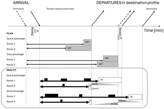
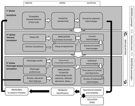
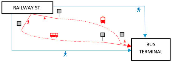
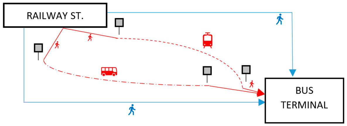
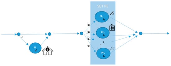
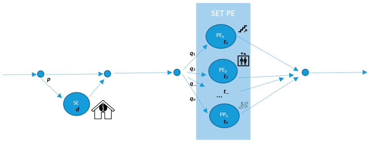
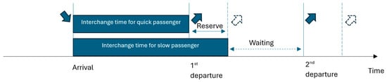
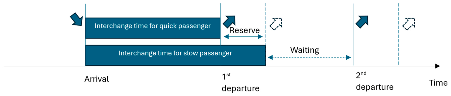
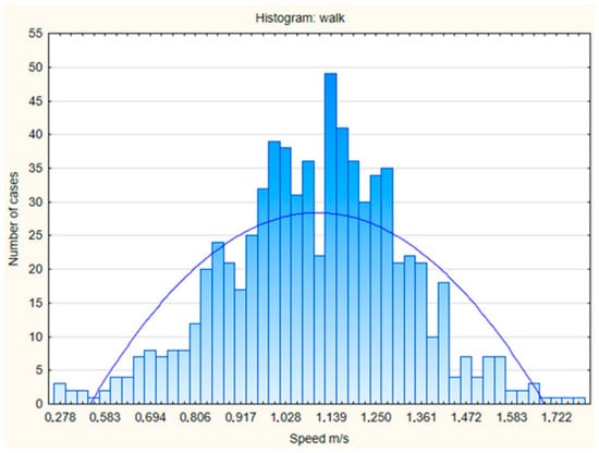
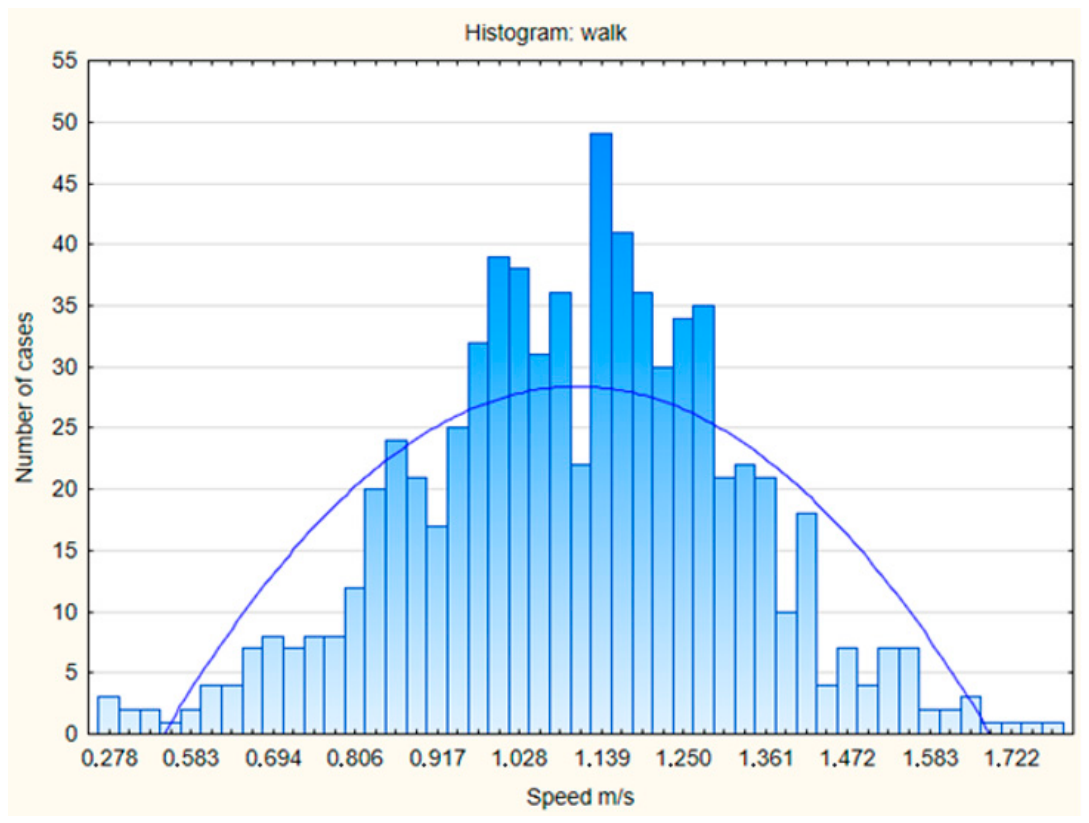
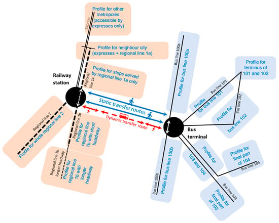
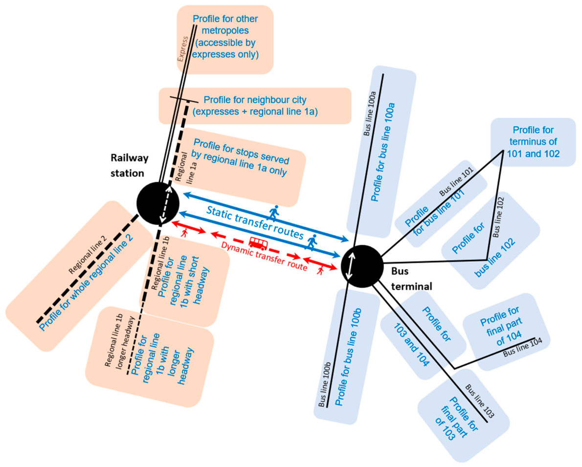
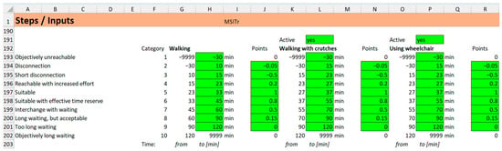
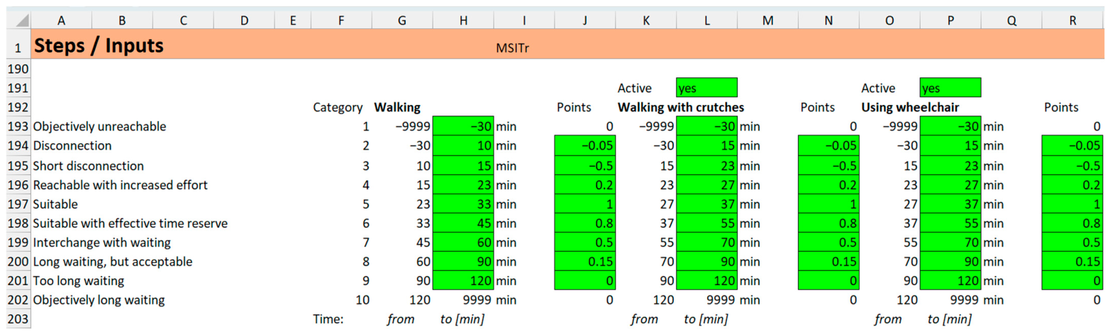
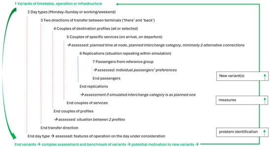
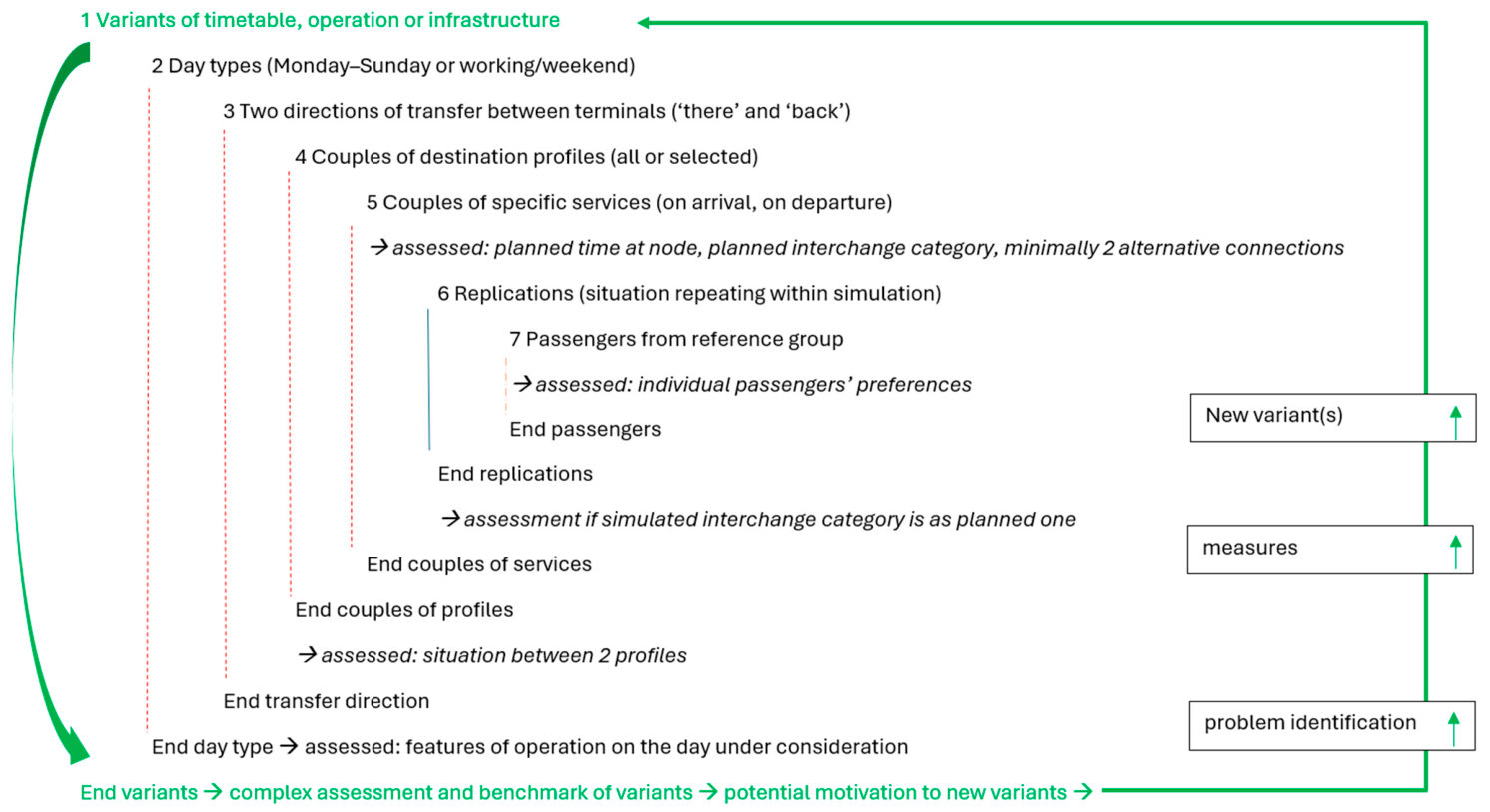
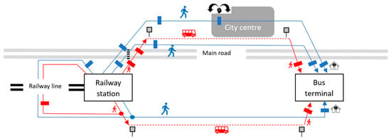
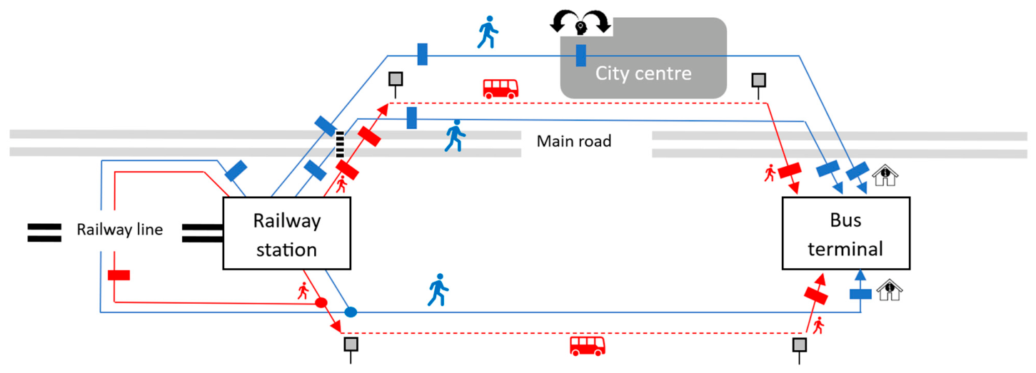
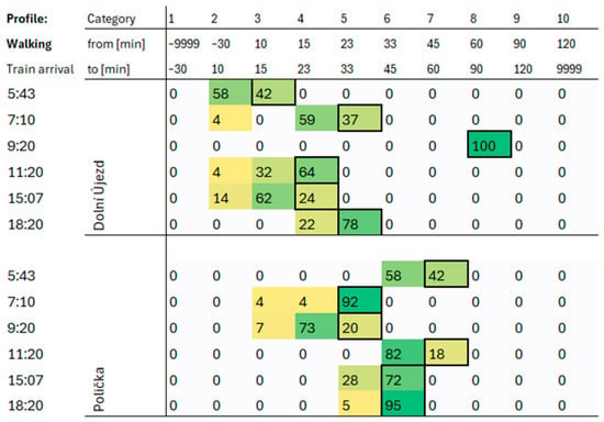
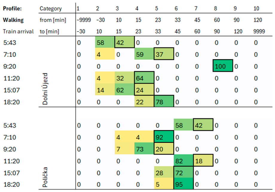
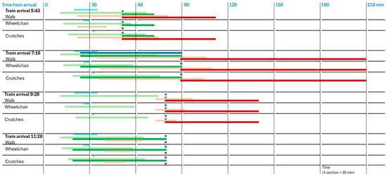
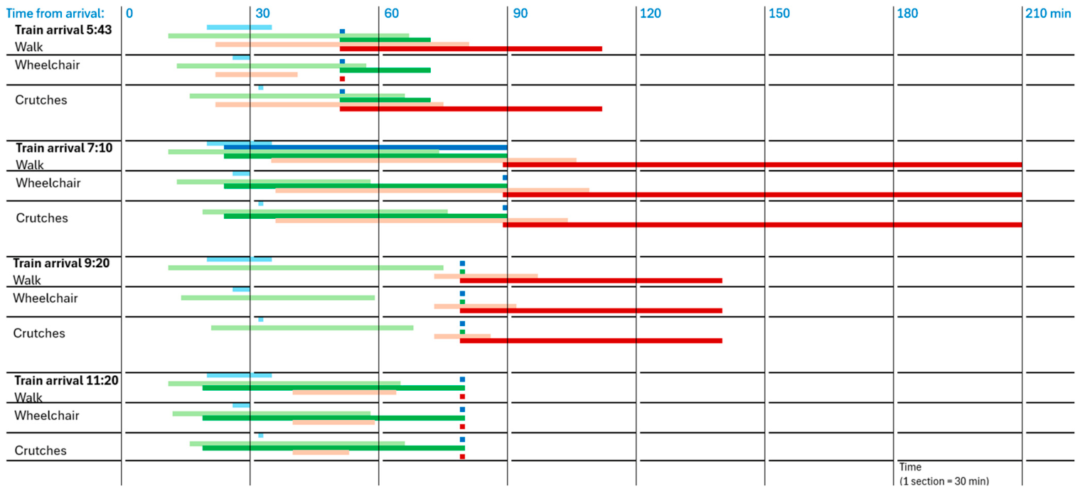
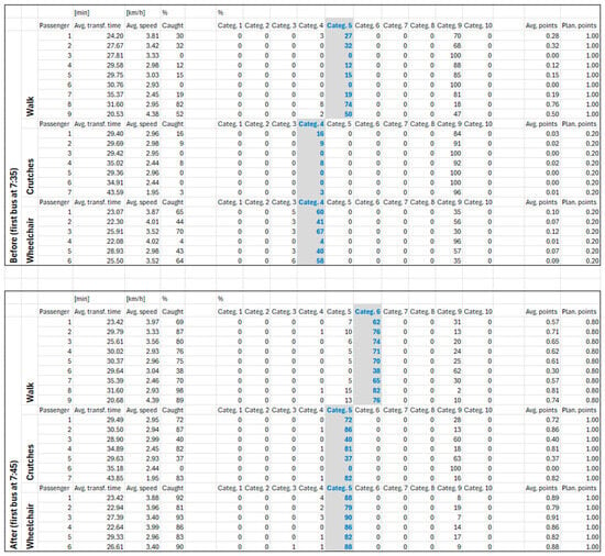
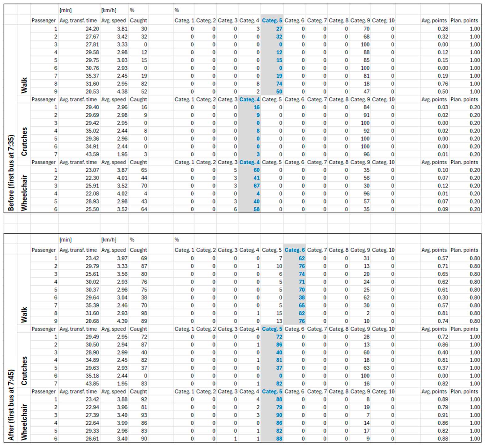
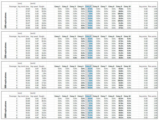
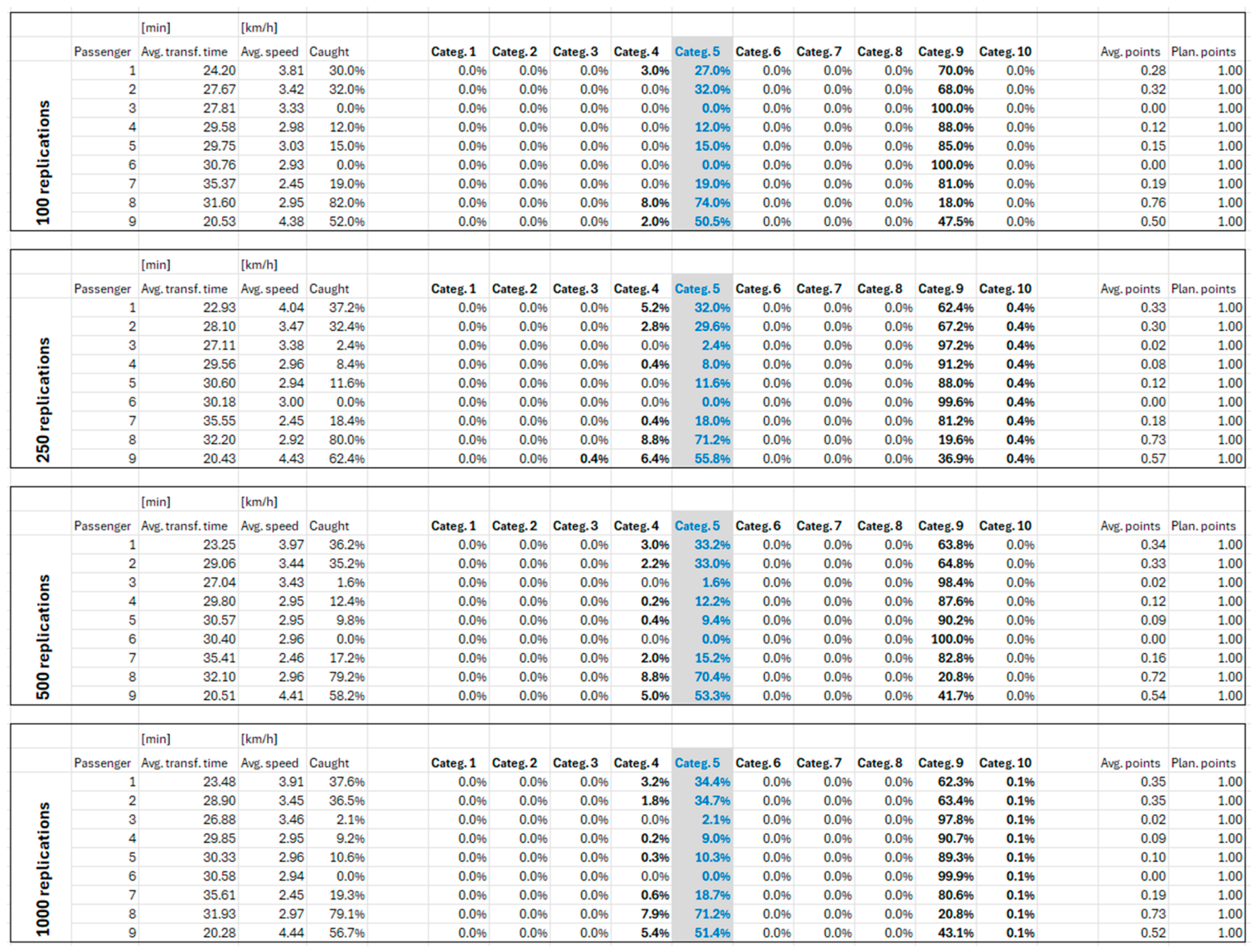

Disclaimer/Publisher’s Note: The statements, opinions and data contained in all publications are solely those of the individual author(s) and contributor(s) and not of MDPI and/or the editor(s). MDPI and/or the editor(s) disclaim responsibility for any injury to people or property resulting from any ideas, methods, instructions or products referred to in the content. |
© 2026 by the authors. Licensee MDPI, Basel, Switzerland. This article is an open access article distributed under the terms and conditions of the Creative Commons Attribution (CC BY) license.