


Abstract
Because power grids require real-time generation-load balance, enhancing Short-Term Load Forecasting (STLF) accuracy prevents frequency instability, optimizes unit commitment, and reduces carbon-intensive spinning reserve dispatch, thereby facilitating intermittent renewable energy integration. This study evaluates seven dimensionality reduction techniques (PCA, KPCA, UMAP, RF, XGBoost, AE, and VAE) integrated offline into the Spanish Transmission System Operator’s forecasting architecture. A 169-variable historical demand dataset is incorporated and compressed to feed three modeling paradigms: a linear autoregressive model, an ensemble of 10 nonlinear autoregressive neural networks, and their dynamically weighted hybrid combination. Results show that incorporating these new variables lowers the baseline Normalized Root Mean Squared Error (NRMSE) from 2.38% to 2.17%. Ultimately, compressing the input space to 20–21 variables achieves a 2.16% NRMSE, matching the full variable set. Scaling this accuracy gain to the Spanish grid’s mean load lowers the thermal backup requirement by roughly 198 MW, equivalent to a standard open-cycle gas turbine unit, reducing operational costs and carbon emissions. Finally, dimensionality reduction halves linear model training time while maintaining millisecond inference latency.
1. Introduction
The main operational constraint of utility-scale power systems lies in the limited capacity for energy storage. Consequently, the stability of national grids relies on maintaining a strict, real-time equilibrium between generation and consumption. Hence, accurate load forecasting becomes essential for operational planning. The absence of reliable future load estimates exposes the grid to severe risks, including frequency deviations and voltage instability, which endangers the continuity of supply.
Load forecasting methodologies are typically categorized by their temporal horizon: Long Term (spanning months to years), Medium Term (weeks), Short Term (hours to days), and Very Short Term (seconds to minutes). This research focuses specifically on Short-Term Load Forecasting (STLF), utilizing a predictive framework that operates within hours. This horizon is fundamental for grid operators, as it dictates unit commitment strategies and facilitates the optimization of maintenance schedules.
By minimizing forecasting errors, grid operators can reduce the safety margins required for costly spinning reserves and fast-ramping backup generation needed to buffer unexpected demand surges or prediction deviations. From an environmental standpoint, this accuracy improvement supports power sector decarbonization. Because balancing reserves and peaking units are predominantly supplied by dispatchable fossil-fuel thermal plants, operating them on standby or ramping them abruptly to cover forecasting errors results in suboptimal thermal efficiency and elevated specific greenhouse gas emissions. Furthermore, tighter demand prediction intervals reduce net-load uncertainty, which minimizes conservative security constraints and avoids the preventive curtailment of intermittent renewable energy sources such as wind and solar photovoltaics. Consequently, refining STLF techniques not only rationalizes operational and market costs, but also acts as a key enabling technology for lowering carbon intensity.
By projecting time-series data with high dimensionality onto a compact, representative feature subspace, dimensionality reduction techniques decouple the signal from noise. This compression of input information forces the model to internalize generic relationships rather than memorizing training data, ensuring robust generalization in novel operational scenarios.
1.1. State of the Art
1.1.1. Development of Forecasting Models
The field of load forecasting has a large number of published models. A large part of the published works is based on statistical models, i.e., algorithms with interpretable coefficients.
Hermias, J.P. [1] et al. utilize a Hidden Markov Model (HMM) with Gaussian emission probabilities to perform STLF. Lisi, F. et al. [2] investigate a Functional AutoRegressive model and its nonparametric counterpart for 1-day-ahead forecasting of electricity demand and prices. Mi, J. et al. [3] propose a multivariable grey model that incorporates first exponential smoothing to capture data trends effectively. Ji, P. et al. [4] develop an exponential smoothing model by optimizing the selection of the smoothing coefficient.
Wei, L. et al. [5] explore the application of Autoregressive Integrated Moving Average (ARIMA), addressing the limitations of traditional time series methods. Royal, E. et al. [6] present a Generalized Additive Model (GAM) combined with Seasonal ARIMA (SARIMA) for long-horizon hourly load. Owusu, F.K. et al. [7] propose a seemingly unrelated series (SUR) model combined with Kalman and Monte Carlo filtering to predict peaks in electricity demand.
Other models are based on machine learning, which has received more attention over time, since this kind of model captures nonlinear and temporal dependencies in complex datasets [8]. Mpawenimana, I. et al. [9] demonstrate greater accuracy of Long Short-Term Memory (LSTM) model over an ARIMA. Amasyali, K. et al. [10] assert that neural networks and Support Vector Machines (SVMs), in many cases, have better accuracy than decision trees and statistical methods for forecasting demand in buildings.
Demir, E. et al. [8] introduce a LSTM network combined with a Convolutional Neural Network (CNN) that integrates meteorological features like temperature and wind speed.
Alhussein, M. et al. [11] propose a CNN-LSTM framework for residential households up to 3 h ahead, using CNN layers for feature extraction and LSTM layers for sequence learning. Li, X. et al. [12] introduce a model with Kalman filtering to eliminate noise and Empirical Mode Decomposition (EMD) to break down the demand series, ultimately feeding into an SVM. Lenk, A. et al. [13] employ a Temporal Fusion Transformer (TFT) model for weekly energy demand forecasting. Tian, Z. et al. [14] propose a probabilistic deep learning framework that combines multi-layer CNNs with a Transformer architecture to generate day-ahead forecasts. Sun, C. et al. [15] propose a framework that integrates Graph Neural Networks (GNN) with dilated 1D-CNNs.
Hung, Y.-C. et al. [16] combine Gate Recurrent Units (GRU), self-attention, and Transformer mechanisms to forecast peak power load. Ferreira, A.B.A. et al. [17] utilize TFT, which allows the model to identify the most relevant variables and temporal patterns. Imani, M. [18] proposes a CNN to extract nonlinear spatial-temporal features from historical data, which are subsequently fed into a Support Vector Regression (SVR) model. Singh, P. et al. [19] integrate an Artificial Neural Network (ANN) with an evolutionary algorithm to avoid local optima and achieve convergence. Kamalov, F. et al. [20] introduce a Neural Basis Expansion Analysis for Time Series (N-BEATS) model on a massive, diverse dataset and then apply it directly to medium-term power generation.
There are also hybrid prediction systems that combine artificial intelligence with statistical techniques. These types of models have also received a lot of attention. Huang Z. et al. [21] obtain better results by combining statistical and machine learning techniques than with pure models separately. Makridakis, S. et al. [22] analyze the results of the M4 Forecasting Competition and conclude that combining statistical and/or machine learning models generates better results than isolated models.
Karthika, S. et al. [23] present an ARIMA model that generates a baseline prediction from the corrected historical data, while an SVM is subsequently used to model the residuals and refine the forecast. Rafi, S.H. et al. [24] develop a Convolutional LSTM, integrating convolutional operations within the LSTM architecture to capture complex spatiotemporal features. Su, Z. et al. [25] employ the Hodrick–Prescott (HP) filter to decompose time series, subsequently applying ARIMA to forecast the trend component and Recurrent Neural Networks (RNNs) to handle the periodic component. Liu, F. et al. [26] combine Improved Fuzzy C-Means (IFCM) to resolve uneven data distributions, Random Forest (RF) to handle features, and Deep Neural Networks (DNN) for the final prediction.
Sulandari, W. et al. [27] use Exponential Smoothing with the Holt–Winters method to decompose the time series, which are subsequently fed into a neural network. Pooniwala, N. et al. [28] merge Seasonal ARIMA (SARIMAX) with LSTM networks. Tarmanini, C. et al. [29] evaluate and contrast ARIMA with ANNs, revealing that the ANN offers better results than ARIMA. Mochurad, L. et al. [30] combine Temporal Convolutional Networks (TCN) to capture long-range temporal dependencies with Quasi-Recurrent Neural Networks (QRNN).
1.1.2. Dimensionality Reduction Applied to Load Forecasting
From a strict perspective in machine learning, the algorithms utilized in this study fall into two distinct categories: feature extraction (such as PCA, KPCA, UMAP, AE, and VAE that project data into a different space) and feature selection (such as RF and XGBoost that filter original variables without transforming the space). However, since both approaches serve the same purpose in this study (reducing the number of input variables to mitigate high dimensionality), they will be referred to collectively under the general term “dimensionality reduction” throughout this manuscript for simplicity.
The field of dimensionality reduction does not receive as much attention as the core predictive algorithms (such as ARIMA or LSTM networks), but there are previous studies in indexed journals. Some of the most commonly used techniques are explained in the following sections.
Principal Component Analysis (PCA) [31] is a linear transformation that converts a set of correlated variables into a new set of orthogonal variables (principal components), ordered according to the amount of original variance they explain. Mathematically, PCA seeks the eigenvectors of the data covariance matrix, projecting the original space onto these axes to minimize information loss (reconstruction error). This allows for the reduction of noise and redundancy, operating under the assumption that the most important features are statistically those with the highest variance.
PCA remains as benchmark in the energy sector, especially for linear models. Bianchi, F.M. et al. [32] successfully employed PCA to summarize daily loads and use the reduced features as input for Echo State Networks. Gordillo-Orquera, R. et al. [33] use PCA to analyze consumption patterns in healthcare buildings, demonstrating its utility in filtering noise from complex load profiles.
Saeedi, N. et al. [34] use PCA as a dimensionality reduction technique to reduce a 12-feature dataset into two and train an RF regressor and LSTM. Yi, L. et al. [35] use PCA to reduce 10 input variables to 5 and feed an LSTM network.
Kernel PCA (KPCA) [36] is a nonlinear extension of PCA; the procedure is the same with the only difference being the prior application of a kernel function to project the initial data into a higher dimensional space, then it can be linearly separated with PCA. This enables the extraction of complex, nonlinear structures (common in stochastic electricity demand) that traditional linear methods would overlook.
Fan, Y. et al. [37] applied KPCA combined with Kernel Extreme Learning Machines (KELM), while You, J. et al. [38] recently proposed a KPCA as part of preprocessing to feed an Extended LSTM (xLSTM) Informer architecture.
Uniform Manifold Approximation and Projection (UMAP) [39] is a nonlinear technique that operates under the assumption that data reside on a manifold. The process consists of two main stages. First, the algorithm analyzes the connectivity between points and their nearest neighbors in high-dimensional space to create a detailed topological representation. Subsequently, it optimizes the projection of this network into a lower dimensional space by minimizing the cross-entropy (discrepancy in connectivity) between the original and projected forms. This mathematical formulation enables a balance between preserving information from local structures and maintaining the overview of the global structure.
Yao, Y. et al. [40] apply UMAP to reduce the dimensionality of the input data composed of historical energy loads and meteorological data, and then feed a TCN-NBeats ensemble model to forecast electricity, cooling, and heating demands.
Bae, H.-J. et al. [41] compare KPCA and UMAP followed by k-means clustering to effectively manage high-dimensional household datasets. The use of KPCA and four clusters yields the best overall performance.
Autoencoders (AE) [42] are neural networks that learn to compress input data into a compact latent representation (encoder) and then reconstruct it (decoder), minimizing reconstruction error to retain significant features. Then, only the latent representation is used to infer. While they are effective for deterministic feature extraction, they often fail to capture the underlying probability distribution of volatile signals. Variational Autoencoders (VAE) [43] address this by mapping inputs to a probability distribution (characterized by mean and variance) instead of a fixed point in the latent space. This probabilistic constraint forces the model to organize the latent space such that similar input patterns are grouped together, preventing disjointed representations. By ensuring this continuity, the VAE filters out stochastic noise and produces a more generalized feature set.
Peng, S. et al. [44] compare AE with a PCA and a convolutional AE to predict consumption in Spain’s five largest cities, achieving better results with the traditional AE. Veeramsetty, V. et al. [45] use an autoencoder to transform 12 variables into 9 to train Radial Basis Function networks. Pajić, Z. et al. [46] use an AE to represent daily profiles in a reduced space, where they can be classified more effectively before training.
Moradzadeh, A. et al. [47] implemented VAEs to feed a bidirectional LSTM, effectively modeling the stochastic nature of demand. Yang, Y. et al. [48] employ variational mode decomposition; after that, VAE is applied to each sub-sequence to compress data for an LSTM network. Zeng, Q. et al. [49] utilize an AE reduction to feed a GRU architecture.
Unlike the previous techniques, XGBoost [50] and RF [51] do not perform dimensionality reduction by transforming the feature space, but rather by selecting the features most closely related to the target variable. XGBoost operates as a sequential boosting system, where successive trees are trained to specifically predict the residuals or errors of the preceding ones; within this iterative process, it measures the loss reduction achieved by specific variables at each split node. RF consists of an ensemble of independent decision trees built with random constraints (using both random subsets of data and a limited selection of variables at each node) to ensure diversity within the forest. It identifies influential variables by calculating the total decrease in node impurity.
Cui, J. et al. [52] employ a hybrid XGBoost-RF feature selection stage before feeding data into a CNN-GRU model, improving forecasting accuracy and execution speed.
Abbasimehr, H. et al. [53] use an XGBoost to filter meteorological and historical variables before feeding them into deep learning models. Mishra, K. et al. [54] use XGBoost as a forecasting engine and to distill datasets into a refined subset of features, increasing accuracy.
Xuan, Y. et al. [55] use RF to select the most relevant inputs for a predictive system based on Convolutional Neural Network and Bidirectional Gated Recurrent unit architectures. Deng, S. et al. [56] use an RF variation to classify different types of electrical load, thereby making the ensemble model independent of any single consumer type.
1.1.3. Literature Gap
Despite the advances reported in the reviewed literature, four methodological and operational gaps limit the direct transferability of existing dimensionality reduction studies to national-scale STLF.
First, previous works evaluate dimensionality reduction techniques in isolation or restrict their comparisons to a narrow subset of algorithms within the same methodological family. Specifically, several studies test a single reduction technique, such as PCA in Yi et al. [35], KPCA in Fan et al. [37] and You et al. [38], or compare only a few projection methods against each other, such as PCA versus Orthonormal Partial Least Squares (OPLS) in Gordillo-Orquera et al. [33]. Conversely, works applying tree-based feature selection, such as the hybrid XGBoost-RF approach in Cui et al. [52], do not benchmark their selected variable subsets against latent representations extracted by linear, kernel, manifold, or neural autoencoder techniques. Consequently, the literature lacks a unified benchmark that systematically contrasts feature extraction (PCA, KPCA, UMAP, AE, and VAE) and feature selection (RF and XGBoost) over the same high-dimensional historical load input space.
Second, existing studies predominantly couple dimensionality reduction with a single type of forecasting engine, most notably standalone deep learning or kernel architectures such as LSTM [35], Bidirectional Long Short-Term Memory (BiLSTM) [47], or ANN [46]. Even when multiple individual models are tested independently, as in Bae et al. [41], or when two deep learning architectures (TCN and N-BEATS) are fused in Yao et al. [40], the literature does not evaluate how each dimensionality reduction family interacts simultaneously with a linear autoregressive model, a nonlinear neural network ensemble, and their combined hybrid system. Furthermore, none of the reviewed autoencoder studies examine through an ablation analysis whether post-processing the nonlinear latent space of deterministic and variational autoencoders via PCA orthogonalization improves numerical conditioning and forecasting accuracy across linear and neural predictors.
Third, in the reviewed works, the configuration of the dimensionality reduction stage is largely decoupled from the final forecasting error, relying instead on intermediate statistical heuristics or fixed parameters. Specifically, Gordillo-Orquera et al. [33], Yi et al. [35], Fan et al. [37], You et al. [38], and Peng et al. [44] determine the retained components in PCA, KPCA, or AE using cumulative explained variance thresholds or contribution rates, whereas Saeedi et al. [34], Yao et al. [40], Bae et al. [41], and Pajić et al. [46] predefine a fixed number of target dimensions. Similarly, Veeramsetty et al. [45] optimize the AE architecture based on input reconstruction loss and variance deviation rather than downstream load prediction error, and Cui et al. [52] filter features using a static importance threshold of 0.01. Although Abbasimehr et al. [53] tune the number of XGBoost features and learning rate via Bayesian optimization, a systematic grid search that optimizes both the target dimensionality and the internal hyperparameters of all reduction methods directly against the downstream hybrid forecasting error has not been conducted.
Fourth, the majority of the reviewed studies validate dimensionality reduction at localized or disaggregated scales, including individual healthcare or green buildings and university campuses [33,34,40,49], distributed energy systems and 33/11 kV substations [37,45,56], household clusters [41], or city-level grids [48]. Although national or regional datasets are utilized in Yi et al. [35], You et al. [38], or Mishra et al. [54], these works evaluate standalone academic models or day-selection tools rather than integrating automated dimensionality reduction into a TSO forecasting engine.
1.2. Contributions
To address the gaps identified in the literature, this study conducts an evaluation of seven dimensionality reduction techniques; spanning linear extraction (PCA), nonlinear kernel and manifold mappings (KPCA and UMAP), neural autoencoders (AE and VAE), and tree-based feature selectors (RF and XGBoost), integrated into an industrial national-scale STLF framework. The main contributions of this paper are threefold.
1.2.1. Empirical Evaluation on a Validated National TSO Predictive Engine
Unlike studies restricted to standalone academic models or localized facilities, this work integrates dimensionality reduction offline into the operational forecasting architecture developed by López et al. [57] for the Spanish Transmission System Operator (TSO), Red Eléctrica de España (REE). Specifically, the original expert-engineered input space is expanded with a 7-day hourly demand window (forming a 169-variable historical load set to be reduced), and the resulting compressed representations are benchmarked at a national scale against both the original TSO baseline and the unreduced 169-variable configuration, using ten years of historical data.
1.2.2. Cross-Paradigm Analysis
This study evaluates how feature extraction and feature selection techniques interact across three distinct modeling paradigms within the same framework: linear (autoregressive model with errors and exogenous inputs, AR), nonlinear (an ensemble of 10 NARX neural networks), and hybrid (their dynamically weighted linear combination). Furthermore, rather than relying on intermediate variance thresholds or reconstruction losses, a grid search tunes both the target dimensionality and the internal hyperparameters of each reduction method directly against the downstream hybrid forecasting error.
1.2.3. Automated Scalability and Stage-Wise Computational Efficiency
This work provides a stage-wise computational time breakdown, demonstrating that dimensionality reduction cuts linear model training time by more than half compared to using all variables while maintaining inference latency within milliseconds for real-time TSO operation.
2. Materials and Methods
2.1. Forecasting Models
The predictive system used as a benchmark in this work is the one developed by López, M. et al. [57] for the Spanish Transmission System Operator (TSO), Red Eléctrica de España (REE). This architecture has been utilized at a national and regional scale for over a decade, establishing it as a highly representative baseline for offline experimentation.
The forecasting system consists of a combination of two main forecasting models: an autoregressive (AR) model with errors and exogenous inputs, and a nonlinear autoregressive neural network (NARX). Both models use the same exogenous inputs. To mitigate the intrinsic randomness of neural networks, the system employs a redundancy architecture with 10 averaged NARX networks after discarding extreme values. Once the AR and NARX model predictions have been obtained, both predictions are integrated through a linear combination based on the error over the last 30 days. This structure generates hourly curves for the national total using specific models pre-trained according to the time of issuance and the forecast horizon, which ranges from the current day to nine days ahead.
The AR model can be summarized by (1).
where yt is the natural logarithm of actual electricity demand at time t, α is the vector containing the autoregressive coefficients, p is the time series of prediction errors made by the AR model itself in the past, Ω is the vector of exogenous coefficients, Ht is the vector of exogenous inputs for predicting time t, ε is the time series of errors, and n is the number of previous errors taken into account (set to 7).
Each neural network takes exogenous variables as input, in addition to the 14 previous values that the network itself has obtained. During training, the 14 predicted previous values are not available, so training is performed in an open-loop configuration using only actual values as input. For inference, the loop is closed by replacing the actual values with the previous values that the network itself has obtained.
To make daily forecasts, the system uses temperature data from five weather stations (Sevilla, Madrid, Barcelona, Zaragoza, and Bilbao), calculating the daily average temperature for each station and then deriving the heating degree days (HDD) and cooling degree days (CDD). The system also uses the type of day as an input; to this end, it describes each day using 54 variables that have been meticulously designed based on expert criteria.
For this study, a new set of variables has been implemented consisting of the hourly demand for the previous 7 days, that is, 168 variables. Dimensionality reduction is applied to this set along with the average demand over the last 365 days (a variable already present in the original system), resulting in 169 variables to be reduced. These new variables are the only ones that will undergo dimensionality reduction, leaving the rest of the variables unchanged.
2.2. Hyperparameter Tuning
The hyperparameters of the dimensionality reduction techniques were optimized using a grid search, with the hybrid model’s prediction error serving as the objective function to be minimized. This approach ensures that the transformation of the input space is directly aligned with the system’s accuracy, avoiding the loss of relevant information that occurs when using intermediate metrics that assume a direct correlation with accuracy (such as explained variance).
To ensure the optimization process aligns with operation requirements, the grid search was conducted on the integrated hybrid model (combining linear and NARX components), as this is the primary forecasting engine utilized by the TSO.
Since each dimensionality reduction technique has a different hyperparameter structure, a set of diverse candidate values was defined for each one. Optimization was performed using a grid search, evaluating all possible combinations of these values.
The time range covered by this study consists of the remaining hours of the day after temperature data are received (8 a.m.), that is, intraday forecasts starting at 9 a.m. Since each forecast hour has an AR model and 10 NARX networks, applying the grid search to all 15 models would multiply the number of trainings by 15. To make this feasible, the grid search was applied to one of the most difficult hours to predict, from 8:00 to 9:00 p.m., and the configuration obtained was then applied to the remaining hours.
In electricity load forecasting, the operational and economic impact of an error does not follow a linear progression; it is more similar to a quadratic one. A single large error is considerably more critical to grid stability than multiple small errors. This asymmetry is captured by the Root Mean Squared Error (RMSE); by squaring the deviations, the metric gives greater weight to outliers. Thus, between two models with the same mean absolute error, the RMSE will penalize the one whose forecasts deviate significantly at few moments, better reflecting the system’s actual risk.
In this study, the RMSE employed is expressed as the percentage of the mean actual demand, that is the Normalized Root Mean Squared Error (NRMSE); see (2). Unlike RMSE, NRMSE facilitates the comparison of forecasting performance across different scales of demand or between disparate power grids. This metric has been used as an objective function to be minimized in the grid search for hyperparameter tuning, as well as a measure of error in the final experiments, where dimensionality reduction is applied to the test dataset to prevent bias.
where r is the time series of actual demand values, f is the time series of forecasted demand values and N is the number of available samples.
The hyperparameter values selected for each technique are as follows:
2.2.1. PCA
- Number of dimensions: 1, 2, 3, 4, 5, 6, 8, 10, 12, 16, 20, 26, 33, 41, 52, 66, 83, 106, 133, or 169 (20 values with logarithmic spacing).
2.2.2. KPCA
In the case of KPCA, each iteration of the grid search can vary between 7 dimension numbers and 3 kernel functions: simple radial basis function, scaled radial basis function, and polynomial kernel. The polynomial kernel is tuned using 3 hyperparameters, so all combinations of these hyperparameters (18) are added to the combinatorial set, resulting in a total of 140 configurations (7 dimensions multiplied by 20 different kernel functions).
- Number of dimensions: 1, 2, 7, 20, 21, 60, or 169 (6 values with logarithmic spacing and the best number from PCA).
- Kernel function: it measures similarity between two input vectors. It can be one of the following options:
- Simple radial basis function: defined in (3).
- Scale radial basis function: defined in (4).
- Polynomial kernel: defined in (5). This kernel can have all the following options for each parameter:
- Polynomial degree: 2 or 3
- Independent term: 0, 1, or 5
- Scaling factor: 0.1, 1, or 10
2.2.3. UMAP
- Number of dimensions: 1, 2, 7, 21, 60, or 169 (6 values with logarithmic spacing).
- Number of neighbors: it defines the size of the local neighborhood that UMAP examines to learn the topology of the data; it can be set to 5, 11, 27, 64, or 150.
- Minimum distance: minimum allowed distance between points in the low-dimensional representation; the larger this value is, the more widely dispersed the data points are in the final space. It can be 0, 0.1, 0.25, 0.5, 0.75, or 0.99.
2.2.4. AE
- Number of dimensions: 1, 2, 7, 21, 60, or 169 (6 values with logarithmic spacing).
- Learning rate: it adjusts the step size of the training algorithm (Adam) toward the minimum of the loss function at each iteration. It can be set to 10−2, 5 × 10⁻³, or 10−3.
- L2 Penalty: it prevents overfitting by adding a penalty to the neuron weights. It can be set to 0, 10−4, or 10−5.
- Batch size: it divides the dataset into subgroups during training; larger values make training more stable and computationally faster, but can lead to poorer generalization. It can be set to 16, 32, or 64.
2.2.5. VAE
- Number of dimensions: 1, 2, 7, 21, 60, or 169 (6 values with logarithmic spacing).
- Batch size: 16, 32, or 64.
- KL weight: it allows the distribution of the latent space to resemble a normal distribution, so that higher values increase the final similarity between input vectors after they are mapped to the compressed space. It can be set to 0.1, 1, or 5.
- Learning rate: it can be set to 10−2, 5 × 10⁻³ or 10−3.
- L2 Penalty: it can be set to 0, 10−4, or 10−5.
2.2.6. RF
- Number of dimensions: 1, 2, 7, 21, 60, or 169 (6 values with logarithmic spacing).
- Maximum depth: limit of number of branches a tree can have from the root to the outermost leaf. It can be set to 10, 15, 25, or unlimited.
- Minimum samples per leaf: each node will only become a leaf if it contains at least this number of samples. It can be 1, 3, 5, or 10.
- Maximum features: how many variables are randomly selected to find the best cut at each node. This can be the square root of the number of available features, or all of them.
2.2.7. XGBoost
- Number of dimensions: 1, 2, 7, 21, 60, or 169 (6 values with logarithmic spacing).
- Maximum depth: it can be 3, 6, or 9.
- Learning rate: factor that reduces the contribution of each new tree; a low value makes learning slower and more conservative. It can be set to 10−1, 10−2, or 5 × 10⁻².
- Minimum child weight: it controls the minimum number of samples required for the tree to create a new branch. It can be set to 1, 3, or 5.
2.3. Variable Handling and Consistency of Feature Space
Before applying PCA, the demand variables were standardized so that each had a mean of zero and a variance of one, thereby ensuring that PCA identifies correlation patterns without being biased by differences in data dispersion. Similarly, before applying KPCA, the same type of standardization was also applied to ensure that the kernel distance calculation does not ignore variables with smaller ranges.
Prior to UMAP, standardization was applied to ensure that distance calculations in high-dimensional space are fair, allowing the algorithm to accurately capture the topological structure and neighborhood relationships of the demand without biases arising from different dispersion scales.
For AE and VAE, the hyperbolic tangent was used as the activation function; therefore, a Min–Max scaling was previously applied to normalize the variables within the dynamic range between −1 and 1, ensuring that the input data fall within the function’s most sensitive range to avoid gradient saturation.
Following feature extraction using AE and VAE, standardization was applied, followed by PCA without dimensionality reduction to orthogonalize the latent space. Orthogonalization ensures that the coefficients of the linear model are numerically stable and represent the independent contribution of each component. Furthermore, for neural networks, the input of decorrelated data improves the conditioning of the optimization problem. By providing an orthogonal basis, the risk of multiple neurons learning redundant patterns is reduced, facilitating faster and more stable convergence.
To justify the necessity of this orthogonalization step, an ablation analysis was incorporated into the experimental design. The performance of both AE and VAE was evaluated and reported twice: applying the PCA post-processing, and without it. This allows for a direct assessment of how decorrelating the latent space impacts the stability and accuracy of the subsequent predictive models.
No prior scaling or standardization was applied to the RF and XGBoost models, as decision tree-based algorithms are scale invariant. By performing recursive partitions of the feature space using thresholds, these models rely on the order of magnitude of the data rather than on Euclidean distances, making them inherently robust to variables with different ranges and distributions.
2.4. Dataset Descriptions
National demand data were obtained for each hour using the REData API [58], provided by REE. The temperature records were obtained using the OpenData API [59] from Spain’s national meteorological agency (AEMET).
Demand data are recorded hourly, while temperature data are recorded daily. For each day, the temperature used is the average of the maximum and minimum temperatures. Therefore, for each year, there are 365 temperature values (366 temperature values in leap years).
The temporal data were partitioned into different subsets to ensure a robust evaluation of preprocessing techniques. For the hyperparameter tuning phase, a training set of ten years from 2013 to 2022, both included, was used to fit the models to forecast the load from 8 p.m. to 9 p.m. The year 2023 served as a validation set to select the optimal configuration from the grid search based on the NRMSE.
Once the best parameters were identified for each preprocessing method, each preprocessing method had its forecasting models (AR and NARX) trained for the hours of the rest of the day (from 9 a.m. until midnight). A sliding window approach was implemented: the training window was shifted forward to cover the 2014–2023 period. Finally, each preprocessing model system was evaluated on the test set of 2024, providing an unbiased assessment of the system’s performance on unseen future data.
Regarding data integrity, no imputation was required as the TSO and meteorological APIs provided complete historical series. Furthermore, it is important to emphasize that data from the year 2020 were deliberately included in the training sets without any artificial smoothing, dummy variables, or special treatment for the COVID-19 lockdown anomalies. Retaining these severe load disruptions serves to validate the robust generalization capabilities of the forecasting architecture, demonstrating its resilience against extreme and unforeseen exogenous shocks without relying on manual data manipulation.
2.5. Experimental Procedure
The experimental procedure is summarized below, delineating the sequential stages for each dimensionality reduction method.
- Grid search initialization: define candidate hyperparameter combinations.
- Training phase: fit the models within each configuration using the historical dataset from 2013 to 2022. All preprocessing scalers (e.g., mean, variance, min, max) and dimensionality reduction mappings (e.g., PCA eigenvectors, AE/VAE weights) were fitted using this dataset (2013 to 2022).
- Validation: generate hourly forecasts for the year 2023 and calculate the resulting NRMSE for every configuration. This step includes the Diebold–Mariano test for Table 2.
- Optimization: identify and select the hyperparameter combination that yields the lowest NRMSE.
- Model retraining: retraining the models with data from 2014 to 2023. Again, all preprocessing scalers and dimensionality reduction mappings were fitted using this dataset (2014 to 2023).
- Final evaluation: perform inference on the unseen 2024 test set to obtain an unbiased assessment of the system’s performance.
- Statistical analysis: compare performance across paradigms using the NRMSE and the Diebold–Mariano test [60]. Given that the system predicts the remaining 15 h of the day simultaneously (from 9:00 a.m. to midnight), the forecast errors exhibit a moving average structure due to serial autocorrelation. To account for this dependence and prevent the underestimation of the long-run variance, the Diebold–Mariano statistics were computed using a forecast horizon of 15 alongside the Bartlett estimator. By applying linearly decaying weights to the sample autocovariances, this estimator guarantees a positive variance.
In addition, each training and inference follows the following sequence of steps for the 169 variables to be reduced:
- Preprocessing: standardization with mean zero and variance one for PCA, KPCA, and UMAP. Min–Max scaling for AE and VAE.
- Dimensionality reduction.
- Postprocessing: PCA without dimensionality reduction.
- Use of reduced variables: forecast future load or fit AR and NARX models.
2.6. Experimental Setup
For executing forecasts, data availability at 9:00 a.m. was simulated to predict the hourly loads between 9:00 a.m. and midnight on the same day.
The experimental procedure was implemented in Windows 11 Pro, with Python 3.11 using standard data science libraries: Numpy 2.3.4, Pandas 2.3.3, Scikit-learn 1.8.0, Umap 0.5.11, XGBRegressor from Xgboost 3.2.0, PyTorch 2.10.0, Statsmodels 0.14.6, and Matplotlib 3.10.7.
The computer employed has an Intel 13th Generation i7 CPU and 16 GB of RAM DDR5.
2.7. Implementation Details for Reproducibility
2.7.1. NARX Configuration
The NARX forecasting ensemble was implemented in Python 3.11 using the PyTorch 2.10.0 (torch.nn and torch.optim) and Scikit-learn 1.8.0 (StandardScaler) libraries. For each intraday target hour (from 9:00 to 23:00), an independent ensemble of 10 feedforward multi-layer perceptron networks with exogenous inputs and autoregressive feedback was trained. Each network comprises three layers: an input layer of size 110 + d (where d is the number of historical demand features retained), a single fully connected hidden layer with 15 neurons using a hyperbolic tangent activation function, and a fully connected linear output layer with a single neuron. Prior to training, the weight matrices of both the hidden and output layers are initialized via the Xavier (Glorot) uniform distribution (xavier_uniform), while all bias vectors are initialized to zero to prevent early gradient saturation within the hyperbolic tangent active region.
For each target hour, the input vector fed into each NARX network is structured into three distinct blocks:
- Unscaled categorical calendar block (65 variables): It comprises 54 expert-defined day-type and holiday indicators alongside 11 binary dummy variables encoding the month of the year (February through December, with January as the reference baseline).
- Fixed continuous block (45 variables): consists of
- ○
- 14 daily autoregressive feedback lags representing the natural logarithm of the demand at the same target hour over the previous 14 days
- ○
- 30 piecewise-linear thermal inputs corresponding to the Cooling Degree Days (CDD) and Heating Degree Days (HDD) derived from the daily mean temperatures (the mean is calculated from the maximum and minimum daily temperatures) across the five reference weather stations for the target day and the two preceding days (thermal lags 0, 1, and 2, with station-specific comfort thresholds optimized between 5 and 25 °C at a 0.1 °C resolution
- ○
- One immediate autoregressive input containing the natural logarithm of the last known hourly demand prior to forecast execution (i.e., at 08:00 a.m. for the 09:00 a.m. intraday run).
- Historical demand block (d variables): in the baseline configuration (original method), this block contains only d = 1 variable, namely the 365-day rolling mean of the log-demand at the target hour shifted by 7 days (yielding a total input layer size of 111 neurons). In the unreduced expansion (all variables), it incorporates the 168 hourly log-demands from the previous 7 complete calendar days plus the 365-day rolling mean, totaling d = 169 variables (279 input neurons). In the dimensionality reduction configurations, this 169-variable block is compressed into d latent or selected features.
A two-stage scaling pipeline is applied during preprocessing to preserve numerical conditioning. First, the 169-variable historical demand block is scaled according to the specific requirements of each dimensionality reduction operator (as detailed in Section 2.3) and projected onto the d-dimensional subspace. Second, the resulting d features are concatenated with the 45 fixed continuous variables, and the combined (45 + d)-dimensional continuous vector is standardized to zero mean and unit variance using a dedicated z-score scaler (StandardScaler), before being concatenated with the 65 unscaled categorical indicators. Similarly, the target output (hourly national load in MW) is transformed via the natural logarithm and standardized to zero mean and unit variance using an independent StandardScaler fitted exclusively on the training data.
Network training is carried out in an open-loop configuration by minimizing the Mean Squared Error (MSELoss) in the standardized logarithmic target space. To replicate the second-order convergence properties of the Levenberg–Marquardt algorithm used in the reference TSO architecture, each network is trained in full-batch mode using the Limited-memory Broyden–Fletcher–Goldfarb–Shanno (LBFGS) quasi-Newton optimizer with a learning rate of 0.1, a maximum of 500 iterations, and a curvature history size of 100. During inference, the predictions of the 10 networks are inverse transformed via the target scaler and exponentiated to recover values in MW. The 10 outputs are then sorted in ascending order, the highest and lowest extreme values are discarded, and the arithmetic mean of the 8 central predictions is computed as the final NARX forecast.
2.7.2. Variables Selected by RF and XGBoost
To reproduce the selections made by RF and XGBoost algorithms, Table 1 shows the variable selected for each algorithm and hour forecasted (since each forecasted hour requires a different training to create a dedicated model). The selected variables are denoted as D-x (hh:mm), where D represents the target forecasting day, x indicates the number of lag days (e.g., D-1 is the previous day), and (hh:mm) specifies the hour of the historical load. Mean_365d refers to the 365-day rolling mean of the target hour.
Table 1.
Variables selected by RF and XGBoost for each forecasted hour.
2.7.3. Other Details
To ensure reproducibility, the random seeds for the NumPy 2.3.4, TensorFlow 2.20.0, and Scikit-learn 1.8.0 libraries were uniformly fixed to 42 across all dimensionality reduction experiments. The neural architectures for both the AE and VAE were dynamically scaled based on the input dimension and the target number of latent components. The encoder and decoder were constructed with two symmetric hidden layers utilizing hyperbolic tangent activation functions, while the bottleneck and output layers employed linear activations. The neuron count was defined in (6) and (7).
where Nouter is the number of neurons at the outer hidden layer, Nhidden is the number of neurons at the inner hidden layer, F is the number of final dimensions, and I is the number of input dimensions.
During the training phase, both AE and VAE models were configured with a maximum of 150 epochs. To prevent overfitting, an early stopping mechanism monitored the loss function with a patience of 10 epochs, restoring the best model weights. For the feature selection phase, the XGBoost algorithm was initialized with a maximum of 3000 estimators and an early stopping criterion of 50 rounds. This was evaluated against a 20% validation split extracted sequentially, without chronological shuffling, to preserve the temporal integrity of the dataset.
3. Results
3.1. Error Improvement Due to Hyperparameter Tuning
The implementation of grid search for hyperparameter tuning allows us to assess whether the internal configuration of the reduction techniques influences the final accuracy, or whether the predictive models are capable of compensating for suboptimal configurations during their own training. To analyze this issue, Table 2 presents the best result obtained for each technique, as well as the worst result with the same number of dimensions. The metrics in Table 2 reflect exclusively the hyperparameter optimization phase, evaluated solely on the 2023 validation set for the single 20:00 forecasting hour.
Table 2.
Grid search results.
It also includes the p-value of the Diebold–Mariano test [60] to assess the statistical significance of the differences in predictive accuracy. The null hypothesis of the test assumes that the two competing forecasting models have equal expected predictive accuracy. Since the system’s performance is evaluated using the NRMSE, the test is conducted employing the squared-error loss function. Consequently, a p-value below the 0.05 significance level leads to the rejection of the null hypothesis, providing statistical evidence that the difference in forecasting accuracy between the evaluated configurations is significant at the 5% level.
The results in Table 2 show that the performance of dimensionality reduction techniques is sensitive to the configuration of their internal hyperparameters, beyond the selected number of dimensions.
Specifically, all p-values obtained from the Diebold–Mariano test when comparing the best and worst hyperparameter configurations (while keeping the optimal number of dimensions fixed) fall below the 0.05 significance threshold. This provides statistical evidence, at the 5% significance level, that a suboptimal configuration of the dimensionality reduction yields a significant degradation in forecasting accuracy, which the downstream AR and NARX models are unable to mitigate.
Furthermore, tree-based techniques achieve the lowest validation errors for the analyzed hour, led by RF with an NRMSE of 1.33% and followed closely by XGBoost at 1.34%, both selecting a subset of 21 variables.
Moreover, most algorithms converge toward a reduced subspace of similar dimensionality (20 dimensions for PCA and 21 dimensions for AE, VAE, RF, and XGBoost) whereas kernel-based and manifold techniques (KPCA and UMAP) concentrate their optimal configuration into a single dimension, recording minimum errors of 1.62% and 1.56%, respectively.
Finally, neural network-based reduction models (AE and VAE) exhibit the highest sensitivity to internal hyperparameter tuning for a fixed dimensionality; with NRMSE variations spanning from 1.54% to 1.86% in AE and from 1.61% to 2.04% in VAE without PCA. The PCA orthogonalization post-processing step yields virtually identical results for the best AE case (1.54%) and a slight improvement for VAE (1.60% with PCA versus 1.61% without PCA).
3.2. Performance of Forecasting Models
After tuning the hyperparameters, models were trained and predictions were made for hours from 9:00 a.m. to midnight for the year 2024. Unlike the isolated tuning phase presented in Table 2, the following results represent the final unbiased evaluation across all intraday forecasting periods. Figure 1 shows the NRMSE of the hybrid system for each preprocessing method. The “all variables” method uses all 169 previous demand variables, while the “original method” is derived from the original system and does not apply the new set of variables. Figure 2 and Figure 3 show the same metric for the autoregressive linear system and the neural network, respectively.
Figure 1.
NRMSE from each input preprocessing for the hybrid model.
Figure 2.
NRMSE from each input preprocessing for the AR model.
Figure 3.
NRMSE from each input preprocessing for the NARX model.
Figure 1, Figure 2 and Figure 3 reveal, first, that incorporating the new demand variables from the previous seven days (“all variables”) substantially reduces forecasting error compared to the baseline configuration (“original method”) across all three modeling paradigms evaluated over the year 2024. Specifically, when including the complete feature set, the NRMSE decreases from 2.38% to 2.17% in the hybrid model (Figure 1), from 2.58% to 2.16% in the linear AR model (Figure 2), and from 2.52% to 2.26% in the neural NARX model (Figure 3).
In the AR model (Figure 2), utilizing the full set of variables (“all variables”) provides the lowest NRMSE (2.16%), whereas any dimensionality reduction entails a loss of accuracy; among the reduction methods, the feature selectors RF (2.29%) and XGBoost (2.31%) preserve performance better than the rest.
Conversely, in the NARX model (Figure 3), reducing dimensionality improves accuracy regarding using all variables (2.26%): XGBoost lowers the NRMSE to 2.18%. When integrating both predictions into the hybrid model (Figure 1), PCA, XGBoost, and RF reach an NRMSE of 2.16%, matching “all variables” (2.17%) while relying on only 20 or 21 features.
Meanwhile, autoencoder-based feature extraction methods exhibit intermediate performance in the hybrid system, ranking slightly above “all variables” but clearly outperforming the original method in both AE (2.19%) and VAE (2.21% with PCA and 2.25% without PCA).
Regarding the ablation analysis on latent space orthogonalization, applying PCA without dimensionality reduction after VAE consistently improves accuracy across all three paradigms (reducing the NRMSE from 2.25% to 2.21% in the hybrid model, from 2.56% to 2.53% in AR, and from 2.39% to 2.35% in NARX), whereas in the deterministic AE, it produces no change in the hybrid (2.19%) and AR (2.54%) models, and slightly increases error in NARX (from 2.26% to 2.30%).
The nonlinear techniques KPCA and UMAP cause a severe degradation in forecasting performance across all models, yielding errors substantially higher than even the original system without the new demand variables.
To assess the error consistency, the p-value of the Diebold Mariano test was calculated, comparing each method with using all variables, resulting in Table 3.
Table 3.
The p-values obtained from the Diebold–Mariano test of final predictions.
The Diebold–Mariano test results reported in Table 3 evaluate the statistical significance of the observed accuracy differences relative to using the complete set of variables (“all variables”). First, the extremely low p-values corresponding to the “original method”, KPCA, and UMAP demonstrate that both the accuracy gain achieved by incorporating the new historical demand variables and the performance degradation caused by KPCA and UMAP are statistically significant across all three modeling paradigms.
Second, the column corresponding to the AR model shows p-values below 10−4 for every evaluated technique. This statistically confirms that the AR model exploits the information contained across all 169 original variables and that any compression or filtering of the input space induces a statistically significant loss of accuracy.
However, this behavior changes in the NARX model and the hybrid system. For PCA, XGBoost, RF, AE (with and without PCA), and VAE with PCA, the p-values substantially exceed the 0.05 significance threshold in both NARX and the hybrid model. From a statistical standpoint, this demonstrates that compressing the input space from 169 to 20–21 dimensions through these techniques yields forecasts whose accuracy is not statistically distinguishable from using all variables in both the hybrid engine and the NARX networks. Additionally, contrasting VAE without PCA against VAE with PCA in Table 3 validates the effectiveness of the orthogonalization step: whereas VAE without PCA exhibits a statistically significant degradation in NARX and a borderline effect in the hybrid model, applying PCA post-processing raises these p-values to 0.062 and 0.26, respectively.
To evaluate how each preprocessing method behaves under diverse operational regimes, Table 4 presents the NRMSE (%) obtained by the hybrid forecasting system across different day types (weekdays and weekends), meteorological seasons (winter and summer), and three representative intraday horizons (9:00, 16:00, and 23:00) during the 2024 test year.
Table 4.
NRMSE (%) of different contexts.
Comparing the dimensionality reduction algorithms against each other and against the “all variables” benchmark shows that XGBoost, RF, and PCA not only maintain their robustness across all scenarios, but actually outperform the full variable set in high-complexity contexts. Specifically, during both winter and summer, RF (2.60% and 1.59%), XGBoost (2.61% and 1.63%), and PCA (2.62% and 1.67%) reduce the NRMSE below the “all variables” baseline (2.72% and 1.71%). Likewise, XGBoost achieves the lowest NRMSE overall during both the highest-error hour (2.60% at 16:00) and the end of the day (1.34% at 23:00), whereas RF matches the global minimum at 9:00 (0.90%) and ties with XGBoost for the best performance on weekdays (2.11%) and weekends (2.29%).
Furthermore, all reduction techniques, with the exception of KPCA and UMAP, clearly outperform the original method on weekdays and weekends, in winter and summer, and at 9:00 and 16:00. Only at the 23:00 horizon does the original method (1.41%) match RF (1.41%) and improve upon PCA (1.49%), AE (1.50–1.52%), and VAE (1.52–1.59%), being surpassed at that hour solely by XGBoost (1.34%) and “all variables” (1.39%).
Complementing the quadratic error analysis, Table 5 reports the Mean Absolute Percentage Error (MAPE, in %) of the hybrid model across the same seasonal and intraday contexts, along with the global cumulative error (Total) over the entire evaluation period.
Table 5.
MAPE (%) of different contexts.
The MAPE evaluation reported in Table 5 corroborates the trends previously observed with the NRMSE in Table 4. Regarding overall performance (“Total”), the feature selection methods XGBoost and RF achieve the lowest cumulative error in the study with a total MAPE of 1.58%, slightly outperforming the complete variable set (1.60%) and markedly improving upon the original method (1.81%). Meanwhile, both PCA and AE (with and without PCA) register a total MAPE of 1.61%, performing at virtually the same accuracy level as the unreduced 169-variable configuration.
RF leads accuracy on weekdays (1.53%), weekends (1.71%, tied with XGBoost), and in summer (1.26%), whereas XGBoost achieves the best absolute results in winter (1.89%), at 16:00 (2.01%), and at 23:00 (1.04%). At the first forecasting hour (9:00), “all variables” reaches the lowest value (0.68%), followed closely by RF (0.70%) and AE without PCA (0.71%). Similarly, the strong relative performance of the original method at 23:00 (1.10%) is reproduced, tying with RF and slightly improving upon “all variables” (1.12%), while being outperformed only by XGBoost (1.04%). The MAPE results confirm the consistent benefit of applying PCA orthogonalization to VAE across all contexts, as well as the underperformance of KPCA and UMAP.
To assess the impact of dimensionality reduction on execution times, Table 6 has been compiled, showing the time required to train and run each AR and NARX model for different inputs. Table 6 also quantifies the time required to fit the transformation operators responsible for mapping the original feature vector X ∈ ℝ169 to the reduced latent subspace Z ∈ ℝd.
Table 6.
Computation times.
To ensure consistent measurements, the training process was timed only for the adjustment of the internal coefficients after the input data had been constructed and preprocessed. The time required to create the reduction operators (action performed before training the models) and the time needed to process the inputs they receive (action performed during inference) were also timed. Since XGBoost and RF are feature selection techniques, the operation simply involves extracting the columns of the input matrix.
According to the linear model, using the full set of variables results in the highest computational cost for training, requiring more than twice as much time as other methods; whereas dimensionality reduction allows training times to approach those of the original method. Unlike AR, the training and inference of NARX do not show significant variations in their times when the input type is changed.
PCA stands out as the most robust technique in terms of timing, with the shortest times for operator construction and application. Furthermore, the linear and NARX models maintain training and inference times similar to the original.
4. Discussion
4.1. Comparative Analysis
The experimental evaluation on data from the Spanish grid demonstrates that combining a recent load history with dimensionality reduction simultaneously optimizes forecasting accuracy and computational efficiency.
First, incorporating the hourly demand variables from the previous seven days significantly reduces forecasting error relative to the original expert baseline, lowering hybrid NRMSE from 2.38% to 2.17% and total MAPE from 1.81% to 1.60%.
Second, compressing this 169-variable set to 20 dimensions via PCA or 21 variables via RF and XGBoost yields a 2.16% hybrid NRMSE and a 1.58–1.61% MAPE, showing no statistically significant difference from using all variables while outperforming the unreduced set during winter, summer, and afternoon ramps (16:00). Cross-paradigm results reveal a clear asymmetry: the AR model achieves its lowest error with all 169 variables (2.16% NRMSE) and degrades significantly under any reduction, whereas NARX neural networks suffer from high-dimensional inputs (2.26%) and improve generalization with XGBoost (2.18%), PCA (2.22%), and RF (2.22%). Furthermore, tuning the internal hyperparameters of the reduction methods significantly impacts accuracy, and PCA orthogonalization consistently stabilizes VAE predictions.
At an operational and economic level, this error reduction directly benefits grid stability and market efficiency. Because utility-scale grids lack massive storage, maintaining real-time generation-load equilibrium is vital to prevent frequency deviations and voltage instability. Since the operational risk and economic cost of forecasting errors grow quadratically rather than linearly, reducing NRMSE mitigates severe error spikes.
Consequently, the TSO can optimize unit commitment and maintenance scheduling while drastically reducing the costly spinning reserves required for unexpected demand surges. In practical grid-level metrics, considering the mean demand of the Spanish peninsular grid, reducing the NRMSE from 2.38% to 2.16% translates to an average decrease of approximately 66 MW (30.000 MW · (2.38–2.16)/100) in the absolute root mean squared error. To quantify the operational impact of this accuracy improvement, an illustrative estimate can be drawn using a 3 · σ confidence interval (3 · RMSE). While TSOs like REE do not specify a mathematical formula, the article 157 of the Commission Regulation (EU) 2017/1485 [61] requires European TSOs to dynamically dimension frequency restoration reserves to cover at least 99% of historical system imbalances. Assuming a normal distribution of forecasting errors, the proposed multiplier (triple) provides a 99.73% coverage, acting as a conservative and compliant heuristic for this regulatory requirement. Applying this illustrative estimate indicates a potential reduction in the continuous thermal backup requirement of roughly 198 MW (3 × 66 MW).
Freeing up this permanent capacity, equivalent to a standard open-cycle gas turbine unit, has the potential to lower operational dispatch costs and help minimize the carbon intensity associated with operating fossil-fuel reserves on standby, facilitating a more efficient integration of intermittent renewables.
To explain the performance differences across reduction methods, an interpretative hypothesis can be formulated, although it must be emphasized that it requires future verification. PCA, RF, and XGBoost are hypothesized to outperform AE and VAE because national demand series are heavily governed by linear autocorrelations at specific hourly lags, whereas nonlinear hyperbolic tangent activations and KL-divergence regularization in autoencoders may overly smooth sharp hourly load transitions.
Finally, Table 6 demonstrates substantial operational benefits from reduced execution times. These computational savings directly benefit the TSO (REE) and grid operators responsible for maintaining and scaling national and regional forecasting systems. Quantitatively, dimensionality reduction cuts linear AR training time from 41.3 s (“all variables”) down to 19.1 s with PCA, 16.6 s with XGBoost, 16.5 s with RF, and 16.3 s with VAE. Across the complete training pipeline per hourly model (operator building + AR + 10 NARX networks), total time drops from 57.0 s (“all variables”) to 36.51 s with PCA and 36.67 s with XGBoost, while keeping total inference latency below 5.5 ms. Operationally, this speed-up is beneficial for industrial STLF systems that require continuous sliding-window retraining, rapid recalibration after meteorological updates, and potentially independent grid searches across all 15 intraday hours (multiplying training runs by 15) and multiple regional grids on standard CPU hardware.
4.2. Limitations
The experimental design and operational implementation of this study present certain limitations that must be acknowledged. Primarily, the hyperparameter optimization for the dimensionality reduction techniques was restricted to a single forecasting hour (20:00). This specific period was selected because it represents a peak-demand hour characterized by high volatility and forecasting complexity. However, applying this configuration uniformly to all remaining daily hours assumes that the latent representations and selected features generalize seamlessly across structurally different load dynamics, such as valley hours or morning ramps.
Consequently, the reported forecasting errors for hours outside the 20:00 window might be suboptimal. An independent grid search optimization tailored for each specific hour could potentially yield further improvements in the overall NRMSE, which remains an area for future computational resource allocation.
Furthermore, the empirical evaluation was conducted using data from the Spanish national grid. While this provides a robust baseline, the specific forecasting dynamics, meteorological correlations, and load behaviors are inherent to the Iberian Peninsula. The performance of these dimensionality reduction techniques may vary if deployed in power grids with significantly different structural characteristics or operational scales. The final inference and error metric assessments were performed solely on the 2024 test set. Although a sliding window approach was utilized for training, evaluating the system across multiple distinct test years would provide a more rigorous assessment of its long-term stability and resilience against anomalous interannual demand shifts.
5. Conclusions
This study evaluates various input reduction techniques applied to a hybrid industrial architecture for STLF on the Spanish grid. The research demonstrates that directly incorporating recent historical demand variables increases the predictive accuracy of the system compared to the baseline configuration based exclusively on expert parametric design.
Despite this initial improvement, compressing this new high-dimensional space proves operationally beneficial. Reducing input dimensions not only drastically decreases computational training costs, but it accomplishes this without compromising the predictive performance of the nonlinear estimators (NARX neural networks).
In the methodological comparison, XGBoost, RF, and PCA consolidate as the best-performing methods in this benchmark, outperforming AE, VAE, KPCA, and UMAP. As a tentative interpretation, this relative performance may be attributed to the strong presence of linear autocorrelations at specific hourly lags in national-scale electricity demand series; under this hypothesis, linear projections, and tree-based partitions would better preserve sharp hourly load transitions, whereas nonlinear activation functions and probabilistic regularizations in autoencoders might overly smooth them. Similarly, the results show that post-reduction PCA orthogonalization consistently reduces the forecasting error of VAEs, which can be interpreted as a stabilizing effect derived from decorrelating their latent components.
Maximizing predictive accuracy allows for real-time control of the physical equilibrium between generation and consumption, mitigating critical risks such as frequency deviations and voltage instability. Beyond algorithmic performance, this study quantifies the practical grid-level significance of these improvements. Scaling the NRMSE reduction lowers the continuous fast-ramping spinning reserve requirement by roughly 198 MW. From an economic and environmental perspective, freeing up this permanent capacity (equivalent to a standard open-cycle gas turbine unit) may minimize the need to commit costly thermal backup generation on standby. Ultimately, these operational gains have the potential to reduce grid carbon intensity, acting as an enabling technology for the large-scale integration of intermittent renewable energy sources.
Future research may explore the implementation of this framework in other national or local grids to further validate its universal scalability across different geographical and socioeconomic contexts. Finally, incorporating explainable artificial intelligence to decode the latent representations produced by AE and VAE could provide grid operators with deeper, more transparent insights into the underlying causal factors driving electricity demand.
Author Contributions
Methodology, A.C.E. and M.L.G.; software, A.C.E.; investigation, A.C.E.; project administration, S.V.V. and C.S.B.; validation, A.C.E.; writing—original draft: A.C.E.; writing—review and editing, M.L.G., S.V.V. and C.S.B. All authors have read and agreed to the published version of the manuscript.
Funding
This research was funded by a contract between Red Eléctrica de España (REE) and Universidad Miguel Hernández de Elche (UMH) (contract code: REE1.26SW).
Institutional Review Board Statement
Not applicable.
Informed Consent Statement
Not applicable.
Data Availability Statement
The original contributions presented in this study are included in the article. Further inquiries can be directed to the corresponding author.
Conflicts of Interest
The authors declare that this study received funding from Red Eléctrica de España (contract REE1.26SW). The funder had the following involvement with the study: data provision.
Abbreviations
| AE | Autoencoders |
| AEMET | Agencia Estatal de Meteorología |
| ANN | Artificial Neural Network |
| API | Application Programming Interface |
| AR | Autoregressive |
| ARIMA | Autoregressive Integrated Moving Average |
| BiLSTM | Bidirectional Long Short-Term Memory |
| CDD | Cooling Degree Days |
| CNN | Convolutional Neural Network |
| DNN | Deep Neural Networks |
| EMD | Empirical Mode Decomposition |
| GAM | Generalized Additive Model |
| GNN | Graph Neural Networks |
| GRU | Gate Recurrent Units |
| HDD | Heating Degree Days |
| HMM | Hidden Markov Model |
| HP | Hodrick-Prescott |
| IFCM | Improved Fuzzy C-Means |
| KELM | Kernel Extreme Learning Machines |
| KPCA | Kernel Principal Component Analysis |
| LBFGS | Limited-memory Broyden–Fletcher–Goldfarb–Shanno |
| LSTM | Long Short-Term Memory |
| MAPE | Mean Absolute Percentage Error |
| MSE | Mean Squared Error |
| NARX | Nonlinear Autoregressive Neural Network |
| N-BEATS | Neural Basis Expansion Analysis for Time Series |
| NRMSE | Normalized Root Mean Squared Error |
| OPLS | Orthonormal Partial Least Squares |
| PCA | Principal Component Analysis |
| QRNN | Quasi-Recurrent Neural Networks |
| RBF | Radial Basis Function |
| REE | Red Eléctrica de España |
| RF | Random Forest |
| RMSE | Root Mean Squared Error |
| RNN | Recurrent Neural Networks |
| SARIMA | Seasonal Autoregressive Integrated Moving Average |
| SARIMAX | Seasonal ARIMA |
| STLF | Short-Term Load Forecasting |
| SUR | Seemingly Unrelated Series |
| SVM | Support Vector Machine |
| SVR | Support Vector Regression |
| TCN | Temporal Convolutional Networks |
| TFT | Temporal Fusion Transformer |
| TSO | Transmission System Operator |
| UMAP | Uniform Manifold Approximation and Projection |
| VAE | Variational Autoencoders |
| xLSTM | Extended LSTM |
References
- Hermias, J.P.; Teknomo, K.; Monje, J.C.N. Short-Term Stochastic Load Forecasting Using Autoregressive Integrated Moving Average Models and Hidden Markov Model. In Proceedings of the 2017 International Conference on Information and Communication Technologies (ICICT), Karachi, Pakistan, 30–31 December 2017; pp. 131–137. [Google Scholar]
- Lisi, F.; Shah, I. Forecasting Next-Day Electricity Demand and Prices Based on Functional Models. Energy Syst. 2020, 11, 947–979. [Google Scholar] [CrossRef] [Scilit]
- Mi, J.; Fan, L.; Duan, X.; Qiu, Y. Short-Term Power Load Forecasting Method Based on Improved Exponential Smoothing Grey Model. Math. Probl. Eng. 2018, 2018, 3894723. [Google Scholar] [CrossRef] [Scilit]
- Ji, P.; Xiong, D.; Wang, P.; Chen, J. A Study on Exponential Smoothing Model for Load Forecasting. In Proceedings of the 2012 Asia-Pacific Power and Energy Engineering Conference, Shanghai, China, 27–29 March 2012; pp. 1–4. [Google Scholar]
- Wei, L.; Zhen-gang, Z. Based on Time Sequence of ARIMA Model in the Application of Short-Term Electricity Load Forecasting. In Proceedings of the 2009 International Conference on Research Challenges in Computer Science, Shanghai, China, 28–29 December 2009; pp. 11–14. [Google Scholar]
- Royal, E.; Bandyopadhyay, S.; Newman, A.; Huang, Q.; Tabares-Velasco, P.C. A Statistical Framework for District Energy Long-Term Electric Load Forecasting. Appl. Energy 2025, 384, 125445. [Google Scholar] [CrossRef] [Scilit]
- Owusu, F.K.; Amoako-Yirenkyi, P.; Frempong, N.K.; Omari-Sasu, A.Y.; Mensah, I.A.; Martin, H.; Sakyi, A. Seemingly Unrelated Time Series Model for Forecasting the Peak and Short-Term Electricity Demand: Evidence from the Kalman Filtered Monte Carlo Method. Heliyon 2023, 9, e18821. [Google Scholar] [CrossRef] [Scilit] [PubMed]
- Demir, E.; Gunal, S. Short-Term Electricity Consumption Forecasting with Deep Learning. J. Supercomput. 2025, 81, 1108. [Google Scholar] [CrossRef] [Scilit]
- Mpawenimana, I.; Pegatoquet, A.; Roy, V.; Rodriguez, L.; Belleudy, C. A Comparative Study of LSTM and ARIMA for Energy Load Prediction with Enhanced Data Preprocessing. In Proceedings of the 2020 IEEE Sensors Applications Symposium (SAS), Kuala Lumpur, Malaysia, 9–11 March 2020; pp. 1–6. [Google Scholar]
- Amasyali, K.; El-Gohary, N.M. A Review of Data-Driven Building Energy Consumption Prediction Studies. Renew. Sustain. Energy Rev. 2018, 81, 1192–1205. [Google Scholar] [CrossRef] [Scilit]
- Alhussein, M.; Aurangzeb, K.; Haider, S.I. Hybrid CNN-LSTM Model for Short-Term Individual Household Load Forecasting. IEEE Access 2020, 8, 180544–180557. [Google Scholar] [CrossRef] [Scilit]
- Li, X.; Jiang, M.; Cai, D.; Song, W.; Sun, Y. A Hybrid Forecasting Model for Electricity Demand in Sustainable Power Systems Based on Support Vector Machine. Energies 2024, 17, 4377. [Google Scholar] [CrossRef] [Scilit]
- Lenk, A.; Vogt, M.; Herrmann, C. An Approach to Predicting Energy Demand Within Automobile Production Using the Temporal Fusion Transformer Model. Energies 2024, 18, 2. [Google Scholar] [CrossRef] [Scilit]
- Tian, Z.; Liu, W.; Jiang, W.; Wu, C. CNNs-Transformer Based Day-Ahead Probabilistic Load Forecasting for Weekends with Limited Data Availability. Energy 2024, 293, 130666. [Google Scholar] [CrossRef] [Scilit]
- Sun, C.; Ning, Y.; Shen, D.; Nie, T. Graph Neural Network-Based Short-Term Load Forecasting with Temporal Convolution. Data Sci. Eng. 2024, 9, 113–132. [Google Scholar] [CrossRef] [Scilit]
- Hung, Y.-C.; Liu, D.-R. Power Peak Load Forecasting Based on Deep Time Series Analysis Method. IEICE Trans. Inf. Syst. 2024, E107.D, 845–856. [Google Scholar] [CrossRef] [Scilit]
- Ferreira, A.B.A.; Leite, J.B.; Salvadeo, D.H.P. Power Substation Load Forecasting Using Interpretable Transformer-Based Temporal Fusion Neural Networks. Electr. Power Syst. Res. 2025, 238, 111169. [Google Scholar] [CrossRef] [Scilit]
- Imani, M. Electrical Load-Temperature CNN for Residential Load Forecasting. Energy 2021, 227, 120480. [Google Scholar] [CrossRef] [Scilit]
- Singh, P.; Dwivedi, P.; Kant, V. A Hybrid Method Based on Neural Network and Improved Environmental Adaptation Method Using Controlled Gaussian Mutation with Real Parameter for Short-Term Load Forecasting. Energy 2019, 174, 460–477. [Google Scholar] [CrossRef] [Scilit]
- Kamalov, F.; Sulieman, H.; Moussa, S.; Avante Reyes, J.; Safaraliev, M. Powering Electricity Forecasting with Transfer Learning. Energies 2024, 17, 626. [Google Scholar] [CrossRef] [Scilit]
- Huang, Z.; Yi, Y. Short-Term Load Forecasting for Regional Smart Energy Systems Based on Two-Stage Feature Extraction and Hybrid Inverted Transformer. Sustainability 2024, 16, 7613. [Google Scholar] [CrossRef] [Scilit]
- Makridakis, S.; Spiliotis, E.; Assimakopoulos, V. The M4 Competition: Results, Findings, Conclusion and Way Forward. Int. J. Forecast. 2018, 34, 802–808. [Google Scholar] [CrossRef] [Scilit]
- Karthika, S.; Margaret, V.; Balaraman, K. Hybrid Short Term Load Forecasting Using ARIMA-SVM. In Proceedings of the 2017 Innovations in Power and Advanced Computing Technologies (i-PACT), Vellore, India, 21–22 April 2017; pp. 1–7. [Google Scholar]
- Rafi, S.H.; Masood, N.-A.; Deeba, S.R. An Effective Short-Term Load Forecasting Methodology Using Convolutional Long Short Term Memory Network. In Proceedings of the 2020 11th International Conference on Electrical and Computer Engineering (ICECE), Dhaka, Bangladesh, 17–19 December 2020; pp. 278–281. [Google Scholar]
- Su, Z.; Zhang, J.; Yang, Z.; Ma, L. A Hybrid Monthly Electricity Demand Forecasting Model Combining an Hodrick-Prescott Filter, Recurrent Neural Networks, and Autoregressive Integrated Moving Average. Energy AI 2025, 22, 100600. [Google Scholar] [CrossRef] [Scilit]
- Liu, F.; Dong, T.; Hou, T.; Liu, Y. A Hybrid Short-Term Load Forecasting Model Based on Improved Fuzzy C-Means Clustering, Random Forest and Deep Neural Networks. IEEE Access 2021, 9, 59754–59765. [Google Scholar] [CrossRef] [Scilit]
- Sulandari, W.; Subanar, S.; Suhartono, S.; Utami, H. Forecasting Electricity Load Demand Using Hybrid Exponential Smoothing-Artificial Neural Network Model. Int. J. Adv. Intell. Inform. 2016, 2, 131–139. [Google Scholar] [CrossRef] [Scilit]
- Pooniwala, N.; Sutar, R. Forecasting Short-Term Electric Load with a Hybrid of ARIMA Model and LSTM Network. In Proceedings of the 2021 International Conference on Computer Communication and Informatics (ICCCI), Coimbatore, India, 27–29 January 2021; pp. 1–6. [Google Scholar]
- Tarmanini, C.; Sarma, N.; Gezegin, C.; Ozgonenel, O. Short Term Load Forecasting Based on ARIMA and ANN Approaches. Energy Rep. 2023, 9, 550–557. [Google Scholar] [CrossRef] [Scilit]
- Mochurad, L.; Levkovych, R. TCN-QRNN Model for Short Term Energy Consumption Forecasting with Increased Accuracy and Optimized Computational Efficiency. Sci. Rep. 2025, 15, 28488. [Google Scholar] [CrossRef] [Scilit] [PubMed]
- Pearson, K. LIII. On Lines and Planes of Closest Fit to Systems of Points in Space. Lond. Edinb. Dublin Philos. Mag. J. Sci. 1901, 2, 559–572. [Google Scholar] [CrossRef] [Scilit]
- Bianchi, F.M.; De Santis, E.; Rizzi, A.; Sadeghian, A. Short-Term Electric Load Forecasting Using Echo State Networks and PCA Decomposition. IEEE Access 2015, 3, 1931–1943. [Google Scholar] [CrossRef] [Scilit]
- Gordillo-Orquera, R.; Lopez-Ramos, L.M.; Muñoz-Romero, S.; Iglesias-Casarrubios, P.; Arcos-Avilés, D.; Marques, A.G.; Rojo-Álvarez, J.L. Analyzing and Forecasting Electrical Load Consumption in Healthcare Buildings. Energies 2018, 11, 493. [Google Scholar] [CrossRef] [Scilit]
- Saeedi, N.; Baharvand, D.; Shirini, K.; Gharehveran, S.S. Prediction of Electrical Energy Consumption Using Principal Component Analysis and Independent Components Analysis. J. Supercomput. 2025, 81, 1072. [Google Scholar] [CrossRef] [Scilit]
- Yi, L.; Yong, W.; Yanfeng, Y.; Jinjie, C.; Rao, F. Short-Term Load Forecasting Based on PCA-ILSTM. In Proceedings of the 2023 IEEE 2nd International Conference on Electrical Engineering, Big Data and Algorithms (EEBDA), Changchun, China, 24–26 February 2023; pp. 1075–1079. [Google Scholar]
- Schölkopf, B.; Smola, A.; Müller, K.-R. Nonlinear Component Analysis as a Kernel Eigenvalue Problem. Neural Comput. 1998, 10, 1299–1319. [Google Scholar] [CrossRef] [Scilit]
- Fan, Y.; Wang, H.; Zhao, X.; Yang, Q.; Liang, Y. Short-Term Load Forecasting of Distributed Energy System Based on Kernel Principal Component Analysis and KELM Optimized by Fireworks Algorithm. Appl. Sci. 2021, 11, 12014. [Google Scholar] [CrossRef] [Scilit]
- You, J.; Cai, H.; Shi, D.; Guo, L. An Improved Short-Term Electricity Load Forecasting Method: The VMD–KPCA–xLSTM–Informer Model. Energies 2025, 18, 2240. [Google Scholar] [CrossRef] [Scilit]
- McInnes, L.; Healy, J.; Melville, J. UMAP: Uniform Manifold Approximation and Projection for Dimension Reduction. arXiv 2020, arXiv:1802.03426. [Google Scholar] [CrossRef] [Scilit]
- Yao, Y.; Li, S.; Wu, Z.; Yu, C.; Liu, X.; Yuan, K.; Liu, J.; Wu, Z.; Liu, J. A Novel Data-Driven Multi-Energy Load Forecasting Model. Front. Energy Res. 2022, 10, 955851. [Google Scholar] [CrossRef] [Scilit]
- Bae, H.-J.; Park, J.-S.; Choi, J.; Kwon, H.-Y. Learning Model Combined with Data Clustering and Dimensionality Reduction for Short-Term Electricity Load Forecasting. Sci. Rep. 2025, 15, 3575. [Google Scholar] [CrossRef] [Scilit] [PubMed]
- Hinton, G.E.; Salakhutdinov, R.R. Reducing the Dimensionality of Data with Neural Networks. Science 2006, 313, 504–507. [Google Scholar] [CrossRef] [Scilit] [PubMed]
- Kingma, D.P.; Welling, M. Auto-Encoding Variational Bayes. arXiv 2022, arXiv:1312.6114. [Google Scholar] [CrossRef] [Scilit]
- Peng, S.; Fan, L.; Zhang, L.; Su, H.; He, Y.; He, Q.; Wang, X.; Yu, D.; Zhang, J. Spatio-Temporal Prediction of Total Energy Consumption in Multiple Regions Using Explainable Deep Neural Network. Energy 2024, 301, 131526. [Google Scholar] [CrossRef] [Scilit]
- Veeramsetty, V.; Konda, P.K.; Dongari, R.C.; Salkuti, S.R. Short-Term Load Forecasting in Distribution Substation Using Autoencoder and Radial Basis Function Neural Networks: A Case Study in India. Computation 2025, 13, 75. [Google Scholar] [CrossRef] [Scilit]
- Pajić, Z.; Janković, Z.; Selakov, A. Autoencoder-Driven Training Data Selection Based on Hidden Features for Improved Accuracy of ANN Short-Term Load Forecasting in ADMS. Energies 2024, 17, 5183. [Google Scholar] [CrossRef] [Scilit]
- Moradzadeh, A.; Moayyed, H.; Zare, K.; Mohammadi-Ivatloo, B. Short-Term Electricity Demand Forecasting via Variational Autoencoders and Batch Training-Based Bidirectional Long Short-Term Memory. Sustain. Energy Technol. Assess. 2022, 52, 102209. [Google Scholar] [CrossRef] [Scilit]
- Yang, Y.; Wang, Z.; Gao, Y.; Wu, J.; Zhao, S.; Ding, Z. An Effective Dimensionality Reduction Approach for Short-Term Load Forecasting. Electr. Power Syst. Res. 2022, 210, 108150. [Google Scholar] [CrossRef] [Scilit]
- Zeng, Q.; Peng, F.; Han, X. Towards Sustainable Architecture: Enhancing Green Building Energy Consumption Prediction with Integrated Variational Autoencoders and Self-Attentive Gated Recurrent Units from Multifaceted Datasets. PLoS ONE 2025, 20, e0317514. [Google Scholar] [CrossRef] [Scilit] [PubMed]
- Chen, T.; Guestrin, C. XGBoost: A Scalable Tree Boosting System. In Proceedings of the 22nd ACM SIGKDD International Conference on Knowledge Discovery and Data Mining; Association for Computing Machinery: New York, NY, USA, 2016; pp. 785–794. [Google Scholar]
- Breiman, L. Random Forests. Mach. Learn. 2001, 45, 5–32. [Google Scholar] [CrossRef] [Scilit]
- Cui, J.; Kuang, W.; Geng, K.; Bi, A.; Bi, F.; Zheng, X.; Lin, C. Advanced Short-Term Load Forecasting with XGBoost-RF Feature Selection and CNN-GRU. Processes 2024, 12, 2466. [Google Scholar] [CrossRef] [Scilit]
- Abbasimehr, H.; Paki, R.; Bahrini, A. A Novel XGBoost-Based Featurization Approach to Forecast Renewable Energy Consumption with Deep Learning Models. Sustain. Comput. Inform. Syst. 2023, 38, 100863. [Google Scholar] [CrossRef] [Scilit]
- Mishra, K.; Yadav, A.; Londhe, N.D. Load Demand Forecasting of Chhattisgarh State for Demand Management System with Optimal Feature Selection Using XGBOOST Approach. Electr. Power Syst. Res. 2026, 253, 112567. [Google Scholar] [CrossRef] [Scilit]
- Xuan, Y.; Si, W.; Zhu, J.; Sun, Z.; Zhao, J.; Xu, M.; Xu, S. Multi-Model Fusion Short-Term Load Forecasting Based on Random Forest Feature Selection and Hybrid Neural Network. IEEE Access 2021, 9, 69002–69009. [Google Scholar] [CrossRef] [Scilit]
- Deng, S.; Dong, X.; Tao, L.; Wang, J.; He, Y.; Yue, D. Multi-Type Load Forecasting Model Based on Random Forest and Density Clustering with the Influence of Noise and Load Patterns. Energy 2024, 307, 132635. [Google Scholar] [CrossRef] [Scilit]
- López, M.; Valero, S.; Rodriguez, A.; Veiras, I.; Senabre, C. New Online Load Forecasting System for the Spanish Transport System Operator. Electr. Power Syst. Res. 2018, 154, 401–412. [Google Scholar] [CrossRef] [Scilit]
- Redeia REData API. Available online: https://www.ree.es/en/datos/apidata (accessed on 25 December 2025).
- AEMET OpenData. Available online: https://opendata.aemet.es/centrodedescargas/inicio (accessed on 3 March 2026).
- Diebold, F.X.; Mariano, R.S. Comparing Predictive Accuracy. J. Bus. Econ. Stat. 2002, 20, 134–144. [Google Scholar] [CrossRef] [Scilit]
- Commission Regulation (EU) 2017/1485 of 2 August 2017 Establishing a Guideline on Electricity Transmission System Operation (Text with EEA Relevance). Available online: https://www.legislation.gov.uk/eur/2017/1485/article/157/2017-08-02?view=plain (accessed on 3 November 2026).
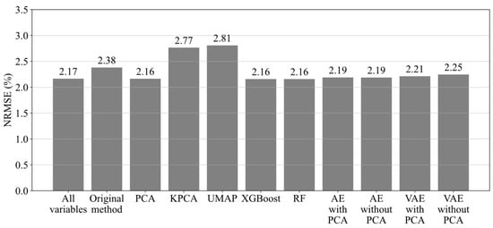
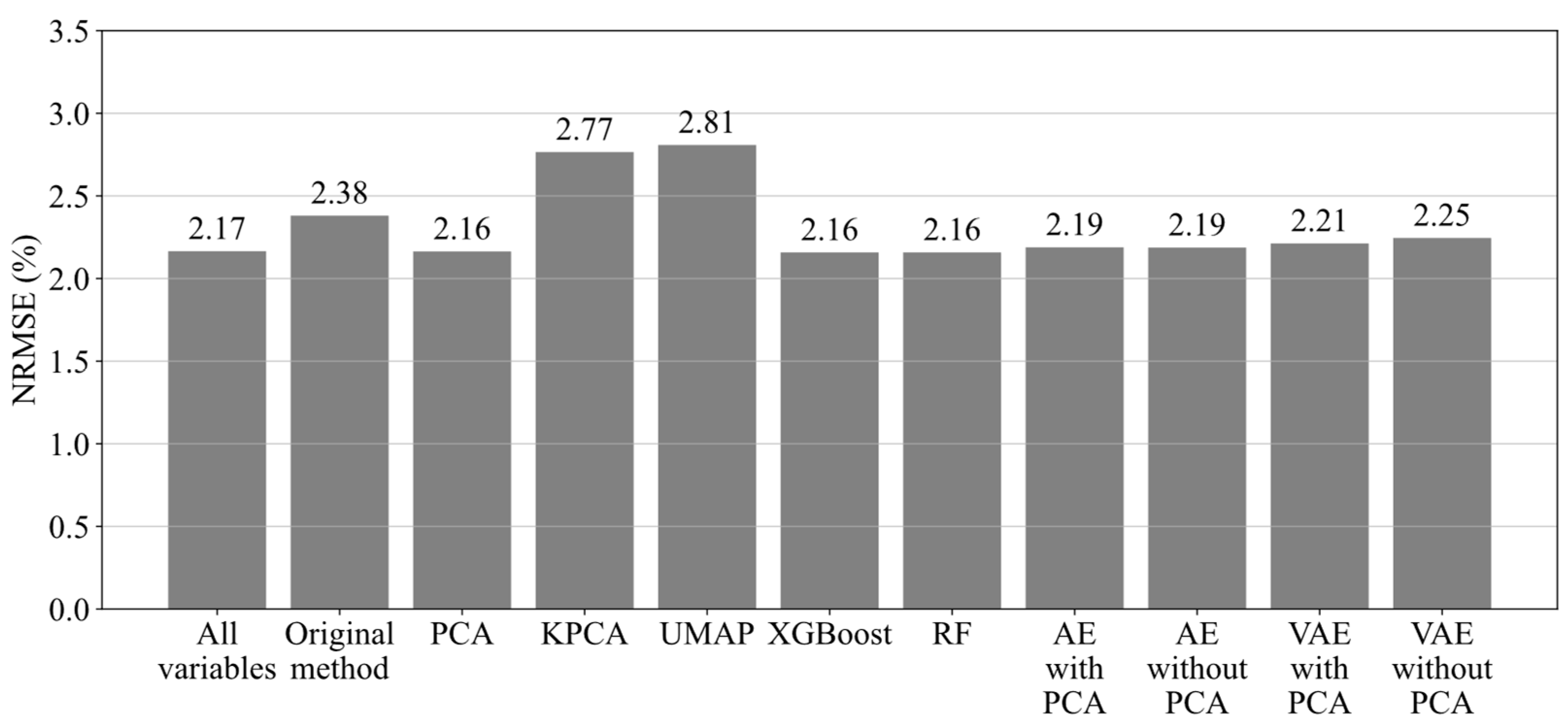
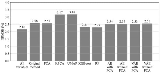
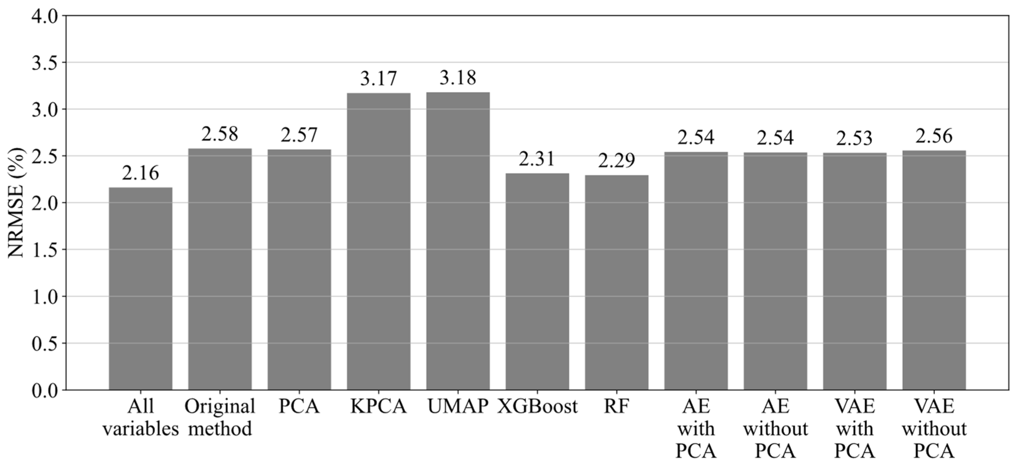
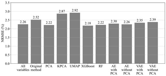
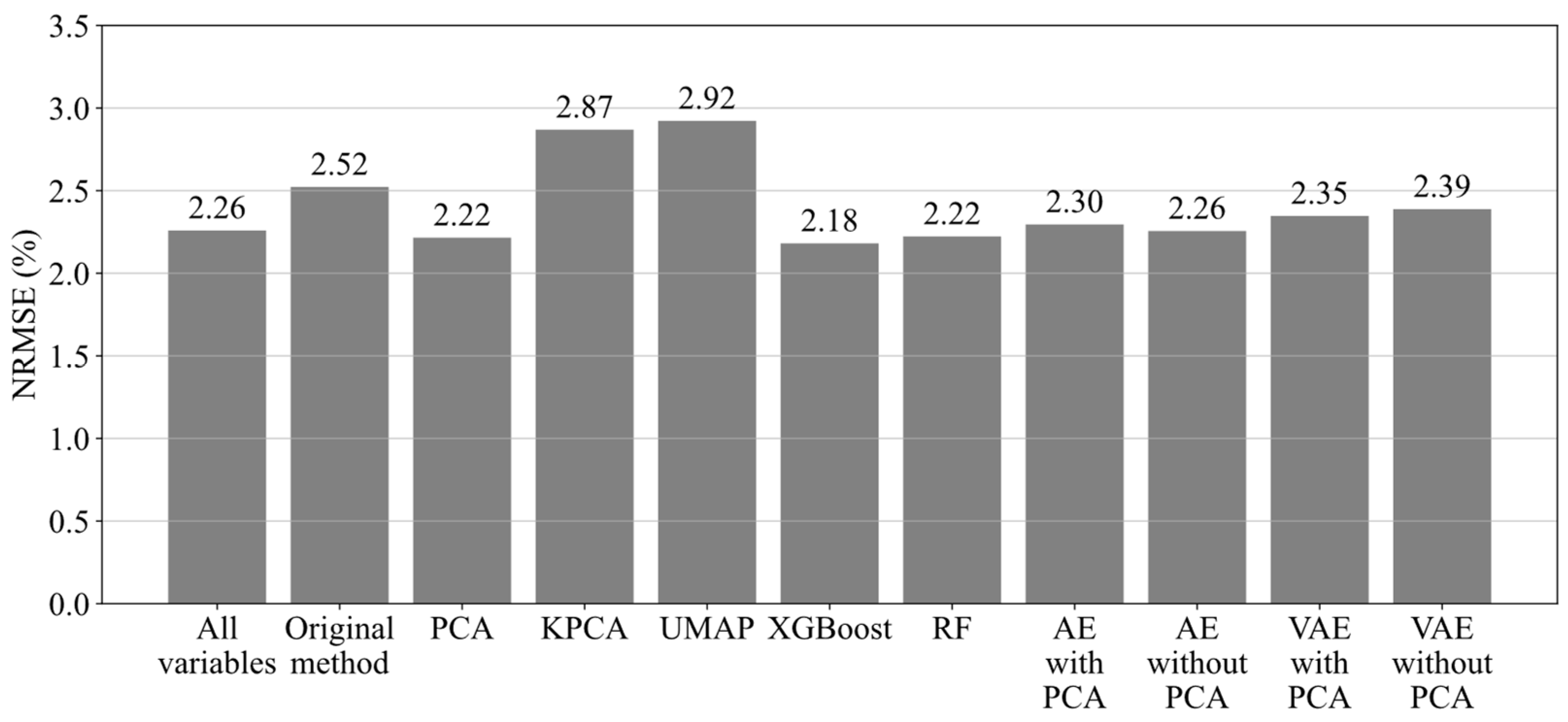

Disclaimer/Publisher’s Note: The statements, opinions and data contained in all publications are solely those of the individual author(s) and contributor(s) and not of MDPI and/or the editor(s). MDPI and/or the editor(s) disclaim responsibility for any injury to people or property resulting from any ideas, methods, instructions or products referred to in the content. |
© 2026 by the authors. Licensee MDPI, Basel, Switzerland. This article is an open access article distributed under the terms and conditions of the Creative Commons Attribution (CC BY) license.