


Abstract
Before CO2 is injected into an offshore saline aquifer, well injectivity is typically tested by injecting seawater. Because seawater differs chemically and thermally from formation water, the geochemical effect of this injection is uncertain. Here, the outcome of seawater injection into the Bunter Sandstone Formation, the main CO2-storage aquifer of the UK Southern North Sea, has been assessed using kinetic reactive transport models built in PHREEQC. These geochemical models use an equal-pore-volume radial grid and a time-staged wellbore temperature boundary. Twenty 30-day simulations comprised the reference case, single-factor variants and a factorial design of the injection rate, flow geometry and injected-water temperature, supported by grid, surface-area and activity-model tests. In every case, anhydrite cement dissolved behind a sharp front, raising near-well porosity from fractional 0.200 to about 0.226, with only minor dolomite precipitation. The front advanced in proportion to the volume injected and the anhydrite dissolution capacity of the seawater: the injection rate and flow geometry controlled its distance, while the temperature and activity model controlled the dissolution capacity. Translated to permeability, the porosity change implies an illustrative 10–25% increase in near-well aqueous injectivity, which requires confirmation via reactive core-flood experiments. The radial-grid and factorial workflow can be adapted to any aquifer, but the mineral reactions must be reassessed for each site.
1. Introduction
Anthropogenic emissions of carbon dioxide must be curtailed sharply and rapidly if global warming is to be limited to well below 2 °C above pre-industrial levels, and most credible pathways to that goal now rely on a combination of emissions reduction and active removal or the storage of CO2 [1]. Carbon capture and storage (CCS), in which CO2 captured from large point sources or from the atmosphere is injected into deep geological formations for long-term containment, is one of very few technologies capable of decarbonising sectors such as cement, steel and chemical production where emissions are difficult to eliminate via electrification alone, and it also underpins most scenarios for the negative emissions that will be needed if the Paris Agreement temperature targets are to be met [2]. Saline aquifers are attractive targets for CO2 storage because of their large potential capacity and their wide geographical distribution, but each prospective site must be assessed and tested before large volumes of CO2 can be injected with confidence.
A large proportion of the CCS projects proposed or under development worldwide and many of those in north-west Europe target offshore saline aquifers although depleted gas fields are also receiving a lot of attention as storage sites for CO2 [3]. Several considerations favour an offshore location for saline aquifers. Decades of hydrocarbon exploration and production have left many offshore sedimentary basins, including those beneath the North Sea, unusually well characterised in terms of their geology, so that formations suitable for CO2 storage can be identified and their capacity estimated with a level of confidence rarely available onshore [4,5,6]. The Bunter Sandstone Formation, for example, has been mapped and studied in detail across large swathes of the Southern North Sea Basin because of this hydrocarbon legacy [7]. Regulatory frameworks have typically already been established by oil and gas regulators [8,9]. Public acceptance of CCS tends to be greater when storage sites and any associated infrastructure are sited offshore and out of sight, and monitoring programmes designed for offshore storage can draw on well-established marine environmental monitoring practice [6]. Many saline aquifer CCS projects therefore have easy access to seawater.
Before a saline aquifer can be used to store CO2, its injectivity, meaning the rate at which fluid can be injected for a given pressure increase, must be demonstrated, and this is usually done via injection testing the well drilled into the target formation. Seawater is often used as the test fluid in offshore settings rather than CO2 itself. This is partly a matter of timing and logistics, because the pipelines, compressors and other topside equipment needed to deliver CO2 to an injection well in the required volumes are typically not ready when the well itself becomes available, whereas seawater can be drawn directly from the sea and injected with comparatively simple pumping equipment [10,11]. It is also a matter of cost, since large volumes of test-CO2 are expensive to produce, transport and inject, whereas seawater itself costs very little and the equipment needed to handle it is already familiar from decades of use in seawater injection for enhanced oil recovery [10,12]. Seawater injectivity tests therefore provide an early, low-cost indication of how a well and its surrounding formation will respond to fluid injection, ahead of the much larger commitment represented by CO2 injection. The Endurance structure in the Bunter Sandstone was itself appraised in this way: in 2013, the appraisal well 42/25d-3 was tested by injecting filtered seawater at 5000, 10,000 and 15,000 bbl/d at the top of the reservoir [13]. Saline water has been disposed of via injection into non-productive aquifer units in the Texas Gulf Coast for many decades; it was noted that injectivity tends to diminish with time [14]. This issue was explained as probably being the result of the migration of fine particulates from drilling mud, tank sludge or entrained solids in unfiltered injected brine, rather than scaling.
Injecting seawater into a saline aquifer is not, however, a purely physical process, because seawater is compositionally and thermally distinct from the resident formation water and will react with it and with the minerals present in the aquifer (Figure 1). The dissolution or precipitation of minerals such as anhydrite, dolomite and various aluminosilicate phases can enhance or reduce porosity and permeability in the near wellbore region and hence potentially have a direct bearing on the aquifer’s injectivity that a well test is intended to measure [15]. Geochemical reactive transport modelling, which couples fluid flow with thermodynamic and kinetic modelling of these mineral–water reactions, offers a means of anticipating such changes before a well test is carried out and of interpreting field observations of decreasing or increasing injectivity in terms of specific mineral reactions rather than as an unexplained departure from purely physical behaviour [12,16]. Modelling in advance of testing is particularly valuable where, as in many diagenetically complex sandstone reservoirs, several cement phases with different solubilities and reaction kinetics coexist and might reasonably be expected to respond differently to the injection of a cold, compositionally distinct fluid such as seawater [7].
Figure 1.
Seawater injectivity testing as a proxy for CO2 injection. Seawater (about 10 °C) is warmed as it descends the well, by an amount that decreases with time as the surrounding rock cools. In the aquifer (56 °C), it displaces and mixes with formation water, reacts with the host minerals and cools the rock near the well. The study asks whether these reactions cause mineral scale (damage), mineral dissolution (enhancement) or petrophysically neutral change.
Undertaking a geochemical reactive transport model of this kind requires several categories of data. The mineralogy of the reservoir rock, established through X-ray diffraction, petrography and scanning electron microscopy, is needed to define which mineral phases are present and in what proportions, since this determines which reactions are possible [7]. The chemical compositions of both the resident formation water and the injected fluid are required as the starting point for any reaction calculation, together with the temperature, pressure and, where the injected fluid is expected to warm progressively as it moves away from a cold wellbore, the thermal history of the fluid during injection. Finally, a thermodynamic and kinetic database is needed that provides equilibrium constants and rate laws for the relevant mineral–water reactions at reservoir temperature and pressure; the calculations reported here were performed using PHREEQC [17] together with the Kinec_v3 database [18].
In this study, PHREEQC reactive transport modelling has been used to examine the geochemical consequences of injecting cold seawater into the Bunter Sandstone Formation, a saline aquifer at approximately 56 °C in the Southern North Sea, as a proxy for the injectivity testing that would precede CO2 injection at such a site. Twenty model variants were run: a reference case and six single-factor variants of it, seven further models completing a factorial design and six supplementary variants testing halite in the initial mineralogy, formation-water sulphate, reactive surface area and grid size. These twenty models were run in order to establish which aspects of the geochemistry are robust and which are sensitive to how the problem is represented. The results here are presented as a series of figures intended to convey both the overall behaviour of the system and, where relevant, the specific mineral reactions responsible for it. The study addresses two questions:
- When cold seawater is injected into a saline aquifer as a proxy for CO2-injectivity testing, do geochemical reactions with the reservoir minerals and the native formation water damage injectivity (mineral scale/precipitation) improve injectivity (dissolution and porosity increase) or leave it essentially unchanged?
- Given that a full reactive transport model requires numerous simplifying choices, which of those choices are most important for the predicted outcome?
2. Data and Methods
2.1. Wellbore Heat Transfer: The Ramey Method
Seawater is injected at the wellhead significantly below the reservoir temperature, and it exchanges heat with the surrounding rock as it descends the wellbore, so the fluid that reaches the perforations is at neither the injection temperature nor the undisturbed reservoir temperature. Mineral equilibria, kinetic reaction rates and gas solubility all depend on the temperature, so the bottom-hole fluid temperature is a required input to the reactive transport model.
Heat transfer across the tubing, annulus, casing and cement reaches a steady state within minutes of the start of injection and can be treated as instantaneous, but the conduction of that heat into the surrounding formation cannot. The rock disturbed by cooling grows outward as the square root of the elapsed time, so thermal resistance between the wellbore and the undisturbed formation rises through the injection period. Ramey [19] combined a steady-state wellbore with a transient formation into a single depth-dependent equation for the fluid temperature. For fluid injected at temperature Tinj into a formation with undisturbed temperature Te(z) = Tsb + Gz, where G is the geothermal gradient, the fluid temperature at depth z and time t is as follows:
where A(t) is a relaxation distance, the depth over which the fluid and formation temperatures converge and lengthens as the disturbed rock annulus widens with time. A longer A(t) lets more of the wellhead-to-formation temperature difference survive to depth z, so bottom-hole temperature drifts towards the injection temperature as injection continues.
Tf(z,t) = Te(z) − A(t)G + [Tinj + A(t)G − Tsb] exp[−z/A(t)]
Ramey [19] derived the time function within A(t) from the line-source solution for transient radial conduction, the same mathematics that underlies the Theis well function in groundwater hydrology. A closed-form large-time approximation of the type given by Hasan and Kabir [20] was used here to generate the time-staged boundary temperature applied at the injection cell. Hagoort [21] tested Ramey’s approximation against a rigorous transient solution and found it accurate for most of the injection period, departing from the exact solution only in an early transient window, hours to a few days depending on well and formation properties, during which the method overstates the fluid-to-formation temperature difference. Willhite [22] separately resolved the overall heat-transfer coefficient into its tubing, annulus, casing and cement components and validated the approach against measured casing temperatures during steam injection, of which a single effective conductivity, as used here, is the simpler limiting case. The method remains current in the geological setting relevant to this study: it was applied to wells in the Prinos–Kavala Basin to estimate the wellhead temperature ahead of CO2 injection [23].
The Ramey [19] temperature schedule, computed for the seawater injection rate, wellbore geometry and injection duration used in this model, was applied as nine discrete boundary-temperature stages spanning day 1 to day 30 of the simulated injection period. Cooling of the injected fluid is most rapid soon after breakthrough at the perforations and progressively slower thereafter, and this staged schedule represents that behaviour within the reactive transport model in a stepwise but reasonably continuous fashion. At 10,000 bbl/d, the resulting bottom-hole temperatures at days 1, 2, 3, 5, 7, 10, 14, 21 and 30 were 14.5, 13.7, 13.3, 13.0, 12.8, 12.6, 12.4, 12.3 and 12.2 °C, and at 1000 bbl/d they were 36.5, 33.7, 32.2, 30.6, 29.7, 28.8, 28.0, 27.1, and 26.4 °C; every input to the calculation is listed in Table 1. Whatever values these inputs take, the bottom-hole temperature must lie between the seawater intake temperature (10 °C) and the reservoir temperature (56 °C), so models M3 and M4 bracket the range of bottom-hole temperatures considered in the present high-rate sensitivity analysis (Section 3.3).
Table 1.
Inputs used for the Ramey calculation of injected seawater temperature.
All reservoir cells were initially at 56 °C. Heat transport was calculated using PHREEQC’s TRANSPORT formulation, with a dimensionless temperature-retardation factor of 2.96 to represent heat storage in the rock–water system and a thermal diffusion coefficient of 1.0 × 10⁻⁶m2 s−1. The heat and solute transport were assigned the same dispersivity in each grid cell. At 10,000 bbl/d, the inlet temperature was held at 14.51, 13.69, 13.34, 12.97, 12.78, 12.59, 12.44, 12.28 and 12.16 °C over successive intervals ending at approximately days 1, 2, 3, 5, 7, 10, 14, 21 and 30, respectively; the first interval began at injection onset. The corresponding inlet temperatures at 1000 bbl/d were 36.51, 33.65, 32.22, 30.63, 29.70, 28.79, 28.01, 27.14 and 26.44 °C for the nine successive stages, respectively.
2.2. Pseudo-Three-Dimensional Radial Grid Construction
PHREEQC’s TRANSPORT keyword solves the one-dimensional advection-dispersion-reaction equation along a single string of cells [17], and nothing in that formulation restricts the cells to a Cartesian, one-directional flow path. In this model, each cell instead represents a concentric annular shell around the injection well, of net thickness h, so that a formally one-dimensional sequence of cells reproduces a three-dimensional, radially symmetric flow geometry. The construction is pseudo-three-dimensional in this sense: each cell carries a real cylindrical-shell volume rather than a notional unit cross-section, while the transport calculation itself still advances along a single spatial coordinate, radius r, with no separate angular or vertical flux terms.
A radial grid was chosen because flow around a vertical injection well is radially divergent rather than one-directional. A Cartesian grid block reproduces the correct near-well pressure and concentration field only through a specific equivalent wellbore radius rather than at the block centre [24], and a radial grid removes the need for this correction.
Each cell occupies the annulus between radii ri − 1 and ri and has bulk volume:
Vi = πh(ri2 − ri−12)
An equal-width radial grid would produce annular cells whose volumes increase approximately linearly with the radius, giving progressively longer residence times at a fixed volumetric flow rate. To maintain equal cell volumes and residence times, the grid used here instead holds the increment in the squared radius constant across all cells: , where C=Δr1(Δr1 + 2r0) is determined by the wellbore radius, r0, and the chosen first-cell width, Δr1. Every subsequent boundary radius is given by the following:
ri = √(r02 + iC)
This produces cells of monotonically decreasing width outward (Figure 2), the reverse of an equal-width grid, while giving every cell the same bulk and, because porosity is uniform, the same pore volume.
Constant pore volume per cell has a direct numerical benefit at a fixed injection rate, Q: a single scalar time step, Δt = φπhC/Q, where φ is porosity, applies uniformly along the whole grid [17]. An equal-width grid would instead need either a variable time step or a Courant number varying by orders of magnitude across the domain, because the cell pore volume would then increase with the radius while the flux through each cell’s outer annulus is conserved.
Dispersivity was set to one-tenth of the width of each cell of a 45-cell grid (αi = 0.1Δri), consistent with the widely used approximation that longitudinal dispersivity is about one-tenth of the scale of observation [25], giving a uniform grid Péclet number of 10 on that grid. In the 90-cell reference grid, each cell of the 45-cell grid is split into two cells of equal pore volume, and both keep the dispersivity of the cell that they subdivide. Because both column ends used flux boundary conditions, PHREEQC’s -correct_disp option was applied, which scales dispersivity by (1 + 1/n) for the n-cell column [17]. Dispersivity therefore decreases outwards in the radial grid but is unchanged by grid refinement, so the grid-refinement test (Section 3.5) changes the numerical resolution only, not physical dispersion.
Because the cross-sectional area available to the flow, 2πrh, grows with the radius, interstitial velocity in the radial grid falls off as 1/r for a fixed volumetric injection rate, in contrast to the constant velocity of a linear, core-flood-style column of a fixed cross-section [24]. This distinction has direct consequences for reactive transport: comparisons of radial and linear flow under otherwise similar conditions show different dissolution and front-propagation behaviour because the flow field itself differs between the two geometries [26], which is the basis for the radial-versus-linear sensitivity test reported below.
PHREEQC has previously been run on a radial or axisymmetric grid outside the CO2-storage literature: to model radial tracer diffusion through Opalinus Clay [27], an application now built into PHREEQC version 3 as a worked example [17], to interpret single-well push–pull tests in an aquifer storage and recovery setting [28] and, coupled to an external flow code, to predict reactivity around a geothermal CO2-dissolved injection doublet [29]. However, it seems that the PHREEQC radial grid approach has not previously been applied to CO2 storage or waterflood injectivity, so the equal-pore-volume construction used here extends a documented but discipline-scattered technique into this application.
Figure 2.
Schematic representation of the pseudo-3D grid elements employed in most of the PHREEQC geochemical reaction-transport models.
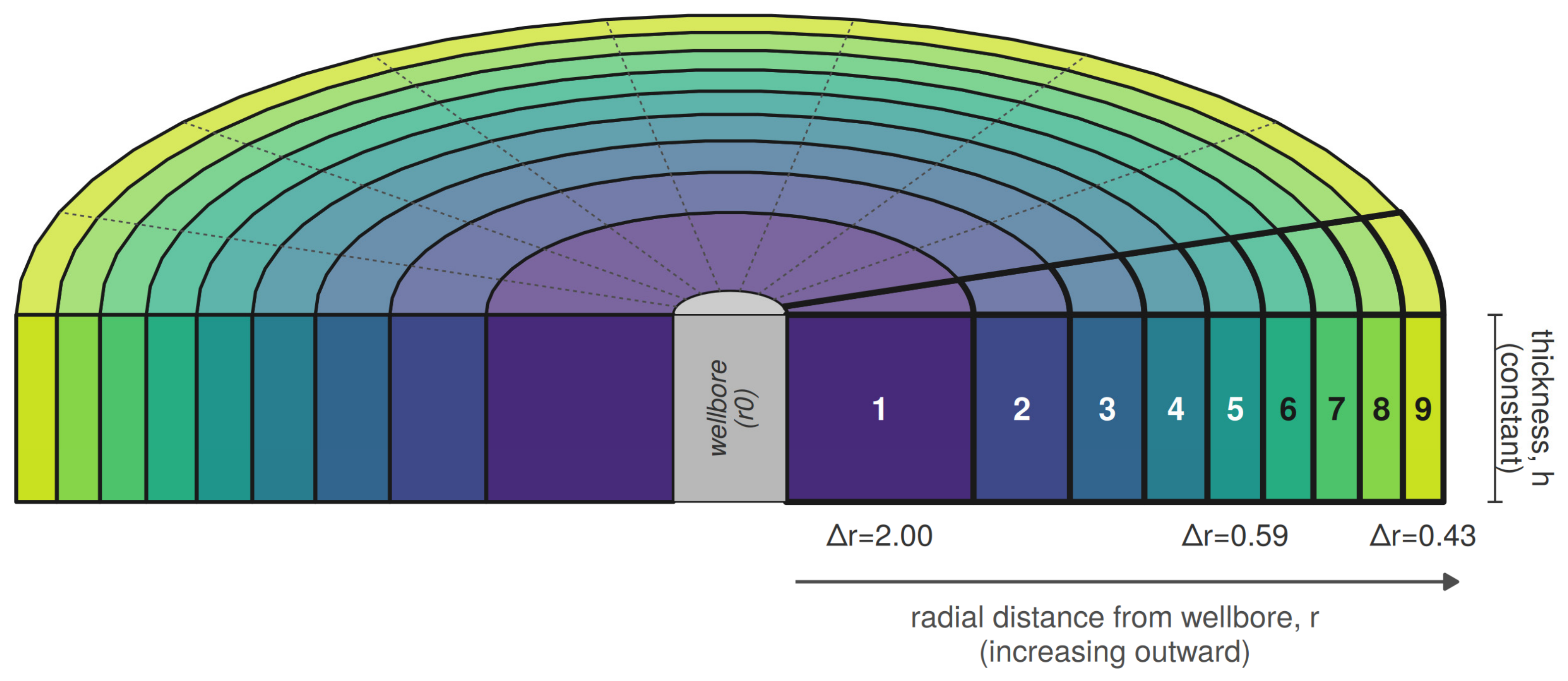
This representation carries several assumptions. The reservoir is taken to have a uniform net thickness, h, and uniform porosity, φ, over the modelled radius. Properties are assumed to be homogeneous in the angular direction, so that the three-dimensional cylindrical problem reduces to a function of the radius alone. Permeability is assumed to be isotropic in the horizontal plane, keeping flow lines radial rather than distorted towards a preferred direction. Flow is assumed to be single-phase, with the pore space remaining fully water-saturated throughout, so that the pore volume displaced equals the volume injected. The injection rate, Q, is held constant, which is what allows the single scalar time step derived above to apply for the whole simulated period. The grid resolution and domain extent are also coupled rather than independent, because C is fixed once r0, Δr1 and the cell count, N, are chosen, so narrowing the near-well cell without adding cells reduces the modelled outer boundary radius. In the models reported here, the wellbore radius, r0, is 0.108 m, the outer boundary lies at 9.53 m and the assumed net thickness, h, is 50 m. The reference grid has 90 cells (45 in the grid-refinement comparison), giving a first-cell width of about 0.90 m, and at 10,000 bbl/d (1590 m3/d), the time step is about 1722 s.
The grid, kinetic mineral assemblage and radial transport scheme were implemented in PHREEQC version 3 [17] using the TRANSPORT keyword with cell-specific -lengths and -dispersivities arrays, -correct_disp enabled and a single -time_step and -shifts pair. Output from PHREEQC was processed in Excel and plotted using ggplot2 in R version 4.5.1 (2025-06-13 ucrt) [30].
2.3. Geochemical Reactive Transport Modelling: PHREEQC, Kinec_v3 and Pitzer
All reactive transport calculations were carried out in PHREEQC version 3 [17], a public-domain geochemical code that solves aqueous speciation, mineral equilibrium, kinetic reaction and one-dimensional transport problems within a single ion-association thermodynamic framework. Aqueous species activities are calculated from the composition specified in each SOLUTION block, mineral saturation states follow from comparing the resulting ion activity products with equilibrium constants held in the thermodynamic database and reaction proceeds, either instantaneously to equilibrium (EQUILIBRIUM_PHASES) or at a rate set by a user-defined rate law (KINETICS and RATES), until the solution and mineral assemblage are mutually consistent at each time step.
Kinec_v3 was the database used for 19 of the 20 models [18]. Kinec_v3 uses a slightly modified version of the CarbFix thermodynamic database [31] and the EQ3/6 B-dot activity model [32].
Mineral dissolution and precipitation rates followed the Kinec_v3 database [18], which supplies Arrhenius-type rate laws, dependent on an activation energy term, for the major silicate, aluminosilicate, sulphate and carbonate minerals present in the Bunter Sandstone assemblage, so that reaction rate responds automatically to the cell temperature computed from the Ramey [19] schedule described above.
Kinec_v3′s native activity-coefficient formulation, an extended Debye–Hückel type expression [32], is strictly applicable only at ionic strengths below roughly 1 mol/kgw, whereas the displaced Bunter Sandstone formation water modelled here has an ionic strength of around 4 mol/kgw. This brine is, however, displaced from the near-well domain within about two days of injection, after which the anhydrite front advances into seawater-dominated water with an ionic strength of about 0.6–1.0 mol/kgw, which is within the accepted range for the extended Debye–Hückel-type expression for activity coefficients [32]. To test the sensitivity of the modelled injectivity outcome to this limitation, one model used a database merging the Kinec_v3 kinetic rate laws with the Pitzer ion-interaction activity model. Because PHREEQC’s Pitzer dataset [33] lacks Al and Fe species and quartz, aluminosilicate and Fe phases proved unreactive over 30 days (M1 vs M2, below), these phases were omitted from a merged database that combines Pitzer [34] ion-interaction parameters for Na, K, Ca, Mg, HCO3, SO4 and Cl with the Kinec_v3 rate laws. M7 was therefore treated as a database-formulation sensitivity test, retaining the Kinec_v3 kinetic rate laws but using Pitzer aqueous thermodynamics.
Each model required four categories of input. The chemical composition of the resident Bunter Sandstone formation water and of the injected North Sea seawater was specified as PHREEQC SOLUTION blocks. The initial mineral assemblage of the reservoir rock, expressed as volume fractions, was specified as EQUILIBRIUM_PHASES or KINETICS blocks with starting moles calculated from measured or estimated modal mineralogy. Kinetic rate parameters for each mineral were taken from Kinec_v3 or from the merged Pitzer-Kinec_v3 database for the model described above and implemented through RATES blocks. Finally, the transport geometry and boundary conditions comprised the radial or linear grid, the dispersivity array, the injection rate, the simulated duration and, where applicable, the Ramey-derived boundary temperature schedule.
For every cell and every reported time step, PHREEQC’s USER_PUNCH facility was used to output pH, the concentrations of the major solutes (Ca, Mg, Na, K, Cl, SO4, HCO3 and others), the saturation index of each mineral in the assemblage and the number of moles and the volume of each mineral phase present, from which the fractional mineral abundance and bulk porosity change were calculated directly. These outputs, generated for each of the 90 cells at each of the discrete simulated times reported in the figures, form the basis for the comparison of the twenty models presented below.
2.4. Data Used in the Model
The modal (XRD) mineralogy (Table 2) and formation water composition (Table 3) used to build the PHREEQC model are those reported for the Endurance saline aquifer, within the Bunter Sandstone Formation, during the front-end engineering design of the White Rose CCS Project [35], supplemented by the more recent, peer-reviewed core-based petrographic characterisation of the same formation at the 43/28-NEPBH1 borehole, some 30 km along the Bunter Sandstone hydraulic unit from Endurance [36]. The two sources agree on the broad diagenetic mineral suite present: an arkosic sandstone framework of quartz, K-feldspar and albite, overprinted by dolomite, anhydrite, hematite and authigenic illite. Halite reported in petrographic core samples is assumed to be an artefact of the evaporation of saline formation water once the core has been allowed to dry out because the formation water is saline but still strongly undersaturated with halite (see next paragraph). Halite cannot exist under equilibrium conditions as a discrete mineral in these sandstones in contact with the reported formation water. Note that halite dissolution kinetics are so fast [18] that halite would rapidly dissolve until halite saturation is reached and the formation water salinity would be raised far in excess of that of the reported formation water (Table 3). The mineral assemblage, the renormalised XRD-derived volume fractions and the resulting mass and molar quantities used as PHREEQC KINETICS input are given in Table 2.
The nominal formation water composition used in this study and the composition adopted for the injected seawater are presented in Table 3; Triassic Bunter formation water compositional data have been collated from various sources [35,37]. The formation water is saline and is dominated by Na and Cl and is about 50% saturated with halite (i.e., the ion activity product is about half the halite solubility product). The water also has an elevated concentration of Ca. The reported formation water [35] composition is about 10 to 25% saturated with anhydrite (depending on which activity model is employed); this is incompatible with the routinely reported presence of anhydrite in the Bunter Sandstone Formation [7,36,38]. The attainment of equilibrium of Bunter formation water with anhydrite, ahead of any seawater injection, has been assumed, thus raising the aqueous sulphate concentration to about ten times the reported values. It is here speculated that the water analyses reported were undertaken on samples following cooling, depressurisation and CaSO4 mineral formation. If this important modification of the reported water chemistry had not been undertaken, then the PHREEQC simulation would have led to the kinetically controlled dissolution of anhydrite in the rock even without any injection of seawater.
Rather than a North Sea-specific seawater analysis, the injected fluid was assumed to be Standard Seawater, the reference open-ocean composition [39,40]. An operational assessment should use an analysis of the seawater to be injected.
The reactive surface area (Table 2) is the least constrained model input, typical of most geochemical modelling studies [41,42]. Laboratory BET measurements are made on disaggregated powders and tend to inflate the surface area relative to intact grains [43,44], while SEM and micro-CT imaging have resolution and representativity limits, and published values for a single mineral can span several orders of magnitude: for example, the reported illite specific surface area ranges from about 0.015 to 46 m2/g. A common way to reconcile these extremes is to scale a geometric or BET surface area by a roughness or accessibility factor, f-r, that reduces the theoretical mineral surface to the fraction actually available to the reaction [45]. Following this approach, a geometric specific surface area was calculated for each kinetic mineral from an assumed grain size and shape, around 250 micrometres for the sand-grade framework and about 25 micrometres for the sulphate and carbonate cement minerals of the Bunter Sandstone, together with the mineral’s crystal density, and this geometric value was then scaled by a mineral-specific f-r of between 0.1 and 0.5. The resulting specific surface areas, between 0.03 and 0.05 m2/g for the carbonate and sulphate phases in this model (Table 2), sit between the lower values used by Gaus et al. [46] for reactive transport modelling of the Sleipner caprock and the higher values reported by Xu et al. [45] and are applied within PHREEQC’s mass-normalised surface-area formalism [47] as retained in Kinec_v3 [18].
Five model-conditioning assumptions underlie the results and are tested where possible: (i) the formation water was pre-equilibrated with anhydrite, raising sulphate from 385 to 3903 mg/kgw (tested in Section 3.10); (ii) halite was excluded from the mineral assemblage because the formation water is undersaturated with respect to it (tested in Section 3.10); (iii) the injected fluid is Standard Seawater; (iv) the aluminosilicate, oxide and sulphide minerals are inert over 30 days (tested by M1 against M2, see Section 3.2); and (v) net thickness, porosity and injection rate are uniform and constant (Section 2.2). Gypsum was not included as a secondary phase. Near-well temperatures in the cold-injection models (about 12–37 °C) lie mostly below the gypsum–anhydrite transition temperature, about 42–58 °C in pure water depending on the study and lower in saline water [48], but unseeded anhydrite in contact with water at such temperatures persists metastably for months without converting to gypsum [49,50], so replacement of anhydrite by gypsum is not expected within a 30-day test (see Section 4.3).
Table 2.
Modal mineralogy of the Bunter Sandstone Formation reservoir.
Table 3.
Chemical composition in mg/kgw of the injected seawater and Bunter formation water 1.
2.5. Mineral Mass-Balance Conversions: From Modal Mineralogy to Kinetic Input, and from Reaction Progress to Porosity
PHREEQC’s KINETICS block requires the starting amount of each reactive mineral, m0, in moles per kilogram of pore water, rather than as the volume percent reported by point counting or XRD. Converting between the two requires the initial porosity described above [51], because it fixes how a unit volume of reservoir rock splits between the mineral matrix and pore space and hence how much pore water is available to normalise the mineral inventory against. The conversion itself was made in three steps. First, the volume fraction of a given mineral, referenced to the solid matrix fraction of a unit rock volume fixed by the initial porosity, was converted to a mass by multiplying by its crystal density: mass = volume fraction × matrix volume × density. Second, that mass was converted to an amount in moles by dividing by the mineral’s gram formula weight, taken from the thermodynamic database [17]. Third, because PHREEQC expresses all solute and mineral amounts relative to the mass of water (1 kg of water is the standard reference for PHREEQC) in solution rather than to the rock volume, the resulting amount was divided by the mass of pore water contained in the same unit rock volume, itself equal to porosity × unit volume × water density, to give the value in moles per kilogram of water entered into the KINETICS block [17]. The density and gram formula weight together define a mineral’s molar volume, so this conversion is equivalent to dividing the mineral volume directly by its molar volume, and tabulated molar volumes from the thermodynamic database were used for this purpose in the model build.
The same three-step conversion was applied in reverse to interpret the model output and derive porosity, again anchored to the same initial porosity value [51]. At each reported cell and time, PHREEQC’s USER_PUNCH facility returns the amount of every mineral present, in moles per kilogram of water, including minerals held chemically inert over the 30-day simulation, as well as those reacting kinetically. Each amount was converted back to a volume by multiplying by the mineral’s molar volume, and the volumes were summed across the whole assemblage, inert and reactive alike, because an inert mineral still occupies the pore-filling volume even though its amount does not change. The resulting total mineral volume was compared with its initial value, itself calculated from the same modal mineralogy and initial porosity used to set up the model, to give a volume change. This change was expressed as a fraction of the constant total, mineral plus pore, volume associated with the same kilogram of water, a total fixed by the initial porosity on the assumption that the bulk rock volume itself does not change during the simulated injection period. Adding this change to the initial porosity gives the porosity at each cell and time, reported throughout as a fraction of bulk rock volume.
3. Results
Twenty variants of the PHREEQC reactive transport model were run (Table 4), all defined against a common reference case (M2) and using the mineral assemblage, formation water and seawater compositions given in Table 2 and Table 3. Models 1 to 7 will be presented in detail (Figure 3, Figure 4, Figure 5, Figure 6, Figure 7, Figure 8, Figure 9, Figure 10, Figure 11, Figure 12 and Figure 13), and then, 12 of the 14 models will be compared in factorial analysis figures (Figure 14, Figure 15 and Figure 16). Model 1 (M1) is the full-kinetics model, in which all sixteen minerals present (Table 2) in the assemblage, including quartz, the feldspars, hematite and illite, react kinetically using the Kinec_v3 database, a radial grid, staged Ramey cooling and an injection rate of 10,000 bbl/d. Model 2 (M2) is the reference case used for every subsequent sensitivity test: it freezes the eight minerals shown in the following section to be unreactive on the 30-day timescale of interest, leaving only the eight carbonate and sulphate phases kinetically active and otherwise uses the same radial grid, staged Ramey cooling and injection rate as M1. Models 3 to 7 each isolate one further choice against M2: an isothermal injection temperature (M3), a fixed cold injection temperature held for the full 30 days (M4), linear rather than radial flow (M5), a tenfold lower injection rate (M6) and the Pitzer activity model in place of Kinec_v3′s native extended Debye–Hückel formulation (M7). Six supplementary runs test the grid resolution (M2 and M5 on a 45-cell grid), reactive surface area (M2 with anhydrite and dolomite surface areas doubled and halved) and two input assumptions (M2 with a halite volume fraction of 0.05 and M2 with the reported formation-water sulphate); they are reported in Section 3.5, Section 3.9 and Section 3.10.
3.1. The Initial Case: All Minerals Treated as Kinetic Inputs, Injection Design and the Porosity Response (Model 1)
The temperature of the injected seawater at the top of the reservoir depends strongly on injection rate (Figure 3A). The water gains little heat in the wellbore and arrives at about 12 °C after the first few days and stays close to that value for the remainder of the 30-day period at 10,000 bbl/d. Conversely, the longer residence time allows more heating, and the water stays above 26 °C at 1000 bbl/d.
Porosity rises from its initial value of 0.20 (Table 2) to around 0.226 in the zone swept by seawater and stays at the background value ahead of an advancing reaction front (Figure 3B). The front is sharp at every step examined, moving from around 1.1 m from the well after one day to around 5.7 m after 30 days, with its rate of advance slowing progressively through the simulation. Throughout this paper, the front position is the distance from the well of the first cell in which the fractional anhydrite volume exceeds half its far-field value. Plotted instead as a function of time at fixed distances from the well (Figure 3C), the same behaviour appears as an abrupt breakthrough at each cell, arriving sooner the closer the cell lies to the injection point; the cell at 9 m is not reached at all within the simulated 30 days. This zone of increased porosity would be expected to improve near-well injectivity.
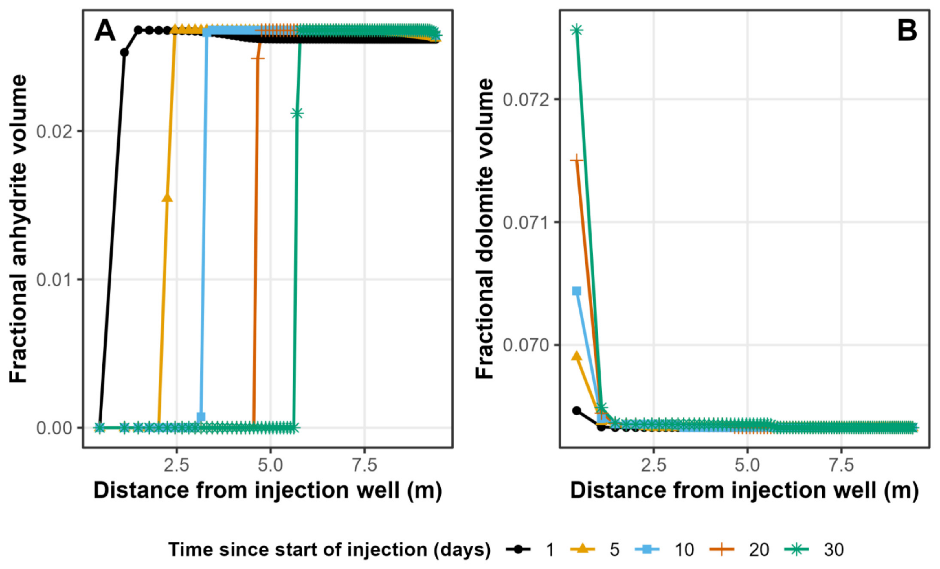
Anhydrite dissolution is the process responsible. The fractional anhydrite volume falls from around 0.026 to 0.000 behind the front and remains close to its background value ahead of it, and the position of the anhydrite dissolution front coincides with the porosity front at every time step (Figure 4A). Dolomite shows a much smaller, opposite response: a modest increase in fractional volume in the cells in longest contact with the injected water, highest immediately adjacent to the wellbore and decaying to background within about 1.5 m (Figure 4B). The vertical scale in Figure 4B is roughly forty times finer than in Figure 4A; therefore, anhydrite dissolution dominates the volume change.
Figure 3.
Injection design and porosity response (Model 1). (A) Imposed boundary temperature of the injected seawater over the 30-day injection period, for both injection rates modelled. (B) Fractional porosity versus distance from the well at five times during injection. (C) Fractional porosity versus time at four fixed distances from the well.
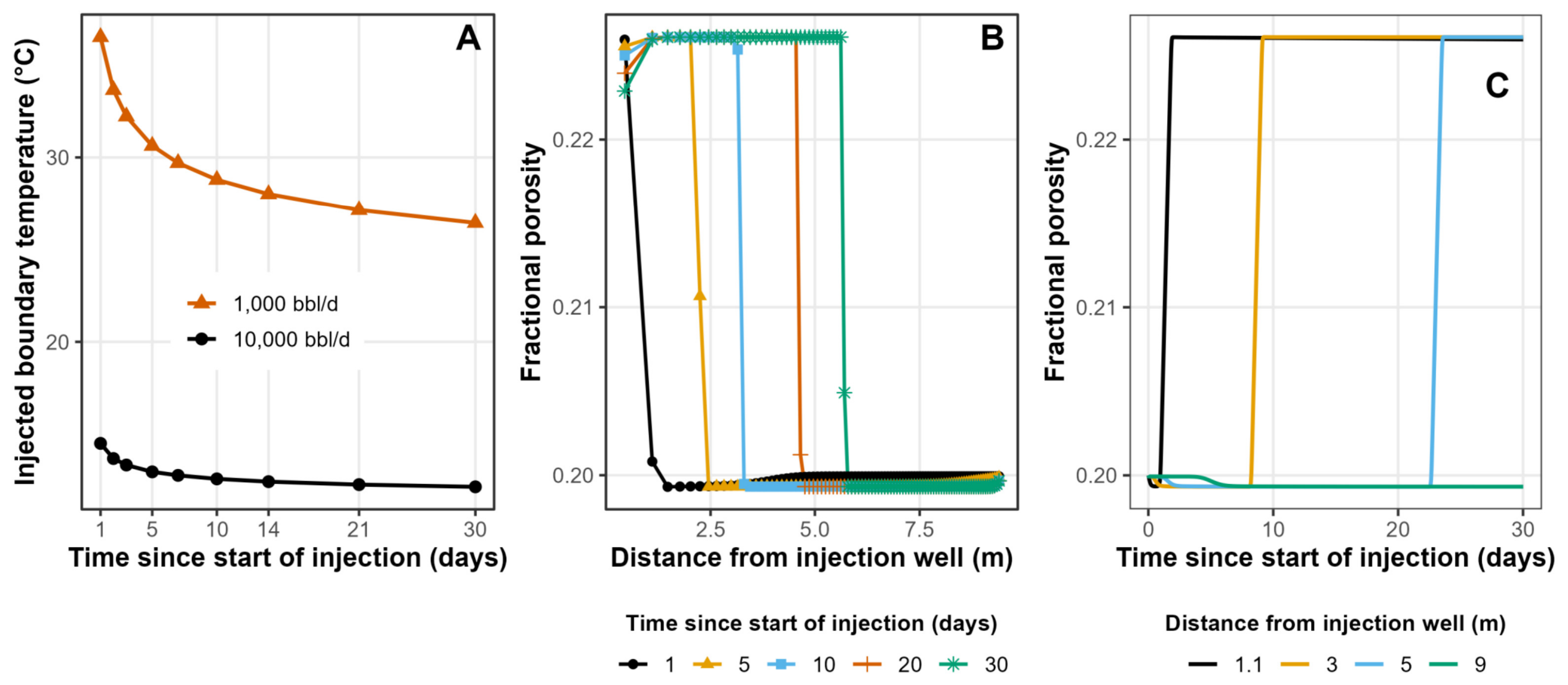
Figure 4.
The two minerals that control the porosity change (Model 1). (A) Fractional anhydrite volume versus distance, at the same five times as Figure 3. (B) Fractional dolomite volume versus distance, at the same times; note the finer vertical scale.
The solution chemistry accompanying this mineral response is shown in Figure 5. On day 1, pH is about 6.9–7.0 next to the well and falls to a minimum of about 6.45 at about 7 m, where the injected seawater meets the displaced formation water; by day 30, pH is about 7.2 behind the anhydrite front and about 6.9 ahead of it (Figure 5A). The pH is controlled by the carbonate and sulphate minerals, which react kinetically throughout the grid. The day-1 minimum coincides with the seawater–formation-water mixing zone shown by Mg (Figure 5D), not with the anhydrite front, which lies at about 1.1 m on day 1 (Figure 5B).
Figure 5.
Solution chemistry accompanying the reaction (Model 1). (A) pH versus distance. (B) Anhydrite saturation index versus distance. (C–E) Dissolved Ca, Mg and SO4 versus distance, day 1 compared with day 30.
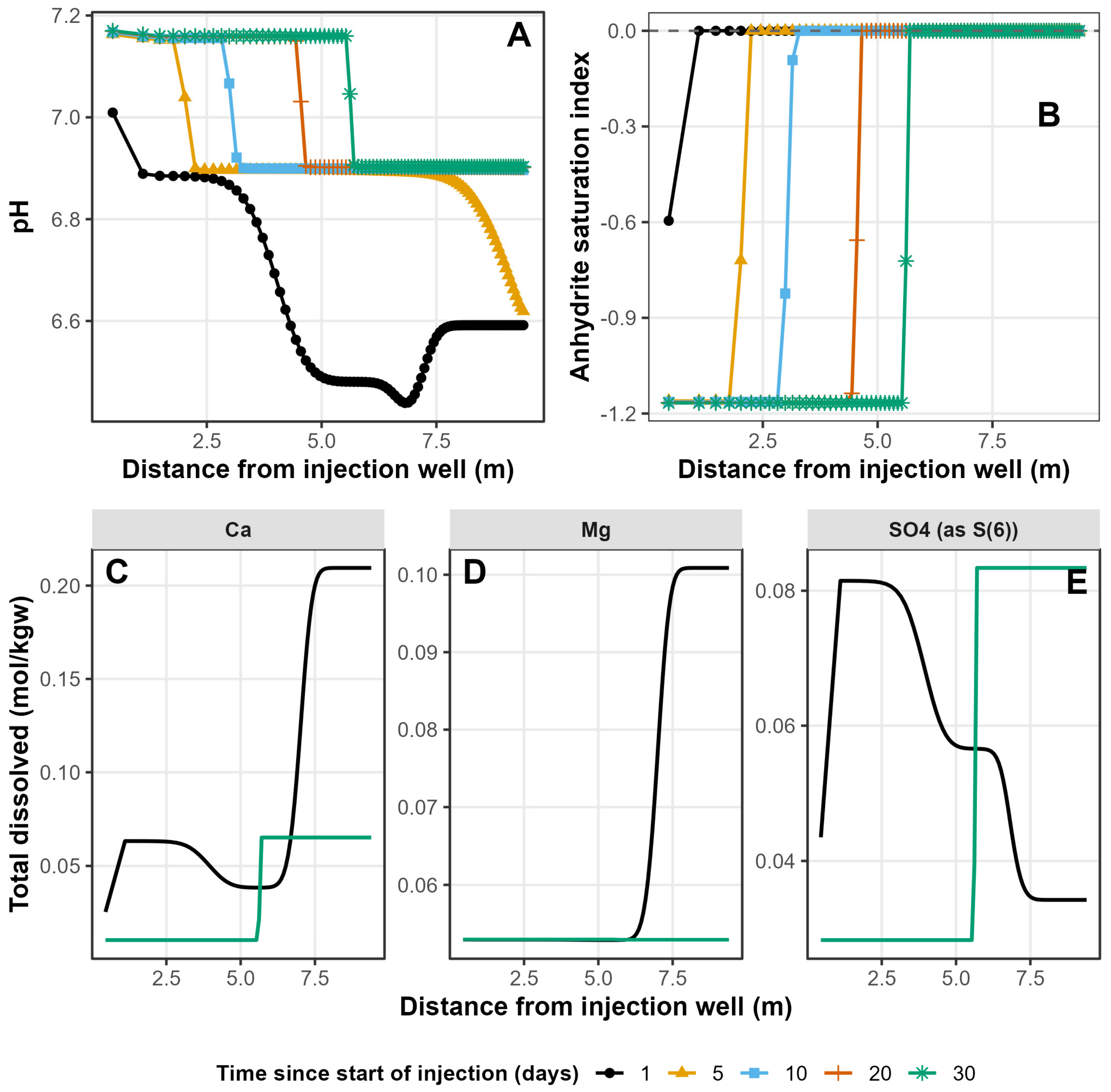
The anhydrite saturation index is about −1.17 in the injected seawater ahead of the point of re-equilibration and returns to zero, the equilibrium value, at the same distance where the anhydrite dissolution front sits (Figure 5B). Dissolved Ca and SO4 track this same front closely, both showing a sharp, retarded step at the same position and advancing only slowly between day 1 and day 30 (Figure 5C,E). Dissolved Mg behaves differently: its mixing zone already extends to 6 to 8 m by day 1, well ahead of the day-1 reactive front at around 1.1 m, and by day 30, the entire modelled domain has been swept to the low, seawater-like Mg value (Figure 5D). Because dolomite growth is volumetrically minor, Mg is only weakly retarded by the reaction and is transported largely as a conservative species, running well ahead of the anhydrite-buffered porosity front rather than tracking it.
3.2. Can the Aluminosilicate, Oxide and Sulphide Minerals Be Treated as Inert?
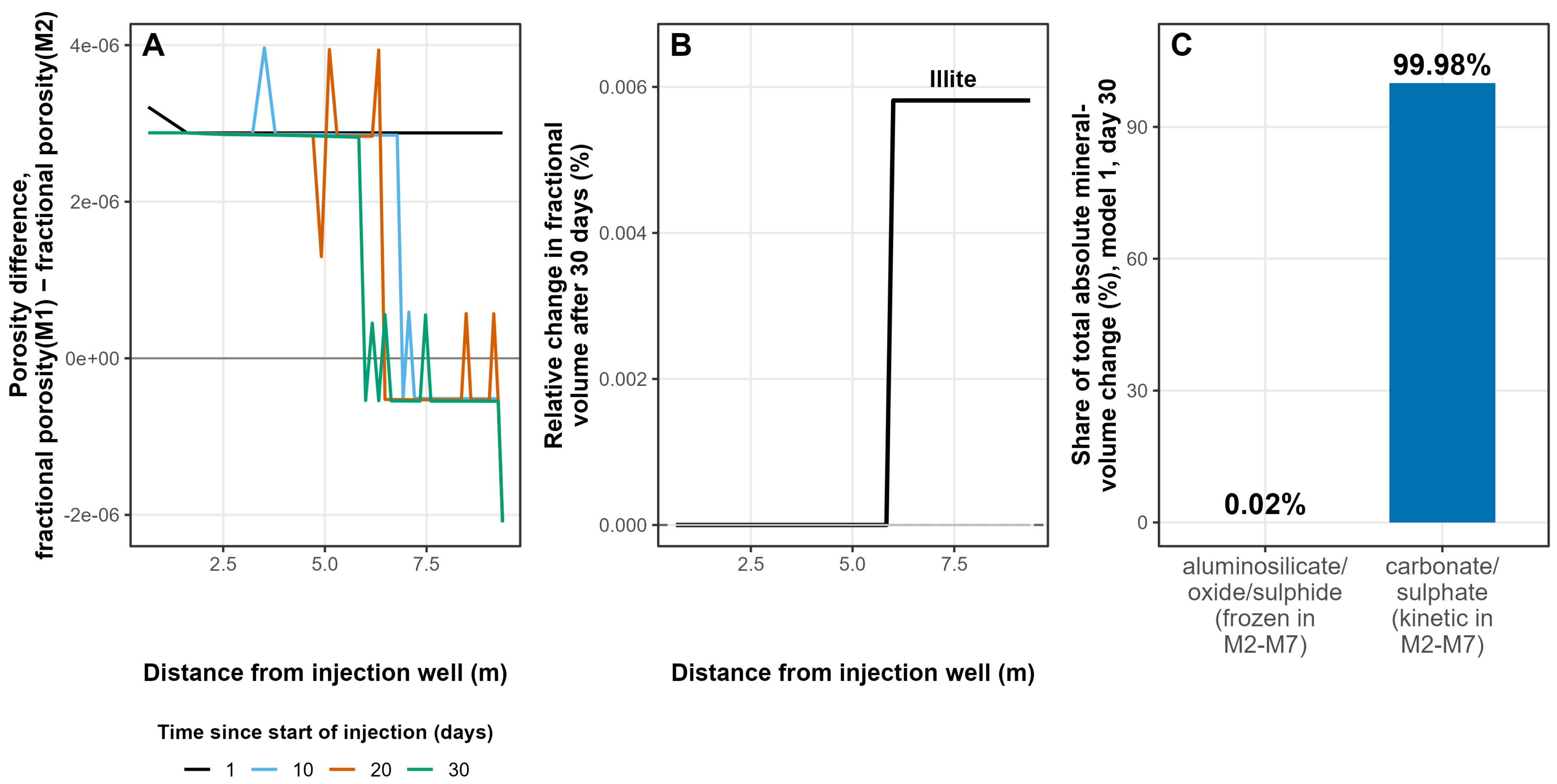
Comparing M1, in which all sixteen minerals react kinetically, with M2, in which quartz, the feldspars, the clays, hematite and pyrite are held inert, shows that this simplification has no material effect on the porosity result. The difference in fractional porosity between the two models is close to zero everywhere, with a maximum absolute discrepancy across every cell and time step of 4 × 10⁻⁶, or 0.002% of a typical porosity value of 0.20 (Figure 6A). Of the eight minerals frozen in M2 but kinetically active in M1, seven show no measurable change in fractional volume over the 30-day simulation. The exception is illite, which grows by a barely detectable 0.006% in relative terms and only in the far-field zone that the injected seawater has not reached; dissolved Al there falls roughly tenfold, from around 1 × 10⁻⁷ to around 1 × 10⁻⁸ mol/kgw, alongside smaller declines in K and Si, consistent with the native formation water slowly re-equilibrating rather than any other mineral converting to illite (Figure 6B). Summing the absolute volume change contributed by every mineral in M1 over the full run shows that the carbonate and sulphate phases account for 99.98% of all mineral-volume changes, while the eight aluminosilicate, oxide and sulphide phases together contribute just 0.02% (Figure 6C). This is the basis for treating those eight minerals as inert in M2 to M14: on the 30-day timescale of a pre-injection seawater test, their reaction kinetics are too slow to influence the porosity and injectivity of the well.
Figure 6.
Testing whether the aluminosilicate, oxide and sulphide minerals can be treated as inert over 30 days (M1 vs. M2). (A) Difference in fractional porosity between the full 16-mineral-kinetics model (M1) and the reduced model that freezes quartz, feldspars, clays, hematite and pyrite (M2). (B) Fractional volume change in each of the eight frozen minerals over 30 days. (C) Share of total mineral-volume change contributed by the carbonate and sulphate minerals against the eight frozen phases.
3.3. Sensitivity to the Injected-Water Temperature Regime
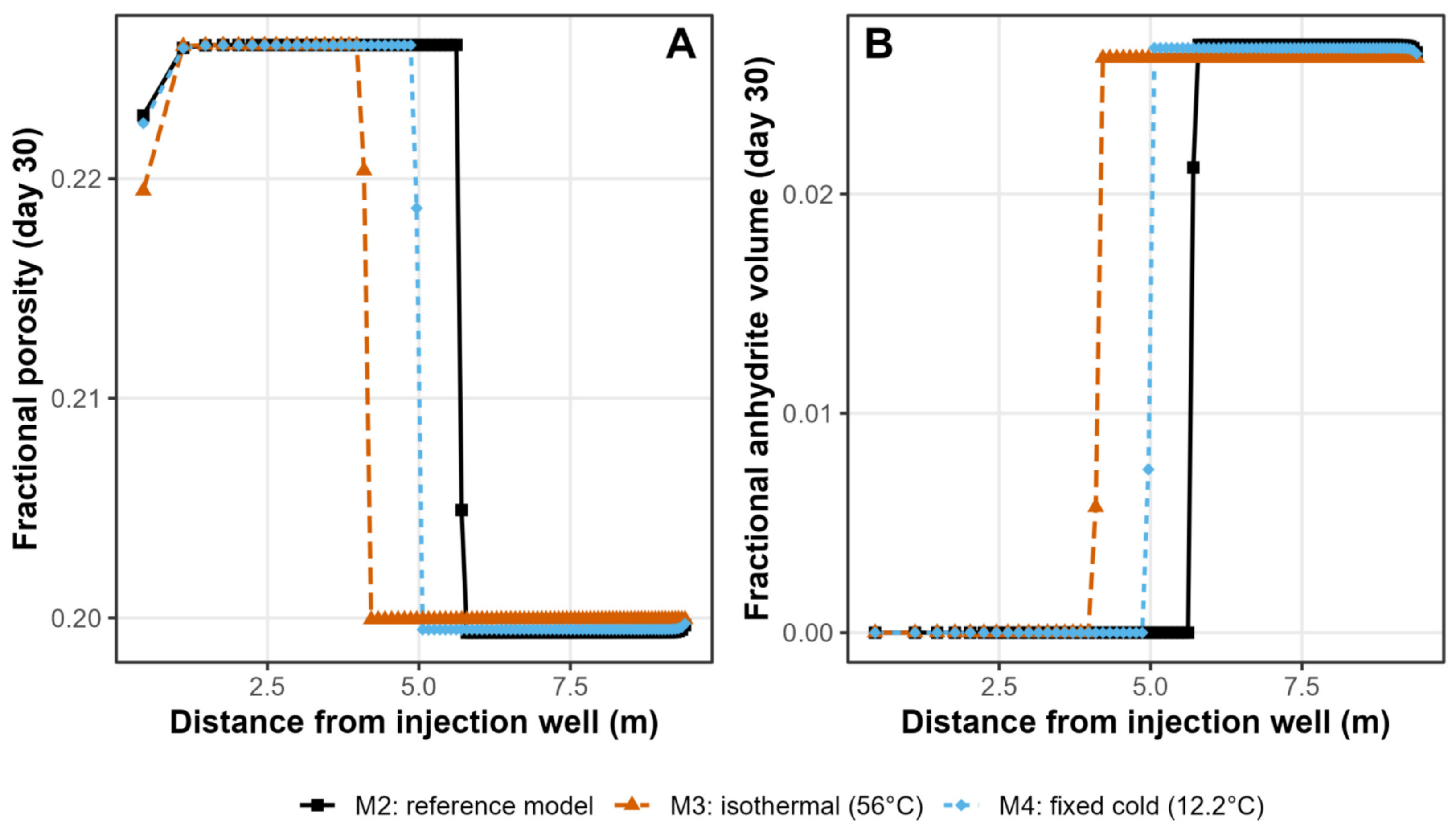
M2 and M4, which apply the same eventual cold temperature but reach it by a staged Ramey schedule (M2) or hold it fixed for the full 30 days (M4), give fronts of 5.71 m and 5.06 m, respectively (Figure 7A,B), a difference of around 11%. The fine detail of how the injected water cools on its way down the well therefore makes a modest difference to the 30-day outcome, smaller than the effect of the eventual cold temperature itself but no longer negligible. In M3, where water is injected at the 56 °C reservoir temperature, the front reaches only 4.21 m, 26% shorter than M2. Ignoring the low temperature of the injected water and simply reacting seawater at the reservoir temperature leave it much closer to anhydrite equilibrium from the outset, so it dissolves less anhydrite for the same injected volume. Wellbore cooling needs to be represented with some care: a single fixed cold temperature is a reasonable approximation of the full Ramey schedule, but not an exact one.
Figure 7.
Sensitivity to the injected-water temperature regime (M2 vs. M3 vs. M4). (A) Fractional porosity versus distance at day 30 for the staged-Ramey-cooling reference case (M2), an isothermal case injected at a full reservoir temperature (56 °C; M3), and a case fixed at the cold Ramey asymptote for the full 30 days (12.2 °C; M4). (B) Corresponding fractional anhydrite volume versus distance.
3.4. Sensitivity to Flow Geometry
Replacing the radial flow geometry of M2 with the one-dimensional, linear flow of the same injected volume, rate and water chemistry (M5) has a large effect on the front position expressed as distance. The radial-model front reaches 5.71 m by day 30, around 63% further than the 3.51 m reached in the linear model (Figure 8A,B). This is the largest difference among the modelling choices tested after the injection rate. It cautions against using a linear reactive-transport column as a direct spatial proxy for flow around an injection well: the distance reached depends on how the injected volume is distributed within the represented geometry. The present comparison does not, however, establish that every linear model will underpredict the reaction-front distance around a real well.
The difference reflects the representation of distance in the two grids, rather than a change in the specified mineral reactions. Both grids are constructed so that every cell holds the same pore volume, but the radial grid achieves this with widths that decrease outwards, from 0.90 m beside the wellbore to 0.053 m at the outer boundary, a 17-fold range. The linear grid uses a fixed width of 0.105 m throughout (Figure 9A). Consequently, the first ten cells span 3.07 m in the radial grid but only 1.05 m in the linear grid (Figure 9B). This difference in the distance represented by the cells contributes directly to the separation of the fronts in Figure 8. Temperature and near-conservative chloride show a similar pattern: at day 1, the thermal front reaches approximately 4 m in the radial grid and 1.8 m in the linear grid (Figure 9C), while the Cl− mixing zones extend over approximately 6.2–7.7 m and 4.2–6.2 m, respectively (Figure 9D). Their separation indicates that the effect is not confined to the anhydrite reaction. In both grids, the thermal and chloride fronts lie well ahead of the anhydrite-buffered reaction front, which has reached only about 1.1 m (radial) and 0.16 m (linear) by day 1.
Table 4.
List of all PHREEQC simulations and the varying grid types, injection rates, approach to water injection temperatures, minerals reacted and thermodynamic database employed (F.W: Bunter formation water).
Figure 8.
Sensitivity to flow geometry (M2 radial vs. M5 linear). (A) Fractional porosity versus distance at day 30. (B) Corresponding fractional anhydrite volume versus distance.
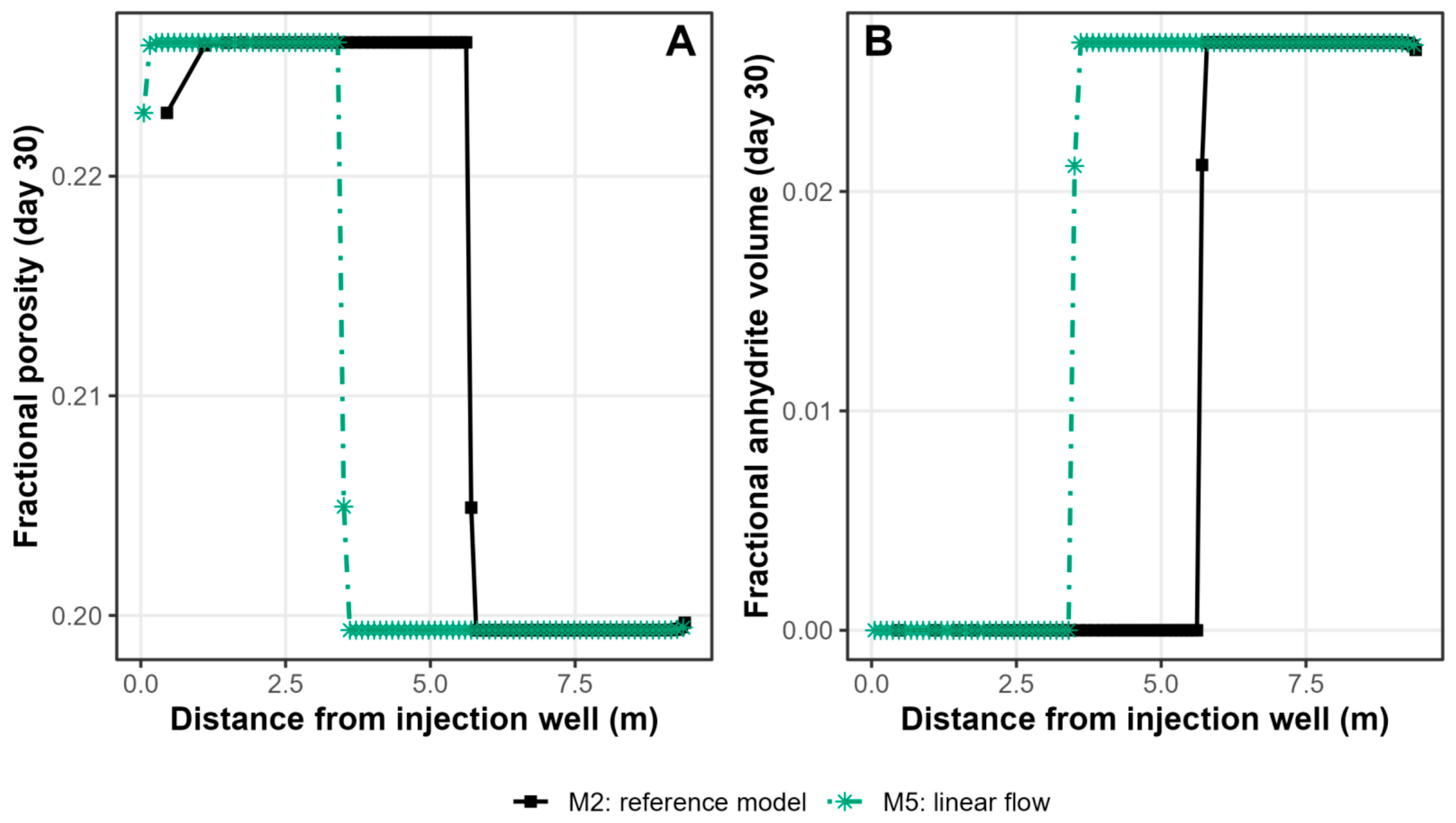
Figure 9.
Origin of the geometry sensitivity in Figure 8. (A) Cell width versus distance for the radial and linear grids. (B) Cumulative distance swept per cell for each grid. (C) Temperature versus distance at day 1. (D) Dissolved Cl− versus distance at day 1.
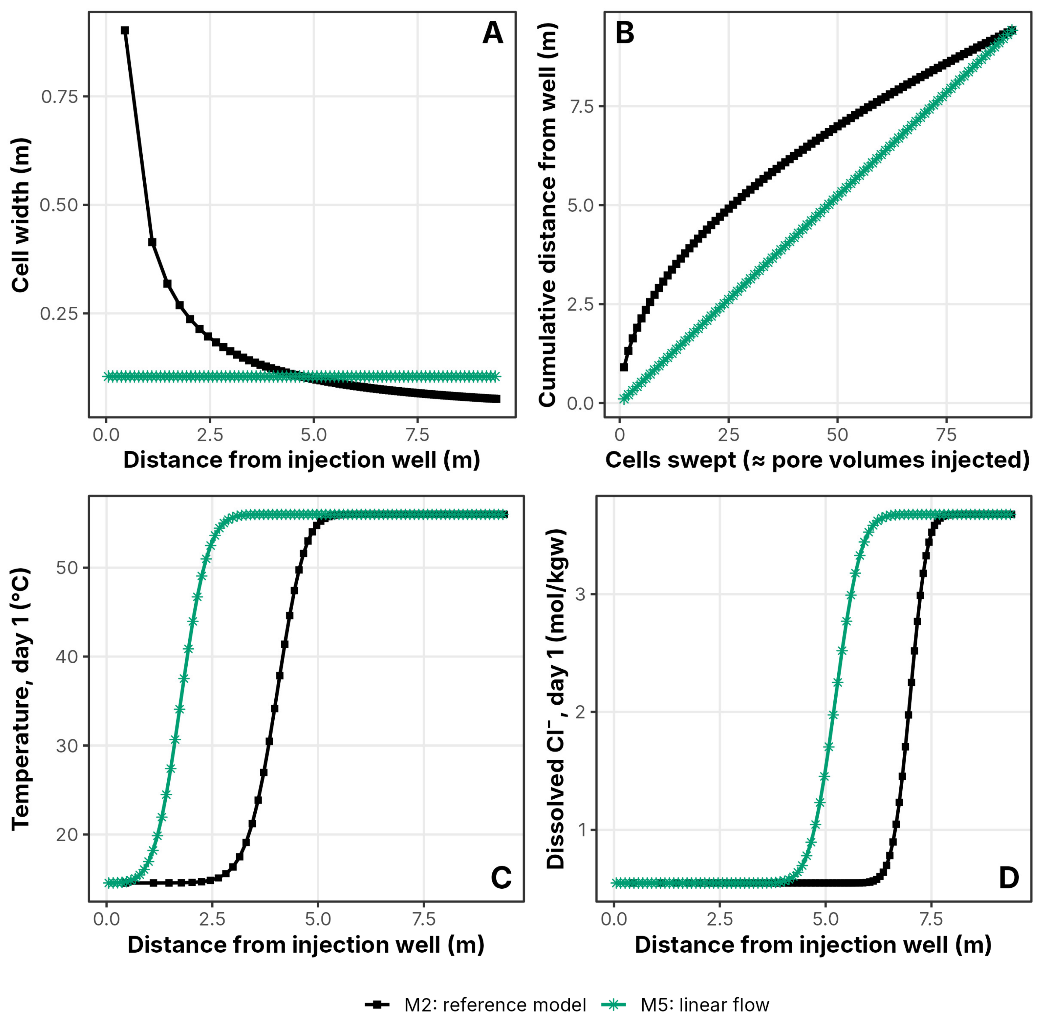
In radial flow, the area through which water passes increases with distance from the well; at a fixed injection rate, the flux per unit area and interstitial velocity therefore decrease approximately as 1/r. A linear column of a fixed cross-section instead has a constant velocity. In the particular grids used here, equal cell pore volumes mean that the injected water passes through the same number of cells in a given time in either model, but those cells span different physical distances. The longer front distance in M2 is therefore consistent with the radial geometry represented by its grid. Because the linear column was given the same pore volume per cell as the radial grid, the comparison is volume-matched and does not depend on an arbitrary choice of cross-section, nor does it depend on cell size (Section 3.5).
3.5. Sensitivity to Grid Discretisation
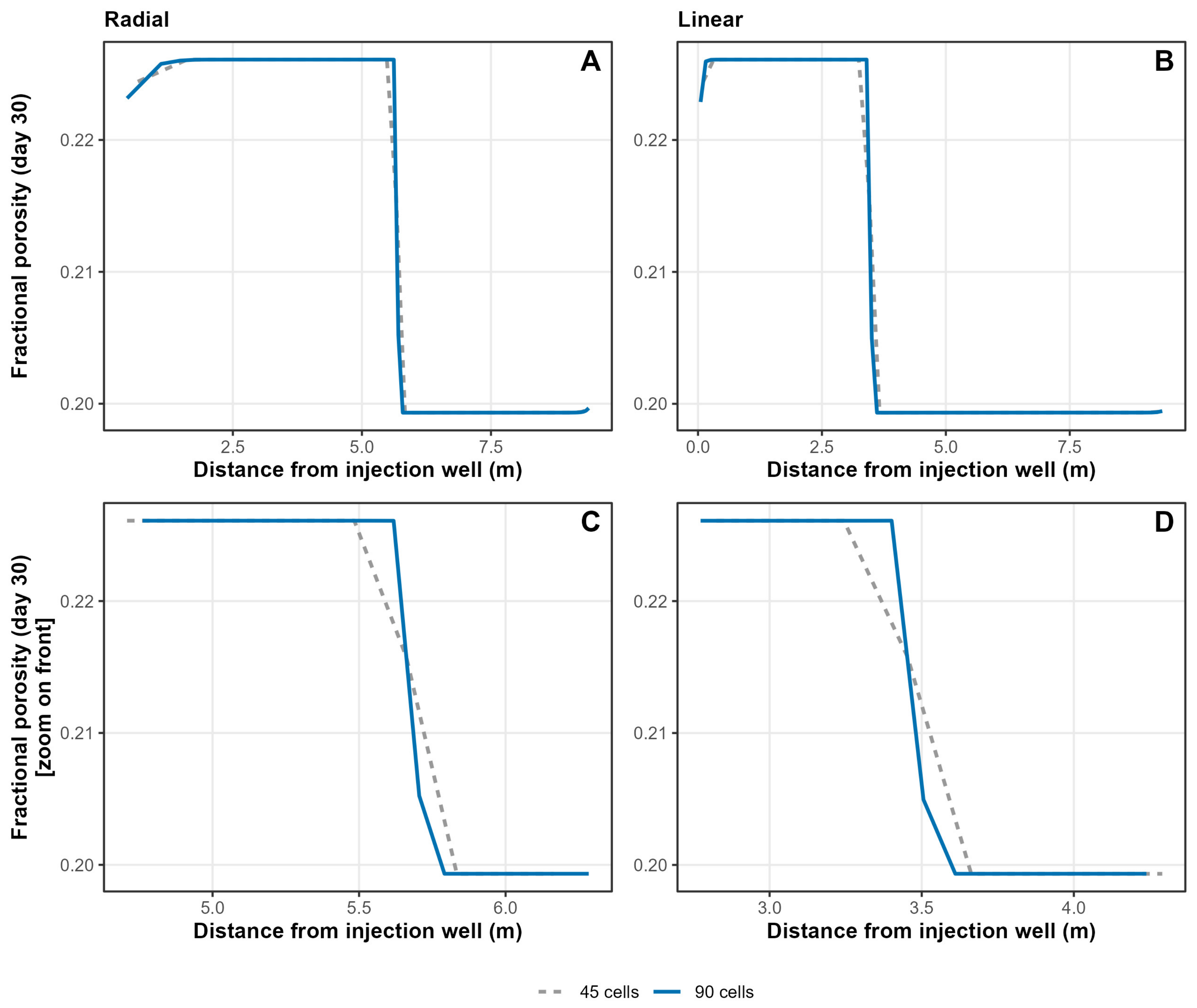
A grid-refinement test compared 90-cell and 45-cell versions of the radial (M2) and linear (M5) models over an unchanged domain (radial 0.108–9.53 m; linear 9.42 m), so that only the cell size changed. Refining the grid shifts the day-30 front by 2.2% (radial) and 4.3% (linear), in each case by less than the width of one 45-cell grid cell at the front (0.17 m and 0.21 m; Figure 10), so the 5.71 m versus 3.51 m difference between the radial and linear models (Section 3.4) reflects the flow geometry itself rather than the chosen cell dimensions. The 30-day increase in dolomite next to the well (0.108–1.42 m), the main zone of mineral precipitation, is 2.45% on both grids (on the 90-cell grid, the mean of the two cells spanning that interval); the use of the finer 90-cell grid concentrates this growth in its innermost cell (4.67%).
Figure 10.
Effect of grid discretisation on the day-30 porosity profile, comparing a 45-cell grid with the 90-cell grid used for all other models (M2 radial and M5 linear, both at 10,000 bbl/d with staged Ramey cooling). (A) Fractional porosity versus distance, radial grid, full domain. (B) Fractional porosity versus distance, linear grid, full domain. (C) Radial profile, zoomed on the front. (D) Linear profile, zoomed on the front.
3.6. Sensitivity to Injection Rate
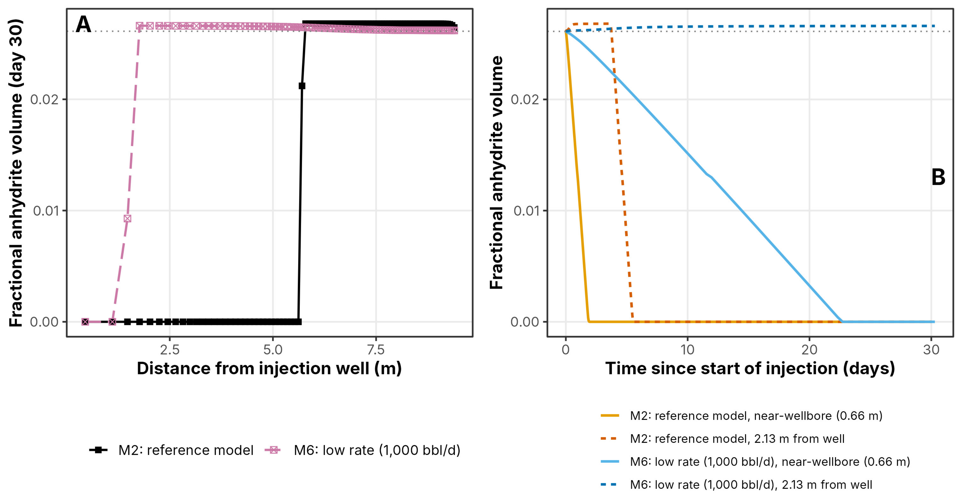
Lowering the injection rate tenfold, from 10,000 bbl/d (M2) to 1000 bbl/d (M6), produces the largest single sensitivity of any variable tested. M2 reaches its maximum near-well porosity within about two days and advances its reaction front to 5.71 m by day 30, whereas M6 takes about twelve times as long (about 23 days) to reach the same near-well porosity plateau, and its front reaches only 1.77 m by day 30 (Figure 11A,B). These are the responses expected from the tenfold smaller volume of seawater injected: in radial flow, the swept volume scales with the square of the radius, so a tenfold smaller volume shortens the front by a factor of about √10 (Section 4.3). The warmer water injected at 1000 bbl/d (approximately 26–37 °C over the Ramey stages, against approximately 12–15 °C at 10,000 bbl/d) does not offset the lower flux: because anhydrite solubility decreases with temperature, it slightly reduces the dissolution capacity of the water, as the isothermal comparison of M10 with M6 confirms (Section 3.8). Anhydrite is completely removed behind the front in both models, with only a small excess, about 2.6%, over the background anhydrite content at the leading edge (Figure 12).
Figure 11.
Sensitivity to injection rate (M2 vs. M6, 10,000 vs. 1000 bbl/d). (A) Fractional porosity versus distance at day 30. (B) Fractional porosity versus time at 0.66 m and 2.13 m from the well.
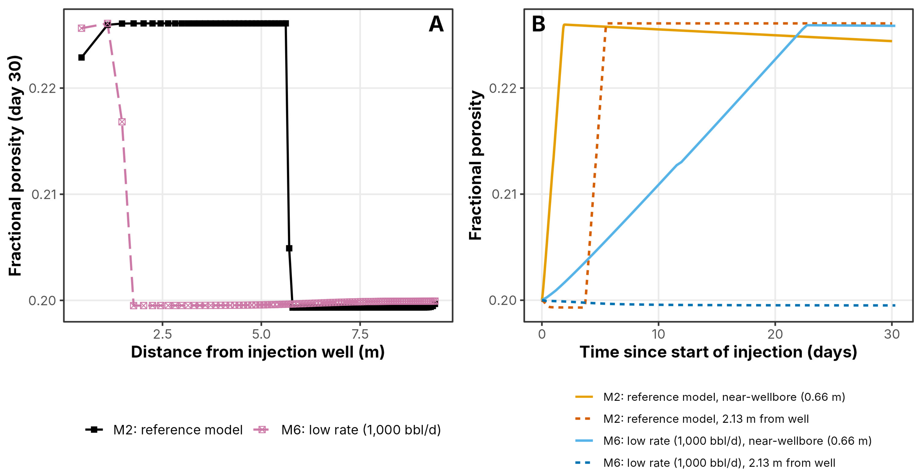
Figure 12.
Anhydrite at and behind the reaction front at the two injection rates (M2 and M6). (A) Fractional anhydrite volume versus distance at day 30, M2 and M6. (B) Fractional anhydrite volume versus time at the same two positions as Figure 11B.
3.7. Sensitivity to the Thermodynamic Database
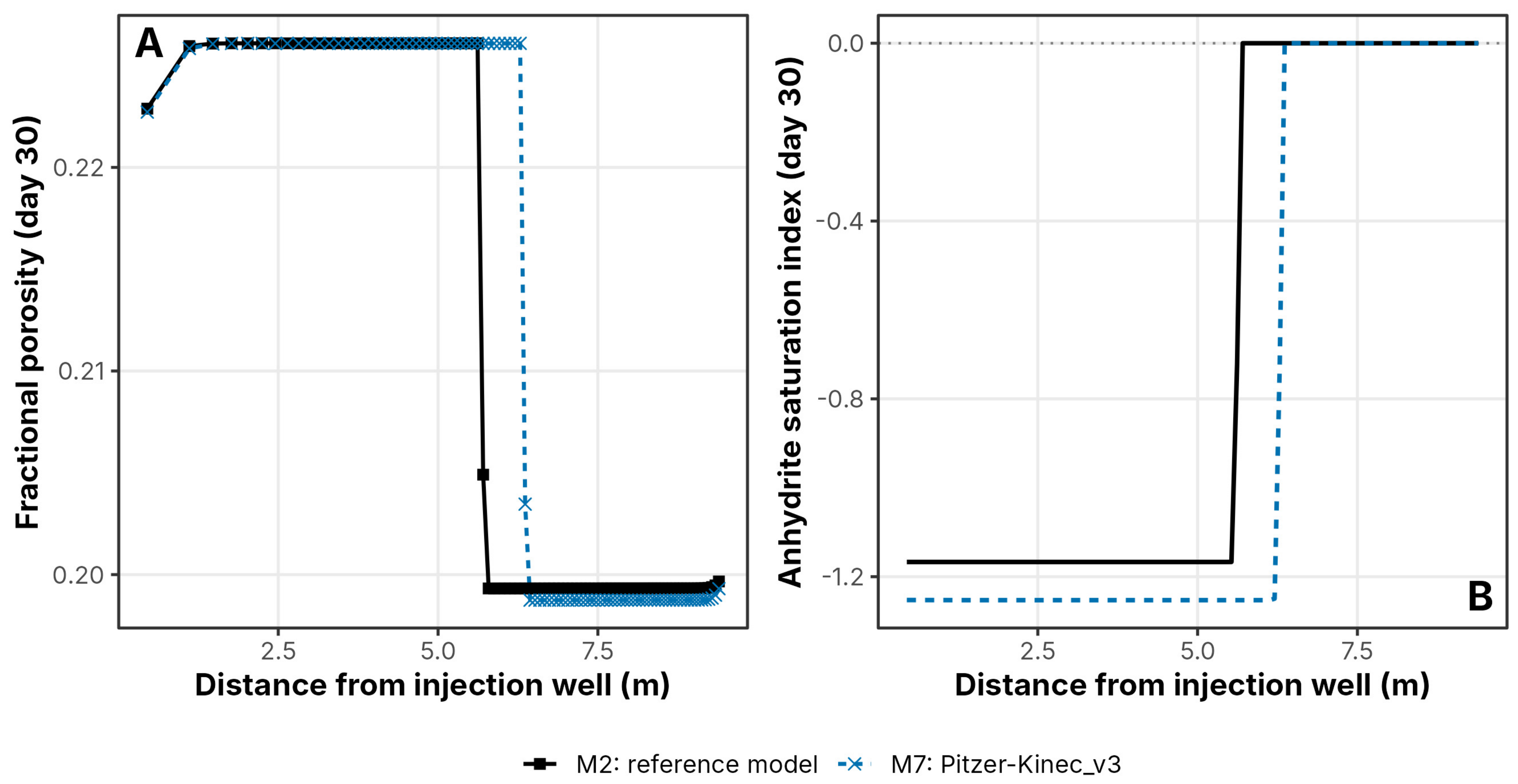
Replacing Kinec_v3′s native extended Debye–Hückel activity model (M2) with the Pitzer ion-interaction model (M7) gives a modestly longer reaction front, 6.36 m against 5.71 m, a 12% difference and one of the smallest of the sensitivities examined in this study, though not negligible (Figure 13A). The difference arises in seawater-dominated water, not in the 4 mol/kgw formation brine, which is displaced from the near-well domain within about two days; at day 30, the water on both sides of the front has an ionic strength of about 0.6–1.0 mol/kgw. In that water, the two activity models give different activities of Ca2+ and SO42− and therefore different anhydrite saturation states and dissolution capacities. Because the swept volume scales with the square of the front radius, the 12% longer Pitzer front corresponds to about 24% more anhydrite dissolved per kilogram of seawater, so the extended Debye–Hückel reference case underestimates, rather than overestimates, the predicted enhancement. Figure 13B compares the anhydrite saturation index under each model. Free-ion activity coefficients are not compared directly, because the ion-association model treats CaSO40, MgSO40 and NaSO4− as explicit species, whereas the Pitzer model includes these interactions within the activity coefficients [52].
Figure 13.
Sensitivity to the thermodynamic database (M2, Kinec_v3 with extended Debye–Hückel, vs. M7, Pitzer-Kinec_v3). (A) Fractional porosity versus distance at day 30. (B) Comparison of anhydrite saturations at day 30 as a function of distance.
3.8. Factorial Analysis
The comparisons above vary the injection rate, flow geometry and injected-water temperature regime one at a time against the M2 reference case (Figure 7, Figure 8, Figure 11 and Figure 13), which is sufficient to rank their individual importance but cannot show whether the three variables act independently or interact with one another. To test this directly, the design was completed into a full 2 × 2 × 3 factorial: seven further models (M8–M14) were added to the five already available (M2–M6), giving every combination of injection rates (10,000 or 1000 bbl/d), flow geometry (radial or linear) and temperature regimes (staged Ramey cooling, isothermal at 56 °C or fixed-cold) its own dedicated simulation, twelve models in total. Figure 14, Figure 15 and Figure 16 report the resulting porosity, anhydrite and dolomite fields at day 30 across the full design.
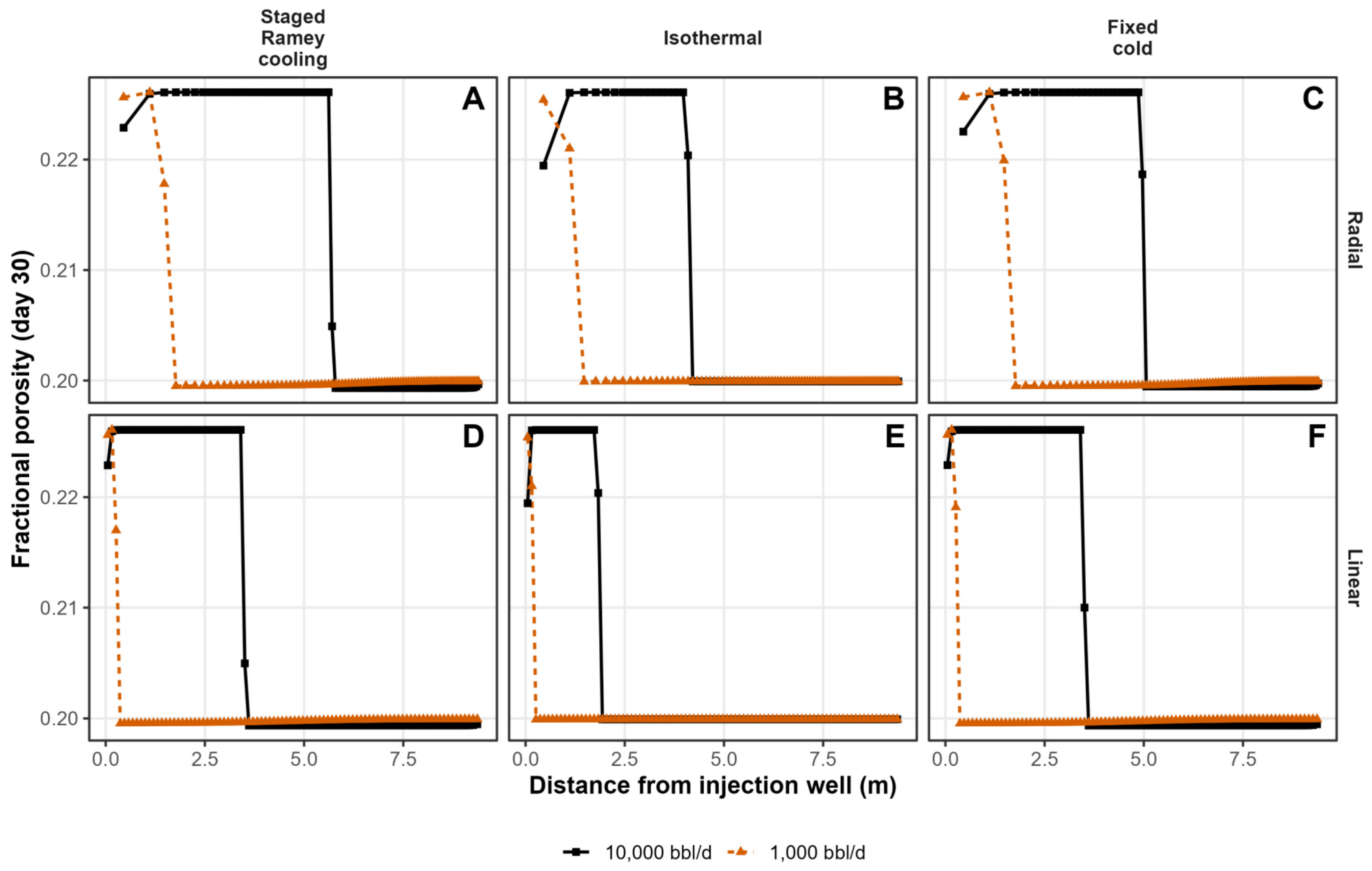
Every one of the twelve combinations shows the same qualitative pattern already established for the reference case, an elevated porosity plateau near the well decaying at a sharp front to the initial value of 0.20 (Figure 14, panels A–F), confirming that the behaviour does not depend on the parameter combination chosen for M1 and M2. What differs systematically across the grid is how far that front has advanced by day 30. Comparing rows shows the radial fronts (A–C) consistently outrunning their linear counterparts (D–F) at a matched rate and regime, and comparing columns shows the staged-Ramey and fixed-cold panels (A, C, D, F) consistently outrunning the isothermal panels (B, E) at both injection rates.
Figure 14.
Full factorial sensitivity of the porosity to injection rate, flow geometry and injected-water temperature regime (Table 4). Each panel shows fractional porosity versus distance at day 30 for both injection rates (10,000 bbl/d, solid black; 1000 bbl/d, dashed orange) under one combination of flow geometry (rows) and temperature regime (columns). (A) Radial, staged Ramey cooling (M2, M6). (B) Radial, isothermal at 56 °C (M3, M10). (C) Radial, fixed-cold (M4, M11). (D) Linear, staged Ramey cooling (M5, M12). (E) Linear, isothermal at 56 °C (M8, M13). (F) Linear, fixed-cold (M9, M14).
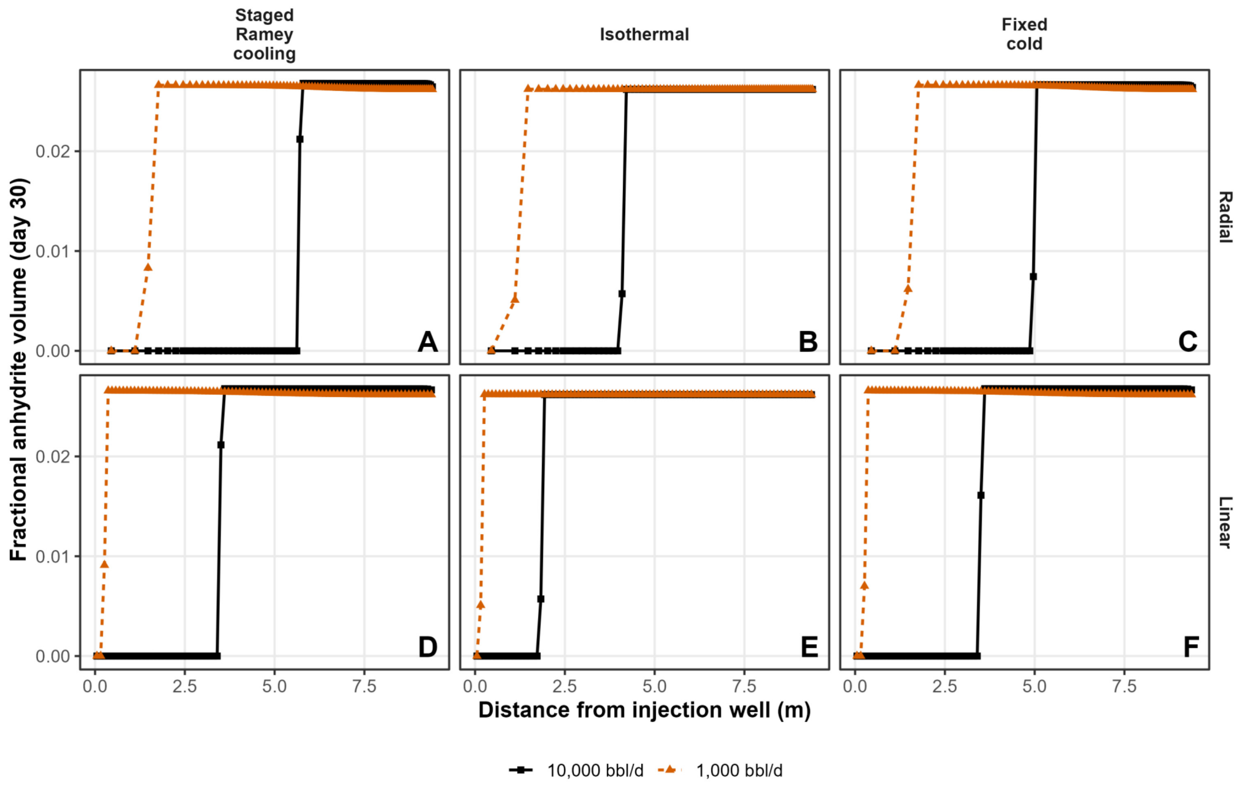
The anhydrite dissolution front position can be compared quantitatively across all twelve models (Figure 15). Averaged over the three temperature regimes, raising the injection rate from 1000 to 10,000 bbl/d advances the front by 2.99 m; averaged over both rates, replacing linear with radial flow advances it by a further 1.67 m; and averaged over both rates and both geometries, replacing staged Ramey cooling with isothermal injection at 56 °C retards it by 0.87 m, while replacing it with a fixed-cold schedule changes it by a more modest 0.16 m on average, consistent with the M2–M4 difference identified in Figure 7. These three effects are not perfectly additive: all three are largest in the radial, high-rate corner of the design, where the front is longest and best resolved by the grid, and they compress toward the linear, low-rate corner, where the front in the most retarded cases (M13, M14) is confined to the first two or three grid cells and cannot be resolved further. This is a consequence of grid resolution rather than a change in the underlying chemistry, and the ranking itself, injection rate first, flow geometry second and temperature regime third, holds throughout the factorial design just as it does in the single-comparison case.
Figure 15.
Fractional anhydrite volume versus distance at day 30 for the same full factorial design as Figure 14 (M2, M3, M4, M5, M6, M8–M14). Panel layout and model assignment follow Figure 14: (A) Radial, staged Ramey cooling. (B) Radial, isothermal at 56 °C. (C) Radial, fixed-cold. (D) Linear, staged Ramey cooling. (E) Linear, isothermal at 56 °C. (F) Linear, fixed-cold. Solid black lines, 10,000 bbl/d; dashed orange lines, 1000 bbl/d.
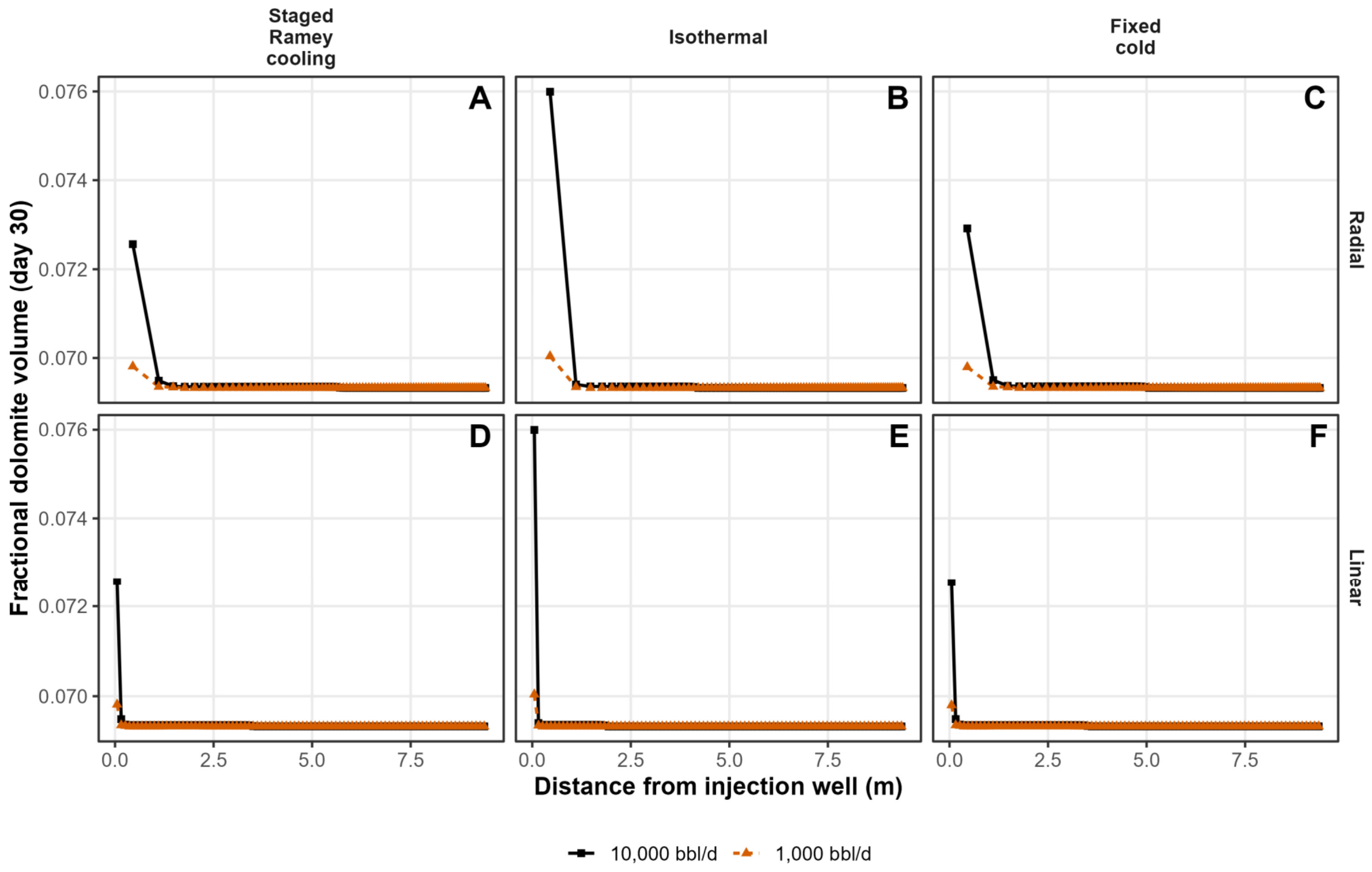
Dolomite shows a different and, in one respect opposite, sensitivity (Figure 16). The 30-day wellbore dolomite increase ranges from as little as 0.68% (M11, M14) to as much as 9.62% (M8) across the twelve models, and in every one of the four rate-geometry combinations tested, the isothermal case shows a higher dolomite increase than its staged-Ramey or fixed-cold counterpart at the same rate and geometry, roughly doubling it at the higher injection rate (9.62% for isothermal M8 against 4.67% for staged M5 and 4.64% for fixed-cold M9, at 10,000 bbl/d in linear flow) and increasing it by around one and a half times at the lower rate. This is the reverse of the pattern seen for the anhydrite front, which isothermal injection shortens rather than lengthens. The two responses are controlled by different mechanisms: the anhydrite front’s advance is governed by the undersaturation that the injected fluid carries, which is greater in cooler water because anhydrite solubility increases as the temperature falls. Dolomite growth, in contrast, is not limited by the undersaturation of the fluid but by the kinetic rate law assigned in Kinec_v3, whose rate constant increases with temperature following an Arrhenius relationship. The isothermal schedule holds the near-well zone at the full 56 °C reservoir temperature for the entire 30-day simulation, whereas the staged-Ramey and fixed-cold schedules keep it close to the cold Ramey asymptote (12–15 °C at 10,000 bbl/d) for almost the whole period; sustaining the higher temperature for longer therefore drives faster dolomite precipitation throughout the isothermal case, producing a higher 30-day dolomite increase than its cooler counterparts at a matched rate and geometry. This is consistent with Figure 16: cell 1′s dolomite volume reaches about 0.0760 in the isothermal columns (B, E) at 10,000 bbl/d, against 0.0725–0.0729 in the staged-Ramey and fixed-cold columns (A, C, D, F), which track each other closely, consistent with both schedules spending nearly all 30 days at the same cold asymptote, regardless of the modest front-position sensitivity to cooling-schedule detail noted for the anhydrite front in Section 3.3.
Figure 16.
Fractional dolomite volume versus distance at day 30 for the same full factorial design as Figure 14 and Figure 15 (M2, M3, M4, M5, M6, M8–M14), showing dolomite precipitation near the wellbore across all twelve models. Panel layout, model assignment and line coding follow Figure 14 and Figure 15: (A) Radial, staged Ramey cooling. (B) Radial, isothermal at 56 °C. (C) Radial, fixed-cold. (D) Linear, staged Ramey cooling. (E) Linear, isothermal at 56 °C. (F) Linear, fixed-cold.
3.9. Sensitivity to the Surface Area Inputs for Anhydrite and Dolomite
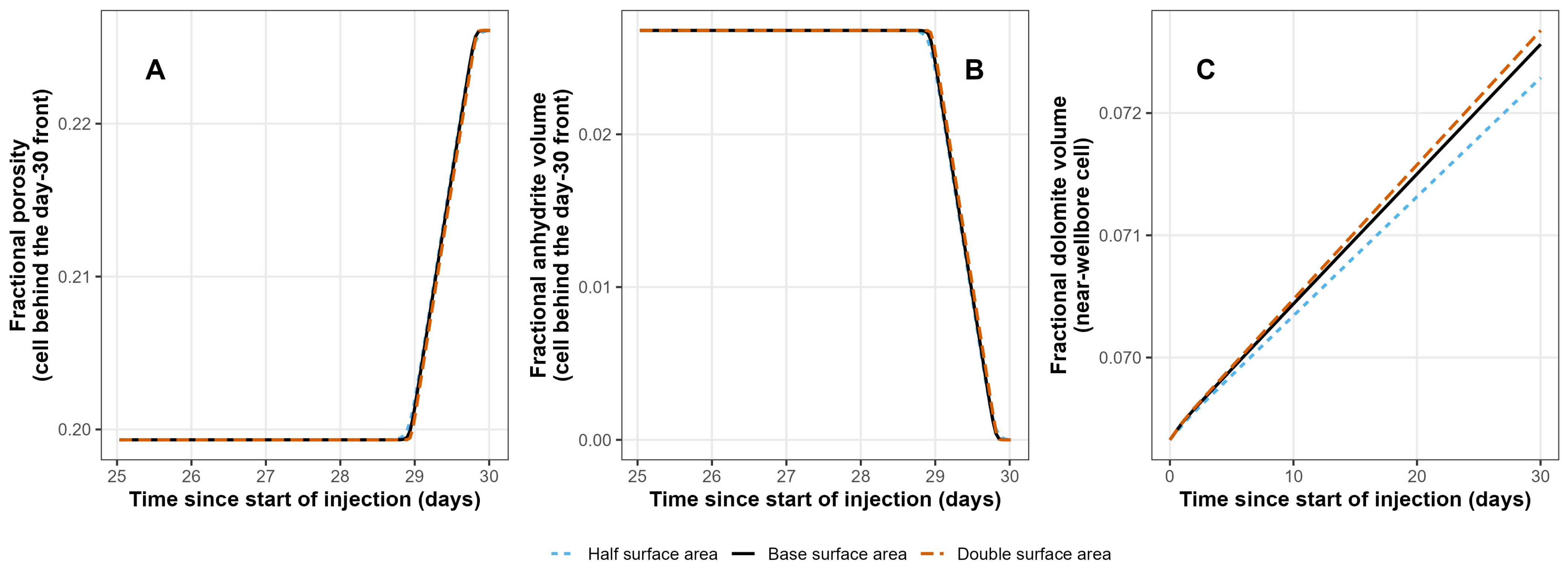
Two further M2 runs tested the sensitivity of this result to the reactive surface area assigned to anhydrite and dolomite in the kinetics block, doubling and halving the value used throughout the rest of this study (Table 2). The day-30 porosity and anhydrite front position are unaffected by this parameter, remaining at 5.71 m in all three cases (Figure 17), consistent with front advance being governed by the mass balance of the injected fluid rather than by the dissolution rate once the fluid is undersaturated with respect to anhydrite. Wellbore dolomite growth, which is kinetically rather than transport-limited, responds more directly to the surface area: the 30-day increase ranges from 4.27% at the lower value to 4.83% at the higher, against 4.67% for the reference case (Figure 17B and Figure 18C). Time series at the cell immediately behind the front (Figure 18A,B) show this front-position insensitivity holding throughout the final days of injection, not only at day 30. The front is insensitive because anhydrite dissolution is fast relative to advection (a high Damköhler number), so the front position is set by local equilibrium rather than by the rate law [53].
Figure 17.
Effect of halving and doubling the anhydrite and dolomite reactive surface area on the day-30 spatial profile. (A) Fractional porosity and (B) fractional dolomite volume versus distance, full domain. (C) Porosity and (D) anhydrite volume versus distance, zoomed on the front.
3.10. Sensitivity to the Assumed Absence of Halite and Elevated Aqueous Sulphate
Halite has been reported in XRD data from the Bunter Sandstone Formation [7,35,54] and has been shown to be a genuine diagenetic mineral in some studies [36]. Earlier, it was suggested that the halite may be an artefact of saline formation water evaporation as opposed to a real feature of the sandstone because the formation water is nowhere near saturation with halite. Halite dissolution kinetics are extremely rapid [18,55]. A repeat of any of the models of seawater injection with a 0.05 fraction of halite leads to an automatic 0.05 fractional increase in porosity throughout the whole grid within 1 day. It is not that the presence of halite does not matter, rather it cannot persist as a mineral under the modelled water conditions as a 0.05 fraction of the formation in the reported formation water because the water is undersaturated.
Conversely, using a lower reported aqueous sulphate concentration of 385 mg/kgw [35], instead of the value of 3903 mg/kgw (Table 3: the result of pre-equilibration of the water with anhydrite), makes a limited difference to the porosity evolution. Near the outer model boundary at 9.53 m from the wellbore, the low-sulphate case sits about 0.00037 fractional-porosity units above the high-sulphate case (0.20001 vs. 0.19964; roughly a 0.18% relative increase for the low-sulphate case). This is a small difference, but it is not noise. Significantly, the difference in porosity does not grow with time once it is established. In the near-wellbore zone, there is no influence of the initial formation water composition by day 2.5 out of 30 since the water allowing the dissolution of anhydrite is injected seawater in both cases.
4. Discussion
This study was designed to address whether seawater injection into a sandstone, in this case the Lower Triassic Bunter Sandstone Formation in the Southern North Sea Basin, UK, is likely to damage, improve or leave largely unchanged the injectivity of a well, ahead of CO2 injection. Here, the results presented in Figure 3, Figure 4, Figure 5, Figure 6, Figure 7, Figure 8, Figure 9, Figure 10, Figure 11, Figure 12, Figure 13, Figure 14, Figure 15, Figure 16, Figure 17 and Figure 18 are collectively interpreted and compared to the wider literature on seawater and brine injection and the simplifications employed in the models are assessed for validity.
Figure 18.
Effect of halving and doubling the anhydrite and dolomite reactive surface area on the time evolution of the result. (A) Fractional porosity and (B) fractional anhydrite volume at the cell immediately behind the day-30 front, days 25–30. (C) Fractional dolomite volume at the near-wellbore cell over the full 30-day injection period.
4.1. Does Seawater Injection Damage, Improve or Leave Injectivity Unchanged?
Within the 30-day, near-well window examined here, the model predicts an increase in porosity from 0.200 to approximately 0.226 in the zone swept by seawater (Figure 3). The reactive-transport calculation does not calculate permeability or well injectivity. As a first-order estimate of the likely hydraulic consequence, the porosity change was translated to a local intrinsic-permeability change using a Kozeny–Carman-type relationship [56], assuming unchanged grain size, tortuosity, pore connectivity and specific surface area where ϕ0 and ϕ1 are the initial and final porosity values and k0 and k1 are the initial and final permeability values:
The substitution of ϕ0 = 0.200 and ϕ1 = 0.226 gives k1/k0 = 1.54, equivalent to an approximately 54% local increase in intrinsic permeability. Applying this multiplier to the 271 mD mean horizontal core permeability reported for Endurance [13] would give a permeability of approximately 418 mD.
As an independent consistency check based on the Kozeny–Carman estimate, rather than a validation of the reacted rock, two published porosity–permeability relationships for the Bunter Sandstone can be compared: a 2016 report proposed a porosity–permeability algorithm that suggested that a porosity of 0.200 should equate to a permeability of 294 mD and a porosity of 0.226 should equate to a permeability of 574 mD [57], representing a 95% increase. A more recently published porosity–permeability relationship for the cleaner sandstone in the Bunter Sandstone Formation suggested that a porosity of 0.200 should equate to a permeability of 90 mD and a porosity of 0.226 should equate to a permeability of 204 mD [58], equal to a 127% increase.
These increases in permeability are illustrative rather than a site-wide prediction because measured permeability at Endurance spans a wide range, and the permeability response to cement dissolution depends on the connectivity and geometry of the newly opened pore space. This bias could act in either direction. Anhydrite in the Bunter Sandstone is a pore-filling cement [7,36], so its removal could reopen pore throats and raise permeability by more than the Kozeny–Carman relationship implies; conversely, poorly connected secondary pores, or fines mobilised as the cement dissolves, would raise it by less. The three multipliers (1.54, 1.95 and 2.27) therefore need to be treated as a range of plausible responses, and the injectivity estimate below uses the smallest.
The possible consequence for aqueous well injectivity was estimated using a two-zone, radial-flow representation of a near-well region of enhanced permeability [59]. For an altered zone extending from wellbore radius rw to radius ra, surrounded by unaltered rock to an effective outer radius re, J0 and J1 are the initial and final injectivity values; then, the injectivity-index ratio is as follows:
Using k1/k0 = 1.54, from the Kozeny–Carman-type porosity–permeability relationship, discussed previously, and m, the 1.48–6.36 m day-30 reaction-front range spanned by the radial-flow cases and illustrative effective outer radii of 100–1000 m gives an aqueous injectivity-index increase of approximately 11–27%; the outer radii are sensitivity bounds, not calibrated radii of investigation for the Endurance test. Two minor zones of porosity loss reduce this only slightly: dolomite growth in the cell next to the well, which lowers porosity from 0.226 to about 0.223 by day 30 (Figure 4B and Figure 11B), and anhydrite precipitation ahead of the front, where cold, anhydrite-saturated water is re-warmed (a loss of about 0.0007; Figure 11A and Figure 14). Including both in a multi-zone form of Equation 5 [60] lowers the range to about 10–25%, mostly through the near-well zone, because radial flow gives most weight to the rock nearest the well. This range is an illustrative hydraulic implication of the modelled porosity change, not a measured Endurance injectivity response, and should not be read as a prediction of CO2 injectivity, for which the multiphase flow, relative permeability, completion skin, fines migration and geomechanical response would also need to be represented.
The predicted porosity increase is a geochemical enhancement, not necessarily a net injectivity enhancement. Anhydrite occupies about 2.6% of the bulk rock volume, and its complete removal near the well could release fines, notably authigenic illite (about 6% of bulk volume; Table 2), or reduce the support of detrital grains. The release of fines via a salinity reduction is unlikely, because seawater (ionic strength about 0.7 mol/kgw, with abundant Ca and Mg) is far more saline than the critical salt concentrations typically associated with clay detachment [61]. The mechanical mobilisation of particles freed via cement dissolution and any loss of framework strength cannot however be assessed with a geochemical model. Reactive core-flood experiments using a Bunter Sandstone core and seawater at a bottom-hole temperature are therefore needed to establish the net effect on permeability.
These estimates rest on simplifications that a real well test would not share: a single homogeneous layer of constant thickness, single-phase water flow at a constant rate, an outer model boundary at 9.5 m and dispersivity tied to cell size. Layering would distribute the injected volume unevenly; because the reacted radius scales with the square root of the volume injected per unit thickness, a high-permeability layer receiving more water would develop a longer reacted zone, but the direction of reaction, which is set by the undersaturation of the injected water, would not change. Completion skin, fines migration, pressure limits and geomechanical change lie outside the scope of a geochemical model. Measured bottom-hole temperatures and pressures from an injection test would provide the best calibration for an operational assessment.
The porosity increase is driven by the dissolution of anhydrite rather than by any of the other fifteen minerals present (Figure 4), and the accompanying pH and saturation-index response shows that this is a self-consistent geochemical reaction rather than a numerical artefact (Figure 5). Field evidence for the fluid-rock reaction proceeding fast enough to matter on a production timescale exists: it has been documented that produced-water chemistry from the Miller Field, North Sea, departed systematically from the simple mixing of seawater and formation water within around 600 days of seawater breakthrough [62].
4.2. Oilfield and Analogue Experience of Seawater and Brine Injection
Anhydrite has retrograde solubility, so whether injected seawater dissolves or precipitates it depends strongly on the temperature; the studies discussed in this section are summarised in Table 5. McCartney [63], reviewing predicted sulphate mineral deposition across 81 fields on the UK and Norwegian continental shelves, found that the heating of injected seawater to reservoir temperature only drives anhydrite deposition above a threshold of roughly 120 to 129 °C and that deposition from mixing with formation water more generally requires either calcium-rich formation water (above roughly 6000 mg/L Ca) or a reservoir at the higher end of that temperature range. Al-Behadili and Mackay [64], modelling a comparable sandstone reservoir containing the carbonate and sulphate minerals, found this switch: anhydrite dissolved when the injected seawater stayed cold, but precipitated once it reached the reservoir’s full temperature of 136 °C with a full-sulphate seawater. The dissolution behaviour found throughout this study is therefore consistent with, rather than contrary to, the pattern established elsewhere for warmer reservoirs, and the two apparently opposite outcomes to research question 1, injectivity damage and injectivity improvement, are best understood as the same mineral reaction occurring on opposite sides of a temperature threshold rather than as two unrelated behaviours. Hajiabadi et al.’s [65] review of hydro-physical, chemical and geomechanical controls on CO2-storage well injectivity reaches the same general conclusion from a wider survey of the CO2 storage literature: a geochemical reaction can either impair or enhance injectivity, and which of the two occurs is case-specific rather than a fixed property of injecting an incompatible water.
In North Sea oilfields, the main scale minerals are barite and celestite rather than anhydrite. Osborne, Ravenscroft and McCracken [66] and Yuan, Todd and Sorbie [67] both modelled the incompatibility between sulphate-rich seawater and the barium- and strontium-rich formation waters typical of many North Sea oil reservoirs and found that the barite, strontium sulphate and calcium sulphate scale form is in sequence as the mixed water becomes progressively more seawater-dominated, with barite forming first, at low seawater fractions, and calcium sulphate only once the mixture is almost entirely seawater. Fu et al. [16], modelling the Miller Field with a one-dimensional PHREEQC transport model, found strontium-bearing barite precipitating along the flow path towards the production well while calcite and quartz dissolved close to the injection well. Barite and celestite are included among the sixteen kinetic minerals in the full-kinetics model reported here (Figure 6C), yet neither contributes measurably to the result. The Bunter Sandstone formation water used in this study (Table 3) carries a low barium and only a modest strontium concentration, which is the most likely explanation; this is a feature of the specific water compositions used here rather than a general property of the modelling approach.
Table 5.
Comparative summary of the oilfield and analogue seawater or brine injection studies discussed in this section, set against the Bunter Sandstone model reported in this study.
Al-Behadili and Mackay [64] established the temperature control based on anhydrite behaviour discussed above under research question 1. Fu et al.’s [16] one-dimensional PHREEQC model of the Miller Field is the closest methodological precedent to the approach used in this study: a reactive transport model, rather than a batch or flash calculation, applied to a real seawater-injected sandstone reservoir, and one that likewise finds near-well mineral dissolution and porosity enhancement occurring alongside far-field precipitation, in their case, reaching near-equilibrium within under two years.
Kermani, Bonto and Nick [68] modelled produced-water reinjection in the Danish North Sea with PHREEQC, the same modelling tool as this study, and identified chemical treatments capable of restoring injectivity once iron sulphides and carbonate and sulphate mineral scales had already impaired injectivity. Tranter et al. [70], modelling a barite-driven injectivity decline during geothermal brine reinjection in Germany, found major injectivity losses over ten years depending on reservoir salinity and temperature, showing that the same balance between precipitation and dissolution applies to geothermal reinjection.
Across Table 5, whether sulphate minerals dissolve or precipitate depends on the temperature and formation-water composition. For a 56 °C, anhydrite-cemented, low-Ba sandstone, dissolution is expected, as modelled.
4.3. Which Modelling Choices Matter Most?
The ranking can be understood from a simple mass balance. Where dissolution is fast relative to flow, an anhydrite dissolution front advances as a retarded front with retardation factor R = 1 + nanh/(ϕ ρw Δc) [71,72], where nanh is the anhydrite content per unit bulk volume (about 568 mol m−3; Table 2), ϕ is porosity, ρw is water density and Δc is the amount of anhydrite that each kilogram of injected water can dissolve before reaching saturation (about 0.055 mol/kgw in the reference case; Figure 5C,E). These values give R ≈ 53, close to the R ≈ 45–47 implied by the simulated fronts in both the radial and the linear grids. The front position then follows from the injected volume, V: rf2 − rw2 = V/(π h ϕ R) in radial flow and xf = V/(A ϕ R) in a column of cross-section A. The injection rate therefore acts mainly through the volume injected in 30 days: a tenfold lower rate shortens the radial front by about √10 and the linear front by about ten times, as simulated (M6 and M12). The flow geometry determines how a given volume maps onto distance, the temperature and activity model act through Δc and the reactive surface area has no effect while dissolution remains fast relative to flow. The same relationship allows the extent of the reaction to be estimated for other aquifers and test designs before a numerical model is built.
A single comparative metric, the distance from the well of the first cell in which the fractional anhydrite volume exceeds half its far-field value, summarises the sensitivity of the injectivity result to every modelling choice tested (Figure 19). Within the 30-day window, the injection rate, acting through the volume injected, has the largest effect, with the front reaching 1.77 m at 1000 bbl/d against 5.71 m at 10,000 bbl/d, a 3.2-fold range. Flow geometry is next, at 3.51 m for linear flow against 5.71 m for radial flow, a mechanism explained directly by the grid construction in Figure 9, followed by the injected-water temperature regime, for which the isothermal-hot case reaches only 4.21 m against 5.71 m for the staged-cooling reference case. The choice between full and reduced mineral kinetics (M1 against M2, identical at 5.71 m) has no detectable effect, while the fine detail of the wellbore cooling schedule (M2 against M4, 5.71 m against 5.06 m) and the choice of thermodynamic database (M2 against M7) each produce a more modest difference, of 11–12%. Because the factor levels represent realistic operational or modelling alternatives rather than equal fractional perturbations, these differences measure the consequences of plausible choices and are not normalised sensitivities. A screening reactive transport model of this kind should put its effort into getting the injection rate, flow geometry and injected-water temperature correct, since these are the variables that the result depends on most, while a reduced mineral set remains a simplification that does not compromise the result.
Figure 19.
Synthesis: the position of the anhydrite dissolution (reaction) front at day 30, compared across models M1–M7 (Table 4). The front is defined as the distance from the well of the first cell in which the fractional anhydrite volume exceeds half its far-field value; Figure 20 uses the same definition.
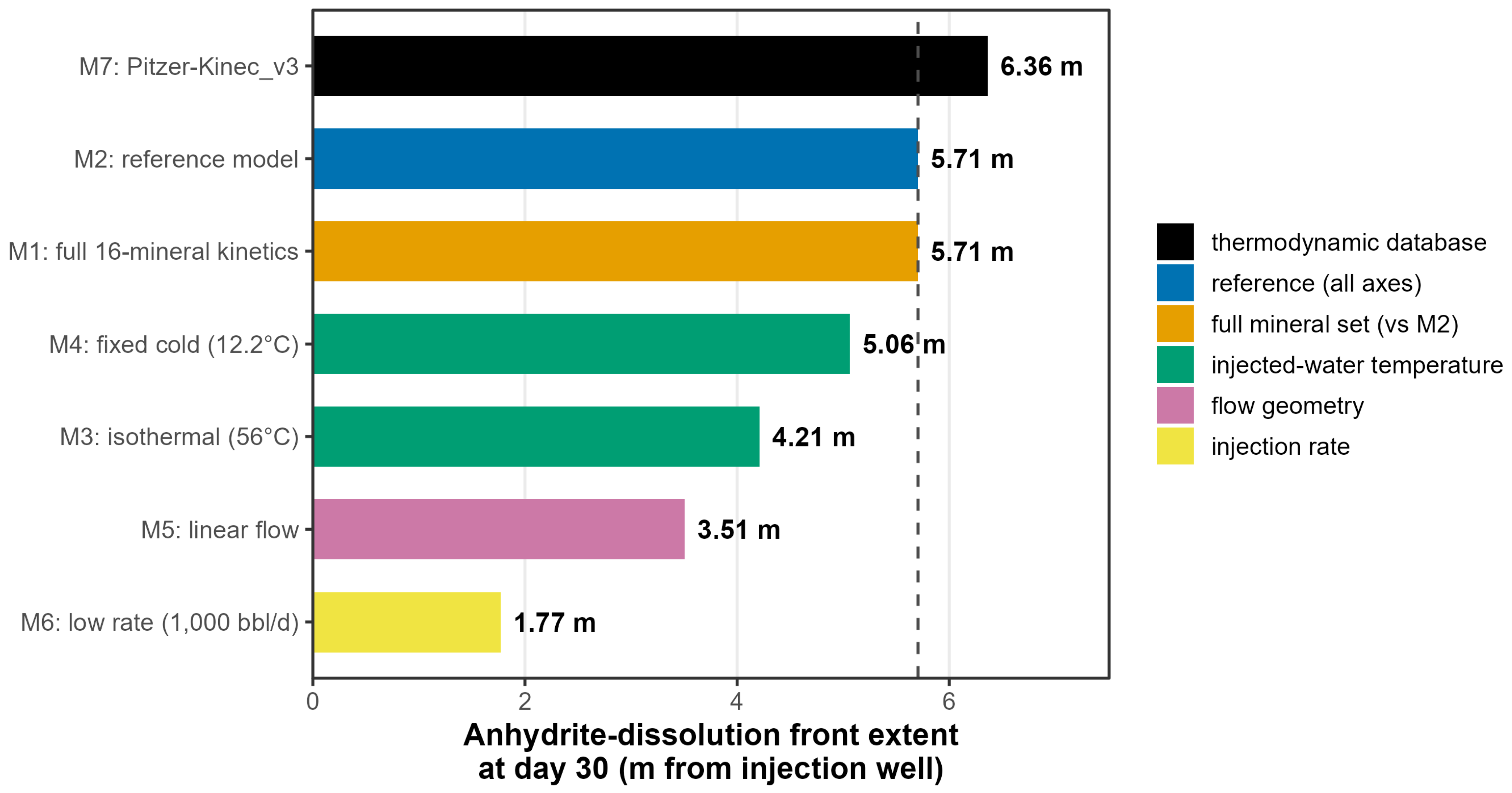
Figure 20.
Synthesis diagram revealing the position of the anhydrite dissolution (reaction) front at day 30, comparing radial and linear grids and 1000 and 10,000 bbl/d injection rates for the 12 key models (M2–M6 and M8–M14). The simulations are explained in Table 4. The front is defined as in Figure 19. (A) Radial simulations at 10,000 bbl/day injection with: Raley staged cooling (M2), no cooling effect (M3) and low-temperature seawater injection (M4). (B) Linear simulations at 10,000 bbl/day injection with: Raley staged cooling (M5), no cooling effect (M3) and low-temperature seawater injection (M9). (C) Radial simulations at 1,000 bbl/day injection with: Raley staged cooling (M6), no cooling effect (M10) and low-temperature seawater injection (M11). (D) Linear simulations at 1,000 bbl/day injection with: Raley staged cooling (M12), no cooling effect (M13) and low-temperature seawater injection (M14).
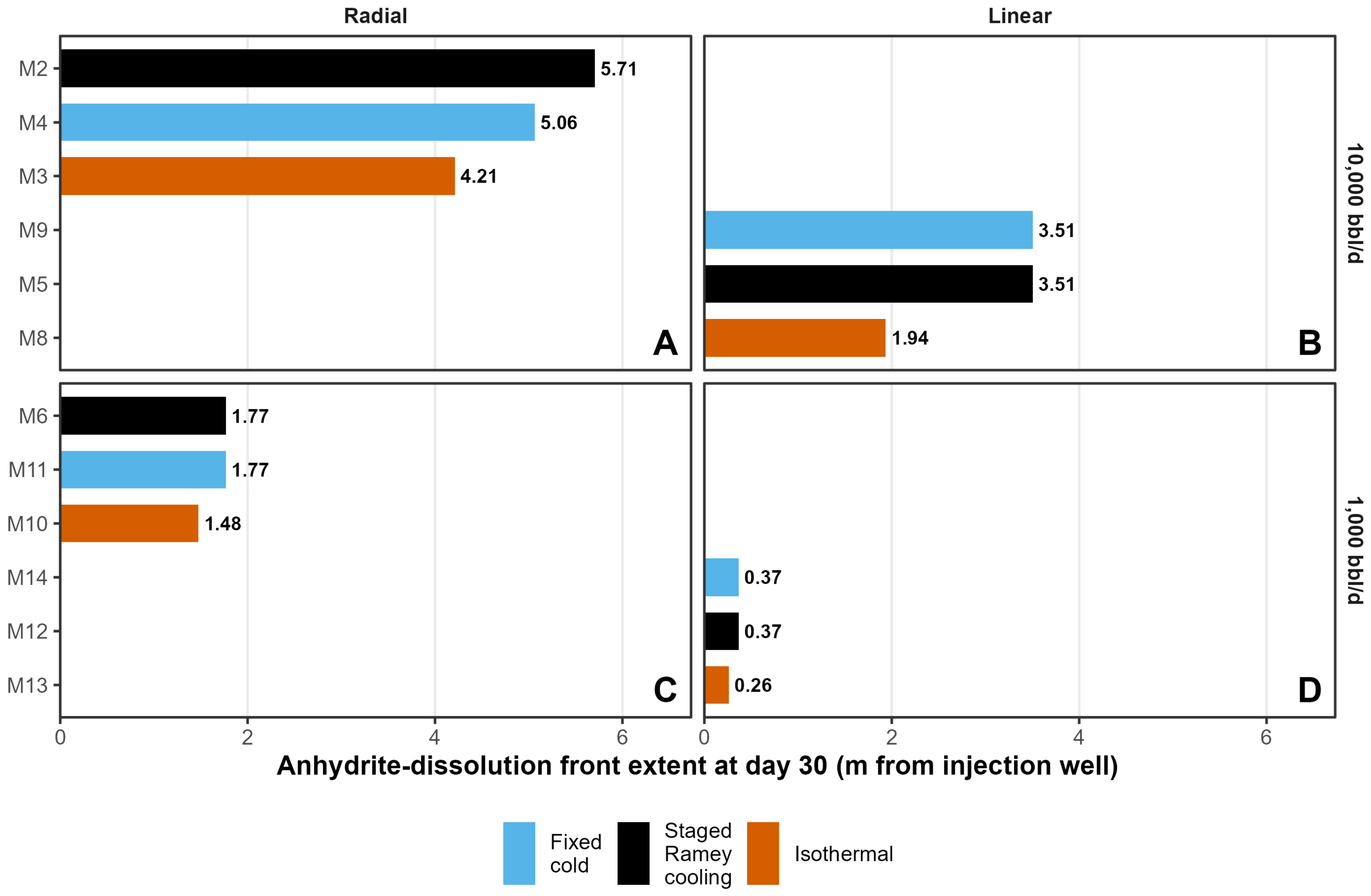
The factorial design corroborates the single-factor ranking, rate of seawater injection first, then flow geometry and then temperature regime (Figure 20). All three effects compress toward the linear, low-rate corner of the design, where grid resolution limits how far the front can be tracked, but this does not alter the ranking itself.
The temperature regime does not, however, act in the same direction on every part of the mineralogical result. Cooler water extends the anhydrite front because it can dissolve more anhydrite, whereas warmer water accelerates the kinetically limited growth of dolomite near the well (Section 3.8; Figure 16). Al-Behadili and Mackay [69] found that grid resolution (compare Figure 10) was the lowest-sensitivity factor among those that they tested for sulphate scaling in a seawater-flooded carbonate reservoir, well behind permeability heterogeneity. This is not in conflict with the models presented here. Grid resolution, in their study, meant refining the mesh within a single, already-chosen representation of the flow field, whereas the radial-versus-linear comparison made here is a change in the physical dimensionality of that representation itself, radially divergent flow around a well against one-dimensional flow through a column of constant cross-section, and Figure 9 traces the resulting difference directly to how each grid discretises distance rather than to any difference in reaction chemistry.
The safety of simplifying the mineral assemblage should also not be assumed to extend beyond the 30-day window examined here. The eight minerals frozen as inert in models M2 to M14, quartz, the feldspars, the clays, hematite and pyrite, are negligible only because their reaction kinetics are too slow to matter over 30 days (Figure 6); over the longer injection periods, or the extended shut-in periods, relevant to an operational CO2 store rather than a short pre-injection test, some of these phases could plausibly become significant, and the M1-against-M2 equivalence demonstrated here applies only to this timescale.
A related, but distinct, question is whether the initial mineral assemblage and the initial water chemistry are mutually consistent. A single-factor variant of the reference model, run with a 0.05 volume fraction of halite added to the mineral assemblage, shows the full 0.05 porosity increase implied by that volume fraction appearing everywhere in the grid within one day, regardless of distance from the well: this is not a transport-limited reaction front but an immediate response of the resident formation water itself, which is everywhere undersaturated with respect to halite (Table 3). It follows that halite cannot be carried in the kinetic mineral set at a volume fraction inconsistent with the modelled formation water’s own saturation state, whatever XRD data might suggest is locally present; this is a check on model consistency rather than a modelling-choice sensitivity of the kind ranked above. By contrast, a second single-factor variant, using the originally reported aqueous sulphate concentration of 385 mg/kgw [35] in place of the value elevated to 3903 mg/kgw for anhydrite pre-equilibration, makes a negligible difference to the porosity evolution (a 0.18% relative difference in the far-field cell, not growing with distance or time, and absent altogether in the near-well zone from day 2.5 onward), because the water controlling anhydrite dissolution throughout the swept zone is the injected seawater rather than the initial formation water. The aqueous sulphate concentration therefore behaves as a low-sensitivity input, alongside the kinetic mineral set and thermodynamic database choices identified above, whereas the halite content behaves as a hard constraint on model set-up rather than a tunable parameter.
Bringing the ranking together with these two caveats gives a practical recipe for building a screening reactive transport model of this kind. The injection rate, flow geometry and the injected-seawater temperature regime need to be represented correctly, because the predicted outcome depends materially on all three (Figure 19). A reduced mineral set and a simplified fixed-cold-temperature cooling schedule are acceptable simplifications for a 30-day model of seawater injection, and the extended Debye–Hückel activity model is acceptable for estimating the position of the front in seawater-dominated water, provided that the simulated duration remains short enough that the frozen minerals stay near-inert in practice, provided any mineral phase carried in the kinetic assemblage is first checked against the saturation state of the modelled formation water and provided that the thermodynamic database choice is revisited for any brine whose ionic strength lies far outside the calibration range of the simpler activity model, as Kinec_v3′s does for the Bunter Sandstone formation water used here. Wherever a calculation involves the formation brine itself, including the saturation indices, pre-equilibration of the formation water and scale prediction in the mixing zone, the Pitzer-Kinec_v3 approach of M7 (Figure 13) should be used. The laboratory hydration of anhydrite has required gypsum seeds or differential stress [49,73], and swelling of anhydritic rocks as they convert to gypsum in tunnels takes decades [74], both justifying gypsum growth being excluded from these models (see Section 2.4). However, gypsum growth could become relevant over longer injection periods. For an operational CO2 store, the replacement of anhydrite by gypsum in the cooled near-well zone, as predicted over decades of injection by [69], and its 61% increase in solid volume should be tested through reactive core-flood experiments.
5. Conclusions
- Under the conditions modelled, thirty days of seawater injection into the Bunter Sandstone is predicted to enhance rather than damage the near-well pore system: anhydrite dissolution raises porosity from 0.20 to about 0.226 in the swept zone, while near-well dolomite growth and far-field anhydrite precipitation are minor. Translated to permeability with a Kozeny–Carman relationship, this implies an illustrative 10–25% increase in aqueous injectivity index. Two independently published Bunter porosity–permeability relationships show that the porosity change is compatible with existing petrophysical trends, but neither validates the permeability of the reacted rock, which requires reactive core-flood experiments.
- The predicted dominance of anhydrite dissolution reflects the combination of the temperature, mineralogy and water composition, rather than a universal response to seawater injection. Although the adopted Bunter formation water is calcium-rich, the simulations predict net dissolution under the thermal and mixing conditions examined. Anhydrite saturation depends jointly on the temperature, seawater–formation-water mixing proportions and the resulting aqueous activities; published temperature or calcium thresholds should therefore not be treated as universal criteria for scale formation. Barite and celestite precipitation is negligible for the barium and strontium concentrations adopted here.
- Of the modelling choices tested, the injection rate, acting through the volume injected, has the largest effect on the reaction-front extent, with a 3.2-fold difference between 1000 and 10,000 bbl/d. Flow geometry ranks second, with the radial front extending approximately 63% further than the linear front, followed by injected-water temperature, with the isothermal front extending 26% less far than the staged-cooling reference case. Reducing the kinetic mineral set and halving or doubling the anhydrite and dolomite reactive surface areas have no detectable effect on the front position, although surface area modestly affects near-well dolomite growth. Using the merged Pitzer-Kinec_v3 database extends the front by approximately 12% relative to native Kinec_v3; this represents sensitivity to the combined thermodynamic formulation rather than to activity coefficients alone.
- A full 2 × 2 × 3 factorial completion of the injection-rate, flow-geometry and temperature-regime design (twelve models in total) shows that this ranking holds across every combination tested rather than a single comparison, with mean effects of 2.99 m, 1.67 m and 0.87 m, respectively, on the anhydrite front position, and reveals that the temperature regime affects the reservoir’s two reactive minerals in opposite directions: cooler injection extends the anhydrite-driven porosity front, while warmer isothermal injection increases near-well dolomite precipitation, roughly doubling it at the higher injection rate.
- These results give a practical basis for screening reactive transport models of this kind: injection rate, flow geometry and injected-water temperature must be represented correctly, whereas a reduced mineral set, a simplified cooling schedule and the assumed reactive surface area are acceptable simplifications for PHREEQC reactive transport modelling, as is the extended Debye–Hückel activity model for locating the front in seawater-dominated water, although the Pitzer model should be used for any calculation involving the formation brine, provided that the initial mineral assemblage remains consistent with the modelled formation water’s own saturation state.
- A sensitivity check found that including halite at a volume fraction of 0.05 in formation water undersaturated with respect to halite unsurprisingly caused it to dissolve everywhere in the grid within a day, an artefact of an incompatible initial condition rather than a transport-limited reaction, whereas the assumed aqueous sulphate concentration had negligible effect on the modelled porosity evolution.
- These conclusions hold for the 30-day, near-well window and formation water modelled here. Over the longer injection or shut-in periods relevant to an operational CO2 store, the reaction of minerals frozen as inert in this study could become significant, and the kinetics equivalence found here should not be extended without further testing. A subsequent lab-based study could usefully undertake reactive core-flood experiments using a Bunter Sandstone core and seawater at a bottom-hole temperature to confirm whether the geochemical porosity increase translates into a net increase in injectivity, given that cement dissolution could release fines or reduce grain support.
- No previously published study has combined kinetic reactive-transport modelling, an equal-pore-volume pseudo-radial PHREEQC grid and a staged wellbore-temperature boundary condition to assess seawater injectivity testing before CO2 storage. Applied here to the Bunter Sandstone Formation, the workflow also tests short-timescale mineral-assemblage simplification and compares the injection rate, flow representation and temperature regime in a factorial design. The individual methods have precedents, but their combination addresses this specific appraisal question in a new way. The workflow could be adapted to other storage aquifers; the minerals treated as inert, predicted reactions and implications for injectivity would need to be reassessed for each site, taking account of its mineralogy, brine composition, temperature and injection duration.
Funding
This research received no direct external funding.
Institutional Review Board Statement
Not applicable.
Informed Consent Statement
Not applicable.
Data Availability Statement
PHREEQC codes for all simulations plus the Excel spreadsheets used to convert raw XRD data into moles of mineral per kg of water and to derive mineral fractions and porosity following PHREEQC simulations are available at Zenodo (https://doi.org/10.5281/zenodo.23535140).
Acknowledgments
During the preparation of this manuscript, the author used AI tool Claude Opus 5 for the purpose of focused literature searches, forensic examination for errors in the R code used to plot the figures, proof-reading the revised manuscript and ensuring that all reviewers’ queries were addressed. Three reviewers are thanked for insightful comments that have led to a tighter set of results. The author has reviewed and edited the text and the diagrams and takes full responsibility for the content of this publication.
Conflicts of Interest
The author declares no conflicts of interest.
References
- IPCC. Global Warming of 1.5 °C. An IPCC Special Report on the Impacts of Global Warming of 1.5 °C Above Pre-Industrial Levels and Related Global Greenhouse Gas Emission pathways, in the Context of Strengthening the Global Response to the Threat of Climate Change, Sustainable Development, and Efforts to Eradicate Poverty; IPCC: Geneva, Switzerland, 2018. [Google Scholar]
- Haszeldine, R.S.; Flude, S.; Johnson, G.; Scott, V. Negative emissions technologies and carbon capture and storage to achieve the Paris Agreement commitments. Philos. Trans. R. Soc. A Math. Phys. Eng. Sci. 2018, 376, 20160447. [Google Scholar] [CrossRef] [Scilit] [PubMed]
- Worden, R.H. Carbon dioxide capture and storage (CCS) in saline aquifers versus depleted gas fields. Geosciences 2024, 14, 146. [Google Scholar] [CrossRef] [Scilit]
- Rigby, S.P.; Alsayaha, A. Storage sites for carbon dioxide in the North Sea and their particular characteristics. Energies 2024, 17, 211. [Google Scholar] [CrossRef] [Scilit]
- Karvounis, P.; Blunt, M.J. Assessment of CO2 geological storage capacity of saline aquifers under the North Sea. Int. J. Greenh. Gas. Control 2021, 111, 103463. [Google Scholar] [CrossRef] [Scilit]
- Alcalde, J.; Heinemann, N.; Mabon, L.; Worden, R.H.; de Coninck, H.; Robertson, H.; Maver, M.; Ghanbari, S.; Swennenhuis, F.; Mann, I.; et al. Developing full-chain industrial carbon capture and storage in a resource- and infrastructure-rich hydrocarbon province. J. Clean. Prod. 2019, 233, 963–971. [Google Scholar] [CrossRef] [Scilit]
- Rushton, J.C.; Hannis, S.; Pearce, J.; Williams, J.; Milodowski, A.E. Diagenetic evolution of the Bunter Sandstone Formation and its controls on reservoir quality: Implications for CO2 injectivity and storage. Geoenergy 2025, 3, geoenergy2024-023. [Google Scholar] [CrossRef] [Scilit]
- Allen, M.J.; Faulkner, D.R.; Worden, R.H.; Rice-Birchall, E.; Katirtsidis, N.; Utley, J.E.P. Geomechanical and petrographic assessment of a CO2 storage site: Application to the Acorn CO2 Storage Site, offshore United Kingdom. Int. J. Greenh. Gas. Control 2020, 94, 102923. [Google Scholar] [CrossRef] [Scilit]
- Turrell, W.R.; Berx, B.; Bresnan, E.; León, P.; Rouse, S.; Webster, L.; Walsham, P.; Wilson, J.; Wright, P. A review of national monitoring requirements to support offshore carbon capture and storage. Front. Mar. Sci. 2022, 9, 838309. [Google Scholar] [CrossRef] [Scilit]
- Baabbad, H.K.H.; Mugisha, J.; Shchipanov, A. Well testing before CO2 injection. In Proceedings of the Fifth EAGE Global Energy Transition Conference & Exhibition (GET 2024), Rotterdam, The Netherlands, 4–7 November 2024; pp. 1–5. [Google Scholar]
- Beretta, E.; Tiani, A.; Presti, G.L.; Verga, F. Injection tests as a reliable alternative to conventional well testing: A real field experience. SPE-100283-MS. In Proceedings of the SPE Europec/EAGE Annual Conference and Exhibition, Vienna, Austria, 12–15 June 2006. [Google Scholar]
- Cui, G.D.; Wang, Y.; Rui, Z.H.; Chen, B.L.; Ren, S.R.; Zhang, L. Assessing the combined influence of fluid-rock interactions on reservoir properties and injectivity during CO2 storage in saline aquifers. Energy 2018, 155, 281–296. [Google Scholar] [CrossRef] [Scilit]
- Gluyas, J.G.; Bagudu, U. The Endurance CO2 storage site, Blocks 42/25 and 43/21, UK North Sea. In United Kingdom Oil and Gas Fields: 50th Anniversary Commemorative Volume; Goffey, G., Gluyas, J.G., Eds.; Geological Society: London, UK, 2020; Volume 52, pp. 163–171. [Google Scholar]
- Okezie, C.C.; Bump, A.P. Calibrating large-scale injection: Using saltwater disposal experience to predict CCS performance on the Texas Gulf Coast. Int. J. Greenh. Gas. Control 2025, 147, 104485. [Google Scholar] [CrossRef] [Scilit]
- Liu, B.; Zhao, F.; Xu, J.; Qi, Y. Experimental investigation and numerical simulation of CO2-brine-rock interactions during CO2 sequestration in a deep saline aquifer. Sustainability 2019, 11, 317. [Google Scholar] [CrossRef] [Scilit]
- Fu, Y.J.; van Berk, W.; Schulz, H.M. Temporal and spatial development of scale formation: One-dimensional hydrogeochemical transport modeling. J. Pet. Sci. Eng. 2013, 112, 273–283. [Google Scholar] [CrossRef] [Scilit]
- Parkhurst, D.L.; Appelo, C.A.J. Description of input and examples for PHREEQC version 3—A computer program for speciation, batch-reaction, one dimensional transport, and inverse geochemical calculations. In U.S. Geological Survey Techniques and Methods; Book 6, Chapter A43; U.S. Geological Survey: Reston, VA, USA, 2013; 497p. [Google Scholar] [CrossRef] [Scilit]
- Oelkers, E.H.; Addassi, M. Kinec_v3: A computer database for the calculation of the dissolution rates of the major rock forming minerals. Chem. Geol. 2025, 695, 123041. [Google Scholar] [CrossRef] [Scilit]
- Ramey, H.J. Wellbore heat transmission. J. Pet. Technol. 1962, 14, 427–435. [Google Scholar] [CrossRef] [Scilit]
- Hasan, A.R.; Kabir, C.S. Aspects of wellbore heat transfer during two-phase flow. SPE Prod. Facil. 1994, 9, 211–216. [Google Scholar] [CrossRef] [Scilit]
- Hagoort, J. Ramey’s wellbore heat transmission revisited. SPE J. 2004, 9, 465–474. [Google Scholar] [CrossRef] [Scilit]
- Willhite, G.P. Over-all heat transfer coefficients in steam and hot water injection wells. J. Pet. Technol. 1967, 19, 607–615. [Google Scholar] [CrossRef] [Scilit]
- Raftogianni, A.; Vakalas, I.; Kiomourtzi, P.; Tsiantis, Y.; Apostolopoulos, G.; Pace, F.; Gaganis, V. Preliminary evaluation of geothermal potential in offshore depleted petroleum reservoirs: The Prinos-Kavala Basin, Northern Aegean, Greece. J. Mar. Sci. Eng. 2026, 14, 421. [Google Scholar] [CrossRef] [Scilit]
- Peaceman, D.W. Interpretation of well-block pressures in numerical reservoir simulation. Soc. Pet. Eng. J. 1978, 18, 183–194. [Google Scholar] [CrossRef] [Scilit]
- Gelhar, L.W.; Welty, C.; Rehfeldt, K.R. A critical review of data on field-scale dispersion in aquifers. Water Resour. Res. 1992, 28, 1955–1974. [Google Scholar] [CrossRef] [Scilit]
- Liu, P.; Yao, J.; Couples, G.D.; Ma, J.; Iliev, O. 3-D modelling and experimental comparison of reactive flow in carbonates under radial flow conditions. Sci. Rep. 2017, 7, 17711. [Google Scholar] [CrossRef] [Scilit] [PubMed]
- Appelo, C.; Van Loon, L.; Wersin, P. Multicomponent diffusion of a suite of tracers (HTO, Cl, Br, I, Na, Sr, Cs) in a single sample of Opalinus Clay. Geochim. Cosmochim. Acta 2010, 74, 1201–1219. [Google Scholar] [CrossRef] [Scilit]
- Kruisdijk, E.; van Breukelen, B. Reactive transport modelling of push-pull tests: A versatile approach to quantify aquifer reactivity. Appl. Geochem. 2021, 131, 104998. [Google Scholar] [CrossRef] [Scilit]
- Castillo, C.; Marty, N.C.M.; Hamm, V.; Kervévan, C.; Thiéry, D.; de Lary, L.; Manceau, J.-C. Reactive transport modelling of dissolved CO2 injection in a geothermal doublet. Application to the CO2-DISSOLVED concept. Energy Procedia 2017, 114, 4062–4074. [Google Scholar] [CrossRef] [Scilit]
- Wickham, H. Ggplot2: Elegant Graphics for Data Analysis; Springer: Cham, Switzerland, 2016; p. 226. [Google Scholar]
- Voigt, M.; Marieni, C.; Clark, D.E.; Gíslason, S.R.; Oelkers, E.H. Evaluation and refinement of thermodynamic databases for mineral carbonation. Energy Procedia 2018, 146, 81–91. [Google Scholar] [CrossRef] [Scilit]
- Helgeson, H.C. Thermodynamics of hydrothermal systems at elevated temperatures and pressures. Am. J. Sci. 1969, 267, 729–804. [Google Scholar] [CrossRef] [Scilit]
- Plummer, N.; Parkhurst, D.L.; Fleming, G.W.; Dunkle, S.A. A Computer Program Incorporating Pitzer’s Equations for Calculation of Geochemical Reactions in Brines: U.S. Geological Survey Water-Resources Investigations Report 88-4153; U.S. Geological Survey: Reston, VA, USA, 1988. [Google Scholar] [CrossRef] [Scilit]
- Pitzer, K.S. Thermodynamics of electrolytes. 1. Theoretical basis and general equations. J. Phys. Chem. 1973, 77, 268–277. [Google Scholar] [CrossRef] [Scilit]
- Capture Power Limited. K40: Subsurface Geoscience and Production Chemistry Reports. Technical: Storage Report Prepared for the UK Department of Energy and Climate Change (DECC) as Part of the White Rose Carbon Capture and Storage (CCS) Project; UK Government: London, UK, 2016; p. 300.
- Foote, N.; Hatter, S.J.; Gray, E.; Charlaftis, D. Reservoir characterization of the Triassic Bunter Sandstone in the 43/28-NEPBH1 borehole: Implications for CO2 storage in the neighbouring Endurance structure, Southern North Sea, UK. Geoenergy 2025, 3, geoenergy2025-012. [Google Scholar] [CrossRef] [Scilit]
- Warren, E.A.; Smalley, P.C. North Sea Formation Water Atlas; Geological Society: London, UK, 1994; Volume 15, p. 208. [Google Scholar]
- James, A.; Baines, S.; McCollough, S. D10: WP5A–Bunter Storage Development Plan; Pale Blue Dot Energy and Axis Well Technology: Loughborough, UK, 2016. [Google Scholar]
- Millero, F.J.; Feistel, R.; Wright, D.G.; McDougall, T.J. The composition of Standard Seawater and the definition of the Reference-Composition Salinity Scale. Deep Sea Res. Part I Oceanogr. Res. Pap. 2008, 55, 50–72. [Google Scholar] [CrossRef] [Scilit]
- Krauskopf, K.B. Introduction to Geochemistry, 2nd ed.; McGraw-Hill: Tokyo, Janpan, 1979. [Google Scholar]
- Beckingham, L.E.; Mitnick, E.H.; Steefel, C.I.; Zhang, S.; Voltolini, M.; Swift, A.M.; Yang, L.; Cole, D.R.; Sheets, J.M.; Ajo-Franklin, J.B.; et al. Evaluation of mineral reactive surface area estimates for prediction of reactivity of a multi-mineral sediment. Geochim. Cosmochim. Acta 2016, 188, 310–329. [Google Scholar] [CrossRef] [Scilit]
- Waldmann, S.; Busch, A.; van Ojik, K.; Gaupp, R. Importance of mineral surface areas in Rotliegend sandstones for modeling CO2-water-rock interactions. Chem. Geol. 2014, 378, 89–109. [Google Scholar] [CrossRef] [Scilit]
- AlNajdi, N.A.; Worden, R.H.; Utley, J.E.P. Compositional controls on the Lower Cretaceous Rodby Shale pore structure and surface area: A planned CCS top seal caprock for the Acorn storage site. Int. J. Greenh. Gas Control 2024, 137, 104219. [Google Scholar] [CrossRef] [Scilit]
- AlNajdi, N.; Worden, R.H.; Utley, J.E.P. The Palaeocene Lista Shale: A Planned Carbon Capture and Storage Top Seal for the East Mey CO2 Storage Site. Processes 2024, 12, 2773. [Google Scholar] [CrossRef] [Scilit]
- Xu, T.F.; Sonnenthal, E.; Spycher, N.; Pruess, K. TOUGHREACT–A simulation program for non-isothermal multiphase reactive geochemical transport in variably saturated geologic media: Applications to geothermal injectivity and CO2 geological sequestration. Comput. Geosci. 2006, 32, 145–165. [Google Scholar] [CrossRef] [Scilit]
- Gaus, I.; Azaroual, M.; Czernichowski-Lauriol, I. Reactive transport modelling of the impact of CO2 injection on the clayey cap rock at Sleipner (North Sea). Chem. Geol. 2005, 217, 319–337. [Google Scholar] [CrossRef] [Scilit]
- Palandri, J.L.; Kharaka, Y.K. U.S. Geological Survey Open File Report 2004-1068; A compilation of Rate Parameters of Water-Mineral Interaction for Application to Geochemical Modeling; USGS: Menlo Park, CA, USA, 2004.
- Blount, C.W.; Dickson, F.W. Gypsum-anhydrite equilibria in system CaSO4-H2O and CaSO4-NaCl-H2O. Am. Mineral. 1973, 58, 323–331. [Google Scholar]
- Hardie, L.A. The Gypsum-anhydrite equilibrium at one atmosphere pressure. Am. Mineral. 1967, 52, 171–200. [Google Scholar]
- Caselle, C.; Paschetto, A.; Costa, E.; Bonetto, S.; Giordano, E.; Mosca, P.; Ramon, A. Microstructural changes of anhydrite-gypsum samples during water immersion. Appl. Sci. 2026, 16, 2050. [Google Scholar] [CrossRef] [Scilit]
- Capture Power Limited. K41: Reservoir Engineering Field Report; White Rose CCS Project, Front-End Engineering Design Study, Report Prepared for the UK Department of Energy and Climate Change (DECC) as Part of the White Rose Carbon Capture and Storage (CCS) Project; UK Government: London, UK, 2016; p. 182.
- Harvie, C.E.; Moller, N.; Weare, J.H. The prediction of mineral solubilities in natural waters–the Na-K-Mg-Ca-H-Cl-SO4-OH-HCO3-CO3-CO2-H2O system at high ionic strength at 25 degrees C. Geochim. Cosmochim. Acta 1984, 48, 723–751. [Google Scholar] [CrossRef] [Scilit]
- Steefel, C.I.; Maher, K. Fluid-Rock Interaction: A Reactive Transport Approach. In Thermodynamics and Kinetics of Water-Rock Interaction; Oelkers, E.H., Schott, J., Eds.; Reviews in Mineralogy & Geochemistry; Mineralogical Society of America: Chantilly, VA, USA, 2009; Volume 70, pp. 485–532. [Google Scholar] [CrossRef] [Scilit]
- Rushton, J.C.; Hannis, S.; Milodowski, A.E. Petrography and Diagenesis of the Bunter Sandstone Formation in the UK Southern North Sea; British Geological Survey Open Report: Keyworth, UK, 2023; p. 59. [Google Scholar]
- Oelkers, E.H.; Addassi, M. A comprehensive and consistent mineral dissolution rate database: Part III: Non-silicate minerals including carbonate, sulfate, phosphate, halide, and oxy-hydroxide minerals. Chem. Geol. 2025, 673, 122528. [Google Scholar] [CrossRef] [Scilit]
- Tiab, D.; Donaldson, E.C. Petrophysics, 4th ed.; Elsevier: Amsterdam, The Netherlands, 2015; p. 894. [Google Scholar]
- Capture Power Limited. K43: Field Development Report–Technical: Storage Report Prepared for the UK Department of Energy and Climate Change (DECC) as Part of the White Rose Carbon Capture and Storage (CCS) Project; UK Government: London, UK, 2016.
- Gibson-Poole, C.M.; Tarasewicz, J.; Gray, E.; Hitchen, K.; Bouffin, N.; Taplin, M.; Gillespie, A.; Buchanan, S.K. Endurance saline aquifer CO2 store–from appraisal to development and beyond. In Powering the Energy Transition Through Subsurface Collaboration: Proceedings of the 1st Energy Geoscience Conference; Gill, C., Goffey, G., Underhill, J.R., Eds.; Geological Society: London, UK, 2025. [Google Scholar] [CrossRef] [Scilit]
- Bela, R.V.; Pesco, S.; Barreto, A. Determining skin zone properties from injectivity tests in single- and multilayer reservoirs. J. Pet. Explor. Prod. Technol. 2020, 10, 1459–1471. [Google Scholar] [CrossRef] [Scilit]
- Hawkins, M.F. A note on the skin effect. Trans. Am. Inst. Min. Metall. Eng. 1956, 207, 356–357. [Google Scholar] [CrossRef] [Scilit]
- Khilar, K.C.; Fogler, H.S. The existence of a critical salt concentration for particle release. J. Colloid Interface Sci. 1984, 101, 214–224. [Google Scholar] [CrossRef] [Scilit]
- Houston, S.J.; Yardley, B.W.D.; Smalley, P.C.; Collins, I. Rapid fluid-rock interaction in oilfield reservoirs. Geology 2007, 35, 1143–1146. [Google Scholar] [CrossRef] [Scilit]
- McCartney, R.A. Conditions Under Which Anhydrite Precipitation Can Occur in Oil Reservoirs as a Result of Seawater Injection. Available online: http://oilfieldwaterservices.co.uk/wp-content/uploads/2014/05/McCartney-2008.pdf (accessed on 21 September 2026).
- Al-Behadili, A.M.; Mackay, E.J. Impact of geochemical reactivity on desulphation requirements in a sandstone reservoir containing carbonate and sulphate minerals. Front. Chem. 2025, 13, 1540250. [Google Scholar] [CrossRef] [Scilit] [PubMed]
- Hajiabadi, S.H.; Bedrikovetsky, P.; Borazjani, S.; Mahani, H. Well injectivity during CO2 geosequestration: A review of hydro-physical, chemical, and geomechanical effects. Energy Fuels 2021, 35, 9240–9267. [Google Scholar] [CrossRef] [Scilit]
- Osborne, C.G.; Ravenscroft, P.D.; McCracken, I.R. Predicted water chemistry trends in North Sea formation brines. Mar. Pet. Geol. 1994, 11, 20–23. [Google Scholar] [CrossRef] [Scilit]
- Yuan, M.D.; Todd, A.C.; Sorbie, K.S. Sulfate scale precipitation arising from seawater injection—A prediction study. Mar. Pet. Geol. 1994, 11, 24–30. [Google Scholar] [CrossRef] [Scilit]
- Kermani, H.M.; Bonto, M.; Nick, H.M. Chemical solutions for restoring scaling-induced injectivity impairment in offshore produced water re-injection. Sci. Total Environ. 2023, 903, 166597. [Google Scholar] [CrossRef] [Scilit] [PubMed]
- Al-Behadili, A.M.; Mackay, E.J. Effects of permeability, grid resolution, and carbonate reactions on CO2 distribution and sulphate scaling in seawater-flooded carbonates. Sci. Rep. 2025, 15, 29287. [Google Scholar] [CrossRef] [Scilit] [PubMed]
- Tranter, M.; De Lucia, M.; Wolfgramm, M.; Kühn, M. Barite scale formation and injectivity loss models for geothermal systems. Water 2020, 12, 3078. [Google Scholar] [CrossRef] [Scilit]
- Appelo, C.A.J.; Postma, D. Geochemistry, Groundwater and Pollution, 2nd ed.; A. A. Balkema Publishers: Leiden, The Netherlands, 2005. [Google Scholar]
- Lichtner, P.C. The quasi-stationary state approximation to coupled mass-transport and fluid-rock interaction in a porous medium. Geochim. Cosmochim. Acta 1988, 52, 143–165. [Google Scholar] [CrossRef] [Scilit]
- Heeb, J.; Healy, D.; Timms, N.E.; Gomez-Rivas, E. Rapid hydration and weakening of anhydrite under stress: Implications for natural hydration in the Earth’s crust and mantle. Solid Earth 2023, 14, 985–1003. [Google Scholar] [CrossRef] [Scilit]
- Serafeimidis, K.; Anagnostou, G. On the time-development of sulphate hydration in anhydritic swelling rocks. Rock Mech. Rock Eng. 2013, 46, 619–634. [Google Scholar] [CrossRef] [Scilit]
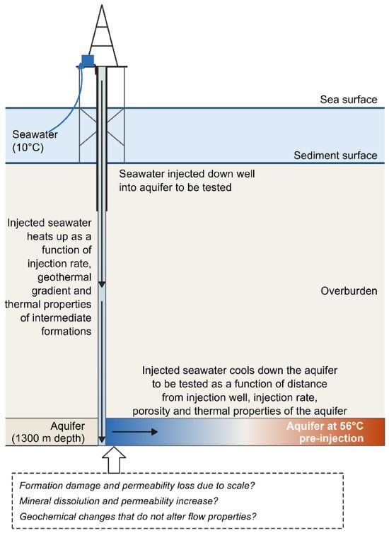
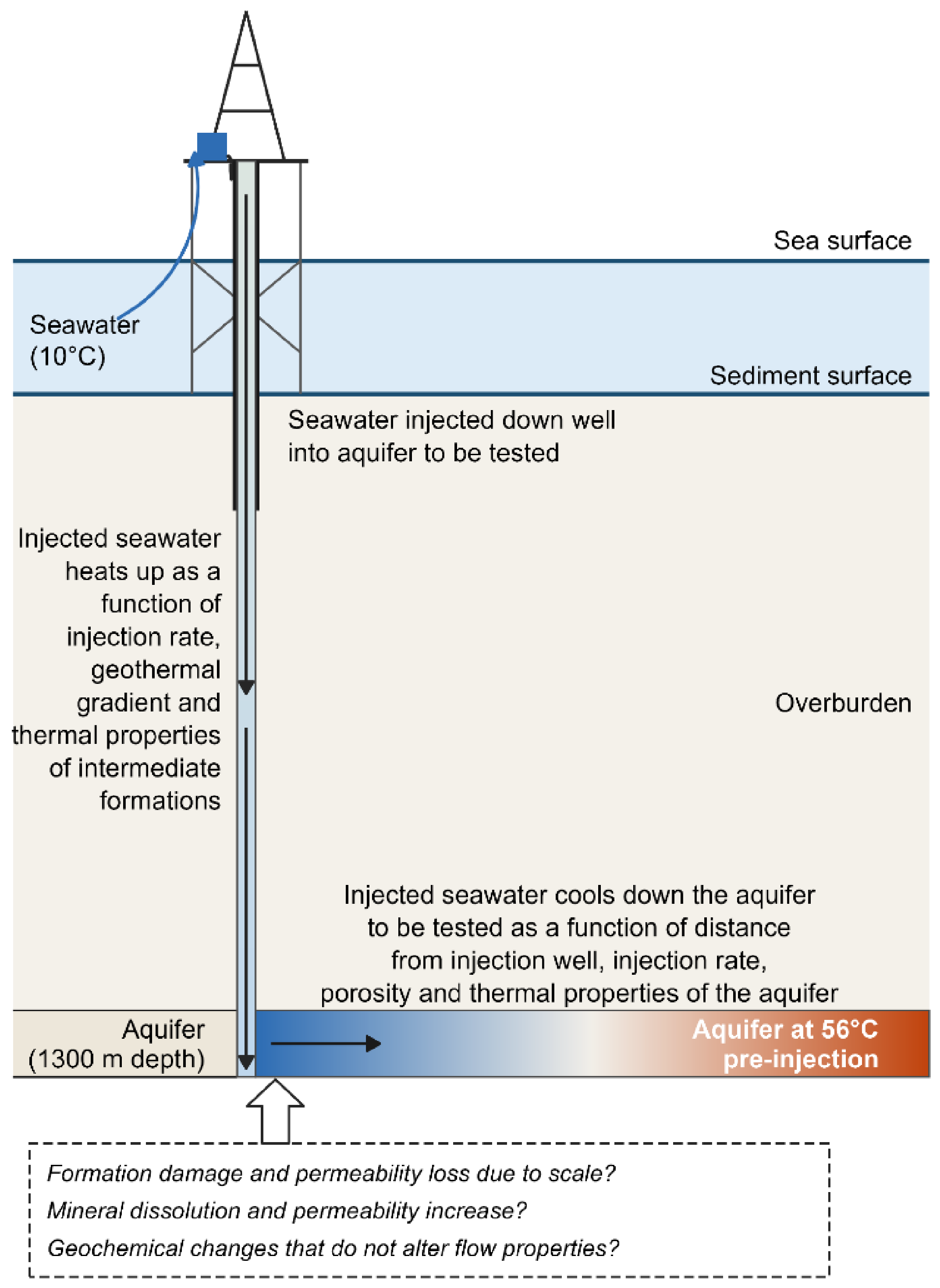
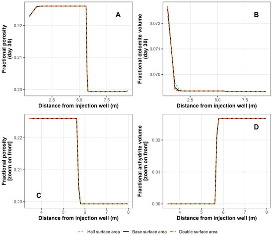
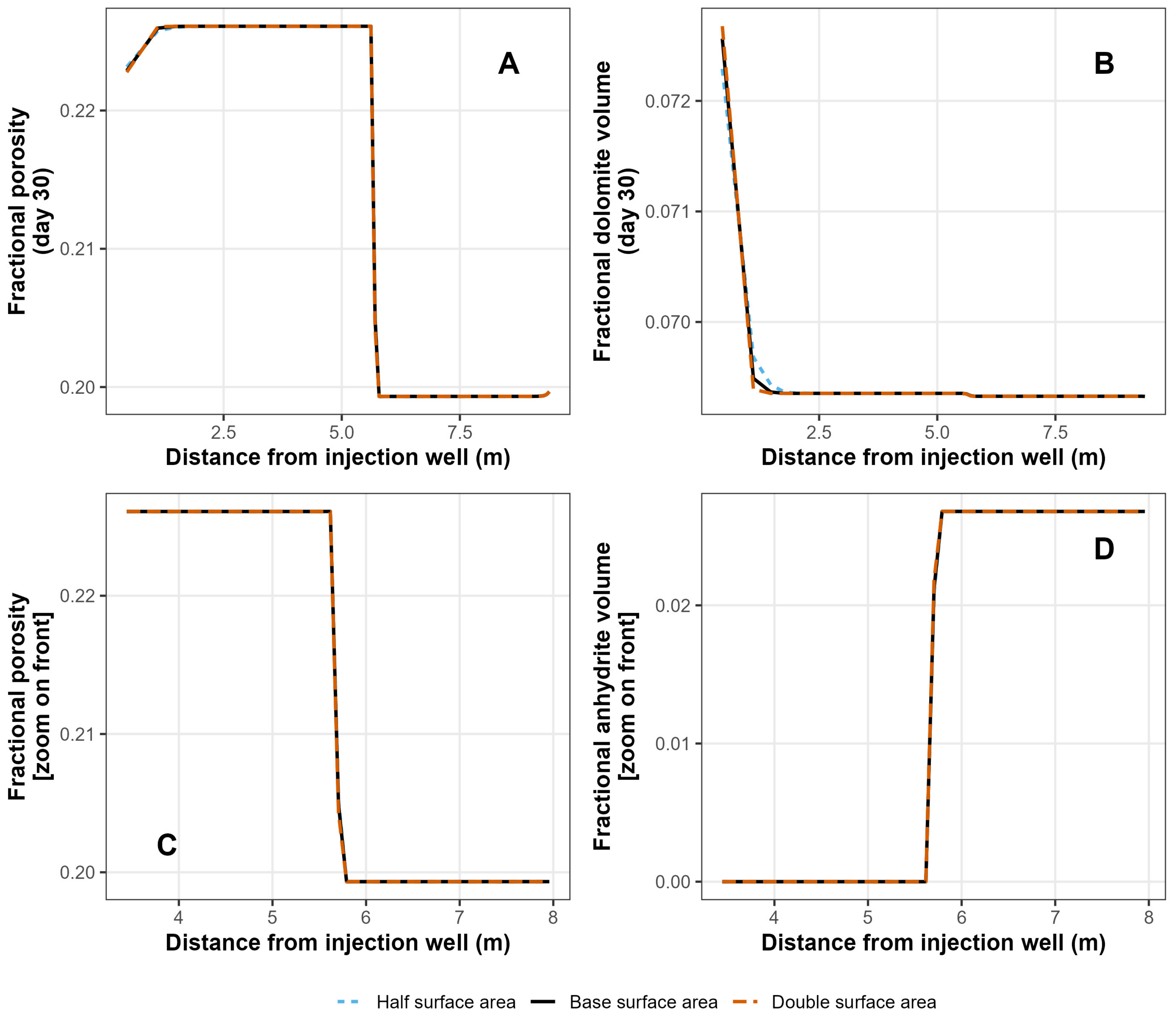

Disclaimer/Publisher’s Note: The statements, opinions and data contained in all publications are solely those of the individual author(s) and contributor(s) and not of MDPI and/or the editor(s). MDPI and/or the editor(s) disclaim responsibility for any injury to people or property resulting from any ideas, methods, instructions or products referred to in the content. |
© 2026 by the author. Licensee MDPI, Basel, Switzerland. This article is an open access article distributed under the terms and conditions of the Creative Commons Attribution (CC BY) license.