


Abstract
With the rapid development of artificial intelligence technologies and the increasing energy demand of data centers, energy systems need to be operated with increasing reliability and flexibility. To address operational risks caused by renewable energy fluctuations and random equipment failures, this study takes a distributed integrated energy system for a data center as the research object and proposes an optimal scheduling strategy that coordinates dynamic reliability and flexibility. First, a dynamic reliability assessment model is established using a sequential Monte Carlo simulation based on a two-state Markov model, and the system’s reliability is quantitatively evaluated using the loss of load probability (LOLP) and expected energy not supplied (EENS). Second, equipment-level and system-level flexibility margin models are developed, and a dynamic reliability baseline constraint is introduced to integrate reliability requirements and regulation capability into a unified optimal scheduling framework. Finally, a simulation case based on the characteristics of a data center in Lingang, Shanghai, is used to evaluate the proposed method under typical seasonal operating conditions. The results show that the proposed strategy can effectively improve energy supply reliability and operational flexibility. Under typical summer conditions, the EENS of the cooling system is reduced by 82.3% compared with the conventional strategy, while the total system operating cost is reduced by 10.93–15.16% under different seasonal conditions. The proposed framework provides an effective approach for the reliability–flexibility-coordinated operation of data center integrated energy systems.
1. Introduction
The ongoing low-carbon energy transition and rapid advances in artificial intelligence have driven a marked increase in both the scale and energy consumption of data centers, which serve as critical infrastructure for the digital economy. The sustained high-intensity operation of server clusters and cooling equipment imposes stringent requirements on the continuity and reliability of the energy supply. Traditional data centers, however, rely predominantly on external power grids and centralized supply modes, resulting in low energy efficiency and limited regulation flexibility. To address these deficiencies, the integration of distributed energy resources; energy storage; and combined cooling, heating, and power (CCHP) systems into a data center integrated energy system (IES) has become a promising direction. By coordinating electricity, natural gas, and thermal energy, the IES can fully exploit multi-energy complementarity, thereby improving both operational flexibility and economic performance [1,2,3,4,5].
With the increasing penetration of renewable energy, the operation of data center integrated energy systems faces growing uncertainty from renewable generation fluctuations, load variations, and stochastic equipment failures. These uncertainties not only affect the economic operation of the system but also challenge the continuous and reliable energy supply required by data centers. Compared with conventional energy systems, a data center IES involves strong coupling among multiple energy flows and complex interactions among energy conversion equipment, storage devices, and flexible loads. Consequently, ensuring reliable operation while maintaining sufficient regulation capability under uncertain conditions has become a key challenge for sustainable data center energy management.
In recent years, data center operators have gradually adopted low-carbon strategies such as renewable electricity procurement and green electricity certificates (green energy certificates) to reduce the carbon footprint associated with electricity consumption. These approaches mainly reduce emissions from the energy supply side by improving the carbon characteristics of the consumed electricity. However, operational scheduling strategies determine how available energy resources are dynamically utilized under different operating conditions and directly influence the coordination between renewable generation, energy storage, and multi-energy conversion devices. Therefore, flexibility-oriented scheduling provides an important operational pathway for supporting sustainable energy utilization. Nevertheless, due to the lack of mature dynamic carbon emission factor models that can accurately describe real-time variations in electricity carbon intensity, the quantitative contribution of operational flexibility to carbon reduction remains difficult to evaluate. Thus, sustainable data center operation requires not only low-carbon energy supply structures but also reliable and flexible operational management strategies.
1.1. Reliability Quantification and Characterization of Integrated Energy Systems
Compared with that on traditional power systems, reliability research on integrated energy systems (IESs) remains nascent. Existing reliability theories are primarily tailored to single-energy networks, whereas an IES is characterized by multi-energy coupling and heterogeneous coordination. Hence, establishing a unified evaluation framework that accommodates both overall system reliability and the distinct characteristics of electricity, heat, and natural gas remains a considerable challenge.
Extensive research on IES reliability assessment has been conducted in recent years. Reference [6] combines analytical and simulation methods to evaluate the reliability of wind power systems with energy storage. Reference [7] develops a data-driven reliability assessment model based on machine learning. Reference [8] improves the computational efficiency of reliability evaluation via an enhanced state-enumeration approach. References [9,10] establish reliability analysis models for electricity–gas coupled networks and for IESs under uncertainty scenarios, respectively. References [11,12] further integrate intelligent-agent algorithms with Markov multi-state simulation to achieve reliability measurement and assessment for IESs.
Regarding reliability-constrained optimal scheduling, Reference [13] combines dynamic optimal energy flow with Monte Carlo simulation to realize emergency dispatch under fault scenarios. Reference [14] constructs a multi-objective optimization model that balances economic performance, low-carbon performance, and flexibility. Reference [15] adopts hybrid game-theoretic optimal scheduling and employs a state-similarity method to ensure reliable and economic IES operation. Reference [16] develops a thermal-storage-based rolling-horizon scheduling framework for regional integrated energy systems and incorporates Markov simulation to evaluate reliability and resilience.
In summary, existing studies have made significant progress in IES reliability assessment and reliability-constrained scheduling. However, most of them emphasize either reliability evaluation or economic optimization, with insufficient in-depth characterization of the synergy between dynamic reliability and system flexibility. Moreover, the impacts of equipment ramping constraints, fault evolution processes, and multi-energy-flow dynamic regulation capabilities on operational reliability have not been fully considered. Therefore, it is necessary to develop an optimal scheduling approach that jointly accommodates dynamic reliability and flexibility requirements, to enhance the security and economic performance of IESs under complex operating conditions.
1.2. Quantification and Characterization of Flexibility Margins for IES in Demand Response
Flexibility is generally defined as the ability of a system to cope with supply–demand fluctuations and uncertain disturbances while maintaining dynamic equilibrium operation. The International Energy Agency (IEA) defines flexibility as the capability of an energy system to adjust supply and demand in response to variability and uncertainty [17]. Flexibility therefore represents the ability of the system to coordinate available resources and maintain reliable operation under changing operating conditions. Although a unified definition has not yet been established, the essence of flexibility consistently reflects the system’s capacity to absorb disturbances and adapt to changes across different timescales [18]. For integrated energy systems (IESs), flexibility derives not only from the inherent regulation potential of multiple energy resources—including electricity, heat, cooling, and natural gas—but also from the synergistic complementarity among different energy subsystems under multi-energy coupling conditions [19,20,21,22].
The flexibility margin is a critical indicator for characterizing system regulation capability and adjustable capacity, and serves as the foundation for system planning and optimal scheduling. However, the evaluation framework and quantification methods for IES flexibility are still in the developmental stage [23]. In recent years, extensive research has been conducted on flexibility modeling and assessment. Reference [24] constructs a flexibility evaluation framework for an electricity–heat–water coupled system. Reference [25] exploits the regulation potential of heat loads to achieve peak load shaving in distribution networks. Reference [26] analyzes the economic value of flexible resources participating in electricity markets. Reference [27] establishes a multi-dimensional flexibility evaluation index system. Reference [28] investigates the impact of flexibility pricing mechanisms on IES operational benefits. Reference [29] further proposes a flexibility quantification method that accounts for spatiotemporal coupling characteristics.
In summary, existing studies predominantly focus on single power systems or specific flexibility resources, with insufficient characterization of comprehensive flexibility under the coupling of multiple energy carriers such as electricity, heat, and cooling. Moreover, the coupling relationship between system flexibility and operational reliability has not been thoroughly investigated, making it difficult to reflect the multi-energy synergistic regulation capability under complex operating environments. Therefore, it is necessary to develop a flexibility evaluation and optimal scheduling approach for IES that jointly accommodates dynamic reliability and flexibility requirements, thereby supporting secure and economic operation under the context of high-penetration renewable energy integration [30,31].
1.3. Research Content and Contributions
To address the aforementioned issues, this study takes a distributed integrated energy system of a data center as the research object and proposes an optimal scheduling strategy that coordinates dynamic reliability and flexibility. First, the equipment operation models and the dynamic reliability assessment model are established, with the sequential Monte Carlo simulation based on a two-state Markov model method employed to characterize the dynamic state transition processes of the equipment. Second, the concept of a dynamic reliability baseline is introduced to quantify the required reserve capacity under high-confidence fault scenarios based on a predefined reliability confidence level. On this basis, a flexibility margin model is further developed above the baseline, and the dynamic reliability, flexibility, and system economic operation objectives are uniformly incorporated into the optimization framework, thereby achieving the coordinated optimization of energy supply reliability and operational economy.
The main contributions of this study are as follows:
- (1)
- A dynamic reliability model for the integrated energy system is established that accounts for the dynamic state transition processes of equipment, enabling the dynamic quantification of system operational risk. Furthermore, a dynamic reliability baseline model is proposed to characterize the reliability reserve boundary of the system under high-confidence fault scenarios based on scenario-based quantile estimation.
- (2)
- A flexibility margin model based on reliability constraints is constructed, achieving the coordinated optimization of reliability and operational economy for the high-efficiency data center chiller plant system.
2. Methodology
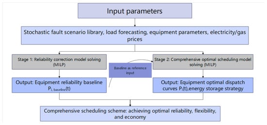
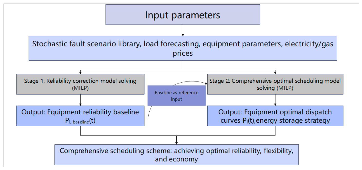
To address the challenge of coordinating reliability and flexibility in data center integrated energy systems under the influence of renewable energy fluctuations and stochastic equipment failures, this study constructs an optimal scheduling model that incorporates dynamic reliability. First, the key equipment models and the energy balance model of the system are established. Then, the system dynamic reliability is evaluated based on the sequential Monte Carlo simulation based on a two-state Markov model method, and a dynamic reliability baseline is constructed. On this basis, a flexibility margin model above the baseline is developed to achieve a unified characterization of both the reliability requirements and regulation capability demands of the system. Finally, an optimal scheduling model is formulated with the objective of minimizing the total operating cost, thereby achieving the coordinated optimization of system reliability, flexibility, and economy. The overall solution procedure of the proposed reliability–flexibility coordinated scheduling framework is illustrated in Figure 1.
Figure 1.
Flowchart of the solution process for the optimal scheduling model of the integrated energy system considering dynamic reliability.
2.1. Energy Supply Equipment Modeling
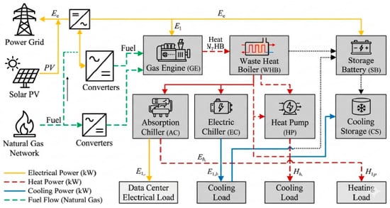
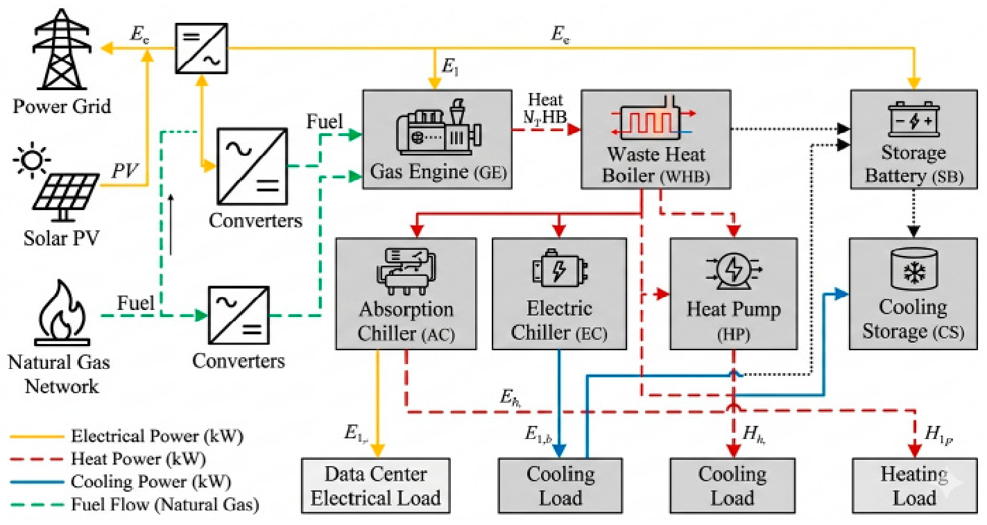
Against the backdrop of growing renewable energy integration and the typical energy consumption characteristics of distributed systems, this study selects a data center as the research platform and constructs an IES physical architecture, as shown in Figure 2. On the electrical supply side of this architecture, the data center is supplied by the public power grid, with a gas engine (GE) undertaking the base power generation task, supplemented by a photovoltaic (PV) array deployed outside the equipment room. The electricity from these sources is consolidated into an uninterruptible power supply (UPS), which then delivers stable power to the entire campus. On the cooling–heating interaction side, an electric chiller (EC) and an absorption chiller (AC) constitute the primary sources of the cooling load. Meanwhile, the waste heat generated during the cooling process is directed to a heat pump (HP) for cascaded utilization, partially filling the cooling and heating gaps. In addition, the waste heat exhausted by the GE is captured by a waste heat boiler (WHB), which is primarily used to drive the AC units for cooling, with the remaining heat directly utilized for heating. To optimize operating costs and reduce the peak supply pressure, the platform also integrates a storage battery (SB) and a cold storage device (CS), enabling an economic regulation strategy of “charging at off-peak periods and discharging at peak periods”, while also serving as an emergency backup power source under system outage conditions.
Figure 2.
Topology of the integrated energy system for the data center.
2.2. System Energy Balance Constraints
As shown in Figure 2, the supply–demand balance constraints for the electricity, heat, and cooling of the integrated energy system are formulated as follows:
- (1)
- Electric power balance:
The electrical output of the gas engine is related to its natural gas consumption through
where Fg,t is the natural gas consumption rate, Hg is the calorific value of natural gas, and ηGE is the electrical efficiency of the gas engine.
In Equation (2), the gas engine output is calculated based on fuel consumption and electrical conversion efficiency. Therefore, the parameter represents the fuel-based electrical efficiency rather than a heat-to-electricity ratio.
The dynamic energy state of the battery is described as
where Eb,t is the stored electrical energy, is the self-discharge rate, and and are the charging and discharging efficiencies, respectively.
The allowable battery energy range is constrained by
To avoid simultaneous charging and discharging of the battery, binary operation variables are introduced. The charging and discharging states of the battery are constrained as follows:
where uch,t and udis,t are binary variables representing the charging and discharging states of the battery, respectively. These constraints ensure that the battery cannot perform charging and discharging operations simultaneously.
where uch,t and udis,t are binary variables indicating the charging and discharging states of the battery, respectively. The initial and terminal energy states of the battery are defined as
where SOCinit represents the initial state of charge. The terminal SOC constraint is introduced to maintain daily operation continuity.
- (2)
- Thermal balance:
The waste heat recovered from the gas engine is expressed as
where VNG,t is the natural gas consumption rate of the gas engine (m3/h), HNG is the lower heating value of natural gas (kWh/m3), and is the waste heat recovery coefficient of the gas engine. Accordingly, the recovered waste heat is determined by the fuel energy input rather than by directly multiplying the electrical output by the waste heat recovery coefficient.
The heat output of the waste heat boiler is
where is the recoverable waste heat from the gas engine calculated using Equation (9), and ηWHB is the heat recovery efficiency of the waste heat boiler.
The cooling output of the absorption chiller is related to its thermal input by
where COPAC is the coefficient of the performance of the absorption chiller.
- (3)
- Cooling balance:
For the electric chiller:
where COPEC is the coefficient of the performance of the electric chiller.
For the heat pump in cooling mode:
where is the cooling coefficient of the performance.
The dynamic state of the cold storage unit is expressed as
where Ec,t is the stored cooling energy, λc is the cooling loss rate, and and are the charging and discharging efficiencies of the cold storage unit, respectively.
The energy state of the cold storage unit is constrained by
and simultaneous charging and discharging are prevented by
The initial and terminal energy states of the cold storage unit are defined as
where Ecs,init represents the initial stored cooling energy. The terminal condition is applied to maintain energy balance consistency over the scheduling horizon.
In addition, the cold storage loss coefficient is defined based on the 15 min dispatch interval.
2.3. Dynamic Reliability Assessment
Under the influence of uncertain factors such as renewable energy fluctuations, stochastic load variations, and equipment failures, satisfying energy balance conditions alone is insufficient to guarantee adequate energy supply reliability and dynamic regulation capability. Therefore, based on the established energy balance models for the power system and cooling system, a sequential Monte Carlo simulation method based on a two-state Markov model is adopted to dynamically characterize equipment operating states. The system reliability is quantified using the loss of load probability (LOLP) and expected energy not supplied (EENS).
A sequential Monte Carlo simulation based on two-state Markov models is employed to generate stochastic equipment operating states. A 15 min time step is adopted to maintain consistency with the dispatch resolution. The simulation covers a two-year chronological horizon, corresponding to 70,080 time intervals. All components are initialized in the normal operating state, and their subsequent transitions are determined by the specified failure and repair probabilities. A fixed random seed of 2026 is used to ensure reproducibility.
For the scenario-based dispatch calculations, 10,000 equipment-state configurations are selected from the generated chronological sequence. These configurations are evaluated against the load conditions of each of the 96 dispatch intervals of a representative day. Thus, the sample size of 10,000 refers to equipment-state configurations rather than independent two-year trajectories. The selected sample size represents a computational compromise between scenario coverage and optimization burden.
During fault scenarios, the available capacity of failed equipment is modified according to its operating state. For equipment i, the output constraint is adjusted as
where zi,t represents the equipment operating state obtained from the sequential Monte Carlo simulation. When zi,t = 0, the corresponding equipment output is unavailable. In this case, both the lower and upper output bounds of the failed equipment are set to zero, forcing its output to zero. For storage devices, failure states are assumed to result in unavailable charging/discharging capability, while stored energy is maintained until recovery.
To further quantify the sampling uncertainty of the Monte Carlo reliability estimates, a nonparametric bootstrap procedure is adopted based on the 10,000 sampled equipment-state configurations. In each bootstrap replication, 10,000 configurations are randomly drawn with replacement from the original sample, and the reliability indices, including LOLP and EENS, are recalculated using the same assessment procedure. The 95% confidence intervals are determined by the 2.5th and 97.5th percentiles of the bootstrap estimates. The resampling unit is the equipment-state configuration rather than the individual 15 min dispatch interval. This procedure quantifies the sampling variability across the selected configurations. The random seed is fixed to ensure reproducibility.
The following assumptions are adopted in the reliability simulation:
- (1)
- The failure and repair processes of individual components are modeled using independent two-state Markov models.
- (2)
- Common-cause failures among multiple components are not explicitly considered.
- (3)
- The external power grid is assumed to have a high availability level and is not modeled as a stochastic failure component in this study.
- (4)
- The UPS system is considered as a backup protection device and is not explicitly included in the stochastic failure model.
2.3.1. Dynamic Reliability Model of Energy Conversion Equipment
The key equipment in the integrated energy system is subject to stochastic failures and repairs during operation, and its operating states evolve dynamically over time. To accurately characterize the equipment state transition process, this study adopts a dynamic reliability model based on Markov chains to model the equipment operating states. The equipment is represented by a two-state model, namely the normal operating state (State 0) and the faulty state (State 1), with the transition between the two states governed by the failure rate λ and the repair rate μ, respectively.
Because the failure outage of an independent equipment is a stochastic process {X(t), t ∈ T}} that evolves over time, according to Markov chain theory, within an infinitesimal time step Δt, the state transition probability of the i-th equipment can be approximated as follows:
where is the probability that the i-th equipment transits from State 0 to State 1,
is the probability that the i-th equipment transits from State 1 to State 0, is the probability that the i-th equipment remains in State 0, and is the probability that the i equipment remains in State 1.
In this model, the state transition process is assumed to involve no secondary transitions. At the probability measure level, this simplification allows the transition matrix elements to become numerically approximately equivalent to the inherent failure probabilities of the equipment.
Define , j ∈ E, as the probability that the i-th equipment is in state j. Then it can be derived that
By substituting different state parameters j into the above equation, the probability distributions of the component under steady-state operation and forced outage conditions can be derived, respectively:
Through derivation and solving, the dynamic probability distribution of equipment i at time t can be explicitly expressed as follows:
2.3.2. Reliability Assessment Indices
Considering the similarity in energy supply mechanisms among the electricity, heat, and cooling multi-energy networks within the integrated energy system, this study adopts loss of load probability (LOLP) and expected energy not supplied (EENS) as system reliability evaluation indices and extends them to multi-energy scenarios to quantify the system energy supply reliability level.
- (1)
- Loss of Load Probability
For conventional power systems, the loss of load probability (LOLP) represents the probability that the available energy supply capacity is insufficient to satisfy the load demand. In the Monte Carlo simulation framework, LOLP is calculated based on the occurrence frequency of insufficient supply states among all sampled operating scenarios.
where N is the total number of random sampling iterations, Ns is the number of Monte Carlo sampled trajectories and T = 96 is the number of 15 min dispatch intervals in each representative day. FLOLP(XI) is the interval-level test function that equals 1 when the available supply is insufficient to meet the load demand and 0 otherwise. Thus, Equation (11) averages the shortage indicators over all 96 intervals of each sampled trajectory and across all Ns trajectories.
Accordingly, LOLP represents the probability of insufficient energy supply at a randomly selected 15 min dispatch interval, rather than the probability of experiencing at least one shortage during a representative day.
The test function FLOLP(Xi) can be expressed as
Given the similarity in operational mechanisms among multi-energy networks, this study extends the aforementioned single-domain loss of load probability across domains to the heating and cooling networks of the integrated energy system, collectively termed the “loss of energy probability”. Accordingly, the quantification models for the loss of energy probability of the individual electricity, heating, and cooling networks can be respectively formulated as
- (2)
- Expected Energy Not Supplied
In traditional power system reliability assessment, the expected energy not supplied (EENS) is intended to quantify the absolute amount of energy shortage caused by equipment failures or external disturbances. In this study, the case study is based on representative seasonal operating days. Therefore, EENS is evaluated using a daily reliability estimator instead of an annualized formulation. Each Monte Carlo sample represents one chronological equipment state trajectory generated over the simulated operating period. For each representative operating day, the corresponding equipment states are extracted at 96 sequential dispatch intervals, and the curtailed power is integrated using the 0.25 h time step to obtain curtailed energy. The daily expected energy not supplied is calculated as
where EENS is the daily expected energy not supplied (kWh/day); Ns is the number of Monte Carlo samples; Ploss(s,t) is the curtailed power at dispatch interval t under sample s (kW); and ∆t is the dispatch interval (0.25 h).
Because the case study focuses on representative seasonal operating days, reliability indices are calculated independently for winter, transition season, and summer conditions. No seasonal weighting factor is introduced in the present study.
For the three heterogeneous energy flows—electricity, heat, and cooling—within the integrated energy system, the quantification models for the individual expected energy not supplied for each network can be respectively formulated as
- (3)
- Energy supply reliability index
In addition to LOLP and EENS, an energy supply reliability index (RI) is introduced to quantify the proportion of energy demand that is supplied on an expected-energy basis under fault scenarios:
where Eref,k,e is the original daily energy demand for season k and energy carrier e, calculated from the original load profile before demand response and energy conversion. The same reference demand is used for Strategy 1 and Strategy 2 under the same seasonal condition. The numerical reference daily demands used in the RI calculations are 153,165.01, 153,076.91, and 153,082.44 kWh/day for electricity in winter, the transition season, and summer, respectively; 128,861.25, 162,127.16, and 180,674.23 kWh/day for cooling; and 11,248.44, 6975.60, and 5279.30 kWh/day for heating. For heating, no energy shortfall is observed under either strategy; therefore, EENS is zero and RI is 100% in all three seasons.
RI reflects the energy supply adequacy from an energy quantity perspective. Therefore, RI is not equivalent to 1-LOLP. LOLP represents the probability of insufficient energy supply events, whereas RI evaluates the proportion of energy demand that can be satisfied. Therefore, LOLP and RI describe different reliability characteristics and should be interpreted separately.
2.4. Dynamic Reliability Baseline
Considering stochastic equipment failures and state transitions, sequential Monte Carlo simulation is employed to generate chronological fault scenarios. Instead of assuming that finite samples can represent all possible fault conditions, this study constructs the dynamic reliability baseline based on a predefined reliability confidence level.
In this study, the reliability confidence level is set as α = 0.95. Therefore, the equipment-level upward reliability baseline is determined by the 95th percentile of the required output among sampled fault scenarios, while the corresponding 5th percentile is used to characterize the downward regulation boundary when required. For each sampled fault scenario, a scenario-based dispatch calculation is first performed subject to the original energy balance constraints, equipment operating limits, storage constraints, conversion constraints, and ramping constraints. The required output of each available device is obtained from this feasible dispatch solution. These scenario-specific outputs are then collected to construct the quantile-based reliability baseline.
For each sampled fault scenario and dispatch interval, the scenario-based dispatch aims to minimize the weighted sum of electrical, heating, and cooling load shedding, with weights of 1, 0.1, and 0.2, respectively. The load-shedding variables are nonnegative and bounded by their corresponding demands. When available resources cannot fully satisfy the demand, positive load shedding is allowed, and the resulting equipment dispatch outputs are retained for constructing the quantile-based reliability baseline.
For each equipment unit, the reliability baseline is formulated as
where Pbase,i,t is the reliability baseline of equipment i at time t; Qα represents the ɑ-quantile operator.
The quantile-based formulation reduces the influence of isolated extreme samples while maintaining sufficient reserve requirements under high-confidence fault scenarios.
At the system level, the reliability baseline is obtained by first calculating the feasible subsystem output within each sampled fault scenario and then applying the quantile operator:
where denotes the system-level reliability baseline of energy subsystem e at time t, represents the feasible output of equipment i at time t under fault scenario s, and Qα denotes the ɑ-quantile operator.
The formulation first aggregates the feasible outputs of equipment contributing to the same energy subsystem within each fault scenario and then determines the system-level baseline according to the predefined reliability confidence level. This scenario-based aggregation preserves the correlation among equipment outputs within each sampled fault scenario and avoids combining unrelated extreme outputs from different scenarios. The resulting baseline is subsequently used to determine the available flexibility margin in the scheduling optimization, where energy balance, conversion, storage, and ramping constraints are enforced to ensure feasible operation.
2.5. Flexibility Margin Above the Baseline
Traditional flexibility assessment often considers only the physical ramping constraints and upper/lower output limits of equipment, while neglecting the “reliability reserve” that must be set aside to cope with potential faults. This section introduces the concept of “flexibility margin above the baseline”, which is defined as the remaining regulation capability of the equipment after deducting the reserve capacity required to ensure system reliability under its current operating state, available for responding to load fluctuations or mitigating the variability of renewable energy generation. Taking the gas engine (GE) as an example, the calculation of its flexibility margin must be discussed in two cases, depending on the relative position between the real-time output PGE,i(t) and the reliability baseline PGE,i,baseline(t). Let ∆t = 15 min denote the dispatch interval. The upward and downward ramp rates are denoted by Ri,up and Ri,down, respectively, in kW/min. Therefore, the allowable output changes within one dispatch interval are and , both in kW/min.
- (1)
- When equipment output is higher than the reliability baseline:
When PGE,i(t) > PGE,i,baseline(t), the scheduled equipment output exceeds the α-quantile reserve requirement estimated from the sampled fault-scenario dispatches. In this case, the remaining upward flexibility is limited by the physical maximum output, while the downward flexibility is limited by the lower-quantile baseline. Accordingly, the available upward flexibility margin and the available downward flexibility margin of the equipment are respectively expressed as
- (2)
- When equipment output is lower than the reliability baseline:
When PGE,i(t) < PGE,i,baseline(t), the current output of the equipment is relatively low. To cope with potential faults, the equipment must reserve the capability to ramp up rapidly from the current output PGE,i(t) to the baseline PGE,i,baseline(t). This portion of capacity is “locked” as reliability reserve and cannot be utilized as flexible resources for arbitrage through economic dispatch. Consequently, its actual available upward regulation interval is compressed to the portion above the baseline, while the downward regulation flexibility is constrained by the physical minimum output PGE,i,min. In this case, the available flexibility margins of the equipment are calculated as
where and denote the upward and downward ramping limits of equipment i.
By combining the above two cases, a unified flexibility margin model above the baseline can be established. This model is also applicable to other dispatchable devices in the system, and can be extended by replacing the corresponding physical constraint parameters and baseline variables accordingly.
In addition to the output headroom and the dynamic reliability baseline, the available flexibility of each dispatchable unit is limited by its ramping capability within each dispatch interval. Therefore, the effective flexibility is jointly determined by the remaining adjustable output range and the corresponding upward or downward ramping limit.
For a storage unit s, let ps(t) = ps,dis(t) − ps,ch(t) denote the net storage output, where a positive value represents discharging. The reserve delivery duration is set to τres = 0.25h, corresponding to one 15 min dispatch interval. The storage reserve constraints are formulated as follows:
When upward and downward reserves are activated simultaneously, the shared power, energy, and conversion-efficiency limits of each storage unit are enforced jointly, so the same physical capability is not counted twice across reserve directions or energy carriers.
The calculated subsystem reliability baselines are used as reference thresholds for evaluating the reserve-adjusted flexibility available under the obtained dispatch solutions. They are incorporated into the post-dispatch assessment of available flexibility rather than imposed as additional hard constraints in the economic dispatch optimization. The resulting flexibility margins are evaluated subject to the equipment output limits and ramping capabilities, while storage flexibility is assessed according to its existing operating constraints.
On this basis, the flexibility margin is evaluated separately for each energy subsystem. For coupled conversion equipment, the flexibility contribution is counted only in its original energy domain and converted through the corresponding energy conversion relationship when necessary. Therefore, the same reserve capability is not counted repeatedly among different energy carriers. The electrical flexibility margin is calculated within the power subsystem, while the cooling flexibility margin is evaluated within the cooling subsystem based on its own physical constraints and energy balance relationships.
The system’s upward and downward flexibility demands are determined according to the variation range of the net-load forecast. The upward flexibility demand represents the additional regulation capacity required when the net load increases toward its upper forecast bound, whereas the downward flexibility demand represents the regulation capacity required when the net load decreases toward its lower forecast bound. To ensure the flexible and reliable operation of the system, the following supply–demand balance constraints must be satisfied:
where represents the forecast net load, while and represent the upper and lower net-load boundaries, respectively; ΔPup_lack(t) and ΔPdown_lack(t) are the upward and downward flexibility shortfalls, respectively.
2.6. Objective Function
The two scheduling strategies considered in this study are formulated with different optimization objectives.
For the conventional economic scheduling strategy (Strategy 1), only the direct operating cost is minimized:
where Ceco includes the equipment operation and maintenance cost, electricity purchase cost, natural gas purchase cost, and carbon emission cost.
For the proposed reliability–flexibility coordinated strategy (Strategy 2), the objective function considers both economic operation and reliability-related penalty costs:
where Cdir denotes the direct operating cost, Cflex represents the flexibility shortfall penalty, and Varb denotes the combined electricity and cold-storage arbitrage value. The weighting coefficients are set to ωf = 1 and = 500, respectively. Load shedding is evaluated separately through the scenario-based reliability dispatch procedure and is not directly included in the normal economic dispatch objective.
The objective of Strategy 2 is therefore not equivalent to adding additional constraints to Strategy 1. Instead, it represents a comprehensive optimization framework that balances economic performance, reliability requirements, and flexibility capability.
2.7. Equipment Operation Constraints
To ensure safe and stable system operation, each device must strictly adhere to its physical characteristic constraints during operation, including upper/lower output limits and ramping rate constraints.
- (1)
- Gas Engine Operating Constraints
As the core source-side support equipment for the electricity and heating multi-energy flows within the system, the gas engine output must be maintained between the minimum steady-state operating condition and the rated full-load power. Meanwhile, constrained by the thermodynamic inertia of the combustion chamber and the mechanical response delay of the rotor, the active power adjustment between adjacent dispatch intervals must be limited by the maximum ramping capability of the equipment.
where PGE,i,min and PGE,i,max are the minimum operating power and the rated operating power of the gas engine, respectively.
Gas Engine Ramping Rates:
where RGE,i,up and RGE,i,down are the upward and downward ramping rates of the gas engine, respectively.
- (2)
- Absorption Chiller Operating Constraints: The operating constraints of the absorption chiller limit its effective rated power range for converting thermal energy into cooling capacity, thereby ensuring the stability of its internal thermodynamic cycle.
Absorption Chiller Ramping Constraints: Constrained by the temperature variations in the driving heat source and the hysteresis effect of internal heat-flow transfer, the rate of change in the cooling power over time is strictly limited.
where RAC,k,up and RAC,k,down are the upward and downward ramping rates of the absorption chiller, respectively.
- (3)
- Electric Chiller Operating Constraints: The operating constraints of the electric chiller specify the safe operating range for its electricity-to-cooling conversion power, preventing equipment overload or inefficient operation.
Electric Chiller Ramping Constraint: To avoid physical impact on core components such as the compressor caused by transient power fluctuations, the ramping rate of the cooling power is strictly limited.
- (4)
- Energy Storage Operating Constraints: The operating constraints of the energy storage devices limit the upper bounds of the charging power of the storage battery and the charging/discharging cooling power of the cold storage tank, while also preventing overcharging and over-discharging of the energy media.
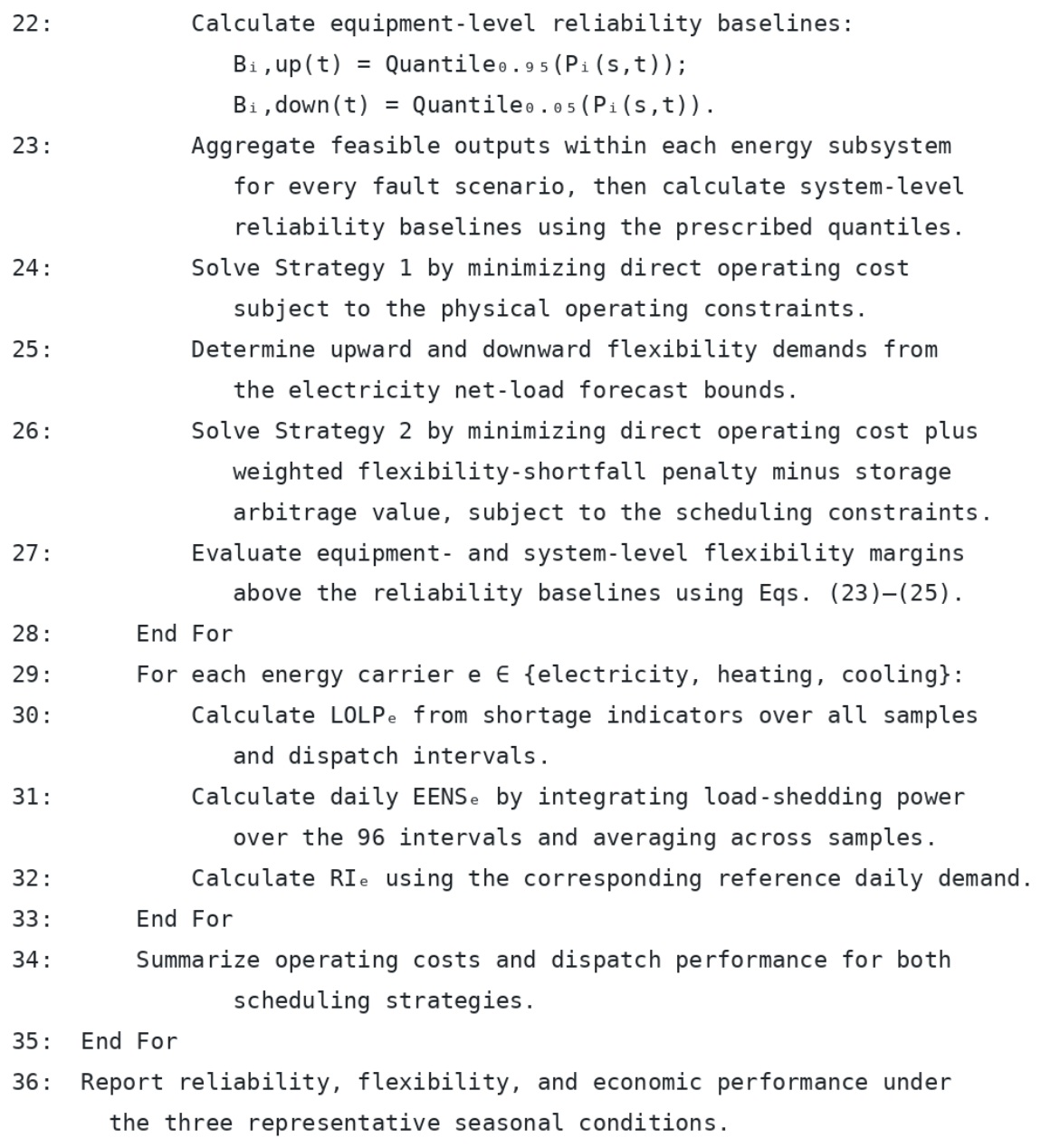
In this study, detailed unit commitment constraints, including startup and shutdown costs, minimum up-time, and minimum down-time constraints, are not considered. The energy conversion equipment is assumed to operate continuously within its allowable output range during the scheduling horizon. The operating constraints mainly focus on output limits and ramping capability. The overall workflow of the proposed framework is summarized in Appendix B. Figure A13 illustrates the reliability simulation and dynamic reliability baseline construction, while Figure A14 presents the scheduling optimization and performance evaluation procedure.
3. Case Study and Parameter Setting
To verify the effectiveness of the proposed strategy in improving overall system performance, this section compares an economic-only benchmark strategy (Strategy 1) with the proposed strategy considering both reliability and flexibility (Strategy 2). Simulations are conducted for typical winter, transition season, and summer days to reveal the differences between the two strategies in economic performance, equipment dispatch behaviors, and flexibility margin maintenance.
Strategy 1 represents the conventional economic-only benchmark, in which the flexibility penalty and arbitrage terms are disabled, and only direct operating costs are minimized under the specified single-period physical operating constraints.
Strategy 2 employs the same installed equipment configuration, load profiles, and physical resource limits, while incorporating flexibility shortfall penalties and energy-storage arbitrage value into the scheduling objective.
Both strategies are implemented through 15 min single-period dispatch calculations. Therefore, the optimization scope is restricted to each individual dispatch interval, rather than a jointly optimized 24 h scheduling problem. Strategy 1 is regarded as the economic-only benchmark solution under its specified objective and operating constraints. Global optimality is claimed only for individual subproblems for which the solver provides an optimal termination certificate. The reported seasonal results are obtained by aggregating the corresponding dispatch outcomes.
A data center in Lingang, Shanghai, is selected as the reference case in this study. The system configuration and operating scenario are established based on the actual characteristics of the data center campus. However, detailed equipment parameters and measured operational data of the facility involve commercial confidentiality and therefore cannot be publicly disclosed or directly used for validation. Accordingly, a simulation-based case study approach is adopted. Based on the building configuration, functional zoning, regional meteorological conditions, and energy-use characteristics of the reference data center, a building-energy model is established using DeST. The electricity, cooling, and heating load profiles for typical winter, transition season, and summer days are subsequently generated by the DeST model and used as inputs for the reliability assessment and scheduling optimization. Therefore, the case study should be interpreted as an actual-scenario-based simulation rather than a direct validation against measured operational data.
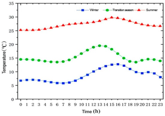
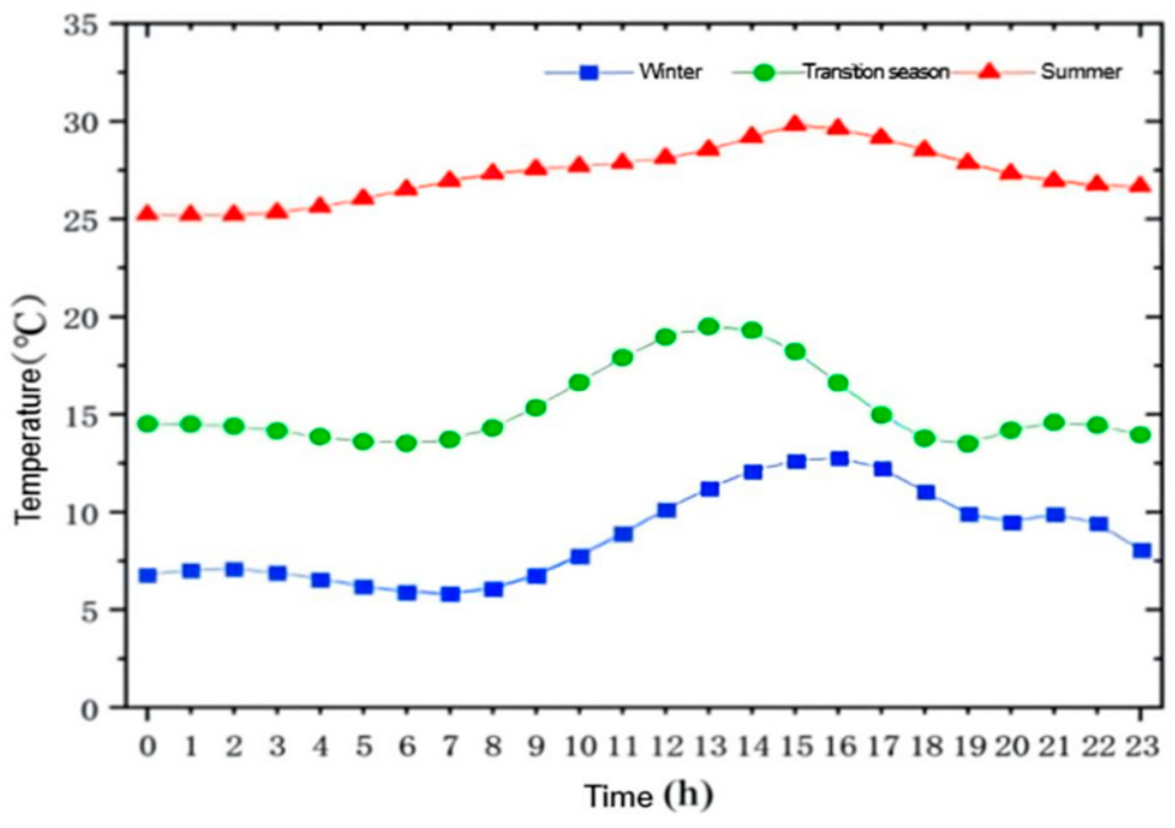
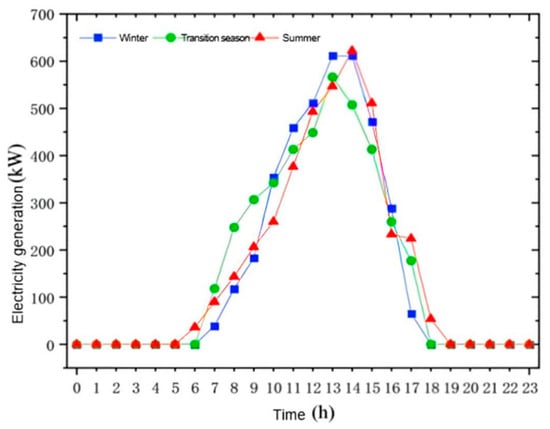
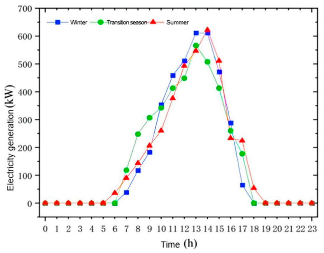
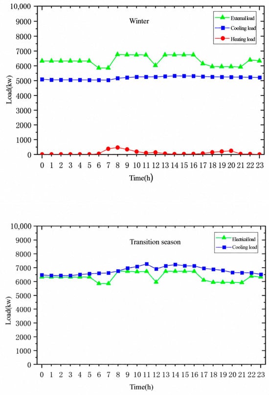
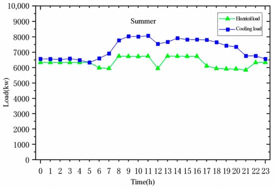
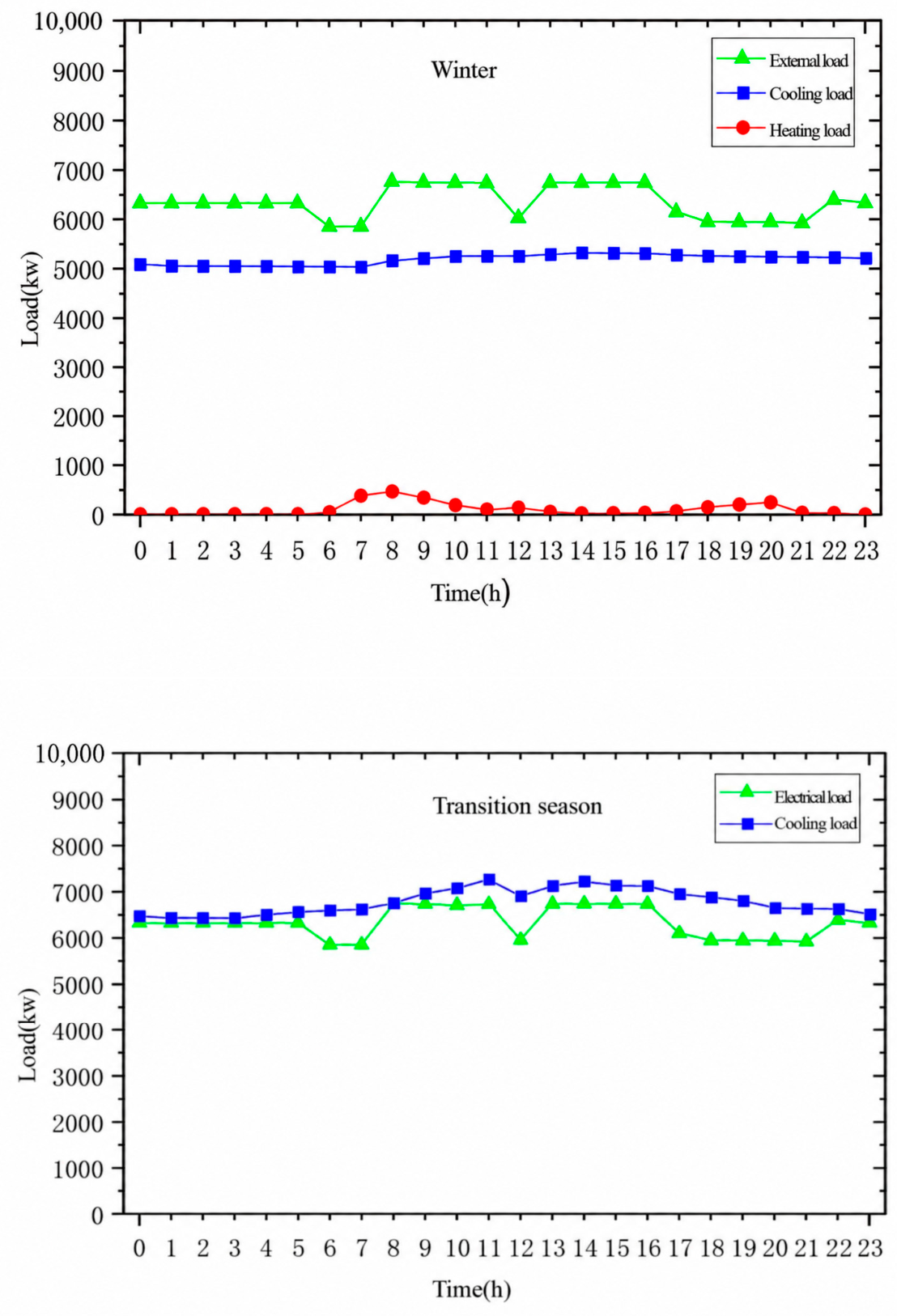
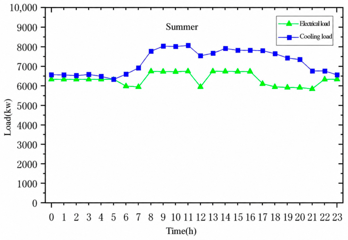
In addition, the photovoltaic generation profiles under different seasonal conditions are generated according to the regional solar radiation characteristics and the installed photovoltaic capacity of the reference data center. The photovoltaic output is considered as a predefined renewable energy input in the case study to represent the renewable energy availability under different operating conditions. It is not treated as an independent optimization decision variable in the reliability–flexibility coordinated scheduling model. The typical daily ambient temperature profiles for different seasons are shown in Figure 3, the corresponding seasonal photovoltaic generation profiles are presented in Figure 4, and the multi-energy load profiles are illustrated in Figure 5.
Figure 3.
Typical daily ambient temperature profiles for different seasons.
Figure 4.
PV output profiles for different seasons.
Figure 5.
Seasonal multi-energy load profiles.
The technical parameters of the multi-energy conversion equipment and energy storage systems are obtained from manufacturer specifications and the existing literature. The economic parameters are determined according to relevant market information and engineering assumptions. For economic parameters, the natural gas purchase price is set according to the current industrial gas price in Shanghai, which is 3.15 yuan/m3. The electricity purchase price follows a time-of-use tariff. For summer conditions, the peak, flat, and valley prices are 1.088, 0.66, and 0.245 yuan/kWh, respectively. For other seasons, the corresponding prices are 1.046, 0.618, and 0.304 yuan/kWh. The electricity export prices are set as 0.9, 0.55, and 0.35 yuan/kWh during peak, flat, and valley periods, respectively. The carbon emission cost is calculated using a carbon price of 0.1 yuan/kg, with emission factors of 0.38 kg/kWh for grid electricity and 0.4 kg/kWh for gas-fired generation. The operating parameters and life-cycle economic parameters of the core components within the multi-energy coupled architecture are summarized in Table 1, Table 2 and Table 3.
Table 1.
Parameters of energy supply equipment.
Table 2.
Investment and O&M cost parameters of energy supply units.
Table 3.
Operating parameters of energy supply units.
Due to confidentiality and availability limitations, these parameters are not directly obtained from site records. Instead, representative values are selected based on engineering assumptions and commonly reported reliability ranges of similar equipment.
In the reliability assessment process, Monte Carlo sampling is employed to generate stochastic equipment failure scenarios. The optimization model is implemented in MATLAB R2023b using YALMIP and solved with the CPLEX solver. Default solver termination criteria are adopted. The scheduling problem is formulated as a mixed-integer optimization problem. A 24 h scheduling horizon with a 15 min time resolution is adopted, resulting in 96 dispatch intervals for each representative day. The reliability sampling is performed separately before the scheduling optimization. The sampled equipment states are used for reliability assessment and dynamic reliability baseline construction, rather than being sampled endogenously within the optimization process. The chronological simulation is performed over a fixed two-year horizon. The generated equipment state trajectories are subsequently used for reliability evaluation. For the case study, the equipment states corresponding to representative winter, transition season, and summer operating days are extracted from the generated chronological trajectories. Reliability indices are evaluated separately for each seasonal condition, with 96 dispatch intervals per representative day. The uncertainty factors considered in this study include renewable energy fluctuations, load variations, and stochastic equipment failures. However, only equipment failures are modeled through stochastic sampling in the sequential Monte Carlo simulation. Among these uncertainties, stochastic sampling is explicitly applied only to equipment failures through the sequential Monte Carlo simulation. Photovoltaic output and load variations are represented by season-specific typical-day profiles and corresponding forecast ranges rather than by independent probability distributions. Winter, transition season, and summer operating conditions are modeled separately to reflect seasonal differences. Correlations between photovoltaic and load forecast errors are not explicitly considered in the present model. The generated scenarios are subsequently incorporated into the dynamic reliability baseline calculation and optimal scheduling process.
4. Result Analysis
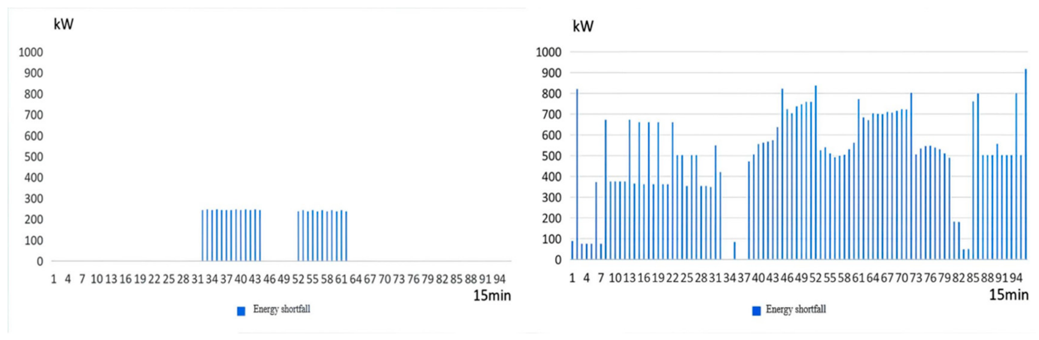
Figures for winter, summer, and the transition season present the same categories of results and have similar layouts. Therefore, only the summer results are presented in the main text, while winter and transition-season results are provided in Appendix A, Figure A1, Figure A2, Figure A3, Figure A4, Figure A5, Figure A6, Figure A7, Figure A8, Figure A9, Figure A10, Figure A11 and Figure A12.
- Power system comparison
The seasonal reliability assessment results of the power system under Strategy 1 and Strategy 2 are summarized in Table 4.
Table 4.
Reliability assessment results of the power system.
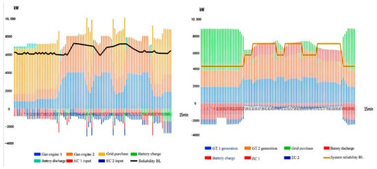
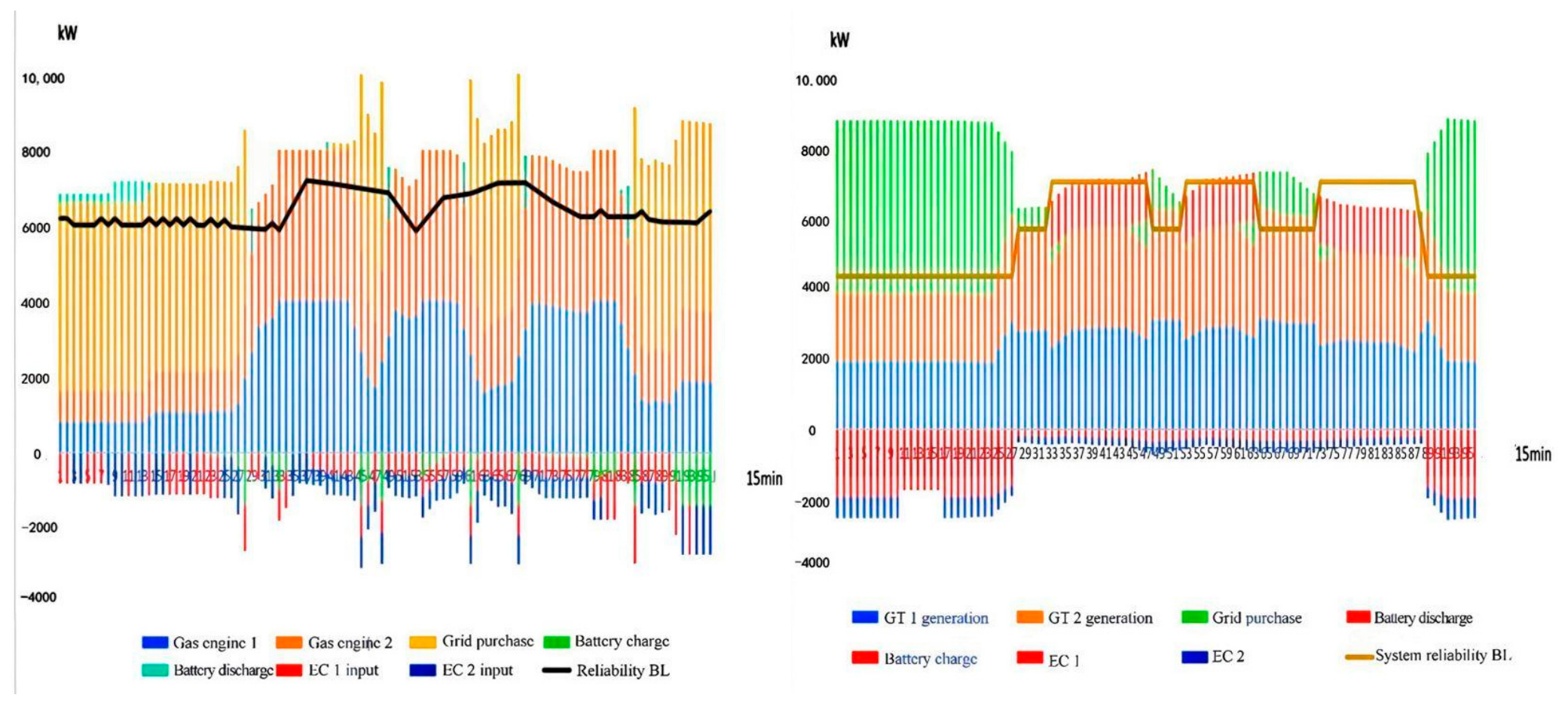
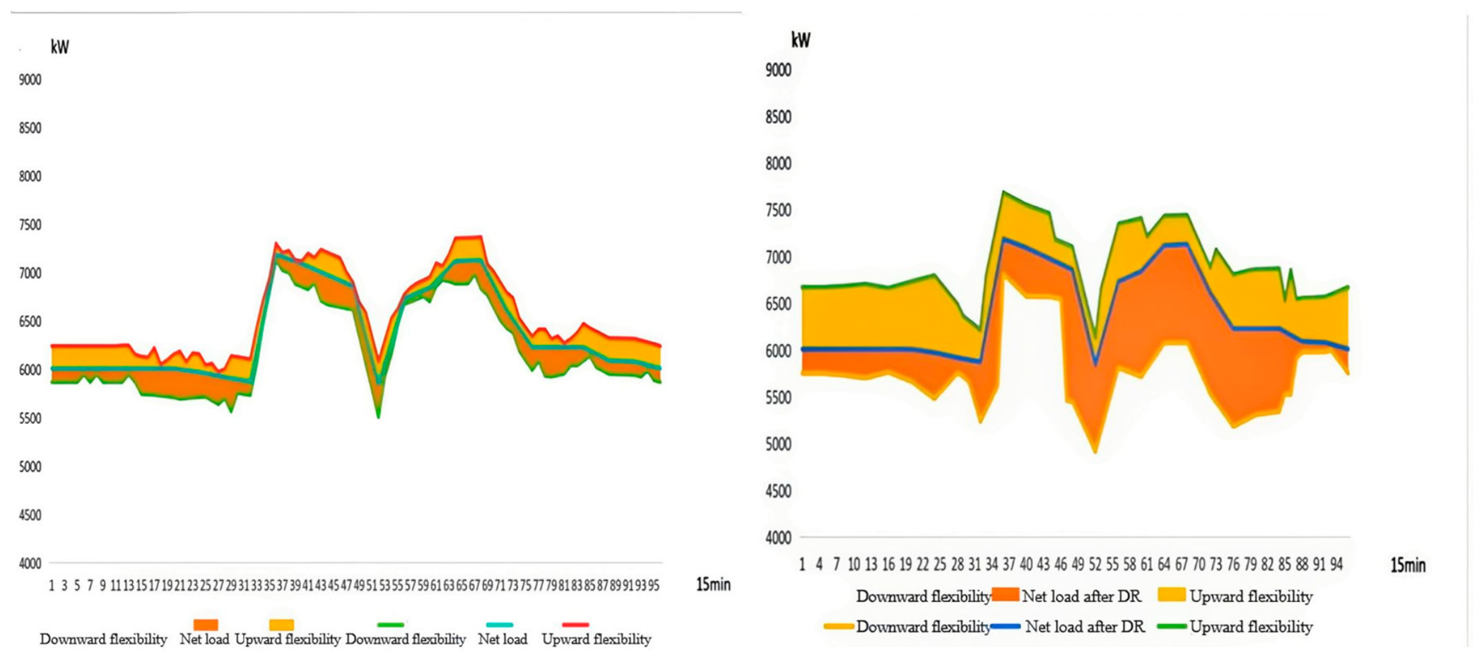
As shown in Figure 6 and Figure 7, the two strategies differ significantly in their power system operation modes. Strategy 1 tends to keep the gas engine operating at a high output level for extended periods, thereby improving equipment utilization and reducing electricity purchase costs. However, this operation mode results in insufficient adjustable capacity, with the flexibility margin approaching zero on multiple occasions during peak load periods. When the renewable energy output fluctuates or equipment failures occur, the system lacks sufficient reserve capacity for rapid response, thereby increasing the energy supply risk.
Figure 6.
Summer typical-day power system equipment dispatch and reliability baseline ((left): Strategy 1; (right): Strategy 2).
Figure 7.
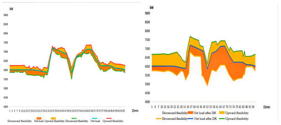
Summer typical-day flexibility margin above the reliability baseline of the power system ((left): Strategy 1; (right): Strategy 2).
In contrast, with the introduction of the dynamic reliability baseline and flexibility coordination mechanism, Strategy 2 no longer operates the gas engine continuously near its rated output. Instead, it proactively reserves a portion of its capacity to cope with potential fault scenarios. Meanwhile, the energy storage system, through coordinated charging and discharging during peak and off-peak periods, maintains relatively high upward and downward flexibility margins. When load increases or equipment failures occur, the reserved capacity can be rapidly released, effectively mitigating the supply–demand imbalance. As can be observed from Figure 7, Strategy 2 maintains a relatively stable flexibility level throughout the daily operation, indicating that the proposed reliability baseline can effectively guide the system in rationally allocating reserve resources.
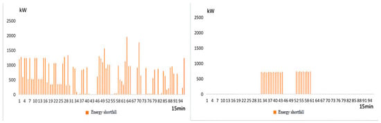
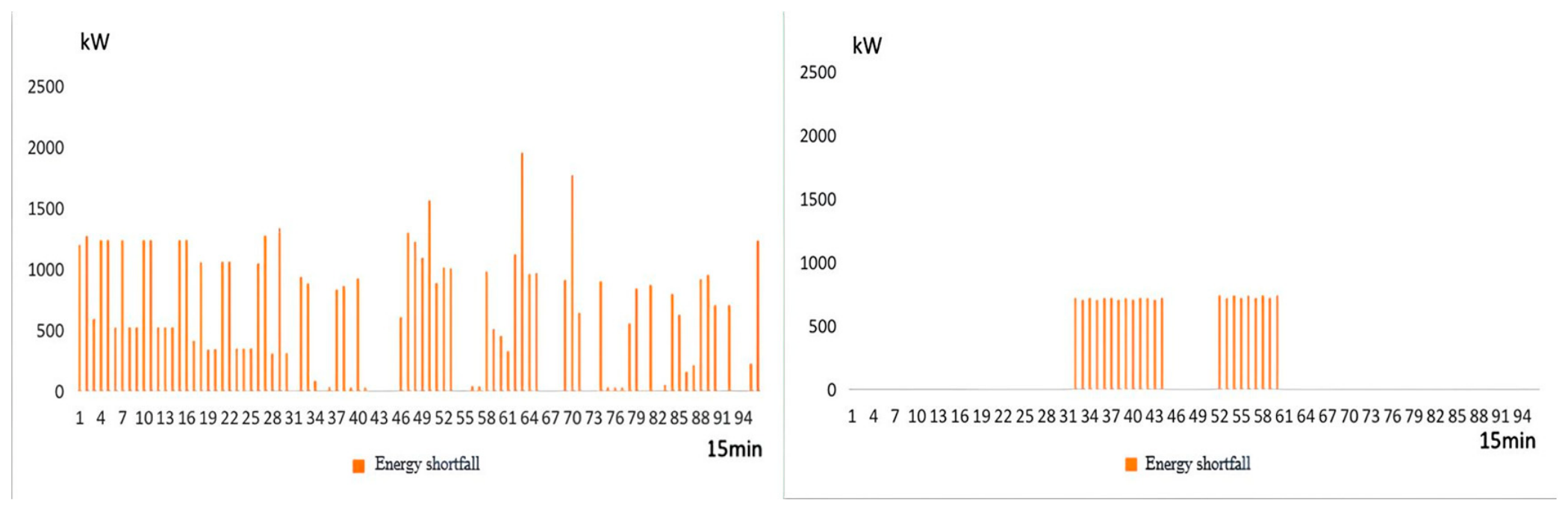
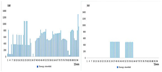
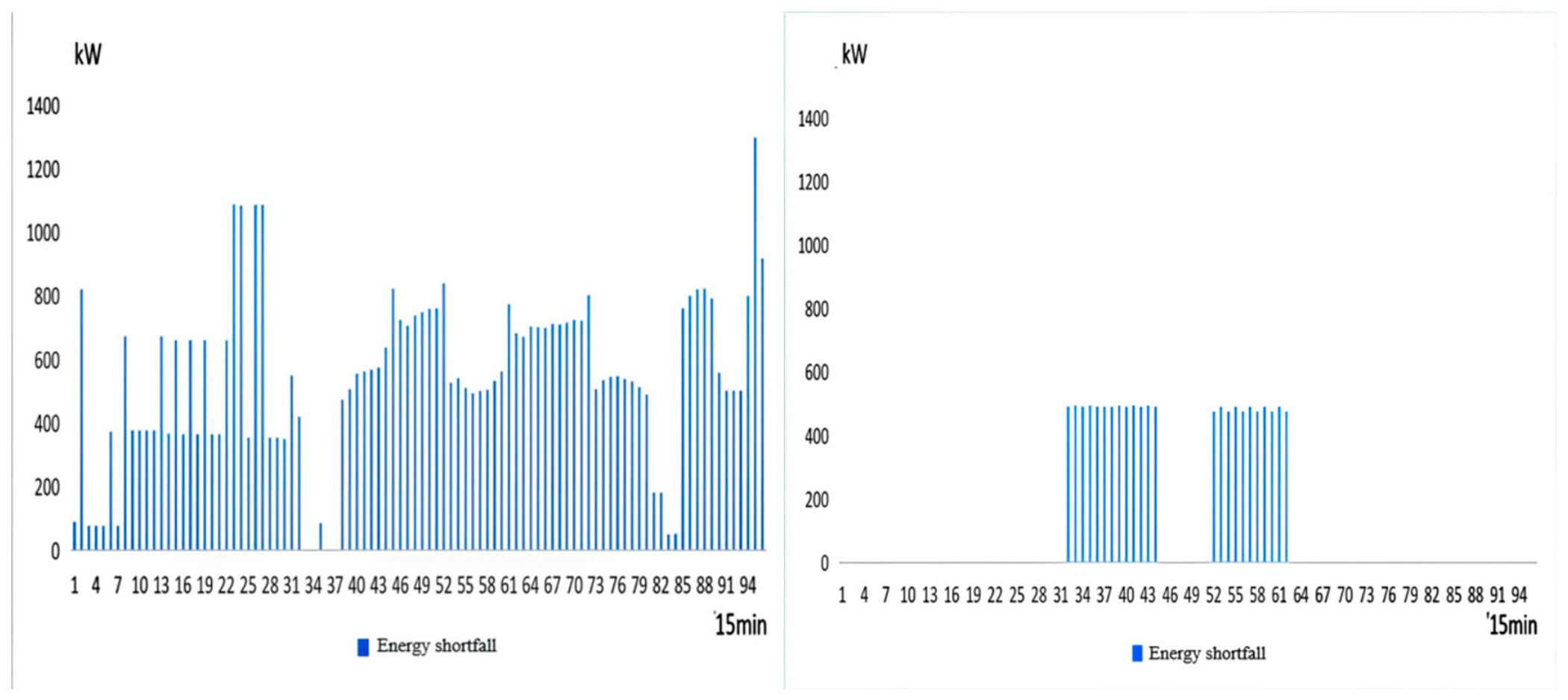
According to Figure 8 and Table 4, Strategy 2 significantly reduces the risk of energy supply shortfall under fault scenarios. Under typical summer conditions, the LOLP of the power system decreases from 0.029% to 0.016%, and the EENS decreases from 785.11 kWh to 227.36 kWh, representing a reduction of 71.0%. These results demonstrate that by reserving reliability capacity and maintaining sufficient flexibility margins, the system can effectively enhance its resilience to source load fluctuations and equipment failures, thereby improving the energy supply reliability index under an identical reference demand.
Figure 8.
Summer typical-day maximum power shortfall of the power system under fault conditions ((left): Strategy 1; (right): Strategy 2).
It should be noted that the zero flexibility shortfall penalty and load shedding penalty in Strategy 2 are obtained from the optimization results rather than manually assigned. The EENS values are calculated separately through the stochastic reliability assessment under equipment failure scenarios, whereas the load shedding penalty represents intentional load shedding within the deterministic scheduling optimization. Therefore, positive EENS values and zero load shedding penalty values are not contradictory because they describe different evaluation processes. The proposed reliability–flexibility coordinated scheduling strategy maintains sufficient operational reserves during the scheduling horizon, thereby avoiding scheduled flexibility violations and intentional load shedding.
The zero system-level LOLP, EENS, or flexibility shortfall values do not indicate that component failures or repairs are absent. The component failure and repair rates remain non-zero according to Table 3. Because the system includes two gas engines, multiple cooling units, the external power grid, and energy storage devices, the failure of a single component can usually be compensated for by the remaining supply units. Therefore, a component failure may occur without causing a system-level loss-of-load event.
- (1)
- Cooling system comparison
The seasonal reliability assessment results of the cooling system under the two scheduling strategies are summarized in Table 5.
Table 5.
Reliability assessment results of the cooling system.
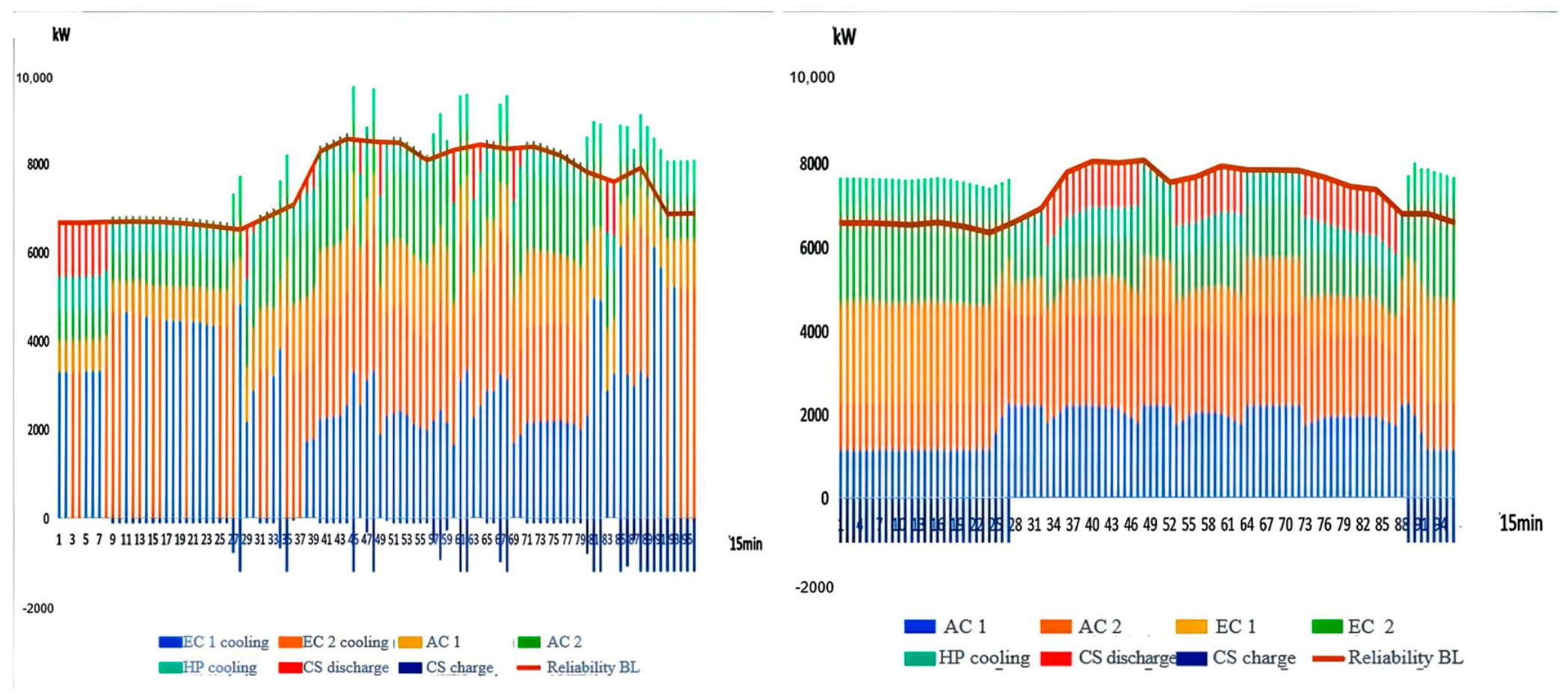
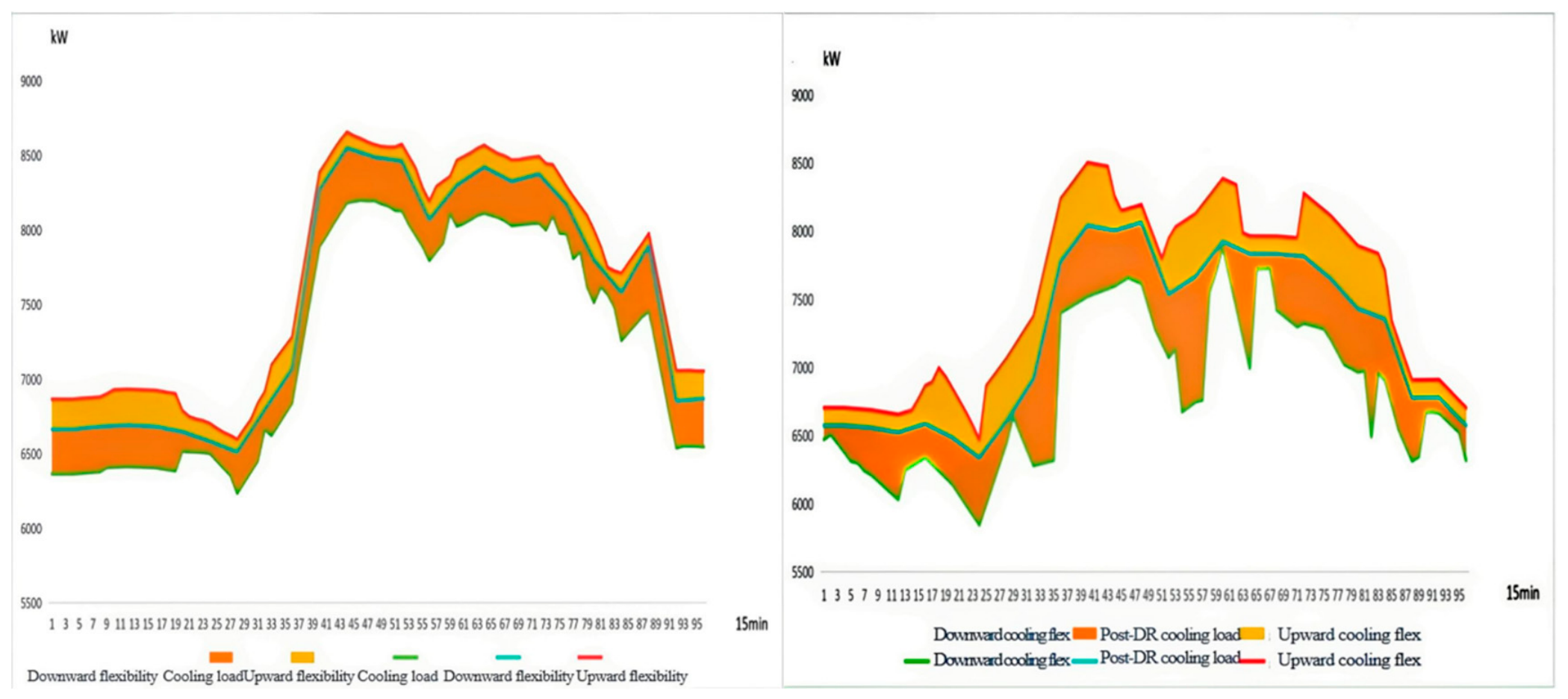
The cooling system is crucial for ensuring the safe and stable operation of a data center, as its reliability directly affects the operating environment of servers. As shown in Figure 9 and Figure 10, Strategy 1 relies primarily on electric chillers to undertake the base-load cooling task. Although this approach achieves relatively high equipment utilization, the overall reserve capacity of the system remains weak. When the cooling load increases rapidly or key equipment fails, the system is prone to insufficient cooling capacity.
Figure 9.
Summer typical-day cooling-system equipment dispatch and reliability baseline ((left): Strategy 1; (right): Strategy 2).
Figure 10.
Summer typical-day flexibility margin above the reliability baseline of the cooling system ((left): Strategy 1; (right): Strategy 2).
With the introduction of the dynamic reliability baseline, Strategy 2 further strengthens the coordinated operation among the electric chiller, the absorption chiller, and the cold storage device. The system reserves a portion of cooling capacity based on reliability requirements and fully utilizes the cold storage device to achieve cooling energy time shifting. When peak loads or equipment failures occur, the cold storage device can rapidly release cooling energy, while the absorption chiller utilizes waste heat resources to provide additional cooling support, thereby effectively improving the continuity of the cooling supply and fault recovery capability.
As shown in Figure 11 and Table 5, Strategy 2 significantly reduces the cooling supply shortfall under fault scenarios. Under summer conditions, the LOLP of the cooling system decreases from 0.028% to 0.015%, and the EENS decreases from 863.75 kWh to 152.13 kWh, representing a reduction of 82.3%. Because the cooling load in summer is at its highest level of the year and the operating margin is the smallest, the advantages of the synergy between the reliability baseline and flexibility margin are most pronounced. The results indicate that the proposed method can effectively enhance the cooling supply reliability of the data center integrated energy system under high-load operating conditions.The power shortfall shown in Figure 8 and Figure 11 represents the instantaneous power deficit observed in sampled fault scenarios. These figures illustrate the magnitude of insufficient-supply events and do not define the reliability baseline. The maximum power shortfall reflects the severity of individual scenarios at specific intervals. In contrast, EENS measures the expected accumulated unserved energy over the representative day (kWh/day), calculated by integrating curtailed power over the 15 min intervals and averaging across sampled scenarios. Thus, maximum power shortfall describes the worst-case deficit, whereas EENS captures the expected unserved energy across scenarios.
Figure 11.
Summer typical-day maximum power shortfall of the cooling system under fault conditions ((left): Strategy 1; (right): Strategy 2).
- (2)
- Economic performance analysis
In addition, because the heating load of the data center is relatively small, no energy supply shortfall occurs in the heating system under either strategy. Therefore, this study does not conduct a separate analysis of the heating system.
The reported total cost includes direct operating cost and reliability/flexibility-related penalty terms. Both strategies use the same accounting period and cost definitions for comparison.
As shown in Table 6, Strategy 2 exhibits lower direct operating costs than Strategy 1 under all three seasonal conditions, with reductions of 4.67%, 6.63%, and 1.82% for winter, transition season, and summer, respectively. When flexibility and load-shedding penalties are included, the corresponding reductions in comprehensive accounted costs are 13.68%, 15.16%, and 10.93%. These results indicate differences in the operating-cost outcomes of the two implemented scheduling strategies. However, the lower direct operating costs of Strategy 2 should not be interpreted as proof of superiority over a certified global optimum of the economic-only formulation. The comparison is based on the numerical solutions obtained under the respective implemented scheduling procedures.
Table 6.
Summary of system operating costs.
In addition, the carbon emission treatment cost considered in this study represents the economic impact of carbon emissions rather than a direct measurement of greenhouse gas emissions. Although flexible scheduling can improve renewable energy accommodation and energy utilization efficiency, its quantitative carbon reduction potential depends on the energy supply structure and carbon intensity information. Due to the lack of mature dynamic carbon emission factor models, further carbon-aware scheduling based on real-time carbon signals will be investigated in future studies.
- (3)
- Sensitivity and Sampling Uncertainty Analysis
A preliminary test of the flexibility shortfall penalty coefficient showed negligible changes in the scheduling results. Therefore, electricity and natural gas prices were selected for further one-factor-at-a-time sensitivity analysis. Each price was varied by −20%, −10%, 0%, +10%, and +20% relative to its baseline value, while all other parameters remained unchanged. Because the case study uses representative seasonal operating days rather than continuous annual measurements, the economic results are expressed as equivalent annual costs. A non-leap year is divided into three seasonal periods: 90 winter days, 183 transition-season days, and 92 summer days.
As shown in Table 7, electricity price variations from −20% to +20% result in annual operating costs ranging from 52.54 million to 57.46 million RMB, corresponding to changes of approximately −4.87% to +4.04%. Natural gas price variations produce a larger cost change, ranging from 46.57 million to 63.02 million RMB (−15.68% to +14.10%). These results indicate that the system operating cost is more sensitive to natural gas prices than to electricity prices.
Table 7.
Equivalent annual direct operating cost under electricity- and natural-gas-price perturbations.
To quantify the sampling uncertainty of the reliability estimates, nonparametric bootstrap replications are performed using the original Monte Carlo trajectories. The 95% confidence intervals are obtained from the 2.5th and 97.5th percentiles of the bootstrap estimates. As shown in Table 8, the confidence intervals vary across the electricity, heating, and cooling subsystems. The relatively wide intervals for some indices reflect the limited number of observed shortage events, highlighting the sampling uncertainty associated with the reliability estimates.
Table 8.
Sampling uncertainty of reliability indices.
5. Conclusions
To address the challenges of insufficient energy supply reliability and limited regulation capability in data center integrated energy systems under renewable energy fluctuations and stochastic equipment failures, this study proposes a reliability–flexibility coordinated optimal scheduling strategy based on dynamic reliability assessment and flexibility margins. The proposed framework provides an effective approach for improving energy supply reliability, operational flexibility, and economic performance. The main conclusions are summarized as follows:
- (1)
- A dynamic-reliability-oriented evaluation model for the distributed integrated energy system is established. By developing key equipment models for the gas engine, electric chiller, absorption chiller, and energy storage devices, and introducing a sequential Monte Carlo simulation based on a two-state Markov model method to characterize the state transition processes of equipment operation, a dynamic reliability assessment model applicable to the electricity and cooling of multi-energy systems is constructed. Based on the loss of load probability (LOLP) and expected energy not supplied (EENS), the quantitative evaluation of the system energy supply reliability is achieved.
- (2)
- A dynamic reliability baseline and flexibility margin model are proposed to coordinate reliability requirements and operational flexibility. By determining the minimum reserve capacity required under fault scenarios, the proposed method avoids excessive reliance on economic-oriented operation strategies and enables the system to maintain sufficient regulation capability while ensuring energy supply security.
- (3)
- An optimal scheduling framework considering dynamic reliability and flexibility coordination is developed. Compared with the conventional economic scheduling strategy, the proposed method significantly reduces energy supply risks and improves operational performance. Under typical summer conditions, the EENS of the power system decreases from 785.11 kWh to 227.36 kWh, while the EENS of the cooling system decreases from 863.75 kWh to 152.13 kWh, corresponding to reductions of 71.0% and 82.3%, respectively. Meanwhile, the total operating cost decreases by 13.68%, 15.16%, and 10.93% under winter, transition season, and summer conditions, respectively.
Several limitations should also be acknowledged. First, the proposed framework is demonstrated based on a single data center integrated energy system configuration, and the general applicability to other system configurations requires further validation. Second, the case study is conducted using representative seasonal operating days rather than continuous annual measured operation data. Therefore, these results should be interpreted as simulation-based evaluations under representative operating conditions rather than comprehensive long-term field validation.
Future research will focus on integrating dynamic carbon emission factors and carbon-aware scheduling mechanisms into the proposed reliability–flexibility framework. With the development of real-time carbon intensity monitoring and forecasting technologies, flexible resources such as energy storage and multi-energy conversion equipment can be further coordinated with carbon signals to better evaluate potential emission-reduction benefits. Meanwhile, the sustainable transformation of data centers should also be investigated from the perspective of system configuration, including renewable energy deployment, energy storage planning, and low-carbon energy supply architectures.
Author Contributions
Conceptualization, L.Z.; methodology, L.Z. and S.L.; software, L.Z. and L.S.; validation, X.X., L.S. and Q.L.; formal analysis, L.Z., S.L., F.Q. and Y.Y.; resources, L.Z. and X.X.; data curation, L.Z., F.Q. and Y.Y.; writing—original draft preparation, L.Z., S.L. and Y.Y.; writing—review and editing, L.Z. and S.L.; visualization, S.L. and X.X.; supervision, F.Q. and Q.L. All authors have read and agreed to the published version of the manuscript.
Funding
Project supported by the Young Scientists Fund of the National Natural Science Foundation of China (No. 52308110).
Institutional Review Board Statement
Not applicable.
Informed Consent Statement
Not applicable.
Data Availability Statement
The detailed operational data and equipment parameters of the reference data center are not publicly available due to commercial confidentiality restrictions. The load profiles used in this study were generated using the DeST building-energy simulation model based on the building configuration, regional meteorological conditions, and energy-use characteristics of the reference data center. The model parameters and representative simulation results necessary to understand the methodology are provided in the manuscript. The original confidential facility data cannot be shared.
Conflicts of Interest
The authors declare no conflict of interest.
Appendix A
Figure A1.
Winter typical-day power system equipment dispatch and reliability baseline ((left): Strategy 1; (right): Strategy 2).
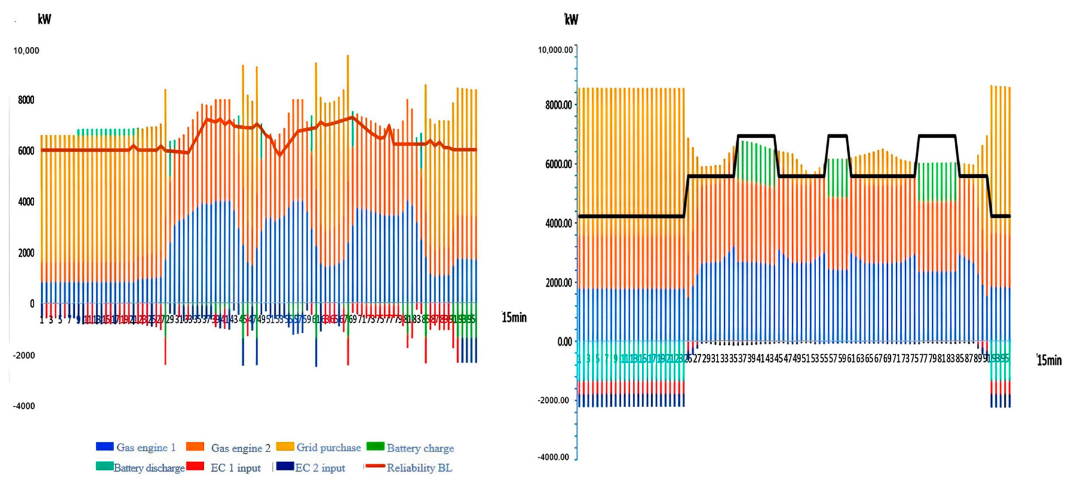
Figure A2.
Winter typical-day flexibility margin above the reliability baseline of the power system ((left): Strategy 1; (right): Strategy 2).
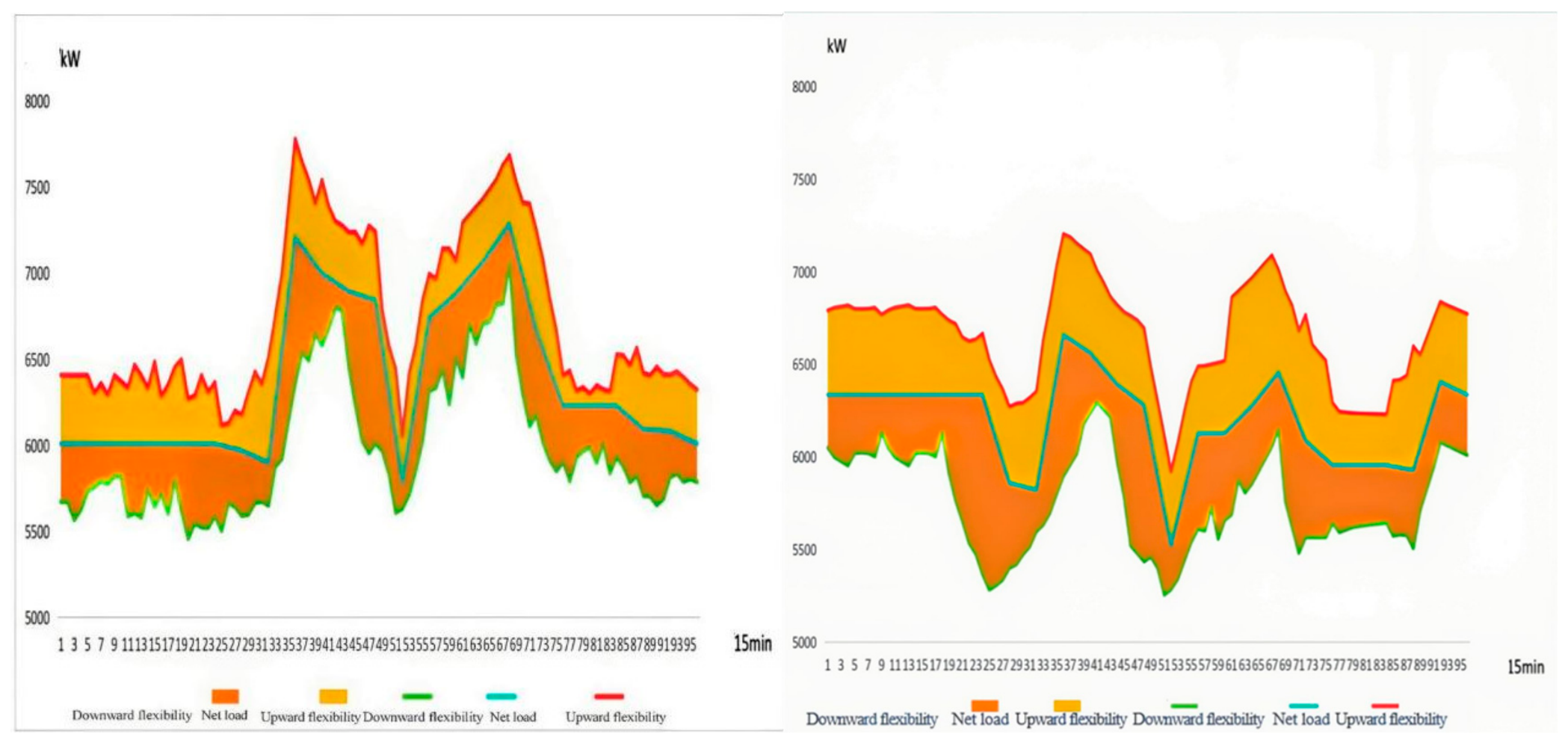
Figure A3.
Winter typical-day maximum power shortfall of the power system under fault conditions ((left): Strategy 1; (right): Strategy 2).
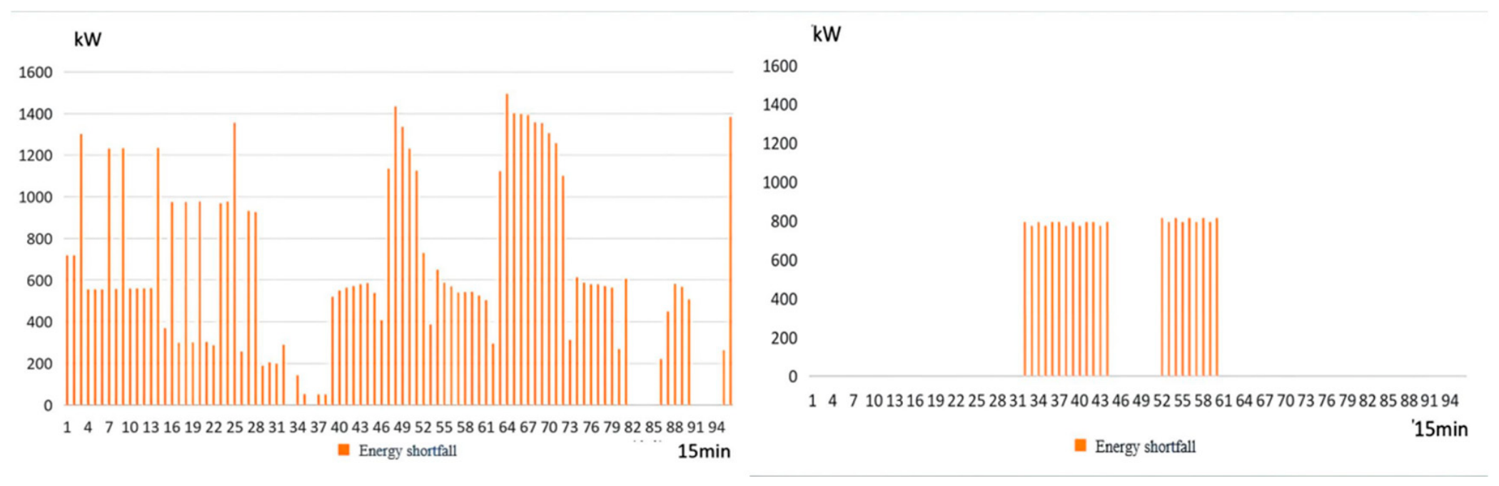
Figure A4.
Transition season typical-day power system equipment dispatch and reliability baseline ((left): Strategy 1; (right): Strategy 2).
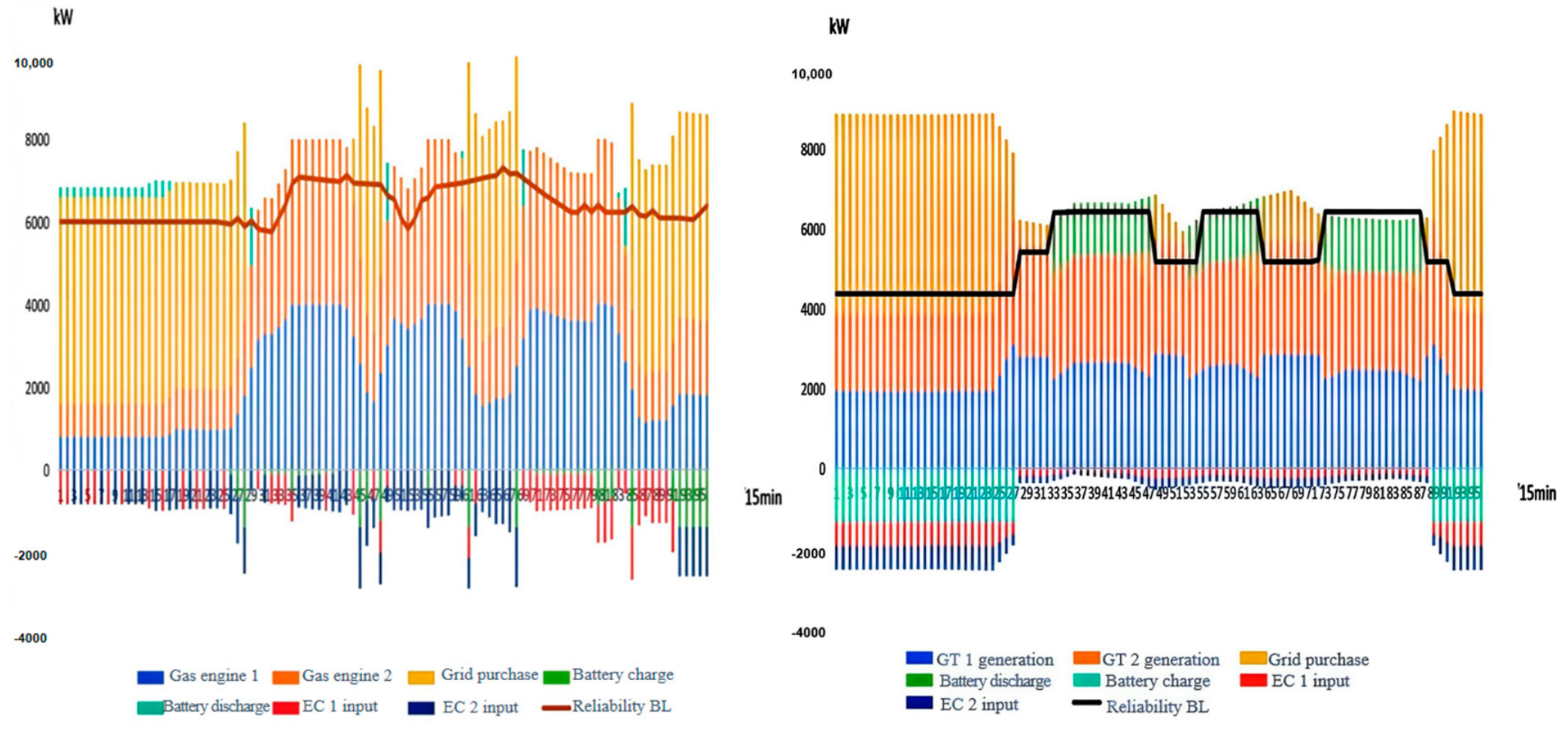
Figure A5.
Transition season typical-day flexibility margin above the reliability baseline of the power system ((left): Strategy 1; (right): Strategy 2).
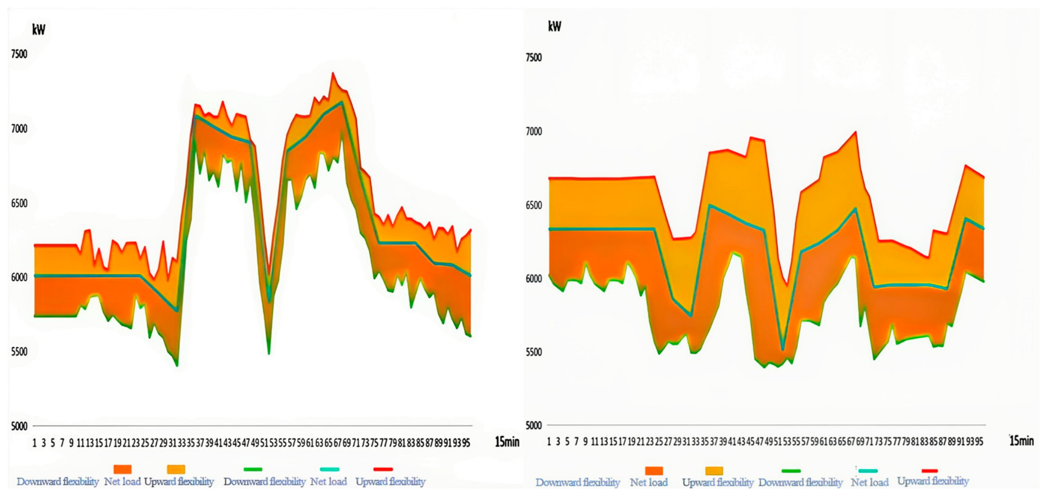
Figure A6.
Transition season typical-day maximum power shortfall of the power system under fault conditions ((left): Strategy 1; (right): Strategy 2).
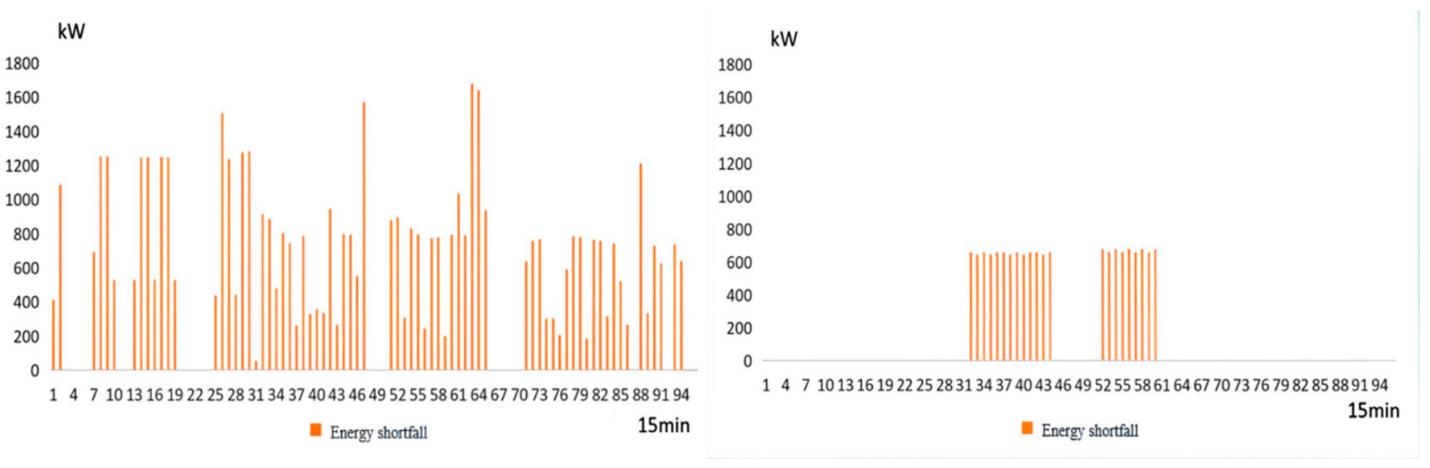
Figure A7.
Winter typical-day cooling system equipment dispatch and reliability baseline ((left): Strategy 1; (right): Strategy 2).
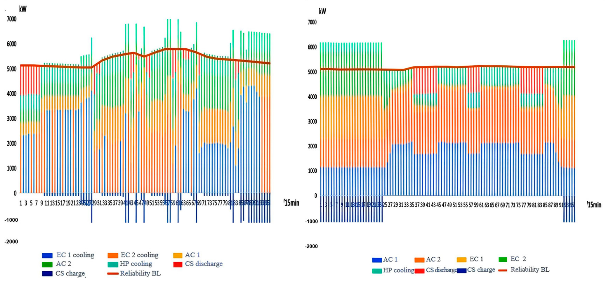
Figure A8.
Winter typical-day flexibility margin above the reliability baseline of the cooling system ((left): Strategy 1; (right): Strategy 2).
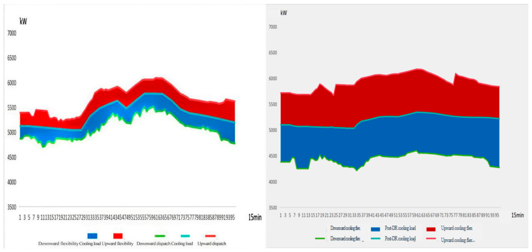
Figure A9.
Winter typical-day maximum power shortfall of the cooling system under fault conditions ((left): Strategy 1; (right): Strategy 2).
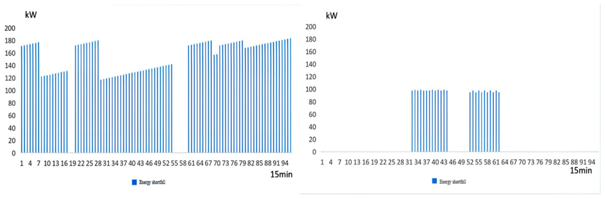
Figure A10.
Transition season typical-day cooling system equipment dispatch and reliability baseline ((left): Strategy 1; (right): Strategy 2).
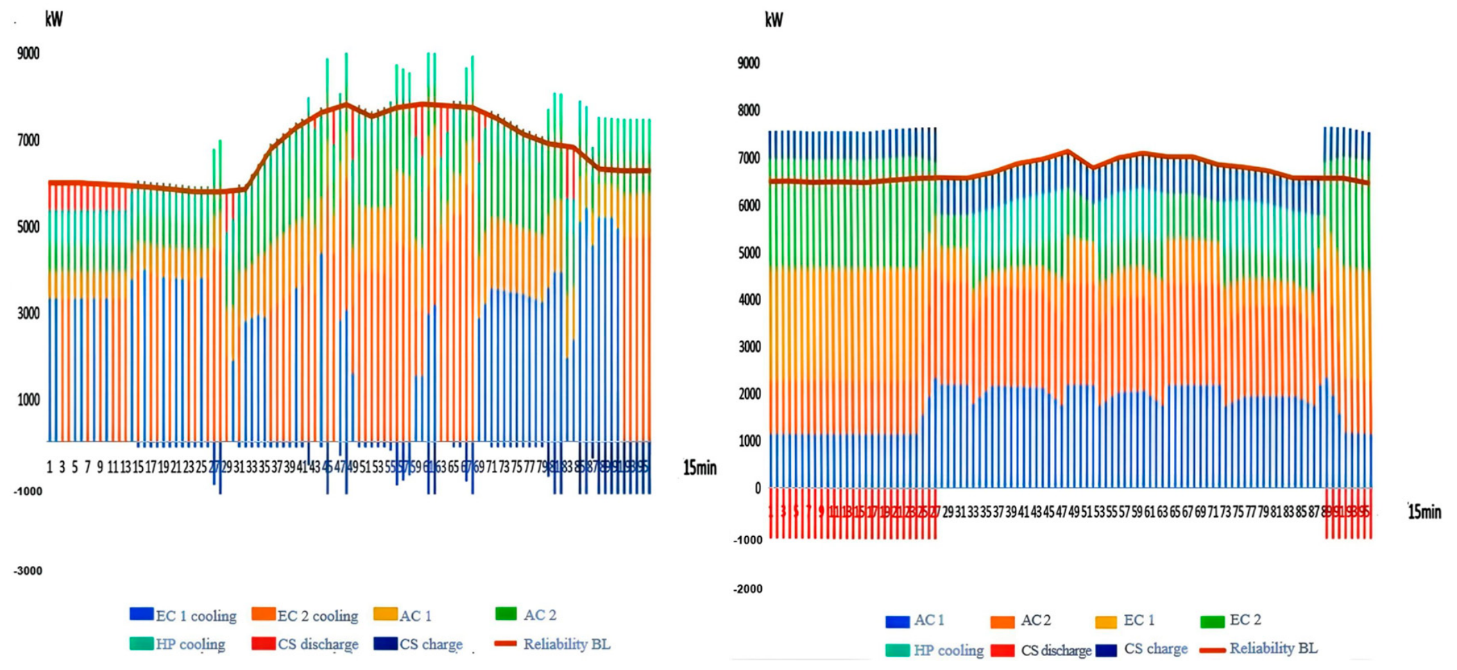
Figure A11.
Transition season typical-day flexibility margin above the reliability baseline of the cooling system ((left): Strategy 1; (right): Strategy 2).
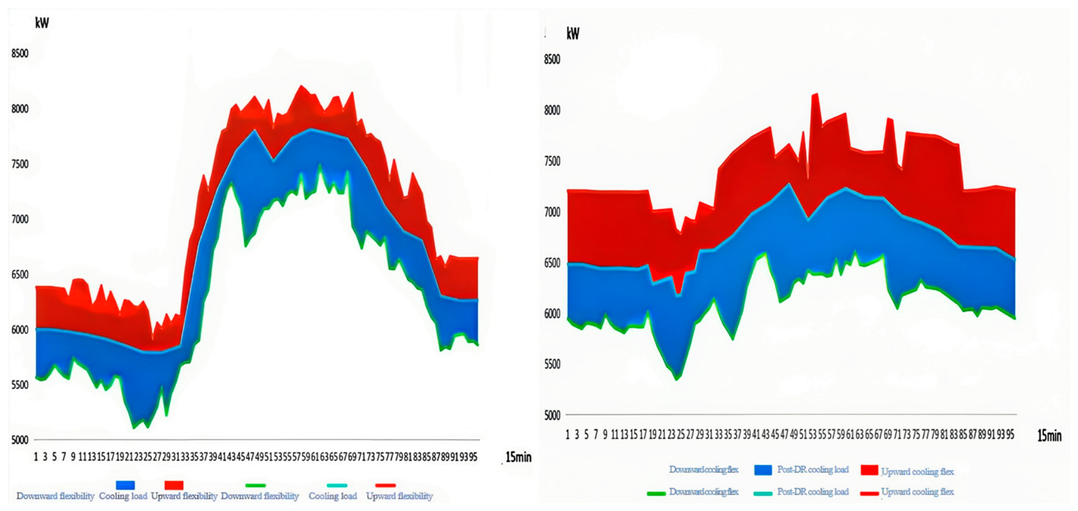
Figure A12.
Transition season typical-day maximum power shortfall of the cooling system under fault conditions ((left): Strategy 1; (right): Strategy 2).
Appendix B
Figure A13.
Reliability Simulation and Baseline Construction.
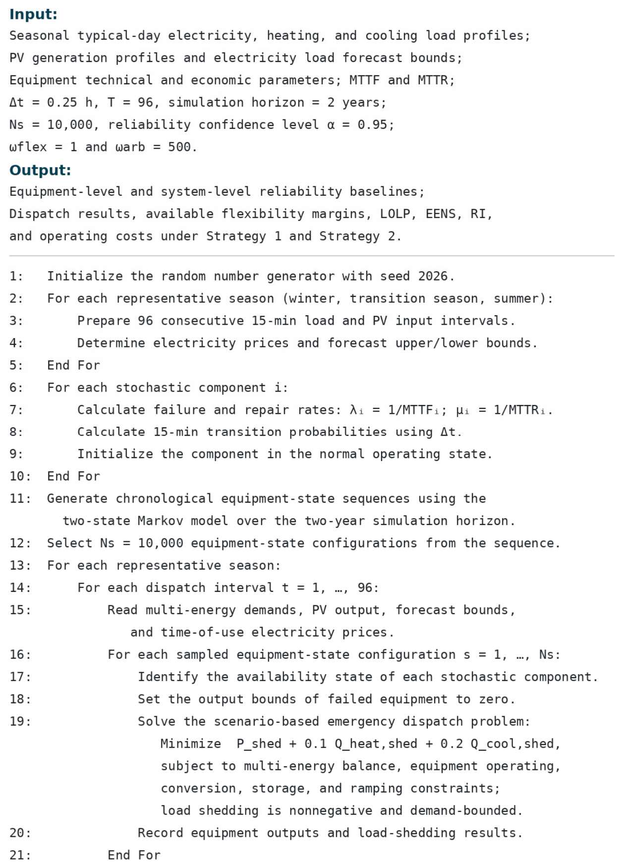
Figure A14.
Scheduling Optimization and Performance Evaluation.
References
- Tahir, M.; Hu, S.; Zhu, H. Advanced levelized cost evaluation method for electric vehicle stations concurrently producing electricity and hydrogen. Energies 2024, 17, 2682. [Google Scholar] [CrossRef] [Scilit]
- Thirunavukkarasu, M.; Sawle, Y.; Lala, H. A Comprehensive Review on Optimization of Hybrid Renewable Energy Systems Using Various Optimization Techniques. Renew. Sustain. Energy Rev. 2023, 176, 113192. [Google Scholar] [CrossRef] [Scilit]
- Elomari, Y.; Aspetakis, G.; Mateu, C.; Shobo, A.; Boer, D.; Marín-Genescà, M.; Wang, Q. A hybrid data-driven co-simulation approach for enhanced integrations of renewables and thermal storage in building district energy systems. J. Build. Eng. 2025, 104, 112405. [Google Scholar] [CrossRef] [Scilit]
- Pan, L.; Wang, Y.; Ding, Y. Integrated energy system scheduling strategy for zero-energy buildings based on MC-TD3 algorithm. J. Build. Eng. 2025, 111, 112920. [Google Scholar] [CrossRef] [Scilit]
- Tian, C.; Zhang, H.; Ma, X.; Li, M.; Yan, A.; Liu, Q. Enhancing the feasible region of building scale integrated energy systems via feature fusion prediction and complementary scheduling. J. Build. Eng. 2026, 119, 115340. [Google Scholar] [CrossRef] [Scilit]
- Bhuiyan, F.A.; Yazdani, A. Reliability assessment of a wind-power system with integrated energy storage. IET Renew. Power Gener. 2010, 4, 211–220. [Google Scholar] [CrossRef] [Scilit]
- Chi, L.; Su, H.; Zio, E.; Qadrdan, M.; Li, X.; Zhang, L.; Fan, L.; Zhou, J.; Yang, Z.; Zhang, J. Data-driven reliability assessment method of integrated energy systems based on probabilistic deep learning and Gaussian mixture model-hidden Markov model. Renew. Energy 2021, 174, 952–970. [Google Scholar] [CrossRef] [Scilit]
- Lei, Y.; Hou, K.; Wang, Y.; Jia, H.; Zhang, P.; Mu, Y.; Jin, X.; Sui, B. A new reliability assessment approach for integrated energy systems: Using hierarchical decoupling optimization framework and impact-increment based state enumeration method. Appl. Energy 2018, 210, 1237–1250. [Google Scholar] [CrossRef] [Scilit]
- Chen, J.; Yu, T.; Xu, Y.; Cheng, X.; Yang, B.; Zhen, B. Fast analytical method for reliability evaluation of electricity-gas integrated energy system considering dispatch strategies. Appl. Energy 2019, 242, 260–272. [Google Scholar] [CrossRef] [Scilit]
- Fu, X.; Guo, Q.; Sun, H.; Zhang, X.; Wang, L. Estimation of the failure probability of an integrated energy system based on the first order reliability method. Energy 2017, 134, 1068–1078. [Google Scholar] [CrossRef] [Scilit]
- Li, G.; Li, G.; Bie, Z.; Kou, Y.; Jiang, J.; Bettinelli, M. Reliability evaluation of integrated energy systems based on smart agent communication. Appl. Energy 2016, 167, 397–406. [Google Scholar] [CrossRef] [Scilit]
- Dai, W.; Zheng, H.; Shi, B.; Liu, H. Reliability evaluation of solar pavements-integrated power system considering seasonal meteorological factors and traffic road congestion. Appl. Energy 2026, 410, 127566. [Google Scholar] [CrossRef] [Scilit]
- Cao, M.; Shao, C.; Hu, B.; Xie, K.; Li, W.; Peng, L.; Zhang, W. Reliability Assessment of Integrated Energy Systems Considering Emergency Dispatch Based on Dynamic Optimal Energy Flow. IEEE Trans. Sustain. Energy 2021, 13, 290–301. [Google Scholar] [CrossRef] [Scilit]
- Fu, Y.; Sun, Q.; Wennersten, R.; Pang, X.; Liu, W. Uncertainty-Based System Flexibility Evaluation and Multi-Objective Collaborative Optimization of Integrated Energy System. Processes 2025, 13, 2047. [Google Scholar] [CrossRef] [Scilit]
- Qu, J.; Xu, K.; Hou, K.; Liu, Z.; Wu, H.; Jia, H.; Zhu, L. Reliable and economic operation of regional-community integrated energy systems: A hybrid game approach based on state similarity. Energy 2025, 336, 137983. [Google Scholar] [CrossRef] [Scilit]
- Ren, H.; Jiang, Z.; Wu, Q.; Li, Q.; Yang, Y. Integrated optimization of a regional integrated energy system with thermal energy storage considering both resilience and reliability. Energy 2022, 261, 125333. [Google Scholar] [CrossRef] [Scilit]
- International Energy Agency (IEA). Empowering Variable Renewables: Options for Flexible Electricity Systems; OECD Publishing: Paris, France, 2009. [Google Scholar]
- North American Electric Reliability Corporation (NERC). Special Report: Potential Reliability Impacts of Emerging Flexible Resources; NERC: Princeton, NJ, USA, 2010. [Google Scholar]
- Li, P.; Wang, Y.; Ji, H.; Zhao, J.; Song, G.; Wu, J.; Wang, C. Operational flexibility of activedistribution networks: Definition, quantified calculation and application. Int. J. Electr. Power Energy Syst. 2020, 119, 105872. [Google Scholar] [CrossRef] [Scilit]
- Chicco, G.; Riaz, S.; Mazza, A.; Mancarella, P. Flexibility From Distributed Multienergy Systems. Proc. IEEE 2020, 108, 1496–1517. [Google Scholar] [CrossRef] [Scilit]
- Zhang, N.; Chen, Y.; Deng, H.; Ma, T.; Zheng, S.; Zhang, Z. Flexibility-driven distributed coordination for low-carbon operation of active distribution networks with multi-park integrated energy systems. Appl. Energy 2026, 415, 127861. [Google Scholar] [CrossRef] [Scilit]
- Zhu, X.; Sun, Y.; Yang, J.; Dou, Z.; Li, G.; Xu, C.; Wen, Y. Day-ahead energy pricing and management method for regional integrated energy systems considering multi-energy demand responses. Energy 2022, 251, 123914. [Google Scholar] [CrossRef] [Scilit]
- Heggarty, T.; Bourmaud, J.-Y.; Girard, R.; Kariniotakis, G. Quantifying power system flexibility provision. Appl. Energy 2020, 279, 115852. [Google Scholar] [CrossRef] [Scilit]
- Xu, X.; Lyu, Q.; Qadrdan, M.; Wu, J. Quantification of Flexibility of a District Heating System for the Power Grid. IEEE Trans. Sustain. Energy 2020, 11, 2617–2630. [Google Scholar] [CrossRef] [Scilit]
- Haakana, J.; Haapaniemi, J.; Vilppo, J.; Lassila, J. Methodology to determine residential heating-based flexibility potential in electricity distribution networks. Sustain. Energy Grids Netw. 2022, 33, 100961. [Google Scholar] [CrossRef] [Scilit]
- Koltsaklis Nikolaos, E.; Knápek, J. Assessing flexibility options in electricity market clearing. Renew. Sustain. Energy Rev. 2023, 173, 11308468. [Google Scholar] [CrossRef] [Scilit]
- Digvijay, G.; Milos, C.; Peter, P. Quantification of operational flexibility from a portfolio of flexible energy resources. Int. J. Electr. Power Energy Syst. 2022, 141, 107466. [Google Scholar] [CrossRef] [Scilit]
- Akbari, E.; Shabestari, S.F.M.; Pirouzi, S.; Jadidoleslam, M. Network flexibility regulation by renewable energy hubs using flexibility pricing-based energy management. Renew. Energy 2023, 206, 295–308. [Google Scholar] [CrossRef] [Scilit]
- Zhang, S.; Ge, S.; Liu, H.; Zhao, B.; Ni, C.; Hou, G.; Wang, C. Region-based flexibility quantification in distribution systems: An analytical approach considering spatio-temporal coupling. Appl. Energy 2024, 355, 122175. [Google Scholar] [CrossRef] [Scilit]
- Huang, X.; Zhong, J.; Zhao, J.; Cao, Y.; Zeng, Z.; Feng, C. Risk-averse scheduling of integrated energy systems: Green-carbon market coordination with flexible resources. Energy 2026, 344, 139614. [Google Scholar] [CrossRef] [Scilit]
- Degefa, M.Z.; Sperstad, I.B.; Sæle, H. Comprehensive classifications and characterizations of power system flexibility resources. Electr. Power Syst. Res. 2021, 194, 107022. [Google Scholar] [CrossRef] [Scilit]

Disclaimer/Publisher’s Note: The statements, opinions and data contained in all publications are solely those of the individual author(s) and contributor(s) and not of MDPI and/or the editor(s). MDPI and/or the editor(s) disclaim responsibility for any injury to people or property resulting from any ideas, methods, instructions or products referred to in the content. |
© 2026 by the authors. Licensee MDPI, Basel, Switzerland. This article is an open access article distributed under the terms and conditions of the Creative Commons Attribution (CC BY) license.