Sustainability-Oriented Time-Varying Optimal Scheduling of Household Appliances Using Adaptive Multi-Source Transfer Algorithm

Abstract

Under the “dual carbon” strategy, home energy management systems have emerged as a core demand-side management technology to enable sustainable residential energy consumption. Nevertheless, most existing research investigates appliance scheduling within static frameworks. This study develops a dynamic three-objective scheduling model that minimizes electricity cost, user dissatisfaction, and carbon emissions. An adaptive multi-source transfer learning-assisted dynamic multi-objective evolutionary algorithm (AMS-TL-RMMEDA) is proposed to track the time-varying Pareto-optimal sets. The algorithm assigns transfer weights using Hausdorff-based similarity metrics, transfers historical knee points via geodesic flow kernel subspace alignment, and adjusts its response strategy according to quantified change intensity. On DF1–DF14, AMS-TL-RMMEDA yields the best MIGD values for 8 out of 14 problems and attains the lowest Friedman rank of 1.98. In simulations with eight household appliances across three environmental drift patterns, its MIGD is 38.03–52.85% lower than that of the best competing algorithms. The obtained knee solutions reduce electricity cost by up to 16.6%, carbon emissions by up to 17.3%, and peak-to-average ratio by up to 12.5% at a modest comfort sacrifice. Accordingly, adaptive multi-source transfer learning guides residential energy use toward low-cost, low-carbon, and grid-friendly operation, offering a decision-support tool for sustainable home energy management.

1. Introduction

As the global energy transition deepens and smart grids expand, the home energy management system (HEMS) has become a key enabling technology for demand-side management. According to the International Energy Agency, the residential sector accounts for roughly 30–40% of global energy consumption [1], so energy savings and carbon reduction on the residential side are essential to achieving carbon peaking and carbon neutrality. Time-of-use (TOU) and real-time pricing (RTP) give consumers practical opportunities to lower their bills through load shifting [2]. Meanwhile, the large-scale integration of uncertain resources, notably distributed photovoltaic (PV) generation, further complicates household scheduling [3]. Under the “dual carbon” strategy, optimizing cost and comfort alone no longer reflects the environmental footprint of household consumption; because the generation mix varies across periods, carbon emissions can be treated as an independent optimization objective [4,5]. From the perspective of the United Nations 2030 Agenda for Sustainable Development [6], such demand-side optimization of residential energy use directly supports affordable and clean energy (SDG 7) and climate action (SDG 13).

Most existing studies optimize household scheduling under a static framework with constant environmental parameters. Table 1 contrasts the proposed work with the representative HEMS scheduling studies. Yahia and Pradhan [1] coordinated cost, inconvenience, and peak load; Javadi et al. [7] derived compromise schedules from a mixed-integer linear programming model combining a discomfort index with TOU/RTP tariffs; Fioritti et al. [5] scheduled smart homes with photovoltaic–thermal systems by NSGA-III; El-Afifi et al. [8] jointly optimized the electricity cost, load curve deviation, peak-to-average ratio, and user comfort with a hybrid Archimedes–genetic algorithm; Qayyum et al. [9] delivered a low-cost schedule, but only optimized a single economic objective over one static day; finally, Wang et al. [10] added comfort and peak objectives on an IoT testbed; however, their approach was static and did not assess carbon.

In practice, when the priorities a user assigns to appliances vary over time, appliance scheduling naturally becomes a dynamic multi-objective optimization problem (DMOP) [11]. Zhang et al. [12,13] showed that drifting priority weights essentially render the problem a DMOP, which they solved through transfer learning; Maurya and Nanda [14] validated a fuzzy adaptive dynamic SPEA2 on the FDA, dMOP, and DF suites; and He and Yan [15] jointly optimized cost and the peak–valley ratio with a scenario-based particle swarm optimizer built from real household data. These dynamic or scenario-based studies mostly keep two objectives under deterministic assumptions or scenario sampling; neither the carbon objective nor PV uncertainty is modeled systematically, leaving a gap to realistic operation under the “dual carbon” agenda [3].

Table 1. Comparison of representative HEMS scheduling studies.

Study	Objectives	Method	Software/Simulator	Appliances	Main Limitations
Yahia and Pradhan [1] (2020)	Electricity cost, inconvenience, peak load	Multi-objective mixed-integer linear programming	—	10 appliances	Static and deterministic; no carbon objective or PV uncertainty
Javadi et al. [7] (2021)	Electricity bill, discomfort index	Mixed-integer linear programming with the $\epsilon$-constraint method	GAMS/CPLEX	10 shiftable appliances	Static; no carbon objective or PV uncertainty
Wang et al. [10] (2021)	Cost, peak load, user comfort	Multi-objective improved butterfly optimization	ZigBee-based IoT simulation	4 appliances	Static scheduling; no carbon objective; no cross-day dynamics
Fioritti et al. [5] (2024)	Cost, emissions, average ramping index	NSGA-III	MATLAB	10 controllable loads, PV–thermal systems	Static day-ahead; no dissatisfaction objective or preference dynamics
El-Afifi et al. [8] (2024)	Load-curve deviation, cost, peak-to-average ratio, user comfort	Hybrid Archimedes–genetic algorithm	MATLAB	Building-level shiftable loads	Static building-level; no carbon objective or preference dynamics
Qayyum et al. [9] (2025)	Electricity cost	Genetic algorithm, compared with particle swarm optimization	MATLAB	5 appliances, PV	Single economic objective; static one-day scheduling; no comfort or carbon objectives
Maurya and Nanda [14] (2023)	Cost, user dissatisfaction	Fuzzy adaptive dynamic SPEA2	MATLAB R2015b	11 appliances	Two objectives; no carbon objective or PV uncertainty
He and Yan [15] (2024)	Cost, peak-to-average ratio	Improved dynamic multi-objective particle swarm optimization	—	Equipment from real household data	Two objectives; no carbon objective or explicit risk measure
Zhang et al. [13] (2025)	Cost, user dissatisfaction	KPMT-RM-MEDA	MATLAB R2022a	8 appliances	Two objectives; deterministic single-source transfer with a fixed response
This paper	Cost, dissatisfaction, carbon	AMS-TL-RMMEDA	MATLAB R2022a	8 appliances	Preference drift is the sole dynamic driver; Only per-appliance constraints are modeled

Table 1. Comparison of representative HEMS scheduling studies.

Study	Objectives	Method	Software/Simulator	Appliances	Main Limitations
Yahia and Pradhan [1] (2020)	Electricity cost, inconvenience, peak load	Multi-objective mixed-integer linear programming	—	10 appliances	Static and deterministic; no carbon objective or PV uncertainty
Javadi et al. [7] (2021)	Electricity bill, discomfort index	Mixed-integer linear programming with the $\epsilon$-constraint method	GAMS/CPLEX	10 shiftable appliances	Static; no carbon objective or PV uncertainty
Wang et al. [10] (2021)	Cost, peak load, user comfort	Multi-objective improved butterfly optimization	ZigBee-based IoT simulation	4 appliances	Static scheduling; no carbon objective; no cross-day dynamics
Fioritti et al. [5] (2024)	Cost, emissions, average ramping index	NSGA-III	MATLAB	10 controllable loads, PV–thermal systems	Static day-ahead; no dissatisfaction objective or preference dynamics
El-Afifi et al. [8] (2024)	Load-curve deviation, cost, peak-to-average ratio, user comfort	Hybrid Archimedes–genetic algorithm	MATLAB	Building-level shiftable loads	Static building-level; no carbon objective or preference dynamics
Qayyum et al. [9] (2025)	Electricity cost	Genetic algorithm, compared with particle swarm optimization	MATLAB	5 appliances, PV	Single economic objective; static one-day scheduling; no comfort or carbon objectives
Maurya and Nanda [14] (2023)	Cost, user dissatisfaction	Fuzzy adaptive dynamic SPEA2	MATLAB R2015b	11 appliances	Two objectives; no carbon objective or PV uncertainty
He and Yan [15] (2024)	Cost, peak-to-average ratio	Improved dynamic multi-objective particle swarm optimization	—	Equipment from real household data	Two objectives; no carbon objective or explicit risk measure
Zhang et al. [13] (2025)	Cost, user dissatisfaction	KPMT-RM-MEDA	MATLAB R2022a	8 appliances	Two objectives; deterministic single-source transfer with a fixed response
This paper	Cost, dissatisfaction, carbon	AMS-TL-RMMEDA	MATLAB R2022a	8 appliances	Preference drift is the sole dynamic driver; Only per-appliance constraints are modeled

From an algorithmic perspective, dynamic multi-objective evolutionary algorithms (DMOEAs) aim to rapidly track the moving Pareto-optimal front (POF) while maintaining population diversity. According to how they respond to changes, they fall into diversity-based, memory-based, and prediction-based methods, along with the recently prevailing transfer learning-based methods [11]. Jiang et al. [16] introduced transfer learning into DMOEAs through domain adaptation, and later proposed a knee point-based imbalanced transfer approach that curbs diversity loss and negative transfer at low computational cost [17]. Related frameworks maintain transferable knowledge by distinguishing high-quality solutions and modeling the distribution of elites [18]. To overcome the limited information that a single source can provide, Ye et al. [19] exploited all historical environments for multi-source transfer; similarly, Song et al. [20] mined reusable knowledge from multi-source and hidden sources, while Zhao et al. [21] coupled transfer with prediction in a twin-population framework and Wang et al. [22] switched the response by quantified change intensity. While multi-source transfer has shown clear advantages, existing methods are designed mainly for generic DMOP benchmarks; they are not tailored to the periodic variation of the Pareto set (PS) manifold in appliance scheduling, and their response strategies are typically fixed rather than selected adaptively according to change intensity [22].

In summary, several limitations persist in the current research. First, dynamic appliance scheduling studies remain largely two-objective under deterministic assumptions, with little systematic modeling of the carbon objective or PV uncertainty; second, DMOEAs based on transfer learning usually exploit only the most recent one or two environments [16,17], their response strategies are fixed, and knee point selection and manifold transfer in three-objective spaces remain underexplored; third, evaluations rely mostly on benchmarks, and seldom assess realistic scheduling scenarios.

Motivated by the above considerations, we propose a dynamic three-objective household appliance scheduling model together with and an adaptive multi-source transfer learning-based dynamic multi-objective evolutionary algorithm (AMS-TL-RMMEDA). Relative to KPMT-RM-MEDA [13], which transfers knee points from the most recent environment through GFK alignment under a fixed response, our proposed AMS-TL-RMMEDA advances the model (three objectives with scenario tree/CVaR uncertainty), transfer (adaptive multi-source weighting with a domination count filter), and response (intensity-graded switching) for a two-objective deterministic model. The main contributions are as follows:

(1)

A three-objective dynamic appliance scheduling model is constructed. The carbon emission objective is incorporated into the dynamic model, yielding a scheduling problem with electricity cost, user dissatisfaction, and carbon emissions as the objectives. Because the carbon emission factor is not fully correlated with the electricity price, the cost and carbon objectives partially conflict, which enriches the POF.

(2)

An uncertainty modeling method for PV generation is established. A scenario tree characterizes the uncertainty of PV output, and the conditional value-at-risk (CVaR) method converts the stochastic cost objective into an optimizable deterministic equivalent that remains robust without excessive conservatism. CVaR has been used for handling uncertainty in static HEMS studies [23]; in this paper, we combine it with DMOEAs and apply it to dynamic appliance scheduling.

(3)

An adaptive multi-source knowledge transfer strategy is proposed. Motivated by the periodic variation of the PS manifold in appliance scheduling, all historical environments are exploited: Hausdorff-based similarities between the current and historical fronts allocate transfer weights adaptively, a subspace alignment approach based on the geodesic flow kernel (GFK) transfers historical knee points to the current environment, and a domination count filter removes low-quality transferred solutions to reduce the risk of negative transfer.

(4)

A hybrid adaptive response framework is designed. Center-based initialization, multi-source knowledge transfer, and the hybrid restart–transfer strategy are unified into one framework and coupled with the multi-source transfer mechanism; the quantified change intensity is then classified into three levels (small, medium, large) and the response strategy is selected accordingly, improving robustness across change patterns.

The remainder of this paper is organized as follows: Section 2 establishes the dynamic three-objective scheduling model; Section 3 details the proposed AMS-TL-RMMEDA; Section 4 validates its effectiveness on the DF1–DF14 benchmark suite; Section 5 applies it to household appliance scheduling; finally, Section 6 concludes the paper and outlines future work.

2. Dynamic Three-Objective Household Appliance Scheduling Model

2.1. Problem Description

Consider a household equipped with multiple appliances and distributed PV generation. The scheduling period is one day divided into $T=24$ hourly slots, indexed by $\tau =1,2,\dots ,24$. The household contains N controllable appliances; each appliance i is characterized by an admissible operation slot set ${\mathcal{A}}_i$, a rated power $P_i^{max}$, and minimum and maximum operation durations $T_i^{min}$ and $T_i^{max}$.

Because the user priority weights vary over scheduling days, the problem is inherently dynamic and multi-objective. A day-by-day rolling setting is adopted: each environment t ($t=1,\dots ,K_e$) corresponds to one complete 24-h scheduling cycle, and the $K_e$ environments form $K_e$ consecutive days. Environmental changes occur between days; the TOU tariffs, grid emission factors, and PV scenario tree are shared by all days, so the priority weights carry the cross-day dynamics [13]. The DMOP can be expressed as follows:

$$\underset{\mathbf{x}}{\min }\mathbf{F}(\mathbf{x},t)=\left(f_1(\mathbf{x},t),f_2(\mathbf{x},t),f_3(\mathbf{x},t)\right)$$

(1)

$$\mathrm{s}.\mathrm{t}.g_j(\mathbf{x},t)\le 0,j=1,2,\dots ,J$$

(2)

where $\mathbf{x}={\left(x_{i,\tau }\right)}_{N\times T}$ is the decision matrix, with $x_{i,\tau }\in \{0,1\}$ denoting whether appliance i operates in slot $\tau$; t is the environment index; $f_1$, $f_2$, and $f_3$ are respectively the electricity cost, user dissatisfaction, and carbon emission objectives, all varying with t; and $g_j(\mathbf{x},t)$, $j=1,\dots ,J$ are the constraints.

The dynamic parameter set of environment t can be expressed as follows:

$${\mathbf{E}}_t=\mathbf{w}\left(t\right)=\left(w_1\left(t\right),\dots ,w_N\left(t\right)\right)$$

(3)

where $\mathbf{w}\left(t\right)$ is the priority weight vector.

2.2. Objective Functions

2.2.1. Electricity Cost

The electricity cost $f_1$ counts the energy purchased from the grid, with PV self-consumption reducing the purchase volume:

$$f_1(\mathbf{x},t)={\displaystyle \sum _{\tau =1}^T}{P}_s^{grid}\left(\tau \right)·price\left(\tau \right)·\Delta \tau$$

(4)

where $P_s^{grid}\left(\tau \right)$ is the grid purchase power at slot $\tau$ under PV scenario s and $\Delta \tau$ is the slot length (1 h). The purchase power depends on the schedule and the scenario output:

$$P_s^{grid}\left(\tau \right)=\max \left(0,{\displaystyle \sum _{i=1}^N}{x}_{i,\tau }·P_i^{max}-P_s^{PV}\left(\tau \right)\right).$$

(5)

The surplus PV beyond the household load is neither exported nor stored. Denote the total load as $L\left(\tau \right)={\sum }_{i=1}^N{x}_{i,\tau }·P_i^{max}$. The fraction of the daily PV output that directly serves the load, ${\eta }^{sc}={\sum }_{\tau }\min \{L\left(\tau \right),P_s^{PV}\left(\tau \right)\}/{\sum }_{\tau }{P}_s^{PV}\left(\tau \right)$, is referred to as the PV self-consumption share [24].

2.2.2. User Dissatisfaction

The dissatisfaction $f_2$ measures how well the scheduled operation periods fulfill the user’s graded preferences. Let $p{m}_i\left(\tau \right)\in [0,1]$ denote the preference level that the user assigns to operating appliance i in slot $\tau$, where 0 marks a forbidden slot and 1 the most preferred one. The satisfaction degree of appliance i is the fraction of preference mass captured by its scheduled slots:

$$sa{t}_i(\mathbf{x},t)=w_i\left(t\right)·{\displaystyle \frac{{\sum }_{\tau =1}^T{x}_{i,\tau }·p{m}_i\left(\tau \right)}{{\sum }_{\tau =1}^{T}p{m}_i\left(\tau \right)}}$$

(6)

where $w_i\left(t\right)$ is the priority weight of appliance i in environment t. Averaging over all appliances yields

$$f_2(\mathbf{x},t)=1-{\displaystyle \frac{1}{N}}{\displaystyle \sum _{i=1}^N}sa{t}_i(\mathbf{x},t).$$

(7)

Since $sa{t}_i\le w_i\left(t\right)\le 1$ for every appliance under Types I and III, $f_2$ is bounded in $[0,1]$ and the graded preference levels provide a smooth gradient that guides the search toward preferred slots. Two features of this metric deserve emphasis, as they explain the dissatisfaction levels reported in Section 5. First, the priority weight scales the satisfaction, $sa{t}_i\le w_i\left(t\right)$. Second, the graded preference levels mean that even a schedule occupying the most preferred admissible slots captures only part of the preference mass; for several appliances, the required duration also exceeds the number of high-preference slots. Therefore, the dissatisfaction is bounded below by a strictly positive value, and the dissatisfaction levels used in the schedule analysis of Section 5.3.3 are slices inside this attainable band. Strictly, $f_2\in [1-{\mathrm{mean}}_i\left(w_i\right),1]$, which equals $[0,1]$ when $w_i\le 1$ (Types I and III); under the random drift of Type II, the perturbed weights may slightly exceed one, but the observed $f_2$ never leaves $[0,1]$. The weight $w_i\left(t\right)$ drifts across scheduling days, reflecting how the user’s priorities for different appliances shift over time.

2.2.3. Carbon Emissions

The carbon emission objective $f_3$ quantifies the emissions indirectly caused by household consumption through the grid emission factor, taken as the expectation over the PV scenarios:

$$f_3(\mathbf{x},t)={\displaystyle \sum _{s=1}^{K_s}}{p}_s{\displaystyle \sum _{\tau =1}^T}{P}_s^{grid}\left(\tau \right)·ef\left(\tau \right)·\Delta \tau$$

(8)

where $P_s^{grid}\left(\tau \right)$ is the grid purchase power at slot $\tau$ under PV scenario s and $ef\left(\tau \right)$ is the grid carbon emission factor (kgCO₂/kWh), reflecting the carbon intensity of the generation mix in that period. Like $f_1$, the emissions are aggregated over the same scenario tree.

2.3. Constraints

(1) Admissible operation slot constraint:

$$x_{i,\tau }=0,\forall \tau \notin {\mathcal{A}}_i$$

(9)

where ${\mathcal{A}}_i$ is the admissible operation slot set of appliance i, determined by the nonzero preference levels, i.e., ${\mathcal{A}}_i=\{\tau :p{m}_i\left(\tau \right)>0\}$.

(2) Operation duration constraint:

$$T_i^{min}\le {\displaystyle \sum _{\tau =1}^T}{x}_{i,\tau }\le T_i^{max},\forall i.$$

(10)

(3) Continuous operation constraint (some appliances must not be interrupted once started):

$$\mathrm{if}{x}_{i,\tau }=1\mathrm{and}{x}_{i,\tau -1}=0,\mathrm{then}{\displaystyle \sum _{k=\tau }^{\tau +T_i^{req}-1}}{x}_{i,k}=T_i^{req}.$$

(11)

(4) Power constraint:

$$0\le {\displaystyle \sum _{i=1}^N}{x}_{i,\tau }·P_i^{max}\le P^{max},\forall \tau$$

(12)

where $P^{max}$ is the maximum allowed household power.

(5) PV accommodation constraint:

$$P_s^{grid}\left(\tau \right)\ge 0,\forall \tau ,s.$$

(13)

2.4. Dynamic Factors

Three factors shape the time-varying nature of the problem, of which only the second drives the environmental changes.

(1) Intra-day TOU tariffs: The tariff is constant across environments but cycles through peak, flat, and valley periods within a day:

$$price\left(\tau \right)=\left\{\begin{array}{cc}{p}^{peak},\hfill & \tau \in [10,15]\cup [18,21]\hfill \\ p^{flat},\hfill & \tau \in [7,10]\cup [15,18]\cup [21,23]\hfill \\ p^{valley},\hfill & \tau \in [23,24]\cup [0,7]\hfill \end{array}\right.$$

(14)

where $p^{peak}$, $p^{flat}$, and $p^{valley}$ are the corresponding tariff levels.

(2) Priority weight drift across days: The weight $w_i\left(t\right)$ of each appliance changes across scheduling days but stays constant within a day:

$$w_i^{\left(t\right)}=w_i^{\left(0\right)}+\Delta w_i^{\left(t\right)},t=1,2,\dots ,K_e$$

(15)

where $w_i^{\left(0\right)}$ is the base weight and $\Delta w_i^{\left(t\right)}$ is the change on day t, which may follow a gradual or a random pattern; this drift is the sole driver of the environmental changes.

(3) PV output uncertainty: The PV output is stochastic owing to weather; its uncertainty is characterized by the scenario tree, which uses a scenario set shared by all environments.

2.5. Uncertainty Modeling

2.5.1. Scenario Tree Method

The uncertainty of PV output is represented by a scenario tree with $K_s$ typical scenarios. Each scenario s carries an output curve $P_s^{PV}\left(\tau \right)$ and a probability $p_s$ with ${\sum }_{s=1}^{K_s}{p}_s=1$; the scenarios can be obtained by k-means clustering of historical output data. Each cluster center serves as one typical scenario [15], so only distribution parameters and $K_s$ need to be specified.

2.5.2. CVaR-Based Robust Optimization

The conditional value-at-risk (CVaR) method [25] converts the stochastic cost objective into its deterministic equivalent. Applied to $f_1$, it gives

$$\begin{array}{cc}\hfill {\tilde{f}}_1(\mathbf{x},t)& ={\mathrm{CVaR}}_{\alpha }\left(f_1\right)\hfill \\ \hfill & =\underset{\eta }{\min }\left\{\eta +{\displaystyle \frac{1}{(1-\alpha )K_s}}{\displaystyle \sum _{s=1}^{K_s}}\max \left(0,f_1^{\left(s\right)}(\mathbf{x},t)-\eta \right)\right\},\hfill \end{array}$$

(16)

where $\alpha$ is the confidence level, $\eta$ the VaR threshold, $f_1^{\left(s\right)}$ the cost under scenario s, and $K_s$ the number of scenarios. Note that with $K_s=5$ equiprobable scenarios and $\alpha =0.95$, the tail budget $(1-\alpha )K_s=0.25$ is smaller than one scenario, so the CVaR here coincides exactly with the cost of the worst PV scenario. A CVaR that averages at least two tail scenarios requires $(1-\alpha )K_s\ge 2$, i.e., a lower confidence level or a finer scenario set; this granularity limit is examined by the sensitivity analysis in Section 5.3.4.

CVaR is applied only to $f_1$ for the following reasons. The dissatisfaction $f_2$ depends on the deviation of operation periods from preferred periods and is unrelated to PV uncertainty, so it needs no risk treatment. The emissions $f_3$, although affected by PV output through $P^{grid}$, are computed from the actual grid purchase and so are highly correlated with the cost; covering the risk of $f_1$ indirectly covers that of $f_3$. Thus, treating $f_1$ alone suffices to manage the overall uncertainty.

3. AMS-TL-RMMEDA Algorithm

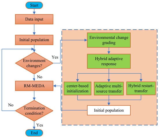
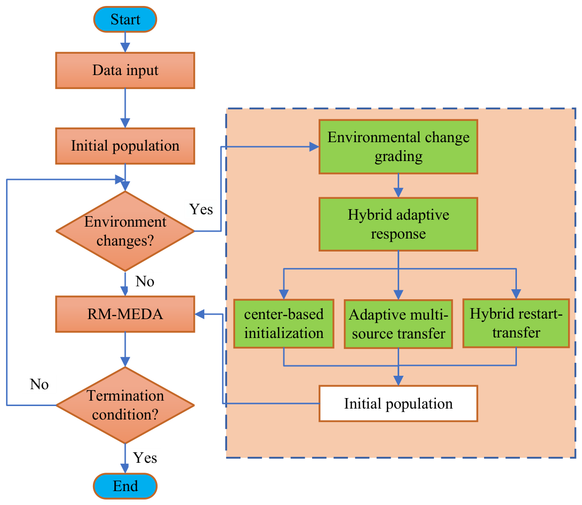
This section presents AMS-TL-RMMEDA, an adaptive multi-source transfer learning-based DMOEA, which uses RM-MEDA [26] as its static optimization backbone. Figure 1 depicts the overall procedure, while Algorithm 1 gives the pseudocode.

Algorithm 1 Framework of AMS-TL-RMMEDA.

Input:  Dynamic environment sequence $\{E_1,E_2,\dots ,E_{K_e}\}$ Output:  Pareto optimal sets of all environments   1: Randomly initialize the population $P^0$ (satisfying the constraints)   2: Run RM-MEDA for static optimization (with constraint handling) to obtain $P{S}_1$ and $PO{F}_1$   3: Store the historical knowledge: final PS + PS center + knee point set   4: while change detected do   5:    $t=t+1$;   6:    Compute the change intensity   7:    Select the response strategy according to the change intensity: small (below ${\theta }_{low}$): center-based initialization; medium (between ${\theta }_{low}$ and ${\theta }_{high}$): adaptive multi-source knowledge transfer; large (above ${\theta }_{high}$): hybrid strategy   8:    Generate the initial population $P_t^{init}$   9:    Perform constraint repair and feasibility-based evaluation on $P_t^{init}$ 10:    Run RM-MEDA for static optimization to obtain $P{S}_t$ and $PO{F}_t$ 11:    Verify knee point quality: filter out low-quality transferred solutions 12:    Update the historical knowledge base: store the final PSt, its center, and the knee point set 13: end while 14: return the Pareto optimal sets of all environments

Figure 1. Flowchart of the proposed AMS-TL-RMMEDA for the dynamic appliance scheduling problem.

3.1. Environmental Change Grading and Response Strategy Selection

In the setting of this paper, each environment corresponds to one scheduling day (HEMS) or one benchmark time window, so change instants are known a priori; the task after a change is to grade its intensity and select a response accordingly. The intensity is measured by the average objective displacement of the archived Pareto solutions ${\mathcal{P}}_{t-1}$ of the previous environment (up to $\min (50,N_{pop})$ solutions), re-evaluated in the new environment:

$${\delta }_t={\displaystyle \frac{1}{|{\mathcal{P}}_{t-1}|}}\sum _{{\mathbf{x}}_i\in {\mathcal{P}}_{t-1}}\parallel \mathbf{F}({\mathbf{x}}_i,t)-\mathbf{F}({\mathbf{x}}_i,t-1)\parallel .$$

(17)

To make the thresholds portable across problems of different magnitude, ${\delta }_t$ is normalized to ${\Delta }_t\in [0,1]$ by running min–max normalization, and the response is selected according to ${\Delta }_t$:

$${\Delta }_t={\displaystyle \frac{{\delta }_t-{\delta }_{min}}{{\delta }_{max}-{\delta }_{min}}}$$

(18)

where ${\delta }_{min}$ and ${\delta }_{max}$ are the running minimum and maximum of ${\delta }_t$ observed so far:

$${\mathrm{strategy}}_t=\left\{\begin{array}{cc}\mathrm{center}\text{-}\mathrm{based}\mathrm{initialization},\hfill & {\Delta }_t<{\theta }_{low}\hfill \\ \mathrm{multi}\text{-}\mathrm{source}\mathrm{transfer},\hfill & {\theta }_{low}\le {\Delta }_t<{\theta }_{high}\hfill \\ \mathrm{hybrid}\mathrm{strategy},\hfill & {\Delta }_t\ge {\theta }_{high}.\hfill \end{array}\right.$$

(19)

The thresholds ${\theta }_{low}=0.3$ and ${\theta }_{high}=0.7$ are dimensionless constants, and the three levels carry a clear physical meaning: ${\Delta }_t<0.3$ indicates a slight change (e.g., the POF moves only marginally between adjacent environments under gradual drift), which center-based initialization can track; $0.3\le {\Delta }_t<0.7$ indicates a marked change that calls for multi-source transfer of historical knowledge; and ${\Delta }_t\ge 0.7$ indicates an abrupt change, where random diversity must be injected to avoid negative transfer. Running min–max normalization presumes sufficient intensity variation across environments: it holds for the DF benchmark of Section 4 but degenerates under the HEMS drift patterns, where fixed absolute thresholds on ${\delta }_t$ are adopted instead (Section 5.2).

3.2. Adaptive Multi-Source Knowledge Transfer

3.2.1. Knowledge Extraction

Conventional transfer learning-based DMOEAs draw only on the most recent environments. In contrast, the proposed algorithm exploits every historical environment $E_j$, $j=1,\dots ,t-1$, and archives two kinds of knowledge for each:

• PS information: The final Pareto set $P{S}^{\left(j\right)}$ and its center ${\mathbf{c}}^{\left(j\right)}$ (the mean of the Pareto solutions), which together characterize the PS manifold.
• Knee point set: The knee points $\{{\mathbf{k}}_1^{\left(j\right)},\dots ,{\mathbf{k}}_{n_k}^{\left(j\right)}\}$ on the Pareto front of that environment.

3.2.2. Environment Similarity

Because the PS manifold of appliance scheduling varies periodically, the similarity between the current environment $E_t$ and each $E_j$ is quantified by the Hausdorff distance between their fronts. Two implementation aspects deserve note. First, the current POF is unknown before optimization, and is approximated by a probe population of 50 random solutions evaluated in the new environment. Second, the distance is computed in the objective space; the POF is the $(m-1)$-dimensional image of the PS manifold and carries equivalent manifold information, whereas the Hausdorff distance of a handful of points in the high-dimensional decision space carries little statistical meaning,

$$D_H(E_t,E_j)=\max \left(\underset{\mathbf{p}\in PO{F}_t}{\max }\underset{\mathbf{q}\in PO{F}_j}{\min }\parallel \mathbf{p}-\mathbf{q}\parallel ,\underset{\mathbf{q}\in PO{F}_j}{\max }\underset{\mathbf{p}\in PO{F}_t}{\min }\parallel \mathbf{p}-\mathbf{q}\parallel \right),$$

(20)

where $PO{F}_t$ collects the objective values of the probe population and $PO{F}_j$ the historical Pareto front. The similarity follows as

$$sim(E_t,E_j)=\exp \left(-\lambda ·D_H(E_t,E_j)\right),$$

(21)

with decay coefficient $\lambda$. Since $sim\in (0,1]$, larger values indicate more similar environments. Allocating weights directly from this front-level geometric similarity is computationally cheap and physically interpretable: in appliance scheduling, similar environments (e.g., the same periods on different days) have nearly coinciding Pareto fronts, which the Hausdorff distance captures well.

3.2.3. Adaptive Transfer Weights

The transfer weight of each historical environment follows from the similarities:

$${\omega }_j={\displaystyle \frac{sim(E_t,E_j)}{{\sum }_{l=1}^{t-1}sim(E_t,E_l)}}$$

(22)

so that more similar environments contribute more knowledge. When an environment differs greatly from the current one ($sim\to 0$), its weight approaches zero, which suppresses negative transfer. Rather than selecting only the most similar and the most recent environments as two explicit sources [20], the algorithm weights all historical environments continuously, allowing it to more fully exploit the available information.

3.2.4. Knee Point Selection in Three Objectives

In bi-objective problems, the knee point is the point of maximum curvature on the Pareto front curve [27]. For three or more objectives, KnEA [28] defines knee points as the solutions farthest from the hyperplane spanned by the extreme points in the normalized objective space. Since the POF of the present three-objective problem is a 2D surface, this definition is adopted as a practical proxy for the maximum normal curvature.

Let ${\tilde{\mathbf{f}}}_1$, ${\tilde{\mathbf{f}}}_2$, and ${\tilde{\mathbf{f}}}_3$ be the normalized extreme solutions minimizing $f_1$, $f_2$, and $f_3$, respectively, and let $\hat{\mathbf{n}}$ be the unit normal of the plane they span. The knee degree of a non-dominated solution ${\mathbf{f}}^{*}$ is its distance to this plane:

$$\kappa \left({\mathbf{f}}^{*}\right)=\left|{({\tilde{\mathbf{f}}}^{*}-{\tilde{\mathbf{f}}}_1)}^{\top }\hat{\mathbf{n}}\right|.$$

(23)

The $n_k$ solutions with the largest knee degrees are chosen iteratively, with a minimum separation mechanism that excludes the neighborhood (radius 0.05 in the normalized space) of each selected solution from subsequent rounds to prevent clustering. In the three-objective space, knee points lie near the “ridge” of the POF surface, where the marginal rate of substitution changes fastest, making them the most instructive candidates for user decisions.

Low-quality knee points can mislead the transfer, so a quality check based on the domination count is carried out as well. The transferred solutions are merged with the probe population evaluated in the new environment, and the domination count of every merged solution is computed; only transferred solutions for which the count falls within the best 30% of the merged set are retained. This filter keeps the transfers that genuinely help the current environment and further lowers the risk of negative transfer.

3.2.5. GFK-Based Manifold Transfer

For each historical environment $E_j$, the knee point set is transferred to the current environment through a GFK-based subspace alignment. The geodesic flow kernel [29] aligns source and target feature subspaces on the Grassmann manifold, and has been applied to manifold transfer in dynamic multi-objective optimization [13,30]; here a practical SVD-based variant [13] is used. Let ${\mathbf{P}}_j$ and ${\mathbf{P}}_t$ collect the leading d principal components of the knee point set of $E_j$ and of the probe population, respectively, and let $[\mathbf{U},\sim ,\mathbf{V}]=\mathrm{svd}\left({\mathbf{P}}_j^{\top }{\mathbf{P}}_t\right)$. The transfer matrix is ${\mathbf{G}}_j={\mathbf{P}}_j\mathbf{U}{\mathbf{V}}^{\top }{\mathbf{P}}_t^{\top }$ and the transferred solutions are

$${\tilde{\mathbf{k}}}_i^{\left(j\right)}=({\mathbf{k}}_i^{\left(j\right)}-{\mathit{\mu }}_j)·{\mathbf{G}}_j+{\mathit{\mu }}_t,$$

(24)

where ${\mathit{\mu }}_j$ and ${\mathit{\mu }}_t$ are the means of the source knee point set and the target probe population, respectively.

The transfers from all historical environments are then aggregated by proportional allocation. From each $E_j$, $n_j=\mathrm{round}({\omega }_j·n_{max})$ solutions are drawn and merged into

$${\mathbf{S}}^{transfer}=\bigcup _{j:{\omega }_j\ge 0.01}{\tilde{\mathbf{K}}}^{\left(j\right)},|{\tilde{\mathbf{K}}}^{\left(j\right)}|=\mathrm{round}\left({\omega }_j·n_{max}\right),$$

(25)

where ${\tilde{\mathbf{K}}}^{\left(j\right)}$ is the transferred knee set of $E_j$ and $n_{max}$ is the size of the transferred set. Environments with ${\omega }_j<0.01$ are skipped in order to avoid negative transfer, and any shortfall relative to $n_{max}$ is covered by elites from the most recent environment. In this way, similar environments contribute their high-quality information in full, while dissimilar ones are muted by low weights.

3.3. Hybrid Adaptive Response Framework

When a change occurs, the response is selected according to the change intensity (Equation (18)). Center-based initialization, multi-source transfer, and the hybrid restart–transfer strategy are integrated into a single framework that is tightly coupled with the transfer mechanism of Section 3.2.

When the change is small, the new PS is expected to stay close to the previous one. Following the idea of exploiting PS center information from past environments [31,32], the initial population combines 70% individuals sampled around the previous PS center (Gaussian sampling with a standard deviation of 10% of the variable range) with 30% elites inherited from the previous environment. This response is the cheapest, and remains sufficiently accurate under slight changes.

When the change is moderate, the adaptive multi-source transfer extracts and transfers knee points from all historical environments; its weighted aggregation (Equation (25)) integrates knowledge from multiple environments into a high-quality initial population.

When the change is drastic, there is a risk of transfer becoming misled; therefore, a hybrid strategy is adopted in which 30% non-dominated solutions of the current population are retained in order to preserve elite information, 30% multi-source transferred solutions exploit historical knowledge at a reduced share, and 40% randomly generated individuals inject diversity:

$$P_t^{init}=\left\{P_{elite}^{(30\%)}\right\}\cup \left\{S_{transfer}^{(30\%)}\right\}\cup \left\{P_{rand}^{(40\%)}\right\}.$$

(26)

This blend balances the exploitation of historical knowledge against population diversity under abrupt changes, thereby avoiding the failure of purely transfer-based responses in such regimes.

3.4. Constraint Handling

The model involves five constraints, which are handled as follows:

(1) Admissible-slot and PV accommodation constraints (Equations (9) and (13)): The admissible slot constraint is enforced at initialization and evaluation. Slots with $p{m}_i\left(\tau \right)=0$ (i.e., $\tau \notin {\mathcal{A}}_i$) are forced to $x_{i,\tau }=0$ and excluded from the search, while the PV accommodation constraint is satisfied by construction through $P_s^{grid}\left(\tau \right)=\max (0,·)$ and needs no extra treatment.

(2) Operation duration constraint (Equation (10)): Handled by a repair operator; if the total duration of an appliance falls below $T_i^{min}$, slots are added within its admissible set in descending order of preference, while if it exceeds $T_i^{max}$, surplus slots are removed in ascending order of preference.

(3) Continuous operation constraint (Equation (11)): After new solutions are sampled, interruptions of uninterruptible appliances are detected, then the longest continuous segment is retained and extended until $T_i^{req}$ is met.

(4) Power constraint (Equation (12)): Handled by the constrained domination (feasibility) rule [33] during environmental selection; each individual carries a violation degree $V={\sum }_{\tau =1}^T\max (0,P^{total}\left(\tau \right)-P^{max})$, with infeasible individuals ranked behind all feasible ones in ascending order of violation and feasible individuals compared by Pareto domination and pruned by density.

RM-MEDA operates in a continuous space, whereas $x_{i,\tau }$ is binary; therefore, all appliances share a unified $N\times T$ continuous encoding $\mathbf{y}\in {[0,1]}^{N\times T}$, binarized by the rule $x_{i,\tau }=1$ if and only if $y_{i,\tau }\ge 0.5$.

Encoding and repair for uninterruptible appliances: Although the encoding is unified, the repair operator collapses the effective search space of an uninterruptible appliance to its start time; only the longest continuous segment is kept and extended to a block of exactly $T_i^{req}$ slots, which is equivalent to searching the start time of a length-$T_i^{req}$ block and satisfies the continuous operation constraint (Equation (11)) by construction. The interruptible water heater retains the full 0–1 encoding, so its operation may be split into segments within ${\mathcal{A}}_i$ for greater scheduling flexibility.

4. Benchmark Experiments

4.1. Experiment Settings

The popular DF suite [34] serves as the test bed. It comprises DF1–DF9 with two objectives and DF10–DF14 with three objectives, allowing the tracking ability of the algorithms under different change types to be examined systematically. Four representative DMOEAs are chosen as baselines: D-NSGA-II [33], RI-ISDE+ [35], Tr-RM-MEDA [16], and HETD-RM-MEDA [12]. Table 2 summarizes the parameter settings. The modified inverse generational distance (MIGD) and modified hypervolume (MHV) are adopted to assess performance [17].

Table 2. Parameter settings.

Parameter Variables	Parameter Values	Parameter Variables	Parameter Values
Change intensity	$n_t=10$	Change frequency	${\tau }_t=10$
Number of clusters	$K=5$	Number of knee points	$n_k=10$
Decay coefficient	$\lambda =2.0$	Change intensity thresholds	${\theta }_{low}=0.3$, ${\theta }_{high}=0.7$
Population size	$N_{pop}=100$	Number of dynamic environments	$K_e=30$
Number of decision variables	$D=10$

The parameters in Table 2 follow established conventions. The change severity $n_t=10$, change frequency ${\tau }_t=10$, number of environments $K_e=30$, and number of decision variables $D=10$ follow the standard CEC 2018 DF configuration [34]. The population size $N_{pop}=100$ and per-environment iteration budget of 100 generations follow [33] and are identical for all compared algorithms. The number of clusters $K=5$ follows the original RM-MEDA [26]. The knee count $n_k=10$ amounts to about 10% of the population, which suffices to span the front ridge while keeping the subspace estimation stable. The decay coefficient $\lambda =2.0$ calibrates the exponential kernel so that the similarity decays noticeably over the range of Hausdorff distances encountered in practice, and the thresholds ${\theta }_{low}=0.3$ and ${\theta }_{high}=0.7$ divide the normalized intensity range $[0,1]$ evenly into small, medium, and large changes. All parameters of the baseline algorithms follow their original papers. Each algorithm is run 20 times independently on each test problem.

4.2. Comparison with Other DMOEAs

Table 3 and Table 4 report the MIGD and MHV values of all algorithms, where “+”, “−”, and “≈” respectively indicate that AMS-TL-RMMEDA performs better, worse, or comparably; boldface marks the best value per problem. The “+”, “−”, and “≈” symbols in Table 3 and Table 4 compare the mean values over these runs. Entries for which the means coincide at the reported precision are marked as comparable (≈). AMS-TL-RMMEDA attains 8 of the 14 best MIGD outcomes, against four for D-NSGA-II and one each for RI-ISDE+ and HETD-RM-MEDA; in addition, it surpasses Tr-RM-MEDA on 12 of the 14 problems in MIGD and on all 14 problems in MHV. The POF of DF4 is a symmetric curve, and its shape varies between convex and concave over time; on this problem, D-NSGA-II, RI-ISDE+, and HETD-RM-MEDA slightly outperform the proposed algorithm in terms of MIGD, while the proposed algorithm remains nearly optimal in terms of HV. Howerer, AMS-TL-RMMEDA exhibits inferior performance on DF6 and DF7, which can be attributed to the distinctive characteristics of these problems. The front of DF6 is disconnected with a time-varying number of segments, so transferred solutions may land on vanishing segments, and the front of DF7 degenerates over part of the timeline, which penalizes any history-driven initialization.

Table 3. MIGD results obtained by compared DMOEAs for DF problems.

Problems	D-NSGA-II	RI-ISDE+	Tr-RM-MEDA	HETD-RM-MEDA	AMS-TL-RMMEDA
DF1	0.0465  ± 0.0001 (−)	0.0466 ± 0.0001 (−)	0.0467 ± 0.0000 (≈)	0.0468 ± 0.0001 (+)	0.0467 ± 0.0001
DF2	0.0064 ± 0.0000 (+)	0.0064 ± 0.0000 (+)	0.0045 ± 0.0000 (+)	0.0044 ± 0.0000 (≈)	0.0044 ± 0.0000
DF3	0.1662 ± 0.0017 (+)	0.2159 ± 0.0078 (+)	0.2257 ± 0.0156 (+)	0.1959 ± 0.0116 (+)	0.1656 ± 0.0001
DF4	1.1361 ± 0.0004 (−)	1.1357 ± 0.0005 (−)	1.3591 ± 0.1024 (+)	1.1350 ± 0.0019 (−)	1.1379 ± 0.0004
DF5	0.9362 ± 0.0006 (−)	0.9404 ± 0.0048 (+)	0.9965 ± 0.0187 (+)	0.9445 ± 0.0001 (+)	0.9374 ± 0.0005
DF6	1.6738 ± 0.5890 (+)	1.7103 ± 0.5662 (+)	2.3747 ± 0.3149 (+)	0.5393 ± 0.0406 (−)	1.3826 ± 0.4781
DF7	1.9574 ± 0.0005 (−)	1.9574 ± 0.0007 (−)	2.1572 ± 0.0182 (−)	2.0763 ± 0.0403 (−)	2.1690 ± 0.1170
DF8	0.1671 ± 0.0046 (+)	0.2602 ± 0.0088 (+)	0.3327 ± 0.0373 (+)	0.2464 ± 0.0028 (+)	0.1666 ± 0.0031
DF9	1.2030 ± 0.0155 (−)	1.3282 ± 0.0142 (+)	1.5129 ± 0.0569 (+)	1.2925 ± 0.0140 (+)	1.2615 ± 0.0136
DF10	0.2170 ± 0.0061 (+)	0.2959 ± 0.0158 (+)	0.1993 ± 0.0040 (+)	0.1966 ± 0.0013 (+)	0.1812 ± 0.0004
DF11	0.6617 ± 0.0009 (+)	0.6739 ± 0.0010 (+)	0.6610 ± 0.0006 (+)	0.6600 ± 0.0013 (+)	0.6555 ± 0.0005
DF12	0.1154 ± 0.0046 (+)	0.2508 ± 0.0151 (+)	0.0878 ± 0.0000 (+)	0.0853 ± 0.0009 (+)	0.0777 ± 0.0011
DF13	1.0723 ± 0.0113 (+)	1.1422 ± 0.0194 (+)	1.0573 ± 0.0073 (+)	1.0530 ± 0.0083 (+)	0.9984 ± 0.0048
DF14	0.8316 ± 0.0318 (+)	0.9608 ± 0.0535 (+)	0.6947 ± 0.0064 (+)	0.6941 ± 0.0040 (+)	0.6604 ± 0.0016
+/≈/−	9/0/5	11/0/3	12/1/1	10/1/3	–

Table 4. MHV results obtained by compared DMOEAs for DF problems.

Problems	D-NSGA-II	RI-ISDE+	Tr-RM-MEDA	HETD-RM-MEDA	AMS-TL-RMMEDA
DF1	0.7323 ± 0.0001 (+)	0.7329 ± 0.0001 (+)	0.7352 ± 0.0001 (+)	0.7356 ± 0.0000 (+)	0.7358 ± 0.0000
DF2	0.9255 ± 0.0001 (+)	0.9256 ± 0.0001 (+)	0.9284 ± 0.0001 (+)	0.9285 ± 0.0001 (+)	0.9287 ± 0.0000
DF3	0.5019 ± 0.0024 (+)	0.4380 ± 0.0095 (+)	0.4766 ± 0.0081 (+)	0.4946 ± 0.0035 (+)	0.5065 ± 0.0002
DF4	0.6129  ± 0.0002 (−)	0.6129 ± 0.0001 (−)	0.5393 ± 0.0128 (+)	0.6092 ± 0.0005 (+)	0.6128 ± 0.0000
DF5	0.5716 ± 0.0001 (+)	0.5719 ± 0.0005 (+)	0.5726 ± 0.0009 (+)	0.5740 ± 0.0001 (+)	0.5745 ± 0.0001
DF6	0.6651 ± 0.0018 (−)	0.6587 ± 0.0113 (−)	0.3797 ± 0.0353 (+)	0.5933 ± 0.0088 (+)	0.6546 ± 0.0372
DF7	0.0182 ± 0.0009 (−)	0.0182 ± 0.0008 (−)	0.0068 ± 0.0011 (+)	0.0086 ± 0.0005 (−)	0.0073 ± 0.0033
DF8	0.8051 ± 0.0032 (−)	0.7321 ± 0.0084 (+)	0.7150 ± 0.0120 (+)	0.7590 ± 0.0010 (+)	0.8046 ± 0.0023
DF9	0.4071 ± 0.0047 (+)	0.3981 ± 0.0027 (+)	0.3788 ± 0.0108 (+)	0.4122 ± 0.0057 (+)	0.4206 ± 0.0015
DF10	0.9492 ± 0.0040 (+)	0.8328 ± 0.0091 (+)	0.9020 ± 0.0067 (+)	0.9106 ± 0.0012 (+)	0.9647 ± 0.0028
DF11	0.1104 ± 0.0032 (+)	0.1067 ± 0.0007 (+)	0.1165 ± 0.0006 (+)	0.1178 ± 0.0024 (+)	0.1236 ± 0.0011
DF12	0.9848 ± 0.0051 (+)	0.8935 ± 0.0023 (+)	1.0098 ± 0.0012 (+)	1.0125 ± 0.0009 (+)	1.0232 ± 0.0012
DF13	0.6315 ± 0.0044 (+)	0.6271 ± 0.0177 (+)	0.7022 ± 0.0007 (+)	0.7043 ± 0.0013 (+)	0.7106 ± 0.0019
DF14	0.4569 ± 0.0304 (+)	0.4507 ± 0.0200 (+)	0.5602 ± 0.0002 (+)	0.5616 ± 0.0003 (+)	0.5636 ± 0.0006
+/≈/−	10/0/4	11/0/3	14/0/0	13/0/1	–

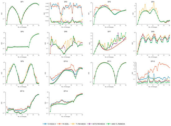
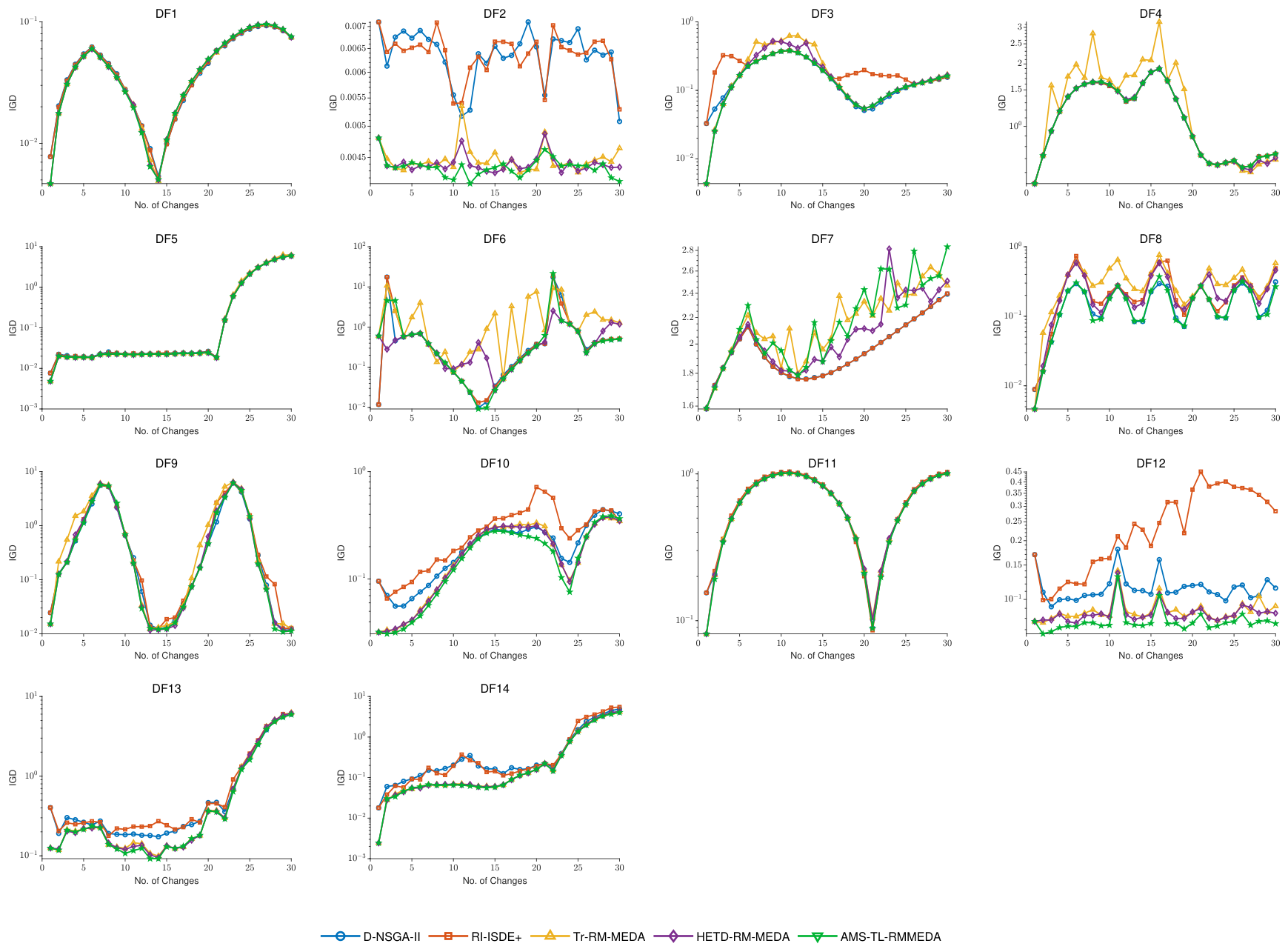
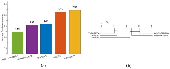
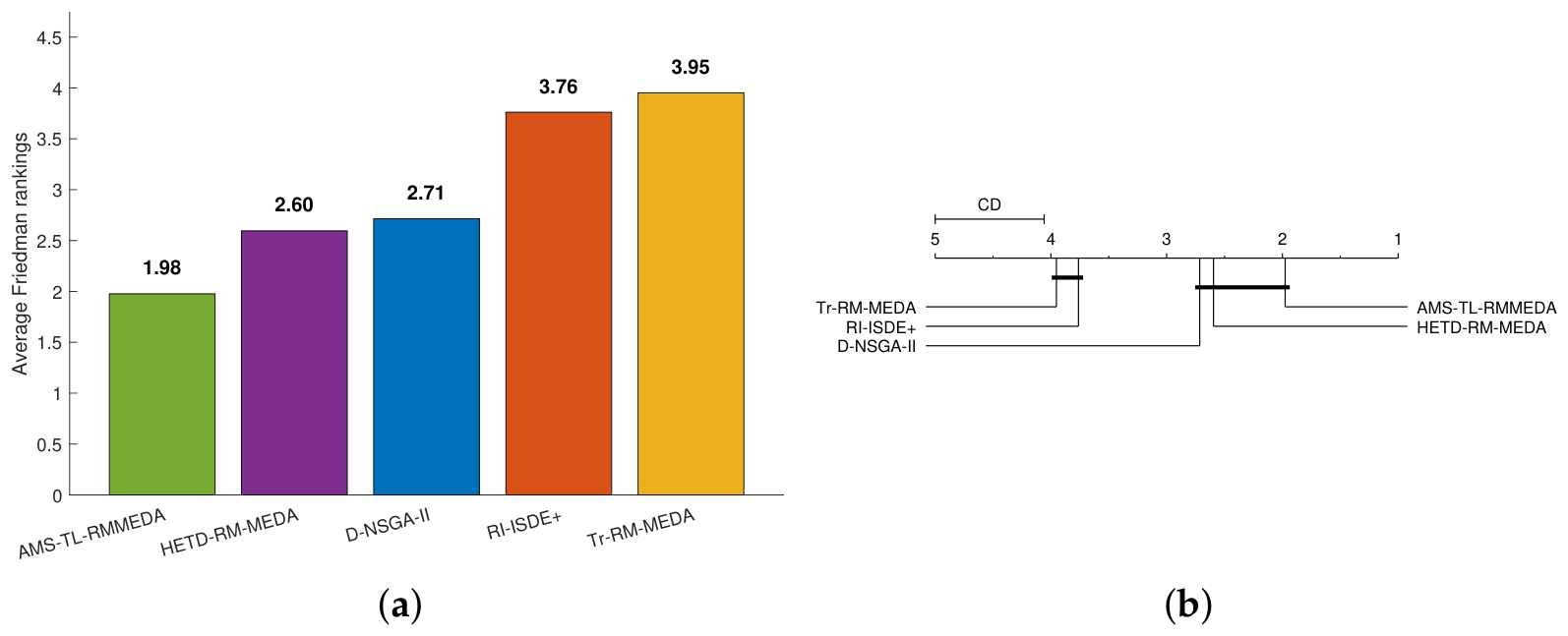
Figure 2 traces the average IGD values of the five algorithms over 30 environments on all 14 problems. The curves of AMS-TL-RMMEDA stay low in most environments, especially on the complex-front and three-objective problems such as DF3, DF8, and DF10–DF14. The Friedman test [36] further ranks the algorithms over all DF problems; Figure 3a shows the resulting average ranks. AMS-TL-RMMEDA attains the smallest rank (1.98), ahead of HETD-RM-MEDA (2.60), D-NSGA-II (2.71), RI-ISDE+ (3.76), and Tr-RM-MEDA (3.95). With the critical difference (CD) at the 0.05 level (Figure 3b), the top three algorithms are statistically indistinguishable, while AMS-TL-RMMEDA is significantly better than RI-ISDE+ and Tr-RM-MEDA.

Figure 2. IGD values obtained by five algorithms for different test functions.

Figure 3. Statistical tests of five compared algorithms for all test cases based on the MIGD values: (a) average ranks and (b) CD plot.

5. Results on Household Appliance Scheduling

The dynamic household appliance scheduling model is simulated here. The scheduling performance of AMS-TL-RMMEDA in comparison with representative DMOEAs is examined with eight controllable appliances, ten consecutive environments, and three weight drift patterns.

5.1. Simulation Scenario

The schedulable appliances include air conditioners, water heaters, electric vehicles (EVs), robot cleaners, rice cookers, washing machines, clothes dryers, and dishwashers [12]. Table 5 lists their parameters, including rated powers and preference levels. The water heater is interruptible and may operate in separate segments; the remaining devices must run continuously once started (“Uninterruptible = Yes” in the table) and are handled by the repair-based encoding of Section 3.4. The period is one day with $\Delta \tau =1$ h and 24 slots; the effect of the time resolution is examined in Section 5.3.4 against a 48-slot scheme at 0.5 h.

Table 5. Appliance parameters.

No.	Appliance	Rated Power (W)	Operation Duration (h)	Admissible Interval	Preferred Slots	Uninterruptible
1	Air conditioner	1500	6	[1,8] ∪ [13,24]	[1,8] ∪ [13,24]	Yes
2	Water heater	4000	2–4	[20,23]	[22,23]	No
3	Electric vehicle	5000	5	[1,7] ∪ [20,24]	[1,6] ∪ [23,24]	Yes
4	Robot cleaner	500	2	[10,19]	[13,19]	Yes
5	Rice cooker	1200	1	[2,7] ∪ {12,18}	{7,12,18}	Yes
6	Washing machine	600	2	[2,7] ∪ [20,24]	{7} ∪ [21,24]	Yes
7	Clothes dryer	1500	2	[1,6] ∪ [20,24]	{1} ∪ [22,24]	Yes
8	Dishwasher	2000	2	[2,8] ∪ [20,24]	{8} ∪ [23,24]	Yes

Note: For uninterruptible appliances, the operation duration is fixed to the required duration $T_i^{req}$ (equivalent to start-time encoding via repair); the water heater is interruptible, and its total operation duration varies within $[T_i^{min},T_i^{max}]=[2,4]$ h (required duration: 3 h).

We adopt the time-of-use tariffs for residential consumers in Shaanxi Province, China: 0.5483 CNY/kWh in peak periods (10:00–15:00 and 18:00–21:00), 0.4983 CNY/kWh in flat periods (7:00–10:00, 15:00–18:00, and 21:00–23:00), and 0.2983 CNY/kWh in valley periods (23:00–7:00 the next day) [15]. The grid carbon emission factors follow the officially released grid carbon footprint factors [37], assigned to the same peak/flat/valley partition as the TOU tariffs: 0.85 kgCO₂e/kWh in peak periods (coal-heavy generation), 0.60 kgCO₂e/kWh in flat periods, and 0.40 kgCO₂e/kWh in valley periods (wind- and nuclear-heavy). The CVaR confidence level $\alpha =0.95$ is the standard choice in risk management [25], and the $K_s=5$ equiprobable PV scenarios balance distribution fidelity against computational cost.

5.2. Dynamic Environment Settings

The dynamic environment consists of $K_e=10$ consecutive scheduling days. Each t ($t=1,\dots ,10$) is one complete 24-h cycle, and changes occur between days. The slot index $\tau$ ($\tau =1,\dots ,24$) and the day index t are orthogonal; every optimization decides the full 24 h of the current day (the decision matrix is always $N\times 24$), while the priority weights change across days. The tariffs, emission factors, and PV scenario tree are shared by all days.

The priority weights drift in one of three patterns:

• Gradual drift (Type I): $w_i^{\left(t\right)}=w_i^{\left(0\right)}+0.1(t-1)·\Delta w_i$, mimicking a slow, one-directional shift of user preferences.
• Random drift (Type II): $w_i^{\left(t\right)}=w_i^{\left(0\right)}+U(-0.3,0.3)·w_i^{\left(0\right)}$, mimicking irregular preference fluctuations.
• Realistic drift (Type III): A weekday-to-weekend switch in which the first five days follow the weekday pattern (low daytime priorities, high evening priorities) and the last five follow the weekend pattern (markedly higher daytime priorities), producing an abrupt weight jump on the sixth day (Saturday).

In the HEMS experiments, the grading of Equation (19) uses fixed absolute thresholds ${\theta }_{low}=0.002$ and ${\theta }_{high}=0.015$ on ${\delta }_t$. The running min–max normalization of Equation (18) degenerates under both the constant pattern (Type I) and the pulse-like pattern (Type III), with the normalization range shrinking toward zero and the normalized value turning unstable. The two absolute thresholds were fixed by inspecting the ${\delta }_t$ sequences produced by pilot runs of the three drift patterns: the gradual day-to-day changes of Type I stay mostly below 0.002, the weekday-to-weekend jump of Type III clearly exceeds 0.015, and moderate fluctuations fall in between. They are kept fixed across all experiments to avoid overfitting. The PV output follows the scenario tree with $K_s=5$ typical scenarios (sunny, cloudy, overcast, rainy, and transitional), each with probability $p_s=0.2$.

The reference fronts used by the IGD/MIGD and HV metrics are constructed as follows: for each drift type and each environment, RM-MEDA is run with a population of 200 for 150 generations from five random seeds, then the resulting fronts are merged and the dominated solutions are filtered out; to make the comparison fair, the reference runs use exactly the same weight sequence realization as the compared algorithms. Each compared algorithm is run 20 times independently in the HEMS study, with a population of 100 evolving for 50 generations per environment. The statistical significance is then assessed by the Friedman test with the critical-difference criterion.

5.3. Results Analysis

5.3.1. Comparison Before and After Scheduling

Before comparing the algorithms, the optimal scheduling value needs to be verified. The baseline starts each appliance in its most preferred slots (those with the highest preference levels) for the required duration, ignoring prices and emissions. The knee solutions of AMS-TL-RMMEDA under the three drift patterns are compared with this baseline, using the peak-to-average ratio (PAR) as a post hoc physical indicator [15]:

$$PAR={\displaystyle \frac{{\max }_{\tau }{P}^{total}\left(\tau \right)}{mea{n}_{\tau }{P}^{total}\left(\tau \right)}}$$

(27)

where $P^{total}\left(\tau \right)={\sum }_{i=1}^N{x}_{i,\tau }·P_i^{max}$ is the total household load at slot $\tau$.

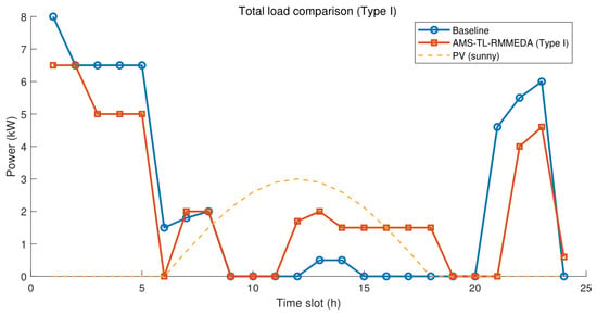
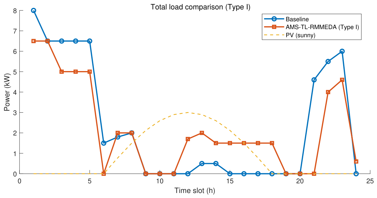
Figure 4 contrasts the load curves before and after scheduling, while Table 6 quantifies the comparison. Under Types I and II, optimization lowers the daily cost by about 16.6%, the emissions by about 17.3%, and the PAR by 12.5%; under Type III, the gains shrink because of the abrupt weekend jump. The dissatisfaction rises slightly, as part of the controllable load moves from preferred periods to cheap, low-carbon valley hours; this represents the expected trade-off among economy, comfort, and low-carbon goals.

Figure 4. Total household load curves before and after scheduling ($t=1$).

Table 6. Performance comparison before and after scheduling.

Metric	Baseline	Type I	Type II	Type III
Daily electricity cost (CNY)	20.10	16.75 (↓ 16.6%)	16.75 (↓16.6%)	19.15 (↓4.7%)
Daily carbon emissions (kgCO2e)	26.53	21.95 (↓17.3%)	21.95 (↓17.3%)	25.39 (↓4.3%)
User dissatisfaction	0.620	0.660 (↑6.5%)	0.680 (↑9.7%)	0.710 (↑14.5%)
PAR	3.40	2.98 (↓12.5%)	2.98 (↓12.5%)	3.40 (↓0.0%)

The residual fluctuation of the optimized curve in Figure 4 is structural: most controllable loads are uninterruptible, so their power enters and leaves the profile as rectangular blocks (the 6.5 kW night plateau is the overlap of the EV and dryer blocks). Even so, optimization lowers the peak demand from 8.0 kW to 6.5 kW (an 18.8% reduction), the standard deviation of the hourly load from 2.93 kW to 2.17 kW (25.9%), and the maximum hour-to-hour ramp from 6.0 kW to 5.0 kW, while the PAR drops by 12.5% (Table 6). The midday load blocks also coincide with the strongest PV output: across the five PV scenarios, the self-consumed share of the PV energy rises from 14.4–34.1% (baseline) to 49.4–66.6% after optimization.

5.3.2. Comparison with Other DMOEAs

Table 7 and Table 8 list the MIGD and MHV results under the three drift patterns, with the best value per column in bold. AMS-TL-RMMEDA delivers the best MIGD under all three patterns. Relative to HETD-RM-MEDA, its MIGD drops by 52.85% (Type I), 38.03% (Type II), and 51.12% (Type III). The gains stem from aggregating high-quality solutions of many historical environments, so the initial population covers a wider region of the PS manifold, an improvement in diversity and distribution on top of convergence. The results of KPMT-RM-MEDA [13] are included in Table 7 and Table 8. The proposed algorithm attains a lower MIGD under all three drift patterns, with reductions of 13.6% (Type I), 3.3% (Type II), and 4.0% (Type III) and a comparable MHV under Type II. The single-source knee transfer in KPMT-RM-MEDA preserves diversity well, whereas the advantage of AMS-TL-RMMEDA is concentrated in tracking convergence.

Table 7. MIGD results obtained by the compared algorithms.

Algorithm	MIGD (Type I)	MIGD (Type II)	MIGD (Type III)
D-NSGA-II	0.6327 ± 0.0323	0.6330 ± 0.0685	0.6689 ± 0.0796
RI-ISDE+	0.5516 ± 0.0817	0.7086 ± 0.0910	0.6822 ± 0.1317
Tr-RM-MEDA	0.2895 ± 0.0420	0.3126 ± 0.0529	0.3090 ± 0.0660
HETD-RM-MEDA	0.2195 ± 0.0222	0.2185 ± 0.0196	0.2445 ± 0.0253
KPMT-RM-MEDA	0.1198 ± 0.0265	0.1400 ± 0.0108	0.1245 ± 0.0161
AMS-TL-RMMEDA	0.1035 ± 0.0267	0.1354 ± 0.0313	0.1195 ± 0.0317

Table 8. MHV results obtained by the compared algorithms.

Algorithm	MHV (Type I)	MHV (Type II)	MHV (Type III)
D-NSGA-II	0.1054 ± 0.0014	0.1006 ± 0.0009	0.0970 ± 0.0009
RI-ISDE+	0.1056 ± 0.0004	0.0998 ± 0.0015	0.0969 ± 0.0003
Tr-RM-MEDA	0.1105 ± 0.0004	0.1058 ± 0.0005	0.1017 ± 0.0001
HETD-RM-MEDA	0.1109 ± 0.0003	0.1067 ± 0.0002	0.1017 ± 0.0002
KPMT-RM-MEDA	0.1133 ± 0.0002	0.1088 ± 0.0006	0.1039 ± 0.0005
AMS-TL-RMMEDA	0.1125 ± 0.0007	0.1088 ± 0.0006	0.1035 ± 0.0003

It is also worth quantifying how strongly the cost and carbon objectives conflict on this problem. Over the reference fronts of all ten Type-I environments, the Pearson correlation [38] between $f_1$ and $f_3$ is 0.938 on average; thus, the two objectives are strongly but not fully correlated: the residual conflict stems from the different peak/valley ratios of the tariff (0.5483/0.2983 = 1.84) and emission factor (0.85/0.40 = 2.13), so the cost-minimal and carbon-minimal schedules place the shiftable blocks in different periods. In this way, the carbon objective acts as a meaningful tie-breaker among near-equal-cost schedules and keeps the environmental footprint visible to the user, rather than acting as a fully independent axis.

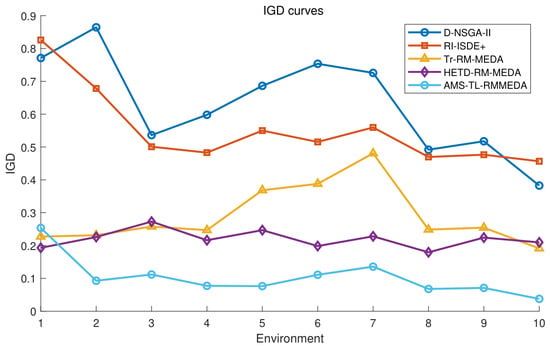
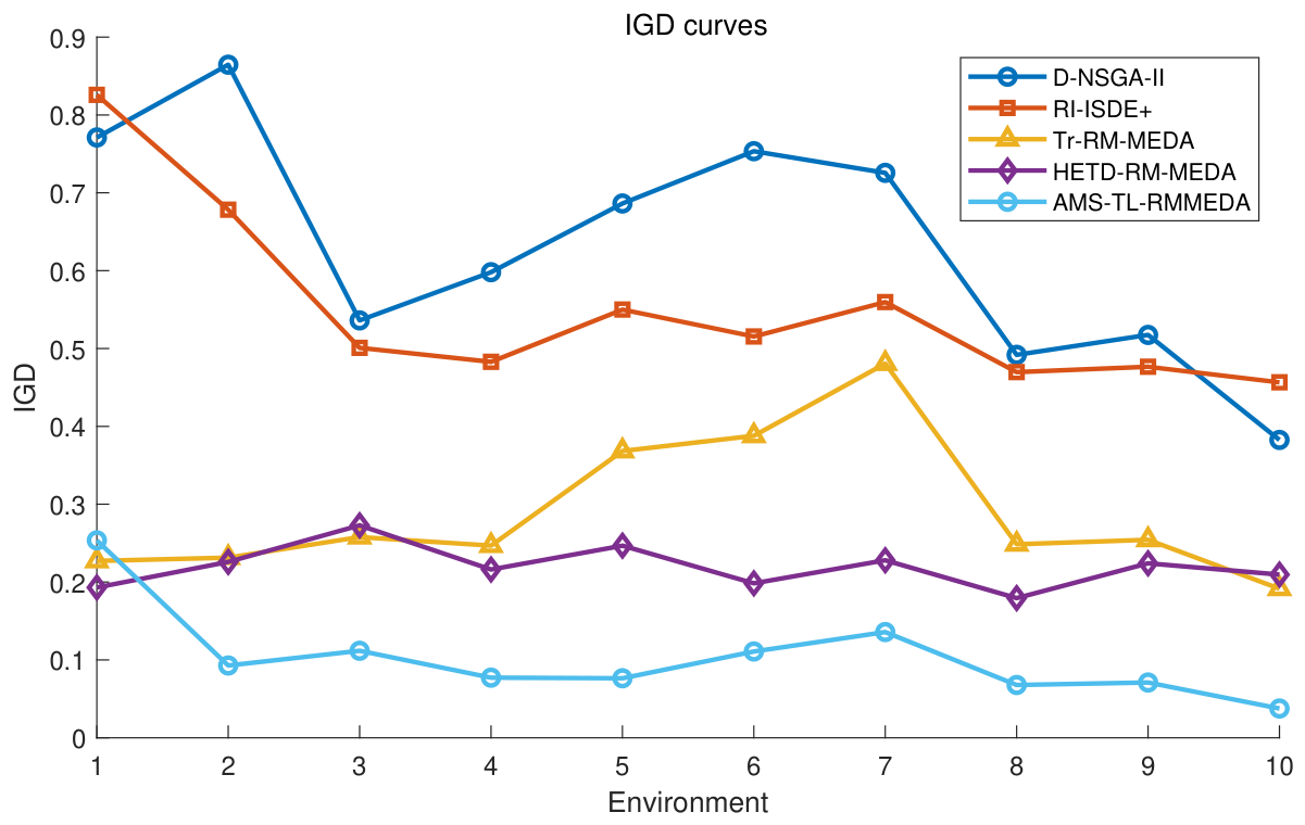
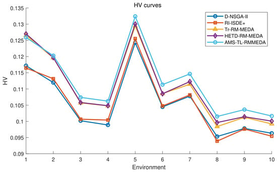
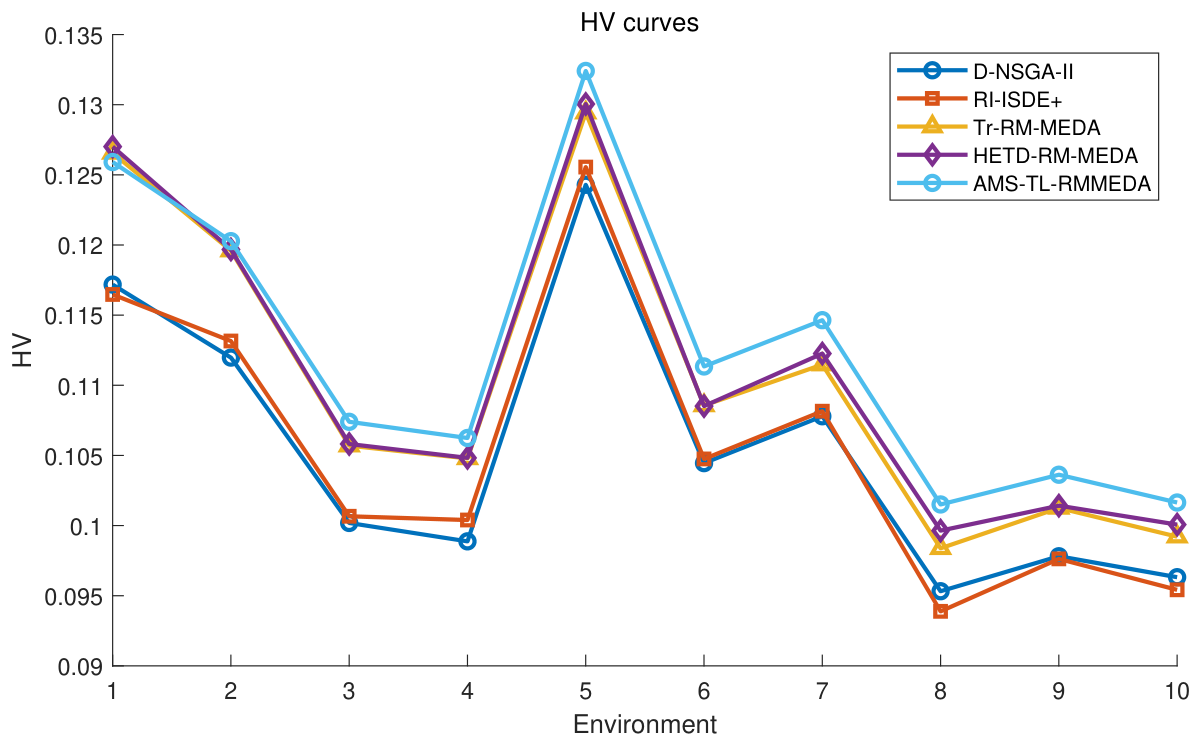
Figure 5 and Figure 6 visualize the per-environment IGD and HV under Type I over the ten environments. From these figures, it can be seen that AMS-TL-RMMEDA performs better than four compared algorithms in terms of both convergence and diversity; this is because as historical environments accumulate and the pool of transfer sources grows, adaptive weight aggregation is able to extract progressively more from them.

Figure 5. Per-environment IGD curves of the five algorithms under Type I drift.

Figure 6. Per-environment HV curves of the five algorithms under Type I drift.

A noticeable pattern in Figure 6 is that the five algorithms attain their Type I HV maxima simultaneously at Environment 5, while the inter-algorithm ranking is preserved in every environment. Since the HV of each environment is computed after normalizing the objectives by that environment’s own reference front, its absolute level reflects the volume dominated by the front in the normalized objective space; the preference weight configuration of Environment 5 happens to yield the front geometry with the largest such volume, so a well-converged population of any algorithm scores highest there.

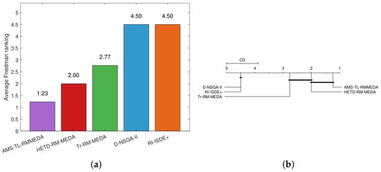
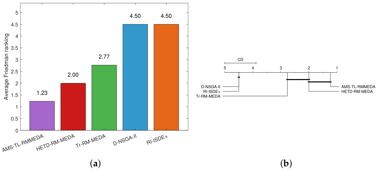
The average performance rankings of the compared algorithms are obtained using the Friedman test [36] based on their MIGD results. These rankings are presented in Figure 7a. The CD plot in Figure 7b shows the significance of the paired differences. AMS-TL-RMMEDA ranks first with an average score of 1.23, followed by HETD-RM-MEDA at 2.00. D-NSGA-II and RI-ISDE+ share the last score of 4.50, and both differ significantly from all transfer-based peers.

Figure 7. Statistical tests of five algorithms under three drift types based on the MIGD values: (a) average ranks and (b) CD plot.

5.3.3. Analysis of Household Appliance Scheduling Results

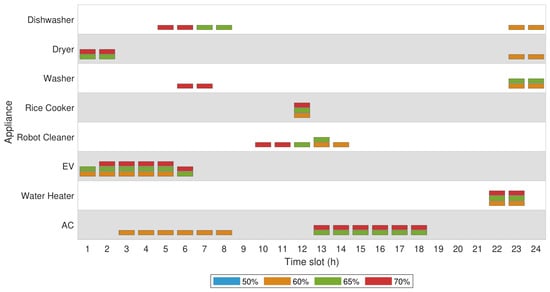
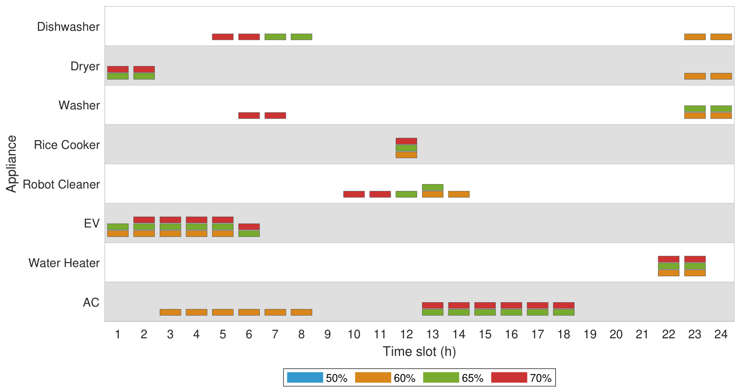
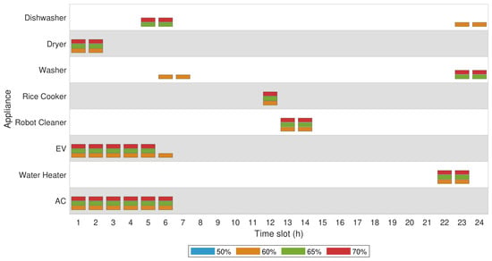
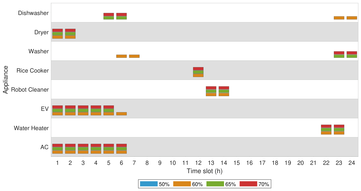
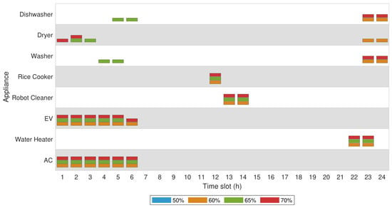
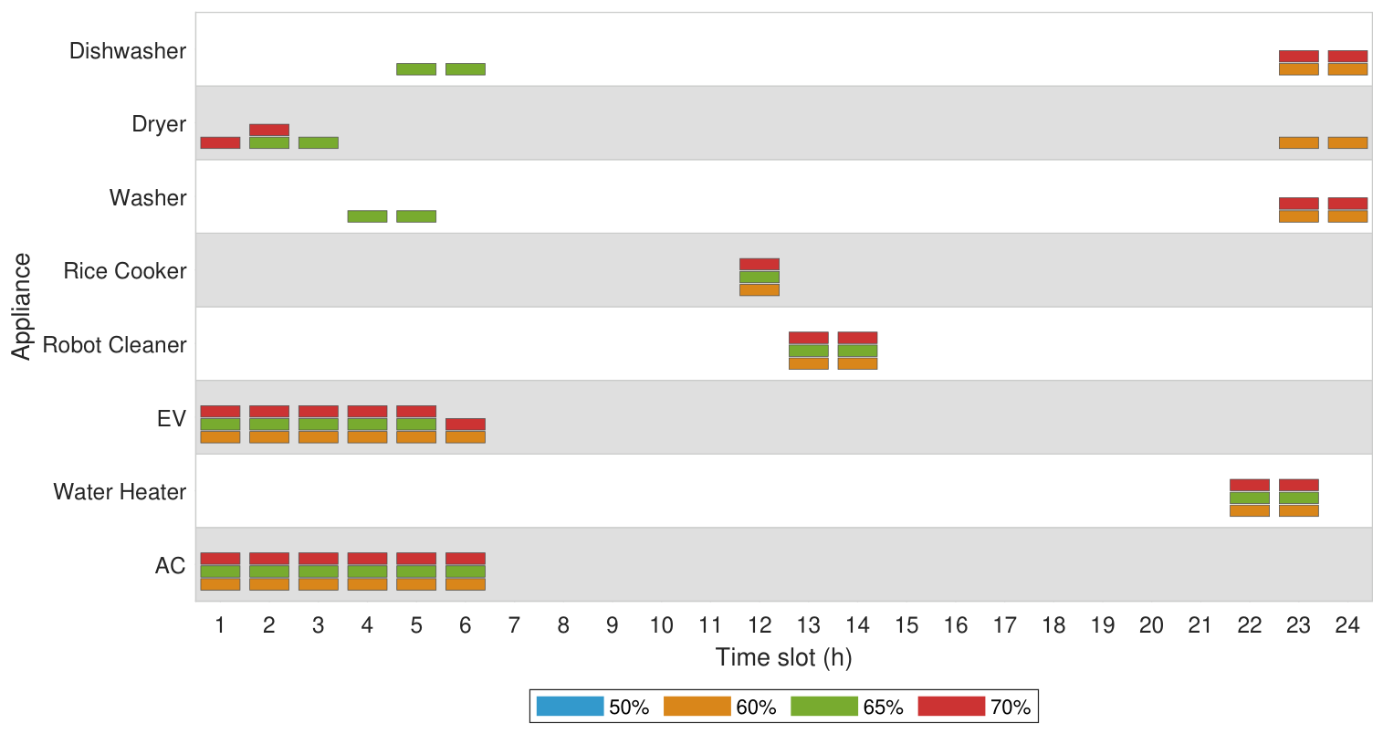
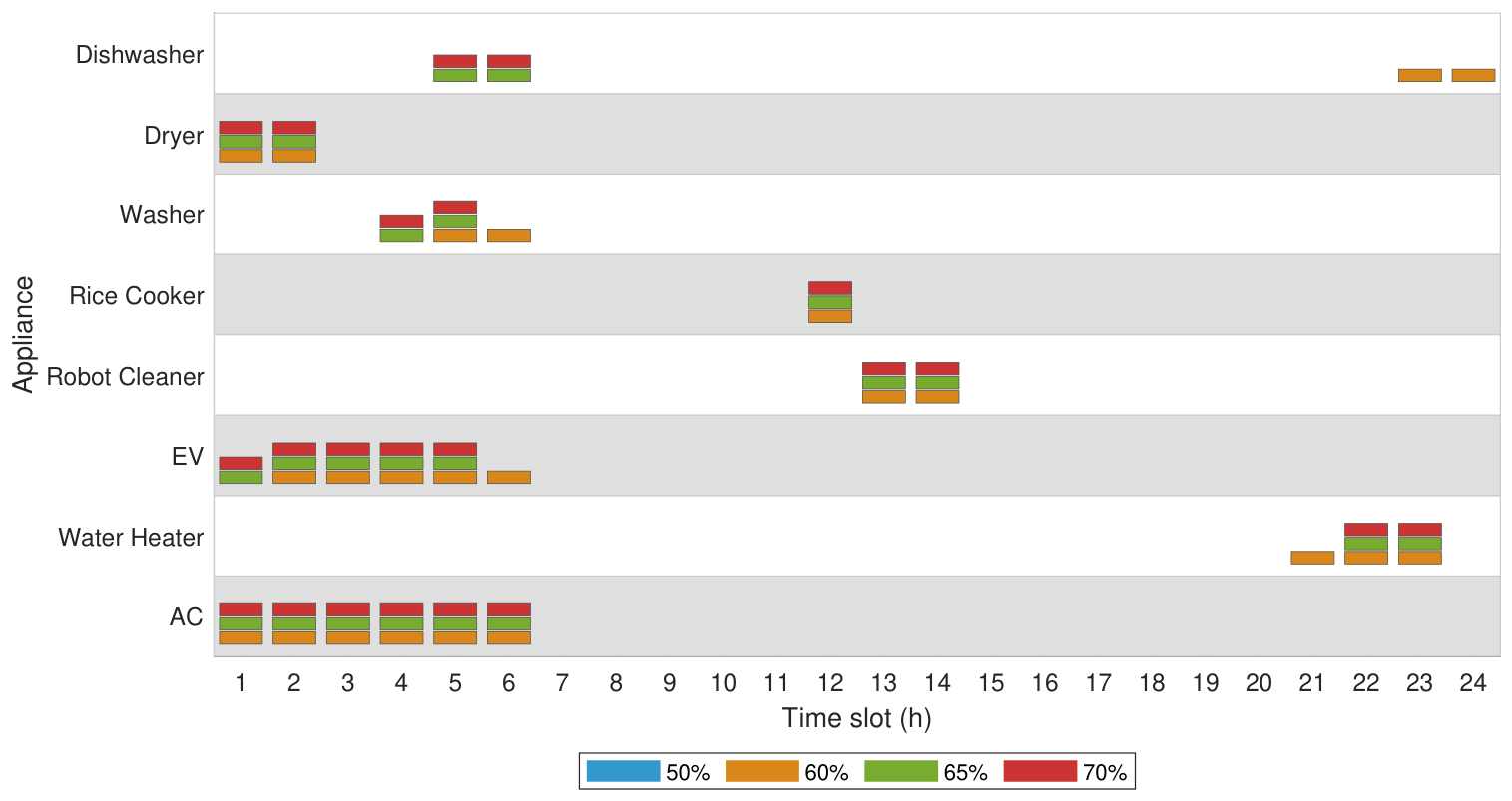
Figure 8, Figure 9, Figure 10 and Figure 11 present the optimal operation times of the appliances as stacked bar charts, obtained by AMS-TL-RMMEDA under Type I drift from $t=1$ to $t=4$ at dissatisfaction levels of 50%, 60%, 65%, and 70%. Each colored segment marks the scheduled operation of an appliance at a given time under a given level; for instance, a blue segment means that the appliance runs at that time under the 50% level.

Figure 8. On–off states of appliances with different user dissatisfactions at $t=1$.

Figure 9. On–off states of appliances with different user dissatisfactions at $t=2$.

Figure 10. On–off states of appliances with different user dissatisfactions at $t=3$.

Figure 11. On–off states of appliances with different user dissatisfactions at $t=4$.

Because the problem has three objectives, fixing the dissatisfaction level still leaves many Pareto-optimal solutions. A representative schedule is picked as follows: for each level, the solutions in which $f_2$ approximates that level (within 5%) form the two-dimensional sub-front of cost $f_1$ and emissions $f_3$; on this sub-front, the knee point, that is, the solution farthest from the line joining the two extreme points, is chosen as the best cost–carbon compromise. If the sub-front degenerates to a single solution, then it is taken directly; if no knee exists, then the solution with the smallest $f_1$ is taken.

The figures show that higher dissatisfaction levels shift more load into valley periods, cutting cost and emissions at the price of comfort. This is the trade-off along the three-objective front; across environments, the drifting weights alter the schedule at any fixed level, reflecting the dynamic nature of the problem.

5.3.4. Sensitivity Analysis

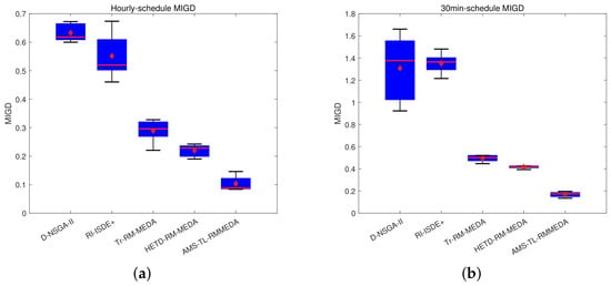
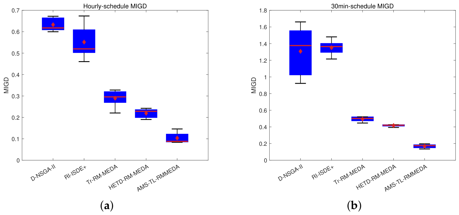
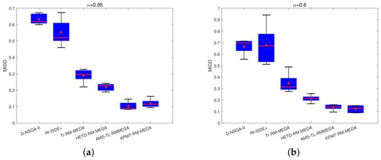
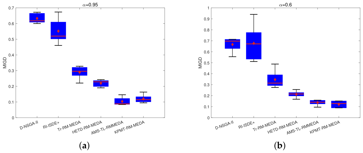
(A) Time Resolution. To probe robustness to the time resolution, the slot length is reduced from 1 h (24 slots) to 0.5 h (48 slots) under Type I drift. Figure 12 shows the resulting MIGD distributions as box plots. The ranking of the algorithms is identical under both resolutions, so the conclusions are insensitive to the resolution. Quantitatively, halving the slot length doubles the decision dimension from $8\times 24=192$ to $8\times 48=384$ and degrades every algorithm’s MIGD, but by very different margins; the mean MIGD of D-NSGA-II rises from 0.6327 to 1.3076 and that of RI-ISDE+ from 0.5516 to 1.3517, whereas AMS-TL-RMMEDA increases only from 0.1035 to 0.1687. Accordingly, its lead over HETD-RM-MEDA widens from 52.9% to 59.5%, indicating that multi-source transfer pays off even more in the higher-dimensional search space.

Figure 12. Statistical tests of five compared algorithms based on the MIGD values: (a) 24 time slots and (b) 48 time slots.

(B) Risk Parameter. As noted in Section 2.5.2, the CVaR degenerates to the worst-scenario cost at the adopted granularity ($K_s=5$, $\alpha =0.95$). To analyze the effect of risk parameter on the performance, the experiment is taken at $(1-\alpha )K_s=2$ ($\alpha =0.6$, tail = the two worst scenarios), with the reference fronts regenerated and the identical protocol. Figure 13 compares the resulting MIGD distributions with those of the main experiments under Type I drift. It can be seen that AMS-TL-RMMEDA remains better than D-NSGA-II, RI-ISDE+, Tr-RM-MEDA, and HETD-RM-MEDA under every drift pattern and both metrics; relative to KPMT-RM-MEDA, it is slightly outperformed in MIGD at this parameterization under Type I and II, suggesting that the multi-source transfer advantage is more pronounced under the more conservative risk regime.

Figure 13. MIGD distributions of the six algorithms at CVaR confidence levels (a) $\alpha =0.95$ and (b) $\alpha =0.6$ under Type I drift.

5.3.5. Comparison with AI-Based Scheduling Approaches

Model-free reinforcement learning (RL) is a strong alternative for HEMS scheduling. It learns dispatch policies by interacting with the household environment, requires no explicit appliance model, and adapts online to stochastic prices and PV output, as in adaptive RL [39], federated RL [40], and surrogate-assisted evolutionary–RL hybrids [41]. RL optimizes a scalarized reward, so the preference weights must be fixed in advance and the agent needs to be retrained once they drift; in comparison, AMS-TL-RMMEDA returns the whole Pareto front and its knee points in every environment, exposing the cost–comfort–carbon trade-off as preferences evolve.

5.3.6. Impacts on the Power Grid

Although a single household is optimized, the schedules carry grid-side implications. For peak load reduction, the knee solutions cut the household peak demand by 18.8% (from 8.0 kW to 6.5 kW) and the PAR by 12.5%; replicated across many households, this relieves distribution transformer stress and defers capacity reinforcement investment. For load shifting, the controllable load moves into the valley window and the midday PV-rich hours, which flattens the net load curve, raises PV self-consumption, and supports absorption of wind and nuclear generation. In terms of grid stability and energy efficiency, the PAR decreases from 3.40 to 2.98 and the hourly load variance decreases by 25.9%, so the schedules flatten out instead of concentrating the net load. From the perspective of renewable integration and decarbonization, the peak-period emission factor (0.85 kgCO₂e/kWh) is more than double that of the valley (0.40); this means that the 17.3% emission reduction is concentrated in the dirtiest periods, thereby amplifying the systemic decarbonization effect of demand response.

5.3.7. Limitations

Several limitations delimit the validity of this study. First, we use the preference drift alone to carry the dynamics; the tariffs, emission factors, and PV scenario tree are all shared across environments, so price- and weather-driven non-stationarity is not exercised. Second, the scenario dispersion shifts the schedules only mildly, since no storage is modeled; adding a battery or vehicle-to-grid operation would let PV uncertainty shape the decisions much more strongly. Third, only per-appliance constraints are modeled; sequencing dependencies among appliances, power ramp limits, and battery/EV vehicle-to-grid operation are not included.

6. Conclusions

This paper formulates a dynamic three-objective model for household appliance scheduling that simultaneously minimizes electricity cost, user dissatisfaction, and carbon emissions. We developed AMS-TL-RMMEDA, a DMOEA built on adaptive multi-source transfer learning. Environmental uncertainty is handled by a scenario tree that characterizes the variability of PV output, and the conditional value-at-risk criterion converts the stochastic electricity cost into a deterministic equivalent. The proposed AMS-TL-RMMEDA allocates transfer weights according to Hausdorff-based similarities and switches the change response adaptively among center-based initialization, multi-source knowledge transfer, and a hybrid restart–transfer strategy according to the quantified change intensity. On the DF1–DF14 benchmark suite, AMS-TL-RMMEDA attains the best MIGD on 8 of 14 problems, with the smallest average Friedman rank. In scheduling simulations with eight appliances and three drift patterns, it consistently outperforms compared algorithms on MIGD values, producing schedules that lower both electricity cost and carbon emissions while reducing the peak-to-average ratio.

Several directions remain open for future work. Deep reinforcement learning could be integrated for load forecasting and user behavior modeling, enabling data-driven prediction of the dynamic environment parameters. Richer constraints such as appliance sequencing and power ramp limits could also be incorporated to bring the model closer to practical deployment. A flatter household load profile could be pursued through an explicit PAR or ramp-rate constraint, or alternatively through a finer scheduling resolution, though at the price of squeezing the cost and carbon margins.

References

- Yahia, Z.; Pradhan, A. Multi-objective optimization of household appliance scheduling problem considering consumer preference and peak load reduction. Sustain. Cities Soc. 2020, 55, 102058. [Google Scholar] [CrossRef] [Scilit]
- Varghese, B.K.; Das, N.; Ray, B.; Mazid, A.M.; Jahan, I.; Nur-E-Alam, M. Optimisation algorithms used in home energy management systems: A review. Energy Build. 2025, 347, 116338. [Google Scholar] [CrossRef] [Scilit]
- Xiong, B.; Wei, F.; Wang, Y.; Xia, K.; Su, F.; Fang, Y. Hybrid robust-stochastic optimal scheduling for multi-objective home energy management system with uncertainties. Energy 2024, 290, 130047. [Google Scholar] [CrossRef] [Scilit]
- Liu, S.; Xie, Z.; Hu, Z.; Zhang, K.; Gao, W.; Liu, X. Ultra-short-term forecasting-based optimization for proactive home energy management. Energies 2025, 18, 3936. [Google Scholar] [CrossRef] [Scilit]
- Fiorotti, R.; Fardin, J.F.; Rocha, H.R.O.; Rua, D.; Lopes, J.A.P. Day-ahead optimal scheduling considering thermal and electrical energy management in smart homes with photovoltaic-thermal systems. Appl. Energy 2024, 374, 124070. [Google Scholar] [CrossRef] [Scilit]
- United Nations. Transforming Our World: The 2030 Agenda for Sustainable Development; Resolution A/RES/70/1; UN General Assembly: New York, NY, USA, 2015.
- Javadi, M.S.; Esmaeel Nezhad, A.; Nardelli, P.H.J.; Gough, M.; Lotfi, M.; Santos, S. Self-scheduling model for home energy management systems considering the end-users discomfort index within price-based demand response programs. Sustain. Cities Soc. 2021, 68, 102792. [Google Scholar] [CrossRef] [Scilit]
- El-Afifi, M.I.; Sedhom, B.E.; Eladl, A.A.; Elgamal, M.; Siano, P. Demand side management strategy for smart building using multi-objective hybrid optimization technique. Results Eng. 2024, 22, 102265. [Google Scholar] [CrossRef] [Scilit]
- Qayyum, N.; Jamil, U.; Mahmood, A. Optimizing energy cost in the residential sector through home energy management systems in a smart grid environment. Energy Explor. Exploit. 2025, 43, 1647–1664. [Google Scholar] [CrossRef] [Scilit]
- Wang, X.; Mao, X.; Khodaei, H. A multi-objective home energy management system based on Internet of Things and optimization algorithms. J. Build. Eng. 2021, 33, 101603. [Google Scholar] [CrossRef] [Scilit]
- Jiang, S.; Zou, J.; Yang, S.; Yao, X. Evolutionary Dynamic Multi-objective Optimisation: A Survey. ACM Comput. Surv. 2022, 55, 1–47. [Google Scholar] [CrossRef] [Scilit]
- Zhang, X.; Jin, Y.; Wu, P.; Liu, Q. Dynamic multi-objective home appliance scheduling using transfer learning based evolutionary algorithm. In Proceedings of the 2024 6th International Conference on Data-driven Optimization of Complex Systems (DOCS); IEEE: New York, NY, USA, 2024; pp. 438–444. [Google Scholar] [CrossRef] [Scilit]
- Zhang, X. Dynamic knowledge guided transfer optimal scheduling for home energy management system considering user preference. Sustainability 2025, 17, 10844. [Google Scholar] [CrossRef] [Scilit]
- Maurya, V.K.; Nanda, S.J. Time-varying multi-objective smart home appliances scheduling using fuzzy adaptive dynamic SPEA2 algorithm. Eng. Appl. Artif. Intell. 2023, 121, 105944. [Google Scholar] [CrossRef] [Scilit]
- He, X.; Yan, X. Optimal scheduling strategy of household electrical equipment based on scenario dynamic modeling. Energy Build. 2024, 324, 114945. [Google Scholar] [CrossRef] [Scilit]
- Jiang, M.; Huang, Z.; Qiu, L.; Huang, W.; Yen, G.G. Transfer learning-based dynamic multiobjective optimization algorithms. IEEE Trans. Evol. Comput. 2018, 22, 501–514. [Google Scholar] [CrossRef] [Scilit]
- Jiang, M.; Wang, Z.; Hong, H.; Yen, G.G. Knee point-based imbalanced transfer learning for dynamic multiobjective optimization. IEEE Trans. Evol. Comput. 2021, 25, 117–129. [Google Scholar] [CrossRef] [Scilit]
- Lin, Q.; Ye, Y.; Ma, L.; Jiang, M.; Tan, K.C. Dynamic multiobjective evolutionary optimization via knowledge transfer and maintenance. IEEE Trans. Syst. Man Cybern. Syst. 2024, 54, 936–949. [Google Scholar] [CrossRef] [Scilit]
- Ye, Y.; Lin, Q.; Ma, L.; Wong, K.C. Multiple source transfer learning for dynamic multiobjective optimization. Inf. Sci. 2022, 607, 739–757. [Google Scholar] [CrossRef] [Scilit]
- Song, W.; Liu, Z.; Yu, J.; Sun, X.; Jin, Y.; Lai, K.W. Multisource and hidden source-based knowledge transfer for solving dynamic multiobjective optimization problems. IEEE Trans. Evol. Comput. 2025, 29, 1546–1560. [Google Scholar] [CrossRef] [Scilit]
- Zhao, S.; Zhang, T.; Chen, M.; Zhang, L. Twin-population multiple knowledge-guided transfer prediction framework for evolutionary dynamic multi-objective optimization. Appl. Soft Comput. 2025, 175, 113113. [Google Scholar] [CrossRef] [Scilit]
- Wang, Z.; Xue, L.; Guo, Y.; Han, M.; Liang, S. Solving dynamic multi-objective optimization problems via quantifying intensity of environment changes and ensemble learning-based prediction strategies. Appl. Soft Comput. 2024, 154, 111317. [Google Scholar] [CrossRef] [Scilit]
- Haj Issa, H.; Abedini, M.; Hamzeh, M.; Anvari-Moghaddam, A. Day-ahead multi-criteria energy management of a smart home under different electrical rationing scenarios. Renew. Energy Focus 2024, 51, 100647. [Google Scholar] [CrossRef] [Scilit]
- Luthander, R.; Widén, J.; Nilsson, D.; Palm, J. Photovoltaic self-consumption in buildings: A review. Appl. Energy 2015, 142, 80–94. [Google Scholar] [CrossRef] [Scilit]
- Rockafellar, R.T.; Uryasev, S. Optimization of conditional value-at-risk. J. Risk 2000, 2, 21–41. [Google Scholar] [CrossRef] [Scilit]
- Zhang, Q.; Zhou, A.; Jin, Y. RM-MEDA: A regularity model-based multiobjective estimation of distribution algorithm. IEEE Trans. Evol. Comput. 2008, 12, 41–63. [Google Scholar] [CrossRef] [Scilit]
- Chen, G.; Guo, Y.; Yang, X.; Ma, T.; Yang, S.; Yuan, L. Dynamic multiobjective evolutionary algorithm based on a knee point driven Gaussian model. Expert Syst. Appl. 2026, 297, 129325. [Google Scholar] [CrossRef] [Scilit]
- Zhang, X.; Tian, Y.; Jin, Y. A knee point-driven evolutionary algorithm for many-objective optimization. IEEE Trans. Evol. Comput. 2015, 19, 558–570. [Google Scholar] [CrossRef] [Scilit]
- Gong, B.; Shi, Y.; Sha, F.; Grauman, K. Geodesic flow kernel for unsupervised domain adaptation. In Proceedings of the 2012 IEEE Conference on Computer Vision and Pattern Recognition (CVPR 2012), Providence, RI, USA, 16–21 June 2012; IEEE: New York, NY, USA, 2012; pp. 2066–2073. [Google Scholar] [CrossRef] [Scilit]
- Zhang, X.; Yu, G.; Jin, Y.; Qian, F. An adaptive Gaussian process based manifold transfer learning to expensive dynamic multi-objective optimization. Neurocomputing 2023, 538, 126212. [Google Scholar] [CrossRef] [Scilit]
- Zhou, A.; Jin, Y.; Zhang, Q. A population prediction strategy for evolutionary dynamic multiobjective optimization. IEEE Trans. Cybern. 2014, 44, 40–53. [Google Scholar] [CrossRef] [Scilit] [PubMed]
- Hatzakis, I.; Wallace, D. Dynamic multi-objective optimization with evolutionary algorithms: A forward-looking approach. In Proceedings of the 8th Annual Conference on Genetic and Evolutionary Computation (GECCO 2006), New York, NY, USA, 8–12 July 2006; ACM: New York, NY, USA, 2006; pp. 1201–1208. [Google Scholar] [CrossRef] [Scilit]
- Deb, K.; Rao, N.U.B.; Karthik, S. Dynamic multi-objective optimization and decision-making using modified NSGA-II: A case study on hydro-thermal power scheduling. In Proceedings of the Evolutionary Multi-Criterion Optimization (EMO 2007); Springer: Berlin/Heidelberg, Germany, 2007; Volume 4403, pp. 803–817. [Google Scholar] [CrossRef] [Scilit]
- Jiang, S.; Yang, S.; Yao, X.; Tan, K.C.; Kaiser, M.; Krasnogor, N. Benchmark problems for CEC 2018 competition on dynamic multiobjective optimisation. In Technical Report, CEC 2018 Competition on Dynamic Multiobjective Optimisation; IEEE: New York, NY, USA, 2018; Available online: https://www.tech.dmu.ac.uk/~syang/TF-ECiDUE/TR-CEC2018-DMOP-Competition.pdf#1#2#1 (accessed on 1 August 2026).
- Pamulapati, T.; Mallipeddi, R.; Lee, M. Multi-objective home appliance scheduling with implicit and interactive user satisfaction modelling. Appl. Energy 2020, 267, 114690. [Google Scholar] [CrossRef] [Scilit]
- Carrasco, J.; García, S.; Rueda, M.; Das, S.; Herrera, F. Recent trends in the use of statistical tests for comparing swarm and evolutionary computing algorithms: Practical guidelines and a critical review. Swarm Evol. Comput. 2020, 54, 100665. [Google Scholar] [CrossRef] [Scilit]
- Ministry of Ecology and Environment of the People’s Republic of China; National Bureau of Statistics of China; National Energy Administration of China. Announcement on the Release of the 2024 Electricity Carbon Footprint Factors (Announcement No. 19 of 2025). 2025. Available online: https://www.ccn.ac.cn/carbon-market/cf/7646.html (accessed on 1 August 2026).
- Pearson, K. Mathematical contributions to the theory of evolution. III. Regression, heredity, and panmixia. Philos. Trans. R. Soc. London. Ser. A 1896, 187, 253–318. [Google Scholar] [CrossRef] [Scilit]
- Saroha, P.; Singh, G.; Lilhore, U.K.; Simaiya, S.; Khan, M.; Alroobaea, R.; Alsafyani, M.; Alsufyani, H. Dynamic appliance scheduling and energy management in smart homes using adaptive reinforcement learning techniques. Sci. Rep. 2025, 15, 24594. [Google Scholar] [CrossRef] [Scilit] [PubMed]
- Sumayli, M.; Anubi, O.M. Federated reinforcement learning for peak demand mitigation in residential energy systems with dynamic comfort preferences. IEEE Access 2026, 14, 8174–8187. [Google Scholar] [CrossRef] [Scilit]
- Dhruva, J.J.; Silvestri, S. Surrogate-assisted adaptive evolutionary algorithm for efficient HVAC control in home energy management systems. IEEE Access 2026, 14, 56010–56025. [Google Scholar] [CrossRef] [Scilit]
Disclaimer/Publisher’s Note: The statements, opinions and data contained in all publications are solely those of the individual author(s) and contributor(s) and not of MDPI and/or the editor(s). MDPI and/or the editor(s) disclaim responsibility for any injury to people or property resulting from any ideas, methods, instructions or products referred to in the content. |
© 2026 by the authors. Licensee MDPI, Basel, Switzerland. This article is an open access article distributed under the terms and conditions of the Creative Commons Attribution (CC BY) license.