


Abstract
Under rapid urbanization, fragmentation and declining connectivity of wetland landscapes may be accompanied by changes in ecosystem service (ES) supply and the balance among services. However, nonlinear associations between wetland landscape patterns and wetland ecosystem services (WESs), including candidate turning-point ranges, remain insufficiently understood. Taking Wuhan, China, as the study area, we quantified spatiotemporal changes in wetland landscape patterns and four core WESs—water yield, water purification, soil conservation, and habitat quality—from 2000 to 2020. We constructed an ecosystem service composite benefit index (ESS), an overall trade-off index (EST), and a synergistic benefit index (ESB), and used XGBoost and SHAP to identify nonlinear associations of landscape pattern metrics with WESs and ESB in 2020. The results showed that (1) Wuhan’s total wetland area decreased from 2000 to 2020, landscape fragmentation intensified, aggregation and connectivity declined, and multiple WESs showed downward trends in and around built-up areas; (2) the five landscape pattern metrics had marked nonlinear associations with WESs and ESB, with the mean shape index (SHAPE), aggregation index (AI), and largest patch index (LPI) contributing strongly to the models; and (3) the SHAP curves showed relatively stable ESB turning points near SHAPE 1.40 and AI 96%, while the central LPI crossing was near 61%. These values can serve as reference thresholds for wetland planning and restoration in Wuhan. This study provides quantitative evidence for coordinating multiple urban wetland ecosystem services from a landscape-pattern perspective.
1. Introduction
Ecosystem services (ESs) are the direct and indirect contributions of ecosystems to human well-being [1]. Wetlands, transitional ecosystems between terrestrial and aquatic environments, are among the most productive ecosystems [2]. They provide numerous essential ESs [3,4,5,6] and constitute important ecological infrastructure for regional ecological security and human well-being. Climate change and urbanization have increasingly degraded wetland habitats [7], with corresponding declines in wetland ecosystem services (WESs) [8]. Persistent declines in WESs not only weaken the capacity of wetlands to sustain ecological security and human well-being but also threaten regional sustainable development. Optimizing and enhancing ES supply is therefore a central issue in wetland sustainability.
Optimizing a single ES in isolation, however, may be counterproductive. Complex interactions are common among ESs, and changes in one service can increase or decrease others, producing synergies or trade-offs [9,10]. Existing studies have focused primarily on the drivers of WES supply, with less attention to trade-offs and synergies among WESs [11]. Increasing one wetland service without accounting for these interactions may diminish other services [12], and urbanization pressure often intensifies trade-offs [13]. Achieving multiple benefits from wetlands therefore requires policies that optimize WES supply while strengthening synergies [14]. Developing such policies first requires assessment of the factors associated with spatial variation in WES supply and synergy and exploration of plausible mechanisms, both of which are essential for maintaining the balanced and sustainable provision of WESs.
WES supply and synergy are influenced by land use, climate, socioeconomic conditions, and other factors [11,15,16,17]. Land-use change is widely regarded as one of the most direct drivers [10,18]. It is also more amenable to active intervention by local governments and stakeholders than macro-scale processes such as global climate change, giving it greater operational and policy relevance. The spatial configuration of land use is expressed through landscape patterns [19]. As the spatial substrate of ecological processes, landscape patterns affect ecosystem structure and function by altering surface biophysical properties [20,21], thereby shaping both ES supply and synergies or trade-offs among services [22,23,24,25]. These effects are particularly pronounced in wetlands. As sensitive land–water ecotones, wetlands can amplify subtle landscape changes through edge effects [26], connectivity [27], and the hub functions of small-wetland networks [28]. Such mechanisms can substantially alter key ecological processes, including water retention and pollutant interception [29,30], and ultimately reshape WES supply and synergy. Although many studies have examined how landscape-pattern change affects ESs in general [16,31], wetland-specific research remains limited [32]. Because wetlands have distinctive components, ecological structures, and processes [33], their particular responses in ES supply and synergy to landscape-pattern change require further investigation.
Ecosystem responses to drivers frequently exhibit threshold behavior [34,35,36,37,38], whereby ecosystem functions change markedly once a driver crosses a critical value. For example, Francis J. Burdon and colleagues identified a clear threshold in the effects of agricultural expansion on benthic communities in aquatic ecosystems [39]. However, key thresholds through which landscape patterns shape WESs remain poorly understood, leaving wetland managers without quantitative operational benchmarks. Accurate identification of such thresholds is therefore important for more scientific and targeted wetland management. Most existing studies use linear models [23], which may not fully reveal nonlinear effects. Machine-learning algorithms, such as the gradient-boosted-tree-based XGBoost model, can capture complex nonlinear relationships. Compared with linear or locally linear methods such as geographically weighted regression (GWR) and ordinary least squares (OLS) regression [40], machine-learning models flexibly characterize nonlinear associations between predictors and responses and have consequently been applied in environmental health [41], urban transportation [42], and hazard assessment [43]. Their black-box nature, however, can impede interpretation. Shapley additive explanations (SHAP) [44] quantify the marginal contribution of each feature to model predictions. Combining XGBoost with SHAP can therefore characterize nonlinear associations between landscape patterns and WESs and identify candidate turning-point ranges from model response curves.
Accordingly, this study developed a systematic analytical framework. First, we assessed changes in the supply of four core WESs in Wuhan from 2000 to 2020 at a 30 m resolution and quantified their composite supply and balance. Second, we calculated landscape pattern metrics and analyzed scale effects. Finally, we built machine-learning models and applied SHAP to identify the relative contributions, nonlinear responses, candidate turning-point ranges, and potential management thresholds of the landscape pattern metrics.
2. Materials and Methods
2.1. Study Area
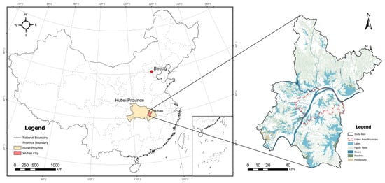
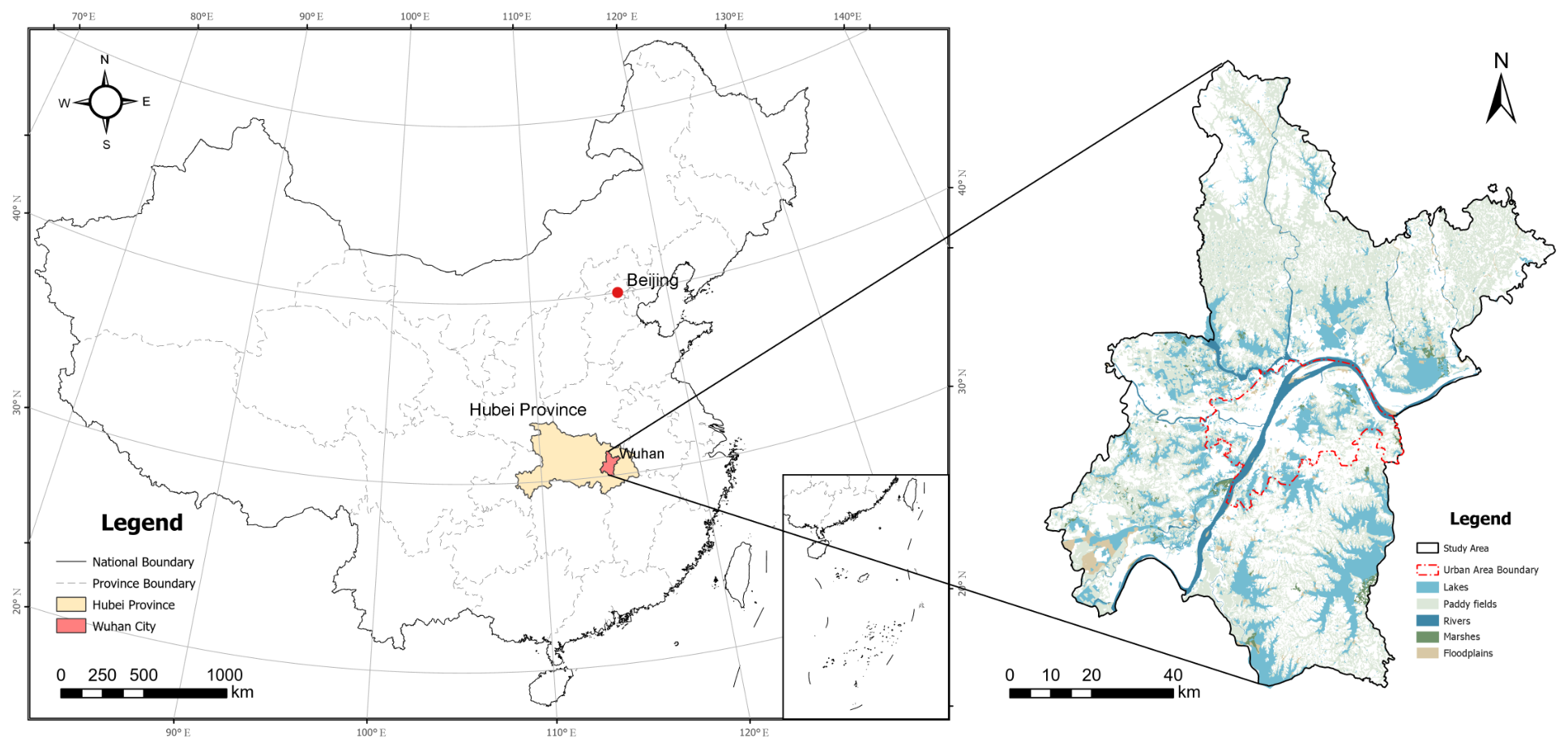
Wuhan (113°41′–115°05′ E, 29°58′–31°22′ N) is located in central China (Figure 1). It has a subtropical humid monsoon climate, with an annual mean temperature of approximately 16 °C and annual precipitation of approximately 1200 mm. Rich in wetland resources, Wuhan is a representative lake-wetland city in the middle and lower reaches of the Yangtze River [45]. In 2022, Wuhan was accredited as an International Wetland City under the Convention on Wetlands. Its natural wetlands cover approximately ha, accounting for 18.9% of the city’s total land area.
Figure 1.
Location of the study area.
As a major central city in China, Wuhan has undergone rapid urbanization. In 2023, its permanent resident population reached 13.774 million, its urban area reached 8569.19 km2, and its GDP reached CNY 2 trillion. Wuhan is characterized by a typical urban–wetland composite system, and economic development and urban expansion have substantially altered its wetland landscape patterns [46].
2.2. Data Sources and Processing
This study analyzed three time points: 2000, 2010, and 2020. The primary spatial datasets, source organizations, time points, and original resolutions are listed in Table 1. Wetland extent was extracted from the 30 m China multi-period land-use/land-cover remote-sensing monitoring dataset (CNLUCC). Wetland classes in this study comprise rivers and canals, lakes, reservoirs and ponds, paddy fields, marshes, and floodplains.
Table 1.
Primary spatial datasets used in this study.
All rasters were harmonized to the same projection, spatial extent, and 30 m pixel size. Ecosystem service models were first run for the entire administrative area of Wuhan, after which their outputs were masked to the wetland extent. Landscape pattern metrics were calculated with a 900 m moving window and aligned to the 30 m analysis grid.
2.3. Ecosystem Service Supply and Synergistic Benefit Indices
2.3.1. Assessment of Ecosystem Service Supply
InVEST (Integrated Valuation of Ecosystem Services and Tradeoffs), developed by the Natural Capital Project, is a spatially explicit tool for ecosystem service assessment. Using InVEST 3.14.3, we ran the Annual Water Yield, Nutrient Delivery Ratio (NDR), Sediment Delivery Ratio (SDR), and Habitat Quality modules at a 30 m resolution to estimate water yield (WY), water purification (WP), soil conservation (SC), and habitat quality (HQ), respectively. These services are representative indicators of wetland functions related to hydrological regulation, pollutant retention, soil maintenance, and habitat provision [2,11,47,48].
Model inputs and parameters followed the InVEST user guide and parameter choices reported in previous studies [49,50,51,52,53,54,55,56,57,58,59,60]; the values used here are described below. The Annual Water Yield module used land use, annual precipitation, potential evapotranspiration, plant-available water content, root-restricting layer depth, and a biophysical coefficient table as inputs. Annual pixel-level water yield depth was calculated using the Budyko water-balance framework, with the seasonal constant set to 12.7. Its principal water-balance expression is , where , , and are annual water yield, precipitation, and actual evapotranspiration at pixel x, respectively [56,57]. The NDR module calculated nitrogen export, which was used as an inverse indicator of water purification. At pixel level, total nitrogen export is the sum of surface and subsurface nitrogen loads multiplied by their respective delivery ratios; higher modeled nitrogen export therefore indicates a lower value of the WP proxy [58]. Surface and subsurface nitrogen loads and retention parameters were obtained from the biophysical coefficient table. Maximum subsurface retention efficiency was set to 0.8, critical subsurface flow length to 200 m, the connectivity parameter to , and the flow accumulation threshold to 500. The SDR module used a digital elevation model (DEM), rainfall erosivity, soil erodibility, land use, and a biophysical coefficient table as inputs. Soil conservation was derived from potential erosion, actual erosion, and sediment deposition. Specifically, , where is potential erosion without vegetation cover, is modeled actual erosion, and is downslope sediment trapping at pixel x [59]. Parameters were set to , , a maximum slope length of 122 m, a maximum sediment delivery ratio of 0.8, and a flow accumulation threshold of 1000. The Habitat Quality module used threat sources and a land-use sensitivity table. The quality score follows , where is habitat suitability, is degradation, , and k is the half-saturation constant [60]. The model-default scaling constant of 2.5 was used. Following the official InVEST guide, an initial run with default parameters was conducted for each year to obtain the maximum degradation score, and that year’s half-saturation constant was set to half the maximum. The resulting constants were 0.3453, 0.3494, and 0.353 for 2000, 2010, and 2020, respectively.
Because the four services differ in units and direction, min–max normalization was performed separately within each year. WY, SC, and HQ were treated as positive indicators, whereas nitrogen export was treated as an inverse indicator, so a higher normalized WP value represents lower modeled nitrogen export. The raw, unnormalized outputs retain their original units and were used to compare a given service across years; the normalized outputs were used to construct each year’s ESS, EST, and ESB.
2.3.2. Ecosystem Service Synergistic Benefit Index
To characterize overall synergy among wetland ecosystem services, we calculated the ecosystem service composite benefit index (ESS), overall trade-off index (EST), and synergistic benefit index (ESB) in sequence. First, the four normalized ecosystem service results were averaged to obtain ESS, which represents the overall supply capacity across multiple services. Second, EST was calculated using the root mean square deviation (RMSD) to characterize disparities among services. Finally, ESS and EST were combined into ESB, representing both overall supply capacity and the degree of synergy among services [61,62,63].
ESS measures the overall supply capacity of multiple ecosystem services as a weighted mean [61,63]. Equal weights were used in this study, and ESS was calculated as follows:
where is the normalized value of ecosystem service i, is its weight, and n is the number of ecosystem services. A higher ESS indicates stronger overall wetland ecosystem service supply.
EST characterizes disparities among ecosystem services and thereby reflects the intensity of trade-offs. RMSD was used to quantify the dispersion of each service relative to the mean across services [61,62]. A higher EST indicates a less balanced service supply; a value of 0 indicates that the four normalized service values are identical. Under Equation (2) and the condition that all four values lie within , the theoretical range of EST is . EST is an operational measure of service balance in this study and was calculated as follows:
where is the normalized value of ecosystem service i, is the mean across all ecosystem services, and n is the number of services.
Finally, ESB was introduced on the basis of ESS and EST to jointly represent overall supply capacity and the synergistic state among ecosystem services [63]. It is a constructed composite score that favors relatively high aggregate supply together with a more balanced service profile; balance alone cannot yield a high score when supply is low. This choice follows the multiple-objective benefit and trade-off framework of Bradford and D’Amato [61]. ESB ranges from 0 to 1; higher values indicate stronger synergy while maintaining a relatively high level of supply. It was calculated as follows:
2.4. Landscape Patterns
2.4.1. Landscape Pattern Metrics
Landscape pattern metrics quantitatively characterize the composition and spatial configuration of landscape structure. They condense spatial information on land use into comparable numerical indicators, thereby revealing characteristics such as fragmentation, aggregation, and shape complexity.
Many landscape pattern metrics are redundant. Including all available metrics would increase the computational burden and could introduce multicollinearity, undermining the stability of regression analysis. To quantify associations of landscape-pattern change with ESs and ESB, we used collinearity diagnostics to select five core metrics (Table 2): aggregation index (AI), contagion index (CONTAG), largest patch index (LPI), patch density (PD), and mean shape index (SHAPE) [64,65]. Table 3 reports Pearson correlation coefficients and variance inflation factors (VIFs) for the five metrics. Three VIFs were below 5; PD (5.20) and AI (8.99) showed greater information overlap, but neither exceeded the empirical multicollinearity-risk threshold of 10 proposed by the US National Institute of Standards and Technology (NIST). The five metrics were calculated as follows.
where is the observed number of like adjacencies between patches of class i, and is the maximum possible number of like adjacencies for the given number of patches. Higher values indicate greater aggregation [64,66].
where is the proportion of all adjacent cell pairs in which patch types i and j co-occur, and m is the total number of patch types. The value approaches 0 when all patch types are maximally fragmented and isolated, and approaches 100 when they are maximally aggregated [64,67].
where is the area of the largest patch and is the total landscape area. Higher values indicate that the largest patch occupies a greater proportion of the landscape [64].
where is the total number of patches, is the total landscape area, and K is a conversion factor that expresses the unit as the number of patches per 100 ha. Higher values indicate more patches per unit area and greater landscape fragmentation [64].
where is the total number of patches, and and are the perimeter and area of patch i, respectively. A value of 1 indicates a perfectly circular patch with the shortest possible boundary; values above 1 indicate increasing deviation from a circle and greater shape and boundary complexity [64].
Table 2.
Landscape pattern metrics and their ecological meanings.
Table 3.
Pearson correlation coefficients and variance inflation factors for the landscape pattern metrics.
2.4.2. Scale Effects of Landscape Patterns
Wetland landscape pattern metrics exhibit pronounced scale effects [68]; that is, the same landscape characteristic may be expressed differently across spatial scales [69]. Selecting a scale that retains essential information while avoiding noise and redundancy is therefore a prerequisite for accurately quantifying landscape patterns [70]. Semivariograms are widely used to quantify differences, or dissimilarity, in spatial data as a function of distance and can effectively describe the relationship between landscape pattern metrics and spatial variability [71]. We combined moving-window analysis with semivariograms to validate the spatial variability of landscape pattern rasters generated using different window sizes. This allowed us to quantify the scale sensitivity of wetland landscape patterns in Wuhan and identify an appropriate spatial scale. The semivariogram is defined as follows:
where is the number of sample pairs separated by distance h, and is the metric value at sample location . As h increases, spatial correlation between sample points gradually weakens, and increases before eventually stabilizing [71].
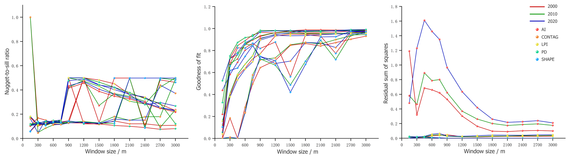
Three complementary measures were used for evaluation: the nugget-to-sill ratio, coefficient of determination (), and residual sum of squares (RSS). Lower nugget-to-sill ratios and RSS values, together with higher , indicate that the spatial variation is better explained.
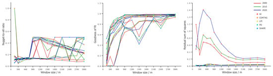
As shown in Figure 2, increased with window size and gradually stabilized, with only small gains beyond 900 m. RSS declined as window size increased and stabilized near 1200 m. Because the original data resolution was 30 m, an excessively large window could obscure local detail. Balancing representation of spatial structure, information fidelity, and computational efficiency, we selected 900 m for subsequent landscape pattern calculations. An approximately 1-km spatial extent is commonly used to characterize the surrounding landscape context in assessments of ecosystem services and wetland-related ecological functions [72,73,74,75]. Although this window has not been validated as the optimal ecological response scale for each service, it represents a compromise for comparing associations across services.
Figure 2.
Semivariogram fit diagnostics for landscape pattern metrics across moving-window scales.
2.5. Explainable Machine-Learning Models
The explanatory variables in the machine-learning analysis were AI, CONTAG, LPI, PD, and SHAPE, and the response variables were WY, WP, SC, HQ, and ESB.
First, we compared the predictive performance of Random Forest, LightGBM, and XGBoost. Grid search was used to find the optimal hyperparameters. The final settings were 300 trees for Random Forest, and 500 trees, a learning rate of 0.05, and a maximum depth of 5 for both XGBoost and LightGBM. The coefficient of determination (), root mean square error (RMSE), and mean absolute error (MAE) were used to evaluate training-set fit and test-set prediction and to select the model for subsequent interpretation.
XGBoost is a gradient-boosted decision-tree ensemble algorithm [76] capable of modeling complex nonlinear relationships. To interpret XGBoost predictions, SHAP (Shapley additive explanations) was used to calculate the marginal contribution of each landscape metric to the prediction for each sample. The Shapley value is defined as follows:
where p is the total number of features, N is the full feature set, and S is a subset that does not include feature j. SHAP summary plots were used to assess the magnitude and direction of feature contributions. The relative contribution of each feature was obtained by normalizing its mean absolute SHAP value.
To identify candidate turning points in the response curves, locally weighted regression (LOWESS) was fitted to the feature-value–SHAP-value scatterplot for each feature. Sign changes between adjacent smoothed values were then used to locate intersections with , and interpolation and numerical root finding were applied to calculate their positions. This procedure identifies candidate turning points at which the model contribution changes from negative to positive or vice versa.
3. Results
3.1. Spatial Characteristics of Landscape Patterns
3.1.1. Changes in Wetland Area and Distribution
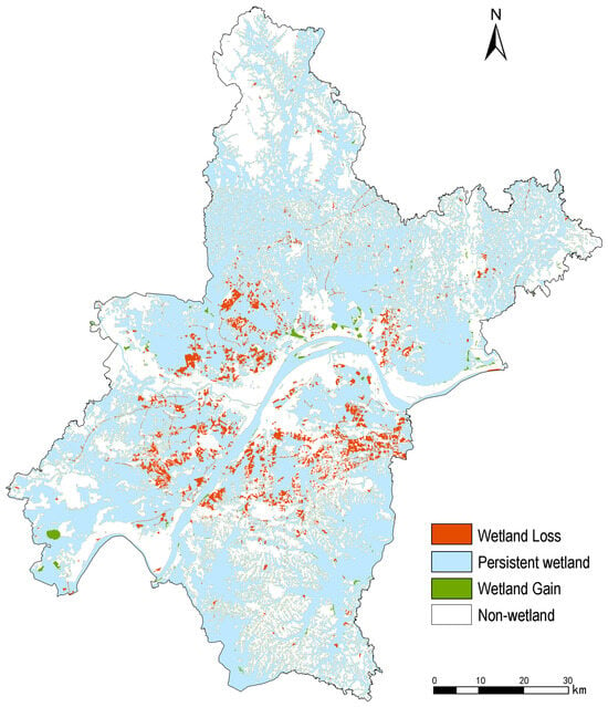
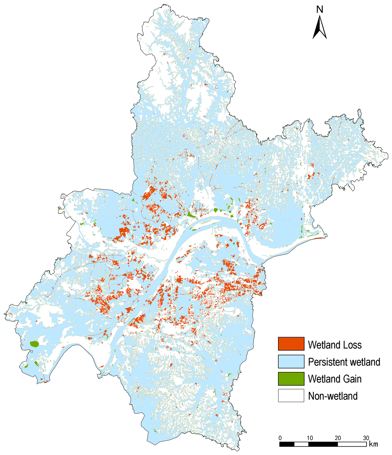
Wetland area in Wuhan declined during the study period (Figure 3). The total wetland area decreased by 5.83%, or approximately 300 km2 (Table 4). Among natural wetland types, floodplain wetlands experienced the greatest loss, concentrated in and around built-up areas. Newly formed wetlands were limited and were distributed mainly in suburban and riverfront areas, where they were associated with riverfront improvement and ecological restoration projects. Overall, wetland degradation spread outward from the central urban area.
Figure 3.
Spatial distribution of wetland changes in Wuhan.
Table 4.
Changes in the area of different wetland types in Wuhan.
3.1.2. Changes in Wetland Landscape Patterns
Table 5 presents the wetland landscape pattern metrics for the entire Wuhan municipality from 2000 to 2020. AI declined from 95.81% in 2000 to 95.42% in 2020, indicating weakened patch aggregation and declining landscape connectivity. Consistent with this change, CONTAG decreased from 59.03% to 58.54%, suggesting reduced aggregation among patch types and increased spatial heterogeneity in the wetland landscape. LPI declined from 66.29% to 64.25%, indicating that the dominance of the largest wetland patch gradually weakened and that the dominant landscape structure became more diverse. Meanwhile, PD increased continuously from 6.26 to 6.80 , showing an increase in the number of patches per unit area and greater landscape fragmentation. This pattern reflects the division and encroachment of wetlands under urban expansion. SHAPE increased slightly from 1.36 to 1.37, indicating a modest increase in shape complexity and more irregular patch boundaries, potentially related to irregular subdivision caused by human disturbance and land development. Overall, wetland landscapes in Wuhan became more fragmented, less connected, and morphologically more complex over the study period, reflecting sustained disturbance to wetland ecological space during urbanization.
Table 5.
Changes in wetland landscape pattern metrics in Wuhan.
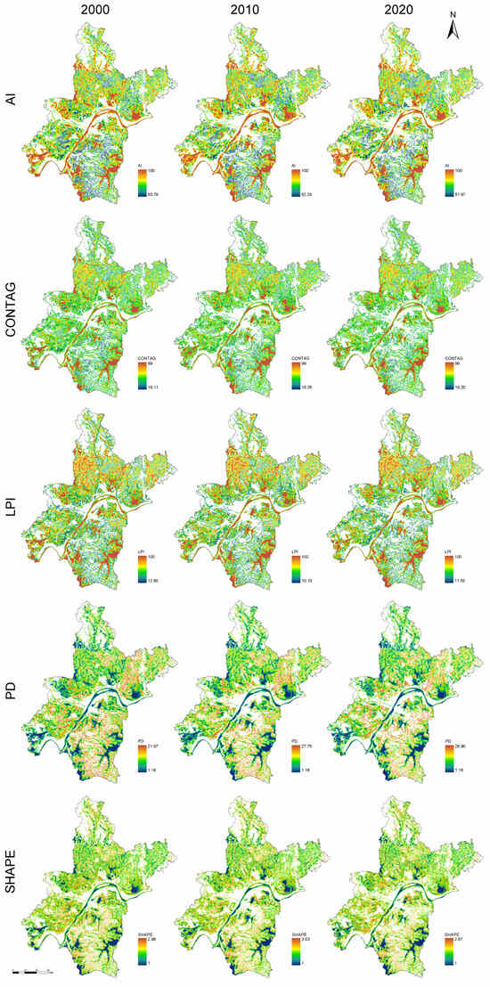
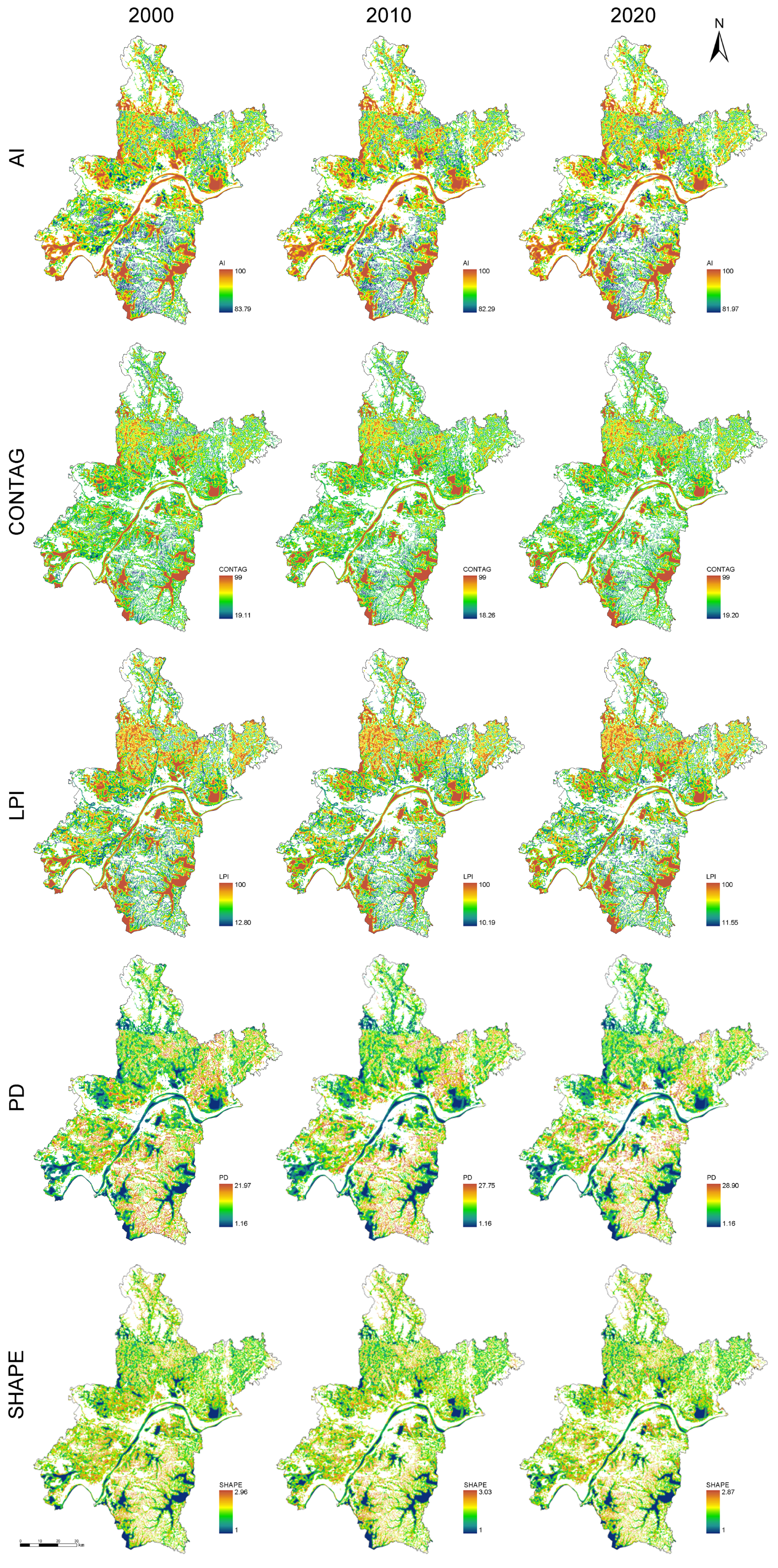
Figure 4 presents the spatial distributions of wetland landscape pattern metrics in Wuhan from 2000 to 2020, calculated using a 900 m moving window and represented at a 30 m pixel resolution. High AI values were concentrated in outlying suburban areas dominated by large lake wetlands, whereas wetland aggregation declined in the central urban area. CONTAG was generally low and decreased over time, indicating a gradual weakening of wetland connectivity and integrity. High LPI values were concentrated around large lakes and riparian wetlands, but declined over time, suggesting reduced dominance of the largest wetland patches. PD generally increased, particularly in areas undergoing marked urban expansion, showing that wetland patches were subdivided into smaller units and became increasingly fragmented. SHAPE increased in some urban-fringe and small wetlands, indicating more complex and irregular patch shapes under human influence.
Figure 4.
Spatial distribution of changes in wetland landscape patterns in Wuhan.
3.2. Spatiotemporal Patterns and Changes in Wetland Ecosystem Services
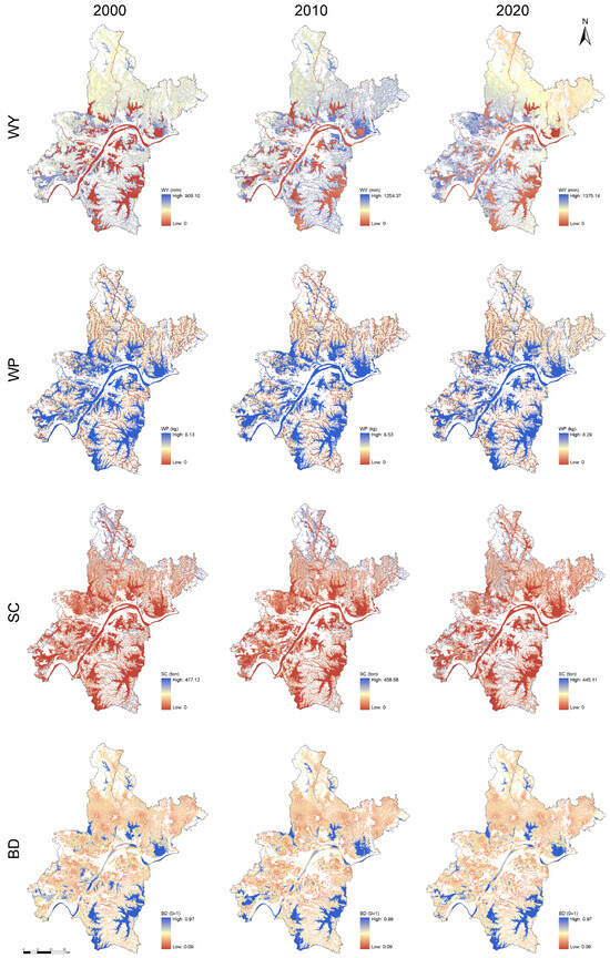
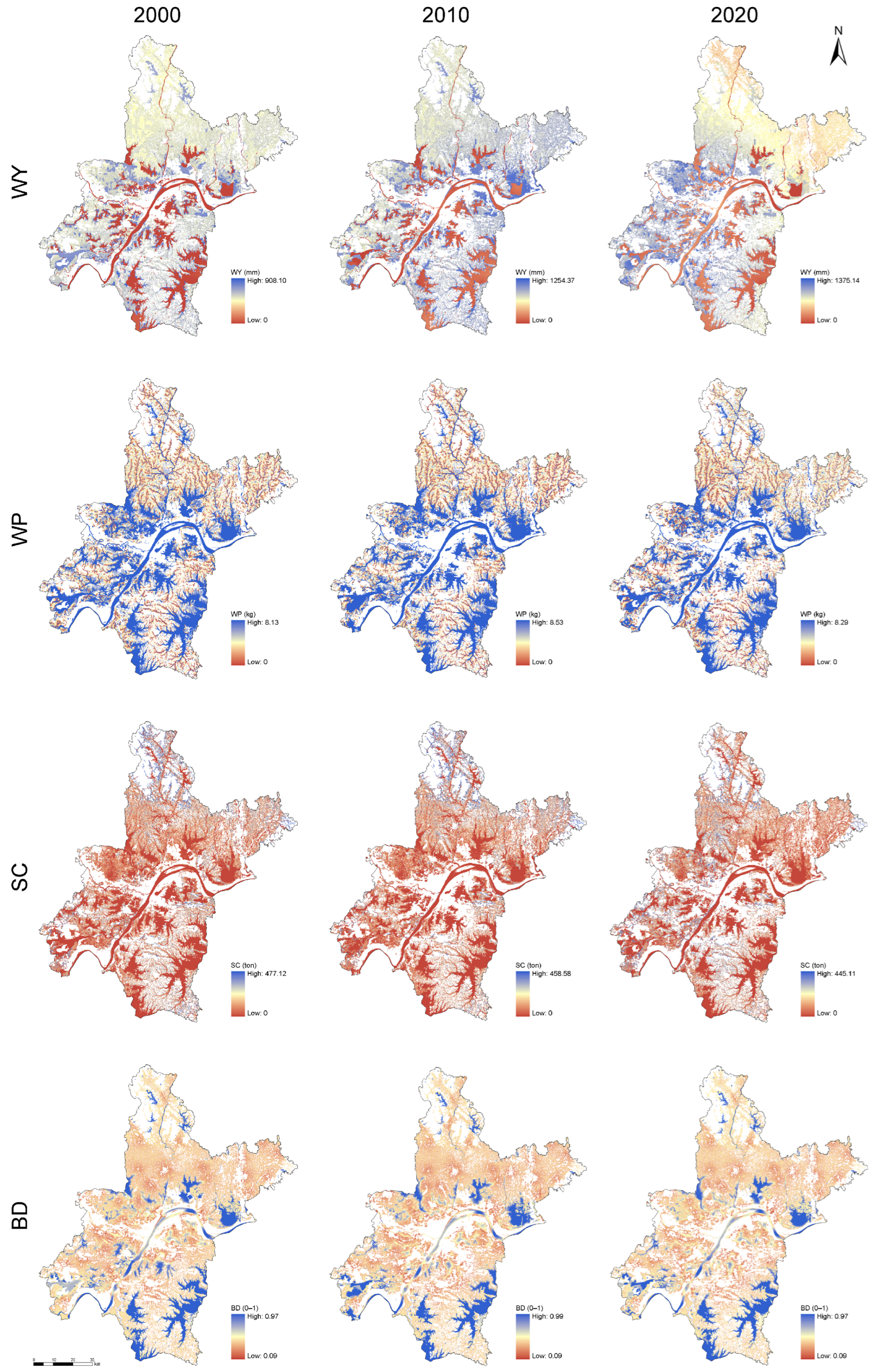
Figure 5 shows pronounced spatial heterogeneity in wetland ecosystem service supply across Wuhan. High WY values occurred mainly in hilly and mountainous wetlands in the southeast and southwest, whereas values were generally low in the central urban area. High WP values were concentrated in natural wetlands along the main channel of the Yangtze River and its major tributaries. The highest SC values occurred in the northeastern hills and southern mountains, whereas supply was comparatively weak across the plains. High HQ values were found primarily in suburban wetlands, riparian wetlands, and some artificial wetlands, whereas values were generally low around urban areas and in scattered small wetland patches.
Figure 5.
Wetland ecosystem services in Wuhan.
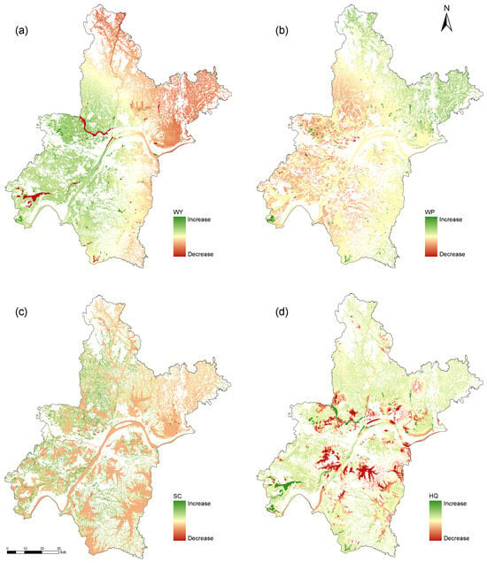
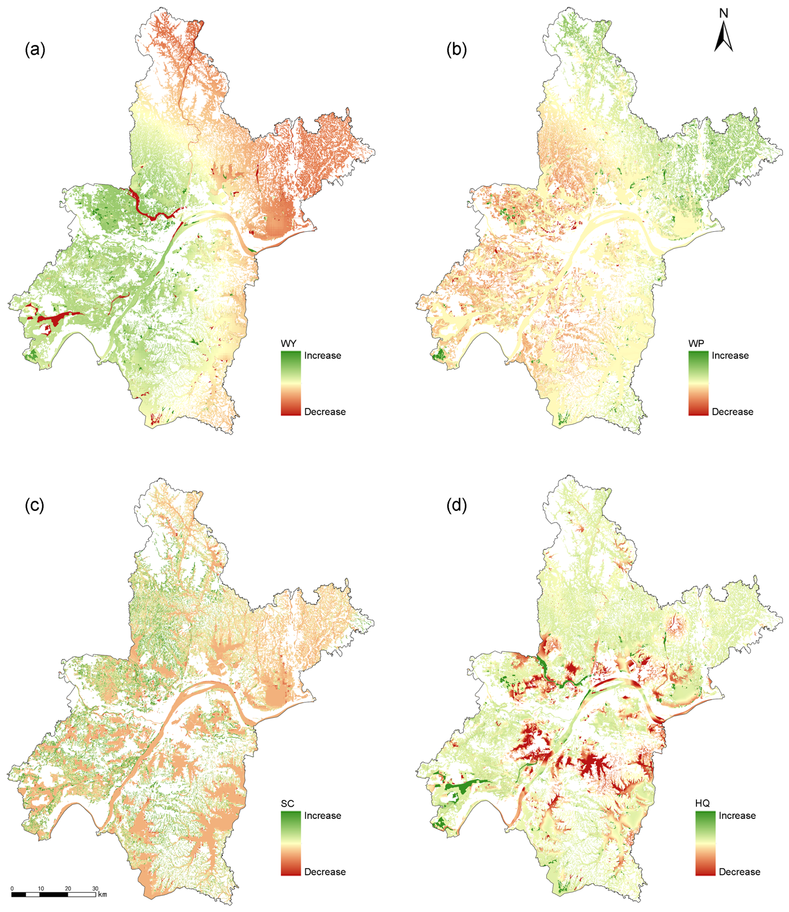
Figure 6 shows changes in the four WESs over the study period. WY increased in the southwest and in some suburban areas but generally declined in the central urban and northern areas. WP improved slightly around urban areas and in some dense drainage networks, but declined in built-up areas and parts of the upstream region. SC decreased overall, with particularly marked degradation in the southern and eastern hills. Declines in HQ were concentrated along urban development corridors and in ecologically sensitive areas in the south, whereas some outer suburban areas improved. Overall, WESs in Wuhan exhibited a pattern of decline in urban areas and variable change in suburban areas, revealing the sustained influence of urbanization on wetland ecological functions.
Figure 6.
Changes in wetland ecosystem services in Wuhan: (a) water yield; (b) water purification; (c) soil conservation; and (d) habitat quality.
3.3. Spatial Patterns of Composite Wetland Ecosystem Service Indices
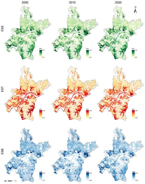
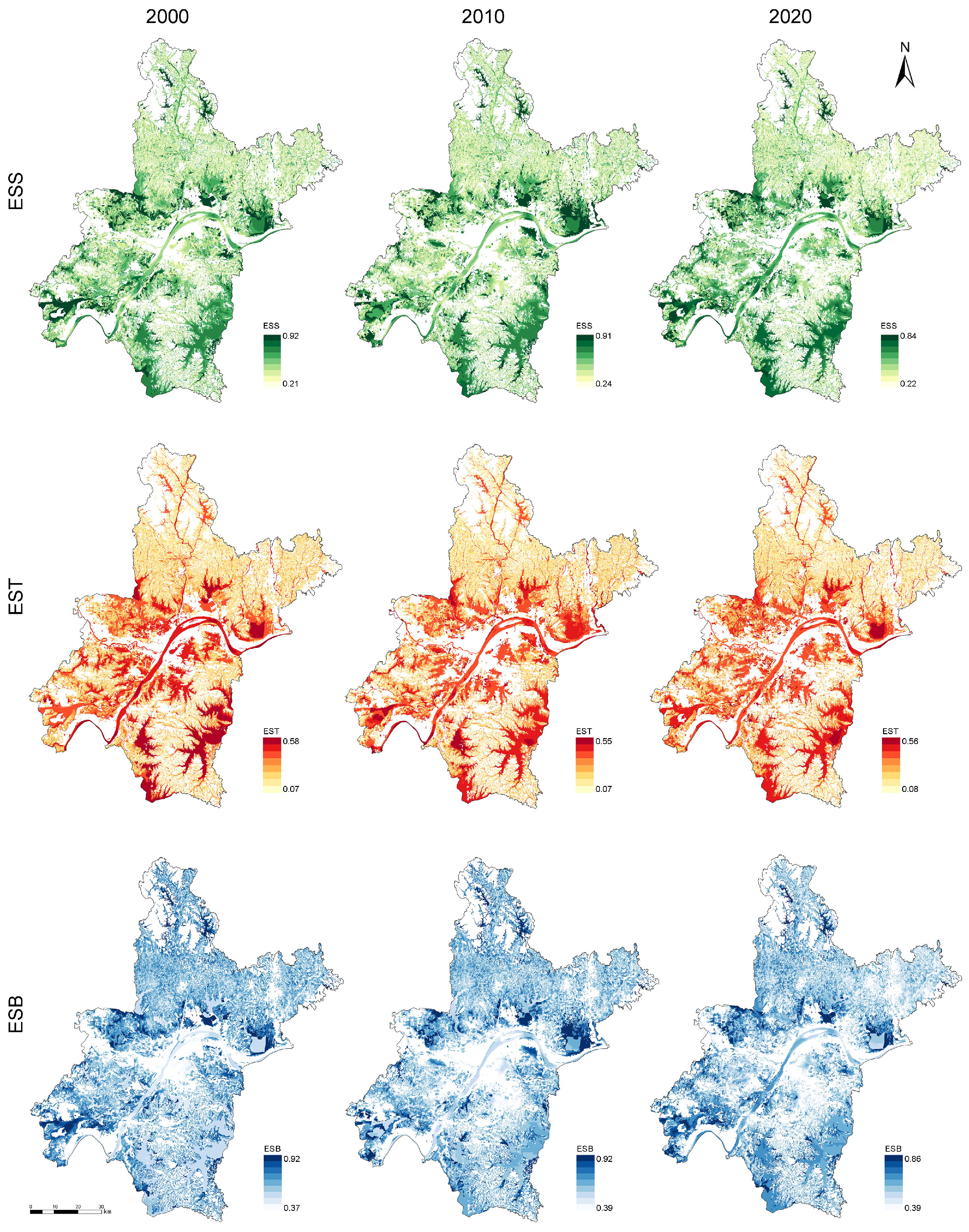
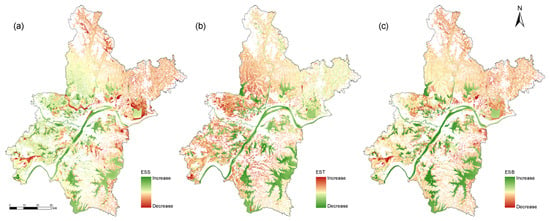
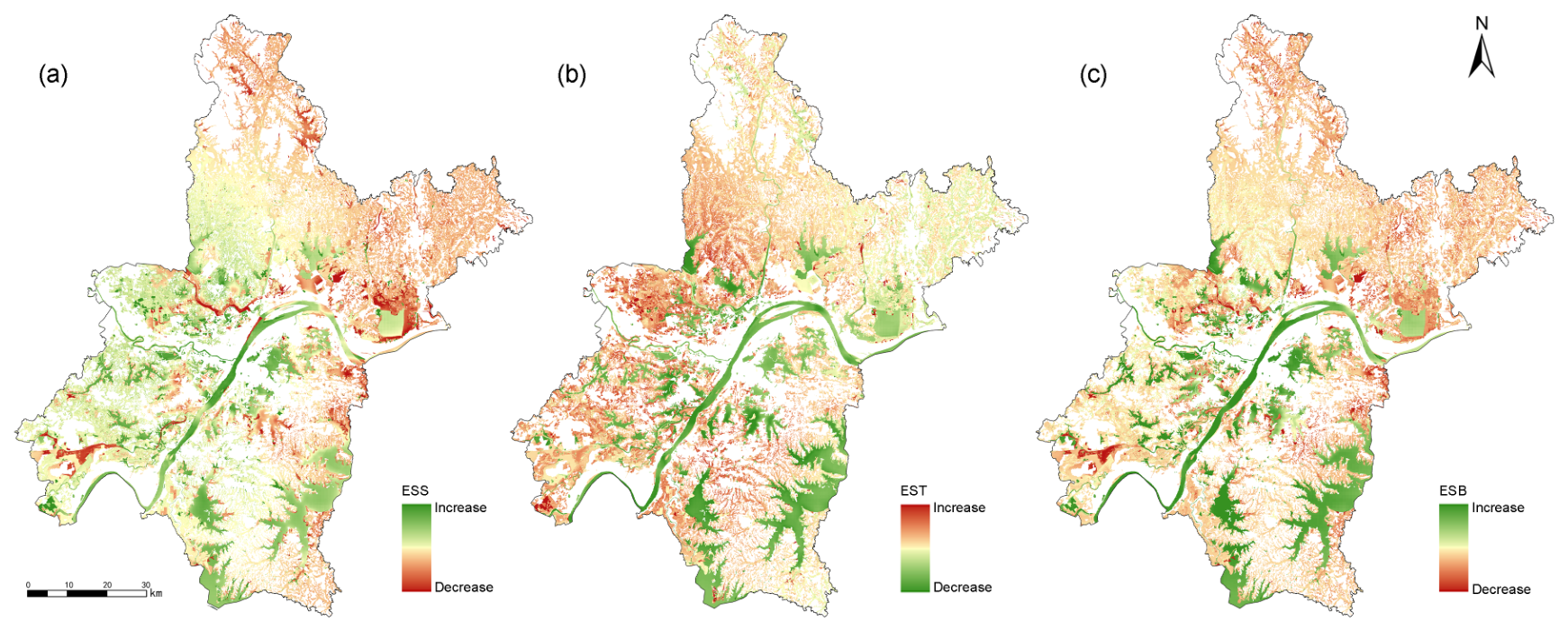
Figure 7 and Figure 8 show the spatial patterns of the composite benefit index (ESS), overall trade-off index (EST), and synergistic benefit index (ESB) for wetlands in Wuhan from 2000 to 2020. ESS was generally higher in the south than in the north. Large lakes and river or canal wetlands had relatively strong supply capacity, whereas ESS was markedly lower in the central urban area and fragmented landscapes. High EST values occurred mainly in built-up and fragmented wetland areas. High ESB values were concentrated in large lakes and well-connected wetland patches, whereas low values occurred mainly around the urban core.
Figure 7.
Composite wetland ecosystem service indices in Wuhan.
Figure 8.
Spatial patterns of changes in composite wetland ecosystem service indices in Wuhan: (a) ESS; (b) EST; and (c) ESB.
3.4. Model Validation
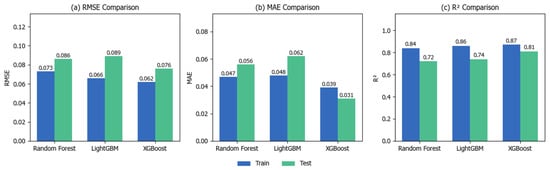
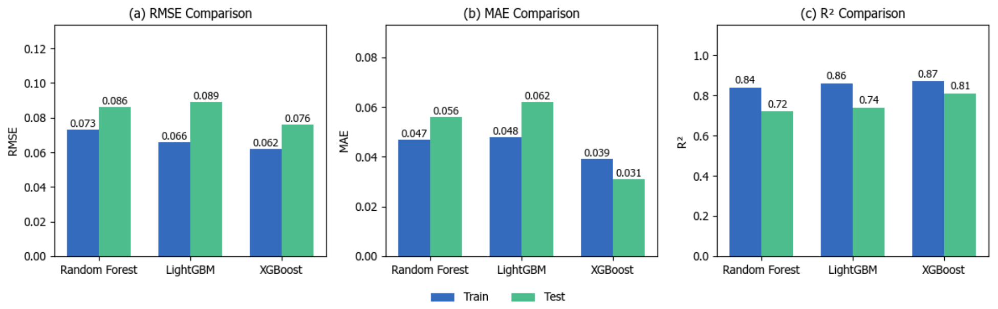
The predictive performance of Random Forest, LightGBM, and XGBoost was compared using RMSE, MAE, and (Figure 9). Random training and test sets were established at a ratio of 80% to 20%. XGBoost performed best among the three models: its training- and test-set RMSE values were 0.062 and 0.076, its MAE values were 0.039 and 0.031, and its values were 0.87 and 0.81, respectively. Compared with Random Forest and LightGBM, XGBoost reduced test-set RMSE by 11.6% and 14.6%, respectively, and increased test-set by 0.09 and 0.07, respectively.
Figure 9.
Performance comparison of XGBoost, Random Forest, and LightGBM under a random split.
The training/test values were 0.84/0.72 for Random Forest and 0.86/0.74 for LightGBM, and both models showed larger performance gaps between the training and test sets than XGBoost. Overall, XGBoost demonstrated a relatively strong fit and test-set predictive performance for the randomly split samples used in this study and was therefore selected as the basis for the subsequent SHAP interpretation.
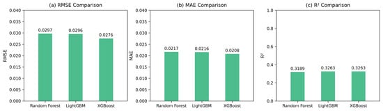
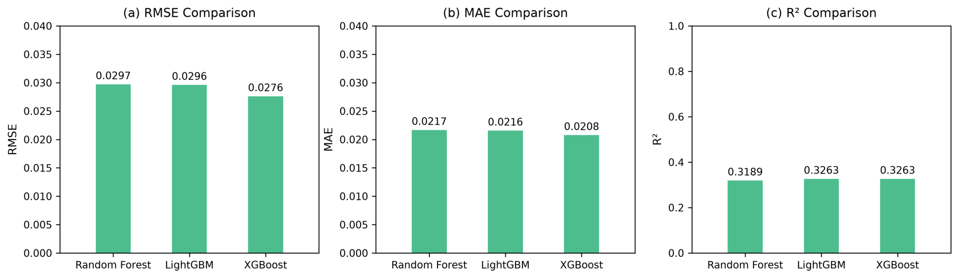
Previous research has found that ordinary random cross-validation can substantially overestimate the predictive performance of tree models on spatial data [77]. We therefore also performed fivefold spatial-block holdout validation of XGBoost using the same sample data (Figure 10).
Figure 10.
Performance comparison of XGBoost, Random Forest, and LightGBM under a spatial block split.
3.5. Landscape-Pattern Correlates of Wetland Ecosystem Services
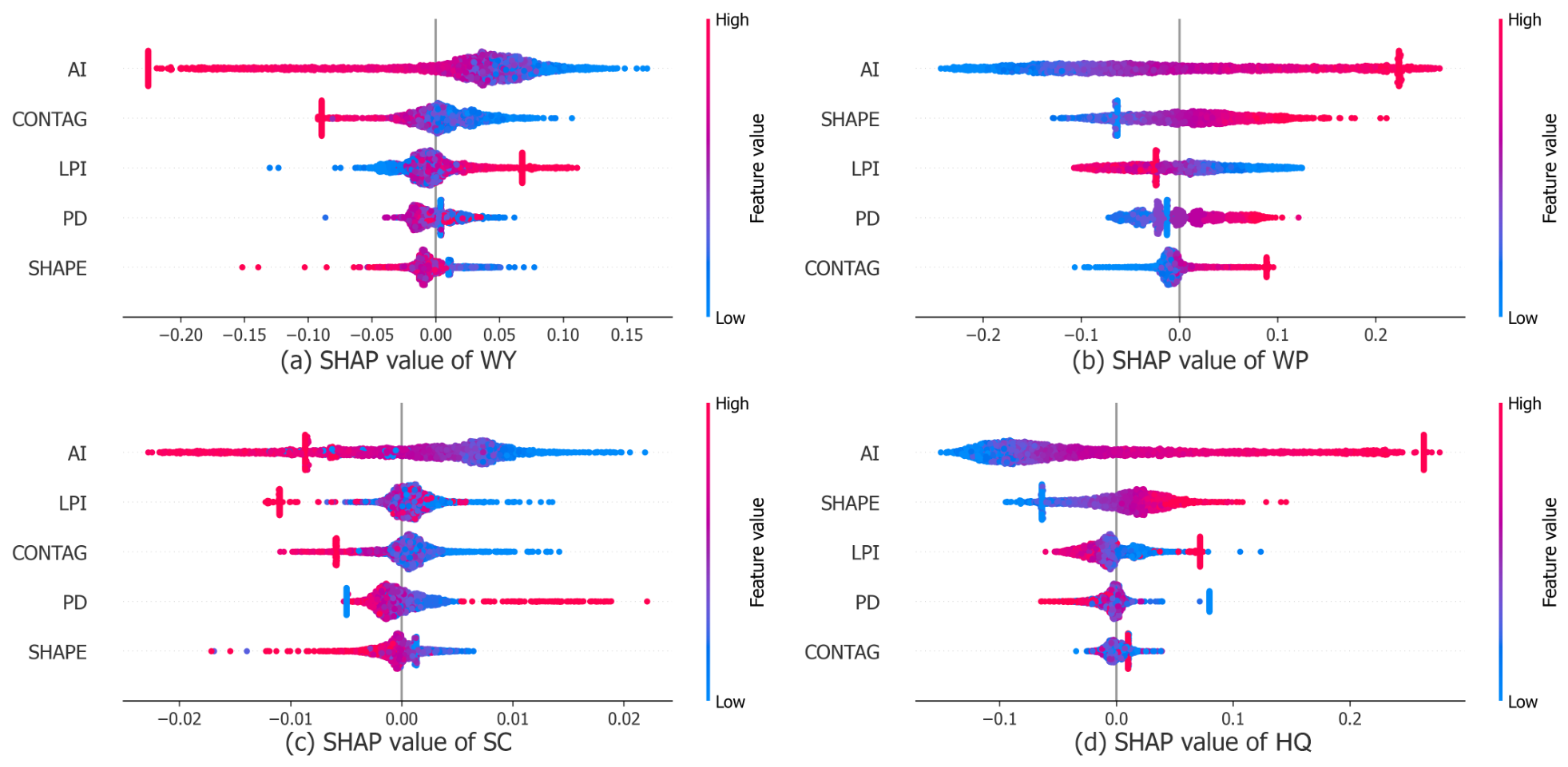
To identify the principal correlates of different WESs, SHAP summary plots were used to compare the relative contributions of the five landscape pattern metrics to predictions of WY, WP, SC, and HQ (Figure 11). Overall, AI and SHAPE had large absolute SHAP values in most service models, indicating that patch aggregation and edge complexity provided important information for model predictions. LPI also contributed substantially, whereas the contributions of CONTAG and PD were relatively weak or varied considerably among services.
Figure 11.
SHAP summary plots of landscape pattern metrics for four wetland ecosystem services: (a) water yield (WY); (b) water purification (WP); (c) soil conservation (SC); and (d) habitat quality (HQ).
Regarding the direction of the associations, AI and LPI more frequently made positive SHAP contributions in the WY and SC models, indicating that more aggregated and continuous spatial patterns or landscapes dominated by large patches were associated with higher predicted water yield and soil conservation. SHAPE and AI more frequently made positive contributions in the WP and HQ models, suggesting that edge complexity and spatial aggregation may be associated with spatial differences in nutrient retention and habitat quality.
3.6. Relative Importance of Landscape Pattern Metrics to Wetland ESB
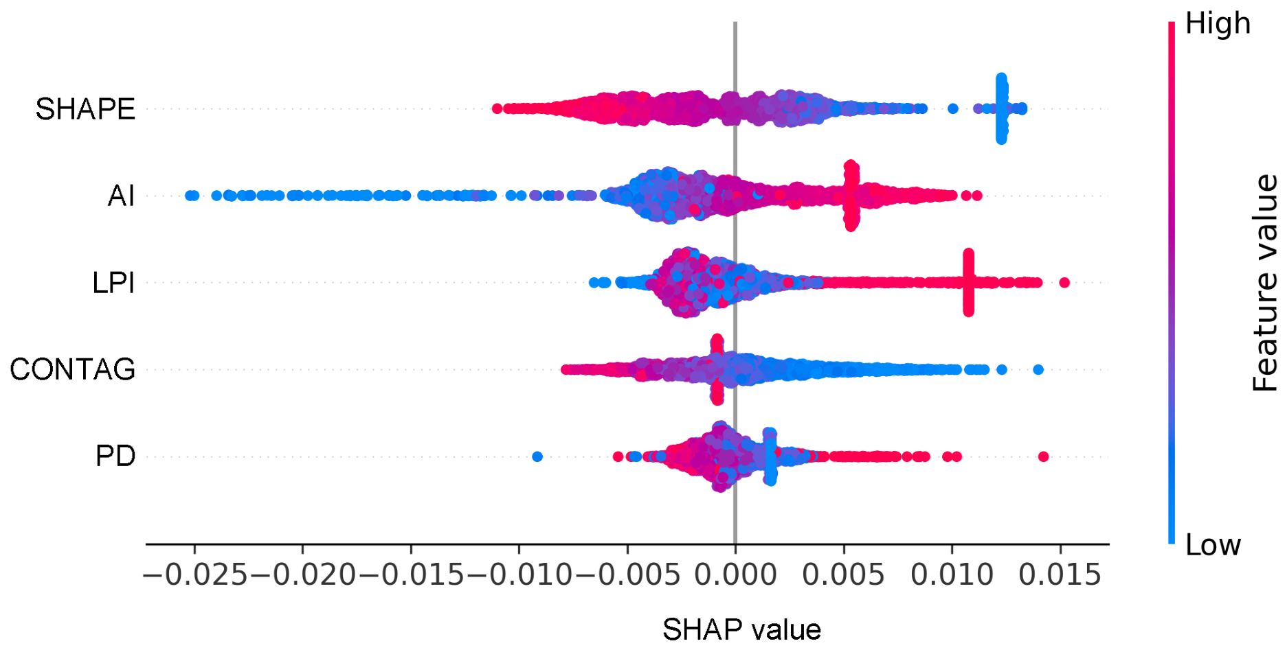
The effects of landscape pattern metrics on ecosystem service synergy differed substantially during wetland landscape change. Figure 12 shows the importance ranking derived from XGBoost and SHAP. Each point represents a feature value in the dataset, with colors from red to blue indicating high to low feature values. The horizontal axis represents the SHAP value: positive values indicate positive contributions to the predicted response and negative values indicate negative contributions; points clustered near a SHAP value of 0 indicate small contributions to model predictions.
Figure 12.
Relative importance of landscape pattern metrics in the ESB model.
Table 6 reports the relative contributions of the core explanatory variables. SHAPE contributed the most (25.56%), followed by AI (21.00%) and LPI (19.54%). CONTAG and PD contributed 18.86% and 15.04%, respectively. Together, SHAPE, AI, and LPI accounted for approximately 66.10% of the total contribution, indicating that wetland edge complexity, aggregation, and the dominance of wetland patches in the regional landscape were key landscape attributes associated with wetland ecosystem service synergy.
Table 6.
Relative contributions of landscape pattern metrics to the model.
3.7. Nonlinear Associations Between Landscape Patterns and Ecosystem Service Synergy
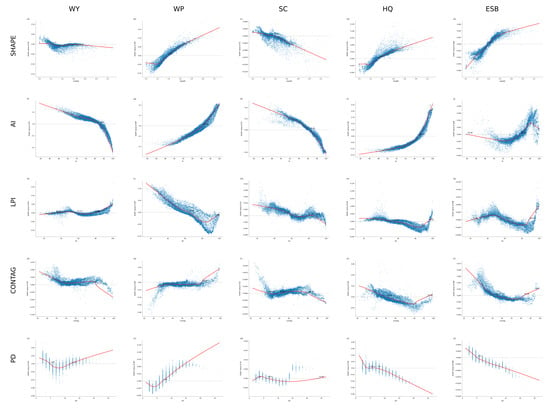
Figure 13 shows the SHAP dependence curves from the XGBoost models. All five landscape pattern metrics exhibited some degree of nonlinearity in their model responses for wetland ESs and ESB, with relatively distinct candidate turning-point ranges for SHAPE, AI, and LPI.
Figure 13.
SHAP dependence plots. Rows show SHAPE, AI, LPI, CONTAG, and PD, and columns show WY, WP, SC, HQ, and ESB. Blue points represent individual samples, red lines show LOWESS-smoothed relationships, and blue markers indicate where the smoothed curves cross zero.
Several SHAPE curves changed direction near 1.2–1.4. The SHAP contributions to WY and SC changed from positive to negative, whereas those to WP and HQ changed from negative to positive. The ESB curve changed from a negative to a positive contribution at approximately 1.40.
Candidate turning points for AI were concentrated around 96%. The SHAP contributions to WY and SC generally decreased as AI increased, whereas those to WP and HQ generally increased. The ESB contribution changed from negative to positive at approximately 95.9%, after which the rate of increase diminished. The vicinity of 96% may therefore be treated as a reference turning-point range.
The LPI responses were more complex. The contribution to WY gradually became positive as LPI increased, whereas those to WP and HQ generally declined. The central crossing of the ESB curve was near 61%. This nonmonotonic relationship suggests that intermediate proportions of large patches and very high proportions of core patches may correspond to different spatial-structural states.
4. Discussion
4.1. Associations Between Landscape Patterns and WESs
Our results (Figure 12) show that landscape pattern metrics provide important explanatory information in the wetland ESB model, consistent with previous findings that landscape structure is closely related to ecosystem services [16,78,79]. The relatively large contributions of SHAPE, AI, and LPI indicate strong nonlinear associations of ESB spatial variation with edge complexity, patch aggregation, and dominance of the largest patch.
Aggregation was positively associated with ESB and contributed positively to several ESs, particularly WP and HQ (panels g and i in Figure 13). Highly aggregated wetland patches may provide longer flow paths and more opportunities for pollutant retention, thereby increasing nitrogen retention [80]. They may also form continuous habitat corridors that facilitate the movement of fish, amphibians, and birds through wetland landscapes [81]. Increased wetland aggregation may therefore strengthen water purification and improve habitat quality. Although this result is consistent with previous findings that continuous, aggregated wetland landscapes help sustain wetland functions and services [82,83,84], the proposed hydrological and connectivity mechanisms remain hypotheses based on ecological theory and require further validation. At very high aggregation levels, however, the responses of WY and SC to AI became negative (panels f and h in Figure 13), suggesting that excessive homogenization may weaken hydrological regulation and soil retention.
Wetland fragmentation has often been regarded as an indicator of ecological degradation [81,85,86]. Our results, however, suggest that moderate increases in wetland edge complexity and patch heterogeneity may, under certain conditions, favor the supply and synergy of wetland ecosystem services. Higher SHAPE and intermediate LPI values were associated with higher predicted ESB values (panels e and o in Figure 13) and with higher predicted values of some individual ESs (panels b, d, and k–n in Figure 13). Edge effects provide one possible ecological explanation: longer and more convoluted land–water interfaces may support greater biodiversity and population density and enhance pollutant retention, nutrient transformation, and the availability of suitable habitat sites [87], thereby benefiting water purification and biodiversity. Greater heterogeneity may also create diverse microenvironments and energy-flow pathways that support the coexistence of different biological communities [88]. The same SHAPE value may, however, represent a naturally sinuous shoreline or an artificial edge, with potentially different ecological consequences. Another possible explanation for the nonmonotonic LPI curve is that intermediate dominance by a large patch may coexist with a network of smaller wetlands, whereas very high dominance may represent a few extensive and intact water bodies. Wetland type may also influence this apparent pattern.
This result differs from some previous findings for two possible reasons. First, the diversity and complexity of ESs generate intricate relationships among services [89,90]. Previous studies have generally focused on how landscape-pattern change affects the supply of individual WESs and have less often integrated the complex relationships among multiple services [11]. At the individual-service level, edge complexity and patch heterogeneity may negatively affect some services [91]; when evaluated using ESB, however, these structural attributes may exert an overall positive effect by promoting synergy among services. Second, the effects of edge complexity and heterogeneity on ESs are nonlinear and may exhibit threshold behavior. Moderate complexity and heterogeneity may enhance ESB (panels e and o in Figure 13), whereas values beyond a turning point may increasingly expose WESs to the adverse effects of fragmentation. Wetland fragments with complex edges may therefore function as either beneficial or risk-enhancing landscape elements, depending on whether the landscape pattern lies within a suitable range. Management should accordingly avoid both excessive fragmentation and oversimplified boundaries; maintaining moderate aggregation and appropriate edge heterogeneity may improve ES supply and ESB.
Although SHAPE, AI, and LPI were key factors associated with wetland ESs and ESB overall, individual services did not respond identically to changes in landscape-pattern characteristics. Some services benefited from greater edge complexity and aggregation, whereas others exhibited the opposite response. This variation complicates the relationships between landscape patterns and WESs and indicates that a positive effect on one service may coincide with negative effects on others. Divergent responses among wetland services therefore warrant further examination.
4.2. Divergent Responses Among Wetland Ecosystem Services
Further analysis showed that ecosystem services did not respond uniformly to landscape-pattern change but instead exhibited pronounced divergence (Figure 13). WY and SC showed highly similar response directions, as did WP and HQ. These two service groups often responded in opposite directions to the same pattern metric. For example, as aggregation increased, the water-purification–habitat group benefited, whereas the water-regulation–soil-conservation group was generally suppressed.
These differences can be explained by the dominant ecological processes underlying each service. Wetland water yield and soil conservation are driven primarily by hydrological processes, particularly precipitation [92,93], whereas water purification and habitat quality depend more strongly on biogeochemical cycling, biodiversity, and connectivity [94,95]. These processes differ in spatial scale [96], material-flow direction [97], and operative range [98], and may therefore cause landscape-pattern change to affect the two service groups differently or even in opposite directions.
This finding suggests potential risks from oversimplified wetland restoration policies. Overemphasizing a single structural characteristic may improve one group of services at the expense of another. For example, maximizing wetland patch aggregation may strengthen water purification and habitat functions but weaken water regulation and soil conservation. Conversely, focusing exclusively on overall connectivity and large-patch structure may limit the beneficial edge effects on purification and habitat. Wetland landscape management should therefore move beyond a single-service perspective and use ESB as an integrative objective that accounts for divergent responses among service groups.
4.3. Candidate Turning-Point Ranges and Management Implications
The divergent responses described above indicate that model associations between landscape pattern metrics and wetland ESB may change direction within particular value ranges. Relatively stable turning points occurred near SHAPE 1.40, AI 96%, and LPI 61%. Although these values are not absolute ecological thresholds with a causal interpretation, they can serve as reference thresholds for identifying priority areas and developing restoration strategies.
For management applications, priority attention may be given to wetland patches with SHAPE near 1.40, AI near 96%, and LPI near 61%, followed by field assessment of wetland type, location, and current service levels. For wetlands outside these ranges, corridor connections, buffer-zone configuration, and patch-structure optimization may be considered as possible ecological restoration measures. Where LPI is high, the integrity of core patches and the surrounding network of small wetlands should also be assessed before deciding whether greater spatial heterogeneity is needed. These model-derived response ranges can support exploratory screening of priority wetlands and comparison of restoration measures; field validation and monitoring should be conducted in relation to these reference thresholds before interventions are implemented.
4.4. Limitations
This study has the following limitations. The random training–test split may have produced optimistic test performance because adjacent pixels are spatially correlated. Predictive performance declined markedly in the supplementary spatial-block holdout validation, indicating that, although the model fit the data well, it generalizes weakly to independent areas. Nevertheless, the primary objective was to identify nonlinear associations and relative contributions of landscape pattern metrics to ecosystem services within the study area, rather than to build a predictive model directly transferable to other spatiotemporal settings. The current validation therefore provides basic support for the within-sample analysis.
The candidate turning-point values identified here are suitable only as exploratory evidence and should not be treated as universal, absolute ecological thresholds.The XGBoost-SHAP analysis was based solely on spatial observations from 2020. SHAP values describe how landscape metrics contributed to model predictions within this cross-sectional sample, they do not establish that changing a metric at a wetland site would cause a change in ecosystem services or ESB. The current model did not include variables related to socioeconomic activity because many wetland samples were in less developed peripheral areas or natural areas without human activity. Future studies could stratify samples by wetland type and urbanization context before adding appropriate socioeconomic covariates. Land-cover labels alone cannot distinguish artificial from natural wetlands. Pooling them may dilute type-specific ecological signals. Future work will consider using remote sensing to distinguish artificial and natural wetlands and build stratified comparative models. WP is an indicator based only on modeled nitrogen export. Phosphorus and heavy-metal retention were not measured, so WP findings cannot be generalized to all pollutants. Equal weights were assigned to the services in this study. Future work could compare scenarios with different weight combinations based on stakeholder preferences.
5. Conclusions
Using InVEST 3.14.3, this study assessed four wetland ecosystem services in Wuhan from 2000 to 2020, constructed ESS, EST, and ESB, and applied XGBoost and SHAP to analyze nonlinear associations of 2020 landscape pattern metrics with WESs and ESB. The main conclusions are as follows.
- (1)
- From 2000 to 2020, the total wetland area in Wuhan decreased, landscape fragmentation intensified, and aggregation and connectivity declined. Multiple WESs showed downward trends in and around the central urban area, while high ESB values were concentrated in large lakes and well-connected wetland patches.
- (2)
- SHAPE, AI, and LPI were among the largest contributors to the ESB model. Response directions differed among services: WY and SC behaved similarly, as did WP and HQ, and the two service groups showed opposite contribution directions for some landscape metrics.
- (3)
- The SHAP response curves showed a candidate SHAPE turning point near 1.40, an AI turning point near 96%, and a central LPI crossing near 61%. These turning-point ranges can serve as references for wetland-patch screening and comparisons among ecological restoration options.
- (4)
- Wetland management should not seek extreme values of any single landscape metric. In practice, wetland type and location should be considered, and the integrity of core patches should be protected while attention is also given to corridors, buffer zones, and networks of small wetlands, thereby coordinating different ecosystem services and the balance among them.
Author Contributions
Conceptualization, Y.X. and Y.Z.; methodology, Z.L. and Y.X.; investigation, Z.L.; data curation, Z.L., B.C., H.O. and S.W.; formal analysis, Z.L., B.C., H.O. and S.W.; software, B.C., H.O. and S.W.; visualization, Z.L.; writing—original draft preparation, Z.L.; writing—review and editing, Y.X. and Y.Z. All authors have read and agreed to the published version of the manuscript.
Funding
This research received no external funding.
Institutional Review Board Statement
Not applicable.
Informed Consent Statement
Not applicable.
Data Availability Statement
The original contributions presented in this study are included in the article. Further inquiries can be directed to the corresponding author.
Conflicts of Interest
The author Yuan Xiong is affiliated with Urban Construction Institute, Changjiang Institute of Survey, Planning, Design and Research Co., Ltd. The authors declare that the research was conducted in the absence of any commercial or financial relationships that could be construed as a potential conflict of interest.
Abbreviations
| AI | Aggregation index |
| CONTAG | Contagion index |
| ES | Ecosystem service |
| ESB | Ecosystem service synergistic benefit index |
| ESS | Ecosystem service composite benefit index |
| EST | Overall trade-off index |
| HQ | Habitat quality |
| LPI | Largest patch index |
| PD | Patch density |
| SC | Soil conservation |
| SHAP | Shapley additive explanations |
| SHAPE | Mean shape index |
| WES | Wetland ecosystem service |
| WP | Water purification |
| WY | Water yield |
| XGBoost | Extreme gradient boosting |
References
- Foundations, T. The Economics of Ecosystems and Biodiversity: Ecological and Economic Foundations; Earthscan: London, UK; Washington, DC, USA, 2010. [Google Scholar]
- Mitsch, W.J.; Bernal, B.; Hernandez, M.E. Ecosystem services of wetlands. Int. J. Biodivers. Sci. Ecosyst. Serv. Manag. 2015, 11, 1–4. [Google Scholar] [CrossRef] [Scilit]
- Mander, Ü.; Mitsch, W.J. Pollution control by wetlands. Ecol. Eng. 2009, 35, 153–158. [Google Scholar] [CrossRef] [Scilit]
- Sulman, B.N.; Desai, A.R.; Mladenoff, D.J. Modeling soil and biomass carbon responses to declining water table in a wetland-rich landscape. Ecosystems 2013, 16, 491–507. [Google Scholar] [CrossRef] [Scilit]
- Jia, H.; Pan, D.; Zhang, W. Health assessment of wetland ecosystems in the Heilongjiang River Basin, China. Wetlands 2015, 35, 1185–1200. [Google Scholar] [CrossRef] [Scilit]
- Ji, G.; Wang, R.; Zhi, W.; Liu, X.; Kong, Y.; Tan, Y. Distribution patterns of denitrification functional genes and microbial floras in multimedia constructed wetlands. Ecol. Eng. 2012, 44, 179–188. [Google Scholar] [CrossRef] [Scilit]
- Millennium Ecosystem Assessment. Ecosystems and Human Well-Being: Wetlands and Water Synthesis; World Resources Institute: Washington, DC, USA, 2005. [Google Scholar]
- Pan, M.; Hu, T.; Zhan, J.; Hao, Y.; Li, X.; Zhang, L. Unveiling spatiotemporal dynamics and factors influencing the provision of urban wetland ecosystem services using high-resolution images. Ecol. Indic. 2023, 151, 110305. [Google Scholar] [CrossRef] [Scilit]
- Bennett, E.M.; Peterson, G.D.; Gordon, L.J. Understanding relationships among multiple ecosystem services. Ecol. Lett. 2009, 12, 1394–1404. [Google Scholar] [CrossRef] [Scilit] [PubMed]
- Cord, A.F.; Bartkowski, B.; Beckmann, M.; Dittrich, A.; Hermans-Neumann, K.; Kaim, A.; Lienhoop, N.; Locher-Krause, K.; Priess, J.; Schröter-Schlaack, C.; et al. Towards systematic analyses of ecosystem service trade-offs and synergies: Main concepts, methods and the road ahead. Ecosyst. Serv. 2017, 28, 264–272. [Google Scholar] [CrossRef] [Scilit]
- Xu, X.; Chen, M.; Yang, G.; Jiang, B.; Zhang, J. Wetland ecosystem services research: A critical review. Glob. Ecol. Conserv. 2020, 22, e01027. [Google Scholar] [CrossRef] [Scilit]
- Yang, M.; Gao, X.; Zhao, X.; Wu, P. Scale effect and spatially explicit drivers of interactions between ecosystem services—A case study from the Loess Plateau. Sci. Total Environ. 2021, 785, 147389. [Google Scholar] [CrossRef] [Scilit]
- Howe, C.; Suich, H.; Vira, B.; Mace, G.M. Creating win-wins from trade-offs? Ecosystem services for human well-being: A meta-analysis of ecosystem service trade-offs and synergies in the real world. Glob. Environ. Change 2014, 28, 263–275. [Google Scholar] [CrossRef] [Scilit]
- Sun, Y.; Li, J.; Liu, X.; Ren, Z.; Zhou, Z.; Duan, Y. Spatially explicit analysis of trade-offs and synergies among multiple ecosystem services in Shaanxi Valley Basins. Forests 2020, 11, 209. [Google Scholar] [CrossRef] [Scilit]
- Gilman, J.; Wu, J. The interactions among landscape pattern, climate change, and ecosystem services: Progress and prospects. Reg. Environ. Change 2023, 23, 67. [Google Scholar] [CrossRef] [Scilit]
- Liu, S.; Wang, Z.; Wu, W.; Yu, L. Effects of landscape pattern change on ecosystem services and its interactions in karst cities: A case study of Guiyang City in China. Ecol. Indic. 2022, 145, 109646. [Google Scholar] [CrossRef] [Scilit]
- Xia, H.; Yuan, S.; Prishchepov, A.V. Spatial-temporal heterogeneity of ecosystem service interactions and their social-ecological drivers: Implications for spatial planning and management. Resour. Conserv. Recycl. 2023, 189, 106767. [Google Scholar] [CrossRef] [Scilit]
- Tolessa, T.; Senbeta, F.; Kidane, M. The impact of land use/land cover change on ecosystem services in the central highlands of Ethiopia. Ecosyst. Serv. 2017, 23, 47–54. [Google Scholar] [CrossRef] [Scilit]
- Huang, F.; Ochoa, C.G.; Jarvis, W.T.; Zhong, R.; Guo, L. Evolution of landscape pattern and the association with ecosystem services in the Ili-Balkhash Basin. Environ. Monit. Assess. 2022, 194, 171. [Google Scholar] [CrossRef] [Scilit] [PubMed]
- Kindu, M.; Schneider, T.; Teketay, D.; Knoke, T. Changes of ecosystem service values in response to land use/land cover dynamics in Munessa–Shashemene landscape of the Ethiopian highlands. Sci. Total Environ. 2016, 547, 137–147. [Google Scholar] [CrossRef] [Scilit] [PubMed]
- Yi, L.; Yu, Z.; Qian, J.; Kobuliev, M.; Chen, C.; Xing, X. Evaluation of the heterogeneity in the intensity of human interference on urbanized coastal ecosystems: Shenzhen (China) as a case study. Ecol. Indic. 2021, 122, 107243. [Google Scholar] [CrossRef] [Scilit]
- Forman, R.T. Land mosaics: The Ecology of Landscapes and Regions; Cambridge University Press: Cambridge, UK, 1995. [Google Scholar]
- Yao, Y.; Yang, Y. Spatiotemporal effects of landscape structure on the trade-offs and synergies among ecosystem service functions in Yangtze River Economic Belt, China. Sci. Rep. 2025, 15, 1–25. [Google Scholar] [CrossRef] [Scilit] [PubMed]
- Rieb, J.T.; Bennett, E.M. Landscape structure as a mediator of ecosystem service interactions. Landsc. Ecol. 2020, 35, 2863–2880. [Google Scholar] [CrossRef] [Scilit]
- Chen, W.; Jiang, C.; Wang, Y.; Liu, X.; Dong, B.; Yang, J.; Huang, W. Landscape patterns and their spatial associations with ecosystem service balance: Insights from a rapidly urbanizing coastal region of southeastern China. Front. Environ. Sci. 2022, 10, 1002902. [Google Scholar] [CrossRef] [Scilit]
- Cohen, M.J.; Creed, I.F.; Alexander, L.; Basu, N.B.; Calhoun, A.J.; Craft, C.; D’Amico, E.; DeKeyser, E.; Fowler, L.; Golden, H.E.; et al. Do geographically isolated wetlands influence landscape functions? Proc. Natl. Acad. Sci. USA 2016, 113, 1978–1986. [Google Scholar] [CrossRef] [Scilit] [PubMed]
- Lu, K.; Wu, H.; Jähnig, S.C.; He, F. The impacts of reduced connectivity on multiple facets of aquatic insect diversity in floodplain wetlands, Northeast China. Sci. Total Environ. 2024, 912, 169207. [Google Scholar] [CrossRef] [Scilit] [PubMed]
- Kim, B.; Lee, J.; Park, J. Role of small wetlands on the regime shift of ecological network in a wetlandscape. Environ. Res. Commun. 2022, 4, 041006. [Google Scholar] [CrossRef] [Scilit]
- Hambäck, P.A.; Dawson, L.; Geranmayeh, P.; Jarsjö, J.; Kačergytė, I.; Peacock, M.; Collentine, D.; Destouni, G.; Futter, M.; Hugelius, G.; et al. Tradeoffs and synergies in wetland multifunctionality: A scaling issue. Sci. Total Environ. 2023, 862, 160746. [Google Scholar] [CrossRef] [Scilit] [PubMed]
- Loiselle, A.; Proulx, R.; Larocque, M.; Pellerin, S. Synergies and trade-offs among ecosystems functions and services for three types of lake-edge wetlands. Ecol. Indic. 2023, 154, 110547. [Google Scholar] [CrossRef] [Scilit]
- Huang, J.; Xia, Z.; Liu, L. Impacts of landscape configurations on ecosystem services and their trade-offs across different landscape compositions. Ecosyst. Serv. 2024, 70, 101666. [Google Scholar] [CrossRef] [Scilit]
- Xiong, Y.; Mo, S.; Wu, H.; Qu, X.; Liu, Y.; Zhou, L. Influence of human activities and climate change on wetland landscape pattern—A review. Sci. Total Environ. 2023, 879, 163112. [Google Scholar] [CrossRef] [Scilit] [PubMed]
- Zhou, D.; Zhang, H.; Liu, C. Wetland ecohydrology and its challenges. Ecohydrol. Hydrobiol. 2016, 16, 26–32. [Google Scholar] [CrossRef] [Scilit]
- Moatar, F.; Abbott, B.W.; Minaudo, C.; Curie, F.; Pinay, G. Elemental properties, hydrology, and biology interact to shape concentration-discharge curves for carbon, nutrients, sediment, and major ions. Water Resour. Res. 2017, 53, 1270–1287. [Google Scholar] [CrossRef] [Scilit]
- Bjørnstad, O.N. Nonlinearity and chaos in ecological dynamics revisited. Proc. Natl. Acad. Sci. USA 2015, 112, 6252–6253. [Google Scholar] [CrossRef] [Scilit] [PubMed]
- Xiao, X.; White, E.P.; Hooten, M.B.; Durham, S.L. On the use of log-transformation vs. nonlinear regression for analyzing biological power laws. Ecology 2011, 92, 1887–1894. [Google Scholar] [CrossRef] [Scilit] [PubMed]
- Hoffmann, W.A.; Geiger, E.L.; Gotsch, S.G.; Rossatto, D.R.; Silva, L.C.; Lau, O.L.; Haridasan, M.; Franco, A.C. Ecological thresholds at the savanna-forest boundary: How plant traits, resources and fire govern the distribution of tropical biomes. Ecol. Lett. 2012, 15, 759–768. [Google Scholar] [CrossRef] [Scilit] [PubMed]
- Carpenter, S.R.; Stanley, E.H.; Vander Zanden, M.J. State of the world’s freshwater ecosystems: Physical, chemical, and biological changes. Annu. Rev. Environ. Resour. 2011, 36, 75–99. [Google Scholar] [CrossRef] [Scilit]
- Burdon, F.J.; McIntosh, A.R.; Harding, J.S. Habitat loss drives threshold response of benthic invertebrate communities to deposited sediment in agricultural streams. Ecol. Appl. 2013, 23, 1036–1047. [Google Scholar] [CrossRef] [Scilit] [PubMed]
- Redhead, J.W.; Oliver, T.H.; Woodcock, B.A.; Pywell, R.F. The influence of landscape composition and configuration on crop yield resilience. J. Appl. Ecol. 2020, 57, 2180–2190. [Google Scholar] [CrossRef] [Scilit]
- Lotfata, A.; Grekousis, G.; Wang, R. Using geographical random forest models to explore spatial patterns in the neighborhood determinants of hypertension prevalence across chicago, illinois, USA. Environ. Plan. B Urban Anal. City Sci. 2023, 50, 2376–2393. [Google Scholar] [CrossRef] [Scilit]
- Li, Z. Extracting spatial effects from machine learning model using local interpretation method: An example of SHAP and XGBoost. Comput. Environ. Urban Syst. 2022, 96, 101845. [Google Scholar] [CrossRef] [Scilit]
- Ma, M.; Zhao, G.; He, B.; Li, Q.; Dong, H.; Wang, S.; Wang, Z. XGBoost-based method for flash flood risk assessment. J. Hydrol. 2021, 598, 126382. [Google Scholar] [CrossRef] [Scilit]
- Sundararajan, M.; Najmi, A. The many Shapley values for model explanation. In Proceedings of the International Conference on Machine Learning, PMLR, Vienna, Austria, 13–18 July 2020; pp. 9269–9278. [Google Scholar]
- Wang, C.; Ma, L.; Zhang, Y.; Chen, N.; Wang, W. Spatiotemporal dynamics of wetlands and their driving factors based on PLS-SEM: A case study in Wuhan. Sci. Total Environ. 2022, 806, 151310. [Google Scholar] [CrossRef] [Scilit] [PubMed]
- Gao, X.; Zhang, A.; Sun, Z. How regional economic integration influence on urban land use efficiency? A case study of Wuhan metropolitan area, China. Land Use Policy 2020, 90, 104329. [Google Scholar] [CrossRef] [Scilit]
- Zhu, X.; Qie, R.; Luo, C.; Zhang, W. Assessment and driving factors of wetland ecosystem service function in Northeast China based on InVEST-PLUS model. Water 2024, 16, 2153. [Google Scholar] [CrossRef] [Scilit]
- Ferreira, C.S.; Kašanin-Grubin, M.; Solomun, M.K.; Sushkova, S.; Minkina, T.; Zhao, W.; Kalantari, Z. Wetlands as nature-based solutions for water management in different environments. Curr. Opin. Environ. Sci. Health 2023, 33, 100476. [Google Scholar] [CrossRef] [Scilit]
- Donohue, R.J.; Roderick, M.L.; McVicar, T.R. Roots, storms and soil pores: Incorporating key ecohydrological processes into Budyko’s hydrological model. J. Hydrol. 2012, 436–437, 35–50. [Google Scholar] [CrossRef] [Scilit]
- Liu, Y.; Kong, L.; Xiao, Y.; Zheng, H. Relationships between landscape pattern and ecosystem water purification service in the Yangtze River Basin. Acta Ecol. Sin. 2019, 39, 844–852. (In Chinese) [Google Scholar] [CrossRef] [Scilit]
- Pärn, J.; Pinay, G.; Mander, Ü. Indicators of nutrients transport from agricultural catchments under temperate climate: A review. Ecol. Indic. 2012, 22, 4–15. [Google Scholar] [CrossRef] [Scilit]
- Zhang, X.; Liu, X.; Zhang, M.; Dahlgren, R.A.; Eitzel, M. A Review of Vegetated Buffers and a Meta-analysis of Their Mitigation Efficacy in Reducing Nonpoint Source Pollution. J. Environ. Qual. 2010, 39, 76–84. [Google Scholar] [CrossRef] [Scilit] [PubMed]
- Mayer, P.M.; Reynolds, S.K., Jr.; McCutchen, M.D.; Canfield, T.J. Meta-Analysis of Nitrogen Removal in Riparian Buffers. J. Environ. Qual. 2007, 36, 1172–1180. [Google Scholar] [CrossRef] [Scilit] [PubMed]
- Renard, K.G.; Freimund, J.R. Using monthly precipitation data to estimate the R-factor in the revised USLE. J. Hydrol. 1994, 157, 287–306. [Google Scholar] [CrossRef] [Scilit]
- Liu, Y.; Zhou, Y.; Du, Y. Study on the Spatio-temporal Patterns of Habitat Quality and Its Terrain Gradient Effects of the Middle of the Yangtze River Economic Belt Based on InVEST Model. Resour. Environ. Yangtze Basin 2019, 28, 2429–2440. (In Chinese) [Google Scholar] [CrossRef]
- Zhang, L.; Hickel, K.; Dawes, W.R.; Chiew, F.H.S.; Western, A.W.; Briggs, P.R. A rational function approach for estimating mean annual evapotranspiration. Water Resour. Res. 2004, 40, W02502. [Google Scholar] [CrossRef] [Scilit]
- Hamel, P.; Guswa, A.J. Uncertainty analysis of a spatially explicit annual water-balance model: Case study of the Cape Fear basin, North Carolina. Hydrol. Earth Syst. Sci. 2015, 19, 839–853, Corrigendum in Hydrol. Earth Syst. Sci. 2015, 19, 855. [Google Scholar] [CrossRef] [Scilit]
- Redhead, J.W.; May, L.; Oliver, T.H.; Hamel, P.; Sharp, R.; Bullock, J.M. National scale evaluation of the InVEST nutrient retention model in the United Kingdom. Sci. Total Environ. 2018, 610–611, 666–677. [Google Scholar] [CrossRef] [Scilit] [PubMed]
- Hamel, P.; Chaplin-Kramer, R.; Sim, S.; Mueller, C. A new approach to modeling the sediment retention service (InVEST 3.0): Case study of the Cape Fear catchment, North Carolina, USA. Sci. Total Environ. 2015, 524–525, 166–177. [Google Scholar] [CrossRef] [Scilit] [PubMed]
- Terrado, M.; Sabater, S.; Chaplin-Kramer, B.; Mandle, L.; Ziv, G.; Acuña, V. Model development for the assessment of terrestrial and aquatic habitat quality in conservation planning. Sci. Total Environ. 2016, 540, 63–70. [Google Scholar] [CrossRef] [Scilit] [PubMed]
- Bradford, J.B.; D’Amato, A.W. Recognizing trade-offs in multi-objective land management. Front. Ecol. Environ. 2012, 10, 210–216. [Google Scholar] [CrossRef] [Scilit]
- Lu, N.; Fu, B.; Jin, T.; Chang, R. Trade-off analyses of multiple ecosystem services by plantations along a precipitation gradient across Loess Plateau landscapes. Landsc. Ecol. 2014, 29, 1697–1708. [Google Scholar] [CrossRef] [Scilit]
- Xun, B.; Zheng, Y.; Fan, R.; Hao, R.; Liu, B. Assessment of trade-off/synergy relationships between ecosystem services and identification of ecological restoration thresholds in Shaanxi Province. Acta Ecol. Sin. 2024, 44, 7431–7444. (In Chinese) [Google Scholar] [CrossRef]
- McGarigal, K.; Marks, B.J. FRAGSTATS: Spatial Pattern Analysis Program for Quantifying Landscape Structure; General Technical Report PNW-GTR-351; U.S. Department of Agriculture, Forest Service, Pacific Northwest Research Station: Portland, OR, USA, 1995. [Google Scholar] [CrossRef] [Scilit]
- McGarigal, K. Landscape Pattern Metrics. In Wiley StatsRef: Statistics Reference Online; John Wiley & Sons, Ltd.: Hoboken, NJ, USA, 2014. [Google Scholar] [CrossRef] [Scilit]
- He, H.S.; DeZonia, B.E.; Mladenoff, D.J. An aggregation index (AI) to quantify spatial patterns of landscapes. Landsc. Ecol. 2000, 15, 591–601. [Google Scholar] [CrossRef] [Scilit]
- Li, H.; Reynolds, J.F. A new contagion index to quantify spatial patterns of landscapes. Landsc. Ecol. 1993, 8, 155–162. [Google Scholar] [CrossRef] [Scilit]
- Kelly, M.; Tuxen, K.A.; Stralberg, D. Mapping changes to vegetation pattern in a restoring wetland: Finding pattern metrics that are consistent across spatial scale and time. Ecol. Indic. 2011, 11, 263–273. [Google Scholar] [CrossRef] [Scilit]
- Wu, J. Effects of changing scale on landscape pattern analysis: Scaling relations. Landsc. Ecol. 2004, 19, 125–138. [Google Scholar] [CrossRef] [Scilit]
- Li, H.; Wu, J. Use and misuse of landscape indices. Landsc. Ecol. 2004, 19, 389–399. [Google Scholar] [CrossRef] [Scilit]
- Yaermaimaiti, A.; Li, X.; Ge, X.; Liu, C. Analysis of landscape pattern and ecological risk change characteristics in Bosten Lake basin based on optimal scale. Ecol. Indic. 2024, 163, 112120. [Google Scholar] [CrossRef] [Scilit]
- Chen, W.; Zeng, J.; Chu, Y.; Liang, J. Impacts of Landscape Patterns on Ecosystem Services Value: A Multiscale Buffer Gradient Analysis Approach. Remote Sens. 2021, 13, 2551. [Google Scholar] [CrossRef] [Scilit]
- Kozelová, I.; Špulerová, J.; Miklósová, V.; Gerhátová, K.; Izakovičová, Z.; Kalivoda, H.; Kalivodová, M.; Kanka, R. The role of artificial ditches and their buffer zones in intensively utilized agricultural landscape. Environ. Monit. Assess. 2020, 192, 656. [Google Scholar] [CrossRef] [Scilit] [PubMed]
- Zhang, J.; Wang, M.; Ren, K.; Yan, K.; Liang, Y.; Yuan, H.; Yang, L.; Ren, Y. The relationship between mountain wetland health and water quality: A case study of the upper Hanjiang River Basin, China. J. Environ. Manag. 2023, 346, 118998. [Google Scholar] [CrossRef] [Scilit] [PubMed]
- Athukorala, D.; Murayama, Y.; Herath, N.S.K.; Madduma Bandara, C.M.; Singh, R.K.; Fernando, S.L.J. Exploring the Cooling Effects of Urban Wetlands in Colombo City, Sri Lanka. Remote Sens. 2025, 17, 1919. [Google Scholar] [CrossRef] [Scilit]
- Chen, T.; Guestrin, C. Xgboost: A scalable tree boosting system. In Proceedings of the Proceedings of the 22nd ACM SIGKDD International Conference on Knowledge Discovery and Data Mining, San Francisco, CA, USA, 13–17 August 2016; pp. 785–794. [Google Scholar]
- Ploton, P.; Mortier, F.; Réjou-Méchain, M.; Barbier, N.; Picard, N.; Rossi, V.; Dormann, C.; Cornu, G.; Viennois, G.; Bayol, N.; et al. Spatial validation reveals poor predictive performance of large-scale ecological mapping models. Nat. Commun. 2020, 11, 4540. [Google Scholar] [CrossRef] [Scilit] [PubMed]
- Yohannes, H.; Soromessa, T.; Argaw, M.; Dewan, A. Impact of landscape pattern changes on hydrological ecosystem services in the Beressa watershed of the Blue Nile Basin in Ethiopia. Sci. Total Environ. 2021, 793, 148559. [Google Scholar] [CrossRef] [Scilit] [PubMed]
- Lamy, T.; Liss, K.; Gonzalez, A.; Bennett, E. Landscape structure affects the provision of multiple ecosystem services. Environ. Res. Lett. 2016, 11, 124017. [Google Scholar] [CrossRef] [Scilit]
- Li, J.; Li, D.; Fu, Y.; Huang, Y.; Li, X.; Zheng, B. Impact of landscape configuration on water purification capacity: A case study in a plateau lakeside wetland. Ecol. Eng. 2025, 220, 107727. [Google Scholar] [CrossRef] [Scilit]
- Sütünç, H.S. Unravelling wetland connectivity: A comparative analysis of landscape structure and connectivity between natural and unnatural (artificial) wetlands in Van Sub-basin. J. Freshw. Ecol. 2024, 39, 2391332. [Google Scholar] [CrossRef] [Scilit]
- Uuemaa, E.; Roosaare, J.; Mander, Ü. Scale dependence of landscape metrics and their indicatory value for nutrient and organic matter losses from catchments. Ecol. Indic. 2005, 5, 350–369. [Google Scholar] [CrossRef] [Scilit]
- Yuan, H.; Zhang, R. Changes in wetland landscape patterns on Yinchuan Plain, China. Int. J. Sustain. Dev. World Ecol. 2010, 17, 236–243. [Google Scholar] [CrossRef] [Scilit]
- Zhang, L.; Hou, G.; Li, F. Dynamics of landscape pattern and connectivity of wetlands in western Jilin Province, China. Environ. Dev. Sustain. 2020, 22, 2517–2528. [Google Scholar] [CrossRef] [Scilit]
- Jiang, P.; Cheng, L.; Li, M.; Zhao, R.; Huang, Q. Analysis of landscape fragmentation processes and driving forces in wetlands in arid areas: A case study of the middle reaches of the Heihe River, China. Ecol. Indic. 2014, 46, 240–252, Corrigendum in Ecol. Indic. 2015, 52, 584. [Google Scholar] [CrossRef] [Scilit]
- Biswas, G.; Sengupta, A.; Alfaisal, F.M.; Alam, S.; Alharbi, R.S.; Jeon, B.H. Evaluating the effects of landscape fragmentation on ecosystem services: A three-decade perspective. Ecol. Inform. 2023, 77, 102283. [Google Scholar] [CrossRef] [Scilit]
- Walton, C.R.; Zak, D.; Audet, J.; Petersen, R.J.; Lange, J.; Oehmke, C.; Wichtmann, W.; Kreyling, J.; Grygoruk, M.; Jabłońska, E.; et al. Wetland buffer zones for nitrogen and phosphorus retention: Impacts of soil type, hydrology and vegetation. Sci. Total Environ. 2020, 727, 138709. [Google Scholar] [CrossRef] [Scilit] [PubMed]
- Yu, S.; Qian, Y.; Xie, C.; Sun, S. Revisiting the effectiveness of biodiversity offsets in coastal wetlands of China through landscape connectivity. Ecol. Indic. 2024, 160, 111902. [Google Scholar] [CrossRef] [Scilit]
- Brauman, K.A.; Daily, G.C.; Duarte, T.K.; Mooney, H.A. The nature and value of ecosystem services: An overview highlighting hydrologic services. Annu. Rev. Environ. Resour. 2007, 32, 67–98. [Google Scholar] [CrossRef] [Scilit]
- Qiao, X.; Gu, Y.; Zou, C.; Xu, D.; Wang, L.; Ye, X.; Yang, Y.; Huang, X. Temporal variation and spatial scale dependency of the trade-offs and synergies among multiple ecosystem services in the Taihu Lake Basin of China. Sci. Total Environ. 2019, 651, 218–229. [Google Scholar] [CrossRef] [Scilit] [PubMed]
- Kundu, S.; Pal, S.; Talukdar, S.; Mandal, I. Impact of wetland fragmentation due to damming on the linkages between water richness and ecosystem services. Environ. Sci. Pollut. Res. 2021, 28, 50266–50285. [Google Scholar] [CrossRef] [Scilit] [PubMed]
- Sun, G.; McNulty, S.G.; Lu, J.; Amatya, D.M.; Liang, Y.; Kolka, R. Regional annual water yield from forest lands and its response to potential deforestation across the southeastern United States. J. Hydrol. 2005, 308, 258–268. [Google Scholar] [CrossRef] [Scilit]
- Huang, C.; Zhao, D.; Liao, Q.; Xiao, M. Linking landscape dynamics to the relationship between water purification and soil retention. Ecosyst. Serv. 2023, 59, 101498. [Google Scholar] [CrossRef] [Scilit]
- Zong, M.; Hu, Y.; Liu, M.; Li, C.; Wang, C.; Ping, X. Effects of landscape pattern change on water yield and nonpoint source pollution in the Hun-Taizi River Watershed, China. Int. J. Environ. Res. Public Health 2020, 17, 3060. [Google Scholar] [CrossRef] [Scilit] [PubMed]
- Xu, J.; Ling, Y.; Sun, Y.; Jiang, Y.; Shen, R.; Wang, Y. How do different processes of habitat fragmentation affect habitat quality?—Evidence from China. Ecol. Indic. 2024, 160, 111880. [Google Scholar] [CrossRef] [Scilit]
- Erdoğan, N. Spatiotemporal Analysis of Habitat Quality and Connectivity in Response to Land Use/Cover Change: A Case Study of İzmir. Sustainability 2025, 17, 2407. [Google Scholar] [CrossRef] [Scilit]
- Meng, X.; Kooijman, A.; Anders, N.; de Boer, T.; Cammeraat, E. Sediment connectivity and sediment yield on semi-arid slopes: Integration of unmanned aerial vehicles imagery and field measurements. Catena 2024, 238, 107842. [Google Scholar] [CrossRef] [Scilit]
- Wu, J.; Yang, Z.; Wang, H.; Xu, J. Scale effects and threshold management in the influence of landscape patterns on non-point source pollution. Ecol. Indic. 2025, 173, 113439. [Google Scholar] [CrossRef] [Scilit]

Disclaimer/Publisher’s Note: The statements, opinions and data contained in all publications are solely those of the individual author(s) and contributor(s) and not of MDPI and/or the editor(s). MDPI and/or the editor(s) disclaim responsibility for any injury to people or property resulting from any ideas, methods, instructions or products referred to in the content. |
© 2026 by the authors. Licensee MDPI, Basel, Switzerland. This article is an open access article distributed under the terms and conditions of the Creative Commons Attribution (CC BY) license.