


Abstract
Hydrologic effectiveness does not necessarily imply spatial implementability for low-impact development (LID) in space-constrained built-up areas. Existing LID planning and multi-objective optimization studies focus on runoff-control performance, construction costs, and spatial configuration, but rarely assess whether the scale required to meet a stormwater-control target can be accommodated by retrofit space. Here, we develop a dual-boundary framework that compares the hydrologic requirement lower bound Smin, defined as a probabilistic planning bound based on the 95% posterior-coverage criterion, with the spatial capacity upper bound Smax, representing the maximum proportion of subcatchment area available for potential LID retrofitting under built-environment constraints. Smax is quantified using a stepwise spatial deduction mechanism (SSDM), whereas Smin is inferred from Storm Water Management Model (SWMM)-generated samples using a hierarchical Bayesian network (HBN). In a built-up area of Hohhot, mean Smax and Smin were 42.37% and 27.44%, yet 17% of the area exhibited Smin > Smax. For performance-matched Pareto solutions, the mean runoff-reduction matching error was 0.52%, while the weighted spatial exceedance ratio reached 1.70%, with potentially infeasible investment exposure averaging CNY 1.32 million. Clipping allocations above Smax reduced runoff-control performance by 1.42% on average. Under the built-environment and rainfall conditions examined, these results show that aggregate capacity surplus can conceal local demand–capacity mismatch and that part of the simulated hydrologic performance may depend on LID areas exceeding local spatial capacity. By jointly assessing hydrologic demand and spatial capacity, the dual-boundary framework provides a practical basis for incorporating spatial implementation feasibility into LID planning, thereby supporting more sustainable urban stormwater management.
1. Introduction
Rapid urbanization and the expansion of impervious surfaces have altered urban rainfall–runoff processes, increasing surface runoff and the burden on drainage systems during intense storms [1,2]. In response to these challenges, urban stormwater management has increasingly incorporated distributed approaches that emphasize runoff retention, infiltration, and source control alongside conventional drainage systems. Such approaches represent a broader transition toward more resilient and integrated urban water management by combining green and grey infrastructure strategies, with increasing emphasis on reducing urban flood risks and enhancing the capacity of urban systems to respond to changing climatic and environmental conditions [3,4]. Although these approaches have been developed under different regional contexts and terminologies, including low-impact development (LID) in North America, water-sensitive urban design (WSUD) in Australia, sustainable urban drainage systems (SuDS) in Europe, and sponge city initiatives in China, they share an overarching principle of integrating stormwater control measures into urban planning and development [5,6]. Research and implementation experience across these regions further indicate that these approaches have evolved within region-specific planning and management contexts. Within this broader transition, LID has been widely adopted as a practical framework for implementing distributed stormwater control measures in urban areas. In space-constrained built-up areas, however, LID deployment depends not only on hydrologic effectiveness but also on the availability of retrofit space within existing urban layouts [7]. From the perspective of implementation scale, stormwater-control targets influence how much LID is required to achieve the intended performance, whereas built-environment conditions constrain how much can actually be accommodated. These constraints correspond to two related questions: how much is needed, and how much can be implemented? Hydrologic performance in simulation does not by itself establish spatial implementability; the required LID scale must also be compatible with locally available spatial capacity.
The LID scale required for stormwater control and the spatial capacity available to accommodate it arise from different mechanisms. The scale needed to meet a prescribed control target is jointly shaped by rainfall conditions, catchment characteristics, control requirements, and facility response, and therefore varies with hydrologic conditions. Available space, by contrast, is primarily constrained by existing land use, building and road layouts, municipal infrastructure setbacks, and other site conditions, producing substantial variation among spatial units [8]. The same level of hydrologic demand need not correspond to the same spatial capacity, nor does similar capacity imply an equivalent LID requirement. This asynchronous local variation can create mismatches between hydrologic demand and spatial capacity [9]. In spatially heterogeneous built-up areas, an aggregate spatial surplus may therefore conceal whether individual units can accommodate the LID scale required for stormwater control [10].
Existing LID planning studies have extensively investigated practice selection, sizing, siting, and performance evaluation from hydrologic, economic, and spatial perspectives [11,12,13]. Hydrologic–hydraulic models such as the Storm Water Management Model (SWMM) are widely used to quantify runoff-control responses under different combinations of LID practices and implementation scales [14,15]. Genetic algorithms, the Non-dominated Sorting Genetic Algorithm II (NSGA-II), and other multi-objective optimization methods further incorporate practice type, area, spatial location, and construction cost into the search process to characterize trade-offs among competing objectives [16,17]. Meanwhile, approaches based on geographic information systems (GIS) and multi-criteria decision analysis (MCDA), along with other spatial site-selection methods, identify potential implementation areas by considering site suitability and local constraints [18,19,20]. Collectively, these studies have substantially advanced LID planning by improving the understanding of hydrologic performance, optimization trade-offs, and spatial implementation opportunities under diverse urban conditions. However, the relationship between hydrologic requirements and spatial implementation capacity has not been sufficiently characterized, particularly regarding whether the LID scale required to achieve stormwater-control objectives is compatible with the available space within the same spatial unit. A specific implementation question therefore remains unresolved in space-constrained built-up areas: does a hydrologically effective LID configuration require more LID implementation space than the local environment can accommodate?
Assessing spatial implementation feasibility also requires reliable characterization of hydrologic demand under the prescribed stormwater-control target. This requirement is not fixed a priori but must be identified from hydrologic responses across different scenarios. Errors in opposite directions carry different planning consequences [21,22]. Underestimating a high-demand state may yield an LID scale that is insufficient to achieve the control target, whereas a more conservative estimate primarily entails greater spatial and construction requirements [23]. Overall accuracy or mean error summarizes aggregate model performance but may not reveal missed high-demand states [24]. Demand-side identification therefore requires not only adequate overall predictive performance but also explicit control of false negatives for high-demand states, thereby reducing systematic underestimation of the required LID scale.
We therefore develop a dual-boundary framework for assessing the spatial implementation feasibility of LID in space-constrained built-up areas. The hydrologic requirement lower bound, Smin, represents the probabilistic planning bound for hydrologic demand under the prescribed stormwater-control target, whereas the maximum scale that can be accommodated under built-environment constraints is represented by the spatial capacity upper bound, Smax. On the capacity side, a stepwise spatial deduction mechanism (SSDM) quantifies implementable space for each subcatchment by progressively applying built-environment constraints. On the demand side, a hierarchical Bayesian network (HBN) constructed from SWMM-generated samples infers the hydrologic requirement lower bound under different hydrologic conditions while controlling false negatives for high-demand states. Comparing Smin with Smax reveals local mismatches between hydrologic demand and spatial capacity. Performance-matched Pareto comparison and spatial clipping are then used to test whether configurations with comparable hydrologic performance differ in their spatial feasibility and associated engineering consequences. The framework enables quantitative screening of spatial implementation feasibility and review of existing LID configurations in built-up areas, supporting integrated stormwater management and climate-resilient stormwater planning by identifying whether hydrologically effective LID configurations can be accommodated within existing urban spatial constraints.
2. Materials and Methods
Figure 1 summarizes the analytical workflow for identifying the dual boundaries of LID hydrologic demand and spatial capacity and assessing spatial implementation feasibility. First, subcatchments are used as the common analytical units, and LID implementation scale is expressed as the ratio of LID area to subcatchment area, allowing hydrologic demand and spatial capacity to be compared on a common scale. On the capacity side, a stepwise spatial deduction mechanism (SSDM) is used to identify the spatial capacity upper bound, Smax, under built-environment constraints. On the demand side, a hierarchical Bayesian network (HBN) is constructed from SWMM (v5.2)-generated samples to determine the hydrologic requirement lower bound, Smin, through domain-wide screening, local probabilistic modelling, and posterior inference conditioned on the target state. Once both boundaries are obtained, the demand–capacity ratio, Rsat, quantifies hydrologic demand relative to available spatial capacity and distinguishes different demand–capacity states. Finally, multi-scenario comparisons, spatial-exceedance diagnostics and clipping-based reassessment of performance-matched Pareto solutions, together with analysis of residual hydrologic responses under the Smax constraint, are used to examine the spatial feasibility of different LID configurations and their hydrologic consequences.
Figure 1.
Research flow chart.
2.1. Study Area and Analytical Setup
2.1.1. Study Area
The core built-up area of Saihan District, Hohhot, Inner Mongolia Autonomous Region, China, was selected as the study area (Figure 2). The area covers approximately 2 km2 and has a long-term mean annual precipitation of 392.2 mm, more than 70% of which occurs between June and August, predominantly as short-duration, high-intensity rainfall. Building coverage is approximately 42%, and the impervious surface fraction exceeds 70% when roads, plazas, and other paved surfaces are included. This high degree of imperviousness alters surface runoff generation and routing and intensifies runoff concentration during intense rainfall events. Previous research has shown that Saihan District has one of the highest densities of waterlogging-prone locations in Hohhot, and the study area itself corresponds to one of the 13 locations officially identified as prone to waterlogging [25].
Figure 2.
Location map and spatial configuration of the study area.
The study area also exhibits pronounced spatial heterogeneity in its built environment. Dense buildings, road networks, and existing municipal infrastructure restrict the contiguous space available for LID retrofitting, while relatively large green spaces, vegetated strips, and some paved areas suitable for retrofit remain within the area. Consequently, the potential spatial capacity for LID varies substantially among subcatchments. This combination of high stormwater-control demand and limited, spatially heterogeneous retrofit capacity allows the hydrologic requirement lower bound and spatial capacity upper bound to be compared under realistic built-environment constraints and their local demand–capacity relationships to be examined.
2.1.2. SWMM Model and Spatial Data
A hydrologic–hydraulic model of the study area was developed using EPA SWMM (v5.2) [26]. The drainage-network topology and subcatchment delineation are shown in Figure 2. The SWMM subcatchments also serve as the basic analytical units for subsequent identification of hydrologic demand and quantification of spatial capacity, ensuring that the two boundaries are compared on a consistent spatial scale.
Based on local climatic conditions and the Technical Guidelines for Sponge City Construction in Residential Communities of Hohhot [27], three LID practices were incorporated into the model: Sunken Greenbelt, Permeable Pavement, and Bioretention Cell. The principal datasets and SWMM model configuration are summarized in Table 1. Detailed data-processing procedures, model parameter settings, and model calibration and validation are provided in Supplementary Sections S1–S3.
Table 1.
Study-area data and SWMM model configuration.
2.1.3. Dataset Construction
Following the analytical workflow described in Section 2, three datasets were constructed using the SWMM model: the random rainfall scenario dataset (Dataset A), the LID intervention–response dataset (Dataset B), and the standard design scenario set (Dataset S). Dataset A was generated using Latin hypercube sampling (LHS), with rainfall duration D, return period T, and storm peak coefficient r as the primary random variables, where D ∈ [3, 24] h, T ∈ [2, 100] years, and r ∈ [0.350, 0.450]. Using the local storm-intensity formula and the Chicago hyetograph, each sampled parameter set was converted into a rainfall time series at 1-min resolution for input to SWMM, allowing the corresponding hydrologic responses to be obtained through batch simulations.
Dataset A consists of random rainfall simulations under no-LID conditions and is used to characterize baseline hydrologic responses and support domain-wide response screening in HBN Layer 1. In Dataset B, different values of the LID implementation ratio Sj were introduced under the sampled rainfall conditions using the LHS framework, producing joint samples of rainfall conditions, LID configurations, and hydrologic responses. Based on the Technical Guidelines for Sponge City Construction in Inner Mongolia Autonomous Region [28], the area ratio of sunken green space, permeable pavement, and bioretention was set to 5:1:1 for each subcatchment (Supplementary Section S2.3). The LID implementation ratio Sj was sampled over the normalized range of 0 ≤ Sj ≤ 1. Dataset B contains 10,000 samples and is divided into training, validation, and independent test sets at a ratio of 7:2:1 for HBN training, validation, and independent testing, respectively. The resulting HBN is subsequently used for posterior inference. Dataset S comprises combinations of design storms with return periods of 2, 5, 10, 20, 50, and 100 years and two representative rainfall durations of 3 and 24 h, yielding 12 standard design scenarios for subsequent multi-scenario comparison and implementation feasibility verification.
2.2. Dual-Boundary Definition and Common Implementation Scale
To represent LID hydrologic demand and spatial capacity on a common spatial scale, each subcatchment j is treated as the basic analytical unit. The LID implementation scale is defined as the ratio of LID implementation area to the total area of the subcatchment:
where ALID,j is the LID implementation area within subcatchment j, and Aj is the total area of the subcatchment. On this common scale, the hydrologic requirement lower bound, Smin,j, and the spatial capacity upper bound, Smax,j, are defined.
Smin,j denotes the hydrologic requirement lower bound for subcatchment j, derived from the posterior distribution of LID implementation ratios under the specified rainfall conditions and stormwater-control target. Smax,j represents the upper bound on the proportion of subcatchment area geometrically available for potential LID retrofitting under the built-environment constraints considered in this study. The former is inferred from simulated hydrologic responses using demand-side probabilistic inference, whereas the latter is quantified from the spatial constraints imposed by the built environment. Because both boundaries are expressed as proportions of subcatchment area, they can be directly compared to assess potential LID implementation feasibility at the subcatchment scale.
2.3. Quantification of the Spatial Capacity Upper Bound Smax
The spatial capacity upper bound, Smax, is quantified using the stepwise spatial deduction mechanism (SSDM). Each subcatchment j is treated as the basic spatial unit. High-resolution remote-sensing imagery and terrain data, road and land-use information, and municipal infrastructure data are combined to identify areas within the existing built environment that are unsuitable for LID implementation.
Four major categories of spatial constraints are considered. The first comprises non-retrofittable areas, including building footprints, fixed structures, and other permanently occupied surfaces that cannot be converted for LID use. The second comprises functionally reserved areas, including roads and access corridors required to maintain vehicular traffic, fire access, emergency evacuation, and maintenance access for municipal utilities. The third comprises municipal infrastructure setback zones, defined by the required safety setbacks around underground water supply and drainage systems, power infrastructure, communication facilities, district-heating infrastructure, and other municipal utilities. The fourth comprises protected and sensitive areas, including important landscape features, protection zones around heritage trees, ecologically sensitive patches, and other areas unsuitable for disturbance. Paved surfaces that can be retrofitted without compromising their existing functions, together with green spaces and vegetated strips not restricted by the above constraints, are retained as potential areas for LID implementation.
For subcatchment j, the four constraint categories are denoted by Crigid,j, Creserved,j, Cutility,j, and Csensitive,j, respectively. To avoid double counting where different constraint layers overlap, the layers are first merged using a spatial union operation:
Cdeduct,j = Crigid,j ∪ Creserved,j ∪ Cutility,j ∪ Csensitive,j
After applying the combined spatial constraints, the potential area available for LID implementation is calculated as:
Aavailable,j = Aj − Area(Cdeduct,j)
The resulting spatial capacity upper bound is calculated as:
where Aj is the total area of subcatchment j, and Aavailable,j is the potential area available for LID implementation after the identified spatial constraints have been removed.
2.4. Probabilistic Inference of the Hydrologic Requirement Lower Bound
2.4.1. Inference Logic of the Hierarchical Bayesian Network (HBN)
Identifying the hydrologic requirement lower bound requires capturing the probabilistic dependencies among rainfall conditions, LID implementation scale, and local hydrologic states across multiple spatial units and rainfall scenarios. Direct simulation-based approaches can identify the required LID scale for individual spatial units, but repeated hydrologic evaluations under numerous scenarios may become computationally intensive. Moreover, the interactions among these variables involve uncertainty and complex conditional dependencies that are difficult to capture through deterministic relationships. Bayesian networks provide a probabilistic framework for representing these dependencies and supporting probabilistic inference. Based on this framework, a hierarchical Bayesian network (HBN) is developed to infer the hydrologic requirement lower bound [29]. The HBN follows a two-layer structure that progresses from domain-wide response screening to local demand inference. Layer 1 uses hydrologic responses under no-LID conditions to identify target subcatchments requiring further demand analysis and generates posterior information for transfer to the subsequent layer. Conditioned on the Layer 1 screening results and associated probabilistic information, Layer 2 further establishes the conditional probabilistic relationships among rainfall conditions, LID implementation scale, and local hydrologic states. The hierarchical architecture and core inference logic of the HBN are shown in Figure 3.
Figure 3.
Architecture of the Hierarchical Bayesian Network (HBN).
2.4.2. Hierarchical Bayesian Network (HBN)
Layer 1 establishes probabilistic relationships between rainfall events and subcatchment runoff responses and uses these relationships to identify target units requiring further LID demand inference. A Bayesian network G1 is constructed based on the physical dependency between rainfall forcing and subcatchment hydrologic responses, with rainfall event Erain specified as the parent node and the runoff-response characteristics of individual subcatchments, including total surface runoff volume Vrunoff,j, peak runoff rate qpeak,j, and composite runoff coefficient Crunoff,j, specified as child nodes. For each subcatchment j, these hydrologic response variables are extracted to form the runoff-response feature vector:
Dataset A and the corresponding hydrologic responses are used as simulation-based evidence. The variables used for Bayesian network learning are represented as discrete states to construct the conditional probability distributions of the network, and maximum a posteriori (MAP) estimation is used to learn the conditional probability parameters. To reduce the spatial dimension of the subsequent analysis, the feature vectors associated with Fj were first standardized to eliminate differences in variable scales. A Bayesian Gaussian mixture model (BGMM) was then applied to the standardized feature vectors to cluster all subcatchments into two groups, which were subsequently identified as non-target and target units (see Supplementary Table S12 for detailed settings). Non-target units exhibit consistently low runoff volume, peak runoff rate, and composite runoff coefficient under design storms with different return periods and therefore show no clear need for LID intervention; these units are excluded from Layer 2. The target-unit set, Ωtarget, comprises subcatchments requiring further identification of LID demand and forms the primary analytical domain of Layer 2. Posterior probability information generated by Layer 1 is subsequently transferred to Layer 2 as hierarchical information, where it constrains the subsequent LID demand inference within the target-unit set Ωtarget.
For the target subcatchments in Ωtarget, Layer 2 constructs a local Bayesian network G2, conditioned on the Layer 1 screening results and probabilistic information. Consistent with the common implementation scale defined in Section 2.2, Sj denotes the LID implementation ratio in subcatchment j. The probabilistic dependency structure of G2 is constructed based on the conditional relationship among rainfall characteristics, LID implementation scale, and local hydrologic responses, with rainfall characteristics Erain and LID implementation ratio Sj specified as parent nodes and the local hydrologic state Yj specified as the child node:
Erain,Sj → Yj
Dataset B, which contains graded LID implementation scenarios, is then introduced to establish the joint probability distribution among rainfall conditions, LID implementation scale, and local hydrologic state:
P(Erain,Sj,Yj)
This joint distribution characterizes the probabilistic response of the local hydrologic state to changes in rainfall loading and LID implementation scale and provides the basis for subsequent posterior inference of the LID scale under specified design-rainfall and target-state conditions.
2.4.3. Determination of the Hydrologic Requirement Lower Bound
Once the HBN has established the probabilistic relationships among rainfall conditions, LID implementation scale, and local hydrologic state, the posterior distribution of the LID implementation ratio is inferred conditional on a prescribed design rainfall Edesign and target state Etarget. The target state Etarget represents a prescribed hydrologic control condition used as evidence in Bayesian inversion and can be specified according to applicable runoff-control objectives and their corresponding source-retention requirements, as defined by relevant planning or technical standards. According to Bayes’ theorem, the posterior distribution of the LID implementation ratio for subcatchment j is:
This posterior distribution makes explicit the relative probabilistic support for different LID implementation ratios under the specified rainfall condition and control target. The posterior distribution therefore provides the basis for identifying a planning-scale threshold conditional on the specified hydrologic target.
The hydrologic requirement lower bound is determined using a target-conditioned posterior-coverage criterion. In Bayesian inference, a prescribed posterior quantile defines a one-sided upper credible bound encompassing a specified proportion of the posterior probability mass. Here, this probability mass refers to the distribution of LID implementation ratios conditioned on the rainfall and target-state evidence, and the corresponding quantile is used to determine the minimum admissible planning scale. For subcatchment j,
where u denotes the integration variable for the LID implementation ratio, and α is set to 0.95 in this study. Since the cumulative posterior distribution is non-decreasing, Equation (9) yields the smallest implementation ratio that meets the prescribed posterior-coverage criterion. Any smaller ratio fails to reach the required cumulative probability level and therefore falls outside the admissible range of planning scales. Accordingly, Smin,j is interpreted as a probabilistic planning lower bound for hydrologic requirements.
To limit underestimation of the demand lower bound caused by missed identification of high-demand states, the false-negative rate (FNR) is imposed as a prerequisite constraint on HBN inference, while the false-positive rate (FPR) is minimized among settings that satisfy this constraint:
where ε is the maximum acceptable false-negative rate and is set to 0.05 in this study. Candidate classification settings are therefore first required to satisfy FNR ≤ 0.05, after which the setting with the lowest FPR is selected.
2.5. Spatial State Classification Based on the Demand–Capacity Ratio Rsat
Once the hydrologic requirement lower bound, Smin,j, and the spatial capacity upper bound, Smax,j, have been obtained for each subcatchment, a dimensionless demand–capacity ratio is defined to quantify hydrologic demand relative to available spatial capacity:
This dimensionless ratio enables direct comparison across subcatchments and is used for subsequent spatial state classification.
To account for uncertainty in spatial-capacity estimation, local implementation variability, and other sources of uncertainty, a buffer threshold η (0< η <1) is introduced. Its value is determined according to relevant planning standards or technical guidelines applicable to the study area. For the target subcatchments identified in Layer 1, three spatial states are distinguished according to the relationship between Rsat,j and η:
Zone I indicate a discernible capacity margin relative to hydrologic demand. Zone II indicates that hydrologic demand is approaching the local spatial capacity upper bound. Zone III indicates that the hydrologic requirement lower bound exceeds the available spatial capacity, resulting in a local demand–capacity mismatch. Non-target units excluded from demand inference in Layer 1 are retained as a separate category and are not included in the Rsat-based classification.
2.6. Multi-Scenario Comparison and Implementation Feasibility Verification
2.6.1. Multi-Scenario Comparison and Probabilistic Model Validation
Three scenarios, S0, S1, and S2, are constructed to compare hydrologic responses and spatial implementation conditions under different LID configurations. All three scenarios use identical rainfall inputs, hydrologic model parameters, and cost-calculation rules, with only the spatial configuration of LID varied to ensure comparability across scenarios.
S0 is the no-LID baseline scenario, in which the LID implementation ratio is zero for all subcatchments, and is used to characterize the baseline hydrologic response under the corresponding rainfall conditions. S1 is an optimization scenario in which local spatial-capacity constraints are not explicitly imposed. The hydrologic model is coupled with NSGA-II to search for LID configurations and generate a Pareto non-dominated set representing the trade-off between runoff-control performance and construction cost [30]. The detailed optimization setup and NSGA-II parameter settings are provided in Supplementary Section S4 and Table S6. S2 incorporates the demand–capacity boundaries into the LID configuration. For Zone I and Zone II subcatchments, the LID implementation ratio is set to the corresponding hydrologic requirement lower bound, Smin,j. For Zone III subcatchments, where the hydrologic requirement lower bound exceeds local spatial capacity, the implementation ratio is limited to the spatial capacity upper bound, Smax,j:
The calibration of the HBN posterior probabilities is evaluated using the expected calibration error (ECE), which measures the discrepancy between predicted probabilities and the corresponding empirical occurrence frequencies:
where M is the number of probability bins, N is the total number of validation samples, nm is the number of samples in probability bin m, is the mean HBN-predicted probability within that bin, and fm is the corresponding empirical occurrence frequency derived from the hydrologic simulation results. An ECE closer to zero indicates better agreement between the predicted probabilities and empirical frequencies.
In addition to probability calibration, the held-out independent test set from Dataset B is used to evaluate the ability of the HBN to identify high-demand states. A confusion matrix is constructed by comparing the predicted states with the corresponding hydrologic simulation outcomes, and the false-negative rate is calculated as:
where FN denotes samples that belong to the high-demand state according to the hydrologic simulation but are not identified as such by the HBN, and TP denotes correctly identified high-demand samples.
2.6.2. Residual Hydrologic Response Under Spatial Capacity Upper Bound
For Zone III units, the hydrologic requirement lower bound exceeds the local spatial capacity upper bound. Smax,j is therefore taken as the maximum implementable LID scale. To quantify the runoff-control performance that remains achievable when LID implementation reaches the local spatial capacity upper bound, the relative runoff reduction is defined as:
where ΩIII denotes the set of target subcatchments classified as Zone III, Vbaseline,j is the total surface runoff volume from subcatchment j under the no-LID baseline scenario, and Vresidual,j is the residual surface runoff generated after LID is implemented at Smax,j.
The total residual runoff remaining after LID implementation reaches the local spatial capacity upper bound is further calculated as:
RLID represents the runoff reduction achievable under spatial-capacity constraints, whereas the total residual runoff quantifies the runoff that remains after LID implementation has reached the local spatial capacity upper bound.
2.6.3. Spatial-Capacity Exceedance Diagnosis and Clipping-Based Reassessment Under Performance-Matched Conditions
To reduce the influence of differences in hydrologic performance on comparisons of spatial implementability, a representative solution is selected from the S1 Pareto non-dominated set for each standard design scenario. The selected solution is the one whose runoff-reduction volume is closest to that of S2 and is therefore treated as the performance-matched representative solution.
Let denote the LID implementation ratio in subcatchment j for the performance-matched S1 representative solution under scenario m. The proportion of LID allocation exceeding the local spatial capacity upper bound is defined as:
where Aj is the area of subcatchment j, and (x)+ = max(x, 0) denotes the positive-part operator. Thus, represents the LID area in subcatchment j that exceeds the local spatial capacity, while represents the proportion of total LID allocation that exceeds local spatial capacity in the performance-matched solution.
To further assess the actual contribution of the capacity-exceeding portion to hydrologic performance, LID implementation ratios above Smax,j in the performance-matched S1 solution are clipped to the local spatial capacity upper bound:
Subcatchments that do not exceed Smax,j retain their original allocations. The clipped configuration is then rerun in the hydrologic model, and the resulting loss in runoff-reduction performance is defined as:
where ΔVm and denote the runoff-reduction volumes of the performance-matched S1 representative solution before and after clipping, respectively, both measured relative to the no-LID baseline scenario.
Finally, the LID area exceeding Smax,j is multiplied by the corresponding unit construction cost of each LID practice to estimate potentially infeasible investment exposure. This metric represents the scale of investment associated with LID allocations that exceed local spatial capacity when local capacity is not explicitly considered during optimization.
3. Results
3.1. Validation of the Demand-Side Probabilistic Model
The HBN was evaluated for probability calibration across rainfall scenarios and hydrologic-state classification on the independent test set. The expected calibration error (ECE) was 0.0255 (Figure 4a), indicating a small overall discrepancy between the predicted probabilities and the empirical occurrence frequencies of the corresponding hydrologic states. The mean reliability gap (MRG) was 0.0413 across the six rainfall scenarios, representing the average absolute deviation between target and achieved reliability.
Figure 4.
Probabilistic reliability and high-demand state identification of the HBN.
The overall classification accuracy derived from the confusion matrix was 92.6%, while the false-negative rate (FNR) for high-demand states was 2.05% (Figure 4b), below the prespecified upper limit of 5%. Sensitivity and specificity were 97.95% and 91.30%, respectively, indicating that most high-demand and non-high-demand states were correctly identified. Balanced accuracy was 94.63%, accounting equally for classification performance in both states (Supplementary Table S13).
These validation results support the subsequent identification of the hydrologic requirement lower bound, Smin, from the HBN posterior distributions.
3.2. Spatial Mismatch Patterns and State Classification
Figure 5 shows the spatial distributions of the hydrologic requirement lower bound, Smin, and the spatial capacity upper bound, Smax, at the subcatchment scale. The two boundaries exhibited pronounced spatial heterogeneity and distinct local demand–capacity mismatch patterns. On the capacity side, Smax was quantified directly using the SSDM. An anonymized SSDM calculation example for a representative subcatchment and the summarized Smax results for the 66 target subcatchments are provided in Supplementary Section S3, Figures S3 and S4, and Tables S4 and S5.
Figure 5.
Quantification of LID spatial supply-demand mismatch via Rsat.
The area-wide mean Smax was 42.37%, with substantial variation across different built-environment conditions. In the core built-up area, multiple spatial constraints imposed by buildings, roads, and underground infrastructure limited the available space for LID implementation, resulting in a mean Smax of only 30.2%. By contrast, newly developed peripheral areas and areas surrounding large green spaces exhibited greater potential spatial capacity, with a mean Smax of 52.4% and values exceeding 85% in some subcatchments.
The spatial pattern of hydrologic demand differed from that of spatial capacity. The area-wide mean Smin was 27.44%. Higher Smin values were mainly concentrated in the core built-up area, where runoff generation and drainage pressure were relatively higher, and overlapped spatially with low-Smax areas, forming localized high-demand–low-capacity mismatches. Although the area-wide difference between Smax and Smin was approximately 14.93 percentage points, this aggregate value did not represent the actual implementation conditions of individual subcatchments. In several high-density subcatchments, the hydrologic requirement lower bound approached or exceeded the local spatial capacity upper bound. These results indicate that hydrologic demand and spatial capacity varied asynchronously across space, and that an overall capacity surplus did not preclude local units from experiencing insufficient spatial capacity. The reported mean values of Smax and Smin are calculated as arithmetic means across the 66 target subcatchments, whereas the spatial-state proportions are calculated based on their spatial extent relative to the total study area.
The buffer threshold η was set to 0.75 based on the recommended range in the Technical Guidelines for Sponge City Construction in Residential Communities of Hohhot and was used to classify spatial states according to the relative demand–capacity relationship (Supplementary Section S2.5). Non-target units identified in Layer 1 accounted for 18% of the total study area by spatial extent and were retained as a separate category. The remaining target units were classified into three spatial states according to Rsat (Figure 6). Zone I accounted for 42% of the study area (Rsat ≤ η), indicating that hydrologic demand remained below the local spatial capacity with a discernible capacity margin. Zone II accounted for 23% (η < Rsat ≤ 1), where hydrologic demand approached the local spatial capacity upper bound. Zone III accounted for 17% (Rsat > 1), indicating a clear demand–capacity mismatch in which the hydrologic requirement lower bound exceeded local spatial capacity. This classification further showed that a higher mean spatial capacity than mean hydrologic demand at the area-wide scale did not eliminate substantial local differences in capacity constraints.
Figure 6.
Spatial Heterogeneity of LID Implementation Feasibility Zones. Note: Labels beginning with “S” denote subcatchment identifiers.
3.3. Spatial-Capacity Exceedance Diagnosis and Clipping-Based Reassessment of Performance-Matched Pareto Solutions
To minimize the influence of differences in runoff-reduction performance on the comparison of spatial implementation conditions, performance-matched representative solutions were first selected from the NSGA-II non-dominated solution set of S1 for the 12 standard design scenarios. For each scenario, the Pareto solution with the closest runoff-reduction volume to S2 was selected to establish the performance-matched comparison. The mean runoff-reduction matching error between the S1 representative solutions and S2 was 0.52%, with a median value of 0.25% and a maximum value of 1.69%. All scenario-level matching errors were below 2% (Table 2; Figure 7a). Therefore, subsequent spatial comparisons were conducted under approximately equivalent runoff-reduction performance, reducing the influence of hydrologic performance differences on spatial implementation diagnosis. The NSGA-II parameter settings, representative-solution selection criteria, and scenario-level matching results are provided in Supplementary Sections S4 and S5 and Tables S6–S8.
Table 2.
Performance-matched Pareto matching, spatial exceedance, investment exposure, and clipping effects under standard design scenarios.
Figure 7.
Spatial infeasibility diagnostics and clipping verification of Performance-matched Pareto solutions.
Under performance-matched conditions, the S1 Pareto representative solutions still exhibited different degrees of local spatial-capacity exceedance. Across the 12 standard scenarios, the pooled spatial-capacity exceedance ratio based on allocated LID area was 1.70%, calculated by dividing the summed capacity-exceeding LID area by the summed total allocated LID area across all scenario–subcatchment records. The arithmetic mean of the 12 scenario-level ratios was 1.66%, with a maximum value of 4.23%. To further quantify the practical magnitude of this spatial mismatch, the absolute capacity-exceeding LID area and its proportion relative to the total study area were additionally examined. Across the 12 scenarios, the mean capacity-exceeding LID area was 7221.67 m2, corresponding to 0.374% of the total study area (1.93 km2), with a maximum value of 18,062.89 m2 (0.935% of the study area). The exceedance involved an average of 6.4 subcatchments per scenario, with a maximum of 12 affected subcatchments. The spatial-capacity exceedance ratios for the P10–24 h, P2–24 h, and P100–24 h scenarios were 4.23%, 3.15%, and 3.01%, respectively. These results indicate that, even when runoff-reduction performance was approximately equivalent, some Pareto configurations still required LID areas exceeding the local spatial capacity upper bound. Therefore, similar hydrologic performance did not necessarily correspond to identical spatial implementation conditions. Scenario-level spatial-capacity exceedance results are provided in Supplementary Table S9, and subcatchment-scale diagnostic results are provided in Supplementary Dataset S9.
The capacity-exceeding LID allocation also corresponded to potential investment exposure. Based on the predefined LID composition (Sunken green space: permeable pavement: bioretention = 5:1:1) and the corresponding unit construction costs, the integrated unit construction cost was calculated as 182.86 CNY/m2 using the weighted average of the three LID types. Across the 12 standard scenarios, the mean potential investment exposure associated with capacity-exceeding LID allocation was 1.32 M CNY, with a maximum value of 3.30 M CNY. This metric does not represent actual investment savings of S2 relative to S1; rather, it quantifies the potential investment associated with LID areas exceeding local spatial capacity. The investment exposure results for each scenario are provided in Supplementary Table S10.
Furthermore, LID allocations exceeding Smax in the S1 performance-matched representative solutions were post-processed through clipping to the local spatial capacity upper bound, and the clipped configurations were rerun using the hydrologic model. This reassessment quantifies the performance implications of spatial-capacity limitations for hydrologically effective configurations identified without spatial constraints. The results showed that the mean runoff-reduction performance loss after clipping was 1.42%, with a maximum loss of 3.45%. Meanwhile, the spatial-capacity exceedance ratio and the clipping-induced performance loss showed a strong positive correlation (Pearson r = 0.938; Figure 7b), indicating that scenarios with greater spatial-capacity exceedance generally experienced larger reductions in runoff-reduction performance after clipping. These results suggest that although LID allocations exceeding local spatial capacity could not be fully implemented under actual spatial constraints, they still contributed to part of the simulated runoff reduction in the original hydrologic model. Removing the capacity-exceeding portions through clipping therefore resulted in the corresponding loss of this simulated contribution. The runoff-reduction results before and after clipping and the corresponding Smax-based reassessment results are provided in Supplementary Table S11.
Taken together, the performance matching, spatial-capacity exceedance diagnosis, investment exposure assessment, and clipping-based reassessment show that approximately equivalent runoff-reduction performance can correspond to different spatial implementation conditions. Therefore, selecting LID configurations solely according to simulated hydrologic performance may overlook constraints imposed by local spatial capacity.
3.4. Residual Hydrologic Response at the Spatial Capacity Upper Bound
Figure 8 shows the runoff-control performance of Zone III subcatchments when LID implementation reaches the local spatial capacity upper bound, Smax. Under increasingly severe design rainfall conditions, the relative runoff reduction, RLID, generally decreased. Under the 2-, 5-, and 10-year return period scenarios, RLID remained above 94%. Under the 50- and 100-year return period scenarios, however, RLID decreased markedly, reaching a minimum of 86.4%. Thus, even when LID is implemented to the maximum scale permitted by local spatial conditions, the runoff reduction achievable at Smax still varies with rainfall loading.
Figure 8.
Runoff reduction limits and capacity-limited hydrologic response in Zone III across return periods.
Under the 100a–24 h scenario, LID implemented at Smax reduced runoff by approximately 35.6 × 10³ m3, while approximately 5.6 × 10³ m3 of residual runoff remained (Figure 8b). This result indicates that once local LID implementation reaches Smax, residual runoff remains that cannot be further reduced by increasing local LID area under the same spatial constraints.
4. Discussion
4.1. Spatial-Capacity Constraints Behind Hydrologically Near-Matched LID Configurations
The performance-matched Pareto comparison demonstrates that LID configurations with similar hydrologic performance may still differ in their spatial implementation feasibility. Across the 12 standard design scenarios, the mean runoff-reduction matching error between the representative S1 solutions and S2 was only 0.52%, suggesting closely matched hydrologic responses between the compared configurations. However, a weighted spatial-capacity exceedance ratio of 1.70% was still observed under these performance-matched conditions, indicating that some LID allocations exceeded the spatial capacity available within the existing built environment. The observed mismatch was therefore related mainly to the difference between the LID implementation scale and local spatial capacity rather than differences in runoff-reduction performance. When LID areas exceeding Smax were clipped to the corresponding local capacity limits, runoff-reduction performance decreased by 1.42% on average, and the degree of spatial-capacity exceedance showed a significant positive correlation with the resulting performance loss. The reduced performance after clipping suggests that part of the simulated hydrologic benefit depended on LID allocations beyond the available spatial capacity, indicating that these exceeding areas contributed to the original runoff-reduction response. In addition, the capacity-exceeding LID areas corresponded to a mean potential investment exposure of 1.32 million CNY. This value does not represent actual construction cost savings, but rather reflects the construction investment associated with LID areas that cannot be fully accommodated under the current spatial-capacity constraints. The estimation was based on the predefined LID composition and unit construction costs; therefore, it should be interpreted as a screening-level indicator of potential investment exposure rather than a comprehensive economic evaluation. Therefore, hydrologically similar LID configurations do not necessarily provide equivalent spatial implementation feasibility, and spatial capacity should be incorporated as an important constraint when evaluating LID configurations in space-constrained built-up areas [31].
To assess the robustness of this finding, additional robustness analysis was conducted using alternative near-matched Pareto solutions. For each of the 12 standard design scenarios, two additional solutions with similar hydrologic responses to the S2 reference condition were selected and evaluated under the same Smax spatial-capacity constraints. The 24 alternative near-matched solutions exhibited runoff-reduction matching errors below 3.5%, and spatial-capacity exceedance was identified in all cases (Table S14). These results suggest that local spatial-capacity limits warrant consideration alongside the runoff-control performance and construction-cost trade-offs examined in LID optimization studies [32].
4.2. Local Mismatch Between Hydrologic Demand and Spatial Capacity
Hydrologic demand and spatial capacity exhibited distinct and spatially mismatched distributions across the study area. Although the area-wide mean values of Smax and Smin were 42.37% and 27.44%, respectively, indicating an overall capacity surplus, 17% of the study area still exhibited Smin > Smax. The critical implementation issue is therefore not only how much space is available in aggregate, but whether that space coincides with areas of hydrologic demand. In the core built-up area, relatively high hydrologic demand locally overlapped with low spatial capacity, whereas some areas with greater spatial capacity did not exhibit a comparable level of demand. The area-wide capacity surplus therefore did not represent the implementation conditions of individual subcatchments. For LID planning, these findings suggest that spatial suitability and siting assessments [33,34] should consider the available retrofit space in relation to the LID scale required for runoff control within individual subcatchments.
Using the demand–capacity ratio, Rsat, these local relationships can be distinguished into three spatial states. Examining hydrologic demand or spatial capacity alone can identify high-demand or low-capacity areas, whereas relating the two within the same spatial unit distinguishes whether demand remains below capacity with a discernible margin, approaches the capacity limit, or exceeds it. The dual-boundary comparison therefore addresses not only how much retrofit space remains, but whether that space matches hydrologic demand in both location and scale. This distinction is particularly important in existing built-up areas because the presence of retrofit space alone does not ensure that sufficient capacity is available in high-demand locations. Local mismatch between hydrologic demand and spatial capacity can therefore impose an important constraint on LID implementation [35].
Beyond identifying local demand–capacity mismatch, the dual-boundary comparison further allows optimized LID configurations to be evaluated against local spatial constraints. Comparing these configurations with Smax identifies where capacity exceedance occurs and quantifies the associated LID area. When these exceedances are further evaluated in terms of potential investment exposure and performance changes after clipping, this analysis illustrates how spatial constraints influence both retained hydrologic performance and the implementable portion of optimized configurations. Therefore, dual-boundary comparison complements hydrologic optimization by incorporating local implementation capacity into configuration evaluation [36].
For units in which hydrologic demand already exceeds local spatial capacity, the dual-boundary results indicate the spatial limit to further expansion of local LID. Once LID implementation reaches Smax, greater hydrologic loading may still produce residual runoff, while limited space remains for improving runoff control through further expansion of local source-control facilities. Such results can highlight areas where other drainage, storage, or management measures warrant further assessment and distinguish cases in which additional local LID remains spatially possible from those in which local spatial capacity has become a primary constraint [37].
4.3. Sensitivity Analysis and Robustness of the Demand–Capacity Boundary Diagnosis
The demand–capacity boundary diagnosis relies on the dual-boundary relationship defined by Smin and Smax. Therefore, the sensitivity analysis examined alternative values of the classification threshold η and ±10% perturbations in Smin.
The buffer threshold η in the spatial-state classification represents the safety margin considered in spatial-capacity assessment and distinguishes subcatchments with available spatial margins from those approaching their spatial capacity limits. The baseline value of η = 0.75 was determined according to the range of engineering safety coefficients specified in the local sponge city technical guidelines. Alternative scenarios with η = 0.70 and η = 0.80 were evaluated, and the corresponding spatial states were recalculated. Across all three threshold settings, the number of Zone III subcatchments remained unchanged at 11 because Zone III is defined by Rsat > 1, which does not involve η. Relative to the baseline classification, only 4 and 3 subcatchments changed their spatial states under η = 0.70 and η = 0.80, respectively, accounting for 6.06% and 4.55% of the target subcatchments. For the affected subcatchments, Rsat values ranged from 0.746 to 0.763, indicating that threshold variations mainly influenced subcatchments close to the state-transition boundary.
Potential variations in Smin were assessed through a ±10% perturbation of the demand boundary to examine their influence on spatial classification. Changes in the demand boundary caused some subcatchments to shift between spatial states, but these transitions were mainly concentrated in demand–capacity transition zones. Such perturbations caused state transitions in 7 and 6 target subcatchments under the 0.9Smin and 1.1Smin scenarios, respectively, accounting for 10.61% and 9.09% of the target subcatchments, with most changes occurring between adjacent spatial states. Under the increased-demand scenario 1.1Smin, only three subcatchments shifted from Zone II to Zone III, with baseline Rsat values ranging from 0.913 to 0.916, indicating that these newly identified mismatch subcatchments were already close to the demand–capacity boundary defined by Rsat = 1.
4.4. Applicability Boundaries and Future Extensions
The analysis was conducted in an approximately 2 km2 study area consisting of 75 subcatchments. Therefore, the derived Smin, Smax, and spatial-state classifications reflect the demand–capacity relationship under the specific urban morphology, spatial constraints, hydrologic conditions, and planning objectives of this case, rather than directly transferable boundary conditions for other regions. In this case, the stepwise spatial deduction mechanism (SSDM) enabled subcatchment-scale estimation of the spatial capacity upper bound Smax based on detailed spatial constraint information. The resulting Smax estimates depend on how spatial constraints are represented and on the engineering constraints used to identify unavailable areas. Similarly, estimating the hydrologic demand boundary Smin requires consideration of local rainfall conditions, hydrologic system characteristics, and control objectives. Differences in rainfall patterns and urban flood-risk conditions among cities may lead to different hydrologic demands under the same LID implementation ratio [38], while variations in design rainfall conditions or management objectives may further alter the spatial distribution of demand. Further assessment through cross-city and cross-scale comparisons is needed to clarify the conditions under which demand–capacity relationships remain valid across different urban forms, climatic conditions, and planning scenarios.
Applying this framework across regions requires reconstruction of the demand–capacity relationship according to the spatial constraint structures and hydrologic risk conditions of the target region. In space-constrained urban areas, such as high-density built-up areas and infrastructure-intensive regions, insufficient space for source-control measures represents the primary limitation. Such applications require re-identification of land-use restrictions, facility setback requirements, and engineering implementation constraints, followed by revision of the spatial representation of Smax [39]. In areas experiencing increased hydrologic demand pressure, such as those affected by intensified extreme rainfall or insufficient drainage-system capacity, the key challenge is accommodating increased hydrologic demand under predefined flood-control objectives. These conditions require reassessment of Smin based on local rainfall conditions, hydrologic responses, and management targets [40,41].
By determining whether individual spatial units possess sufficient implementation capacity to achieve predefined stormwater-control objectives, the demand–capacity boundary provides pre-optimization decision information for LID planning. This information links spatial constraint identification with subsequent optimization and establishes spatial constraints for option screening. This demand–capacity-based spatial diagnosis delineates a constrained candidate space for planning decisions, allowing optimization processes to focus on solutions with practical implementation feasibility. Building upon this boundary identification, future LID planning can further incorporate broader evaluation dimensions, including lifecycle costs, ecological benefits, and long-term resilience, to compare alternative configurations that satisfy spatial implementation constraints [42]. Considering the multifunctional benefits of green infrastructure, future assessments may further extend toward broader sustainability and urban adaptation evaluation [43]. Because complex hydrologic systems may exhibit similar responses from different spatial configurations, single performance indicators may be insufficient to characterize long-term differences among alternatives [44]. Integrating demand–capacity boundary identification with multi-criteria decision-making and integrated stormwater management frameworks may further support the evaluation of feasible configurations regarding risk reduction, resource investment, and long-term stormwater management objectives, providing implementation-oriented decision support for climate-adaptive urban stormwater planning.
The residual runoff remaining when LID implementation reaches Smax further characterizes the hydrologic response under local spatial-capacity constraints. Considered alongside the prescribed control objectives, these findings can help determine whether other nature-based measures, drainage-network upgrades, or supplementary storage warrant further evaluation, although they cannot directly establish the engineering capacity required for such interventions. Building on the existing Smin inference approach, the implementation states of other measures could be introduced as additional scenario conditions. Simulated responses under individual and combined interventions could then be used to update the demand-side probabilistic relationships. Comparing the resulting LID requirement boundaries under applicable control objectives could provide evidence of possible substitution or complementarity among interventions. Using the same intervention scenarios, further hydraulic analysis could examine how intervention-induced changes propagate through the connected drainage network and affect hydraulic responses at downstream nodes and outfalls. Such an extension would require additional modelling and validation beyond the present assessment.
5. Conclusions
This study addressed the potential mismatch between hydrologic demand and available spatial capacity in space-constrained existing built-up areas by developing a dual-boundary framework centered on the hydrologic requirement lower bound, Smin, and the spatial capacity upper bound, Smax. The two boundaries were compared at a common subcatchment scale to assess local implementation feasibility. The results showed that an area-wide capacity surplus can conceal local demand–capacity mismatches. The area-wide mean values of Smax and Smin were 42.37% and 27.44%, respectively, indicating an area-wide capacity surplus; nevertheless, 17% of the study area exhibited Smin > Smax. Local overlap between high hydrologic demand and low spatial capacity occurred in parts of the core built-up area, showing that sufficient space in aggregate does not ensure that adequate implementation capacity is available where demand occurs.
The performance-matched Pareto comparison further revealed the practical implications of these spatial constraints. With a mean runoff-reduction matching error of only 0.52%, the S1 representative solutions still exhibited a weighted spatial-capacity exceedance ratio of 1.70%, corresponding to a mean potential investment exposure of 1.32 M CNY associated with capacity-exceeding LID allocation. After LID allocations exceeding Smax were clipped to the local spatial capacity limit, runoff-reduction performance decreased by 1.42% on average. These results indicate that part of the simulated hydrologic performance of some Pareto configurations depended on LID areas exceeding local spatial capacity; similar hydrologic performance therefore does not necessarily imply comparable spatial implementation conditions. For Zone III areas, where Smin > Smax, residual hydrologic response may remain under severe rainfall even when LID implementation reaches the local spatial capacity upper bound, further showing how local spatial capacity limits the scale to which source-control measures can be expanded.
Overall, the dual-boundary comparison places the hydrologic requirement lower bound and the spatial capacity upper bound on a common subcatchment scale. This comparison identifies local demand–capacity mismatches and enables existing LID configurations to be reassessed in terms of spatial-capacity exceedance and its hydrologic and investment consequences. By considering spatial implementation feasibility alongside hydrologic performance, the framework provides a practical basis for more sustainable LID planning in space-constrained urban areas. In doing so, the framework helps reduce the risk of treating hydrologically effective but spatially incompatible configurations as implementable options, thereby supporting more reliable LID planning assessments. The specific boundary values and spatial classifications obtained from this subcatchment-scale case study are inherently case- and scenario-dependent, and both boundaries may shift as land-use patterns, urban development intensity, and hydroclimatic conditions change. Future research should therefore examine the stability and scope of applicability of the spatial mismatch between hydrologic demand and spatial capacity across different urban forms, spatial scales, and hydrologic scenarios.
Supplementary Materials
The following supporting information can be downloaded at: https://www.mdpi.com/article/10.3390/su182110985/s1, Figure S1: Calibration hydrograph (NSE = 0.79); Figure S2: Validation hydrograph (NSE = 0.81); Table S1: SWMM hydrologic and hydraulic parameters; Table S2: LID design parameters; Table S3: Unit construction costs; Figure S3: SSDM-based deduction process for the anonymized representative subcatchment SC-22. (a) Building footprints and subcatchment boundary; (b) functional preservation zones; (c) integrated municipal infrastructure avoidance zones; and (d) union of non-transformable spaces after overlap removal; Figure S4: Final potential LID-bearing space for the anonymized representative subcatchment SC-22; Table S4: Smax accounting for anonymized representative subcatchment SC-22; Table S5: Anonymized Smax summary for target subcatchments; Table S6: NSGA-II settings for generating S1 Pareto candidate solutions; Table S7: Calculation rules for performance-matched solution selection, spatial infeasibility diagnosis, and clipping verification; Table S8: S1 representative solutions matched by runoff reduction under 12 standard scenarios; Table S9: Subcatchment-level spatial infeasibility diagnosis of S1 solutions matched by runoff reduction; Table S10: Potentially infeasible investment exposure of performance-matched S1 solutions; Table S11: Clipping verification results of performance-matched S1 solutions; Table S12: Computational implementation details of the HBN framework; Table S13: Classification performance metrics of the demand-side HBN; Table S14: Performance Matching and Spatial-Capacity Exceedance of Alternative Near-Matched Pareto Solutions; Supplementary Dataset S9: Complete subcatchment-level spatial infeasibility diagnosis of S1 solutions matched by runoff reduction (12 scenarios × 66 target subcatchments; 792 data rows). References [28,45,46,47,48] are cited in the Supplementary Materials.
Author Contributions
Conceptualization, S.Z. and C.L.; methodology, C.L. and S.Z.; software, S.Z.; validation, S.Z., C.L. and X.L.; investigation, S.Z. and Q.X.; data curation, X.L.; writing—original draft preparation, S.Z.; writing—review and editing, C.L. and S.Z.; supervision, C.L.; funding acquisition, C.L. and X.L. All authors have read and agreed to the published version of the manuscript.
Funding
This research was funded by The National Natural Science Foundation of China—Yellow River Water Science Joint Fund (grant No. U2443205), Central Government Guided Local Science and Technology Development Fund Project (grant No. 2024ZY0065), The Inner Mongolia Autonomous Region Science and Technology Plan Project (grant No. 2023YFSH0002), The Basic Scientific Research Business Fee of Directly-affiliated Universities in Inner Mongolia Autonomous Region (grant No. BR231516).
Institutional Review Board Statement
Not applicable.
Informed Consent Statement
Not applicable.
Data Availability Statement
The datasets generated and/or analyzed during the current study are available from the corresponding author upon reasonable request.
Acknowledgments
Acknowledgements are extended to the State Key Laboratory of Water Engineering Ecology and Environment in Arid Area, Inner Mongolia Agricultural University for their support of this research paper.
Conflicts of Interest
The authors declare no conflicts of interest.
References
- Pour, S.H.; Abd Wahab, A.K.; Shahid, S.; Asaduzzaman, M.; Dewan, A. Low impact development techniques to mitigate the impacts of climate-change-induced urban floods: Current trends, issues and challenges. Sustain. Cities Soc. 2020, 62, 102373. [Google Scholar] [CrossRef] [Scilit]
- Salvadore, E.; Bronders, J.; Batelaan, O. Hydrological modelling of urbanized catchments: A review and future directions. J. Hydrol. 2015, 529, 62–81. [Google Scholar] [CrossRef] [Scilit]
- Dong, X.; Guo, H.; Zeng, S. Enhancing future resilience in urban drainage system: Green versus grey infrastructure. Water Res. 2017, 124, 280–289. [Google Scholar] [CrossRef] [Scilit]
- Fletcher, T.D.; Burns, M.J.; Russell, K.L.; Hamel, P.; Duchesne, S.; Cherqui, F.; Roy, A.H. Concepts and evolution of urban hydrology. Nat. Rev. Earth Environ. 2024, 5, 789–801. [Google Scholar] [CrossRef] [Scilit]
- Fletcher, T.D.; Shuster, W.; Hunt, W.F.; Ashley, R.; Butler, D.; Arthur, S.; Trowsdale, S.; Barraud, S.; Semadeni-Davies, A.; Bertrand-Krajewski, J.-L.; et al. SUDS, LID, BMPs, WSUD and more—The evolution and application of terminology surrounding urban drainage. Urban Water J. 2015, 12, 525–542. [Google Scholar] [CrossRef] [Scilit]
- Yin, D.; Chen, Y.; Jia, H.; Wang, Q.; Chen, Z.; Xu, C.; Li, Q.; Wang, W.; Yang, Y.; Fu, G.; et al. Sponge city practice in China: A review of construction, assessment, operational and maintenance. J. Clean. Prod. 2021, 280, 124963. [Google Scholar] [CrossRef] [Scilit]
- Kuller, M.; Bach, P.M.; Roberts, S.; Browne, D.; Deletic, A. A planning-support tool for spatial suitability assessment of green urban stormwater infrastructure. Sci. Total Environ. 2019, 686, 856–868. [Google Scholar] [CrossRef] [Scilit]
- Li, L.; Uyttenhove, P.; Van Eetvelde, V. Planning green infrastructure to mitigate urban surface water flooding risk–A methodology to identify priority areas applied in the city of Ghent. Landsc. Urban Plan. 2020, 194, 103703. [Google Scholar] [CrossRef] [Scilit]
- Xu, M.; Wang, W.; Xia, C.; Wang, Z.; Guo, X. Spatial mismatch and association network of urban flood risk and resilience from a supply–demand perspective: A case study of Beijing, China. Sustain. Cities Soc. 2026, 148, 107691. [Google Scholar] [CrossRef] [Scilit]
- Dawson, D.A.; Vercruysse, K.; Wright, N. A spatial framework to explore needs and opportunities for interoperable urban flood management. Philos. Trans. R. Soc. A Math. Phys. Eng. Sci. 2020, 378, 20190205. [Google Scholar] [CrossRef] [Scilit]
- Park, S.; Kim, J.; Yun, H.; Kang, J. Exploring the network structure of coupled green-grey infrastructure to enhance urban pluvial flood resilience: A scenario-based approach focusing on ‘centralized’and ‘decentralized’structures. J. Environ. Manag. 2024, 370, 122344. [Google Scholar] [CrossRef] [Scilit]
- Wang, M.; Zhang, Y.; Zhang, D.; Zheng, Y.; Li, S.; Tan, S.K. Life-cycle cost analysis and resilience consideration for coupled grey infrastructure and low-impact development practices. Sustain. Cities Soc. 2021, 75, 103358. [Google Scholar] [CrossRef] [Scilit]
- Wang, Z.; Li, S.; Wu, X.; Lin, G.; Lai, C. Impact of spatial discretization resolution on the hydrological performance of layout optimization of LID practices. J. Hydrol. 2022, 612, 128113. [Google Scholar] [CrossRef] [Scilit]
- Azari, B.; Tabesh, M. Urban storm water drainage system optimization using a sustainability index and LID/BMPs. Sustain. Cities Soc. 2022, 76, 103500. [Google Scholar] [CrossRef] [Scilit]
- Javan, K.; Banihashemi, S.; Nazari, A.; Roozbahani, A.; Darestani, M.; Hossieni, H. Coupled SWMM-MOEA/D for mul-ti-objective optimization of low impact development in urban stormwater systems. J. Hydrol. 2025, 656, 133044. [Google Scholar] [CrossRef] [Scilit]
- Tang, S.; Jiang, J.; Shamseldin, A.Y.; Shi, H.; Wang, X.; Shang, F.; Wang, S.; Zheng, Y. Comprehensive optimization framework for low impact development facility layout design with cost–benefit analysis: A case study in Shenzhen City, China. ACS ES T Water 2021, 2, 63–74. [Google Scholar] [CrossRef] [Scilit]
- Zhou, H.; Gao, C.; Luan, Q.; Shi, L.; Lu, Z.; Liu, J. Multi-objective optimization of distributed green infrastructure for effective stormwater management in space-constrained highly urbanized areas. J. Hydrol. 2024, 644, 132065. [Google Scholar] [CrossRef] [Scilit]
- Gulshad, K.; Szydłowski, M.; Yaseen, A.; Aslam, R.W. A comparative analysis of methods and tools for low impact de-velopment (LID) site selection. J. Environ. Manag. 2024, 354, 120212. [Google Scholar] [CrossRef] [Scilit]
- Sarabi, S.; Han, Q.; de Vries, B.; Romme, A.G.L. The nature-based solutions planning support system: A playground for site and solution prioritization. Sustain. Cities Soc. 2022, 78, 103608. [Google Scholar] [CrossRef] [Scilit]
- Taheri, P.; Moghaddam, M.R.A.; Piadeh, F. Sustainability assessment of low-impact development methods for urban stormwater management: A multi-criteria decision-making approach. Sustain. Cities Soc. 2025, 118, 106025. [Google Scholar] [CrossRef] [Scilit]
- Martina, M.; Todini, E.; Libralon, A. A Bayesian decision approach to rainfall thresholds based flood warning. Hydrol. Earth Syst. Sci. 2006, 10, 413–426. [Google Scholar] [CrossRef] [Scilit]
- Zhang, W.; Burgis, C.R.; Hayes, G.M.; Henderson, D.A.; Smith, J.A. Evaluation of maintenance efficiency for multiple green infrastructure designs based on water quality performance and economic costs. Ecol. Eng. 2024, 206, 107326. [Google Scholar] [CrossRef] [Scilit]
- Sättele, M.; Bründl, M.; Straub, D. Reliability and effectiveness of early warning systems for natural hazards: Concept and application to debris flow warning. Reliab. Eng. Syst. Saf. 2015, 142, 192–202. [Google Scholar] [CrossRef] [Scilit]
- Naeini, M.P.; Cooper, G.; Hauskrecht, M. Obtaining well calibrated probabilities using Bayesian binning. In Proceedings of the AAAI Conference on Artificial Intelligence; AAAI Press: Palo Alto, CA, USA, 2015. [Google Scholar] [CrossRef] [Scilit]
- Naren, M.; Gong, L.X.; Zhang, H.G.; Chun, F.; Guo, E.L. Spatial and Temporal Distribution of Urban Waterlogging and its Causes: A Case Study of Hohhot. J. Catastrophology 2022, 37, 107–111. (In Chinese) [Google Scholar] [CrossRef]
- Rossman, L.; Simon, M. Storm Water Management Model User’s Manual Version 5.2; U.S. Environmental Protection Agency: Cincinnati, OH, USA, 2022.
- Hohhot Housing and Urban-Rural Development Bureau. Technical Guidelines and Atlas for Sponge City Construction in Residential Areas of Hohhot (Trial); Hohhot Housing and Urban-Rural Development Bureau: Hohhot, China, 2023. Available online: http://zfcxjsj.huhhot.gov.cn/zwgk_91/tzgg/202310/t20231011_1600046.html (accessed on 25 October 2026). (In Chinese)
- Department of Housing and Urban-Rural Development of Inner Mongolia Autonomous Region. Technical Guidelines for Sponge City Construction in Inner Mongolia Autonomous Region; Department of Housing and Urban-Rural Development of Inner Mongolia Autonomous Region: Inner Mongolia, China, 2021. (In Chinese)
- Xu, Z.; Zhou, S.; Zhang, C.; Yang, M.; Jiang, M. A Bayesian network model for suitability evaluation of underground space development in urban areas: The case of Changsha, China. J. Clean. Prod. 2023, 418, 138135. [Google Scholar] [CrossRef] [Scilit]
- Deb, K.; Pratap, A.; Agarwal, S.; Meyarivan, T. A fast and elitist multiobjective genetic algorithm: NSGA-II. IEEE Trans.-Actions Evol. Comput. 2002, 6, 182–197. [Google Scholar] [CrossRef] [Scilit]
- Webber, M.K.; Samaras, C. A review of decision making under deep uncertainty applications using green infrastructure for flood management. Earth’s Future 2022, 10, e2021EF002322. [Google Scholar] [CrossRef] [Scilit]
- Liu, F.; Fan, Y.; Liu, X.; Li, Y. Research on low-Impact development layouts in old urban residential communities based on multi-objective optimization. PLoS ONE 2025, 20, e0317411. [Google Scholar] [CrossRef] [Scilit]
- Meerow, S.; Newell, J.P. Spatial planning for multifunctional green infrastructure: Growing resilience in Detroit [Research article]. Landsc. Urban Plan. 2017, 159, 62–75. [Google Scholar] [CrossRef] [Scilit]
- Sam, S.; Özger, M. An integrated framework based on the analytical hierarchy process and auto-calibration of the storm water management model for implementing and assessing low impact development practices. Nat. Hazards 2025, 121, 12301–12326. [Google Scholar] [CrossRef] [Scilit]
- Liang, H.; Yan, Q.; Yan, Y.; Zhang, Q. Using an improved 3SFCA method to assess inequities associated with multimodal accessibility to green spaces based on mismatches between supply and demand in the metropolitan of Shanghai, China. Sustain. Cities Soc. 2023, 91, 104456. [Google Scholar] [CrossRef] [Scilit]
- Dong, X.; Yang, R.; Ye, Y.; Yi, S.; Haase, D.; Lausch, A. Planning for green infrastructure by integrating multi-driver: Ranking priority based on accessibility equity. Sustain. Cities Soc. 2024, 114, 105767. [Google Scholar] [CrossRef] [Scilit]
- Thacker, S.; Adshead, D.; Fay, M.; Hallegatte, S.; Harvey, M.; Meller, H.; O’Regan, N.; Rozenberg, J.; Watkins, G.; Hall, J.W. Infrastructure for sustainable development. Nat. Sustain. 2019, 2, 324–331. [Google Scholar] [CrossRef] [Scilit]
- Ferdowsi, A.; Piadeh, F.; Behzadian, K.; Mousavi, S.-F.; Ehteram, M. Urban water infrastructure: A critical review on climate change impacts and adaptation strategies. Urban Clim. 2024, 58, 102132. [Google Scholar] [CrossRef] [Scilit]
- Gu, X.; Liu, X. Planning scale flood risk assessment and prediction in ultra-high density urban environments: The case of Hong Kong. Ecol. Indic. 2024, 162, 112000. [Google Scholar] [CrossRef] [Scilit]
- Gori, A.; Lin, N.; Xi, D.; Emanuel, K. Tropical cyclone climatology change greatly exacerbates US extreme rainfall–surge hazard. Nat. Clim. Change 2022, 12, 171–178, Correction in Nat. Clim. Change 2022, 12, 491. [Google Scholar] [CrossRef] [Scilit]
- Lockwood, J.W.; Lin, N.; Gori, A.; Oppenheimer, M. Increasing flood hazard posed by tropical cyclone rapid intensification in a changing climate. Geophys. Res. Lett. 2024, 51, e2023GL105624. [Google Scholar] [CrossRef] [Scilit]
- Ishaq, S.; Rana, A.; Hewage, K.; Li, J.; Sadiq, R. Environmental impacts and cost analysis of low impact developments in arid climate: A case study of okanagan Valley (Canada). J. Clean. Prod. 2023, 419, 138226. [Google Scholar] [CrossRef] [Scilit]
- Aghaloo, K.; Sharifi, A.; Habibzadeh, N.; Ali, T.; Chiu, Y.-R. How nature-based solutions can enhance urban resilience to flooding and climate change and provide other co-benefits: A systematic review and taxonomy. Urban For. Urban Green. 2024, 95, 128320. [Google Scholar] [CrossRef] [Scilit]
- Beven, K. A manifesto for the equifinality thesis. J. Hydrol. 2006, 320, 18–36. [Google Scholar] [CrossRef] [Scilit]
- Liu, B.; Yan, X.Y.; Han, T. Research on Sponge Campus Planning Based on SWMM Model. J. Inn. Mong. Agric. Univ. (Nat. Sci. Ed.) 2019, 40, 29–33. (In Chinese) [Google Scholar] [CrossRef]
- Yi, P.Y. Analysis and Research on Sponge City Design of Jinwu Road in Hohhot Based on SWMM Model. J. Green Sci. Technol. 2021, 23, 202–204,207. (In Chinese) [Google Scholar] [CrossRef]
- Hohhot Housing and Urban-Rural Development Bureau. Technical Guidelines and Atlas for Sponge City Construction in Pocket Parks of Hohhot; Hohhot Housing and Urban-Rural Development Bureau: Hohhot, China, 2023. Available online: http://zfcxjsj.huhhot.gov.cn/zwgk_91/tzgg/202310/t20231010_1599331.html (accessed on 25 October 2026). (In Chinese)
- Inner Mongolia Autonomous Region Public Resources Trading Center. Winning Bid Candidate Announcement for the Sponge Transformation Project of Gongzhufu Area in Hohhot Sponge City Construction Demonstration City Project. 2026. Available online: http://219.148.175.179/jyxx/index_24.html?id=4de9308b-7c21-40a7-b24f-697c1efec966 (accessed on 25 October 2026).
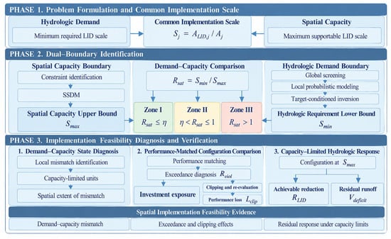
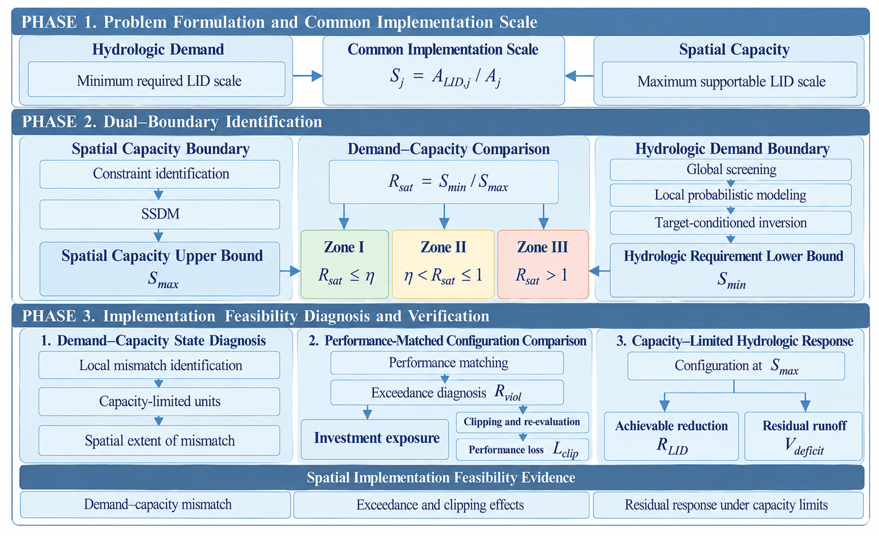
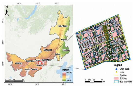
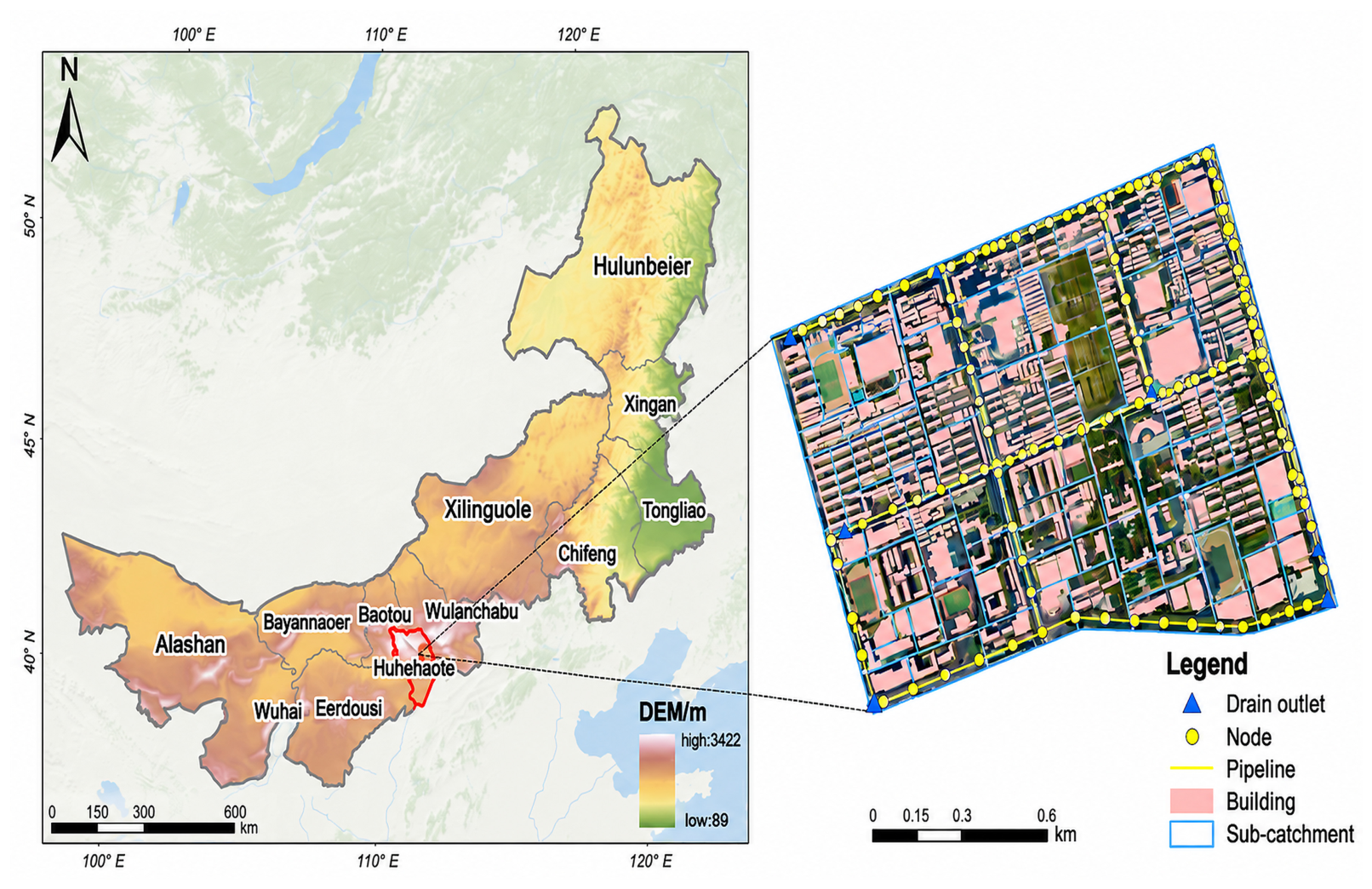
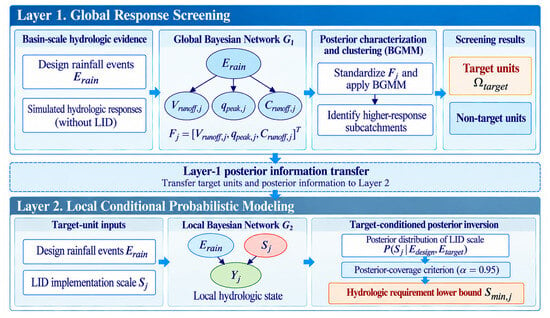
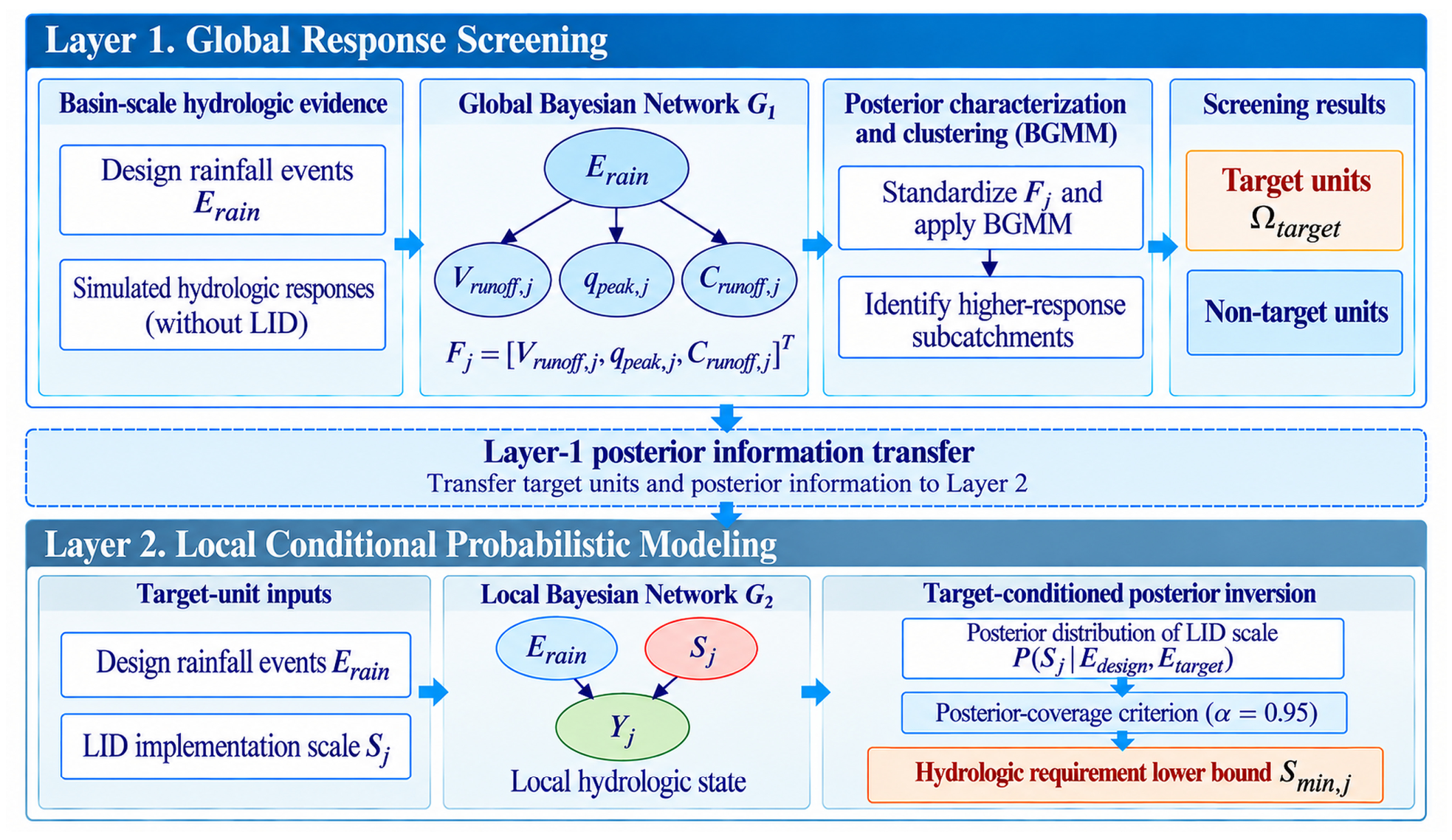
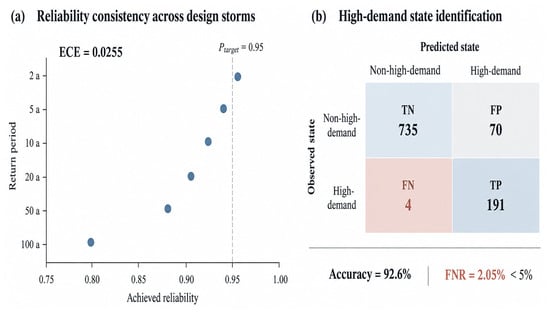
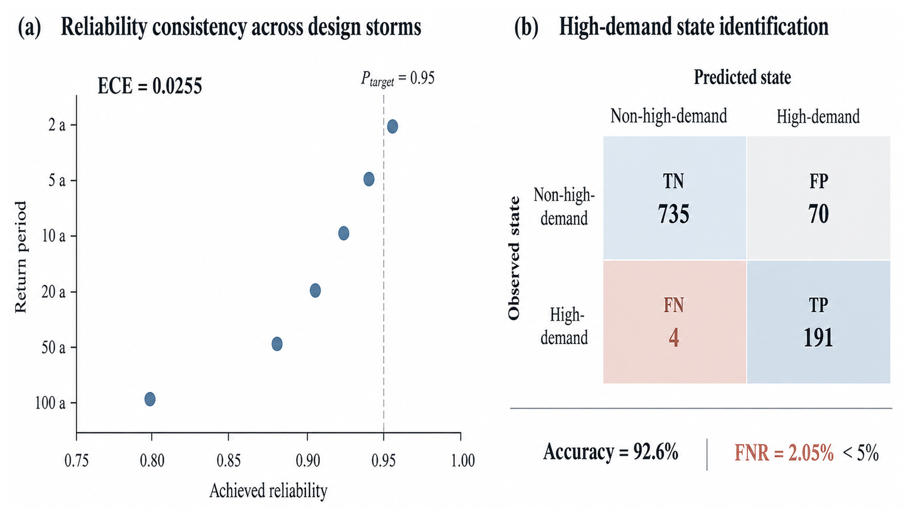
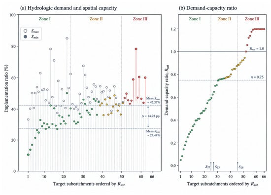
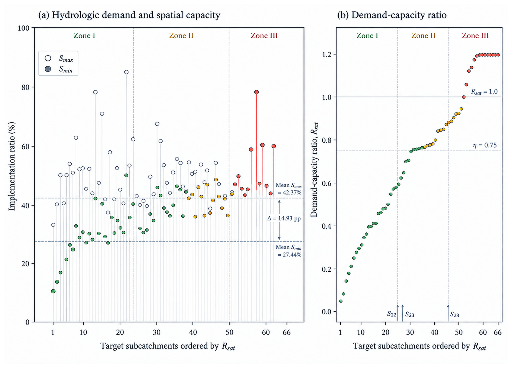
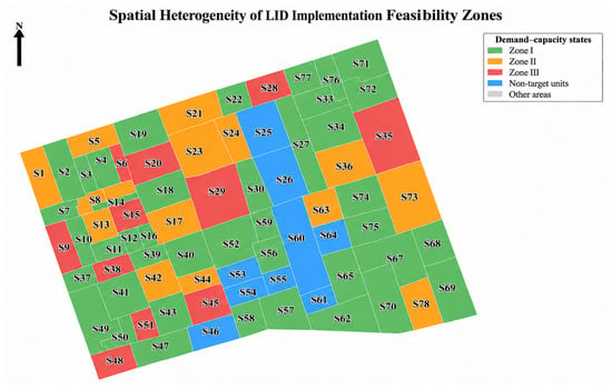
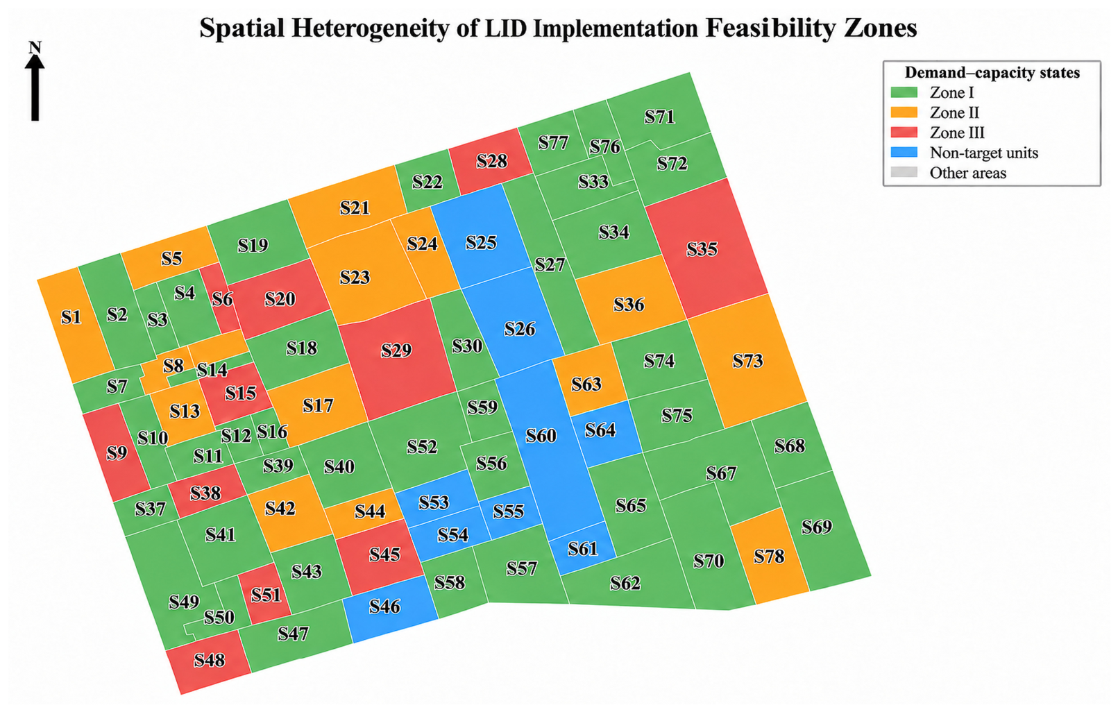
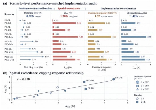
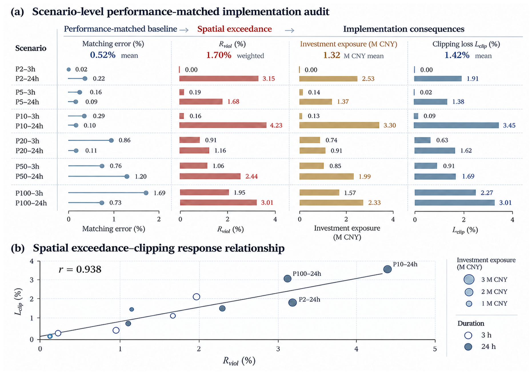
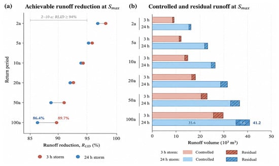
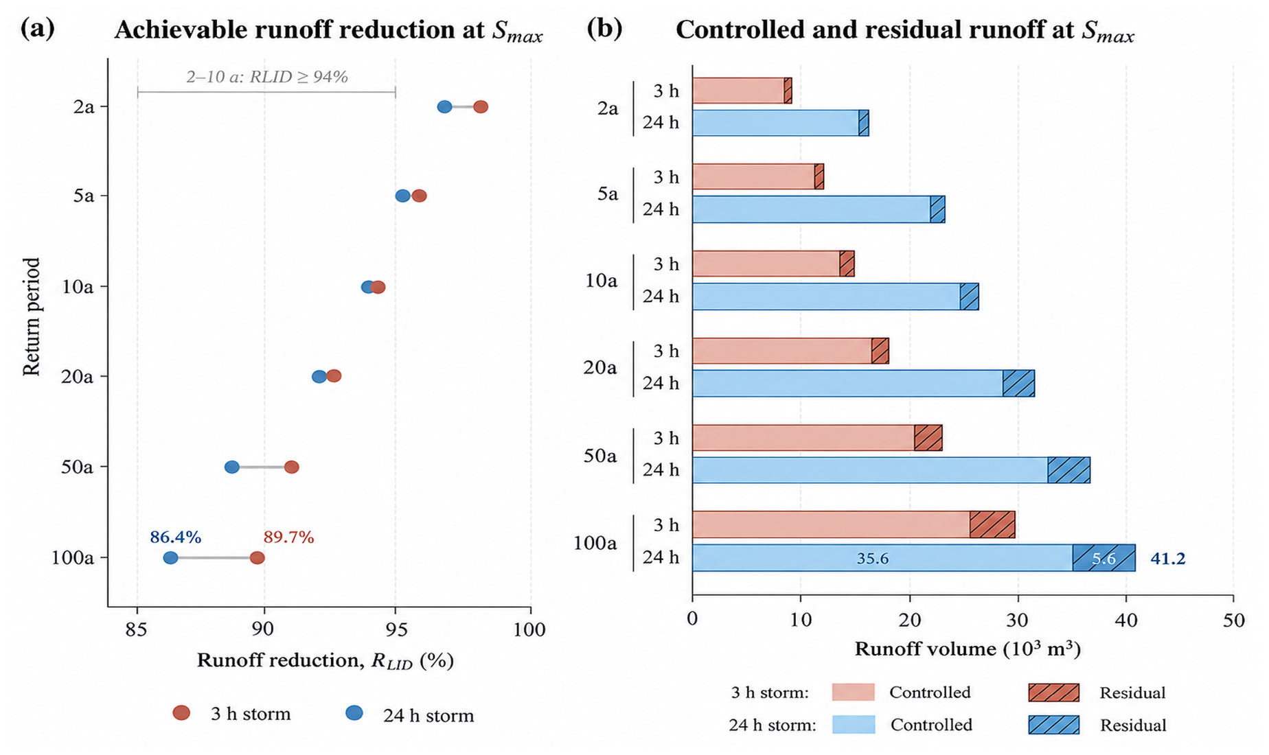

Disclaimer/Publisher’s Note: The statements, opinions and data contained in all publications are solely those of the individual author(s) and contributor(s) and not of MDPI and/or the editor(s). MDPI and/or the editor(s) disclaim responsibility for any injury to people or property resulting from any ideas, methods, instructions or products referred to in the content. |
© 2026 by the authors. Licensee MDPI, Basel, Switzerland. This article is an open access article distributed under the terms and conditions of the Creative Commons Attribution (CC BY) license.