


Abstract
Quantifying rainfall variability is essential for understanding hydroclimatic behavior in vulnerable semiarid regions characterized by strong spatial and temporal variability. This study proposes Math-SPI-Pro as an alternative computational framework for precipitation anomaly standardization assessing drought. The approach retains the conventional gamma/mixed-gamma probabilistic basis used in SPI, including Thom’s approximation for gamma parameter estimation, while applying a direct standardization of the resulting cumulative probability H(x). Consequently, the Math-SPI-Pro standardized scale is mathematically related to, but numerically distinct from, the conventional inverse-normal SPI transformation. The approach incorporates an analytical treatment of the gamma distribution, including the evaluation of scale-dependent changes in the shape of the fitted gamma distribution and the explicit consideration of the precipitation series with and without zero values, enabling a more robust probabilistic representation across the time scales. The method was implemented for spatial–temporal drought characterization in a semiarid basin of Mexico and compared with three commonly SPI models used (SPI_SL_6, Climpact, and Variclim). Results show that the proposed Math-SPI_Pro formulation achieved high agreement with the reference models, with a Pearson correlation coefficient close to 0.98 and generally small pairwise discrepancies according to the error metrics. These findings demonstrate that the proposed analytical framework provides an explicit and reproducible alternative framework for standardized precipitation anomaly for drought assessment for sustainable water management in applications such as reservoirs, aquifers, and surface water; disaster prevention; agriculture; and socioeconomic issues.
1. Introduction
Freshwater availability is strongly influenced by geographic location, climate, topography, vegetation, and the occurrence of drought [1,2]. Drought is a recurrent hydroclimatic phenomenon associated with precipitation deficits [3,4], and its analysis relies on numerical models, geospatial techniques, artificial intelligence, and computational algorithms [5]. Large-scale atmospheric and oceanic processes may also influence precipitation variability [6], contributing to the stochastic behavior of rainfall [7] and to the occurrence of alternating wet and dry periods [8].
Drought characterization commonly considers different factors such as duration, intensity, magnitude, spatial variability, and temporal scale [9]. Different drought types may affect environmental and socioeconomic systems [3,10] and can be evaluated using different hydroclimatic variables [11]. Operational drought tools have traditionally focused on the identification of dry events, although wet periods and their recurrence may also be relevant for hydroclimatic assessment [12,13]. The reliability of these analyses may be limited by data availability [14], which reinforces the importance of long-term observations from meteorological stations for model calibration and validation [15]. Drought-monitoring methodologies have therefore been developed for different regions and precipitation regimes [16,17].
Different drought types respond to different temporal scales. Meteorological drought is generally associated with short precipitation deficits [18] and may also be assessed using refined computational algorithms [19]. Agricultural drought is related to soil moisture deficits and short-term precipitation variability [20], while evapotranspiration and temperature can further affect water availability [21]. Indices such as the Palmer Drought Severity Index have also been used for this purpose, although with recognized limitations [22]. Hydrological drought generally develops over longer accumulation periods and affects streamflow, reservoirs, and groundwater [23], and alternative signal-processing approaches have also been applied to its analysis [24]. Socioeconomic drought can emerge when water availability is insufficient to meet demand [25], whereas ecological drought is associated with alterations in ecosystems and vegetation [26] and can be evaluated using indices such as the Standardized Precipitation Evapotranspiration Index [27]. These different temporal responses highlight the importance of indices that can be consistently evaluated at multiple accumulation scales.
Among these indices, the Standardized Precipitation Index (SPI) [28,29] is widely used for the characterization of wet and dry conditions and is recommended by the World Meteorological Organization [30]. The conventional SPI methodology fits accumulated precipitation to a probability distribution, commonly to the gamma distribution, and subsequently transforms the cumulative probability to the standard normal distribution [31,32]. Although the probabilistic basis of the SPI is well established, its computational implementation can differ among algorithms. In particular, parameter estimation procedures, treatment for zero precipitation, evaluation of the gamma functions, and subsequent numerical transformations are not well-described, hindering verification and reproduction, for example, from a methodological point of view.
This lack of transparency is relevant because different data-processing, parameterization, and numerical-approximation procedures may introduce discrepancies among SPI implementations [9]. Consequently, reproducible computational procedures are needed to reduce methodological uncertainty and facilitate verification of SPI calculations [33]. The main gap addressed in this study is therefore not the definition of a new probabilistic drought model, but the need for a transparent and reproducible computational framework in which the parameter estimation and probability evaluation steps can be explicitly followed and verified. Moreover, the specific treatment for basins under semiarid conditions, or to put it better, with scarce or null precipitation events, was gamma function, which presents certain particularities.
Based on the previous study, the objective of this study is to develop and evaluate Math-SPI-Pro as an alternative computational framework for SPI estimation, addressing limitations associated with restricted transparency in existing implementations of SPI.
The proposed framework retains gamma-based precipitation modeling while explicitly documenting the calculation procedure. Gamma parameters are estimated using Thom’s closed-form approximation to the maximum-likelihood solution, followed by direct evaluation of the gamma probability functions and treatment of zero precipitation through the mixed-gamma formulation. However, Math-SPI-Pro differs from the conventional SPI in the final standardization step, because the mixed-gamma cumulative probability H(x) is standardized directly using its mean and standard deviation rather than being transformed through the inverse standard-normal distribution.
Therefore, Math-SPI-Pro provides a modified standardized representation of the same underlying cumulative probability rather than a numerically equivalent implementation of the conventional SPI. The resulting SPI series are compared with those generated by SPI_SL_6, Variclim, and Climpact using common precipitation datasets from two stations in a semi-arid Mexican basin.
2. Materials and Methods
The analysis presented in this article was conducted using Fortran for daily data and its conversion to monthly precipitation. Mathematica® (v14.0) was used for the analytical computational procedure of the Math-SPI_Pro algorithm, and it was validated using a common database. Its performance was compared with different platforms and software such as Climpact, SPI_SL_6, and Variclim [33,34]. In order to assess the data distribution, the SPI-12 scale was used for all the algorithms with daily climate data from meteorological station databases from 1993 to 2022 in the upper basin of the Aguanaval River in a semi-arid region.
The whole algorithm’s performance was evaluated using statistical metrics, including Pearson’s correlation coefficient (r), mean error (ME), mean absolute error (MAE), and the root mean squared error (RMSE). Because consecutive SPI-12 values are derived from overlapping accumulation windows, inferential tests requiring independent observations were not used for formal hypothesis testing. Spatial and temporal characterization of the study area will provide key information for water resource management and decision-making.
2.1. Description of the Study Area
The hydrological system study is located inside Hydrological Region 36 (Nazas Aguanaval), classified by the National Mexican Water Law for its management and administration, as well as for the development of its hydraulic infrastructure. One of the sub-basins of the upper Aguanaval River is situated in the north-central region of the state of Zacatecas, Mexico, within the municipality of Fresnillo. The catchment area includes the Rio Chico, which flows through the Santa Rosa dam (SR), located at coordinates 22°55′33″ N latitude and 103°06′46″ W longitude, with a capacity of 10.476 Hm3, together with the El Sauz Leobardo Reynoso dam (LR), situated at 23°16′54″ N latitude and 103°06′32″ W longitude, with a maximum capacity of 95.717 Hm3. The region presents a topography composed of high mountains with an average altitude of 2240 m above sea level. According to the Köppen methodology modified by Enriqueta García, the weather classification is temperate semi-arid, situated in a semi-desert environment with a temperate semi-arid climate (BS1kw). The SR reservoir (185.76 km2) and the LR reservoir (1232.96 km2) belong to the Mexican Irrigation District 034. The sub-basin polygon spans an area of 2085.41 km2 (Figure 1).
Figure 1.
Spatial distribution of the study area location.
The study was conducted using precipitation records from two meteorological stations, Santa Rosa (SR) and Leobardo Reynoso (LR), located within the investigated semi-arid basin. These stations provide two site-specific precipitation records for evaluating the different software, such as the Math-SPI_Pro analytical framework. Therefore, the comparison between SR and LR should not be interpreted as a regional spatial validation of Math-SPI_Pro but as a methodology that can be implemented in semi-arid or arid conditions related to scarce or null rainfall events.
In the present work, topographic information from 2010 was obtained from the vector data set digitally edited by INEGI [5]. This dataset comprises shapefiles for the maps f13-b35, f13-b36, f13-b45, f13-b46, f13-b55, f13-b56, f13-b65, and f13-b66 [35].
The maps were geographically referenced in the UTM coordinate system and in the North American Datum of 1984 projection of WGS-1984 UTM ZONE 13N parallels and meridians. The previous was delimited using the ArcGIS® v10.5 geographical information system.
The annual rainfall average is 443 mm; the upper basin of the Aguanaval River collects the runoff at a convergence point well-known as “El Salto” (Figure 1).
From the geological point of view, the region is composed of clastic sediments with the presence of tuffaceous sands and conglomerates, which were deposited in the tectonic basin. According to INEGI [36], the predominant soil type is chernozem, covering approximately 35% of the basin territory with high water and nutrient retention capacity, making it ideal for agricultural production. The SR dam and LR dam are primarily used for irrigated crops [37].
2.2. Tools Assessment
Multiple studies have highlighted the need for methodological adjustments in the calculation and application of the SPI, as well as the need to address the methodological limitations because of the lack of general consensus on the categories used [8,31,38].
The legacy SPI_SL_6.exe executable provided by the National Drought Mitigation Center (NDMC), University of Nebraska–Lincoln, was used in this study [39,40]. SPI_SL_6 is a Windows platform compiled in C++ that estimates SPI from monthly precipitation records using the gamma distribution. For the inter-method comparison, the same monthly precipitation series from 1993 to 2022 were used for both stations, and SPI-12 was selected as the common accumulation scale. This tool tends to overestimate drought based on the SPEI, exhibiting trends of increasing frequency, intensity, magnitude, and duration of droughts [18,41,42]. The frequencies that represent the number of occurrences of an event associated with these indices are not reproducible. Some studies have attempted to apply SPI_SL_6 to other variables, but this requires a strong justification, as its original formulation is based on the rainfall distribution, and recent research continues using this resource in order to evaluate both the SSI-12 (Standardized Streamflow Index-12) [40,42] and the SDI (Streamflow Drought Index), due to its versatility and ability to adapt to different variables [42].
Variclim is a web-based tool developed by the Laboratory of Climate Variability, Remote Sensing and Risk Assessment of the Autonomous University of San Luis Potosí (UASLP), Mexico [34]. The platform was implemented using Apache, PHP, and PostgreSQL. A formal public version identifier for the SPI module is not available in the references consulted; therefore, it was possible to access the web platform with permissions provided by the authors [37] from 5 October 2024. The SPI module was run using the same monthly precipitation records for the SR and LR stations, with the 12-month accumulation scale retained for the common comparison among methods. No independent peer-reviewed validation study or open code for this specific SPI implementation was identified; nevertheless, a comparison of its validation was performed with respect to other software results. This tool only determines the SPI with the disadvantage of not computing periods and frequencies.
On the other hand, Math-SPI_Pro is the algorithm proposed in this research work, and it was developed in Mathematica® v14.1 software [43] to obtain the SPI index. The algorithm details the calculation steps from parameter estimation by using different processes: Thom’s closed-form approximation to the maximum-likelihood solution for gamma parameter estimation, followed by direct evaluation of the gamma probability functions, the mixed-gamma transformation, and final standardization. The data window (frequency) was defined for each time scale and processed in a program developed in Fortran.
Finally, ClimPACT2 v1.3.0 (hereafter Climpact) was used through its station-data GUI implementation developed under the WMO Expert Team on the Sector-Specific Climate Indices (ET-SCI) framework [32]. ClimPACT2 is implemented in R and, in the source-code version used here, the SPI routine applies a gamma distribution with unbiased probability-weighted-moment fitting (fit = “ub-pwm”) and a rectangular accumulation kernel. The implementation provides SPI at 3-, 6-, and 12-month accumulation scales; SPI-12 was retained for the common comparison performed in this study.
2.3. Precipitation Data Collection
The databases of the Mexican Hydrological Information System (https://sih.conagua.gob.mx, accessed on 29 December 2025) contain historical records to the present. These databases include climatic daily data for rainfall, mean, maximum and minimum temperature, and evaporation. Also, water storage expressed in volumes are reported from hydrometric stations. Two specific points were analyzed for assessing the SPI models previously explained in a semiarid Mexican region: Santa Rosa dam (code: STRZC-32053) and El Sauz Leobardo Reynoso dam (code: LREZC-32018), located in Zacatecas, México. For this study, long-term historical precipitation data from the period 1993–2022 (30 years) were analyzed, according to the recommendations of the World Meteorological Organization (WMO) which establishes a minimum period of 30 years to ensure climatological representativeness. This period corresponds to approximately 11,000 daily precipitation records, providing a sufficiently large dataset for robust statistical analysis [44]. The use of an extended database is essential to ensure the reliability of the gamma distribution fitting. A large dataset improves the stability of the estimated parameters and reduces the uncertainty in the probabilistic modelling of precipitation, which is fundamental for accurate SPI computation.
Before SPI calculation, the daily precipitation records from both stations were subjected to quality-control and consistency screening. The chronological records were checked for missing observations and potentially anomalous or physically inconsistent precipitation values. Missing daily precipitation records represented less than 10% of the analyzed series. These missing observations were completed using monthly mean imputation; the corresponding monthly mean precipitation was used to complete missing records before aggregation of the daily data into monthly precipitation totals. Recorded zero-precipitation values were not considered missing data and were preserved as valid observations because they are characteristic of the semiarid precipitation regime and are explicitly accounted for by the mixed-gamma formulation used for SPI estimation.
Potential extreme precipitation values were not automatically removed. They were identified through a quartile-based exploratory screening and checked against the original station records; observations considered valid were retained in the analysis.
The long-term precipitation records of the Santa Rosa and Leobardo Reynoso stations have previously been examined in published regional studies addressing homogeneity, persistence, and temporal changes in precipitation records in Zacatecas. These previous assessments provide useful background information on the statistical behavior of both stations. However, because the present study uses a specific 30-year period (1993–2022), no assumption of complete homogeneity was made only on the basis of those earlier studies. No additional statistical adjustment or artificial homogenization was applied to the precipitation values used here. Consequently, the SPI analysis was performed using the SIH-CONAGUA observational records after the missing-data treatment and quality-control screening described above.
In this research, a quartile-based exploratory screening procedure was applied to the precipitation data in order to identify potential anomalous and extreme observations. The first (Q1) and third (Q3) quartiles were calculated to characterize data dispersion and identify observations located at the extremes of the precipitation distribution. These observations were subsequently checked against the original climatological records rather than being automatically excluded from the dataset. Therefore, this procedure was used as a data-quality screening step and not as a statistical analysis. An algorithm was developed in the Fortran programming language (.f90) to aggregate the daily precipitation records into monthly precipitation totals, as shown in Figure 2.
Figure 2.
Monthly precipitation flowchart from daily values.
To further assess the temporal consistency of the precipitation records, homogeneity was evaluated using the annual precipitation series for the 1993–2022 period (n = 30 years). Four complementary tests were applied: Pettitt, Standard Normal Homogeneity Test (SNHT), Buishand range test, and von Neumann ratio test, using a significance level of α = 0.05 [12,45].
The calculation of the SPI is based on McKee methodology; monthly precipitation is fitted to a probability density function (PDF) with the alpha (shape) and beta (scale) parameters. Subsequently, this distribution is integrated with the cumulative distribution function (CDF) for each accumulated precipitation interval. Additionally, the mixed gamma distribution is incorporated, which assigns the probability to rainfall values, taking into account the presence or absence of zeros in the distribution within a defined time scale. Finally, precipitation is standardized with the mean and standard deviation of the distribution [25,46].
In Math-SPI_Pro, the gamma parameters are estimated from the vector of positive precipitation values using Thom’s approximation to the maximum-likelihood solution [17]; the optimal parameters that govern the transformation were constructed based on a vector of positive precipitation values.
Math-SPI-Pro retains the gamma/mixed-gamma probability modeling stages used in the conventional SPI procedure but differs in its computational implementation and final standardization. Gamma parameters are estimated using Thom’s approximation to the maximum-likelihood solution, and the gamma PDF and CDF are subsequently evaluated directly through their mathematical functions. After obtaining the mixed-gamma cumulative probability H(x), Math-SPI-Pro applies a direct linear standardization based on the mean and standard deviation of the H(x) series. In contrast, the conventional SPI transforms the cumulative probability through the inverse standard-normal cumulative distribution function. Therefore, Math-SPI-Pro should be interpreted as a modified standardized representation of the same underlying cumulative probability rather than as a numerically equivalent implementation of the conventional SPI. A step-by-step procedure was developed and is presented in Figure 3.
Figure 3.
Detailed step-by-step process of the algorithm for calculating SPI-12.
- Step 1: Time scale definition
For the meteorological analysis, the computation of successive moving sums was used to quantify precipitation at different time scales. The time scale corresponds to the accumulation of precipitation over different windows according to Henao et al., (2022) [47]. Using the notation ‘1-’, ‘3-’, ‘6-’, ‘12-’, ‘24-’, ‘36-’ time windows for frequencies 1, 3, 6, 12, 24, and 36 months are represented. This method helps smooth short-term fluctuations and highlight more persistent trends or patterns, is common in studies of droughts and seasonal patterns [48].
A twelve-month time window is described to calculate the accumulated precipitation in consecutive intervals within a historical dataset. The function takes a list of monthly precipitation data as input and returns a list with the sum of precipitation over blocks of twelve consecutive months, as follows:
Input: A list of data containing the monthly precipitation recorded for each month within a specified period.
Process: The function calculates the sum of the precipitation for each set of twelve consecutive months. This is done by applying a twelve-month moving window that shifts one position at a time, summing the corresponding values.
Output: A new list with the accumulated precipitation for each block of twelve consecutive months.
- Step 2: Parameter estimation
The parameters of the two-parameter gamma distribution were estimated from the positive precipitation observations using the closed-form approximation to the maximum-likelihood solution proposed by Thom [49], which has been widely adopted in conventional SPI applications, including the procedure described by Edwards and McKee (1997) [25]. For n′non-zero precipitation observations, the auxiliary statistic A was calculated for n observations [50,51]. The fitted probability density function (gamma) was determined using two calibration parameters: alpha (α) and beta (β).
The gamma shape and scale parameters were estimated as follows:
where
- µ = arithmetic mean;
- n′ = number of non−zero data;
- A = auxiliary variable; and
- xi = precipitation (mm).
These expressions correspond to Thom’s analytical approximation to the maximum-likelihood solution rather than to the exact gamma MLE. In Math-SPI_Pro, Thom’s formulation is retained for parameter estimation to maintain consistency with the conventional SPI methodology, whereas the gamma PDF and CDF are subsequently evaluated directly using their mathematical functions.
This formulation is appropriate for the present application because the two-parameter gamma model is fitted to the positive accumulated precipitation values, while zero-precipitation occurrences are treated separately through the mixed-gamma formulation. Its suitability was additionally evaluated through the Kolmogorov–Smirnov goodness-of-fit test, with an adequate gamma fit obtained at the SPI-12 scale for both stations.
- Step 3: Fitting the distribution
In regions of the world classified as arid and semi-arid climates, rainfall can be absent for days or even months. The application of a normal distribution is not suitable for these datasets evaluated over time, so the corresponding probabilistic model should be adjusted. In scientific reports, the performance of various probabilistic models for fitting precipitation data has been evaluated [8]. Therefore, it is suggested to identify the probabilistic model that better fits the specific data of the study region. Gamma or Pearson Type III distributions are typically used for semi-arid regions [5]. The performance of the gamma distribution was evaluated by applying a goodness-of-fit test (GOF-tests). The Kolmogorov–Smirnov (K-S) fit test was performed to compare the distribution of the empirical data with the proposed gamma theoretical distribution [48].
Starting from a continuous distribution, accumulated precipitation (x) can take any positive value. At each time scale, the accumulated precipitation series was fitted to the two-parameter gamma probability density function (PDF), (g(x)), defined in Equation (4):
- x > 0 positive accumulated precipitation (mm);
- α = shape parameter;
- β = scale parameter;
- t = dummy integration variable used in Equations (5) and (6).
The gamma probability density function is defined as a two-parameter distribution commonly used to represent precipitation totals. The gamma function appears as a normalization constant (Γ(α)), and is defined for α > 0 by Equation (5), where t is a dummy integration variable.
The cumulative probability is obtained by integrating the probability density function (PDF) resulting in the cumulative distribution function (G(x)). G(x) is represented by the incomplete gamma function [21] and is the method adopted by the NDMC [22], as shown in Equation (6):
Gamma parameters were first estimated using Thom’s approximation. The resulting parameters were then used to evaluate the gamma PDF and CDF integral directly in Mathematica® for the different time scales [46,52]. The integral (G(x)) is evaluated for precipitation values different from zero, considering the function for positive precipitation values and calculating the cumulative probability for a specific precipitation interval. Since the gamma function (G(x)) is undefined for x = 0, the precipitation distribution may contain zeros, and the cumulative probability then requires x = 0 and G(x) = 0 to avoid indeterminations.
- Step 4: Mixed Gamma
The mixed gamma distribution incorporates the probability of zero precipitation events. The cumulative probability transformation H(x) is therefore evaluated using Equations (7)–(9), which adjust the cumulative probability at precipitation values equal zero.
where
H(x) = q + p ∗ G(x)
p = 1 − q
- m = months without precipitation;
- n = total amount of data;
- q = probability associated with months without rainfall;
- p = probability that a non-zero precipitation value occurs.
Once the mixed-gamma cumulative probabilities H(xi) are obtained for the complete series, their arithmetic mean μH and standard deviation σH are calculated directly from the H(xi) values, rather than from the original precipitation observations xi. These parameters are subsequently used to standardize the cumulative probability series according to Equation (10).
In Math-SPI-Pro, the mixed-gamma cumulative probability H(xi) is standardized directly using its sample mean and standard deviation. Therefore, the resulting variable represents a bounded standardized cumulative probability score rather than the conventional inverse-normal SPI transformation. This formulation preserves the monotonic ordering and cumulative probability information of the fitted precipitation distribution while using a linear standardized scale. Because H(x) is bounded between q and 1, the resulting standardized score is also bounded. For SPI-12, q = 0 at both stations; consequently, the numerical range differs from that of the conventional SPI, although both representations can be related through their common cumulative probability.
Once the mixed-gamma cumulative probabilities (H(xi)) are obtained for the complete series, their arithmetic mean (H) and sample standard deviation (H) are calculated directly from the cumulative probability values, rather than from the original precipitation observations. The Math-SPI-Pro standardized value is then calculated as follows:
where µH is the arithmetic mean of the transformed cumulative distribution, σH is the standard deviation of the transformed cumulative distribution, Z(xi) is the Standardized Precipitation Index (SPI), N is the number of cumulative probability values, H(xi) represents the mixed-gamma cumulative probability associated with precipitation observation xi.
For complete numerical traceability of the Math-SPI-Pro procedure, the SPI-12 calculation sequences for the SR and LR stations are provided in Appendix E. The tables reported, for each 12-month accumulated precipitation value, the corresponding gamma PDF, gamma CDF, mixed-gamma cumulative probability (H(x)), H(x)-mean, standard deviation of (H(x)), and the resulting SPI-12 value.
This relationship provides a direct mathematical link between the Math-SPI-Pro standardized scale and the conventional SPI scale. Thus, the two representations preserve the same underlying cumulative probability while expressing it on different numerical scales.
2.4. Statistical Analysis
The SPI was evaluated for all the time series but particularly for the 12-month scale SPI-12 series. The Pearson correlation coefficient (r) was used to evaluate the agreement between the SPI series and quantify the relationship between the four selected models at this frequency. Each of these distributions is fitted to every time window of our initial model setup. It explores the trend of the components in the time series for a set of t time data for [ai,bi] [51,53] (Equation (14)). This analysis involves the correlation coefficient for each pair of tools, considering all possible permutations between them. By using all pairwise combinations, it was possible to identify the degree of linear correlation between the different models.
In addition, the mean error (ME), the mean absolute error (MAE), and the root mean squared error (RMSE) were computed as Equations (14)–(16), respectively. The typical error of the different SPI calculation algorithms was estimated through a pairwise comparison, where the SPI values obtained using Math-SPI_Pro were evaluated against those derived from SPI_SL_6, Variclim, and Climpact, respectively. This approach allowed for a direct assessment of the discrepancies between methods, providing a consistent framework to quantify the magnitude of error associated with each algorithm. Thus, the pairwise numerical discrepancies and consistency among the outputs of the evaluated methods are quantified. In order to estimate the typical error of the different SPI calculation algorithms, the following metrics were used:
- r = a real number range [−1, 1];
- = corresponds to the average value of the observational estimates over the entire analyzed period;
- ai, bi = are the true data sets;
- i, represent the number of each data set, from 1 to t.
- n = total number of paired SPI values;
- zi = reference SPI value for observation i;
- SPI value obtained with the method being compared at observation i.
Because Math-SPI-Pro applies a bounded standardization of the mixed-gamma cumulative probability, whereas the conventional implementations use the inverse-normal transformation, ME, MAE, and RMSE were interpreted as descriptive measures of numerical discrepancy rather than as absolute measures of predictive error.
Because the SPI-12 series are constructed from overlapping precipitation accumulation windows, consecutive observations are not statistically independent. Therefore, inferential tests that assume independent observations were not used for formal hypothesis testing. The comparison among SPI computation methods was instead based on descriptive agreement and discrepancy measures, including Pearson’s correlation coefficient, ME, MAE, and RMSE, together with the temporal comparison of the resulting SPI series. These metrics were interpreted as comparative measures among methods rather than as independent-sample inferential tests.
No single SPI method was considered a reference or ground-truth method. Pearson’s correlation coefficient, ME, MAE, and RMSE were calculated pairwise between the SPI-12 series generated by SPI_SL_6, Variclim, Math-SPI_Pro, and Climpact. Therefore, these metrics quantify numerical agreement or discrepancy between each pair of computational methods rather than accuracy relative to an external reference.
To provide a method-independent comparison of drought-event identification, a common post-processing criterion was applied to the SPI-12 series generated by SPI_SL_6, Variclim, Math-SPI-Pro, and Climpact. A drought event was defined as a continuous period of negative SPI values that reached SPI ≤ −1.0 at least once and ended when SPI returned to a non-negative value. Event severity was classified according to the minimum SPI reached during each event as moderate (−1.00 to −1.49), severe (−1.50 to −1.99), or extreme (≤−2.00). For each event, onset, termination, duration, minimum SPI, and the date of the minimum were determined. The same criterion was applied to both stations and all four methods as a post-processing procedure of the resulting SPI-12 series.
3. Results and Discussion
Monthly precipitation totals were fitted to a two-parameter gamma distribution. The cumulative probability was obtained through the incomplete gamma function. Because the precipitation records may include zero values, the cumulative probability was adjusted using a mixed distribution where the probability of zero precipitation was explicitly incorporated. It is necessary to establish a general consensus on the calculation steps of the SPI for the detection and projection of precipitation anomalies in order to reduce the uncertainty caused by the multiple calculation possibilities [8]. The analysis in this study focuses on evaluating the Math-SPI_Pro analytical procedure, which includes four main steps described in an algorithm that outlines the tasks required to determine the SPI at multiple scales. This work is applied to precipitation data from two stations, Santa Rosa (SR) and Leobardo Reynoso (LR), located within the investigated semi-arid basin in Mexico. The analysis examines the precipitation distributions and the resulting SPI values at different time scales, allowing the analytical procedure to be evaluated under contrasting precipitation conditions within the study area. The corresponding station data and methodological details are provided in Appendices A and B, while the Math-SPI_Pro algorithm is presented in Appendix C, drought events and the table summary are presented in Appendix D, and, finally, the SR and LR complete numerical sequence for the 12-month scale are provided in Appendix E.
Table Appendix D provides the complete SPI-12 drought-event characterization for the Santa Rosa (SR) and Leobardo Reynoso (LR) stations using the four estimation methods (1993–2022).
By requiring fewer steps, the proposed model could be more accurate, as the simplification of the process helps reduce uncertainty. Evaluating the same dataset, SPI-12 was analyzed, obtaining four consistent distribution patterns through the use of multiple tools.
3.1. Model Performance
The spatial-temporal analysis was conducted using daily precipitation data converted to monthly precipitation, covering the period from 1993 to 2022, where different temporal scales can be selected.
SPI-12 was used as a common accumulation scale to evaluate temporal agreement and numerical discrepancies between Math-SPI-Pro and the other computational implementations. Because Math-SPI-Pro and the conventional SPI implementations use different final standardization scales, the comparison was intended to evaluate consistency in temporal behavior and differences in numerical magnitude rather than to establish absolute predictive accuracy. Despite the widespread adoption of SPI in multiple studies, few describe the step-by-step data processing in detail [54], highlighting the importance of this methodological review.
Additionally, Mathematica® and ArcGIS® were key tools in compiling and executing the spatial temporal analysis, demonstrating their versatility for evaluating and modeling wetter and drier events at different temporal and spatial scales.
Math-SPI-Pro preserves the temporal pattern of precipitation anomalies while producing smaller numerical extremes as a consequence of its bounded standardization. Therefore, differences in magnitude relative to the other implementations should not be interpreted directly as overestimation or underestimation but as differences associated with the final standardization scale, which impacts the global identification of droughts and excess moisture. Furthermore, the algorithm can potentially be applied to other regions and climate types, although additional validation with independent datasets is required, making it a versatile tool for the analysis of hydrometeorological events.
The previously mentioned statistical tests were analyzed in combination with four tools: SPI_SL_6, Variclim, Math-SPI_Pro, and Climpact. These tools were used to evaluate the performance of SPI estimation using the same climatological database corresponding to the SR and LR stations for 1-, 3-, 6-, 9-, 12-, 24-, 36-, and 48-month precipitation scales. The results are presented in detail, and differences were observed.
Additionally, the analysis was not limited to numerical evaluation but also incorporated a spatiotemporal study. This study integrated historical data and variations in precipitation patterns at the stations, allowing for the identification of how these tools represented precipitation anomalies within a regional context. This approach assessed their ability to model climatic phenomena such as drought across different locations and temporal scales.
3.2. Precipitation Data Preprocessing
A program was developed in Fortran for data reading and the calculation of daily precipitation sums over a 30-year period, including leap year days. This subroutine generates the monthly precipitation. Consequently, no monthly precipitation observations were discarded. For example, the maximum monthly precipitation of 323.83 mm recorded at the SR station in July 2002 was retained as a valid extreme precipitation event. Zero-precipitation values were also retained in the original series and were subsequently treated explicitly through the mixed-gamma formulation used for SPI estimation.
After the different homogeneity tests, none of the four tests rejected the null hypothesis of homogeneity for either SR or LR (p > 0.05). Therefore, no statistical homogenization or adjustment of the precipitation series was required before SPI calculation (Table 1) [15].
Table 1.
Homogeneity tests applied to annual precipitation records (1993–2022).
From the previous Table 1 it is possible to mention that precipitation series is homogeneous at an alpha = 0.05, so Ho was not rejected for either station in any of the four tests.
An absolute frequency histogram was used to visualize the graphical representation of the climatological data sample through a continuous frequency distribution. It is recommended to carefully review the behavior of precipitation databases in each region.
The goodness-of-fit (GOF) of the two-parameter gamma distribution was evaluated using the Kolmogorov–Smirnov (Dks) test independently for each accumulation scale and station (Table 2). The test was applied to the positive accumulated precipitation values used for gamma parameter estimation, while zero-precipitation occurrences were treated separately through the mixed-gamma formulation. The results show that the goodness-of-fit is scale-dependent. At a significance level of α = 0.05, the null hypothesis of consistency with the fitted gamma distribution was not rejected for the 3-, 9-, and 12-month scales at the SR station and for the 1-, 3-, 9-, 12-, 36-, and 48-month scales at the LR station. Particularly, at the SPI-12 scale used for the main inter-method comparison, the gamma distribution showed an adequate fit at both stations: SR Dks = 0.0659|p = 0.0922; LR Dks = 0.0553|p = 0.2276.
Table 2.
Gamma distribution parameters and Kolmogorov–Smirnov goodness-of-fit results for different precipitation accumulation scales.
In Table 2, n+ denotes the number of positive accumulated precipitation values used for fitting the continuous two-parameter gamma distribution. Dks is the one-sample Kolmogorov–Smirnov statistic. Zero-precipitation occurrences were treated separately through the mixed-gamma formulation. Gamma parameters were estimated from the same data using Thom’s approximation to the maximum-likelihood solution; therefore, the reported p-values are conventional K–S p-values and should be interpreted as approximate goodness-of-fit diagnostics rather than exact inferential probabilities. In the same sense H0 indicates that the positive accumulated precipitation values are consistent with the fitted two-parameter gamma distribution. At α = 0.05, H0 is not rejected when p > 0.05. Gamma parameters were estimated using Thom’s approximation to the maximum-likelihood solution.
These results indicate that the suitability of the gamma model varies with temporal aggregation and should therefore be evaluated for each accumulation scale.
The GOF tests can fit different probability distributions depending on the study region. The change in a variable other than precipitation does not always follow a gamma distribution. This could significantly affect the results and, consequently, the calculation of the SPI. It is the responsibility of the researcher to mitigate any bias that may increase uncertainty in the results.
Histograms facilitate the graphical representation of the distribution. Initially, for SPI-3, the distribution presents an inverted “J” curve shape (type A), due to the frequency of zeros occurring in the dataset. As the time scale increases, the distribution of the data becomes more symmetrical and approaches a gamma normal distribution curve. In SPI-12, the zeros were eliminated because it is uncommon for there to be no rainfall over 12 months, as shown in Figure 4 (type B). The horizontal axis represents the precipitation intervals (mm) for the SR and LR stations, respectively.
Figure 4.
Comparison of time scales using precipitation histogram for SPI-3 and SPI-12.
- Step 1: Comparison of different time scales
Figure 5 shows the precipitation density modeling for the SR (Figure 5a) and LR (Figure 5b) stations, revealing a particular behavior due to the decrease in zeros in the datasets as the time scale expands. This change is reflected in the tendency of precipitation data to cluster more uniformly around a central value as the temporal scale increases.
Figure 5.
Scale-dependent gamma density curves for SR (a), LR (b), and temporal evolution of SPI patterns (c).
The scale defines a new accumulation vector, calculated at intervals of 1, 3, 6, 9, 12, 24, 36, and 48 months, as shown in Figure 5c. As a result, a new trend and visualization of a pattern defined by time windows can be observed.
Figure 5 illustrates the scale-dependent evolution of the fitted gamma density functions for the SR and LR stations. At shorter accumulation periods, the precipitation distributions are strongly right-skewed and may exhibit a monotonically decreasing or J-shaped density, reflecting the high frequency of low precipitation totals and zero-precipitation occurrences. As the accumulation scale increases, the summation of precipitation progressively reduces the relative occurrence of zero and very low values, and the fitted distributions develop a single interior mode. Consequently, the gamma density evolves from a strongly skewed configuration at short time scales toward a more clearly unimodal distribution at longer accumulation periods. This behavior is observed at both SR and LR stations and reflects the effect of temporal aggregation on the statistical distribution of precipitation.
- Step 2: Key modeling parameters
Table 3 presents a list of essential parameters used in modelling the SPI-12 for the stations SR and LR, over a 12-month period (SPI-12).
Table 3.
Parameters used in the SPI calculation.
The parameters reported in Table 3 correspond specifically to the Math-SPI-Pro calculation at the 12-month scale and should not be interpreted as the parameters used internally by SPI_SL_6, Variclim, or Climpact. Because q = 0 at SPI-12 for both stations, the mixed cumulative probability is bounded by 0 ≤ H(x) ≤ 1. Therefore, the Math-SPI-Pro standardization ZM = [H(x) − μH]/σH gives approximate theoretical ranges of −1.686 to 1.709 for SR and −1.702 to 1.670 for LR. The extreme SPI values among models will be discussed in Section 3.2; however, they confirm numerical consistency between the model parameters and the resulting standardized series.
- Step 3: Gamma fitting
Figure 6a presents a comparative distribution of precipitation values recorded at the two stations, with intervals measured in millimeters (mm) on a 12-month timescale. The spatiotemporal characterization shows differences between the SR and LR stations due to precipitation variability.
Figure 6.
Comparative analysis of the SPI_SL_6 software and the Math-SPI_Pro algorithm. (a) probability density function for both dams (LR-line blue and SR dam in red color), (b) Math SPI model performance with 12 window frequency for both dams SR and LR and historical comparison of SPI_SL_6 and Math SPI_Pro for both dams SR (c) and LR (d).
The 12-month accumulated precipitation was higher at the SR station than at the LR station. The mean accumulated precipitation was 474.15 mm for SR and 423.72 mm for LR, corresponding to an approximately 11.9% higher mean at SR. Similarly, the median values were 472.58 mm and 411.61 mm for SR and LR, respectively. The fitted gamma distributions also showed a displacement in their central location, with modal values of 428.43 mm for SR and 386.63 mm for LR, indicating that the LR distribution was shifted by approximately 41.8 mm toward lower accumulated precipitation values. The maximum 12-month accumulation was 976.95 mm at SR and 719.20 mm at LR. Precipitation exhibits different behavior at each station, with limitations in its measurement due to the point-based nature of the stations, which prevents capturing the entire rainfall area in the basin, as shown in Figure 6b.
The SPI data reflects historical precipitation trends, while Math-SPI_Pro results were obtained using the explicit computational procedure described above and were compared with the SPI_SL_6 results. Magnitude and timing of drought events highlight how each method responds to changes in precipitation patterns.
Figure 6c,d presents a comparative analysis between the SR and LR stations. The x-axis represents the temporal scale in months, while the y-axis shows the corresponding SPI-12 index values.
- Step 4: Cumulative probability transformation to Gamma probabilities
The values of p and q were obtained to determine the probability of finding a zero in the data distribution and to apply the mixed gamma model. These values were analyzed for SPI-12, and the key modeling parameters (m = 0, q = 0, p = 1) were obtained for both SR and LR. The comparison revealed that the indices at the SR station reached higher maximums than those at the LR station during the first decade. Conversely, at the LR station, extreme drought events were more severe compared to the second and third decades of the analysis. Overall, the patterns exhibit similar trends and characteristics to the Math-SPI_Pro algorithm.
3.3. Statistical Analysis Between Groups
The series correlated in all possible pairwise combinations, and the behavior of the dry and wet cycles was clearly defined. This analysis was carried out using SPI-12 in different regions of the SR and LR stations, as shown in Figure 7.
Figure 7.
Comparison of SPI-12 values: (a) Pearson correlation, (b) ME, (c) MAE, and (d) RMSE.
The SPI values show strong correlations, as indicated by Pearson’s correlation coefficient, which measures the degree of covariance between related variables.
The Pearson correlation matrix, using a color scale, highlights the correspondence between the tools used to calculate the SPI. Figure 7a (SR_SPI-12) shows the strongest correlation, represented in crimson, between SPI_SL_6 and Climpact, followed by a strong correlation between Math-SPI_Pro and Variclim within the same color scale. Figure 7a (LR_SPI-12) presents a color scale consistent with the observed correlation levels. On the other hand, the blue scale indicates the degree of correlation between SPI_SL_6 and Math-SPI_Pro, while the weakest correlation is observed between Climpact and Math-SPI_Pro. Since the absolute value of r is high, the correlation is considered strong, indicating that the variables are strongly related.
The high Pearson correlation coefficients indicate strong temporal agreement among the evaluated series, particularly in the timing and direction of dry and wet anomalies. However, Math-SPI-Pro applies a bounded linear standardization of the mixed-gamma cumulative probability, whereas the compared implementations may express the same probabilistic information on different numerical scales. Consequently, ME, MAE, and RMSE were interpreted as descriptive measures of pairwise numerical discrepancy rather than as absolute measures of predictive error. Thus, a strong correlation can coexist with differences in MAE and RMSE because the temporal patterns may remain similar while the numerical amplitudes differ among methods.
The ME results in Figure 7b suggest, by comparing the values, that Math-SPI_Pro and Variclim exhibit the smallest mean numerical discrepancy compared to SPI_SL_6, indicating small differences between the two methods. This consistency suggests that these methods have very similar behavior in how they model drought, thereby generating comparable SPI values. Climpact exhibits greater variability and tends to differ more from the other three estimation methods, which could suggest a tendency toward overestimation. In contrast, the SPI_SL_6 results obtained with Climpact indicate possible differences in its calculation methodology or the parameters used.
In general, based on the ME analysis, there are no extremely large discrepancies between the evaluated methodologies, and the ME is consistent for the SR and LR stations. However, there are variations that should be considered when selecting a method for the analysis of precipitation anomalies. ME is sensitive to extreme values and can indicate systematic biases, suggesting whether the values are overestimated or underestimated.
In MAE, the average of the absolute differences is calculated, where the differences do not cancel out, allowing for the assessment of general accuracy. The MAE evaluation matrix shows the differences between the various estimation methods, reveals variations in magnitude, and allows for the identification of methods with higher concordance Figure 7c.
The results of the analysis indicate that Climpact exhibits the lowest MAE relative to SPI_SL_6, indicating the closest numerical agreement between these two series among the evaluated comparisons. Regarding alternative method comparisons, Math-SPI_Pro and Variclim also show a high degree of similarity.
The highest error is observed between Climpact and Math-SPI_Pro, highlighting discrepancies. This suggested the use of significantly different approaches to estimate the SPI. Variclim is relatively close to SPI_SL_6 in terms of SPI value estimation, indicating a moderate difference. Although there is some variability between the two, the difference is not excessive. Climpact behaves somewhat differently from Variclim, but the differences are not completely distinct.
The MAE between Math-SPI_Pro and SPI_SL_6 is higher, indicating a greater difference from SPI_SL_6 compared to Variclim. This suggests that Math-SPI_Pro exhibits different behavior with respect to SPI_SL_6, which could reflect a distinct methodology for SPI estimation.
In Figure 7d, the RMSE matrix allows for identifying the magnitude of errors among the SPI-12 values. The highest values, represented in dark tones, are found between Math-SPI_Pro and SPI_SL_6, as well as between Math-SPI_Pro and Climpact, and in the comparison between Variclim and Climpact and Variclim and SPI_SL_6.
In contrast, the lowest values, represented in light tones, correspond to Math-SPI_Pro and Variclim and SPI_SL_6 and Climpact, indicating that these model pairs exhibit greater similarity in their estimations, demonstrating consistency between the results of the stations.
Lower RMSE values indicate smaller numerical discrepancies between pairs of SPI computation methods. In particular, Math-SPI_Pro and Variclim show relatively small pairwise differences, while SPI_SL_6 and Climpact also produce similar SPI estimates. These results are interpreted as evidence of numerical agreement between methods rather than as a measure of absolute accuracy, because no method was defined as a ground-truth reference.
The exact numerical values corresponding to the Pearson correlation, ME, MAE, and RMSE matrices are shown in Figure 7 and are provided in Table 4 for both the SR and LR stations as follows:
Table 4.
Pairwise numerical comparison of SPI-12 values obtained with the four computational methods for the Santa Rosa (SR) and Leobardo Reynoso (LR) stations.
In Table 4, Pearson’s correlation coefficient (r), mean error (ME), mean absolute error (MAE), and root mean squared error (RMSE) were calculated pairwise using the SPI-12 series generated by each method. For the pairwise comparisons reported in this table, ME is expressed as the first method minus the second method; therefore, its sign indicates the direction of the mean numerical difference. MAE and RMSE are non-directional measures of the magnitude of pairwise numerical discrepancy. No method was considered a ground-truth or absolute reference method.
The exact numerical values corresponding to the Pearson correlation, ME, MAE, and RMSE matrices are shown in Figure 7 and are reported in Appendix E for both stations, allowing direct verification of the pairwise comparisons among the four SPI computation methods.
3.4. SPI Model Comparison
As part of the analysis and performance evaluation of the methods, a comparison was made regarding differences in intensity, magnitude, and duration of drought classifications [26]. Intensity, defined as the extreme SPI-12 values, revealed discrepancies across the four tools used, as shown in Figure 8, particularly at the SR and LR stations.
Figure 8.
Comparison of SPI-12 Indices from the four methods for the SR and LR stations. Red and blue colors indicate values below or greater than zero according with its magnitude, respectively. Historical SPI performance per month and models for (a) Santa Rosa Dam and (b) Leobardo Reynoso Dam. Maximum and minimum values are pointed out in each case.
To complement the comparison of individual SPI-12 extremes shown in Figure 8, the four SPI-12 series were evaluated using the common drought-event criterion described in the methodology. This analysis allows the methods to be compared in terms of event onset, termination, duration, minimum SPI magnitude, and severity. The principal drought events are summarized in Table 5, while the complete event inventory for 1993–2022 is provided in Appendix E.
Table 5.
SPI-12 drought-event classification obtained using a common post-processing criterion.
At the SR station (Figure 8a), the peak of the SPI-12 index occurs in month 121, corresponding to extreme wetness in January 2003, for both the SPI_SL_6 and Climpact indices (2.69 and 2.56, respectively). This period is identified as the wettest, characterized by extraordinary rainfall events. In contrast, the Math-SPI_Pro and Variclim indices showing more moderate values (1.70 and 1.87, respectively), reaching their maximum values in month 126, corresponding to June of the same year. It is important to note that extraordinary rainfall events had already occurred in July 2002, reflected in high positive values across all indices, indicating consistency among the different databases used.
The minimum index value is recorded in month 223, corresponding to July 2011, indicating drought conditions. In this case, all four drought assessment tools are in agreement, recording the most critical negative values during this period shown in Figure 8a.
The minimum values show less variability: SPI_SL_6 and Climpact both report a value of −2.24, classified as extreme drought, while Variclim (−1.92) and Math-SPI_Pro (−1.66) reflect severe drought conditions. The categories do not match the between-methods for the same classification, revealing discrepancies in the intensity, magnitude, and duration assigned to the event depending on the tool used.
Differences in maximum values are smaller, with less variation among methods. At the LR station, the maximum SPI-12 values are first identified by the Math-SPI_Pro and Variclim methods, reporting very wet values (1.60 and 1.70, respectively) in month 306 (June 2018), while for SPI_SL_6 and Climpact, which present the highest values (1.99 and 1.93, respectively), they reach their maximum in month 311 (November 2018), as shown in Figure 8b.
For Figure 8b, negative values tend to show greater differences between methods. Regarding extreme drought events at the LR station, they are observed in month 224 (August 2011) for SPI_SL_6 with a minimum of (−2.97), while Climpact records the lowest minimum (−3.03) values classified as extreme drought. In month 225, corresponding to September 2011, Math-SPI_Pro presents the least severe drought intensity (−1.69), and Variclim presents a minimum of (−1.98); both were classified under the same category: severe drought.
The common drought-event analysis showed substantial agreement in the temporal identification of the principal drought episodes, despite differences in SPI magnitude among the four methods (Table 5). At SR, all methods identified their minimum SPI in July 2011. SPI_SL_6 and Climpact classified this minimum as extreme drought (−2.240 and −2.241, respectively), whereas Variclim and Math-SPI-Pro classified it as severe drought (−1.918 and −1.664, respectively). At LR, SPI_SL_6 and Climpact identified the minimum in August 2011 (−2.970 and −3.030, respectively), while Variclim and Math-SPI-Pro identified their minima one month later, in September 2011 (−1.985 and −1.694, respectively). Thus, the methods consistently identified the major 2011 drought episode, while differences in SPI magnitude affected the assigned drought-intensity category.
The accumulation of zeros in precipitation data can affect the parameterization of the adjusted distributions, generating biases in the negative SPI values. This is particularly relevant in arid or semi-arid climates, where dry periods are frequent. Methods such as SPI_SL_6 and Climpact may handle the probability of SPI conversion differently, influencing the magnitude of extreme values.
The different distributions exhibited similar patterns in their temporal variations. Although differences in the magnitude of extreme values were identified, the four methods followed comparable trends, suggesting that each applies a distinct approach to the parameterization and fitting of the distributions.
These findings highlight the ability of the applied methodologies to detect and characterize the spatial and temporal variability of drought, as well as their consistency with observational records available in the evaluated datasets.
Overall, all methods are capable of consistently capturing both drought and wet periods throughout the analyzed time series.
It should be noted that the extreme values of +2.69 and −2.97 reported in Figure 8 were generated by SPI_SL_6, whereas −3.03 was generated by Climpact. These values are therefore not derived from the Math-SPI-Pro parameters reported in Table 5. In contrast, the Math-SPI-Pro extremes (+1.70 and −1.66 for SR, and +1.60 and −1.69 for LR) are consistent with the bounded standardized ranges resulting from the corresponding μH and σH values.
3.5. Comparison of SPI-12 Distributions Among the Different Months
The data distributions were separated and analyzed by month in order to observe the comparison between the different monthly asymmetries (Figure 9). The SPI-12 distribution comparison across both stations highlights the variability and central tendencies among the groups. The figure emphasizes the differences in dispersion, medians, and outliers for each station, providing insight into the spatial patterns of drought intensity. LR shows a concentrated dispersion around the origin (0). This indicates that the data are very close to that value. SR presents greater dispersion, as the median is farther from the origin. This implies that the data in SR are more spread out over a wider range.
Figure 9.
Box plot representation of annual SPI-12 indexes for SR and LR. Negative values of SPI appear as −0.3, −0.6, −0.9, −1.2, −1.5 and −1.8 in the vertical axis in all subfigures.
It is observed that some ranges are wider than others, indicating variability in the ability of the Math-SPI_Pro tool to capture fluctuations in the SPI-12 across different contexts. The box plot presents the distributions of SPI-12 values for different ranges. Wider ranges suggest greater dispersion in the data, which may be related to the sensitivity of each method in identifying extreme precipitation events.
This result is relevant, as it shows that, despite being located within the same sub-basin and only 47 km apart, the SPI-12 series from the LR and SR stations show differences in their temporal patterns, dispersion, and extreme values. These differences are interpreted descriptively because consecutive SPI-12 observations are temporally dependent as a consequence of the overlapping 12-month accumulation windows.
The drought reached its maximum values, mostly in the LR dam. The highest frequency of droughts peaked in June and July, while in December, a peak was observed in SR under the SPI-12 time scale. The months of greatest drought intensity indicate that the region is affected, impacting agriculture, society, and industry. The spatial comparison between interdecadal and interannual periods should be made with caution, as they affect different systems and the data distributions are not the same due to the different aggregation sets [23]. Therefore, it is suggested that comparisons be made within the same aggregation period to ensure proper data management.
Several recent studies have proposed probabilistic approaches for drought characterization using gamma mixture distribution models and Bayesian inference techniques [55]. These methods allow the representation of multiple precipitation regimes and explicitly account for the uncertainty associated with parameter estimation in drought classification. The objective of the present study is not to replace the gamma/mixed-gamma probabilistic basis used for precipitation modeling in SPI, but to provide an explicit computational framework with a modified final standardization of the cumulative probability.
The results demonstrated that the analytical approach produces consistent trends, reducing dependence on numerical approximation procedures during the subsequent probability-evaluation steps. The research focuses on simplifying the SPI calculation and providing a more explicit computational alternative. An important aspect of the comparison is the numerical scale resulting from the Math-SPI-Pro transformation. Because the mixed-gamma cumulative probability H(x) is bounded, its direct standardization using μH and σH also produces a bounded standardized variable. This differs numerically from the conventional inverse-normal transformation, which is unbounded. Nevertheless, the Math-SPI-Pro transformation is monotonic and reversible, since H(x) = μH + σHZM. Therefore, the corresponding conventional SPI value can be expressed as SPIconv = Φ−1(μH + σHZM). This relationship explains why Math-SPI-Pro can preserve the temporal ordering and probabilistic information of precipitation anomalies while producing smaller numerical extremes. Accordingly, the high Pearson correlations mainly reflect similarity in temporal behavior, whereas ME, MAE, and RMSE describe differences in numerical magnitude between the outputs.
From a computational perspective, Math-SPI_Pro differs from the evaluated SPI implementations mainly in the transparency and structure of its calculation procedure. The proposed framework retains Thom’s closed-form approximation for gamma parameter estimation and subsequently evaluates the gamma PDF and CDF directly through their mathematical functions, reducing the number of intermediate approximation steps required during probability evaluation. This provides a numerically stable and reproducible workflow, particularly because each transformation from accumulated precipitation to the final standardized SPI value is explicitly defined. In contrast, the compared tools differ in implementation environment and in the degree to which their internal computational procedures can be inspected or reproduced. Therefore, the present comparison of computational cost is qualitative rather than based on execution-time benchmarks, since SPI_SL_6, Variclim, Climpact, and Math-SPI_Pro operate on different software platforms and architectures. Within this limitation, Math-SPI_Pro reduces procedural complexity while maintaining results comparable to the evaluated SPI tools, and its explicit formulation facilitates replication, verification, and modification of the calculation procedure.
The agreement observed between Math-SPI_Pro and the other SPI tools is restricted to the two meteorological stations and the 1993–2022 precipitation records analyzed in this study; therefore, these results should not be extrapolated to other regions or climate types without validation using additional independent datasets.
4. Conclusions
The objective was to optimize the theoretical method with an analytical approach for the identification of precipitation anomalies, leveraging precise daily rainfall data. The detailed Pearson analysis confirms a strong correspondence between the SPI values obtained in a spatial context, as shown for the SR and LR stations, validating that Math-SPI_Pro provides an explicit and reproducible framework for SPI computation, using Thom’s approximation for gamma parameter estimation followed by direct evaluation of the gamma probability functions. Both methods demonstrate consistency in ME patterns, highlighting their ability to capture temporal variations across different hydroclimatic contexts.
The comparison showed strong temporal agreement among the evaluated SPI series, as indicated by the Pearson correlation coefficients. ME, MAE, and RMSE identified differences in numerical magnitude among the methods and were therefore interpreted as descriptive discrepancy measures rather than as absolute measures of predictive accuracy. The bounded standardization used by Math-SPI-Pro explains part of these magnitude differences while preserving the temporal ordering of precipitation anomalies. Thus, Math-SPI-Pro provides an explicit and reproducible standardized representation of the mixed-gamma cumulative probability that is mathematically related to, although numerically distinct from, the conventional inverse-normal SPI scale. The comparative analysis based on the Pearson correlation, ME, MAE, and RMSE showed that the SPI series generated by the four methods generally followed similar temporal patterns, although differences in the magnitude of individual SPI values were observed. These measures were used to characterize agreement and discrepancies among the computational methods without assuming temporal independence of consecutive SPI-12 observations. The common drought-event analysis further demonstrated that the four methods consistently identified the major 2011 drought episode at both stations, although differences in SPI magnitude resulted in severe or extreme classifications depending on the estimation method.
In arid or semi-arid climates, the presence of zero values in precipitation series can bias the negative SPI values, as they affect the parameterization of distributions and, consequently, the magnitude of extreme values. The Math-SPI_Pro algorithm addresses this issue by applying moving window and interval-based integrals, which help the stability of the calculation. This suggests that the method is more sensitive to both severe drought conditions and extreme moisture events, achieving greater coherence with the expected SPI patterns. In contrast, Climpact and SPI_SL_6 tend to report more intense droughts compared to Variclim and Math-SPI_Pro, which is an important factor to consider when selecting a method for hydrological analysis in arid regions.
Understanding the specific characteristics and challenges of each region allows for the design of methods and the development of strategies to promote the sustainable development of society, based on proper water resource management.
The method of the solution of Math-SPI_Pro allowed for the identification of consistent spatial and temporal patterns, demonstrating that this tool can reliably describe drought and wetness patterns.
The occurrence of rainfall varies spatially, even under the same geographic region and climatic conditions. The use of multiple statistical tests reinforces the consistency of the results, indicating differences in distribution, median, and correlation between the time series. An additional finding of this study is the scale-dependent change in the shape of the fitted gamma distributions. At shorter accumulation periods, the precipitation distributions are strongly right-skewed and dominated by low precipitation totals, whereas at longer accumulation scales the distributions become clearly unimodal as temporal aggregation reduces the influence of zero and very low precipitation values. This transition was observed at both the LR and SR stations and highlights the importance of considering accumulation scale when fitting precipitation distributions for SPI estimation.
The present evaluation is based on two meteorological stations within a semi-arid basin and therefore represents a site-specific methodological assessment rather than a regional spatial validation. Although Math-SPI_Pro showed consistent performance for the analyzed datasets, additional validation using a larger number of independent stations and different climatic regions is required before its performance can be generalized beyond the conditions evaluated in this study.
Author Contributions
Conceptualization, J.G.-T., C.O.R.R. and E.G.-R.; Methodology, C.H.-C., J.G.-T., C.O.R.R., E.G.-R. and C.J.Á.-G.; Software, C.H.-C.; Validation, C.H.-C.; Formal analysis, C.H.-C. and C.J.Á.-G.; Investigation, C.O.R.R.; Data curation, C.H.-C.; Writing—original draft, C.H.-C., C.O.R.R. and C.J.Á.-G.; Supervision, J.G.-T., C.O.R.R., H.E.J.-F., C.F.B.C. and C.J.Á.-G. All authors have read and agreed to the published version of the manuscript.
Funding
This research was funded by Becas Nacionales 2022-2 grant number CVU-534264.
Institutional Review Board Statement
Not applicable.
Informed Consent Statement
Not applicable.
Data Availability Statement
The data are available to readers and are provided in Appendix A (Station SR), Appendix B (Station LR), Appendix C (Math-SPI_Pro algorithm), and Appendix D (drought events), while Appendix E provides the complete numerical calculation sequence for the Santa Rosa (SR) and Leobardo Reynoso (LR) stations at the 12-month accumulation scale. The reported values allow the transformation from accumulated precipitation to the fitted gamma probability and the final Math-SPI-Pro standardized value to be independently verified. The appendices are available to readers in the following open access link: https://www.dropbox.com/scl/fo/p3hy91b5ujoirtixj0d98/ACOYopd7CBLPKEXPlfbJVlY?rlkey=62y2ufr4ne5bbhedfqz6pe9sc&st=4imtd2wp&e=1&dl=0 (accessed on 19 October 2026).
Acknowledgments
The authors thank the funding provided by the Secretariat of Science, Humanities, Technology, and Innovation (SECIHTI) through the Becas Nacionales 2022-2 program, CVU-534264, which contributed to the development of this research.
Conflicts of Interest
The authors declare no conflict of interest.
References
- Ault, T.R. On the Essentials of Drought in a Changing Climate. Science 2020, 368, 256–260. [Google Scholar] [CrossRef] [Scilit] [PubMed]
- Achite, M.; Wałęga, A.; Toubal, A.K.; Mansour, H.; Krakauer, N. Spatiotemporal Characteristics and Trends of Meteorological Droughts in the Wadi Mina Basin, Northwest Algeria. Water 2021, 13, 3103. [Google Scholar] [CrossRef] [Scilit]
- Wossenyeleh, B.K.; Kasa, A.S.; Verbeiren, B.; Huysmans, M. Drought Propagation in the Hydrological Cycle in a Semiarid Region: A Case Study in the Bilate Catchment, Ethiopia. Hydrogeol. J. 2022, 30, 751–766. [Google Scholar] [CrossRef] [Scilit]
- Sundararajan, K.; Srinivasan, K. A Synergistic Optimization Algorithm with Attribute and Instance Weighting Approach for Effective Drought Prediction in Tamil Nadu. Sustainability 2024, 16, 2936. [Google Scholar] [CrossRef] [Scilit]
- Burić, D.; Mihajlović, J.; Doderović, M.; Mijanović, I. Comparative Analysis of SPI and SPEI Drought Indices for Montenegro and the Impact of Teleconnections. J. Water Clim. Change 2024, 15, 5149–5168. [Google Scholar] [CrossRef] [Scilit]
- Kessete, N.; Moges, M.A.; Steenhuis, T.S. Chapter 2—Evaluating the Applicability and Scalability of Bias Corrected CFSR Climate Data for Hydrological Modeling in Upper Blue Nile Basin, Ethiopia. In Extreme Hydrology and Climate Variability; Melesse, A.M., Abtew, W., Senay, G., Eds.; Elsevier: Amsterdam, Netherlands, 2019; pp. 11–22. [Google Scholar]
- Duijndam, S.J.; Botzen, W.J.W.; Hagedoorn, L.C.; Aerts, J.C.J.H. Anticipating Sea-Level Rise and Human Migration: A Review of Empirical Evidence and Avenues for Future Research. Wiley Interdiscip. Rev. Clim. Change 2022, 13, e747. [Google Scholar] [CrossRef] [Scilit] [PubMed]
- Laimighofer, J.; Laaha, G. How Standard Are Standardized Drought Indices? Uncertainty Components for the SPI & SPEI Case. J. Hydrol. 2022, 613, 128385. [Google Scholar] [CrossRef] [Scilit]
- González, J.; Júnez-Ferreira, H.E.; Bautista-Capetillo, C.; Ávila Dávila, L.; Robles Rovelo, C.O. Improving the Water-Use Efficiency and the Agricultural Productivity: An Application Case in a Modernized Semiarid Region in North-Central Mexico. Sustainability 2020, 12, 8122. [Google Scholar] [CrossRef] [Scilit]
- Ascott, M.J.; Bloomfield, J.P.; Karapanos, I.; Jackson, C.R.; Ward, R.S.; McBride, A.B.; Dobson, B.; Kieboom, N.; Holman, I.P.; Van Loon, A.F.; et al. Managing Groundwater Supplies Subject to Drought: Perspectives on Current Status and Future Priorities from England (UK). Hydrogeol. J. 2021, 29, 921–924. [Google Scholar] [CrossRef] [Scilit]
- Vicente-Serrano, S.M.; Peña-Angulo, D.; Beguería, S.; Domínguez-Castro, F.; Tomás-Burguera, M.; Noguera, I.; Gimeno-Sotelo, L.; El Kenawy, A. Global Drought Trends and Future Projections. Philos. Trans. R. Soc. A 2022, 380, 20210285. [Google Scholar] [CrossRef] [Scilit] [PubMed]
- Zhou, Y.; Zhou, P.; Jin, J.; Wu, C.; Cui, Y.; Zhang, Y.; Tong, F. Drought Identification Based on Palmer Drought Severity Index and Return Period Analysis of Drought Characteristics in Huaibei Plain China. Environ. Res. 2022, 212, 113163. [Google Scholar] [CrossRef] [Scilit] [PubMed]
- Vargas, M.R.; Markonis, Y. Water Cycle Changes in Reanalyses: A Complementary Framework. Sci. Rep. 2023, 13, 4795. [Google Scholar] [CrossRef] [Scilit] [PubMed]
- World Meteorological Organization (WMO); Global Water Partnership (GWP). Handbook of Drought Indicators and Indices; Svoboda, M., Fuchs, B.A., Eds.; Integrated Drought Management Programme, WMO-No. 1173; WMO: Geneva, Switzerland; GWP: Stockholm, Sweden, 2016. [Google Scholar]
- Zhang, Z.; Fu, J.; Tang, W.; Liu, Y.; Zhang, H.; Fang, X. Spatiotemporal Variations of Drought and the Related Mitigation Effects of Artificial Precipitation Enhancement in Hengyang-Shaoyang Drought Corridor, Hunan Province, China. Atmosphere 2022, 13, 1307. [Google Scholar] [CrossRef] [Scilit]
- Uddin, M.J.; Li, Y.; Tamim, M.Y.; Miah, M.B.; Ahmed, S.M.S. Extreme Rainfall Indices Prediction with Atmospheric Parameters and Ocean–Atmospheric Teleconnections Using a Random Forest Model. J. Appl. Meteorol. Climatol. 2022, 61, 651–667. [Google Scholar] [CrossRef] [Scilit]
- Darabi, H.; Danandeh Mehr, A.; Kum, G.; Sönmez, M.E.; Dumitrache, C.A.; Diani, K.; Celebi, A.; Torabi Haghighi, A. Hydroclimatic Trends and Drought Risk Assessment in the Ceyhan River Basin: Insights from SPI and STI Indices. Hydrology 2023, 10, 157. [Google Scholar] [CrossRef] [Scilit]
- Tefera, A.S.; Ayoade, J.O.; Bello, N.J. Comparative Analyses of SPI and SPEI as Drought Assessment Tools in Tigray Region, Northern Ethiopia. SN Appl. Sci. 2019, 1, 1265. [Google Scholar] [CrossRef] [Scilit]
- Khan, M.I.; Khan, F.A.; Khan, A.U.; Ullah, B.A.J.; Ghanim, A.; Al-Areeq, A.M.; Bakheit Taha, A.T. Future Precipitation Patterns: Investigating the IDF Curve Shifts under CMIP6 Pathways. J. Hydroinform. 2025, 27, jh2025092. [Google Scholar] [CrossRef] [Scilit]
- Liu, C.; Yang, C.; Yang, Q.; Wang, J. Spatiotemporal Drought Analysis by the Standardized Precipitation Index (SPI) and Standardized Precipitation Evapotranspiration Index (SPEI) in Sichuan Province, China. Sci. Rep. 2021, 11, 1280. [Google Scholar] [CrossRef] [Scilit] [PubMed]
- Karinki, R.K.; Sahoo, S.N. Use of Meteorological Data for Identification of Drought. ISH J. Hydraul. Eng. 2021, 27, 427–433. [Google Scholar] [CrossRef] [Scilit]
- Yan, X.; Chang, Y.; Yang, Y.; Liu, X. Monthly Runoff Prediction Using Modified CEEMD-Based Weighted Integrated Model. J. Water Clim. Change 2020, 12, 1744–1760. [Google Scholar] [CrossRef] [Scilit]
- Tsesmelis, D.E.; Leveidioti, I.; Karavitis, C.A.; Kalogeropoulos, K.; Vasilakou, C.G.; Tsatsaris, A.; Zervas, E. Spatiotemporal Application of the Standardized Precipitation Index (SPI) in the Eastern Mediterranean. Climate 2023, 11, 95. [Google Scholar] [CrossRef] [Scilit]
- Wang, S.; Xing, X.; Wu, Y.; Guo, J.; Li, M.; Fu, B. Seasonal Response of the NDVI to the SPEI at Different Time Scales in Yinshanbeilu, Inner Mongolia, China. Land 2024, 13, 523. [Google Scholar] [CrossRef] [Scilit]
- Edwards, D.C.; McKee, T.B. Characteristics of 20th Century Drought in the United States at Multiple Time Scales; Climatology Report No. 97-2; Department of Atmospheric Science, Colorado State University: Fort Collins, CO, USA, 1997. [Google Scholar]
- McKee, T.B.; Doesken, N.J.; Kleist, J. The Relationship of Drought Frequency and Duration to Time Scales. In Proceedings of the 8th Conference on Applied Climatology; AMS: Boston, MA, USA, 1993; pp. 179–184. [Google Scholar]
- Moazzam, M.F.U.; Rahman, G.; Munawar, S.; Farid, N.; Lee, B.G. Spatiotemporal Rainfall Variability and Drought Assessment during Past Five Decades in South Korea Using SPI and SPEI. Atmosphere 2022, 13, 292. [Google Scholar] [CrossRef] [Scilit]
- He, Q.; Wang, M.; Liu, K.; Li, B.; Jiang, Z. Spatiotemporal Analysis of Meteorological Drought across China Based on the High-Spatial-Resolution Multiscale SPI Generated by Machine Learning. Weather Clim. Extrem. 2023, 40, 100567. [Google Scholar] [CrossRef] [Scilit]
- Quoc Lap, T. The Impacts of Climate Change on Meteorological Drought in the Central Highlands Region of Vietnam. J. Hydroinform. 2024, 26, 2416–2442. [Google Scholar] [CrossRef] [Scilit]
- Keyantash, J. Indices for Meteorological and Hydrological Drought. In Hydrological Aspects of Climate Change; Pandey, A., Kumar, S., Kumar, A., Eds.; Springer Transactions in Civil and Environmental Engineering; Springer: Singapore, 2021; pp. 215–235. [Google Scholar]
- Rajasivaranjan, T.; Patel, N.R.; Ponraj, A.; Kumar, V.; Surendran, U. Development and Application of SPI Generator Using Open Source for Analyzing Drought at a Varying Time Scale. J. Agrometeorol. 2019, 21, 420–426. [Google Scholar] [CrossRef] [Scilit]
- Climpact2 Combining climdex.pcic and climpact @ UNSW, 2024; ARCCSS climate extremes.
- NDMC; Svoboda, M.; Fuchs, B. Handbook of Drought Indicators and Indices; Drought Mitigation Center, Faculty Publications: Lincoln, NE, USA, 2016. [Google Scholar]
- Universidad Autónoma de San Luis Potosí (UASLP). VARICLIM/PROCLIM. Available online: https://variclim.ciacyt.uaslp.mx (accessed on 5 October 2024).
- INEGI Digital Map Library. Available online: https://www.inegi.org.mx/app/mapas/ (accessed on 24 November 2024).
- Instituto Nacional de Estadística y Geografía (INEGI). Modelos Digitales de Elevación (MDE), 2020. Available online: https://www.inegi.org.mx/programas/mde/ (accessed on 29 November 2024).
- INEGI Instituto Nacional de Estadística y Geografía (INEGI). Biblioteca Digital de Mapas. Available online: https://www.inegi.org.mx/app/mapas/ (accessed on 24 November 2024).
- Cheval, S. The Standardized Precipitation Index—An Overview. Rom. J. Meteorol. 2015, 12, 17–64. [Google Scholar]
- NDMC National Drought Mitigation Center. SPI Generator [SPI_SL_6]. University of Nebraska–Lincoln. Available online: https://drought.unl.edu/Monitoring/SPI/SPIProgram.aspx (accessed on 12 February 2025).
- Nghia, B.P.Q.; Pal, I.; Chollacoop, N.; Nguyen, L.H.; Van Thinh, L.; Tuan, T.M.; Van Tuong, N. Integrated Approach for Drought and Saline Intrusion Severity Assessment on the Coastal Mekong Delta of Vietnam Contextualizing Physical Change to Risk Management and Policy Development. Prog. Disaster Sci. 2024, 23, 100338. [Google Scholar] [CrossRef] [Scilit]
- Castillo, M.; Ibáñez, L.A.; Valdés, J.B.; Arteaga, R. Analysis of Meteorological Droughts in the Fuerte River Basin, Mexico. Technol. Water Sci. Tecnol. Y. Cienc. Del. Agua 2017, 8, 35–52. [Google Scholar] [CrossRef] [Scilit]
- Turhan, E.; Değerli, S.; Çatal, E.N. Long-Term Hydrological Drought Analysis in Agricultural Irrigation Area: The Case of Dörtyol-Erzin Plain, Turkey. Curr. Trends Nat. Sci. CTNS 2022, 11, 501–512. [Google Scholar] [CrossRef] [Scilit]
- Wolfram Research, Inc. Mathematica, Version 14.1.; Wolfram Research, Inc.: Champaign, IL, USA, 2024. [Google Scholar]
- Radha, M.; Shankar, S.V.; Induja, I.; Kokilavani, S. Anfis-Enhanced Drought Forecasting in Coimbatore District: A Statistical Approach. Res. Sq. 2024. preprint. [Google Scholar] [CrossRef] [Scilit] [PubMed]
- Yildirim, G.; Rahman, A. Homogeneity and Trend Analysis of Rainfall and Droughts over Southeast Australia. Nat. Hazards 2022, 112, 1657–1683. [Google Scholar] [CrossRef] [Scilit]
- Mahmoudi, P.; Rigi, A.; Miri Kamak, M. A Comparative Study of Precipitation-Based Drought Indices with the Aim of Selecting the Best Index for Drought Monitoring in Iran. Theor. Appl. Climatol. 2019, 137, 3123–3138. [Google Scholar] [CrossRef] [Scilit]
- Henao, J.D.; Fernández Escalante, E.; Ayuga, F. Alleviating Drought and Water Scarcity in the Mediterranean Region through Managed Aquifer Recharge. Hydrogeol. J. 2022, 30, 1685–1699. [Google Scholar] [CrossRef] [Scilit]
- Osmani, M.; Mahjouri, N.; Haghbin, S. Spatio-Temporal Nonstationarity Analysis and Change Point Detection in Multivariate Hydrological Time-Series. J. Hydroinform. 2024, 26, 2085–2103. [Google Scholar] [CrossRef] [Scilit]
- Thom, H.C.S. A NOTE ON THE GAMMA DISTRIBUTION. Mon. Weather Rev. 1958, 86, 117–122. [Google Scholar] [CrossRef] [Scilit]
- Ali, S.; Rajput, S.; Shah, I.; Houmani, H. Process Monitoring Using Truncated Gamma Distribution. Stats 2023, 6, 1298–1322. [Google Scholar] [CrossRef] [Scilit]
- Ling, M.; Hu, X.; Guo, X.; Yu, L. Identification and Evolution Characteristics of Drought Field in the Pearl River Basin Based on REOF-ESMD. J. Water Clim. Change 2023, 14, 2448–2464. [Google Scholar] [CrossRef] [Scilit]
- Campos-Aranda, D.F. Comparison of PPD, SPI and RDI Indices to Classify Droughts: Zacatecas Weather Station, Mexico. Tecnol. Y. Cienc. Del. Agua 2015, 6, 183–193. [Google Scholar]
- Kissel, M.; Bach, M.; Schmalz, B. Impact of the Model Structure and Calibration Strategy on Baseflow Modeling in the German Low Mountain Range. J. Hydroinform. 2024, 26, 1692–1714. [Google Scholar] [CrossRef] [Scilit]
- Le, T.-V.; Liou, Y.-A.; Nguyen, K.-A. Revealing the Intricate Relationship: Droughts and Typhoons in Taiwan Using the Standardized Precipitation Index (SPI). J. Hydrol. Reg. Stud. 2024, 55, 101917. [Google Scholar] [CrossRef] [Scilit]
- Mallya, G.; Tripathi, S.; Govindaraju, R.S. Probabilistic Drought Classification Using Gamma Mixture Models. J. Hydrol. 2015, 526, 116–126. [Google Scholar] [CrossRef] [Scilit]
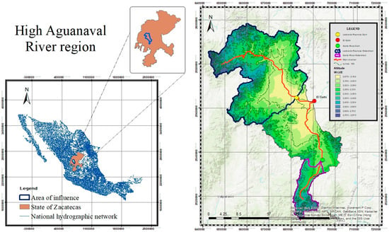
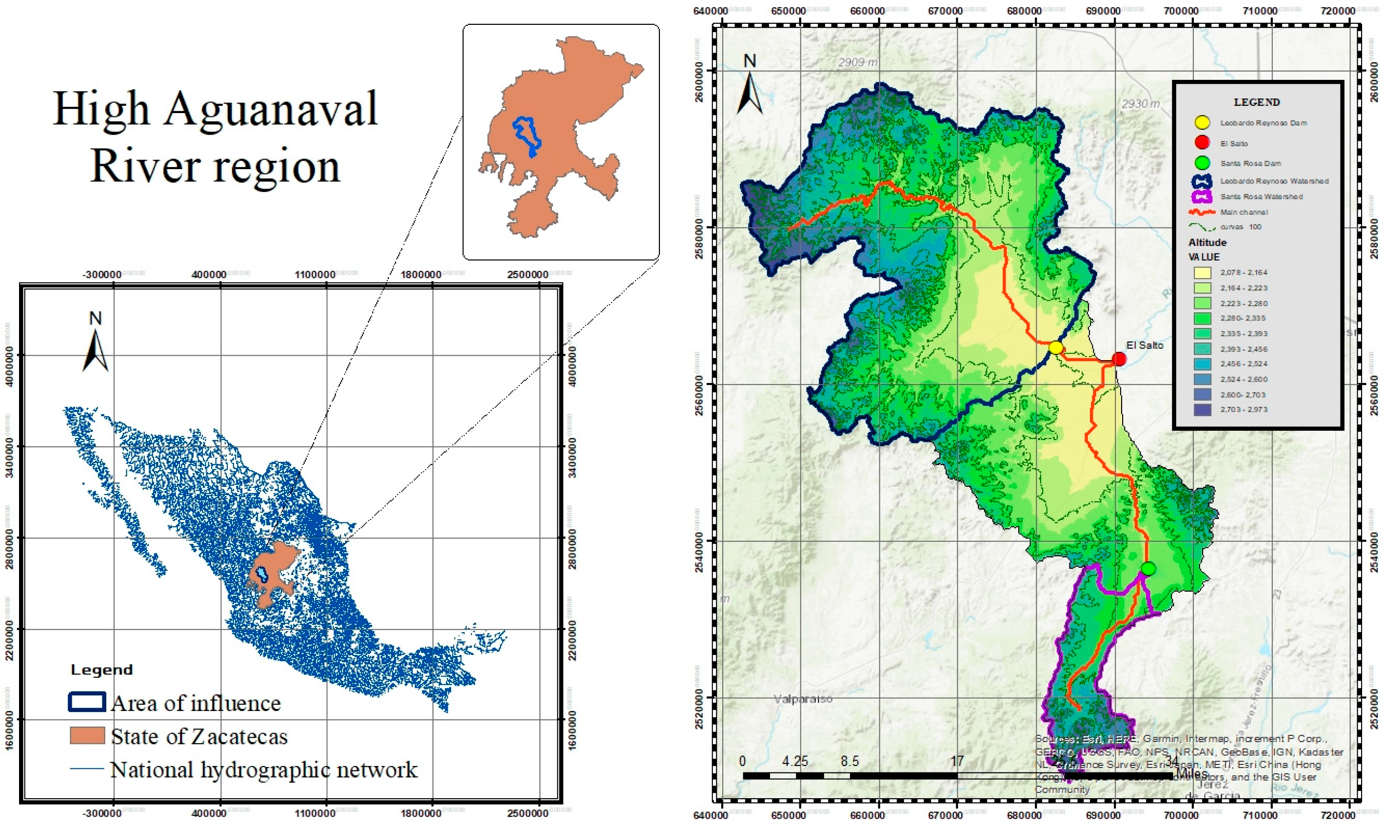
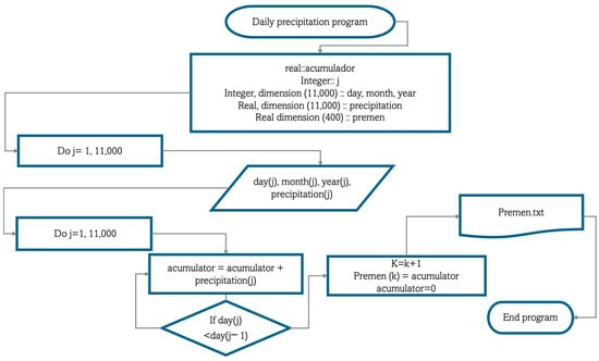
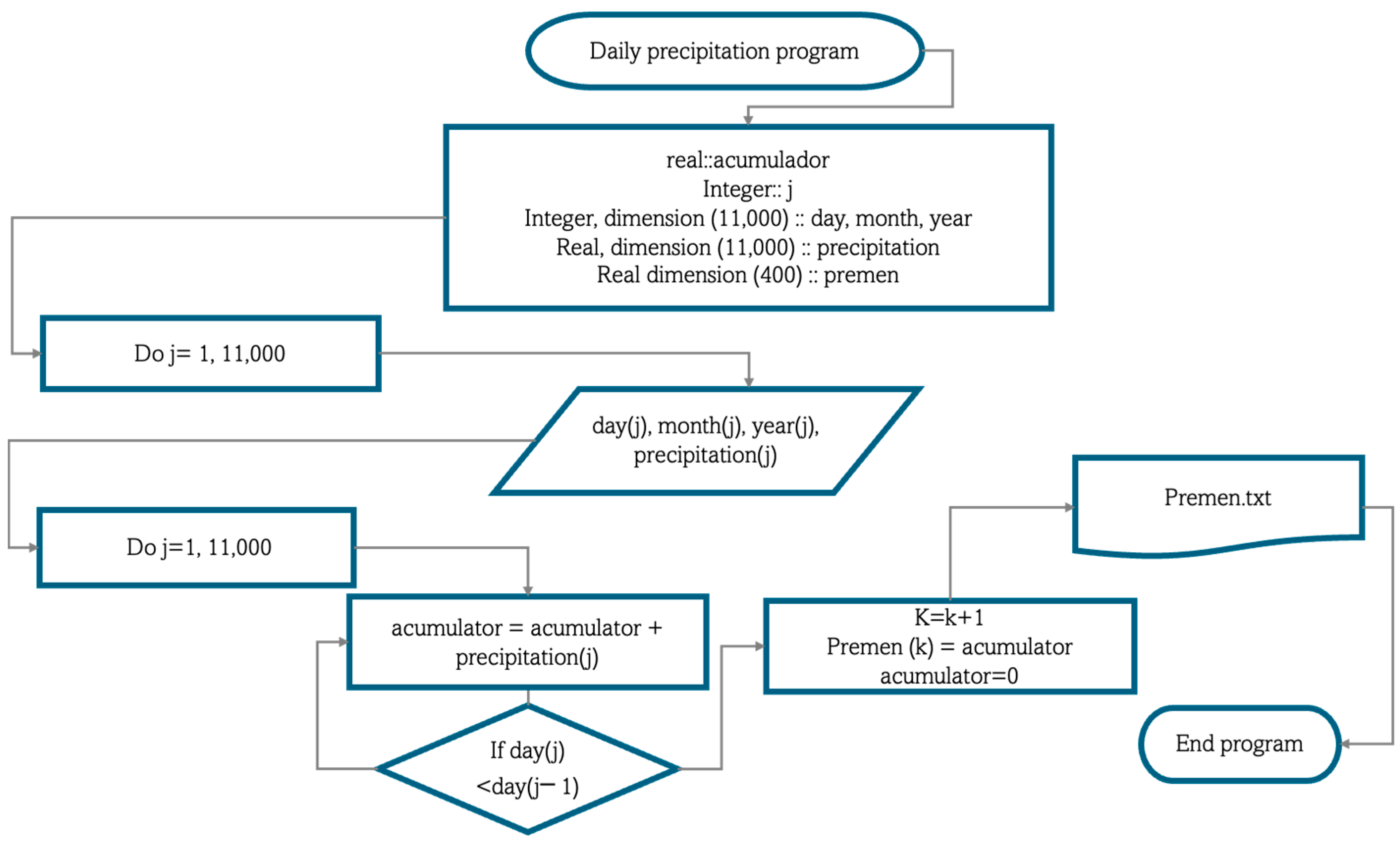
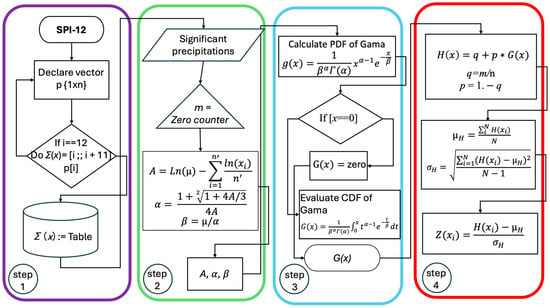
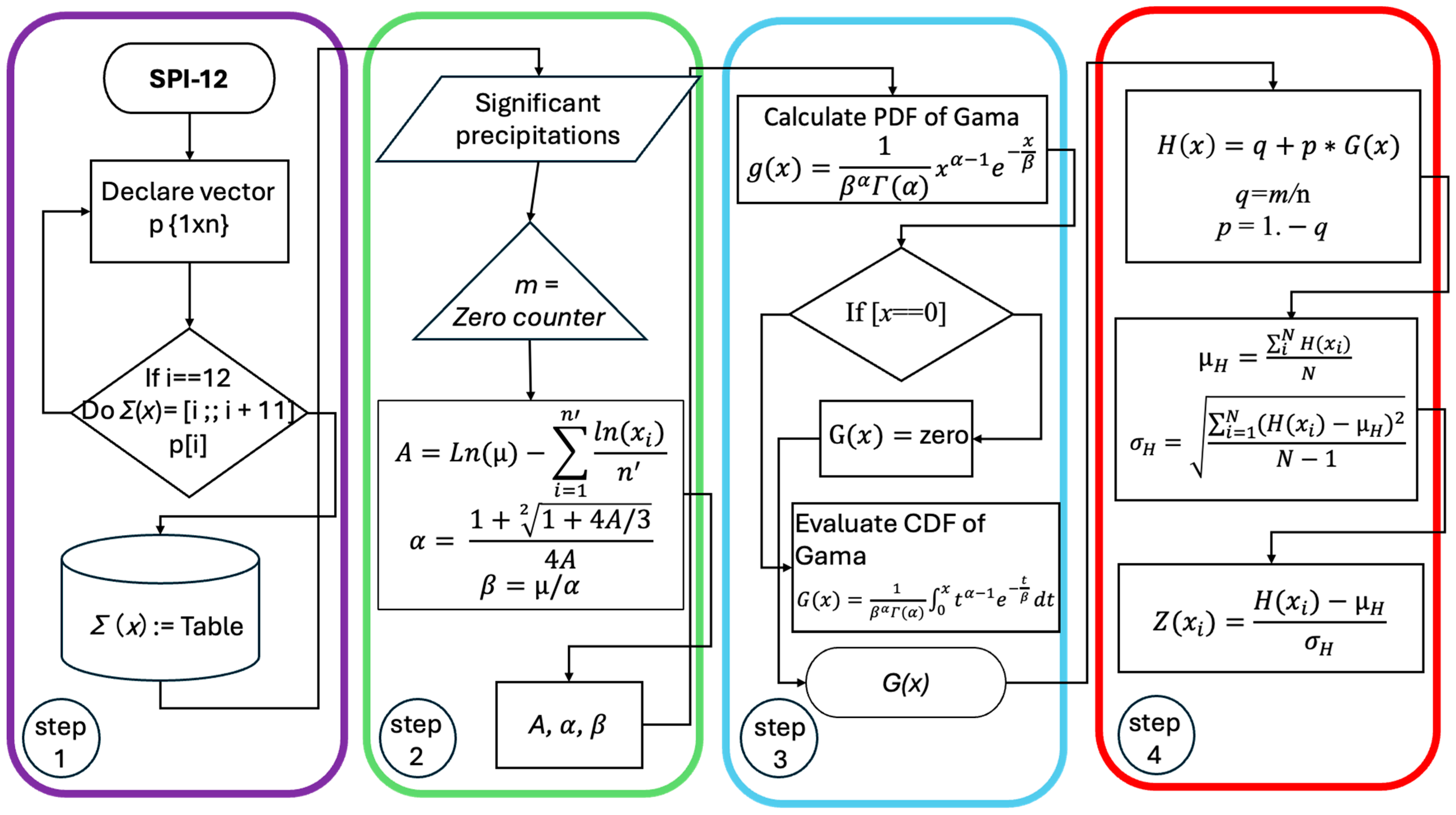
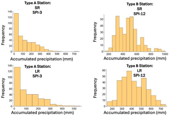
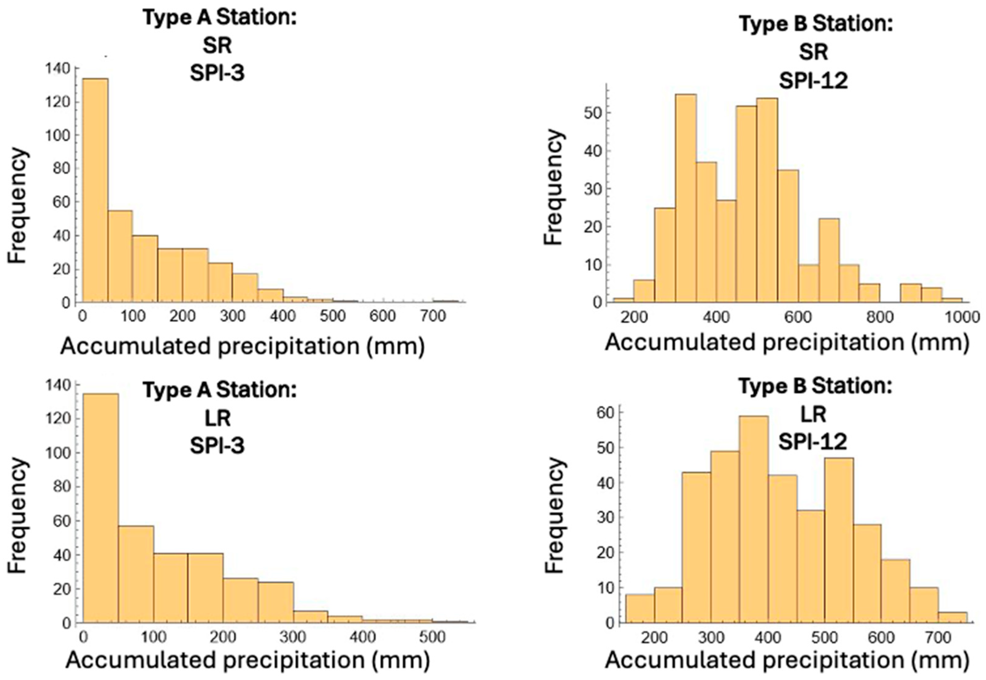
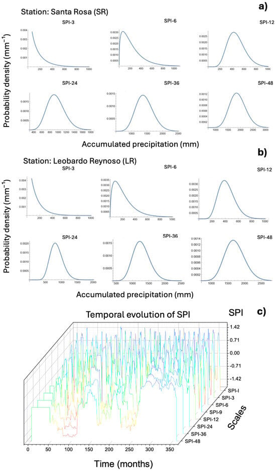
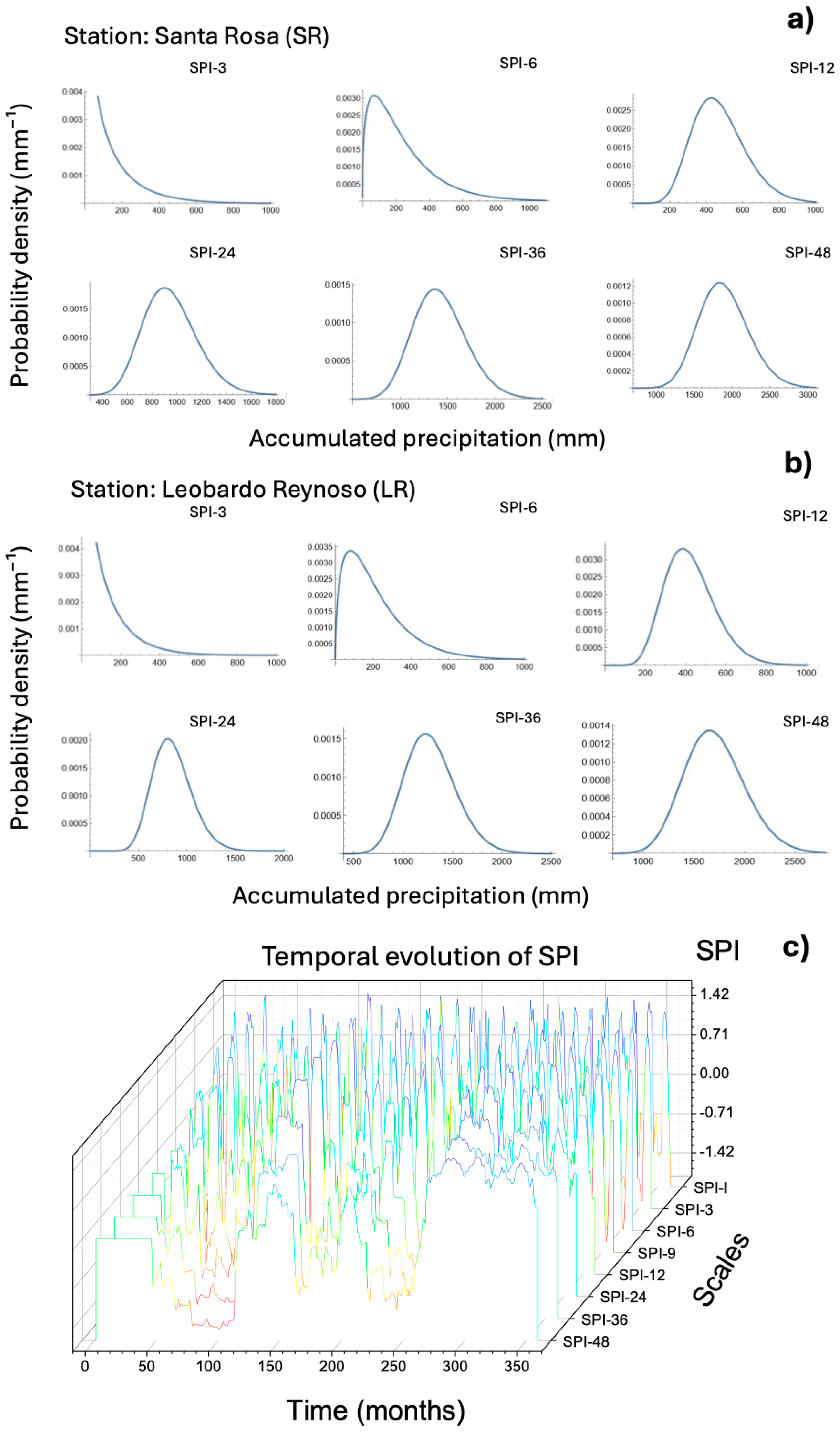
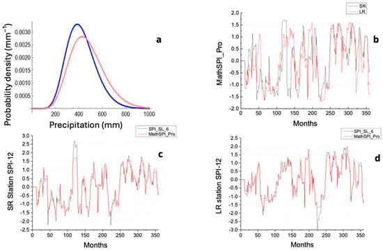
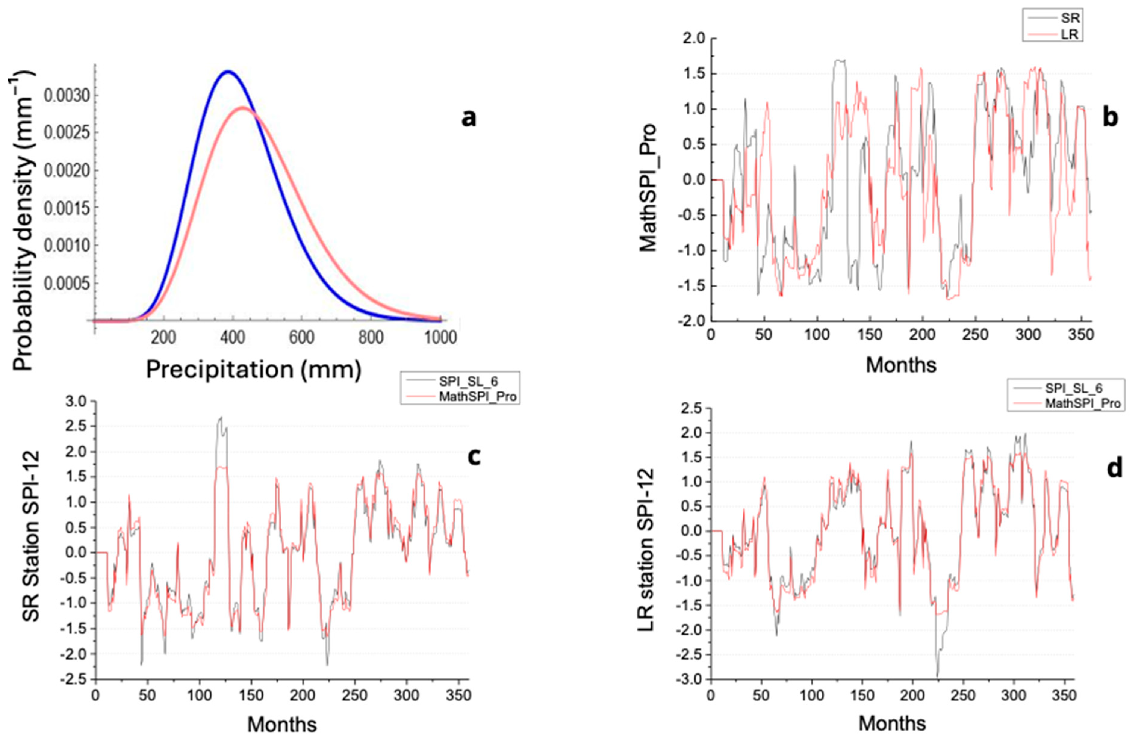
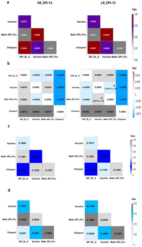
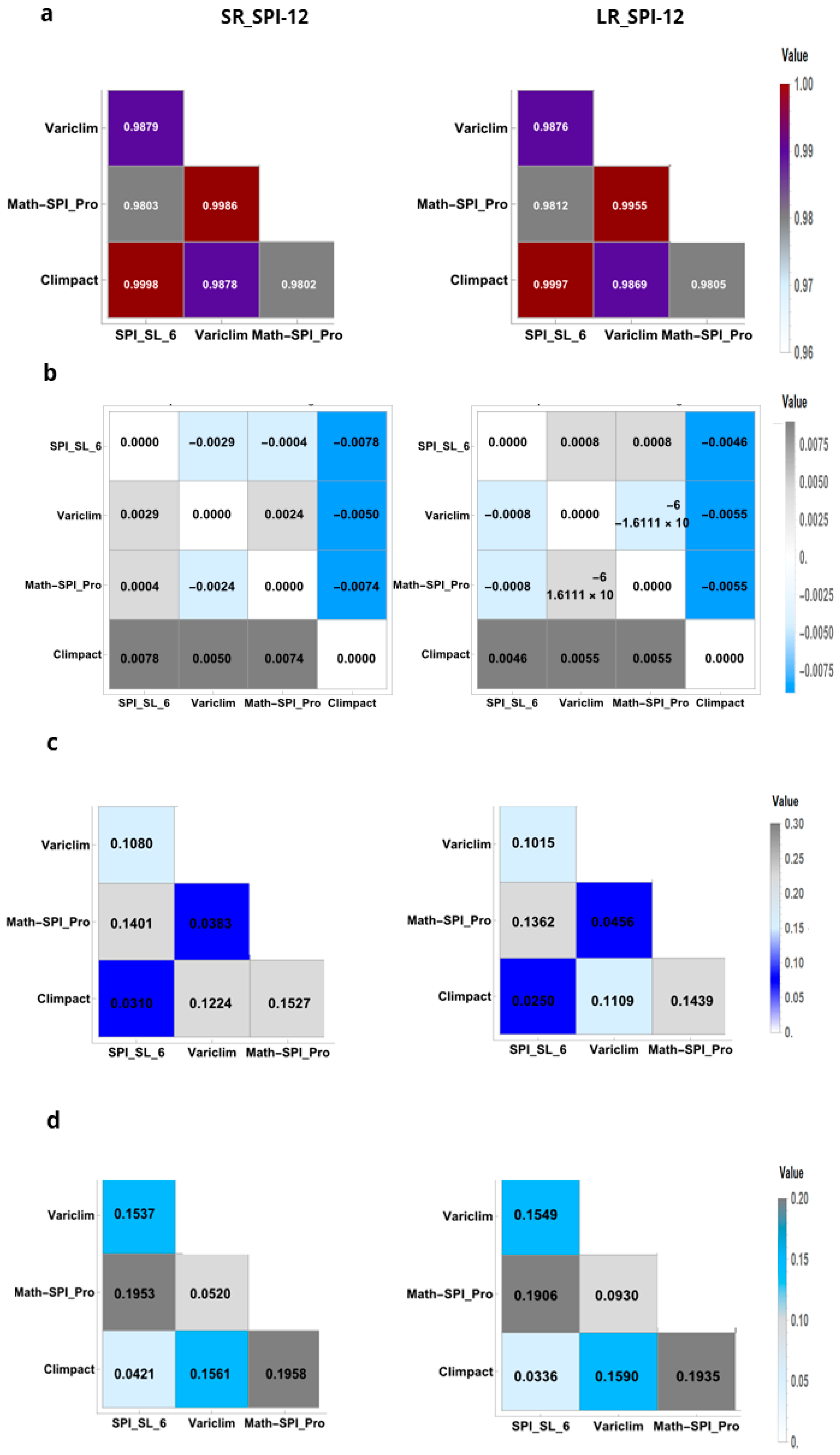
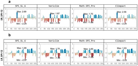
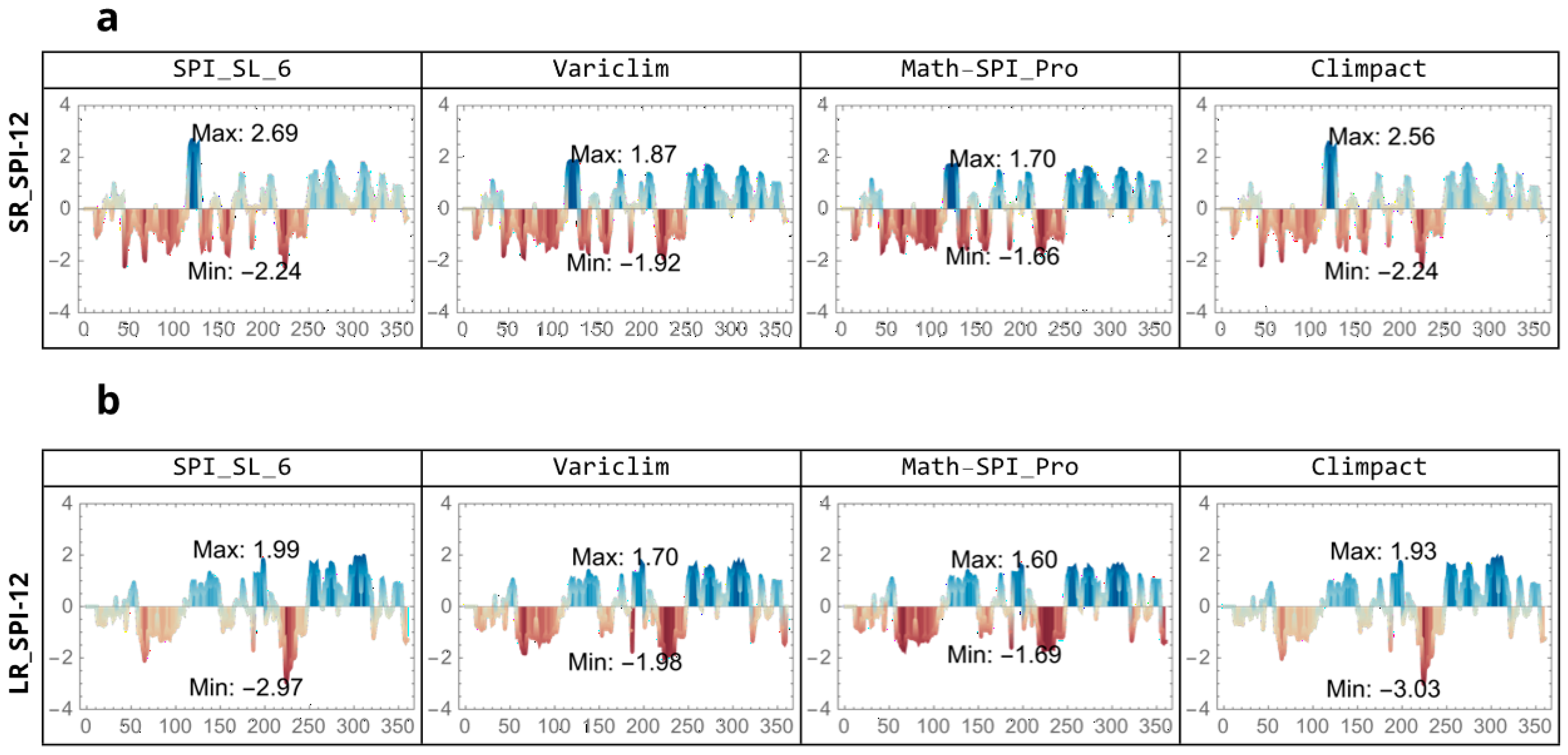
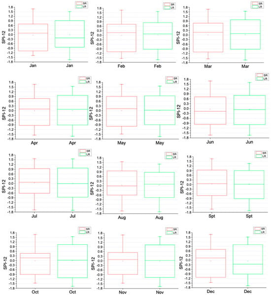
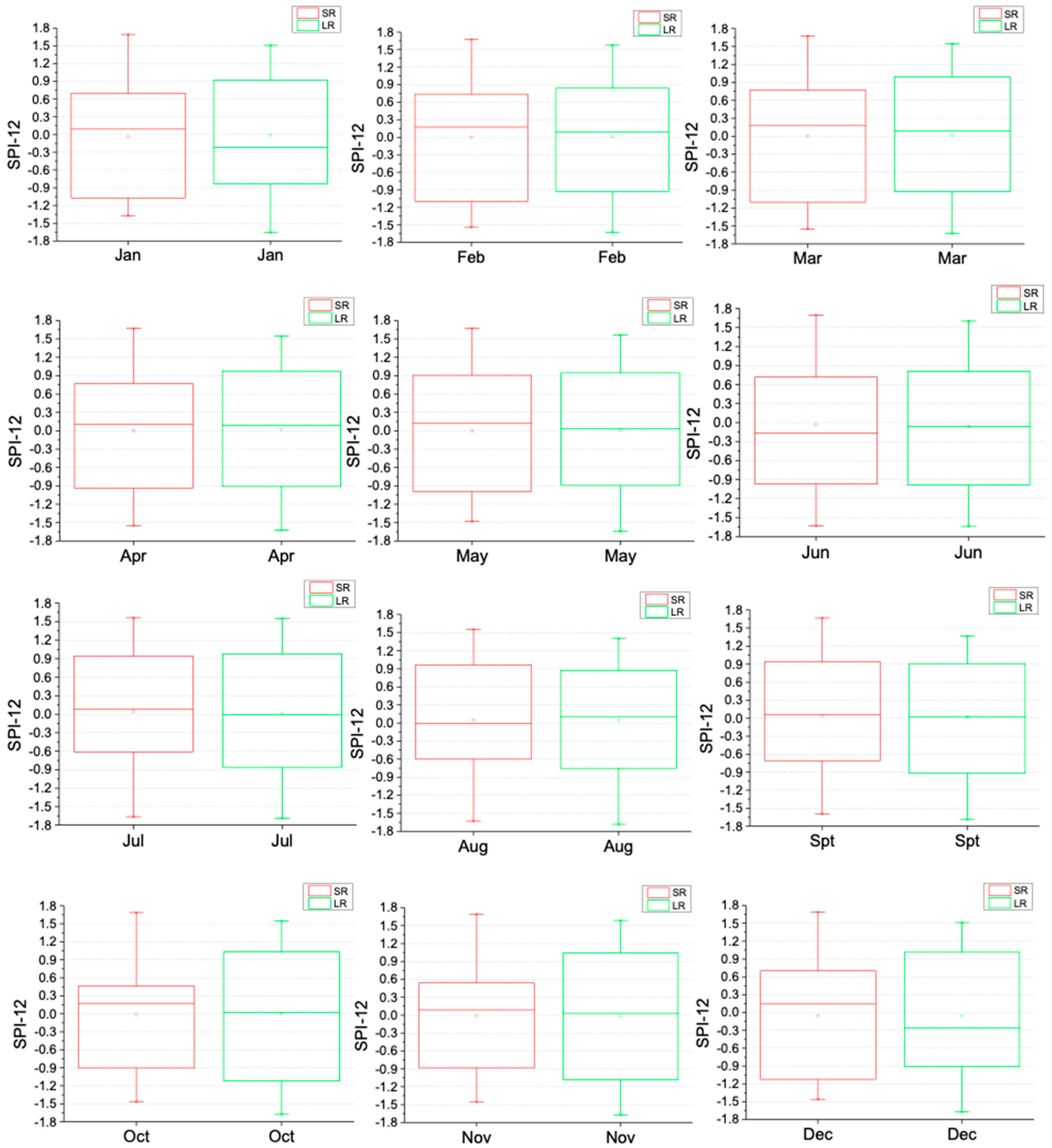

Disclaimer/Publisher’s Note: The statements, opinions and data contained in all publications are solely those of the individual author(s) and contributor(s) and not of MDPI and/or the editor(s). MDPI and/or the editor(s) disclaim responsibility for any injury to people or property resulting from any ideas, methods, instructions or products referred to in the content. |
© 2026 by the authors. Licensee MDPI, Basel, Switzerland. This article is an open access article distributed under the terms and conditions of the Creative Commons Attribution (CC BY) license.