


Abstract
Urban-greening decisions require interpretable thermal evidence. We analyzed 18 clear-sky summer daytime Landsat 8/9 acquisition groups over Harbin (2022–2025), defining exterior land-surface temperature (LST) contrast as 300–500 m minus 0–200 m around mapped green features. The support-restricted reference retained 73 of 1114 candidates, with an imprecise log-area association (−0.028 °C per original SD; 95% CI, −0.583 to 0.528). An exterior-outcome-aligned analysis retained 271 features; its pooled slope was 0.166 °C (−0.017 to 0.349), whereas direct interaction-model slopes were −0.082 and 0.123 °C without resolved subset heterogeneity. Eligibility changed the analyzed population; a change in the within-subset area association was not established. Built-dominant pseudo-features had a negative median contrast (−0.962 °C), constituting a hot object rather than a neutral design-only benchmark. An exploratory built-fraction-balanced comparison gave a smaller, support-sensitive separation without identifying vegetation-specific cooling. A 224-point mapped-positive audit found 212 Green, two Non-green and ten Uncertain labels; only 13 points belonged to the reference population. Spatial holdout performance was weak (R2 = −0.060). These results support explicit eligibility and background reporting, not causal cooling estimates, optimal park sizes, validated cooling distances or transferable design thresholds.
1. Introduction
Urban vegetation can modify surface energy exchange through shading, evapotranspiration, albedo and aerodynamic processes [1,2,3,4]. Global studies have documented spatially unequal surface cooling associated with green spaces [5], while syntheses show that climate, urban morphology and tree traits condition cooling performance [6]. Air-temperature research also demonstrates the relevance of trees to urban heat [7]. These findings motivate greening, but they do not imply that a satellite surface-temperature difference is a direct measure of air-temperature change or human heat exposure [8,9,10].
The comparison background is part of the measured outcome, rather than a neutral analytical backdrop. Climate and impervious surfaces influence urban thermal patterns [11,12,13], and recent research explicitly distinguishes internal park characteristics from external drivers of measured park cooling [14]. Methodological and sensing reviews document heterogeneous cooling definitions, comparison zones and observational scales [2,3,15,16]. Previous studies have generally examined feature size, cooling metrics, comparison zones or spatial scale as separate analytical choices. The present contribution is different: it treats eligibility, ownership, background composition, crossed dependence and geographic prediction as a connected measurement-design problem and tests how that chain limits sustainability inference.
Area-related cooling and design thresholds remain active topics. Studies of park size, landscape configuration and cooling extent [17,18,19] have been extended to multi-city benefit–cost relationships and nonlinear two- and three-dimensional predictors [20,21]. Cooling associations also vary across latitude, meteorological settings and cities [22,23,24,25]. Harbin is already represented through satellite, field and landscape-metric studies [26,27,28]. For sustainable planning, however, a threshold or design rule is useful only if its eligible population, spatial support and transfer domain are explicit. Against this regional evidence, we test whether a conservative thermal-support workflow represents the mapped candidate population and whether its conclusions persist under explicit changes to eligibility and comparison definitions.
This issue is particularly consequential when fine-resolution land-cover boundaries are combined with medium-resolution thermal data. Landsat surface-temperature products are distributed on a grid finer than the native thermal measurements [29,30,31]. Resampling does not supply additional independent thermal observations, and a common analysis grid does not remove point-spread-function overlap or spatial autocorrelation [8,9,32]. Requiring internal thermal support may improve confidence in within-feature temperature but unnecessarily restrict an outcome defined entirely outside the feature. Conversely, relaxing internal support cannot guarantee that exterior observations are free of mixed pixels or neighboring green-space influence.
We analyzed local exterior land-surface-temperature (LST) contrasts around mapped green features in Harbin over four summers. We asked three questions: RQ1, how strongly does thermal-support screening alter the mapped feature population? RQ2, how sensitive is the estimated area association to eligibility and background definition? RQ3, does the fitted association transfer to spatially unseen mapped features? We retained the original support-restricted analysis as a reference and evaluated an exterior-outcome-aligned analysis alongside it. Additional background-composition, ownership, influence and spatial-partition checks were post hoc sensitivity analyses. The estimand is an adjusted association for a specified exterior LST difference; it is not the causal effect of creating or enlarging a park.
2. Materials and Methods
2.1. Study Area and Operational Urban Domain
Harbin is a cold-region city in northeastern China centered near 45.72° N, 126.64° E. The municipal administrative boundary from FAO Global Administrative Unit Layers 2015 was used only as a search frame. To prevent detached towns and rural water bodies from entering the same analysis as the main city, the model domain was derived from the 2020 Global Human Settlement Layer Settlement Model [33]. Cells classified as dense urban clusters or urban centers were joined with eight-neighbor connectivity. Components containing urban-center cells were retained, and the largest component was selected without reference to any temperature outcome. The resulting core covered 467.94 km2. The primary sampling domain was the core plus a 5 km fringe clipped to the administrative frame (1161.51 km2); a 3 km fringe was retained for sensitivity analysis. A 6.5 km halo supported extraction of full feature geometries and exterior cells. All geometry, distance and area calculations used WGS 84/UTM zone 52N (EPSG:32652). The 5 km fringe is an operational urban–peri-urban sampling choice, not an estimated thermal influence distance. The 3 km and core-only analyses assess domain dependence; they do not validate 5 km as a physically optimal boundary.
2.2. Mapping Blue and Green Features Using Multiple Products
Candidate features were mapped on a 10 m grid using four distinct, potentially correlated product families: ESA WorldCover 2021 [34], JRC Global Surface Water [35], GLC_FCS30D 2022 [36] and Dynamic World observations from the summers of 2022–2025 [37]. Google Earth Engine was used for source harmonization and raster processing [38]. Blue support required at least three of four votes. The four votes were WorldCover water, GLC_FCS30D water, persistent JRC water (occurrence at least 75% and seasonality at least 10 months) and Dynamic World water probability of at least 0.5 based on at least 10 observations. Green support required at least two of three votes from WorldCover vegetation classes, GLC_FCS30D non-crop vegetation classes and a Dynamic World sum of tree, grass and shrub probabilities of at least 0.5, with crop probability below 0.2 and at least 10 observations. Green cells overlapping the primary blue mask were removed. WorldCover vegetation codes were 10, 20 and 30, and its water code was 80. GLC_FCS30D vegetation codes were 51, 52, 61, 62, 71, 72, 81, 82, 91, 92, 120, 121, 122 and 130; water was 210 and built land was 190. The 2022 GLC_FCS30D band was used. Dynamic World probabilities were calculated as the median of four annual June–August mean probability images, with at least 10 contributing observations pooled across the four summers. Categorical products were harmonized by nearest-neighbor sampling to the 10 m working grid; this did not upgrade the resolution of the 30 m inputs. Multi-product agreement is not independent reference validation [39]. These temporally heterogeneous products define a fixed consensus mask, not independently verified persistent boundaries for every thermal acquisition.
The resulting units are termed mapped green features, not verified parks, managed urban green spaces or natural ecological patches. Eight-connected components of at least 0.5 ha were vectorized. Membership in the primary domain was determined by each feature’s representative point, while area and shape were computed from its unclipped geometry. The shape index was defined as perimeter divided by twice the square root of pi times area; a circle therefore has a value of one and more complex shapes have larger values. OpenStreetMap polygons and water lines supplied auxiliary semantic labels but did not modify candidate geometry because coverage was incomplete. Geometry was treated as static for all 18 acquisitions, although WorldCover 2021, GLC_FCS30D 2022 and Dynamic World 2022–2025 do not establish boundary persistence on every date. Classification or boundary error can therefore alter area and shape, determine whether internal support is met, change cell ownership and shift distance-zone membership; it is not confined to a single predictor. The consensus rules yielded 1559 features in the support halo and 1309 in the primary domain before thermal-support screening, comprising 1114 green and 195 blue features (Figure 1).
Figure 1.
Study location, operational urban domain, and mapped feature populations in Harbin. (a) Location of Harbin within Heilongjiang Province, northeastern China. (b) The GHSL 2020 contiguous urban core, the core + 3 km sensitivity domain, and the core + 5 km primary domain. A Sentinel-2 Surface Reflectance true-color image acquired on 1 July 2024 is shown solely as cartographic background and was not used in the thermal analysis. (c) Spatial distribution of the mapped green-feature populations and mapped blue context within the primary domain, including support-restricted reference features, exterior-outcome-aligned-only features, and other green candidates. Domain membership was assigned using feature representative points, whereas complete feature geometries are displayed. The displayed mapped-feature boundaries are analytical inputs rather than independently validated reference boundaries. All metric analyses were conducted in EPSG:32652.
2.3. Landsat Acquisition Selection and Surface Temperature
We audited all Landsat 8 and 9 Collection 2 Level-2 scenes intersecting the support halo during June–August 2022–2025 [30]. Scenes were grouped by acquisition date and sensor, and same-date adjacent paths were mosaicked. Acquisition groups were retained when at least 80% of the support halo had jointly valid surface reflectance and surface temperature; selection did not use temperature magnitude or any feature-level contrast. Eighteen acquisition groups passed, spanning all four summers and all three summer months. Three date pairs were separated by one day (10–11 July 2024, 21–22 July 2025 and 14–15 August 2025), so 18 acquisitions do not represent 18 equally separated temporal replicates.
Surface temperature was obtained from the Collection 2 Level-2 product using the official scale factor, ST = DN × 0.00341802 + 149.0 K, and converted to degrees Celsius [30,31]. Surface reflectance used DN × 0.0000275 − 0.2. Pixels were excluded when any QA_PIXEL bit from 0 to 5 was set, when QA_RADSAT was nonzero, or when required optical or thermal bands were missing. Continuous measurements and validity fractions were then aggregated to a fixed 100 m grid. A cell entered a date-specific analysis only when valid surface-temperature coverage was at least 80%, surface-temperature uncertainty (ST_QA) was no greater than 5 K and cloud distance (ST_CDIST) was at least 1 km. The 5 K cutoff was a permissive pre-outcome exclusion rule, not a claim that uncertainty was small relative to the observed contrast. We therefore reconstructed the reference outcome at ST_QA cutoffs of 4, 3 and 2.5 K. These rules and sensitivities were applied without selecting a threshold from the resulting coefficient.
2.4. Thermal Support, Cell Ownership and Outcome Definition
A geometric support audit placed an axis-aligned 100 m square proxy over each feature under nine phase offsets. The support-restricted reference analysis required at least one footprint with at least 80% feature coverage in six of nine phases and at least one actual internal cell on the fixed grid. This rule was retained as the primary reference because it was the frozen original specification and guards against interpreting geometrically unresolved features as well-measured spatial units. It is not intrinsically aligned with an entirely exterior response; it favors larger features, and it is not a reconstruction of the sensor point-spread function. The exterior-outcome-aligned analysis was therefore required to assess this source of selection rather than to replace the reference post hoc. Frozen denotes the retained original workflow, not prospective registration. The direction or precision of the exterior point estimate was not used to replace the primary population after results were known.
At 10 m resolution, each supported exterior pixel was linked to its nearest mapped blue or green source by a Euclidean distance transform. Sources smaller than the 0.5 ha feature threshold still acted as competing sources. Within each 100 m cell, the most frequent positive candidate-owner index was selected; owner purity was its pixel count divided by all supported exterior pixels. Ties were resolved by the smallest candidate index. A cell could therefore have only one retained owner. Eligible cells had at least 80% domain support, no more than 10% mapped blue or green source fraction, and at least 50% owner purity. This rule prevented silent cell reuse, but it also made the outcome conditional on the mapped configuration and proximity of neighboring sources. It neither removed thermal interference nor made the focal feature the sole physical source of the contrast. The coverage and source-fraction thresholds limit off-domain and mapped-source contributions, while the purity threshold requires at least half of the supported exterior pixels to share an owner. These are reproducible screening conventions, not calibrated bounds on thermal mixing or guarantees of independence.
For feature p on date t, the primary outcome was
Local exterior LST contrast(p,t) = mean LST at 300–500 m—mean LST at 0–200 m.
Operational ring distance was the median nearest-source distance among the 10 m exterior pixels assigned to the selected owner inside the 100 m cell. It was not the geometric distance from the cell center to the vector boundary. Intervals were lower-inclusive and upper-exclusive: [0, 200) and [300, 500) m; cells beyond 1500 m were excluded. The near zone was chosen to characterize immediately adjacent exterior surfaces while retaining at least three 100 m cells; the 100 m gap reduced direct overlap between the two summaries. These were feasibility-driven analytical constructs, not independently validated thermal-influence distances. Both zones required at least three date-valid cells. Positive values indicate that the specified near exterior was cooler than the specified outer zone; negative values were retained. The 300–500 m zone was not assumed to be a plateau or a counterfactual without the feature. We therefore use “local exterior LST contrast,” not “cooling intensity.” The separate distance-support gate only required five rings spanning at least 400 m. It did not identify a plateau, and no cooling distance was estimated or validated. The gap does not eliminate point-spread-function overlap, spatial autocorrelation or contributions from neighboring surfaces. Alternative and offset zones assess dependence on these definitions rather than identify a unique physical cooling footprint.
2.5. Covariates and Analysis Sample
Feature area and shape index were static geometric covariates. The primary built-context covariate was the fraction of GLC_FCS30D class 190 impervious surface within 500 m of the feature boundary, aggregated to the same 100 m grid. Fractions at 300 and 1000 m and corresponding WorldCover 2021 and GHSL 2020 measures were workflow-defined sensitivities. The mean normalized difference vegetation index in the 300–500 m comparison zone was initially included as a candidate covariate. The area in hectares was natural-log transformed. Continuous predictors were centered and divided by population standard deviations over the feature-date analysis rows, so features with more valid dates contributed more to scaling. The original log-area standard deviation was 0.942994. All sensitivity-analysis coefficient comparisons used this same scaling, whereas each cross-validation fit used training-only scaling. A one-standard-deviation log-area increase corresponds to an area multiplication by exp(0.942994), approximately 2.57; an area doubling is 0.735 standard deviations.
The blue–green comparison was conditional on independent-feature count, common support and parent-feature hierarchy. Standardized mean differences greater than approximately 0.5 were treated as material imbalance. Repeated acquisition dates were not counted as additional independent features. These rules restricted inferential modeling to green features.
2.6. Statistical Analysis
The primary inferential target was the adjusted association between standardized log area and local exterior LST contrast among the 73 support-restricted reference features, estimated by the Gaussian linear mixed-effects model. Local exterior LST contrast was the response; standardized log area, shape index and 500 m built fraction plus sensor were fixed effects; and feature and acquisition date had crossed random intercepts. The model was fitted by restricted maximum likelihood for coefficients and variance components. The exterior-outcome-aligned mixed model estimated a different eligible population. GEE assessed feature-clustered covariance sensitivity, the crossed bootstrap assessed dependence on feature and date resampling in a distinct date-fixed-effect estimator, and spatial cross-validation evaluated prediction rather than coefficient validity. Maximum likelihood was used for comparisons among linear, quadratic and cubic-spline area specifications. A nonlinear model was allowed to replace the linear model only if it improved the corrected Akaike information criterion (AICc) by at least four and passed predictive and stability checks. A segmented model required stronger workflow-defined evidence and at least 30 independent features on each candidate side; it was not fitted when this gate failed. The four-point criterion was a conservative workflow choice, not a universal threshold for nonlinearity. We also report AICc differences, Akaike weights within the three-model candidate set, the quadratic term and fitted curves [40,41]. The AICc correction used feature-date observations as n; dependence makes that small-sample correction approximate. No equivalence bounds were defined independently of these outcomes, and no equivalence conclusion is drawn [42,43,44].
The initially recorded full formula included surrounding NDVI. At the independent-feature level, surrounding NDVI and built fraction exceeded the workflow-defined absolute-correlation threshold of 0.70 and shared the response’s outer-zone measurement support. The reduced formula, excluding surrounding NDVI, therefore defined the reference specification, while the full formula was retained only to quantify model dependence.
Because the reference mixed-model residuals were heavy-tailed and heteroscedastic, we fitted a feature-clustered Gaussian generalized estimating equation with date fixed effects and bias-reduced sandwich covariance [45]. We additionally fitted an exploratory Student-t residual model with crossed feature/date random intercepts; its Gaussian counterpart checked compatibility with the original mixed-model coefficient. These sensitivity models assess model dependence, not causal identification. Marginal and conditional mixed-model R2 followed Nakagawa and Schielzeth [46]. Predictive transfer to new features was assessed with spatial and random feature-level folds, keeping every date of a feature in one fold [47]. Residual Moran’s I and false-discovery-rate adjustment were used as diagnostics [48]. Software versions, seeds, numerical warnings and post hoc analysis status are detailed in the Supplementary Materials. The 911 reference and 3215 exterior observations represent 73 and 271 feature clusters, respectively; repeated rows are not independent features.
2.7. Sensitivity Analyses of Selection and Comparison Backgrounds
We compared all primary-domain green candidates, and internally supported candidates and analyzed features using medians, interquartile ranges, 5th–95th percentiles and standardized mean differences. Each difference compared retained with excluded candidates, dividing the mean difference by the square root of the average of the two sample variances. Feature-level distributions, rather than repeated rows, were used for selection summaries. Core and fringe membership used the representative point and the same outcome-independent domain boundaries.
For the exterior-outcome-aligned analysis, we removed both the geometric internal-footprint proxy and the actual internal-cell requirement while retaining domain membership, complete geometry, exterior ownership and purity, date-specific quality thresholds and at least three valid cells per outcome zone. The 73 reference features were nested within the 271 exterior features. A direct model fitted standardized log area, a reference-subset indicator and their interaction, with the same adjustment covariates and crossed feature/date intercepts. We report the subset main effect at standardized log area zero and both slopes derived from this single model, using its covariance matrix for the reference-slope interval. This post hoc interaction tests conditional slope heterogeneity; subset membership is not randomized, and area distributions overlap only narrowly near the reference scaling point. Other proxy-only and quality sensitivities are specified in the Supplementary Materials. Writing the relevant fixed terms as b_A z + b_S S + b_AS zS, where S = 1 denotes the reference subset and z is original-standardized log area, the non-reference slope is b_A, the reference slope is b_A + b_AS, and the subset difference at z = 0 is b_S. The main effect is therefore a conditional level contrast, not an average population difference or an intervention effect.
Three alternative outcomes compared [0, 100) with [300, 500), [0, 200) with [500, 700), and [100, 300) with [500, 700) m under the original support rule. In addition, to reduce immediate boundary adjacency in the expanded exterior population, we fitted the [100, 300)/[500, 700) m outcome to every exterior-eligible feature. These analyses probe spatial support and potential point-spread-function leakage; they do not remove the sensor point-spread function or provide matched independent non-green controls.
We compared reference features with two outcome-blind translated-polygon benchmarks. The originally submitted built-dominant pseudo-features preserved polygon area and shape, urban zone and 500 m annular built context (absolute caliper 0.10), but required internal built fraction ≥0.50 and no mapped blue/green source overlap. Thus, they represent a built hot-object comparison, not a thermally neutral or design-only placebo. An additional exploratory placement matched the same geometry, zone and annular context while constraining static 2022 built fractions between the pseudo-interior and 0–200 m ring, and between the 0–200 and 300–500 m rings (each absolute difference ≤0.10); a further sensitivity retained only pseudo-features balanced on the ultimately owned ring cells. Placement never read LST. Both constructions reran nearest-source ownership and the frozen date-specific quality rules. Observed and pseudo contrasts were paired by feature and acquisition date, with 1999 crossed feature/date bootstrap replicates. The offset [100, 300)/[500, 700) m outcome was also checked. Neither benchmark balances canopy, morphology, emissivity or unmapped sources sufficiently for causal attribution; full algorithms and support counts are in Section S17. Feasibility is established by the completed balanced placement; its interpretation is limited by incomplete balance and by changes in the feature–date support, not by a claim that the pseudo-sites are thermally neutral.
Exact Landsat acquisition times were retrieved from Collection 2 Level-2 STAC records; the mean time was used for two-scene mosaics. ERA5 hourly air temperature, relative humidity, dew point, precipitation, 10 m wind speed and shortwave radiation were obtained for the primary-domain centroid (requested 45.710° N, 126.639° E; returned grid point 45.75° N, 126.75° E) [49]. Nearest-hour values and preceding 24, 48 and 72 h precipitation totals were recorded. After inspection of the original results, five exploratory one-weather-at-a-time mixed models added standardized acquisition-time air temperature, humidity, wind, shortwave radiation or 24 h precipitation, each with its main effect and area interaction. These models retained crossed feature/date intercepts; weather varies over only 18 dates and the Wald intervals were not multiplicity-adjusted.
We audited a pre-drawn stratified sample of 224 of 1114 mapped-positive green candidates across 18 area × urban-zone × built-context strata, retaining inclusion probabilities and design weights. Two coauthors interpreted Google Earth imagery dated 14 August 2025 for all points, as confirmed retrospectively by the authors. The protocol required separate initial Green, Non-green or Uncertain labels without consulting the other reader’s labels or thermal/model outcomes. Both reader sheets and the sole adjudication were retained, and labels were cross-tabulated with the analyzed feature sets. This audit addresses mapped-positive class identity, not omission or boundary accuracy. Metadata provenance and variance limitations are documented in Section S18.
Crowding was assessed using boundary-to-boundary distance to the nearest other mapped green feature and the fraction of each feature’s exterior 500 m geometric buffer occupied by other mapped green features. The latter used all mapped green features in the support halo and was computed without temperature values. We fitted an additional adjustment model and examined a greater than 500 m nearest-green separation subset. This subset contained only 14 features and was not fitted under the sensitivity workflow’s exploratory minimum of 15; that minimum is a pragmatic guardrail, not a general sample-size justification. Core-only, core-plus-3 km and built-fraction-at-least-0.10 subsets tested the operational urban-domain restriction.
2.8. Crossed Dependence and Predictive Evaluation
To complement feature-clustered GEE, we independently resampled the 73 features and 18 acquisition dates with replacement and multiplied their sampling counts to weight observed feature-date rows. We generated 1999 crossed bootstrap replicates of a date-fixed-effect ordinary least-squares regression, retaining the original predictor scaling. Weighted within-date demeaning removed date intercepts before each fit. Percentile intervals were calculated from the replicate coefficients. This pigeonhole-style resampling accounts for both clustering axes as a sensitivity [50,51] but is not a bootstrap of the mixed-model estimator and has limited date-cluster depth. It does not resolve spatial dependence between different features. Separate date regressions used HC3 intervals, while omission diagnostics refitted the mixed model after each date or year was removed.
Spatial validation used five feature-level folds from centroid coordinates standardized over features. The first center was the lexicographically smallest coordinate; subsequent centers used farthest-point selection, and Lloyd updates ran for up to 100 iterations. The saved folds were not balanced by area or built fraction, and initially no exclusion buffer separated training from testing. All observations of one feature stayed in one fold. Predictor centering and scaling were re-estimated using training rows only. Held-out feature random effects were set to zero; date effects were estimated from training features on the same acquisition dates. Therefore, the test concerns new features under observed acquisition conditions, not future dates or another city [47,52,53,54]. All fold convergence flags and warning messages were retained. Predictions from warning-bearing fits are reported as diagnostics rather than treated as validated operational performance; non-converged random-fold results are not corroborating evidence.
2.9. Paired Background Composition
We calculated near- and outer-zone composition on the same date-valid, uniquely owned cells contributing to each contrast. The built fraction was sampled from the georeferenced 100 m GLC_FCS30D 2022 built raster. NDVI, normalized difference built-up index (NDBI) and modified normalized difference water index (MNDWI) used the corresponding valid optical measurements; their valid-cell counts were retained separately. These indices are not class fractions. Mapped water and green fractions were computed by averaging the 10 m consensus masks within each 100 m cell. The other-green fraction subtracted the focal green polygon’s intersection area from the total mapped green area. This geometric subtraction does not validate the map. Crop and bare-land fractions were not available from the local class exports.
For every variable, we calculated outer-minus-near differences and reported means, medians and interquartile ranges. We presented both feature-date summaries and equal-feature summaries obtained by first averaging each feature across its observed dates. Standardized differences divided the paired mean difference by the square root of the mean of the two zone variances. Models separately added Δbuilt and ΔNDVI, then included both; a further model added Δother-green where it varied. A water-difference term was not estimable because the mapped water fraction was zero in all retained outcome cells. New predictors were standardized using the reference sample and the same scaling was applied to the exterior sample. Pearson correlations and variance-inflation factors (VIF) were evaluated at row and feature-mean levels. Specifications were not selected by p value. After adjustment, the area coefficient is the conditional association between log area and the thermal contrast among observations with the same measured zone-composition differences under the fitted model. Because these differences are constructed from the same spatial zones and share optical-validity support with LST, they are neither conventional independent confounders nor separable causal contributions.
2.10. Ownership and Mapped Water Context
To audit exterior support before the final ownership filter, we enumerated 100 m cell centers outside each candidate polygon within geometric [0, 200) and [300, 500) m annuli, retaining source-fraction and domain-support thresholds. We counted centers retained by the focal owner, assigned to a different retained owner, or unassigned. These categories sum to the candidate denominator. Unassigned cells cannot be attributed uniquely to ownership competition. Retention fractions and purity summaries used this common geometric candidate set; operational owned-cell counts continued to use the within-cell median-distance rings. The two supports were intentionally distinguished. Spearman correlations described associations with area, shape, nearest-green distance, neighboring green fraction and built context without treating the spatially correlated features as independent tests.
We also measured polygon-to-polygon distance to the union of mapped blue candidates in the support halo. We used all such water features rather than assigning an unsupported major-water threshold or assuming that every blue polygon represented the Songhua River. A log(1 + distance in meters) covariate was added separately to each eligibility model, using reference-sample scaling. This is a mapped-water context sensitivity, not independent water-geometry validation. A shared-cell response model was not fitted because the resulting cross-feature measurement covariance was not established.
2.11. Influence and Curvature Stability
Influence analysis used two explicit thresholds fixed from the full reference fit: an absolute conditional residual greater than three sample residual standard deviations and greater than three model-error standard deviations, where the latter equals the square root of the estimated residual variance. The second threshold reproduces the original diagnostic. We refitted after excluding flagged rows and, separately, all observations of flagged features. These outcome-dependent exclusions are sensitivity analyses, not corrections to the primary dataset; no iterative removal was performed.
For curvature stability we added squared standardized log area to the date-fixed-effect OLS specification and generated 1999 crossed feature/date bootstrap replicates, using the same within-date weighted demeaning as in the linear sensitivity. The percentile interval assesses curvature in this marginal specification, not in the crossed mixed model itself. All linear, quadratic and spline likelihood comparisons were retained irrespective of the bootstrap result. No breakpoint or optimum was estimated.
2.12. Spatial Holdout Sensitivity
The 73-feature reference population was evaluated under the original five spatial folds and three additional outcome-blind centroid partitions. Full partition procedures, fold membership and numerical status are documented in Section S13. These reuses of one feature set are diagnostics, not independent validation replicates.
3. Results
3.1. Thermal Screening Selected a Different Feature Population
The primary domain contained 1309 mapped features: 1114 green and 195 blue candidates. The original geometric-plus-fixed-grid internal-support rule retained 271 green features, and 73 of these yielded at least one valid exterior contrast (911 repeated observations across 18 dates). Retention was 73/1114 (6.55%) against all mapped green candidates but 73/271 (26.94%) conditional on original internal resolvability. An area-only lower bound of 0.8 ha left 839 candidates, of which 73 (8.70%) were analyzed; area alone does not establish thermal resolvability. Candidate median area was 1.47 ha (IQR, 0.80–3.42), compared with 6.83 ha (4.53–12.51) among internally supported features and 6.84 ha (4.63–13.59) in the analysis. Thus, the selection result depends on the denominator and altered the feature population, not merely precision (Table 1, Tables S2 and S3; Figure 1 and Figure 2).
Table 1.
Sample flow under support-restricted and exterior-outcome-aligned eligibility.
Figure 2.
Eligibility changes feature representation. (a) The original route has 1114 candidates, 271 internal-support candidates and 73 reference features; percentages refer to all candidates. The exterior-outcome-aligned route is separate and retains 271 features, but these are not the same 271 internal-support candidates. Counts denote mapped features, not repeated rows. (b) Area ECDFs give each feature equal weight. No distributional hypothesis test is implied.
Only 25 of the 73 analyzed features were inside the GHSL core; 33 were in the 0–3 km fringe and 15 in the 3–5 km fringe. The study therefore concerns an operational main-urban domain including a peri-urban fringe, not a sample exclusively drawn from the dense urban core. The exterior-outcome-aligned analysis retained 24.327% of green candidates and yielded 271 features and 3215 observations. All 73 reference features were contained in this exterior population. The identical count of 271 at the earlier internal-support stage is coincidental: that stage precedes exterior quality screening and does not have the same membership.
The two reader columns agreed for 223 of 224 mapped-positive samples (99.55%; Cohen’s κ = 0.956). After the sole disagreement was adjudicated, labels were 212 Green, two Non-green and ten Uncertain; design-weighted proportions were 94.67%, 0.89% and 4.45%, respectively. This full-frame mapped-positive estimate must not be applied directly to either analyzed subset. Of the 73 reference features, 13 happened to be sampled and all 13 were labeled Green. Of the 271 exterior-outcome-aligned features, 48 were sampled (45 Green, one Non-green and two Uncertain); 54 of the different, original internal-support 271 were sampled (52 Green, two Uncertain). These intersections are descriptive and too small, particularly for the 73-feature subset, to establish boundary or subset-wide classification accuracy (Table S26).
3.2. Contrasts Were Heterogeneous, and Area Estimates Remained Uncertain
The median of the 73 green-feature median contrasts was 0.604 °C (interquartile range, −0.189 to 2.074); 26 features had negative medians (Figure S7a). Blue features were retained descriptively: their median was 0.167 °C (−0.283 to 2.706), with 5 of 12 medians negative. The blue sample had inadequate independent-feature depth, partly shared water hierarchy and appreciable covariate imbalance. It was not used to estimate an adjusted blue–green difference.
The reference mixed-model log-area coefficient was −0.028 °C per original standard deviation (95% confidence interval, −0.583 to 0.528; p = 0.922), and the shape coefficient was 0.265 °C (−0.253 to 0.783; p = 0.316). On an area-doubling scale, the estimated contrast difference was −0.020 °C (−0.429 to 0.388). These intervals include associations in both directions and do not demonstrate thermal equivalence or negligible effects. Feature-clustered GEE gave similar area estimates (Table 2). Date-fixed-effect OLS with crossed feature/date bootstrap gave an area coefficient of 0.024 °C (percentile interval, −0.619 to 0.597), with all 1999 replicates estimable (Figure S7b).
Table 2.
Reference associations with the primary exterior LST contrast.
Continuous coefficients are degrees Celsius per original feature-date standard deviation. Mixed-model intervals are Wald intervals; GEE uses feature clusters, date fixed effects, exchangeable working correlation and bias-reduced sandwich covariance.
The separately fitted exterior-outcome-aligned model gave a pooled area coefficient of 0.166 °C per original SD (95% CI, −0.017 to 0.349; 271 features, 3215 repeated observations), whereas the support-restricted reference fit gave −0.028 °C. In a single 271-feature interaction model, the non-reference slope was −0.082 °C (−0.417 to 0.253), the reference-subset main effect at standardized log area zero was 0.671 °C (−0.079 to 1.421), and the area-by-subset interaction was 0.205 °C (−0.263 to 0.673; p = 0.390). The implied reference-subset slope was 0.123 °C (−0.288 to 0.534), with its interval calculated from the joint coefficient covariance. A feature-clustered GEE interaction was 0.206 °C (−0.387 to 0.800; p = 0.496). The pooled 0.166 °C slope exceeds both within-subset point estimates, consistent with a contribution from between-subset level and composition differences rather than resolved within-subset slope heterogeneity. The subset indicator is strongly associated with area, and its main effect is evaluated near the upper edge of non-reference area support; it must not be interpreted as a causal eligibility effect (Figure 3; Table S22). The 0.123 °C slope is conditional on the pooled interaction model and should not be substituted for the separately fitted 73-feature primary coefficient of −0.028 °C. Neither the interaction nor the subset main-effect interval excludes zero; the comparison supports a change in the analytical population, not a demonstrated change in the within-subset area association.
Figure 3.
Area estimates depend on eligibility and adjustment. Points show crossed mixed-model area coefficients and Wald 95% intervals under labeled specifications, all using the original log-area SD. Feature and repeated-row counts are shown separately. The two eligibility specifications are the principal comparisons; adjustment and exclusion models are exploratory sensitivities. They are not independent replications. Runtime warnings are disclosed in the Supplementary Materials; no multiplicity correction is applied. The date-FE crossed bootstrap is shown separately in Figure S7 to avoid conflating estimators.
3.3. Background Composition and Specification Changed the Estimates
The two zones differed in observed composition (Figure 4; Table 3). With equal weight per reference feature, the mean built fraction was 0.316 in the near zone and 0.429 in the outer zone, a difference of 0.114; the mean NDVI was 0.594 and 0.533, respectively, a difference of −0.061. The corresponding exterior-population differences were 0.074 and −0.042. The mapped water fraction was zero in both zones for all retained observations. The other-green fraction was sparse in near cells and zero in outer cells, consistent with the source-exclusion and ownership rules; this does not imply the absence of water or neighboring vegetation from the wider landscape.
Figure 4.
Near and outer background composition. Each point represents the time-mean composition of one reference feature (73 features); the diagonal denotes equal near and outer values. Panels show built fraction and NDVI, with observed outer-minus-near means annotated. These are descriptive paired comparisons, not independent controls or causal effects. The complete reference and exterior summaries, including mapped water and other-green fractions, are in Table S13 and the source data.
Table 3.
Equal-feature mean background composition.
These descriptive summaries first average each feature over its available dates; they do not impose an identical date set across features. Complete distribution summaries and index-specific cell counts are supplied in the Supplementary Materials and source data.
Adding Δbuilt and ΔNDVI jointly changed the reference area estimate to 0.117 (−0.172, 0.405) °C per original SD and the exterior estimate to 0.094 (−0.012, 0.200) (Figure 3; Table S14). The joint reference model associated larger Δbuilt with larger LST contrasts and larger ΔNDVI with smaller contrasts, but these are conditional coefficients on shared measurement supports. VIF reached 5.61 for the feature-mean reference design, compared with 3.00 for its row-level design (Table S15). Adding the sparse Δother-green term gave area estimates of 0.102 (−0.184, 0.387) and 0.094 (−0.012, 0.200), respectively. A Δwater coefficient could not be estimated.
In the core-only subset, the area coefficient was −0.351 °C (−1.601 to 0.898; 25 features). The core-plus-3 km subset gave −0.012 °C (−0.667 to 0.644; 58 features). Adding the other-green fraction to the original model shifted the area coefficient to −0.230 °C (−0.779 to 0.318). The built-fraction-at-least-0.10 model did not converge and is reported only as a diagnostic. The isolated subset contained 14 features, below the exploratory minimum of 15, so no regression was fitted.
Alternative near/outer definitions under the reference rule produced area coefficients of 0.010 °C (−0.638 to 0.657; 70 features) for 0–100/300–500 m and 0.133 °C (−0.608 to 0.875; 34 features) for 0–200/500–700 m. The reference 100–300/500–700 m fit did not converge. In the exterior population, however, the 100–300/500–700 m model retained 110 features and 1307 observations and gave 0.063 °C (−0.214 to 0.339; p = 0.656). This sensitivity reduces immediate boundary adjacency but does not reconstruct the Landsat point-spread function. Tightening ST_QA to 3 K retained 71 features and 637 observations and gave −0.067 °C (−0.607 to 0.474); at 2.5 K, 65 features, 332 observations and 13 dates remained, giving −0.334 °C (−0.995 to 0.327). All intervals spanned zero (Tables S5 and S23).
The built-dominant placement matched 68 of 73 reference polygons, with 58 features and 499 valid feature-date pairs. Its pseudo-interiors averaged 0.625 built fraction, and its median feature-level contrast was −0.962 °C versus 0.818 °C for the paired green features. The observed-minus-built-pseudo mean was 1.884 °C (crossed bootstrap 95% interval, 1.278–2.496), but the negative pseudo contrast identifies this as a hot-object benchmark rather than a neutral design-only difference. The exploratory built-fraction-balanced construction placed 70 polygons and yielded 63 features and 590 pairs; its pseudo median contrast was −0.032 °C and observed-minus-pseudo mean 1.044 °C (0.416–1.676). On the exact 52-feature, 357-pair common support, the built-hot and balanced gaps were 1.488 and 1.088 °C; their 0.400 °C difference had an interval spanning zero (−0.206 to 1.003). Requiring balance on source-owned ring cells left 39 features and 381 pairs, with a gap of 0.885 °C (0.189–1.645). Separately, the offset outcome applied to the full geometrically balanced construction retained 24 features and 239 pairs and gave 0.062 °C (−0.844 to 0.937). Changing support and unverified pseudo-site land cover preclude interpreting these gaps as vegetation-specific cooling (Table S24; Section S17).
The five exploratory one-weather-at-a-time models included both a weather main effect and its area interaction (Table S25). Main effects per date-level SD were −0.000 °C (95% CI, −0.169 to 0.168) for acquisition-time air temperature, −0.096 °C (−0.255 to 0.064) for relative humidity, −0.205 °C (−0.342 to −0.069) for 10 m wind speed, 0.134 °C (0.006 to 0.261) for shortwave radiation and −0.045 °C (−0.213 to 0.123) for antecedent precipitation. Area-by-weather interactions ranged from −0.049 to 0.048 °C per log-area SD per weather SD, with every Wald interval crossing zero. Because weather varies over only 18 dates, the nominal main-effect intervals and p values are exploratory, unadjusted for five models and sensitive to the crossed-effect specification; they do not establish meteorological mechanisms or invariance. Each weather main effect is evaluated at standardized log area zero and describes a conditional association at the date level; the repeated feature-date rows do not create additional independent weather realizations.
The reduced model’s built-context coefficient was positive, but the built fraction and surrounding NDVI were strongly negatively correlated at the feature level (Pearson r = −0.755). Including surrounding NDVI changed the built coefficient to −0.152 °C (−0.488 to 0.183) in the mixed model and −0.226 °C (−0.637 to 0.186) in GEE. This is a covariate-adjusted comparison on the same outcome, not direct evidence that changing the comparison-zone geometry caused the sign reversal.
3.4. Crowding Was Associated with Loss of Exterior Support
Across the 1114 mapped green candidates, median near-zone geometric retention increased from 0.333 in the small-area tertile to 0.350 in the middle tertile and 0.424 in the large tertile. Median outer-zone retention was zero in all three groups (Table S16; Figure S8). Outer retention was more closely associated with neighboring green fraction (Spearman r = −0.461) and nearest-green distance (r = 0.291) than with log area (r = 0.062). These are descriptive spatial associations, not independent significance tests. They identify accessible exterior support as an additional selection mechanism even after internal support is removed.
Adjustment for log distance to mapped water gave area coefficients of −0.024 (−0.585, 0.538) in the reference population and 0.151 (−0.033, 0.335) in the exterior population (Table S17). This adjustment did not establish a distinct Songhua River effect.
3.5. Exploratory Curvature Evidence Was Weak and Model Dependent
The quadratic model had the smallest AICc (2920.97), followed by the linear model (2922.98) and cubic spline (2924.81). Their Akaike weights were 0.661, 0.242 and 0.097, respectively, conditional on this candidate set (Table S7). The quadratic term was 0.265 °C per squared standardized log-area unit (nominal 95% interval, 0.010 to 0.519). This is evidence of possible curvature within the fitted model, not evidence against all nonlinearity. Figure 5a shows both fitted relationships and model-based uncertainty over the observed area range.
Figure 5.
Exploratory curvature and reference spatial holdout. (a) Linear and quadratic maximum-likelihood mixed-model fixed-effect curves across observed areas, with pointwise Wald 95% intervals. Shape and built fraction are fixed at their original means, sensor at Landsat 8, and random effects at zero. Bands exclude model-selection uncertainty and are not prediction intervals. No optimal area is marked. (b) The original five-fold holdout contains 911 repeated observations from 73 feature clusters. Held-out feature effects are zero; date effects use training features on observed dates. R2 equals one minus prediction squared error divided by total observed squared deviation. The diagonal is agreement. A Hessian warning qualifies this diagnostic; additional partition and buffer results are in Figure S9.
The 2.01-point improvement over the linear model did not pass the original workflow’s four-point escalation rule. That operational decision explains why segmented fitting was not undertaken; it is not a biological test of whether a threshold exists. A breakpoint location, its uncertainty and its cross-sample stability remain unestimated.
In the additional date-fixed-effect regression, the quadratic coefficient was 0.198, with a crossed feature/date bootstrap interval of −0.187 to 0.391; all 1999 replicates had full slope rank (Table S18). The nominal mixed-model quadratic interval and the bootstrap sensitivity did not supply uniform evidence for curvature across estimators. Uncertainty at large feature areas and uncertainty from model selection remain relevant; no stable threshold follows from these results.
3.6. Dependence and Influence Limited Spatial Prediction
The reference model’s feature, date and residual variance components were 2.747, 0.100 and 1.054 °C2, respectively. Conditional on the fixed effects, the feature and date intraclass-correlation fractions were approximately 0.704 and 0.026 [55]. Marginal and conditional R2 were 0.121 and 0.762. The conditional in-sample RMSE was 0.978 °C, whereas spatial holdout RMSE was 2.122 °C, MAE was 1.631 °C and pooled R2 was −0.060 (Figure 5b). All spatial fits returned convergence flags, but one fold had a non-positive-definite Hessian warning. Random feature-fold prediction gave R2 = 0.058 with two nonconverged fits and is not treated as a validated benchmark.
Residuals were heavy-tailed (excess kurtosis, 14.89) and heteroscedastic (Breusch–Pagan p = 0.0186), with 11 observations from eight features exceeding three model-error standard deviations. Date-specific HC3 area estimates ranged from −0.229 to 0.355 °C, all with intervals spanning zero (Figure S6). In additional crossed random-intercept Student-t residual models, area coefficients were −0.011 °C per original SD (approximate 95% Wald interval, −0.605 to 0.583) for the 73-feature reference and 0.186 °C (−0.003 to 0.375) for the 271-feature exterior population. The corresponding Gaussian fits recovered −0.028 and 0.166 °C. Estimated t degrees of freedom reached the imposed lower bound of three, so this is a model-dependence diagnostic, not evidence of a negligible or robustly positive association (Section S19).
Excluding those 11 flagged rows left 900 observations and an area estimate of −0.009 °C per original SD; excluding their eight complete features left 65 features and 800 observations and gave −0.305 °C. Using the sample SD of conditional residuals instead identified 14 rows from 10 features; the corresponding row- and feature-exclusion estimates were −0.016 and −0.232 °C. Every resulting area interval included zero (Table S20). Changes after complete-feature exclusion show sensitivity to cluster composition; the full sample was retained for principal inference.
None of the requested 500–1500 m spatial buffers excluded a training feature; they therefore add no exclusion robustness. Across four centroid partitions of the same features, diagnostic pooled R2 ranged from −0.093 to 0.034, and two partitions included nonconverged folds (Figure S9; Tables S19 and S21).
3.7. Preliminary Curve Support Did Not Constitute Distance Estimation
Of 5940 candidate feature-date records, 652 passed the preliminary ring-support gate, representing 51 features: 573 records from 45 green features and 79 from six blue features. No distances were estimated for these records because plateau identification, estimator fitting and uncertainty validation were not undertaken. The remaining 5288 records failed the support gate. Consequently, the results do not show that all features were thermally unresolved or that Landsat could never support distance inference in this domain.
4. Discussion
4.1. Selection Is Part of the Estimand
The eligibility rules determined which mapped green features contributed evidence. Requiring internal support retained only 6.6% of the mapped candidates after exterior-quality screening and shifted the area distribution towards larger features. Removing internal criteria recovered more exterior observations without changing the shared contrasts. The resulting slope therefore describes a different population. This is a substantive measurement-design issue when an entirely exterior response is conditioned on within-feature thermal resolution [8,9,32].
The exterior-outcome-aligned analysis is more directly matched to the response, but it is not a validated gold standard. It remains selective for visible, sufficiently pure surroundings with enough assigned cells. The ownership audit links this availability to crowding, particularly neighboring mapped vegetation. Neither analysis can recover the thermal behavior of unobserved candidates without additional assumptions. Presenting both populations is preferable to interpreting their coefficient difference as the magnitude of a causal selection bias or choosing the rule with a more favorable result.
4.2. Lack of Precision Is Not Evidence of No Association
The reference confidence interval remains compatible with both positive and negative area associations. Its near-zero estimate and the crossed-bootstrap interval do not demonstrate equivalence or a negligible thermal response. Such claims would require independently justified equivalence bounds and adequate precision [42,43,44]. Repeated dates improve description of each feature under observed conditions, but do not transform 73 feature clusters into 911 independent spatial units. Heavy tails, spatial dependence and only 18 date clusters limit what conventional model intervals can establish.
Curvature remains model dependent. The quadratic mixed model had a lower approximate AICc and a nominal interval above zero, whereas the quadratic date-FE bootstrap interval crossed zero. These results should be reported together rather than using either one to dismiss the other. Akaike weights refer to a specified candidate set and are not probabilities of a biological threshold [40,41]. The influence analyses also show that deleting entire features changes estimates more than deleting a few rows. Neither result provides a validated optimal area, and thresholds reported under other outcomes or urban settings [17,18,19,20,21] cannot be imported into this design.
4.3. Background Composition Changes Interpretation
The paired background analysis makes the interpretation more specific than a comparison of regression specifications alone. Outer cells had greater built cover and lower NDVI on average, and the corresponding differences were associated with the exterior temperature contrast. The outcome consequently compares thermally and compositionally different surroundings. A larger contrast can reflect a warmer outer zone without implying greater cooling attributable to the focal feature. This is consistent with literature distinguishing internal and external drivers [13,14], rather than evidence for a new cooling mechanism.
Adjustment cannot resolve attribution by itself. Built fraction and vegetation measures are correlated, and date-specific optical indices share cells and validity conditions with LST. Suppression, measurement error, omitted canopy structure and urban morphology remain plausible explanations for model dependence. The very sparse mapped-other-green fraction and zero mapped-water fraction on retained cells are consequences of the measurement support; they do not establish an isolated landscape. The 500 m geometric other-green measure and distance to mapped water describe wider context, but do not eliminate neighboring thermal influence or validate river-specific attribution.
Product uncertainty and emissivity further limit thermal interpretation. Among 32,930 date-valid 100 m cell measurements contributing to the 911 reference contrasts, 21,178 (64.3%) had 2.5 < ST_QA ≤ 5 K; only 332 of 911 feature-date contrasts survived a 2.5 K ceiling while maintaining cell-support rules. The audited ST_QA values are 100 m aggregates of product uncertainty; they are not standard errors of outer-minus-near contrasts. Vegetated and built surfaces differ in emissivity and canopy structure; residual emissivity and mixed-pixel errors can therefore contribute to apparent LST separation independently of evapotranspirative cooling [31]. Tightening ST_QA also changes feature/date eligibility, so coefficient shifts cannot be attributed solely to reduced measurement noise. Because retrieval errors can be correlated between zones, these product uncertainty values also cannot be converted into contrast uncertainty by treating cells as independent. We did not estimate the spatial error covariance or propagate it into the model intervals; consequently, those intervals do not incorporate the full uncertainty of LST retrieval and mapping.
The originally reported 1.884 °C pseudo-feature gap compares green features with built-dominant objects whose negative exterior contrast is consistent with relatively warmer near surroundings. The design cannot distinguish ring geometry from that hot-object contrast and can overstate separation from a neutral baseline. A new built-fraction-balanced sensitivity had a smaller gap, but the direct gap difference on common support was imprecise and its offset comparison crossed zero. Static built-fraction balance did not guarantee balance after ownership, nor did it verify that pseudo-sites were free of unmapped vegetation. Differences in canopy, urban morphology, neighboring thermal sources and surface emissivity remain plausible alternative explanations. Neither comparison estimates the focal feature’s causal cooling effect.
4.4. Spatial Validation Indicates Limited Transferability
The discrepancy between conditional in-sample fit and spatial-holdout performance is consequential but addresses a different question from coefficient estimation. The mixed-model coefficient describes a conditional association in the observed population; spatial holdout asks whether fixed predictors forecast contrasts for geographically unseen features without feature-specific intercepts. Negative holdout R2 therefore limits transfer and operational mapping but does not by itself invalidate the within-sample association. Conversely, a within-sample association is not evidence of useful prediction.
Spatial validation and applicability assessment remain necessary before mapping predictions [47,52,53,54]. The present partitions reuse the same 73 features and concern new reference-population features on observed dates, not the exterior population, future dates or another city (Section S13). These results are reported as separate inferential and predictive assessments; no prediction score is used to select the principal association estimate or to upgrade it to a causal claim.
4.5. Scope and Unresolved Validation
The analysis covers 18 clear-sky summer daytime acquisition groups: four in 2022, two in 2023, five in 2024 and seven in 2025. Three one-day date pairs reduce temporal separation, and date/year omissions probe only this selected set. Acquisition-time ERA5 covariates were integrated, but each varies at the date level and therefore supplies only 18 independent temporal settings. The absence of a resolved interaction is not evidence of meteorological invariance. Climate and meteorology are relevant in prior studies [6,22,23,24]; cloud-screened observations cannot establish behavior on cloudy days, during nighttime, in winter or under unobserved extremes. Surface LST also differs from air-temperature exposure and human thermal comfort [7,10,56].
Only 25 reference features lie inside the operational core; the remainder occupy its 5 km urban–peri-urban fringe. The units are mapped green features, not verified parks. The 224-point mapped-positive audit supports full-frame class labels, but only 13 and 48 sampled points lie in the reference and exterior populations, respectively. Two coauthors interpreted Google Earth imagery dated 14 August 2025, as confirmed retrospectively by the authors for all 224 points. This single-period class check cannot establish boundary persistence across the 2022–2025 thermal acquisitions. Underlying tile providers, resolution and per-point image logs were not archived, limiting documentary traceability. No independent boundary tracing or mapped-negative sample was completed. Systematic boundary error may jointly affect area, eligibility, ownership and zone membership. These unresolved measurement errors constrain interpretation [39]. High agreement between coauthor interpreters does not resolve these geometric errors or establish independent external validation. Agreement among land-cover products may likewise share classification errors, including vegetation missed by the consensus mask.
The fixed-zone contrast is also distinct from cooling distance. Although 652 feature-date records passed the preliminary profile-support gate, no plateau estimator or distance uncertainty validation was applied. Those records do not identify a cooling distance, and the remaining failures do not establish universal inability of Landsat to support distance analysis [15,16,19,32]. The completed placebo analysis strengthens the measurement argument but remains a matched observational benchmark, not an intervention contrast. Accordingly, the study supports a bounded methodological conclusion about selection and interpretation, not causal cooling, an optimal feature area or an operational urban-design prescription.
4.6. Implications for Sustainable Urban Evidence
The sustainability contribution is an evidence-governance framework rather than a park-size prescription. Earlier threshold-oriented syntheses and high-latitude studies show why planners seek efficient blue-green-space sizes [57,58], but their reported quantities depend on climate, outcome definition and comparison support. Relative to Shi et al. [14], who separated internal and external drivers within a park-cooling model, this study tests an upstream issue: how mapping, eligibility, ownership, background definition and spatial transfer determine whether such a model can support planning claims at all.
The present Landsat framework can screen mapped features, quantify a precisely defined clear-sky daytime surface contrast, expose sample selection and test sensitivity to analytical support. It cannot rank projects by causal benefit, infer pedestrian air-temperature exposure, prescribe an optimal feature size or predict unobserved locations reliably. Those uses require independent boundary labels, higher-resolution thermal imagery, broader meteorological sampling, field air-temperature or thermal-comfort measurements, and external geographic validation. To translate these limitations into transparent reporting practice, Table 4 summarizes eight minimum reporting domains, and the planning risks associated with omitting each.
Table 4.
Minimum reporting checklist for satellite-based urban green-infrastructure thermal studies.
5. Conclusions
For Harbin’s mapped green features, the eligibility rules demonstrably changed the analyzed population; the larger pooled exterior area coefficient does not establish a change in the within-subset area association. Built-dominant pseudo-features provide a hot-object benchmark, while built-fraction-balanced checks show baseline and spatial-support sensitivity, not a vegetation-specific effect. Five weather interactions were unresolved with only 18 dates, and heavy-tailed mixed-model sensitivity did not remove the broad uncertainty around the reference area coefficient. The mapped-positive audit supports full-frame class identity but has limited coverage of analyzed subsets and does not validate boundaries or temporal persistence. Background composition, source ownership, ST_QA uncertainty and weak spatial transfer further constrain inference. The supported practical implication is a reporting discipline rather than a validated planning intervention: define the urban target population, disclose support and validation limits, separate association from prediction and avoid prescribing an optimal size or cooling distance. Causal cooling, transfer to other cities and pedestrian thermal benefit require stronger independent boundary, imagery and field validation.
Supplementary Materials
The following supporting information can be downloaded at: https://www.mdpi.com/article/10.3390/su182110832/s1. Sections S1–S19, Figures S1–S9 and Tables S1–S26: Figure S1: Area estimates across support and context specifications. Points and horizontal bars show model coefficients and Wald 95% intervals on the original log-area scale. n denotes features, not rows. Grey crosses and asterisks identify nonconverged fits and are diagnostic only. Models change eligibility, adjustment or outcome as labelled; their estimates are not independent replications. No multiplicity correction is applied; Figure S2: Leave-one-date-out mixed-model estimates. Each row removes the labelled acquisition date. Left and right panels show log area and built fraction with Wald 95% intervals. Grey crosses identify nonconverged fits, if present. The retained sample is specified in Table S10. Repeated omission results are dependent and are not independent hypothesis tests; Figure S3: Date-specific residual spatial diagnostics. Points show Moran’s I for five- and eight-nearest-neighbour weights. Filled points have Benjamini–Hochberg-adjusted p < 0.05 within their neighbour specification; hollow points do not. Raw and adjusted p values and feature counts are provided in Table S11. The vertical line marks zero, not the finite-sample null expectation, which depends on n; Figure S4: Spatial cross-validation fold map. Feature centroids are coloured by the saved geographic fold, numbered 1–5. The core and fringe boundaries match Figure 1, and the scale bar is 10 km. n is the number of held-out features. No feature contributes observations to both training and testing in one fold, and the initial split had no exclusion buffer. Subsequent buffers changed no membership (Table S19). See Table S8 for composition and warnings; Figure S5: Selection distributions beyond feature counts. Empirical cumulative distributions of area, shape, built fraction and nearest-other-green distance compare the three original populations. Each feature contributes once. Area and nearest distance use logarithmic axes. No distributional hypothesis test is implied; Figure S6: Date-specific area associations. Separate OLS regressions adjust for shape and built fraction on each date, retaining original scaling. Points and bars are estimates and HC3 95% intervals; n denotes observed features on the date. Intervals are not corrected for multiplicity, and overlap with zero does not establish equivalence or equal slopes across dates; Figure S7: Reference feature contrasts and distinct estimators. (a) Each point is one reference feature’s median contrast across valid dates (73 features). (b) Circles show crossed mixed-model coefficients and Wald 95% intervals; squares show date-FE OLS coefficients and crossed feature/date bootstrap percentile intervals from 1999 draws. These are distinct estimators on the same reference population. Original scaling is retained and no multiplicity adjustment is applied; Figure S8: Ownership availability across area groups. ECDFs describe retained-owner fractions of geometric candidate centres by candidate area tertile. Near fractions are defined for 1112 candidates and outer fractions for 1114. Fractions exclude neither zero retention nor dense neighbours. These geometric audit annuli differ from the operational median-distance rings. Line styles distinguish groups in monochrome. No inferential test or causal ownership effect is claimed; Figure S9: Spatial performance depends on partition and numerical status. Points show pooled R2 and RMSE for four centroid partitions of the same 73 features and 911 repeated observations. Crosses mark partitions including nonconverged fits; these scores are diagnostic only. Buffer sizes 500–1500 m removed no training features and therefore produced identical scores within each partition. All predictions concern new features on observed dates, not future dates or the exterior-eligible population. No confidence interval is inferred from four dependent partitions; Table S1: Clear-sky summer acquisition groups; Table S2: Feature-level selection characteristics; Table S3: Retained versus excluded candidates; Table S4: Support, urban-domain and crowding models; Table S5: Alternative zone and paired-observation area estimates; Table S6: Crossed bootstrap regression coefficients; Table S7: Nonlinear model comparison; Table S8: Spatial holdout composition and numerical status; Table S9: Leave-one-year-out coefficients; Table S10: Leave-one-date-out coefficients; Table S11: Date-level residual Moran diagnostics; Table S12: Preliminary distance-support records; Table S13: Background distributions with equal weight per feature; Table S14: Background-adjusted area coefficients; Table S15: Maximum VIF across continuous predictors; Table S16: Ownership audit by candidate area tertile; Table S17: Area coefficients adjusted for distance to mapped water; Table S18: Quadratic date-FE crossed-bootstrap sensitivity; Table S19: Spatial partition diagnostics at all requested buffer sizes; Table S20: Area coefficients after fixed influence exclusions; Table S21: Numerical warning disclosure for new analysis families; Table S22: Direct area-by-reference-subset interaction in the 271-feature population; Table S23: ST_QA and 100 m offset sensitivities; Table S24: Matched pseudo-feature placebo results; Table S25: Exploratory weather main effects and area interactions; Table S26: Two-author mapped-positive class audit results. Supporting analytical datasets, pseudo-feature geometries, validation records and analysis code are available through the public repository specified in the Data Availability Statement.
Author Contributions
Conceptualization, X.W. and X.L.; methodology, X.W., Y.W., and X.L.; software, X.W. and Y.W.; validation, X.W., Y.W., and X.L.; formal analysis, X.W. and Y.W.; investigation, X.W. and Y.W.; resources, X.L.; data curation, X.W. and Y.W.; writing—original draft preparation, X.W.; writing—review and editing, Y.W. and X.L.; visualization, X.W. and Y.W.; supervision, X.L.; project administration, X.L.; funding acquisition, X.L. All authors have read and agreed to the published version of the manuscript.
Funding
This article was supported by Heilongjiang Provincial Natural Science Foundation of China (Grant No. PL2025D007).
Institutional Review Board Statement
Not applicable.
Informed Consent Statement
Not applicable.
Data Availability Statement
Derived feature-level data, mapped feature geometry, both sets of pseudo-feature polygons, 224 individual validation labels, model outputs, and processing and statistical scripts are publicly available in Zenodo, version 1.0.0, at https://doi.org/10.5281/zenodo.23317891 [59]. The imagery date of 14 August 2025 used for the 224 validation samples was retrospectively confirmed by the authors; the provenance and limitations of this confirmation are described in Section S18 of the Supplementary Materials. Upstream satellite, land-cover and ERA5 products remain available from their original providers, subject to their attribution and reuse terms. Section S15 provides directory-reconstruction and integrity-check instructions for the unchanged archive; the uniform imagery-date clarification is recorded in Section S18.
Acknowledgments
The authors used DeepSeek-V3 solely for English-language polishing and readability improvement. All scientific content, analyses, interpretations, and conclusions were produced and verified by the authors.
Conflicts of Interest
The authors declare no conflicts of interest.
References
- Wong, N.H.; Tan, C.L.; Kolokotsa, D.D.; Takebayashi, H. Greenery as a mitigation and adaptation strategy to urban heat. Nat. Rev. Earth Environ. 2021, 2, 166–181. [Google Scholar] [CrossRef] [Scilit]
- Bowler, D.E.; Buyung-Ali, L.; Knight, T.M.; Pullin, A.S. Urban greening to cool towns and cities: A systematic review of the empirical evidence. Landsc. Urban Plan. 2010, 97, 147–155. [Google Scholar] [CrossRef] [Scilit]
- Gunawardena, K.R.; Wells, M.J.; Kershaw, T. Utilising green and bluespace to mitigate urban heat island intensity. Sci. Total Environ. 2017, 584–585, 1040–1055. [Google Scholar] [CrossRef] [Scilit] [PubMed]
- Schwaab, J.; Meier, R.; Mussetti, G.; Seneviratne, S.; Bürgi, C.; Davin, E.L. The role of urban trees in reducing land surface temperatures in European cities. Nat. Commun. 2021, 12, 6763. [Google Scholar] [CrossRef] [Scilit] [PubMed]
- Li, Y.; Svenning, J.-C.; Zhou, W.; Zhu, K.; Abrams, J.F.; Lenton, T.M.; Ripple, W.J.; Yu, Z.; Teng, S.N.; Dunn, R.R.; et al. Green spaces provide substantial but unequal urban cooling globally. Nat. Commun. 2024, 15, 7108. [Google Scholar] [CrossRef] [Scilit] [PubMed]
- Li, H.; Zhao, Y.; Wang, C.; Ürge-Vorsatz, D.; Carmeliet, J.; Bardhan, R. Cooling efficacy of trees across cities is determined by background climate, urban morphology, and tree trait. Commun. Earth Environ. 2024, 5, 754. [Google Scholar] [CrossRef] [Scilit]
- McDonald, R.I.; Chakraborty, T.C.; Endreny, T.A.; Parsons, L.A.; Marsagishvili, M.; Esperon-Rodriguez, M. Trees halve urban heat island effect globally but unequal benefits only modestly mitigate climate-change warming. Nat. Commun. 2026, 17, 3569. [Google Scholar] [CrossRef] [Scilit] [PubMed]
- Voogt, J.A.; Oke, T.R. Thermal remote sensing of urban climates. Remote Sens. Environ. 2003, 86, 370–384. [Google Scholar] [CrossRef] [Scilit]
- Weng, Q. Thermal infrared remote sensing for urban climate and environmental studies: Methods, applications, and trends. ISPRS J. Photogramm. Remote Sens. 2009, 64, 335–344. [Google Scholar] [CrossRef] [Scilit]
- Ettinger, A.K.; Bratman, G.N.; Carey, M.; Hebert, R.; Hill, O.; Kett, H.; Levin, P.; Murphy-Williams, M.; Wyse, L. Street trees provide an opportunity to mitigate urban heat and reduce risk of high heat exposure. Sci. Rep. 2024, 14, 3266. [Google Scholar] [CrossRef] [Scilit] [PubMed]
- Zhao, L.; Lee, X.; Smith, R.B.; Oleson, K. Strong contributions of local background climate to urban heat islands. Nature 2014, 511, 216–219. [Google Scholar] [CrossRef] [Scilit] [PubMed]
- Ziter, C.D.; Pedersen, E.J.; Kucharik, C.J.; Turner, M.G. Scale-dependent interactions between tree canopy cover and impervious surfaces reduce daytime urban heat during summer. Proc. Natl. Acad. Sci. USA 2019, 116, 7575–7580. [Google Scholar] [CrossRef] [Scilit] [PubMed]
- Chen, Z.; Ye, J.; Liu, Y.; Hu, T.; Dong, J. Global assessment in the effect of urban built-up environment on cooling efficiency of green spaces. Commun. Earth Environ. 2025, 6, 968. [Google Scholar] [CrossRef] [Scilit]
- Shi, L.; Yang, M.; Wang, K.; Wu, R.; Yan, H.; Nie, W. Internal or external drivers? Deconstructing the cooling effect of urban parks in a high-density city. Urban Clim. 2026, 65, 102749. [Google Scholar] [CrossRef] [Scilit]
- Galalizadeh, S.; Morrison-Saunders, A.; Horwitz, P.; Silberstein, R.; Blake, D. The cooling impact of urban greening: A systematic review of methodologies and data sources. Urban For. Urban Green. 2024, 95, 128157. [Google Scholar] [CrossRef] [Scilit]
- Liu, H.; Huang, B.; Cheng, X.; Yin, M.; Shang, C.; Luo, Y.; He, B.-J. Sensing-based park cooling performance observation and assessment: A review. Build. Environ. 2023, 245, 110915. [Google Scholar] [CrossRef] [Scilit]
- Feyisa, G.L.; Dons, K.; Meilby, H. Efficiency of parks in mitigating urban heat island effect: An example from Addis Ababa. Landsc. Urban Plan. 2014, 123, 87–95. [Google Scholar] [CrossRef] [Scilit]
- Cheng, X.; Wei, B.; Chen, G.; Li, J.; Song, C. Influence of Park Size and Its Surrounding Urban Landscape Patterns on the Park Cooling Effect. J. Urban Plan. Dev. 2015, 141, A4014002. [Google Scholar] [CrossRef] [Scilit]
- Lin, W.; Yu, T.; Chang, X.; Wu, W.; Zhang, Y. Calculating cooling extents of green parks using remote sensing: Method and test. Landsc. Urban Plan. 2015, 134, 66–75. [Google Scholar] [CrossRef] [Scilit]
- Zhou, Y.; Zhang, G.; Yi, X.; Lun, F.; Zhou, H.; Wen, G.; Hu, X. Balancing cooling benefits and costs: Determining a moderate park scale in 24 Chinese cities. Urban For. Urban Green. 2025, 107, 128772. [Google Scholar] [CrossRef] [Scilit]
- Liu, Y.; Sun, Y.; Ming, Y. Nonlinear and interacting influence of 2D/3D factors on park cooling effect in China using Gradient Boosting Decision Tree and Shapely. Build. Environ. 2025, 279, 113066. [Google Scholar] [CrossRef] [Scilit]
- Rao, P.; Torreggiani, D.; Tassinari, P.; Rötzer, T.; Pauleit, S.; Rahman, M.A. Do urban green spaces cool cities differently across latitudes? Spatial variability and climatic drivers of vegetation-induced cooling. Sustain. Cities Soc. 2025, 130, 106513. [Google Scholar] [CrossRef] [Scilit]
- Geng, X.; Zhang, D.; Sun, W.; Yuan, Y.; Li, C.; Yu, Z. Heterogenous impact of background meteorological factors on the cooling effect of two types of typical urban parks: Evidence from Shanghai, China. Build. Environ. 2024, 265, 112024. [Google Scholar] [CrossRef] [Scilit]
- Zhang, N.; Zhen, W.; Shi, D.; Zhong, C.; Li, Y. Quantification and mapping of the cooling effect of urban parks on the temperate monsoon climate zone. Sustain. Cities Soc. 2024, 101, 105111. [Google Scholar] [CrossRef] [Scilit]
- Guo, A.; Yue, W.; Yang, J.; Li, M.; Zhang, Z.; Xie, P.; Zhang, M.; Lu, Y.; He, T. Quantifying the cooling effect and benefits of urban parks: A case study of Hangzhou, China. Sustain. Cities Soc. 2024, 113, 105706. [Google Scholar] [CrossRef] [Scilit]
- Huang, M.; Cui, P.; He, X. Study of the Cooling Effects of Urban Green Space in Harbin in Terms of Reducing the Heat Island Effect. Sustainability 2018, 10, 1101. [Google Scholar] [CrossRef] [Scilit]
- Liu, Q.; Dong, Q.; Zhang, L.; Sun, C. Summer cooling island effects of blue-green spaces in severe cold regions: A case study of harbin, China. Build. Environ. 2024, 257, 111539. [Google Scholar] [CrossRef] [Scilit]
- Cui, P.; Xv, D.; Tang, J.; Lu, J.; Wu, Y. Assessing the effects of urban green spaces metrics and spatial structure on LST and carbon sinks in Harbin, a cold region city in China. Sustain. Cities Soc. 2024, 113, 105659. [Google Scholar] [CrossRef] [Scilit]
- Roy, D.P.; Wulder, M.A.; Loveland, T.R.; Woodcock, C.E.; Allen, R.G.; Anderson, M.C.; Helder, D.; Irons, J.R.; Johnson, D.M.; Kennedy, R.; et al. Landsat-8: Science and product vision for terrestrial global change research. Remote Sens. Environ. 2014, 145, 154–172. [Google Scholar] [CrossRef] [Scilit]
- Earth Resources Observation and Science (EROS) Center. Landsat 8-9 Operational Land Imager/Thermal Infrared Sensor Level-2, Collection 2; U.S. Geological Survey: Reston, VA, USA, 2020. [Google Scholar] [CrossRef]
- Malakar, N.K.; Hulley, G.C.; Hook, S.J.; Laraby, K.; Cook, M.; Schott, J.R. An Operational Land Surface Temperature Product for Landsat Thermal Data: Methodology and Validation. IEEE Trans. Geosci. Remote Sens. 2018, 56, 5717–5735. [Google Scholar] [CrossRef] [Scilit]
- Dungan, J.L.; Perry, J.N.; Dale, M.R.T.; Legendre, P.; Citron-Pousty, S.; Fortin, M.; Jakomulska, A.; Miriti, M.; Rosenberg, M.S. A balanced view of scale in spatial statistical analysis. Ecography 2002, 25, 626–640. [Google Scholar] [CrossRef] [Scilit]
- Schiavina, M.; Melchiorri, M.; Pesaresi, M. GHS-SMOD R2023A-GHS Settlement Layers, Application of the Degree of Urbanisation Methodology (Stage I) to GHS-POP R2023A and GHS-BUILT-S R2023A, Multitemporal (1975–2030); European Commission, Joint Research Centre (JRC): Brussels, Belgium, 2023. [Google Scholar] [CrossRef]
- Zanaga, D.; Van De Kerchove, R.; Daems, D.; De Keersmaecker, W.; Brockmann, C.; Kirches, G.; Wevers, J.; Cartus, O.; Santoro, M.; Fritz, S.; et al. ESA WorldCover 10 m 2021 v200; Zenodo: Geneva, Switzerland, 2022. [Google Scholar] [CrossRef]
- Pekel, J.-F.; Cottam, A.; Gorelick, N.; Belward, A.S. High-resolution mapping of global surface water and its long-term changes. Nature 2016, 540, 418–422. [Google Scholar] [CrossRef] [Scilit] [PubMed]
- Zhang, X.; Zhao, T.; Xu, H.; Liu, W.; Wang, J.; Chen, X.; Liu, L. GLC_FCS30D: The first global 30 m land-cover dynamics monitoring product with a fine classification system for the period from 1985 to 2022 generated using dense-time-series Landsat imagery and the continuous change-detection method. Earth Syst. Sci. Data 2024, 16, 1353–1381. [Google Scholar] [CrossRef] [Scilit]
- Brown, C.F.; Brumby, S.P.; Guzder-Williams, B.; Birch, T.; Hyde, S.B.; Mazzariello, J.; Czerwinski, W.; Pasquarella, V.J.; Haertel, R.; Ilyushchenko, S.; et al. Dynamic World, Near real-time global 10 m land use land cover mapping. Sci. Data 2022, 9, 251. [Google Scholar] [CrossRef] [Scilit]
- Gorelick, N.; Hancher, M.; Dixon, M.; Ilyushchenko, S.; Thau, D.; Moore, R. Google Earth Engine: Planetary-scale geospatial analysis for everyone. Remote Sens. Environ. 2017, 202, 18–27. [Google Scholar] [CrossRef] [Scilit]
- Olofsson, P.; Foody, G.M.; Herold, M.; Stehman, S.V.; Woodcock, C.E.; Wulder, M.A. Good practices for estimating area and assessing accuracy of land change. Remote Sens. Environ. 2014, 148, 42–57. [Google Scholar] [CrossRef] [Scilit]
- Burnham, K.P.; Anderson, D.R. Multimodel Inference: Understanding AIC and BIC in Model Selection. Sociol. Methods Res. 2004, 33, 261–304. [Google Scholar] [CrossRef] [Scilit]
- Wagenmakers, E.-J.; Farrell, S. AIC model selection using Akaike weights. Psychon. Bull. Rev. 2004, 11, 192–196. [Google Scholar] [CrossRef] [Scilit] [PubMed]
- Lakens, D. Equivalence Tests: A Practical Primer for t Tests, Correlations, and Meta-Analyses. Soc. Psychol. Personal. Sci. 2017, 8, 355–362. [Google Scholar] [CrossRef] [Scilit] [PubMed]
- Wasserstein, R.L.; Lazar, N.A. The ASA Statement on p-Values: Context, Process, and Purpose. Am. Stat. 2016, 70, 129–133. [Google Scholar] [CrossRef] [Scilit]
- Amrhein, V.; Greenland, S.; McShane, B. Scientists rise up against statistical significance. Nature 2019, 567, 305–307. [Google Scholar] [CrossRef] [Scilit] [PubMed]
- Liang, K.-Y.; Zeger, S.L. Longitudinal data analysis using generalized linear models. Biometrika 1986, 73, 13–22. [Google Scholar] [CrossRef]
- Nakagawa, S.; Schielzeth, H. A general and simple method for obtaining R2 from generalized linear mixed-effects models. Methods Ecol. Evol. 2013, 4, 133–142. [Google Scholar] [CrossRef] [Scilit]
- Roberts, D.R.; Bahn, V.; Ciuti, S.; Boyce, M.S.; Elith, J.; Guillera-Arroita, G.; Hauenstein, S.; Lahoz-Monfort, J.J.; Schröder, B.; Thuiller, W.; et al. Cross-validation strategies for data with temporal, spatial, hierarchical, or phylogenetic structure. Ecography 2017, 40, 913–929. [Google Scholar] [CrossRef] [Scilit]
- Benjamini, Y.; Hochberg, Y. Controlling the False Discovery Rate: A Practical and Powerful Approach to Multiple Testing. J. R. Stat. Soc. Ser. B Stat. Methodol. 1995, 57, 289–300. [Google Scholar] [CrossRef] [Scilit]
- Hersbach, H.; Bell, B.; Berrisford, P.; Hirahara, S.; Horányi, A.; Muñoz-Sabater, J.; Nicolas, J.; Peubey, C.; Radu, R.; Schepers, D.; et al. The ERA5 global reanalysis. Q. J. R. Meteorol. Soc. 2020, 146, 1999–2049. [Google Scholar] [CrossRef] [Scilit]
- Owen, A.B. The pigeonhole bootstrap. Ann. Appl. Stat. 2007, 1, 386–411. [Google Scholar] [CrossRef] [Scilit]
- Cameron, A.C.; Gelbach, J.B.; Miller, D.L. Robust Inference With Multiway Clustering. J. Bus. Econ. Stat. 2011, 29, 238–249. [Google Scholar] [CrossRef] [Scilit]
- Meyer, H.; Pebesma, E. Predicting into unknown space? Estimating the area of applicability of spatial prediction models. Methods Ecol. Evol. 2021, 12, 1620–1633. [Google Scholar] [CrossRef] [Scilit]
- Valavi, R.; Elith, J.; Lahoz-Monfort, J.J.; Guillera-Arroita, G. block CV: An r package for generating spatially or environmentally separated folds for k-fold cross-validation of species distribution models. Methods Ecol. Evol. 2019, 10, 225–232. [Google Scholar] [CrossRef] [Scilit]
- Ploton, P.; Mortier, F.; Réjou-Méchain, M.; Barbier, N.; Picard, N.; Rossi, V.; Dormann, C.; Cornu, G.; Viennois, G.; Bayol, N.; et al. Spatial validation reveals poor predictive performance of large-scale ecological mapping models. Nat. Commun. 2020, 11, 4540. [Google Scholar] [CrossRef] [Scilit] [PubMed]
- Nakagawa, S.; Johnson, P.C.D.; Schielzeth, H. The coefficient of determination R2 and intra-class correlation coefficient from generalized linear mixed-effects models revisited and expanded. J. R. Soc. Interface 2017, 14, 20170213. [Google Scholar] [CrossRef] [Scilit] [PubMed]
- Liu, Z.; Zhan, W.; Bechtel, B.; Voogt, J.; Lai, J.; Chakraborty, T.; Wang, Z.-H.; Li, M.; Huang, F.; Lee, X. Surface warming in global cities is substantially more rapid than in rural background areas. Commun. Earth Environ. 2022, 3, 219. [Google Scholar] [CrossRef] [Scilit]
- Yu, Z.; Yang, G.; Zuo, S.; Jørgensen, G.; Koga, M.; Vejre, H. Critical review on the cooling effect of urban blue-green space: A threshold-size perspective. Urban For. Urban Green. 2020, 49, 126630. [Google Scholar] [CrossRef] [Scilit]
- Yang, G.; Yu, Z.; Jørgensen, G.; Vejre, H. How can urban blue-green space be planned for climate adaption in high-latitude cities? A seasonal perspective. Sustain. Cities Soc. 2020, 53, 101932. [Google Scholar] [CrossRef] [Scilit]
- Wang, X.; Wang, Y.; Liang, X. Data and Code Supporting the Study of Landsat Thermal Contrast Measurement Design in Harbin, China (2022–2025), Version 1.0.0; Zenodo: Geneva, Switzerland, 2026. [Google Scholar] [CrossRef]
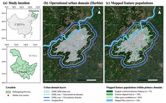
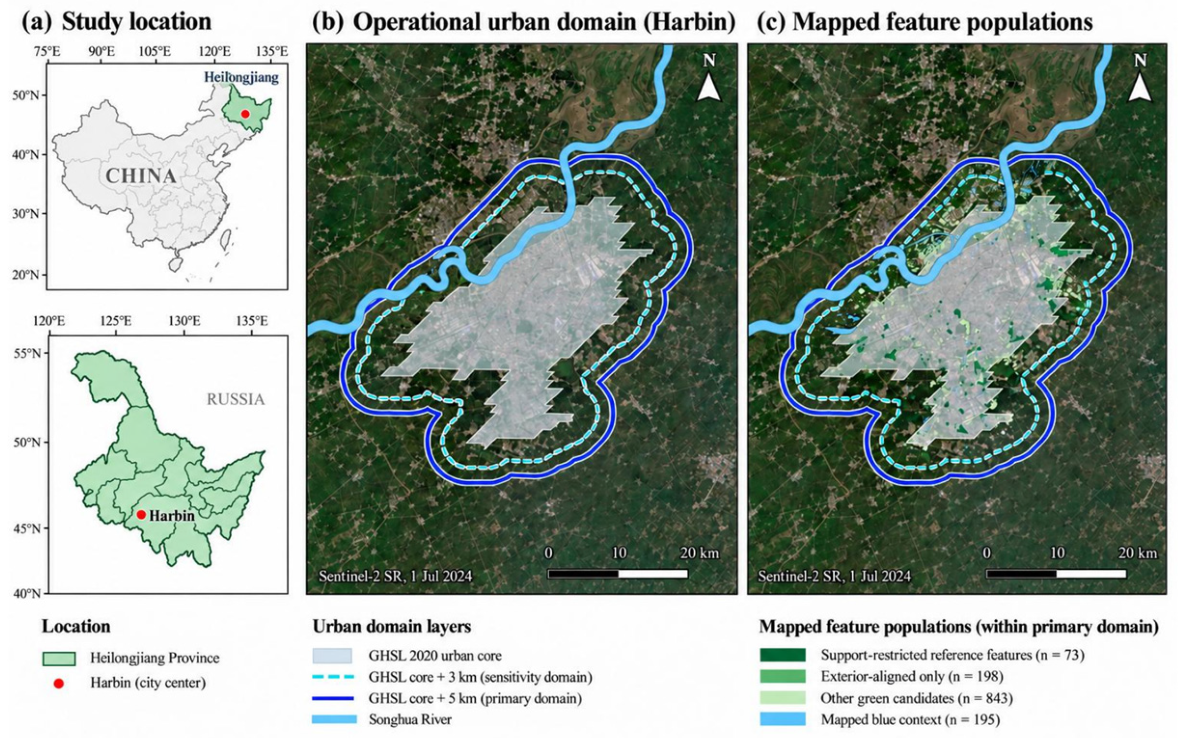
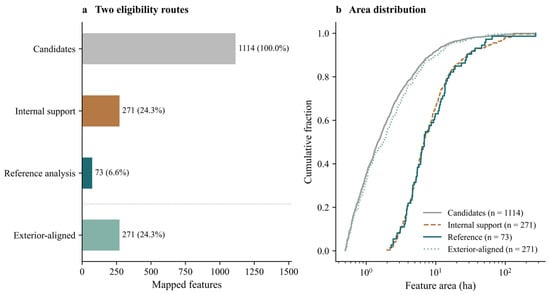
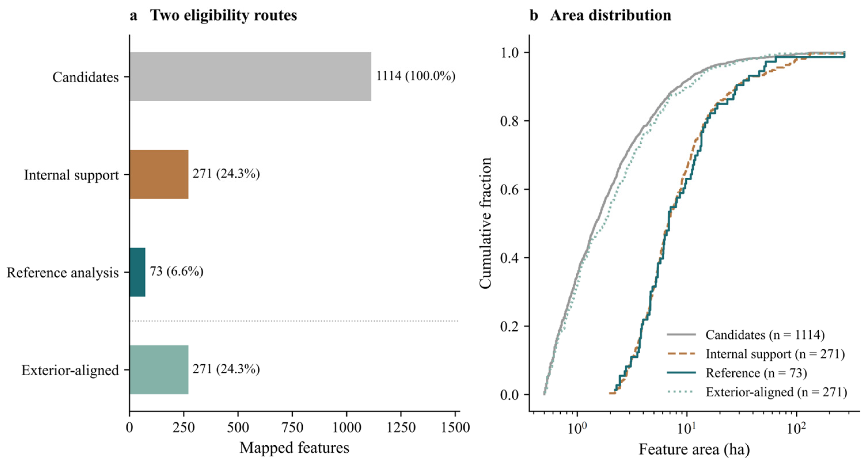
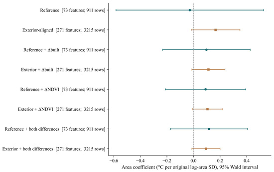
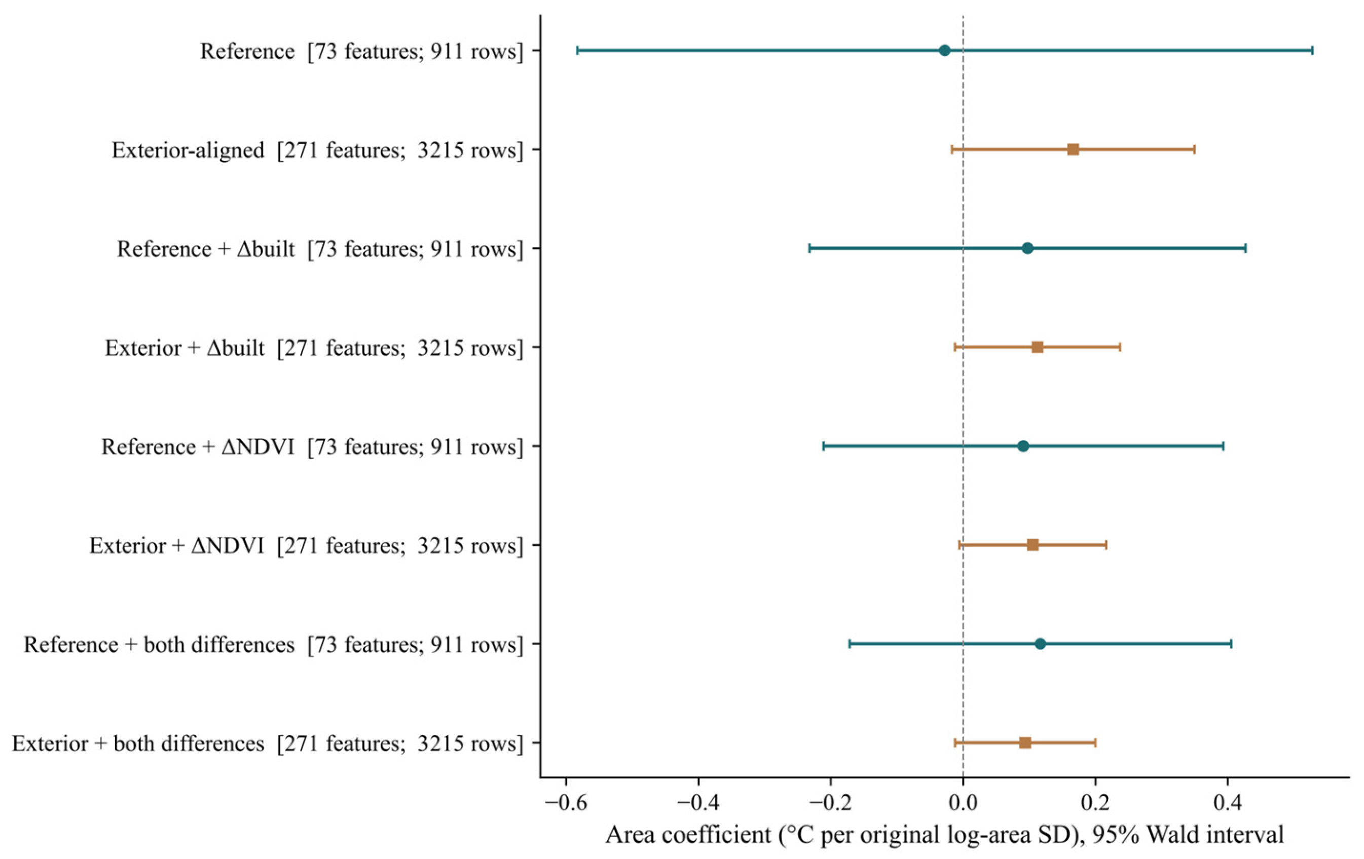
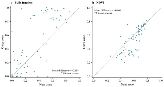
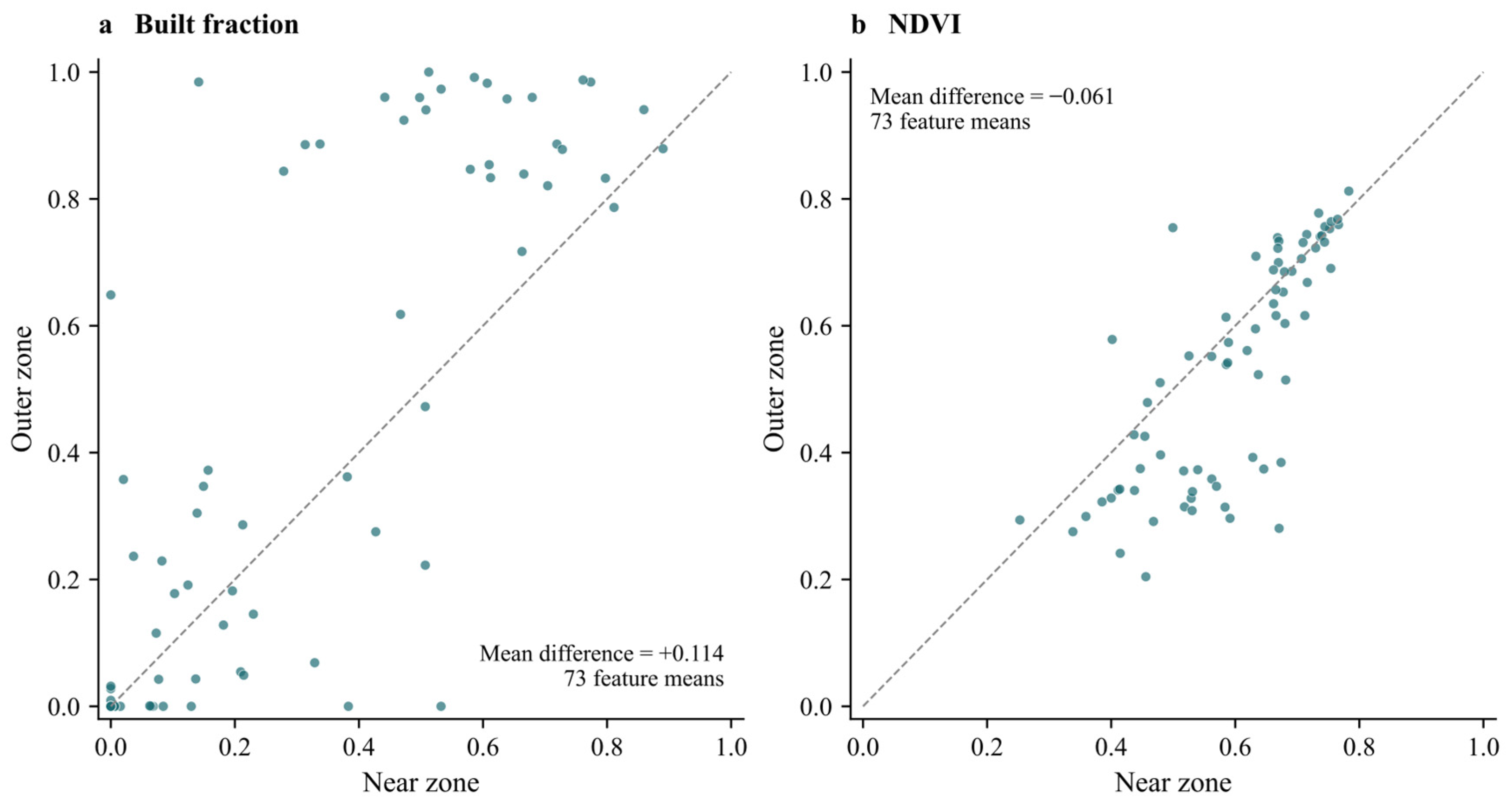
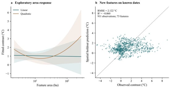
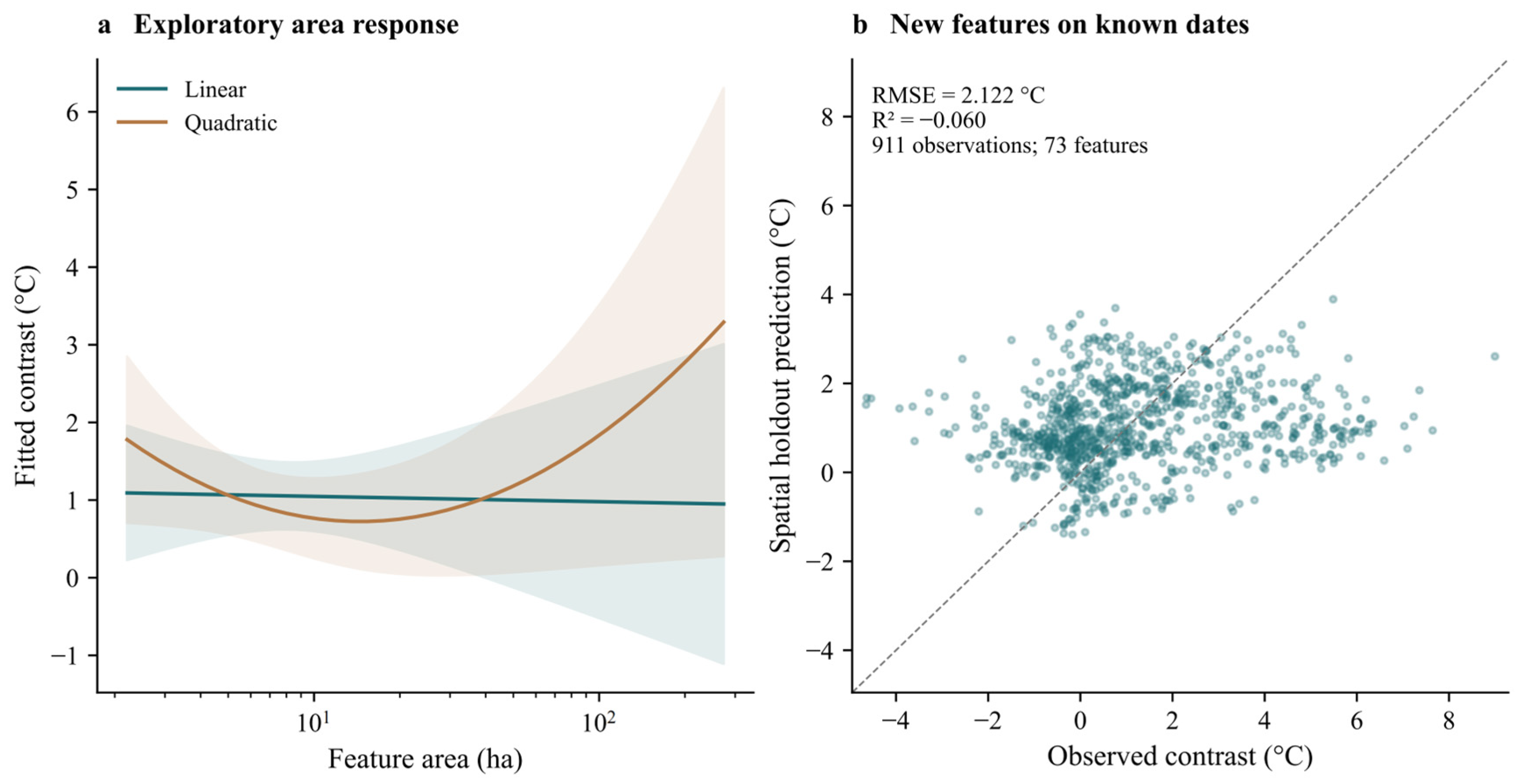

Disclaimer/Publisher’s Note: The statements, opinions and data contained in all publications are solely those of the individual author(s) and contributor(s) and not of MDPI and/or the editor(s). MDPI and/or the editor(s) disclaim responsibility for any injury to people or property resulting from any ideas, methods, instructions or products referred to in the content. |
© 2026 by the authors. Licensee MDPI, Basel, Switzerland. This article is an open access article distributed under the terms and conditions of the Creative Commons Attribution (CC BY) license.