Alleviating Baumol’s Cost Disease with Artificial Intelligence: Mechanisms from an Economic Sustainability Perspective

Abstract

The service sector accounts for a growing share of economic activity, yet relatively slow productivity growth leaves firms facing wage-driven cost pressures that constrain long-term investment. From an economic sustainability perspective, alleviating Baumol’s cost disease can help service firms improve productivity and reduce reliance on additional factor inputs. Drawing on the resource-based view and dynamic capabilities theory, this study applies double machine learning to Chinese A-share-listed service firms from 2011 to 2024 to examine the alleviating effect of artificial intelligence (AI) on Baumol’s cost disease and its potential pathways. Higher AI use intensity is significantly associated with a higher Baumol’s cost disease alleviation indicator (BMR). Greater capital investment efficiency and lower long-term debt financing dependence are two potential pathways, while supplier concentration and growth opportunities positively moderate this relationship. The association is stronger among loss-making firms and firms with greater ownership balance. These findings provide firm-level evidence that AI may help service firms cope with rising wages through productivity growth, supported by more efficient capital allocation and improved financing structures, and contribute to efficiency-driven growth.

1. Introduction

The growing share of services in economic activity is an important feature of structural change, but it also brings a longstanding problem into sharper focus. Productivity in services generally grows more slowly than in manufacturing, while wages in the two sectors tend to move together in an integrated labor market. The resulting gap between wage growth and productivity improvement is the cost disease described by Baumol’s unbalanced-growth model [1]. When efficiency gains cannot absorb wage increases, relatively inflexible costs erode profits and crowd out long-term investment in research and development, data accumulation, and service innovation. Firms may then depend more heavily on additional factor inputs to maintain operations, making the transition from input expansion to efficiency-driven growth difficult. From an economic sustainability perspective, the development of services therefore depends not only on expansion in scale but also on firms’ ability to sustain productivity gains, investment in innovation, and long-term competitiveness as wages rise. Alleviating Baumol’s cost disease is an important part of this transition.

The service sector has become increasingly important to China’s economy. In 2025, services accounted for 57.7% of GDP and contributed 61.4% of national economic growth, while also providing substantial employment support [2]. However, this expansion in scale has not been matched by commensurate efficiency gains. Service-sector labor productivity remains below that of manufacturing, and the longstanding problem of being “large but not strong” has not been fundamentally resolved. Whether firms can absorb wage pressure through better resource allocation and higher productivity thus matters for the efficiency and long-term competitiveness of services, as well as for the broader transition from factor-driven to efficiency-driven growth.

Baumol’s cost disease has been repeatedly documented in macroeconomic and industry data across countries [3,4]. Studies of possible remedies have considered structural change, digital technology, and firm-level technology adoption. At the firm level, AI investment is associated with growth in sales, employment, and product innovation [5]. Experimental evidence from cognitively intensive service tasks shows that generative AI can reduce completion time while improving output quality [6]. Field evidence from customer-service settings likewise documents productivity gains among workers using generative AI [7]. The productivity effects of automation have also received empirical support [8]. Although these studies provide evidence of AI-related efficiency gains, they generally focus on task performance, firm growth, or productivity. Less is known about how firm-level AI use relates to Baumol-type cost pressure, including wage–productivity gaps and unit-labor-cost growth, or about the roles of capital investment efficiency and long-term debt financing dependence.

To address this gap, this study examines whether and how AI use alleviates Baumol’s cost disease among Chinese A-share-listed service firms. It makes three contributions. First, by distinguishing firm-level AI use intensity from general digitalization, it examines the relationship between AI use and cost-disease pressure and extends the firm-level literature on potential remedies. Second, it uses orthogonalization and firm-grouped cross-fitting within a double machine learning framework to reduce regularization and overfitting concerns, with conventional two-way fixed effects as a benchmark. Third, drawing on the resource-based view and dynamic capabilities theory, it investigates capital investment efficiency and long-term debt financing dependence as two potential pathways and discusses their implications for economic sustainability in services. Evidence from Chinese service firms may also inform other emerging economies facing comparable wage–productivity constraints.

2. Theoretical Background and Hypothesis Development

2.1. Direct Effect of AI on Baumol’s Cost Disease in Services

Baumol’s unbalanced-growth model describes how cost disease arises in services [1]. In an integrated labor market, service productivity increases more slowly than manufacturing productivity, but service wages must keep pace with wages in the more progressive sector. The resulting systematic wage–productivity gap pushes up unit labor costs. Two features of services amplify this difficulty. First, service production and consumption often take place at the same time, limiting the decomposition, storage, and scaling of service processes. Second, many activities are unstructured and require workers’ experience, intuition, and contextual judgment, beyond the reach of conventional rule-based automation. Service firms must nevertheless match broader wage increases to retain employees. As the gap between slow productivity growth and increasing wages persists, firms may rely on additional inputs to maintain operations and have less capacity for innovation and continuing efficiency improvements.

The resource-based view helps explain the firm-level origins of this constraint. Firms are heterogeneous combinations of resources, and their competitive advantage depends on the attributes and configuration of those resources [9,10]. Service production relies heavily on labor, whose productivity often grows relatively slowly; simultaneous delivery and non-routine tasks make large efficiency gains difficult to achieve through traditional methods. At the firm level, Baumol’s cost disease may therefore represent a resource-structure trap created by excessive reliance on one productivity-constrained input. The difficulty lies in the concentration of the resource structure rather than necessarily in the quality of labor itself: as wages rise economy-wide, firms have limited alternatives with which to offset the cost pressure. AI may alter this constraint by changing how resources are combined in service delivery. First, real-time interpretation and generative responses can allow some differentiated services to move from one-to-one human delivery toward one-to-many parallel processing, extending service capacity without proportional labor increases. Second, AI can separate certain cognitive tasks from human workflows. Unlike conventional automation, which largely handles repetitive tasks governed by explicit rules, AI can interpret and respond to non-standardized requests, making some cognitive services easier to standardize and scale. Third, AI can reduce the marginal cost of differentiated service provision, enabling firms to serve additional demand with a given resource base and increase output per unit of input.

By processing differentiated demand at scale, separating cognitive tasks from exclusively human workflows, and lowering marginal service costs, AI may relax the limited scalability of many service activities. Firms can generate more output from a given set of inputs, improving total factor productivity (TFP). If service wages increase alongside those in more productive sectors, these efficiency gains can narrow the structural wage–productivity gap. Lower labor requirements per unit of output also reduce unit labor costs relative to what they would otherwise be, helping firms withstand wage pressure. AI thus changes the resource composition of service production and strengthens firms’ capacity to absorb rising wages through productivity rather than continued input accumulation. This transition provides a firm-level basis for economic sustainability in services. Accordingly:

H1. 

Higher AI use intensity significantly alleviates Baumol’s cost disease.

2.2. Capital Investment Efficiency as a Pathway

Baumol’s cost disease reflects both the relatively slow pace of technological progress in services and firms’ difficulty in adjusting factor allocation sufficiently quickly to absorb wage pressure. The resource-based view holds that competitive advantage depends on the effective combination and deployment of heterogeneous resources [11]. Longstanding dependence on labor can create a rigid resource structure in service firms. When wages rise across the labor market, the efficiency of the existing resource mix may deteriorate and cost pressure can accumulate. Whether firms can shift capital away from inefficient uses toward productivity-enhancing investments is therefore important for absorbing higher wages. AI may facilitate this shift from extensive asset expansion toward more efficient investment decisions.

Capital allocation presents a structural challenge for service firms. When business activity expands and operating costs rise, firms may increase their asset holdings in an attempt to compensate for the inseparability and non-storability of service production. Yet resource-allocation efficiency depends more on how assets are combined and used than on the scale of investment alone [11]. Excessive investment in auxiliary assets ties up capital that may not complement core service activities effectively, leading to idle funds, slower turnover, and resource misallocation. Higher asset holdings also increase maintenance and depreciation expenses without necessarily generating corresponding output gains. Under sustained wage pressure, capital committed to inefficient uses crowds out investment that could improve productivity and reinforces existing allocation inefficiencies. Firms consequently have less scope to reallocate resources when costs rise, leaving them more exposed to the productivity constraints underlying Baumol’s cost disease.

AI can improve the information available for investment decisions and thereby reduce distortions associated with conventional investment practices. Capital investment efficiency depends on identifying valuable opportunities under uncertainty and directing limited funds toward projects that improve productivity. Decisions based mainly on managerial experience and restricted information-processing capacity may lead either to excessive investment driven by optimistic expectations or to underinvestment when valuable upgrading opportunities are missed. Both distortions can weaken capital allocation and intensify operating costs as wages rise. AI may help overcome these information frictions through data integration, pattern recognition, and predictive analysis. From the perspective of dynamic capabilities, more accurate demand forecasts and project assessments strengthen firms’ capacity to sense promising opportunities, while better screening and resource coordination help them seize those opportunities, release capital tied up in inefficient projects, and redirect it toward more productive uses.

Improving capital investment efficiency can help service firms absorb the cost pressure arising from higher wages and alleviate Baumol’s cost disease. Releasing capital from inefficient uses may lower fixed operating costs and depreciation burdens, improve the unit cost structure, and reduce the pressure created by rising labor costs. Resources freed through this process can be redirected toward research and innovation, digital infrastructure, and human-capital upgrading, strengthening the basis for sustained productivity improvement. By reallocating capital more effectively, firms may shift away from extensive expansion toward efficiency-driven development. Accordingly:

H2. 

Higher AI use intensity alleviates Baumol’s cost disease through higher capital investment efficiency.

2.3. Long-Term Debt Financing Dependence as a Pathway

Alongside capital investment efficiency, financing-structure adjustment represents a second potential pathway through which AI may alleviate Baumol’s cost disease. Research on resource orchestration emphasizes the fit between organizational conditions and complementary resources [11]. Excessive dependence on long-term debt financing can expose service firms to fixed repayment commitments and financial vulnerability, limiting the resources available for innovation and productivity-enhancing investment. As wages increase, highly leveraged long-term financing structures may make it harder to reallocate funds toward efficiency improvements. Reducing this dependence and restoring financial flexibility can therefore support sustained productivity growth.

Traditional service firms may rely on non-current liabilities to fund expansion and absorb higher operating costs. Heavy dependence on long-term debt increases repayment and refinancing pressure, reduces financial flexibility under rising wages, and may constrain the allocation of resources to more productive activities [12]. When margins are squeezed, cash-flow constraints can further reduce resources for research and efficiency-oriented investment. AI may assist financing adjustments by improving operating efficiency, cash-flow management, and the information environment. Higher operating efficiency can strengthen cash flows, while lower information asymmetry may allow firms to adjust their financing structure at more reasonable costs. From a dynamic-capabilities perspective, these changes can support resource transformation by releasing funds previously tied to debt maintenance and redirecting them toward efficiency-enhancing uses, reducing rigidities and losses arising from excessive long-term debt financing dependence.

Lower dependence on long-term debt financing expands the financial room available to service firms as wages rise. Firms may then direct more resources toward research and development, data capabilities, and human-capital upgrading, creating a reinforcing relationship between efficiency improvements and capability accumulation. Reduced financial vulnerability may also allow firms to maintain productivity-enhancing investment rather than cut it in response to debt-service pressure. Financing-structure optimization can thus ease present cost constraints while providing financial support for future productivity growth. Accordingly:

H3. 

Higher AI use intensity alleviates Baumol’s cost disease through lower long-term debt financing dependence.

2.4. Moderating Effects of Supplier Concentration and Growth Opportunities

The cost-disease-alleviating association with AI is unlikely to be uniform across firms. It can depend on organizational and market conditions. The resource-based view explains why AI may constitute a strategic resource capable of improving efficiency, but it does not fully account for the different outcomes of firms adopting similar technologies. Dynamic capabilities theory offers a complementary explanation by emphasizing firms’ ability to integrate, build, and reconfigure internal and external competences in changing environments [13]. Its microfoundations include sensing opportunities, seizing opportunities, and transforming resources [14]. Whether AI capabilities translate into productivity improvement depends on organizational resource reconfiguration and on the conditions under which firms can sense opportunities, combine complementary assets, and implement new technology. Supplier concentration reflects external collaboration, information acquisition, and resource integration within the supply chain. Growth opportunities capture the incentives to undertake productive technological investment and translate digital resources into efficiency gains. The former is closely related to the external conditions for sensing and seizing opportunities, while the latter concerns incentives for internal resource transformation. Accordingly:

H4. 

The effect of AI use intensity in alleviating Baumol’s cost disease is moderated by supplier concentration and growth opportunities.

Supplier concentration reflects the closeness of a firm’s relationships with its major suppliers and the extent of information exchange. Higher concentration may indicate more stable partnerships and smoother coordination between upstream and downstream operations. Prior research suggests that information sharing along the supply chain can improve inventory management, demand forecasting, and coordinated decisions [15]. Stable supplier relationships can facilitate the practical adoption of AI in procurement planning, inventory scheduling, demand forecasting, and coordination across firms. They may also reduce information errors and coordination costs, allowing service firms to respond more quickly to changes in market demand and adjust resource allocation. From a dynamic capabilities perspective, access to shared supply-chain information can strengthen opportunity sensing by improving the identification of demand changes, while lower coordination costs can facilitate opportunity seizing through the integration of complementary upstream and downstream resources. These conditions may enable firms to translate AI capabilities into productivity gains more effectively, helping absorb wage pressure and strengthening the association between AI use intensity and the alleviation of Baumol’s cost disease. Accordingly:

H4a. 

Supplier concentration positively moderates the effect of AI use intensity in alleviating Baumol’s cost disease.

Growth opportunities reflect capital-market expectations about a firm’s future growth potential and value. Firms with stronger prospects may have greater incentives to use AI for business-process improvement, service innovation, and productivity-enhancing activities. Tobin’s Q provides a conventional proxy for such opportunities. A value above one indicates that the market value of assets exceeds their replacement cost, suggesting scope for profitable investment and expansion [16]. Stronger growth prospects can create both a need for efficiency improvements and favorable conditions for AI deployment. In terms of dynamic capabilities, expectations of higher future returns may encourage firms to transform their resources by reorganizing internal activities and improving production processes. When industry wages and operating costs rise, growth-oriented firms may be more willing to pursue efficiency gains through AI than to rely on extensive increases in conventional inputs. Such proactive adjustment may help translate AI-related technological capacity into higher productivity and strengthen its association with cost-disease alleviation. Accordingly:

H4b. 

Growth opportunities positively moderate the effect of AI use intensity in alleviating Baumol’s cost disease.

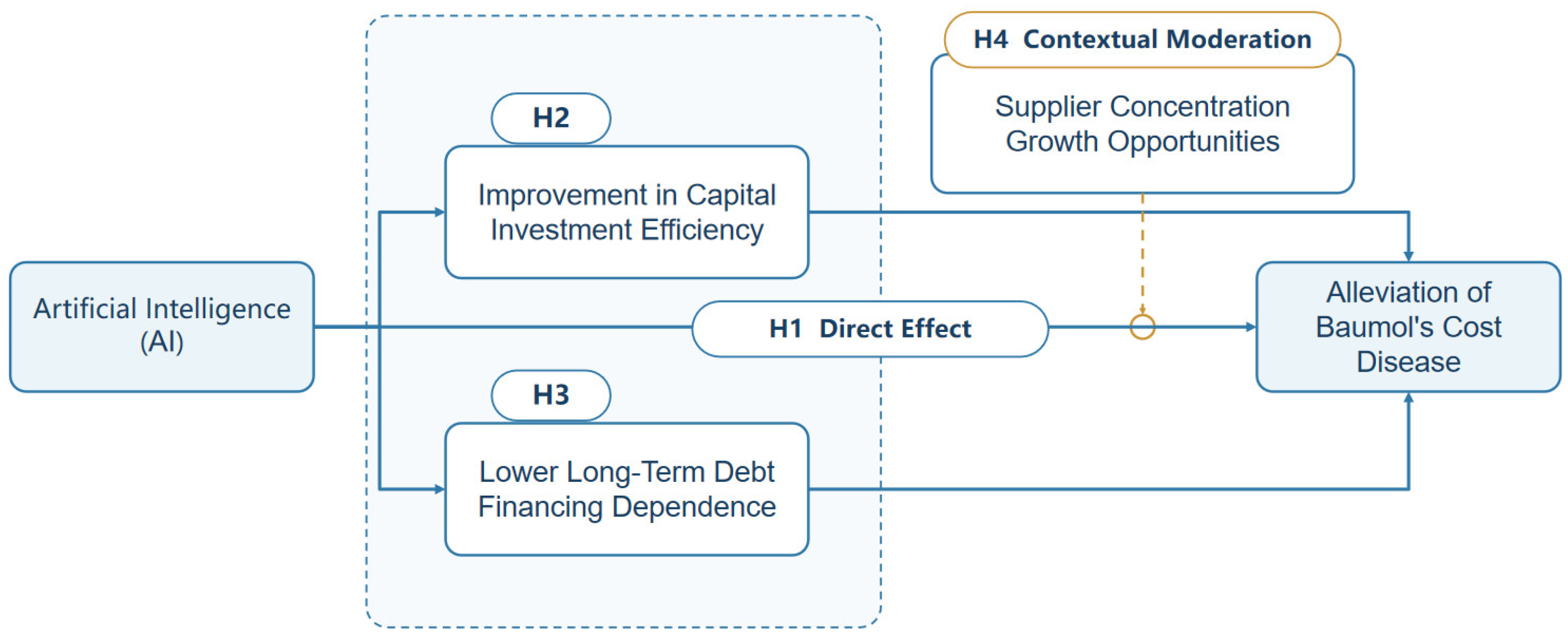
The theoretical framework is presented in Figure 1.

Figure 1. Theoretical framework for AI and Baumol’s cost disease.

3. Research Design

3.1. Data Sources and Sample Selection

3.1.1. Data Sources

The study uses Chinese A-share-listed service firms from 2011 to 2024. Financial information, corporate-governance data, industry classifications, and other firm characteristics were primarily obtained from the China Stock Market and Accounting Research (CSMAR) database. AI use intensity was constructed from the Management Discussion and Analysis (MD&A) sections of annual reports. AI patent data were obtained from the China Research Data Services Platform (CNRDS). The number of prefecture-level-city post offices in 1984, used to construct the instrument, was collected from the China City Statistical Yearbook and related historical materials. Provincial GDP deflators and fixed-asset-investment price indices were used for unit-labor-cost growth and TFP price-deflation sensitivity tests, respectively. These data were obtained from the National Bureau of Statistics of China and provincial statistical materials.

3.1.2. Sample Selection

To construct a consistent estimation sample, we (1) excluded financial, ST, and PT firms; (2) retained listed firms in the service sector; (3) removed observations with missing core variables; (4) retained firms observed for at least two consecutive years; and (5) winsorized continuous variables. The final unbalanced panel contains 9997 firm-year observations for 1241 service firms.

3.2. Variable Definitions

3.2.1. Dependent Variable: Baumol’s Cost Disease Alleviation Indicator (BMR)

A defining feature of Baumol’s cost disease is the failure of productivity improvements to absorb rising wages. Rather than treating total factor productivity (TFP) directly as the conceptual outcome, this study constructs a Baumol’s cost disease alleviation indicator (BMR) using residual-based TFP estimated from a fixed-effects production function. A higher BMR indicates greater output from a given bundle of inputs and a stronger capacity to absorb wage pressure, corresponding to lower cost-disease pressure. The measure is calculated within a Cobb–Douglas production-function framework. Operating revenue represents output (Y), while net fixed assets, employee headcount, and intermediate inputs represent capital (K), labor (L), and intermediate inputs (M), respectively. Intermediate inputs are measured as operating costs plus selling, administrative, and financial expenses, less depreciation and amortization and cash paid to and on behalf of employees. These exclusions avoid double-counting labor expenditure and capital depreciation. After taking natural logarithms, we estimate the following production function:

lnY_it = β₀ + β_KlnK_it + β_LlnL_it + β_MlnM_it + μ_i + λ_t + ε_it

Here, μ_i and λ_t denote firm and year fixed effects, respectively, and ε_it is the idiosyncratic error. We calculate BMR as the log output net of the estimated contributions of capital, labor, and intermediate inputs:

$${\mathrm{BMR}}_{\mathit{it}}=\ln Y_{\mathit{it}}-{\widehat{\beta }}_K\ln K_{\mathit{it}}-{\widehat{\beta }}_L\ln L_{\mathit{it}}-{\widehat{\beta }}_M\ln M_{\mathit{it}}$$

The estimated input elasticities from the fixed-effects production function are 0.0318 for capital, 0.0873 for labor, and 0.8439 for intermediate inputs. The baseline outcome is BMR constructed from the residuals of a fixed-effects production function. For robustness, we recalculate the productivity residuals using ordinary least squares (OLS) and the Levinsohn–Petrin (LP) method to construct alternative BMR measures. Although fixed effects absorb time-invariant firm characteristics, they cannot fully address endogenous input choices responding to time-varying productivity shocks. The LP approach uses intermediate inputs as a proxy for unobserved productivity and mitigates simultaneity bias under assumptions of monotonic input responses and a first-order Markov process for productivity [17]. The identification requirements of proxy-variable estimators have been examined in earlier research [18] and different production-function estimators can yield different productivity residuals [19]. Appendix D therefore further tests whether the BMR estimates depend on accounting definitions, price adjustment, or assumptions of common production technology through four specifications: excluding financial expenses from intermediate inputs, restricting the sample to observations reporting depreciation and amortization, applying price deflators, and combining the financial expense exclusion with price adjustment. These are measurement sensitivities, not a change in the interpretation of BMR as an indicator of cost-disease alleviation. We also examine the wage–productivity gap and cash-compensation unit-labor-cost growth as direct supplementary indicators of cost pressure.

3.2.2. Core Explanatory Variable: AI Use Intensity

We measure firm-level AI use intensity (AI) from the Management Discussion and Analysis (MD&A) sections of listed firms’ annual reports. The total occurrences of the 28 AI-specific terms included in the baseline AI dictionary are normalized by total MD&A text length, scaled by 10,000, and transformed using ln(1 + x). This procedure accounts for differences in disclosure length and reduces skewness. Research on corporate financial text shows that the economic meaning of words depends on context [20]. We therefore distinguish AI-specific technical terms from broader references to digitalization and information technology, reducing noise from an overly inclusive dictionary. The resulting firm-year indicator is used as the main explanatory variable; it measures disclosed AI-related use intensity rather than every aspect of actual deployment.

$${\mathrm{AI}}_{\mathit{it}}=\ln (1+\mathrm{10,000}\times {\displaystyle \frac{{\mathrm{AIFreq}}_{\mathit{it}}}{{\mathrm{MDALength}}_{\mathit{it}}}})$$

Here, AIFreq_it denotes the total occurrences of terms from the baseline AI dictionary in the MD&A section, and MDALength_it denotes the combined length of Chinese and English text in the MD&A section. The baseline and expanded AI dictionaries are reported in Appendix Table A1 and Table A2, respectively. As alternative measures, we use the log-transformed expanded-dictionary term frequency (ln(1 + frequency)) and the cumulative stock of AI invention-patent applications. Because patents capture innovative activity rather than actual deployment intensity, they are used only as an external convergent-validity check of the text-based measure [21]. As a disclosure-based proxy, this measure may not capture unreported AI deployment depth.

3.2.3. Control Variables

Following established empirical practice, the baseline controls are firm size (Size), leverage (Lev), return on assets (ROA), and state ownership (SOE). These variables account for observable firm characteristics relevant to the main relationship. The contemporaneous controls enter the conventional two-way fixed-effects (TWFE) benchmark linearly and enter the prediction equations for both the outcome and the treatment in double machine learning (DML). In the lagged-AI robustness specification, predetermined controls are lagged by one period to reduce concerns about contemporaneous reverse causality.

3.2.4. Pathway Variables

The two pathway variables are capital investment efficiency and long-term debt financing dependence, with detailed definitions in Table 1. Capital investment efficiency is calculated from the residual-based Richardson investment model as the negative absolute value of investment inefficiency [22,23]. Higher values indicate a smaller departure from expected investment and more efficient capital allocation. Long-term debt financing dependence is the ratio of total non-current liabilities to total shareholders’ equity. Larger values represent greater reliance on long-term debt to finance operations and expansion.

Table 1. Variable definitions and measurement.

Variable Type	Variable	Symbol	Definition
Dependent variable	Baumol’s cost disease alleviation indicator	BMR	Indicator constructed from residual-based TFP estimated using a fixed-effects production function; higher values indicate lower cost-disease pressure
Core explanatory variable	AI use intensity	AI	ln [1 + 10,000 × (baseline AI-dictionary term count/MD&A text length)]
Control variable	Firm size	Size	Natural logarithm of total assets
Control variable	Leverage	Lev	Total liabilities divided by total assets
Control variable	Return on assets	ROA	Net income divided by total assets
Control variable	State ownership	SOE	One for state-owned firms and zero otherwise
Pathway variable	Capital investment efficiency	InvestEff	Negative absolute investment inefficiency; higher values indicate more efficient capital allocation
Pathway variable	Long-term debt financing dependence	LTDER	Total non-current liabilities divided by total shareholders’ equity
Moderator	Supplier concentration	SupCon	Purchases from the five largest suppliers as a share of annual total purchases (%); lagged one period
Moderator	Growth opportunities	TobinQ	Lagged Tobin’s Q
Heterogeneity variable	Operating status	Loss	One if net profit is negative and zero otherwise
Heterogeneity variable	Ownership balance	Balance	Combined ownership of the second- through fifth-largest shareholders divided by ownership of the largest shareholder

3.2.5. Moderating Variables

Supplier concentration and growth opportunities are used as moderators, both measured with a one-year lag to reflect predetermined operating conditions and reduce concerns about simultaneous determination. Supplier concentration is the share of total annual purchases accounted for by the five largest suppliers and reflects the concentration of upstream relationships. Growth opportunities are proxied by lagged Tobin’s Q, capturing market expectations about future firm value. Definitions are shown in Table 1. The 2010 data serve only to construct the 2011 lagged measures and do not enter the descriptive statistics or regressions. Moderating effects are estimated in the pooled sample using interactions between AI use intensity and each moderator, with the interaction coefficients indicating the direction and magnitude of moderation.

3.2.6. Heterogeneity Variables

Heterogeneity is examined through pooled-sample interactions for operating status and ownership balance. Operating status is a loss indicator equal to one when net profit is negative and zero otherwise. Ownership balance is measured as the combined equity stakes of the second- through fifth-largest shareholders divided by the stake of the largest shareholder, capturing the extent of checks exerted by other major shareholders. Both definitions appear in Table 1. To address multiple-comparison concerns, the p-values of prespecified interactions are adjusted within their test family using the Benjamini–Hochberg procedure [24].

3.3. Model Specification

3.3.1. Baseline Double Machine Learning Model

To estimate the effect of AI use intensity on Baumol’s cost disease, we use a double machine learning approach. Following the partially linear model of Chernozhukov et al. [25], we specify the following model:

BMR_it = θAI_it + g(X_it) + μ_i + λ_t + ε_it

Here, BMR denotes the Baumol’s cost disease alleviation indicator, AI denotes AI use intensity, and X is the control-variable vector. μ_i and λ_t denote firm and year fixed effects, respectively, g(·) is an unknown function, and ε_it is the error term. Subscripts i and t denote firms and years, respectively. To reduce regularization bias, we use orthogonalization and firm-grouped cross-fitting, with Lasso as the base learner [26]. Firms are partitioned into five folds. The conditional expectations of the outcome and treatment are estimated separately, and the cross-fitted residuals are then used in the orthogonalized regression. The baseline specification controls for Size, Lev, ROA, and SOE. A sensitivity specification additionally includes predetermined controls and their nonlinear transformations and interaction features. The baseline DML and TWFE specifications include firm and year fixed effects, with standard errors clustered at the firm level. Conventional TWFE estimates are reported as a benchmark. Implementation details are provided in Appendix B.

3.3.2. Pathway, Moderation, and Heterogeneity Models

The pathway analysis uses two sets of regressions. First, capital investment efficiency and long-term debt financing dependence are separately regressed on AI use intensity. Second, the relationship between each pathway variable and BMR is estimated, conditioned on AI use intensity. Because the pathway variables and BMR are observed in the same year, these estimates do not meet the requirements for identifying causal mediation. The two steps are therefore interpreted as evidence on potential contemporaneous pathways rather than as a decomposition of indirect causal effects.

Moderation and heterogeneity are estimated in pooled samples through interaction terms. Specifically, the interaction between AI use intensity and a moderator or grouping variable is included alongside the main AI term as a joint treatment variable in the partially linear DML specification:

BMR_it = θ₁AI_it + θ₂(AI_it × Z_it) + h(X_it,Z_it) + μ_i + λ_t + ε_it

Here, the interaction coefficient captures the direction and magnitude of moderation. Compared with separate subgroup regressions, pooled-sample interaction tests preserve statistical power and directly test differences across groups. Since several prespecified interactions are examined, p-values are adjusted within each test family using the Benjamini–Hochberg (BH) procedure to control the false discovery rate [24].

3.4. Descriptive Statistics

Table 2 presents descriptive statistics for the principal variables. AI, BMR, Size, Lev, ROA, and SOE each have 9997 available observations. InvestEff, LTDER, SupCon, and TobinQ have different sample sizes owing to missing financial or disclosure data and the construction of lagged variables. The effective sample size is reported separately for each estimation module, while Appendix C provides details on missing-data treatment and imputation sensitivity analyses.

Table 2. Descriptive statistics.

Variable	Available Observations	Mean	Std. Dev.	Min.	Median	Max.
AI	9997	0.541	0.832	0.000	0.000	3.221
BMR	9997	11.371	1.435	8.272	11.250	15.177
Size	9997	22.431	1.382	19.714	22.247	26.449
Lev	9997	0.456	0.219	0.050	0.447	0.925
ROA	9997	0.025	0.069	−0.287	0.031	0.192
SOE	9997	0.435	0.496	0.000	0.000	1.000
InvestEff	9142	−0.034	0.046	−0.276	−0.019	−0.000
LTDER	9916	0.314	0.483	0.000	0.099	2.221
SupCon	8018	35.567	22.211	5.280	31.000	93.300
TobinQ	9035	1.978	1.314	0.839	1.549	8.311

Notes: Table 2 presents descriptive statistics for the principal variables. AI use intensity, BMR, and the four core controls each have 9997 observations. InvestEff, LTDER, and the two lagged moderators (SupCon and TobinQ) have different available sample sizes because of missing financial or disclosure records and lag construction. Each estimation module reports its actual effective sample. Appendix C documents missing-data treatment and imputation sensitivity analyses.

4. Empirical Results

4.1. Baseline Results: The Direct Effect of AI on Baumol’s Cost Disease

To test H1, we estimate the baseline double machine learning (DML) model and report the conventional two-way fixed-effects (TWFE) result for comparison in Table 3. Column (1) contains the TWFE benchmark and column (2) the main DML estimate. The coefficient on AI use intensity is positive and statistically significant at the 1% level. In column (2), an increase of one standard deviation in AI use intensity (0.832) corresponds to a 0.036-unit higher BMR (0.0429 × 0.832), about 2.5% of the BMR standard deviation (1.435). This positive association is consistent with an alleviation of cost-disease pressure and supports H1. The single-period estimate is modest; although persistent wage pressure and gradual AI adoption make longer-run effects an important question, cumulative effects cannot be quantified from the contemporaneous coefficient alone.

Table 3. Baseline regression results.

Variable	(1) TWFE	(2) DML
AI	0.0420 ***	0.0429 ***
	(0.0123)	(0.0125)
Controls	Yes	Yes
Firm fixed effects	Yes	Yes
Year fixed effects	Yes	Yes
Observations	9997	9997
Firms	1241	1241

Notes: Firm-clustered robust standard errors are reported in parentheses. Column (2) is the DML main specification with five-fold firm-grouped cross-fitting. *** indicates significance at the 1% level.

4.2. Direct Tests of Cost-Disease Pressure

To provide direct supplementary evidence on Baumol’s cost disease, Table 4 examines the wage–productivity gap and unit-labor-cost growth. The DML coefficient on AI use intensity for the wage–productivity gap is −0.0249, significant at the 10% level, indicating a smaller excess of wage growth over productivity growth. For unit-labor-cost growth based on real value added, the contemporaneous and one-year-lagged AI coefficients are −0.0339 and −0.0172, significant at the 1% and 5% levels, respectively. The estimates are consistent with both a current association and a lagged relationship between AI use and slower growth in unit labor costs. A one-standard-deviation increase in AI use intensity is associated with a reduction of approximately 0.028 units in unit-labor-cost growth, in line with the BMR results. The multiple-imputation sensitivity analysis is reported in Appendix C.

Table 4. Direct tests of cost-disease pressure.

Variable	(1) Wage–Productivity Gap	(2) Unit Labor Cost Growth	(3) Unit Labor Cost Growth
AI	−0.0249 *	−0.0339 ***
	(0.0142)	(0.0069)
AI (t − 1)			−0.0172 **
			(0.0073)
Controls	Yes	Yes	Yes
Firm fixed effects	Yes	Yes	Yes
Year fixed effects	Yes	Yes	Yes
Observations	9995	9563	7992
Firms	1241	1230	1097

Notes: All estimates are obtained using DML-Lasso with firm and year fixed effects. Firm-clustered robust standard errors are reported in parentheses. Column (1) uses complete cases for the wage–productivity gap. The imputation sensitivity analysis is reported in Appendix C. Columns (2) and (3) report the results for contemporaneous and one-period-lagged AI, respectively. Financial information from 2010 is used only to construct 2011 growth rates and does not enter the regression. Unit-labor-cost growth is constructed only when cash compensation, value added, and adjacent-year information are available; observations with missing underlying accounting information are not imputed. ***, **, and * indicate significance at the 1%, 5%, and 10% levels, respectively.

In economic terms, a one-standard-deviation increase in AI use intensity is associated with an approximately 0.028-unit decline in unit-labor-cost growth (−0.0339 × 0.832), which is directionally consistent with the baseline BMR evidence.

4.3. Robustness Checks

To assess the robustness of the baseline conclusion, we conduct tests using alternative variables, sample adjustments, model settings, and alternative measures. Results are reported in Table 5, Table 6, Table A5 and Table A10. Table 5 reports the variable-substitution, sample-adjustment, and alternative-measure results. Column (1) uses one-period-lagged AI use intensity and lagged predetermined controls. The coefficient is 0.0314 and significant at the 5% level. Column (2) replaces the baseline AI measure with the natural logarithm of one plus the frequency of terms in the expanded AI dictionary. The estimated coefficient is 0.0303 and significant at the 1% level. Column (3) excludes the 2020–2022 pandemic years, yielding a coefficient of 0.0393 that is significant at the 1% level. Columns (4) and (5) reconstruct BMR using OLS- and LP-based productivity residuals, yielding coefficients of 0.0407 and 0.0434, both significant at the 1% level. Column (6) includes predetermined controls and nonlinear features. The coefficient is 0.0870 and significant at the 5% level. Column (7) replaces the text-based AI-use-intensity measure with the cumulative stock of AI invention-patent applications. The coefficient is 0.0354 and significant at the 5% level. Appendix Table A10 further shows positive DML coefficients under all four alternative BMR constructions. The coefficient is significant at the 5% level when intermediate inputs exclude financial expenses, at the 1% level when only observations with reported depreciation and amortization are retained, and at the 10% level under both the price-deflation and joint-adjustment specifications. These results indicate that the baseline conclusion does not depend on a particular accounting-input definition, price adjustment, or pooled-technology assumption.

Table 5. Robustness checks I: variable substitution, sample adjustment, and alternative measures.

Variable	(1) AI (t − 1)	(2) Expanded AI	(3) Excluding Pandemic	(4) BMR (OLS)	(5) BMR (LP)	(6) Predetermined Controls	(7) Cumulative AI Patent Stock
AI (t − 1)	0.0314 **
	(0.0131)
AI		0.0303 ***	0.0393 ***	0.0407 ***	0.0434 ***	0.0870 **	0.0354 **
		(0.0115)	(0.0141)	(0.0123)	(0.0127)	(0.0432)	(0.0161)
Controls	Yes	Yes	Yes	Yes	Yes	Yes	Yes
Firm fixed effects	Yes	Yes	Yes	Yes	Yes	Yes	Yes
Year fixed effects	Yes	Yes	Yes	Yes	Yes	Yes	Yes
Observations	8335	9997	7191	9997	9997	9997	9995
Firms	1116	1241	1172	1241	1241	1241	1240

Notes: All estimates use DML with five-fold firm-grouped cross-fitting; firm-clustered robust standard errors are reported in parentheses. Column (2) uses ln (1 + expanded-dictionary AI term frequency). Column (6) additionally includes predetermined controls and nonlinear features. Column (7) replaces the text-based AI-use-intensity measure with the cumulative stock of AI invention-patent applications. *** and ** indicate significance at the 1% and 5% levels, respectively.

Table 6. Robustness checks II: alternative learners, cross-fitting folds, and random seeds.

Variable	(1) Ridge	(2) Elastic Net	(3) Ten Folds	(4) Seed 1	(5) Seed 2
AI	0.0427 ***	0.0421 ***	0.0422 ***	0.0418 ***	0.0425 ***
	(0.0124)	(0.0124)	(0.0124)	(0.0124)	(0.0124)
Controls	Yes	Yes	Yes	Yes	Yes
Firm fixed effects	Yes	Yes	Yes	Yes	Yes
Year fixed effects	Yes	Yes	Yes	Yes	Yes
Observations	9997	9997	9997	9997	9997
Firms	1241	1241	1241	1241	1241

Notes: Firm-clustered robust standard errors are reported in parentheses. The direction and statistical significance of the main conclusion remain stable across learners and fold structures. *** indicates significance at the 1% level.

We also vary the DML base learner (ridge and elastic net), the number of cross-fitting folds (10 folds), and the random seed used to split firms. The sign and statistical significance of the core result remain stable. Table 6 reports the results.

4.4. Endogeneity Test

Although the baseline model includes firm and year fixed effects and uses orthogonalization and cross-fitting to reduce sensitivity to functional-form misspecification, reverse causality and omitted variables may still threaten identification. We construct an instrument by interacting the number of post offices in each prefecture-level city in 1984 with the leave-one-out lagged industry mean of AI use intensity. The historical distribution of post offices was shaped largely by central planning rather than current decisions by sample firms. Firm fixed effects absorb time-invariant regional characteristics, while the interaction draws on changes over time in industry AI diffusion.

Table 7 presents the instrumental-variable results. In the first stage, the coefficient of the instrument on AI use intensity is 0.1460, significant at the 1% level. The robust first-stage F-statistic is 176.77 and the partial R² is 0.149. Given the importance of clustered errors and heteroskedasticity for instrument diagnostics, we also report the 5% Anderson–Rubin (AR) confidence set [27,28]. In the second stage, the coefficient on AI use intensity is 0.1640, significant at the 5% level, and the AR 5% confidence set of [0.020, 0.322] excludes zero.

Table 7. Endogeneity test results.

Variable	(1) First Stage	(2) 2SLS
Instrument	0.1460 ***
	(0.0110)
Fitted AI		0.1640 **
		(0.0737)
Controls	Yes	Yes
Firm fixed effects	Yes	Yes
Year fixed effects	Yes	Yes
Robust first-stage F	176.77
Partial R2	0.149
Anderson–Rubin 5% confidence set		[0.020, 0.322]
Observations	9293	9293
Firms	1202	1202

Notes: Robust standard errors, clustered by firm, city, and three-digit industry, are reported in parentheses. Both first-stage and 2SLS regressions control for firm and year fixed effects. *** and ** indicate significance at the 1% and 5% levels, respectively. In the placebo regression, the coefficient of the instrument on one-period-lagged BMR is 0.0195 (p = 0.1463).

The IV coefficient is larger than the baseline DML estimate. We therefore compare TWFE, DML, and 2SLS using identical controls and the same IV-effective sample. The respective estimates are 0.0433, 0.0439, and 0.1640. The first two are close to the baseline DML estimate, suggesting that the larger IV coefficient cannot be explained solely by the sample or control settings. Under the relevant instrumental-variable assumptions, IV estimates may represent a local effect for firms whose AI use responds to the instrument, rather than the full-sample relationship [29]. With heterogeneous treatment effects, a difference between the IV and baseline coefficients does not by itself establish instrument invalidity. Appendix E reports the same-sample comparison, reduced-form results, historical-post-office associations, and first-stage diagnostics.

With respect to the exclusion restriction, historical communication infrastructure may still be related to contemporary productivity through long-run economic development, human-capital accumulation, or digital foundations. In a placebo test using one-period-lagged BMR, the instrument has no significant explanatory power for predetermined productivity (coefficient = 0.0195; p = 0.1463). The conditional cross-sectional association between historical post offices and BMR is also insignificant (coefficient = 0.0211; p = 0.300). These tests can mitigate, but cannot eliminate, concerns about the exclusion restriction. We therefore interpret the IV estimates as conditional supplementary evidence regarding direction rather than as precise estimates of effect magnitude.

5. Further Analyses

5.1. Pathway Associations Through Capital Investment Efficiency and Long-Term Debt Financing Dependence

Table 8 reports the two-step pathway tests for capital investment efficiency and long-term debt financing dependence. In column (1), the coefficient of AI use intensity on capital investment efficiency is 0.0041 and significant at the 1% level. The coefficient of investment efficiency on BMR is 0.5369, also significant at the 1% level, while the same-sample total AI coefficient is 0.0431 and significant at the 1% level. In column (2), AI use intensity has a coefficient of −0.0326 on long-term debt financing dependence. The coefficient of this financing measure on BMR is −0.3393; and the same-sample total AI coefficient is 0.0433. All three estimates are significant at the 1% level. The findings are consistent with H2 and H3, but because these are contemporaneous DML associations, they do not identify causal mediation effects or mediation proportions.

Table 8. Pathway analyses: capital investment efficiency and long-term debt financing dependence.

Variable	(1) InvestEff	(2) LTDER
AI use intensity → pathway variable	0.0041 ***	−0.0326 ***
	(0.0011)	(0.0065)
Pathway variable → BMR	0.5369 ***	−0.3393 ***
	(0.1382)	(0.0348)
Same-sample total effect of AI use intensity	0.0431 ***	0.0433 ***
	(0.0130)	(0.0126)
Controls	Yes	Yes
Firm fixed effects	Yes	Yes
Year fixed effects	Yes	Yes
Observations	9054	9916
Firms	1126	1215

Notes: The estimates use DML-Lasso with firm and year fixed effects. Firm-clustered robust standard errors are reported in parentheses. Long-term debt financing dependence is conceptually related to leverage (Lev), but the variance inflation factors do not indicate severe multicollinearity. It is therefore retained as a financing-structure pathway. *** indicates significance at the 1% level.

In economic terms, a one-standard-deviation increase in AI use intensity is associated with an approximately 0.0034-unit increase in capital investment efficiency (0.0041 × 0.832), corresponding to an indirect-association magnitude of roughly 0.0018 units. It is also associated with an approximately 0.027-unit reduction in long-term debt financing dependence (−0.0326 × 0.832), corresponding to an indirect-association magnitude of roughly 0.0092 units. These quantities describe the economic scale of the two pathway associations.

5.2. Moderating Effects of Supplier Concentration and Growth Opportunities

The association between AI use intensity and BMR may vary with firms’ external and internal conditions. Table 9 examines two moderators. In column (1), the coefficient on AI use intensity interacted with supplier concentration is 0.0465, positive and significant at the 1% level, indicating a stronger AI–BMR relationship at higher supplier concentration. In column (2), the interaction with growth opportunities is 0.0165, positive and significant at the 5% level. These results support H4a and H4b. Both moderators are lagged one period, with 2010 records used only to construct the 2011 lagged variables.

Table 9. Moderating-effect tests.

Variable	(1) SupCon	(2) TobinQ
AI use intensity × moderator	0.0465 ***	0.0165 **
	(0.0099)	(0.0070)
Controls	Yes	Yes
Firm fixed effects	Yes	Yes
Year fixed effects	Yes	Yes
Observations	7998	8942
Firms	1165	1120

Notes: All estimates are DML-Lasso TWFE with firm-clustered robust standard errors in parentheses. The moderators are lagged by one period; 2010 observations are used only to construct 2011 lagged values and do not enter the regressions. *** and ** indicate significance at the 1% and 5% levels, respectively.

Both moderators are standardized before their interactions with AI use intensity are formed. Accordingly, a one-standard-deviation increase in supplier concentration is associated with a 0.0465 increase in the marginal AI coefficient, while the corresponding change for growth opportunities is 0.0165. These coefficients have direct interpretations as moderating associations, not as separate effects of the moderators.

The baseline supplier-concentration measure is the percentage of purchases from the five largest suppliers. To determine whether the moderation result depends on this definition, we also use a procurement-concentration Herfindahl–Hirschman index (HHI) and the largest-supplier purchase share. The interactions remain positive and statistically significant, supporting the robustness of the supplier-concentration result; see Appendix Table A4.

5.3. Heterogeneity Analysis

Table 10 examines between-firm differences using interactions estimated in one pooled sample. Column (1) shows a positive interaction coefficient of 0.0395 for loss-making firms relative to profitable firms, significant at the 5% level. Loss-making firms face more immediate operating constraints and may have stronger incentives to use AI to reduce inefficient investments and improve resource allocation. Column (2) indicates that a one-standard-deviation increase in ownership balance is associated with a 0.0272 increase in the AI coefficient, significant at the 1% level. Greater checks by major shareholders may restrain inefficient investment and facilitate internal resource reallocation. Both heterogeneity interactions remain significant after the Benjamini–Hochberg adjustment reported in Appendix Table A3.

Table 10. Heterogeneity tests.

Variable	(1) Loss	(2) Balance
AI use intensity × group variable	0.0395 **	0.0272 ***
	(0.0155)	(0.0098)
Controls	Yes	Yes
Firm fixed effects	Yes	Yes
Year fixed effects	Yes	Yes
Observations	9997	9916
Firms	1241	1215

Notes: All results are firm-grouped five-fold DML interaction tests with firm-clustered robust standard errors in parentheses. BH-adjusted results for the two heterogeneity comparisons are reported in Appendix Table A3. *** and ** indicate significance at the 1% and 5% levels, respectively.

6. Discussion

6.1. Main Findings and Implications for Economic Sustainability

Using a panel of Chinese A-share-listed service firms from 2011 to 2024, this study employs double machine learning to examine AI use intensity, Baumol-type cost pressure, and potential pathways. AI use intensity is positively associated with BMR, and this result holds across alternative outcomes, the exclusion of the pandemic years, lagged AI specifications, and alternative learners and cross-fitting folds. Direct tests also associate higher AI use intensity with a narrower wage–productivity gap and slower unit-labor-cost growth. The corresponding BMR result is therefore not solely attributable to a particular productivity-based proxy. IV estimates have the same sign but are larger, and are interpreted as conditional supplementary evidence rather than precise estimates of a general causal effect.

The pathway tests suggest two possible ways in which AI use may be related to lower cost-disease pressure. Higher AI use intensity is associated with more efficient capital investment, potentially helping firms identify productive projects and redirect resources from inefficient uses. It is also associated with lower dependence on long-term debt financing, which may improve financial flexibility and preserve resources for productivity-enhancing activity. Taken together, these contemporaneous relationships are consistent with a shift from continued input expansion toward more efficient resource use. Because the variables are measured in the same year, however, the findings do not identify causal mediation.

The moderation results indicate that supply-chain conditions and growth prospects shape the strength of the AI–BMR association. Greater supplier concentration may facilitate information sharing and cross-stage coordination, helping firms apply AI to demand forecasting, procurement planning, and inventory management. Firms with stronger growth opportunities may have greater incentives to undertake process redesign and efficiency-oriented investment using AI. The two moderators thus describe complementary external collaboration and internal incentive conditions under which technological capabilities may become more effective in everyday operations.

The heterogeneity analysis also reveals differences across firms. Loss-making firms experience more acute cost and survival pressures and may therefore have stronger incentives to use AI for resource reallocation. Firms with a greater ownership balance face monitoring by multiple major shareholders, which may constrain inefficient investment and facilitate resource integration. These patterns indicate that sustainable efficiency improvements in services depend not only on technology investment but also on corporate governance and operating conditions.

At a theoretical level, the study describes the firm-level core of Baumol’s cost disease as a resource-structure trap. Service production relies heavily on labor, a relatively productivity-constrained input, while firms have limited alternatives when wages rise. AI may help loosen this trap by processing differentiated demand at scale, separating cognitive tasks, reducing the marginal cost of service delivery, and changing the combination of production inputs. The analysis identifies capital investment efficiency and long-term debt financing dependence as two contemporaneous associational pathways, extending the resource-based view to the service sector and providing firm-level evidence relevant to dynamic capabilities theory. From an economic sustainability perspective, the findings help explain how productivity improvements could reduce reliance on additional inputs and support long-term efficiency-driven growth.

6.2. Policy Implications

First, policy should deepen the practical integration of AI into service-sector operations. In some firms, applications remain concentrated in basic information processing rather than complex judgment and real-time decision-making, limiting the productivity benefits of technology investment. Public support could focus on real business uses—including demand forecasting, resource scheduling, process coordination, and customer service—through demonstration platforms, access to application scenarios, and technology-matching services. Such measures could help firms integrate AI into core operations and increase output per unit of input.

Second, policy should encourage better capital allocation and greater financing resilience. The pathway evidence associates AI use with more efficient investment and reduced reliance on long-term debt financing. Support for digital upgrading and data-resource development could help firms release capital from inefficient uses and redirect existing resources toward productivity-enhancing projects and long-term capabilities. A more developed multi-tier capital market and broader financing channels could also improve debt structure and help service firms maintain productive investment despite wage pressure.

Third, policies could promote supply-chain collaboration and favorable growth conditions. The moderation evidence suggests that supplier concentration and growth opportunities strengthen the AI–BMR relationship. Encouraging stable cooperation with core suppliers, information sharing along the value chain, and coordination across production stages could create conditions in which AI-related efficiency gains are easier to realize. Improving the business environment and innovation infrastructure may also strengthen long-term growth opportunities and firms’ incentives to use AI for process redesign and efficiency upgrading.

Fourth, support should be tailored to firm characteristics rather than applied uniformly. The observed relationship is stronger for loss-making firms and those with greater ownership balance. Firms under acute operating pressure may benefit from targeted digital-transition assistance and technological upgrading services that help reduce costs and improve resource allocation. Where ownership checks and internal governance are weak, better supervision and decision-making procedures could improve the conditions for resource reorganization and the productive use of AI.

Fifth, effective AI implementation requires human capital and organizational support. Embedding AI in service processes depends not only on technology expenditure but also on specialist skills, human–AI coordination, and organizational learning. Regular digital skills training, targeted talent development and recruitment, and access to real application scenarios could improve firms’ capacity for human–AI collaboration, workflow redesign, and digital-resource integration, supporting sustained efficiency improvement.

6.3. Limitations and Future Research

This study has several limitations. First, our text-based measure of AI use intensity is based on annual-report disclosures of AI-related corporate activities rather than direct observations of actual technology adoption. MD&A disclosures may not fully capture the extent to which AI is integrated into firms’ routine operations. Similarly, AI patent applications reflect innovative activity but do not necessarily indicate actual operational deployment. Text-based and patent-based measures are therefore complementary but imperfect proxies for actual AI adoption. Future research could improve measurement accuracy by incorporating firm surveys or direct implementation records. Second, the IV results offer conditional identification support, and the pathway analyses are contemporaneous associations rather than complete causal mediation. Third, the sample is limited to Chinese A-share-listed service firms, so generalization to small and medium-sized firms, unlisted firms, and other institutional settings remains to be tested. Fourth, the direct tests focus on the wage–productivity gap and unit-labor-cost growth. Future work could incorporate service quality, long-term investment, and income distribution. Fifth, we use provincial GDP deflators and fixed-asset-investment price indices in TFP price-sensitivity tests, but firm-level price indices matched to detailed service subsectors remain unavailable. More granular service-price data could improve measurement precision in future research.

Appendix E.1. Same-Sample Comparison of TWFE, DML, and 2SLS

Appendix Table A11 compares TWFE, DML, and 2SLS estimates from the same IV-effective sample of 9293 observations and 1202 firms. All specifications contain the same controls and fixed effects. The TWFE and DML coefficients are 0.0433 and 0.0439, respectively, both significant at the 10% level, whereas the 2SLS coefficient is 0.1640 and significant at the 5% level. The similarity between the first two estimates and the baseline DML result suggests that the larger 2SLS estimate is not simply attributable to sample composition or control choices; the underlying estimands may differ.

Table A11. Same-sample comparison of TWFE, DML, and 2SLS.

Variable	(1) TWFE	(2) DML-Lasso TWFE	(3) 2SLS
AI	0.0433 *	0.0439 *	0.1640 **
	(0.0231)	(0.0232)	(0.0737)
Controls	Yes	Yes	Yes
Firm fixed effects	Yes	Yes	Yes
Year fixed effects	Yes	Yes	Yes
Observations	9293	9293	9293
Firms	1202	1202	1202

Notes: All columns use the same IV-effective sample and identical control variables and firm and year fixed effects. Standard errors are clustered by firm, city, and three-digit industry. ** and * indicate significance at the 5% and 10% levels, respectively.

Table A11. Same-sample comparison of TWFE, DML, and 2SLS.

Variable	(1) TWFE	(2) DML-Lasso TWFE	(3) 2SLS
AI	0.0433 *	0.0439 *	0.1640 **
	(0.0231)	(0.0232)	(0.0737)
Controls	Yes	Yes	Yes
Firm fixed effects	Yes	Yes	Yes
Year fixed effects	Yes	Yes	Yes
Observations	9293	9293	9293
Firms	1202	1202	1202

Notes: All columns use the same IV-effective sample and identical control variables and firm and year fixed effects. Standard errors are clustered by firm, city, and three-digit industry. ** and * indicate significance at the 5% and 10% levels, respectively.

Appendix E.2. First Stage, Reduced Form, and 2SLS

Appendix Table A12 reports three links in the IV estimation. First, the coefficient of the instrument on AI use intensity is 0.1460, significant at the 1% level. Second, the reduced-form coefficient of the instrument on BMR is 0.0239, significant at the 5% level, showing a conditional association between the instrument and the outcome. Third, the 2SLS coefficient of AI use intensity on BMR is 0.1640, also significant at the 5% level. These results are interpreted subject to the underlying IV assumptions.

Table A12. First stage, reduced form, and 2SLS.

Variable	(1) First Stage	(2) Reduced Form	(3) 2SLS
Instrument	0.1460 ***	0.0239 **
	(0.0110)	(0.0102)
Fitted AI			0.1640 **
			(0.0737)
Controls	Yes	Yes	Yes
Firm fixed effects	Yes	Yes	Yes
Year fixed effects	Yes	Yes	Yes
Observations	9293	9293	9293
Firms	1202	1202	1202

Notes: Robust standard errors, clustered by firm, city, and three-digit industry, are reported in parentheses. The first-stage, reduced-form, and 2SLS regressions all include firm and year fixed effects. *** and ** indicate significance at the 1% and 5% levels, respectively.

Table A12. First stage, reduced form, and 2SLS.

Variable	(1) First Stage	(2) Reduced Form	(3) 2SLS
Instrument	0.1460 ***	0.0239 **
	(0.0110)	(0.0102)
Fitted AI			0.1640 **
			(0.0737)
Controls	Yes	Yes	Yes
Firm fixed effects	Yes	Yes	Yes
Year fixed effects	Yes	Yes	Yes
Observations	9293	9293	9293
Firms	1202	1202	1202

Notes: Robust standard errors, clustered by firm, city, and three-digit industry, are reported in parentheses. The first-stage, reduced-form, and 2SLS regressions all include firm and year fixed effects. *** and ** indicate significance at the 1% and 5% levels, respectively.

Appendix E.3. First-Stage Diagnostics

Appendix Table A13 reports first-stage diagnostics. The robust F-statistic is 176.77, well above commonly used weak-instrument benchmarks, and the partial R² is 0.149, indicating substantial explanatory power for AI use intensity.

Table A13. First-stage diagnostics.

Statistic	Value
Observations	9293
Firms	1202
Cities	112
Three-digit industries	29
Partial R2	0.149
Robust first-stage t-statistic	13.30
Robust first-stage F-statistic	176.77
First-stage p-value	<0.001

Notes: Standard errors are clustered by firm, city, and three-digit industry.

Table A13. First-stage diagnostics.

Statistic	Value
Observations	9293
Firms	1202
Cities	112
Three-digit industries	29
Partial R2	0.149
Robust first-stage t-statistic	13.30
Robust first-stage F-statistic	176.77
First-stage p-value	<0.001

Notes: Standard errors are clustered by firm, city, and three-digit industry.

Appendix E.4. Direct Historical-Post-Office Association and Placebo Test

Appendix Table A14 reports the conditional cross-sectional relationship between historical post-office numbers and BMR and a placebo test using one-period-lagged BMR. Historical post-office counts do not vary over time within firms and are therefore absorbed by firm fixed effects; column (1) includes year fixed effects and controls instead. The coefficient on historical post-office counts is 0.0211 (p = 0.300). The placebo coefficient for the instrument on lagged BMR is 0.0195 (p = 0.1463). Neither is statistically significant. These diagnostics are descriptive checks on the exclusion restriction, not proof that it holds.

Table A14. Direct historical-post-office association and placebo test.

Variable	(1) Direct Historical-Post- Office Association	(2) Placebo Test
Historical post-office count	0.0211
	(0.0199)
Instrument (Z)		0.0195
		(0.0130)
Controls	Yes	Yes
Year fixed effects	Yes	Yes
Firm fixed effects	No	Yes
Observations	9293	8113
Firms	1202	1199

Notes: Because historical post-office counts do not vary within firms, column (1) cannot be estimated with firm fixed effects; it therefore includes the control variables and year fixed effects only. Column (2) uses one-period-lagged BMR as the outcome. Standard errors are clustered by firm, city, and three-digit industry.

Table A14. Direct historical-post-office association and placebo test.

Variable	(1) Direct Historical-Post- Office Association	(2) Placebo Test
Historical post-office count	0.0211
	(0.0199)
Instrument (Z)		0.0195
		(0.0130)
Controls	Yes	Yes
Year fixed effects	Yes	Yes
Firm fixed effects	No	Yes
Observations	9293	8113
Firms	1202	1199

Notes: Because historical post-office counts do not vary within firms, column (1) cannot be estimated with firm fixed effects; it therefore includes the control variables and year fixed effects only. Column (2) uses one-period-lagged BMR as the outcome. Standard errors are clustered by firm, city, and three-digit industry.

References

- Baumol, W.J. Macroeconomics of unbalanced growth: The anatomy of urban crisis. Am. Econ. Rev. 1967, 57, 415–426. [Google Scholar]
- Peng, Y. Service Economy Maintained Steady Growth and Transformation Upgrading Accelerated in 2025. National Bureau of Statistics of China. 2026. Available online: https://www.stats.gov.cn/sj/zxfbhjd/202601/t20260119_1962335.html (accessed on 8 October 2026).
- Nordhaus, W.D. Baumol’s diseases: A macroeconomic perspective. B.E. J. Macroecon. 2008, 8, 1–39. [Google Scholar] [CrossRef] [Scilit]
- Hartwig, J. Testing the Baumol–Nordhaus model with EU KLEMS data. Rev. Income Wealth 2011, 57, 471–489. [Google Scholar] [CrossRef] [Scilit]
- Babina, T.; Fedyk, A.; He, A.X.; Hodson, J. Artificial intelligence, firm growth, and product innovation. J. Financ. Econ. 2024, 151, 103745. [Google Scholar] [CrossRef] [Scilit]
- Noy, S.; Zhang, W. Experimental evidence on the productivity effects of generative artificial intelligence. Science 2023, 381, 187–192. [Google Scholar] [CrossRef] [Scilit] [PubMed]
- Brynjolfsson, E.; Li, D.; Raymond, L. Generative AI at work. Q. J. Econ. 2025, 140, 889–942. [Google Scholar] [CrossRef] [Scilit]
- Graetz, G.; Michaels, G. Robots at work. Rev. Econ. Stat. 2018, 100, 753–768. [Google Scholar] [CrossRef] [Scilit]
- Wernerfelt, B. A resource-based view of the firm. Strateg. Manag. J. 1984, 5, 171–180. [Google Scholar] [CrossRef] [Scilit]
- Barney, J. Firm resources and sustained competitive advantage. J. Manag. 1991, 17, 99–120. [Google Scholar] [CrossRef] [Scilit]
- Sirmon, D.G.; Hitt, M.A.; Ireland, R.D. Managing firm resources in dynamic environments to create value: Looking inside the black box. Acad. Manag. Rev. 2007, 32, 273–292. [Google Scholar] [CrossRef] [Scilit]
- Gamba, A.; Triantis, A. The value of financial flexibility. J. Financ. 2008, 63, 2263–2296. [Google Scholar] [CrossRef] [Scilit]
- Teece, D.J.; Pisano, G.; Shuen, A. Dynamic capabilities and strategic management. Strateg. Manag. J. 1997, 18, 509–533. [Google Scholar] [CrossRef] [Scilit]
- Teece, D.J. Explicating dynamic capabilities: The nature and microfoundations of (sustainable) enterprise performance. Strateg. Manag. J. 2007, 28, 1319–1350. [Google Scholar] [CrossRef] [Scilit]
- Cachon, G.P.; Fisher, M. Supply chain inventory management and the value of shared information. Manag. Sci. 2000, 46, 1032–1048. [Google Scholar] [CrossRef] [Scilit]
- Tobin, J. A general equilibrium approach to monetary theory. J. Money Credit Bank. 1969, 1, 15–29. [Google Scholar]
- Levinsohn, J.; Petrin, A. Estimating production functions using inputs to control for unobservables. Rev. Econ. Stud. 2003, 70, 317–341. [Google Scholar] [CrossRef] [Scilit]
- Ackerberg, D.A.; Caves, K.; Frazer, G. Identification properties of recent production function estimators. Econometrica 2015, 83, 2411–2451. [Google Scholar] [CrossRef] [Scilit]
- Lu, X.; Lian, Y. Estimation of total factor productivity in Chinese industrial enterprises: 1999–2007. China Econ. Q. 2012, 11, 541–558. (In Chinese) [Google Scholar] [CrossRef]
- Loughran, T.; McDonald, B. When is a liability not a liability? Textual analysis, dictionaries, and 10-Ks. J. Financ. 2011, 66, 35–65. [Google Scholar] [CrossRef] [Scilit]
- Griliches, Z. Patent statistics as economic indicators: A survey. J. Econ. Lit. 1990, 28, 1661–1707. [Google Scholar]
- Richardson, S. Over-investment of free cash flow. Rev. Account. Stud. 2006, 11, 159–189. [Google Scholar] [CrossRef] [Scilit]
- Biddle, G.C.; Hilary, G.; Verdi, R.S. How does financial reporting quality relate to investment efficiency? J. Account. Econ. 2009, 48, 112–131. [Google Scholar] [CrossRef] [Scilit]
- Benjamini, Y.; Hochberg, Y. Controlling the false discovery rate: A practical and powerful approach to multiple testing. J. R. Stat. Soc. Ser. B 1995, 57, 289–300. [Google Scholar] [CrossRef] [Scilit]
- Chernozhukov, V.; Chetverikov, D.; Demirer, M.; Duflo, E.; Hansen, C.; Newey, W.; Robins, J. Double/debiased machine learning for treatment and structural parameters. Econom. J. 2018, 21, C1–C68. [Google Scholar] [CrossRef] [Scilit]
- Friedman, J.H.; Hastie, T.; Tibshirani, R. Regularization paths for generalized linear models via coordinate descent. J. Stat. Softw. 2010, 33, 1–22. [Google Scholar] [CrossRef] [Scilit]
- Montiel Olea, J.L.; Pflueger, C.E. A robust test for weak instruments. J. Bus. Econ. Stat. 2013, 31, 358–369. [Google Scholar] [CrossRef] [Scilit]
- Anderson, T.W.; Rubin, H. Estimation of the parameters of a single equation in a complete system of stochastic equations. Ann. Math. Stat. 1949, 20, 46–63. [Google Scholar] [CrossRef] [Scilit]
- Imbens, G.W.; Angrist, J.D. Identification and estimation of local average treatment effects. Econometrica 1994, 62, 467–475. [Google Scholar] [CrossRef] [Scilit]
- van Buuren, S. Flexible Imputation of Missing Data, 2nd ed.; Chapman & Hall/CRC: Boca Raton, FL, USA, 2018. [Google Scholar]
- Rubin, D.B. Multiple Imputation for Nonresponse in Surveys; John Wiley & Sons: New York, NY, USA, 1987. [Google Scholar]
Disclaimer/Publisher’s Note: The statements, opinions and data contained in all publications are solely those of the individual author(s) and contributor(s) and not of MDPI and/or the editor(s). MDPI and/or the editor(s) disclaim responsibility for any injury to people or property resulting from any ideas, methods, instructions or products referred to in the content. |
© 2026 by the authors. Licensee MDPI, Basel, Switzerland. This article is an open access article distributed under the terms and conditions of the Creative Commons Attribution (CC BY) license.