


Abstract
Rapid urbanization and intensifying thermal stress pose challenges to urban livability, climate resilience, and sustainable development. However, studies overlook the seasonal nonlinearity and spatial non-stationarity of urban thermal comfort and its driving factors, constraining seasonally differentiated, climate-adaptive planning strategies. Taking central Tianjin, China, as a case study, this research integrates a geographically weighted XGBoost model with shapley additive explanations to disentangle the seasonal and spatial differentiation, nonlinear relationships, and conditional interaction patterns of the Universal Thermal Climate Index (UTCI). Results indicate: (1) UTCI exhibits seasonal differences in spatial thermal gradients, with relatively high values concentrated in central and northern-central areas; (2) driver contributions shift across seasons, with evapotranspiration leading in summer, digital elevation model in autumn, and building density in winter, while landscape composition contributes most strongly in winter; (3) candidate nonlinear breakpoints include winter sky view factor (0.683; 95% interval 0.662–0.752) and water patch density (15.6 patches/100 ha; 13–17.8); (4) conditional interactions vary seasonally, involving environmental–terrain combinations in summer and building-morphology–landscape combinations in winter. These findings reveal season-specific thermal comfort associations, providing quantitative evidence for translating nonlinear relationships and spatial heterogeneity into climate-adaptive urban design. This supports targeted thermal-environment interventions for urban resilience and sustainability.
1. Introduction
Global warming and rapid urbanization have intensified the Urban Heat Island (UHI) effect in high-density cities [1,2], exacerbating outdoor thermal comfort issues and making the precise analysis of thermal comfort a critical bridge for mitigating public health risks in sustainable urban development [3]. While traditional field measurement studies provide localized data [4], faced with the holistic complexity of the urban environment, research is increasingly shifting towards large-scale spatial analysis. To accurately evaluate the urban thermal environment, indicator systems have evolved from single physical parameters, such as Land Surface Temperature (LST), to comprehensive physiological indices like the Universal Thermal Climate Index (UTCI).
Existing outdoor thermal comfort studies cover a variety of assessment methods from local to macro-urban scales, yet each method possesses specific applicability limitations regarding data acquisition and indicator representation. At the local scale, existing studies typically obtain high-precision assessments at specific time points through in situ measurements, rendering cross-temporal and seasonal assessments challenging. At the urban scale, most studies primarily utilize satellite inversion or weather station data, relying on LST or air temperature (AT) as proxy indicators for the outdoor thermal environment [5,6]. Because thermal stress is governed by more than temperature alone, reliance on single parameters such as LST may lead to incomplete or biased assessments of outdoor thermal conditions [7,8]. To overcome this, the Universal Thermal Climate Index (UTCI) is widely adopted [9,10], as it comprehensively integrates air temperature, humidity, wind speed, and radiation into a single biometeorological model to measure dynamic human physiological responses across diverse climate zones [11,12].
The seasonal and spatial differentiation of urban outdoor thermal comfort is associated with multidimensional influencing factors, including topographic features, landscape composition and pattern, environmental conditions, building morphology, and socio-economic characteristics [13,14]. Topographic features like elevation and Aspect alter local airflow and radiation budgets [15,16], while landscape elements and surface attributes, such as water bodies, vegetation, and high-albedo materials, regulate temperatures through latent heat fluxes and reduced heat storage [17,18]. Furthermore, three-dimensional building morphology alters street canyon radiation dissipation and wind attenuation [19,20], while socio-economic characteristics may be associated with differences in human activity intensity and thermal exposure [21,22]. Collectively, these multidimensional factors are associated with complex urban microclimatic responses [23].
Although UTCI establishes theoretical global thermal-stress categories, research indicates that the actual neutral range of thermal comfort can be influenced by seasonal climate memory and psychological expectations [24]. Empirical studies in the Mediterranean and Central Europe have reported seasonal asymmetry and hysteresis in thermal comfort responses, indicating that residents may provide different thermal evaluations across seasons even under comparable UTCI conditions [25,26].
Existing studies are concentrated at either macro-urban/regional scales or micro-scale settings, leaving a clear gap at intermediate spatial scales. At macro-urban and regional scales, studies mainly reveal spatial patterns of thermal stress under broad climate backgrounds and their statistical associations with land cover [27,28]. UTCI is primarily applied to assess climate change trends, extreme heatwave risks, and biometeorological impacts of the UHI effect. Relevant works rely on meteorological station data or mesoscale weather models to map the geographic distribution of thermal stress, aiming to establish quantitative relationships between thermal comfort and macro-climate zones or land cover types [29,30]. While providing effective macro-warnings, the coarse grid resolution of such studies fails to capture specific disturbances of buildings on the wind-thermal environment, making them unable to offer direct guidance for refined urban design. Conversely, at the micro-human-centric scale, research focuses on verifying the improvement effects of specific microclimate adaptive design strategies. Here, UTCI serves as a core dependent variable to test micro-renewal strategies, shrinking the scope to single points or lines. The extensive literature discusses the instantaneous effects of street tree shading, permeable pavements, or street canyon Aspect ratios [31,32]. While highly precise, these studies often have limited ability to capture the spatial continuity and interactions of climatic processes across groups of buildings. Consequently, a gap remains in characterizing within-city spatial variation while integrating finer-resolution explanatory information. Existing macro models have limited spatial detail, while micro-scale measurements have limited areal coverage. The present study addresses this gap through intra-urban gridded analysis on the native nominal 1 km UTCI grid, with finer-resolution explanatory variables aggregated to the native UTCI cells before modeling.
Methodologically, characterizing these within-city spatial associations requires handling complex spatial non-stationarity and nonlinear threshold responses [33,34]. To better address these spatial and methodological gaps [35], this study adopts the Geographically Weighted XGBoost (GW-XGBoost) model to capture spatial heterogeneity and nonlinear relationships among driving factors [36,37]. Furthermore, to overcome the inherent “black-box” opacity of complex machine learning models, GW-XGBoost is paired with the SHAP (SHapley Additive exPlanations) framework. This combined approach provides feature attribution [38], supports the quantitative identification of candidate nonlinear breakpoints [39], and characterizes conditional interaction patterns among built-environment factors [40].
Existing studies rarely systematically explore the seasonal spatial differentiation of UTCI within cities, particularly lacking quantitative analysis of spatial non-stationarity and nonlinear threshold effects. To bridge this gap, taking the central urban area of Tianjin as a case study, this research utilizes the GW-XGBoost model and SHAP interpretability analysis to systematically address the following scientific questions: Under different seasonal climatic backgrounds, what seasonally varying spatial patterns do multidimensional influencing factors exhibit in their associations with thermal comfort? How can the limitations of single macro-surface temperature representation be overcome to characterize the spatial heterogeneity of UTCI at its native nominal 1 km grid while integrating finer-resolution explanatory information? How can candidate nonlinear breakpoints, marginal relationships, and interaction patterns be quantitatively characterized? This study aims to provide a quantitative basis for seasonally differentiated and spatially targeted urban thermal-environment interventions by quantifying candidate nonlinear breakpoints, spatially varying contributions of driving factors, and conditional interaction patterns among key factors. By translating these findings into climate-adaptive planning guidance, the study seeks to support more resilient, livable, and sustainable urban development under increasing climate and urbanization pressures. Such translation requires rigorous spatial validation [41] and careful consideration of the transferability of planning implications [42].
2. Data and Methods
2.1. Study Area
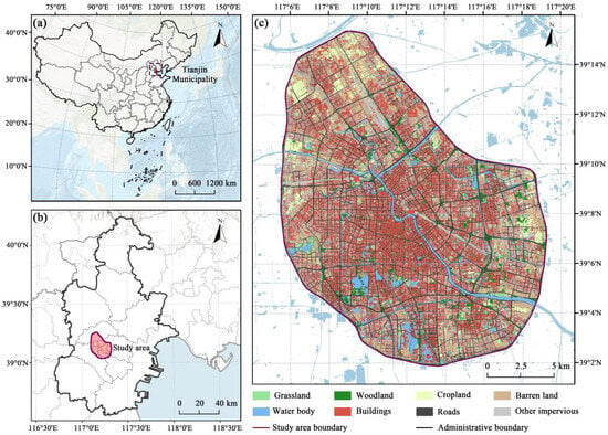
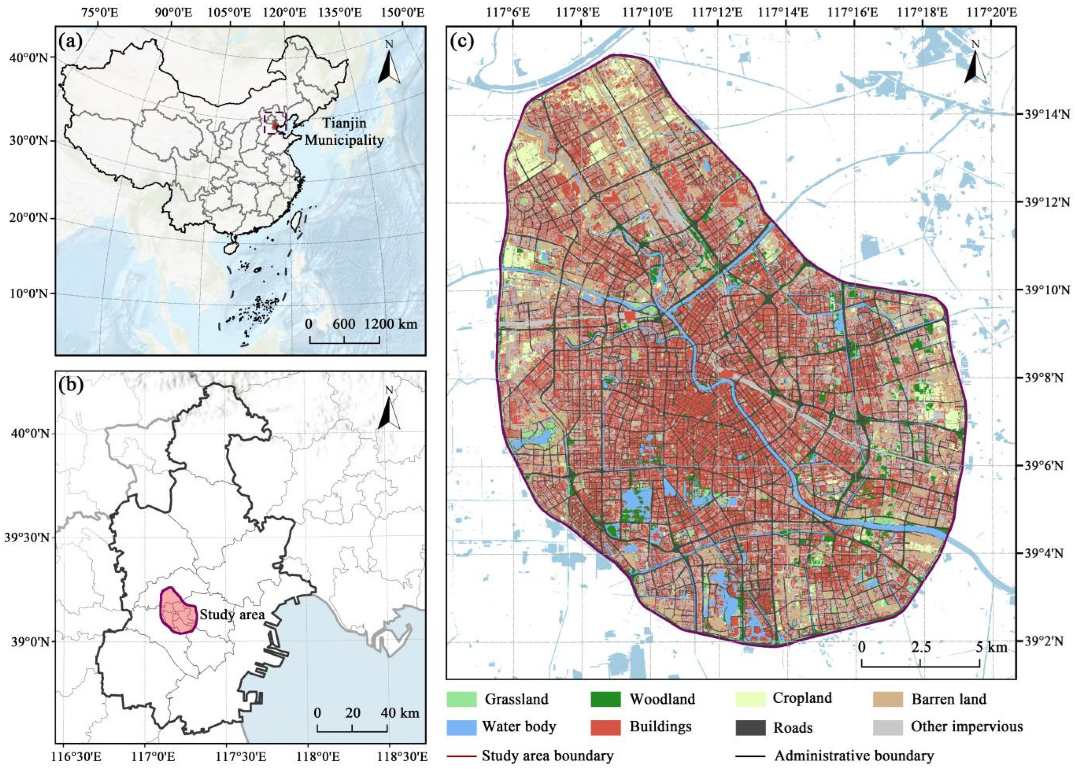
This study focuses on the central urban area of Tianjin, geographically defined by the Outer Ring Road. As a major coastal city in northern China, the study area covers approximately 374 km2 (Figure 1). Located in the northeastern North China Plain, the region is characterized by flat terrain and high urbanization, exhibiting a monocentric, high-density spatial structure expanding concentrically along the Hai River axis. As a typical temperate semi-humid continental monsoon climate zone (Köppen classification: Dwa), Tianjin is controlled by the East Asian monsoon circulation and exhibits pronounced seasonal climatic contrasts. In summer, under the influence of the subtropical high, Tianjin is typically hot, rainy, and humid, with frequent heatwave conditions. In winter, the Mongolian-Siberian high produces cold and dry conditions with prevailing northwesterly winds. The pronounced contrast between hot-humid summers and cold-dry winters provides a suitable climatic setting for examining seasonal differences in urban thermal comfort.
Figure 1.
Location of study area. (a) location of Tianjin in China; (b) location of the study area in Tianjin; (c) land cover of the study area.
2.2. Data and Preprocessing
The primary target variable for this study is thermal comfort, derived from the GloUTCI-M dataset (Table 1). To mitigate the noise from single-month meteorological fluctuations and characterize seasonal thermal regimes, we performed seasonal aggregation on monthly gridded estimates for March 2021–February 2022. By calculating seasonal averages, we generated UTCI raster images that reflect seasonal thermal-environment conditions. Spring, summer and autumn comprise March–May, June–August and September–November 2021, respectively; winter comprises December 2021–February 2022. The product represents its daytime sampling convention (approximately 11:00–14:00 local time), rather than all-day exposure. UTCI retains its original geographic grid (nominally 1 km).
Table 1.
Data sources.
To construct the set of explanatory variables, we integrated multi-source remote sensing and geographic data. First, regarding surface biophysical attributes, Landsat-8 OLI/TIRS images were acquired via the USGS EarthExplorer platform (United States Geological Survey, Reston, VA, USA). Following radiometric calibration and atmospheric correction, cloud-free composite images were generated to retrieve NDVI, surface Albedo, and water proportion. Second, to capture fine-scale landscape patterns, we used the supplied EcoVision-derived land cover map. These data were aggregated to extract the Landscape Shape Index (LSI), Aggregation Index (AI), and Patch Density (PD) for various land use types. Specifically, to clarify the EcoVision classifications within the high-intensity urban core, variables such as Shrub Patch Density (PD_Shrub) and the Landscape Shape Index of unbuilt bare surfaces (LSI_Soil) were extracted, retaining descriptors derived from the supplied polygons for subsequent area-weighted aggregation. Finally, to account for three-dimensional urban morphology and topography, vector building data were rasterized to compute Building Height (BH), BD, and Floor Area Ratio (FAR), while topographic features, including Slope, Aspect, and Topographic Wetness Index (TWI), were derived from ASTER GDEM V2 data.
To ensure spatial consistency, all explanatory variables were reprojected to WGS 1984 UTM Zone 50N and summarized to the native UTCI grid. UTCI was not downscaled and retained its native nominal 1 km spatial support. Landsat- and terrain-derived variables were processed at their original 30 m scale and subsequently aggregated to the native UTCI cells using area-weighted procedures. NDVI, Albedo, and DEM were aggregated by intersection area to native UTCI cells; other predictors were joined to the supplied polygons by New_ID and aggregated by polygon–pixel intersection area. Aspect used a circular mean. Each native UTCI pixel contributes one response observation. The supplied polygons served only as intermediate source geometries and were not treated as independent thermal analysis units. Within each training fold, missing values were treated first; highly correlated predictors (|r| > 0.8) were then removed, followed by iterative VIF screening until all remaining VIF values were below 10. These procedures were used to construct the Multi-source Integrated Feature dataset for UTCI modeling (MIF-UTCI).
During data-quality screening, 80 native UTCI cells showed an invariant value of exactly 0 °C across all 12 monthly layers and were therefore excluded as potentially non-physical observations. Legitimate negative values and isolated near-zero observations were retained. Modeling additionally required at least 50% coverage by the supplied polygons and complete optical/DEM support (coverage fraction at least 0.99995), yielding 422 samples in summer, autumn, and spring and 418 in winter. The subset with at least 75% coverage by the supplied polygons is reported as a sensitivity check using the same out-of-fold predictions. These procedures improve spatial-support consistency, while residual uncertainty associated with the Modifiable Areal Unit Problem (MAUP) is explicitly acknowledged.
2.3. Variables
To comprehensively characterize the multidimensional associations with UTCI, this study used the MIF-UTCI dataset spanning six major dimensions (Table 2). First, terrain-related factors characterize the physical background of the urban thermal environment. DEM and Slope describe elevation-related surface variation, while DEM-derived Aspect represents local surface orientation at the DEM support scale and may influence solar exposure and airflow conditions. Given the generally flat and highly urbanized context of central Tianjin, Aspect may partly reflect composite surface morphology, but it should not be interpreted as a direct measure of street or building orientation. Hydrological indicators such as TWI characterize relative topographic moisture conditions. Building on this foundation, landscape composition and environment factors jointly characterize the thermophysical attributes of land cover. Pland, PD, and NDVI were used to characterize land cover composition and vegetation conditions, while Albedo and ET characterize surface radiative and moisture-related conditions. Under the operational grouping adopted in this study, class-specific PD, Pland, AI, and LSI were grouped as landscape composition descriptors, whereas landscape-level Cohesion, LPI, SHDI, and Split were grouped as landscape pattern metrics. These variables jointly characterize land cover composition, aggregation, shape complexity, connectivity, diversity, and fragmentation. Finally, environmental, building-morphology, and socio-economic variables were included to characterize conditions in high-density built-up areas. SVF, classified here as an environment variable, characterizes sky exposure, whereas FAR, BD, and BH characterize building morphology and urban compactness. Meanwhile, Population Density (POPD) characterizes demographic distribution, human settlement intensity, and potential thermal exposure vulnerability.
Table 2.
Explanatory variables used in this study.
The candidate predictor set comprised NDVI, Albedo, ET, DEM, Aspect, Slope, SPI, TPI, TWI, CH, SVF, BH, BD, FAR, AI, Cohesion, LPI, LSI, SHDI, Split, class-specific AI/LSI/PD/Pland for shrub, tree, bare land, and water, and POPD_Elder/POPD_Child. LSI_Soil represents the shape complexity of the bare-land class, while PD_Shrub denotes Shrub Patch Density in the supplied processed land cover classification. PD is patches per 100 ha (equivalent numerically to patches/km2), whereas Pland is percent. The native-grid landscape predictors are area-weighted means of descriptors derived from the supplied polygons, not metrics recomputed for a new native-sized patch mosaic. Undefined polygon-derived values are excluded from the area-weighted numerator and denominator; missing aggregate values are imputed within training folds. TWI and ET were retained in the numerical scales provided in the source dataset.
2.4. Methods
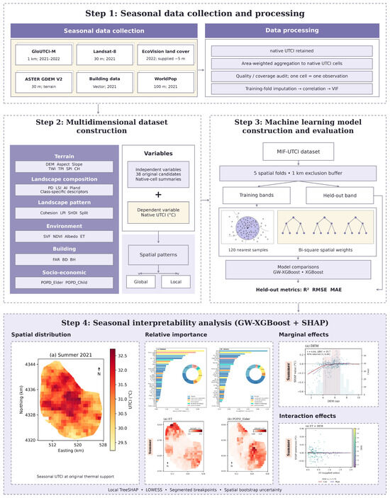
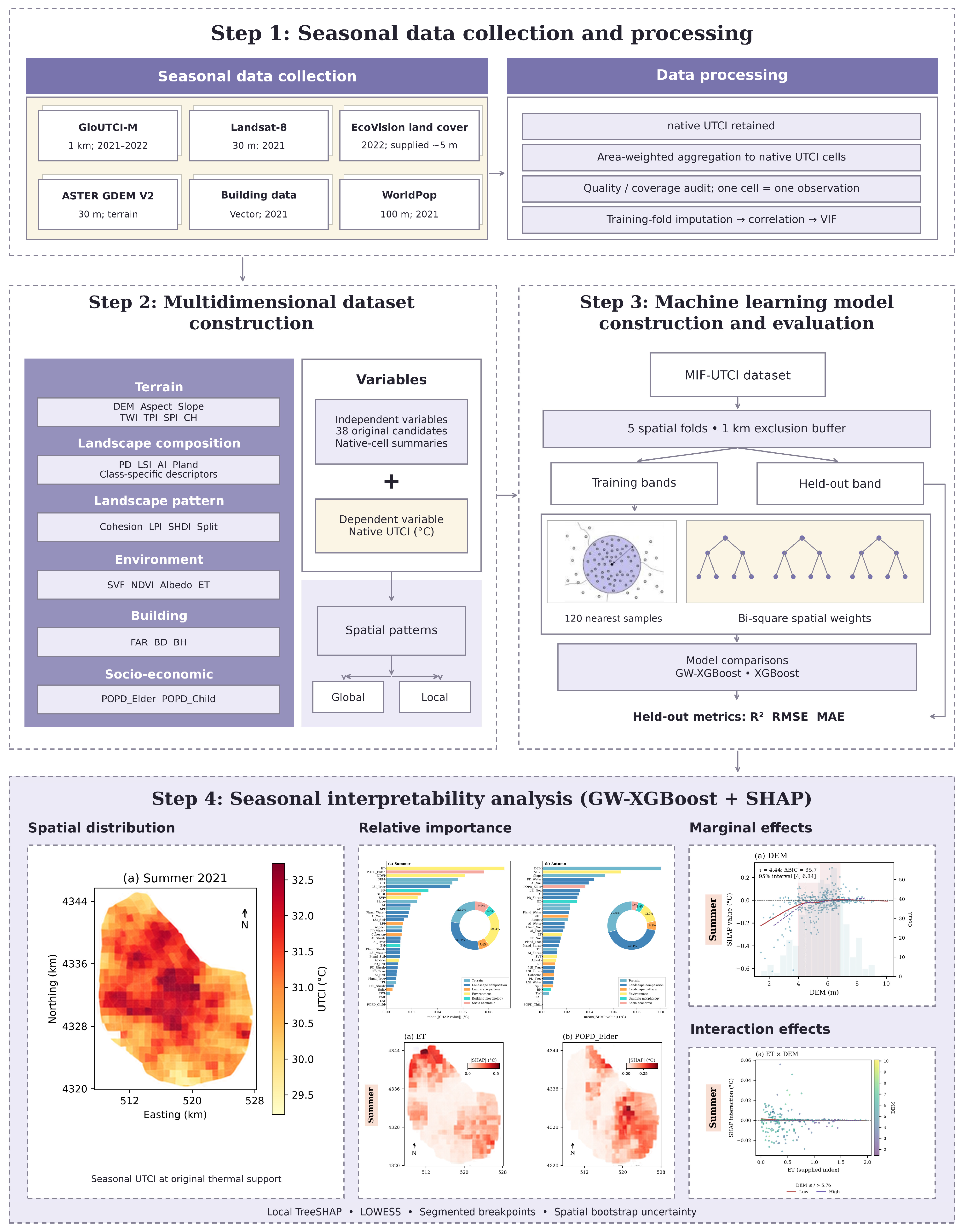
This study established a four-stage technical framework comprising data preparation, indicator construction, model training, and interpretability analysis (Figure 2). Step 1 involved multi-source data acquisition and preprocessing. Step 2 established a multi-dimensional indicator system covering terrain, landscape, and socio-economic elements. Step 3 focused on constructing the GW-XGBoost model using geographically separated validation and comparing its predictive performance with the global XGBoost baseline. Step 4 introduced the SHAP framework to analyze feature contributions and relationships from multiple dimensions, including spatial distribution, nonlinear responses, and conditional interaction patterns. All computational analyses were performed in Python 3.12 using pandas 3.0.5, Rasterio 1.5.1, scikit-learn 1.9.1, XGBoost 3.4.1, and SHAP 0.52.0.
Figure 2.
Research framework. The sub-figures shown in Step 4 are merely illustrative examples of the analytical outputs, which are fully detailed in subsequent result sections (Figures 3–7).
2.4.1. Regression Model
Although tree-ensemble algorithms like XGBoost are inherently resilient to multicollinearity, feature screening was conducted within each training fold to reduce redundant predictors and improve the stability and interpretability of SHAP attribution. The geographically weighted component supplies distance-based weights to local tree ensembles; it is not a separately estimated linear GWR model. Feature screening and imputation were performed independently within each training fold following the procedures described in Section 2.2, without using held-out outcomes or predictor statistics. The full 38-candidate list and retained variables for each season and fold are provided in Table A1.
Model performance was assessed using five-fold geographically separated validation [41]. Native-cell centroids were divided into five contiguous easting-quantile bands. Each band was held out in turn, and training centroids within 1000 m of any test centroid were excluded. Consequently, no subdivision of a native thermal pixel can enter another fold. Training sample counts after buffering ranged from 296 to 323, and test counts from 83 to 85. Coordinates in UTM zone 50N were used for distances.
To capture the spatial non-stationarity of the urban thermal environment, this study constructed a Geographically Weighted Extreme Gradient Boosting (GW-XGBoost) model. The model combines geographically weighted local modeling with the capacity of XGBoost to represent high-dimensional nonlinear relationships [34]. Specifically, GW-XGBoost captures spatial non-stationarity by introducing a geographic weight based on a spatial kernel function into the loss function. For a local model at spatial location , its optimized objective function can be expressed as
In this equation, is the spatial weight from observation point to regression point (calculated in this study using a bi-square kernel with an adaptive bandwidth of 120 nearest training samples); is a differentiable convex loss function; and is the regularization term controlling model complexity.
For each held-out location, the 120 nearest eligible training samples define h, the distance to the 120th neighbor; weights are w = [1 − (d/h)2]2 within h and zero outside. Thus, 120 is a sample count, not meters; 80 and 160 samples provide bandwidth sensitivity checks. XGBoost uses 120 trees, maximum depth 2, learning rate 0.05, minimum child weight 3, L2 regularization 5, and full row/column sampling; the random-forest comparator uses 200 trees and minimum leaf size 3. These hyperparameters were fixed a priori for all validation folds and were not tuned using held-out predictions. All responses and reported SHAP values remain in °C, with random seed 20260913.
To evaluate spatial predictive performance, the GW-XGBoost model was evaluated against the global Extreme Gradient Boosting (XGBoost) baseline using the same held-out native pixels. Comparative metrics including R2, RMSE, and MAE were calculated to assess spatial predictive performance. Performance values are reported in Section 3.1, rather than in the Methods.
2.4.2. Model Interpretation
To interpret the machine-learning model and characterize nonlinear relationships among key factors, this study constructed a joint analytical approach integrating GW-XGBoost, SHAP, and Locally Weighted Scatterplot Smoothing (LOWESS). This methodology enables analysis across three dimensions: global importance, nonlinear response characteristics, and local spatial patterns. First, at the global level, SHAP importance plots were utilized to display the ranking of feature importance, quantifying the relative contribution magnitude of the candidate factors to UTCI predictions. Regarding nonlinear responses and candidate breakpoint identification, we analyzed the relationships between key urban planning factors (e.g., SVF and PD_Water) and UTCI by plotting SHAP Dependence Plots [37]. On this basis, Locally Weighted Scatterplot Smoothing (LOWESS) was introduced to fit the trend of SHAP value scatterplots, with a separate segmented-regression procedure used to quantify candidate breakpoints and uncertainty, and SHAP interaction analysis used to characterize conditional interaction patterns between selected factor pairs. Furthermore, local SHAP values were mapped back to geographic space to characterize the spatial heterogeneity of local feature contributions [39]. Together, these analyses support spatially differentiated interpretation of the modeled UTCI relationships and their potential planning relevance.
Each test sample retains its native_id, centroid coordinates, and original native-pixel polygon. Exact path-dependent TreeSHAP is calculated from that sample’s own geographically weighted model, then joined one-to-one by native_id to map the attribution on the original pixel polygon. The sum of feature contributions plus that local model’s expected value was checked against its prediction (maximum tolerance 10−4 °C). Local expected values differ across locations, and fold-excluded features have zero contribution. The SHAP interaction matrix was checked to sum to the same contributions. The spatial distribution maps display absolute contributions for local importance; The dependence analyses utilize signed contributions. The interaction analysis reports a single off-diagonal matrix entry per pair (not twice that value), together with LOWESS curves for partner values below and above the median.
Quantitative breakpoint identification uses a continuous one-break segmented model: SHAP(x) = β0 + β1x + β2 max(0, x − τ), following the segmented-regression principle. We search 31 quantiles from the 20th to 80th percentile and choose τ minimizing residual sum of squares, requiring at least 15 observations and 10% of the sample on each side. ΔBIC = BIC(linear) − BIC(segmented) = n log(RSSlinear/RSSsegmented) − 2 log(n), counting four parameters for the segmented fit, including τ, versus two for the line. Positive ΔBIC favors the segmented model, whereas negative ΔBIC favors the linear model. ΔBIC is used here for model comparison and should not be interpreted as a formal significance test. Two hundred bootstrap replicates resample occupied 4 km × 4 km spatial tiles with replacement and give 95% percentile intervals. Fold-specific fits and equivalent global XGBoost/random-forest SHAP fits assess stability. The bootstrap intervals are conditional on the fitted SHAP attribution values and do not represent full model-refitting uncertainty. LOWESS was used only for visualization, while breakpoint estimation was based on segmented regression.
3. Results
3.1. Seasonal and Spatial Heterogeneity Patterns of UTCI
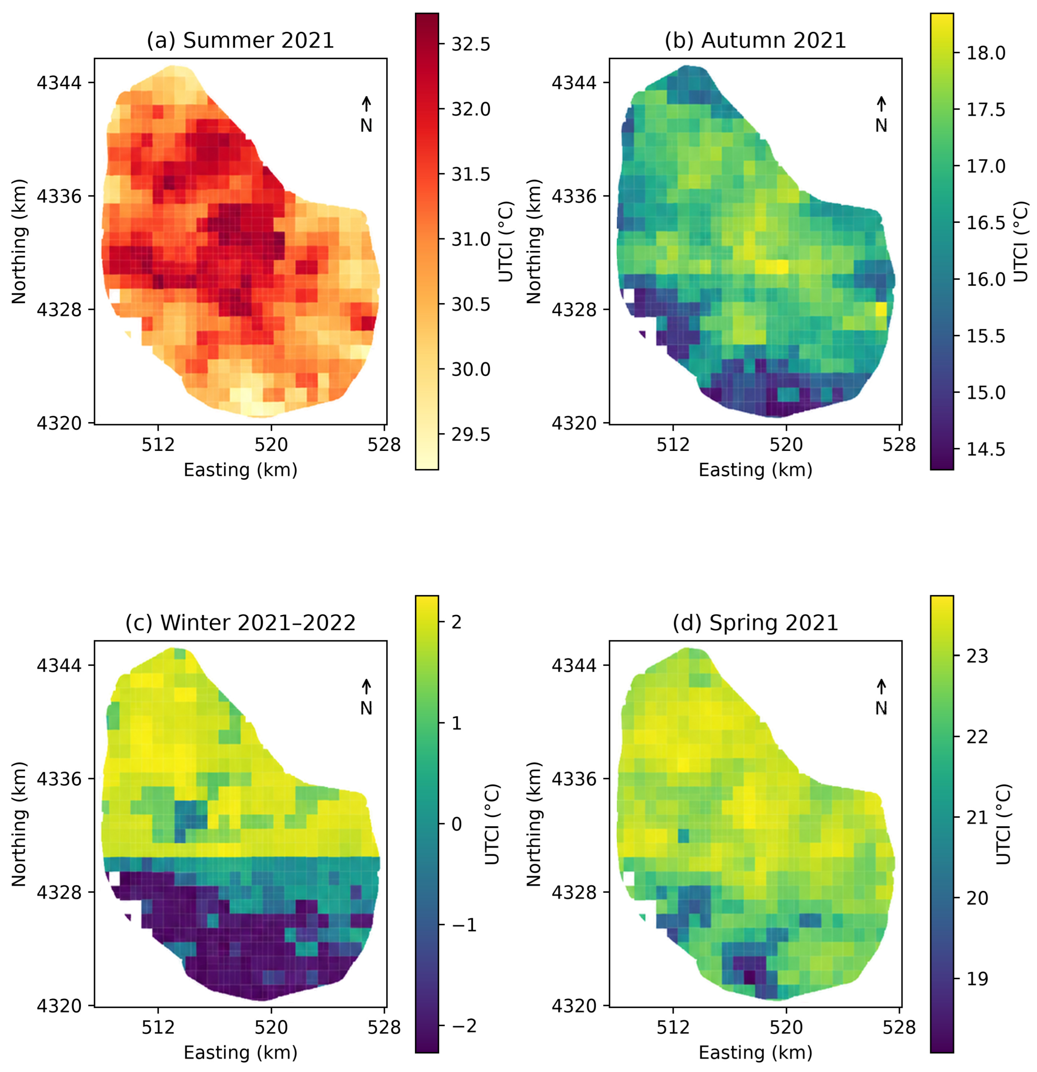
Prior to analyzing the seasonal spatial patterns, model performance was validated on geographically separated test sets. The results demonstrate that the GW-XGBoost model achieved higher mean spatial predictive accuracy across the four seasons (average R2 = 0.408, RMSE = 0.745 °C, MAE = 0.547 °C) compared to the global XGBoost baseline (average R2 = 0.276, RMSE = 0.888 °C, MAE = 0.698 °C). Following this validation, Figure 3 illustrates the seasonal spatial distribution of UTCI within the study area. Spatially, the region exhibits a generally warmer core relative to parts of the periphery across seasons. The magnitude and extent of this spatial gradient differ across seasons.
In terms of spatial distribution, relatively high UTCI values are concentrated in parts of the central and northern-central built-up area, while lower values occur mainly toward the southern and peripheral areas. In summer (Figure 3a), relatively high UTCI values are concentrated in parts of the central built-up area, with a maximum of 32.73 °C. The minimum among the eligible native cells is 29.22 °C, indicating clear spatial variation in summer UTCI. In winter (Figure 3c), a pronounced north–south spatial contrast is observed. Relatively high UTCI values occur across much of the central and northern area, reaching a maximum of 2.26 °C, whereas the southern fringe contains the lowest values, with a minimum of −2.19 °C.
Across seasons, UTCI exhibits marked differences in spatial gradients. In autumn (Figure 3b), relatively high UTCI values occur in parts of the central and northern area, with a maximum of 18.35 °C, whereas lower values occur toward the southern fringe, with a minimum of 14.52 °C. In spring (Figure 3d), relatively high UTCI values occur in parts of the central and northern area, reaching a maximum of 23.71 °C, while lower values occur mainly toward the southern fringe, with a minimum of 18.08 °C. Overall, relatively high UTCI values are repeatedly observed in the central and northern-central portions of the study area, while the magnitude and spatial extent of the contrast with the southern and peripheral areas vary among seasons.
Figure 3.
Seasonal spatial distribution of UTCI across eligible native cells within the study area. (a) Summer; (b) autumn; (c) winter; (d) spring.
3.2. Relative Contributions and Seasonal Shifts in UTCI Driving Factors
Having revealed the seasonal and spatial differentiation of UTCI, this study utilized the GW-XGBoost model to further quantify the relative contributions of the selected predictors to UTCI. The model demonstrated season-dependent spatial predictive performance across the four seasons, with the highest spatial predictive R2 in winter (R2 = 0.678), followed by spring (R2 = 0.411) and autumn (R2 = 0.300), and lower performance in summer (R2 = 0.244). These results indicate clear seasonal differences in the spatial predictive performance of the model.
SHAP-based feature importance (Figure 4) reveals substantial seasonal variation in the relative contributions of predictor categories. The relative contribution of landscape composition increases from summer to winter. In summer (Figure 4a) and autumn (Figure 4b), terrain accounts for 22.5% and 29.4% of the total contribution, respectively, while landscape composition accounts for 30.1% and 42.4%. These results indicate substantial relative contributions from both terrain and landscape composition during summer and autumn. In winter (Figure 4c), the relative contribution of landscape composition increases to 52.7%, exceeding that of terrain (18.1%) and representing the largest category contribution. This indicates a greater relative contribution of landscape composition to the modeled spatial variation in winter UTCI. In spring (Figure 4d), landscape composition remains the largest category (42.4%), followed by terrain (27.8%).
At the individual-feature level, the rankings also vary across seasons. In summer, ET and Elderly Population Density (POPD_Elder) rank first and second, followed by NDVI and elevation (DEM). The Socioeconomic category reaches its highest contribution among the four seasons at 9.9% in summer, indicating a relatively stronger modeled contribution of population-related variables during this season. Autumn is led by DEM and NDVI, followed by Slope. In spring (Figure 4d), ET ranks first, followed by Pland_Water and Slope, indicating notable contributions from environmental, landscape composition, and terrain variables. In winter, the top five features are Building Density (BD), AI, Pland_Water, the Bare Land Landscape Shape Index (LSI_Soil), and Water Aggregation (AI_Water), indicating relatively large contributions from building-morphology and landscape composition variables.
In summary, the relative contributions of UTCI predictors vary substantially across seasons, with landscape composition contributing more strongly in winter than in summer. Terrain, environmental, socioeconomic, building-morphology, and landscape variables also show season-dependent changes in their relative importance, indicating a clear seasonal reorganization of the modeled feature contributions.
Figure 5 illustrates the spatial distribution of local feature importance, revealing substantial spatial heterogeneity in the contributions of individual predictors to UTCI. Unlike the global feature-importance rankings, the local SHAP maps identify areas of relatively high predictor importance by quantifying feature contributions at each native UTCI cell. The maps therefore represent local importance intensity at the native UTCI-cell support. Figure 5 presents the three leading factors for each season using absolute SHAP magnitudes, while the directions of their contributions are examined using signed SHAP values in the dependence plots.
Socioeconomic, environmental, and terrain variables exhibit distinct spatial patterns of local importance across seasons. In summer, high absolute SHAP magnitudes for Elderly Population Density (POPD_Elder; Figure 5b) are concentrated in parts of the central and eastern built-up area, with a peak local contribution of 0.459 °C. ET (Figure 5a) shows relatively high local importance in the northern part of the study area, whereas NDVI (Figure 5c) exhibits a more concentrated central pattern. In autumn, terrain variables show pronounced spatial variation in local importance. High absolute SHAP magnitudes for Elevation (DEM; Figure 5d) are concentrated toward the southern and southwestern fringe, reaching a peak contribution of 1.097 °C, while Slope (Figure 5f) also exhibits elevated local importance along parts of the western and southern fringe. These patterns demonstrate distinct spatial footprints of predictor importance across seasons.
Figure 4.
Global feature-importance ranking of explanatory factors based on mean absolute SHAP values across four seasons. (a) Summer; (b) autumn; (c) winter; (d) spring.
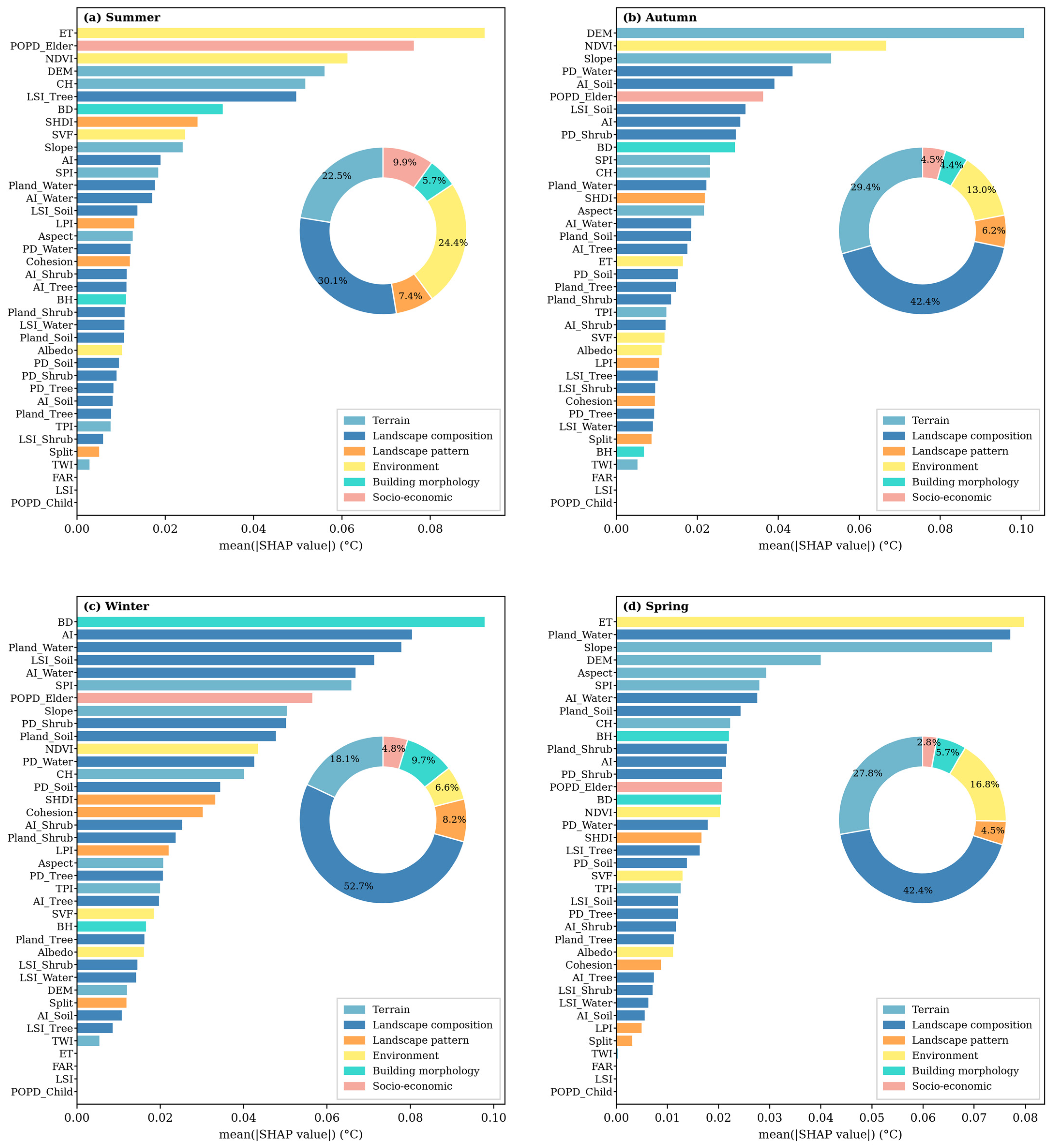
Figure 5.
Spatial distribution of local feature importance for the three leading drivers in each season. (a) ET; (b) POPD_Elder; (c) NDVI; (d) DEM; (e) NDVI; (f) Slope; (g) BD; (h) AI; (i) Pland_Water; (j) ET; (k) Pland_Water; (l) Slope.
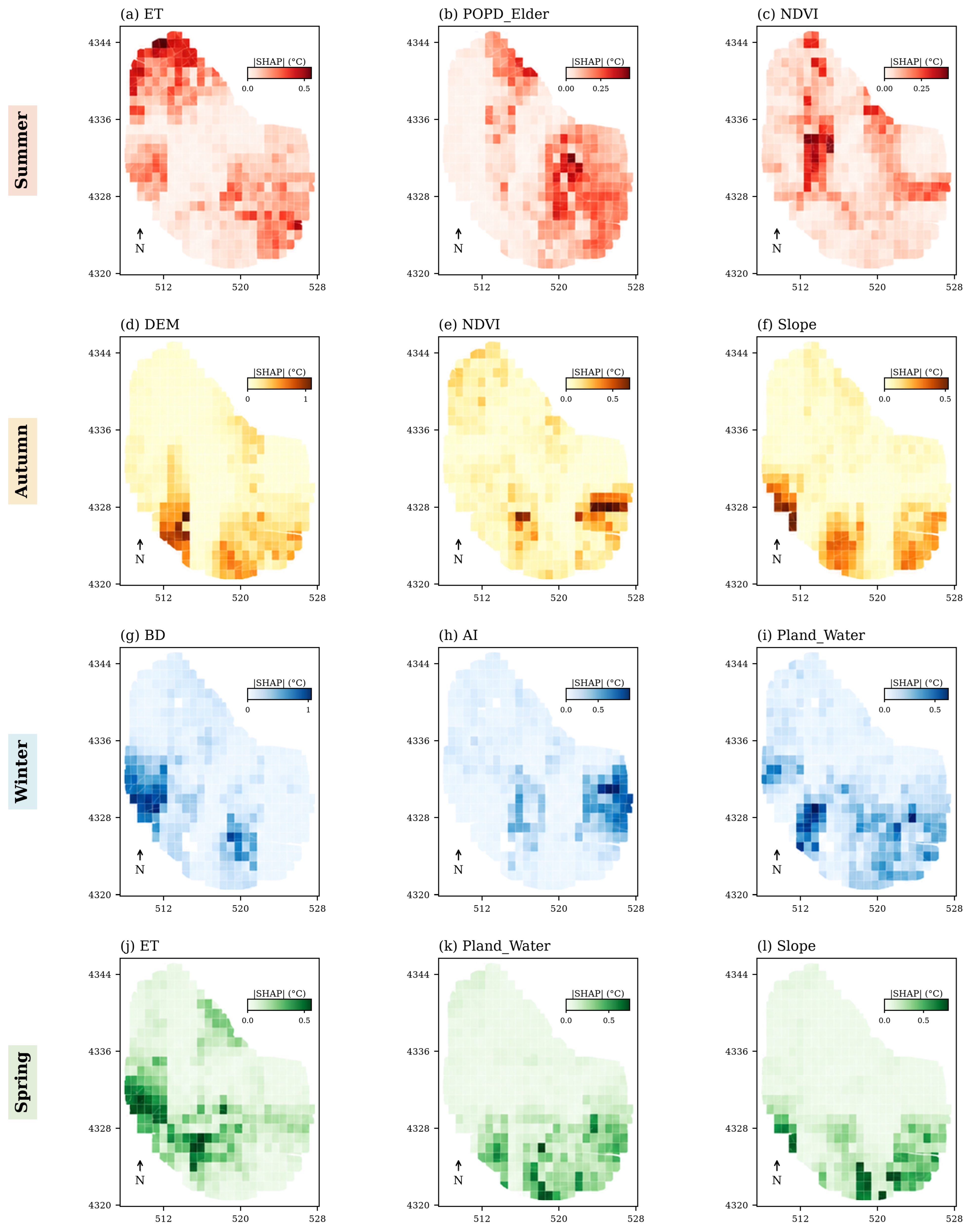
Landscape composition and building-morphology variables also exhibit spatially heterogeneous importance patterns. Water cover (Pland_Water; Figure 5i,k) shows relatively high absolute SHAP magnitudes in western portions of the study area in winter and a more southerly concentration in spring, with peak contributions of 0.631 °C and 0.744 °C, respectively. This indicates season-dependent spatial variation in the local importance of water-related landscape composition. In winter, high absolute SHAP magnitudes for Building Density (BD; Figure 5g) are concentrated in the western part of the study area, reaching a maximum of 1.050 °C, whereas AI, a landscape composition metric, exhibits relatively high local importance in the eastern area (Figure 5h). These contrasting spatial patterns further demonstrate the seasonal and spatial heterogeneity of local predictor importance.
3.3. SHAP Dependence Relationships and Candidate Breakpoints of Key Driving Factors
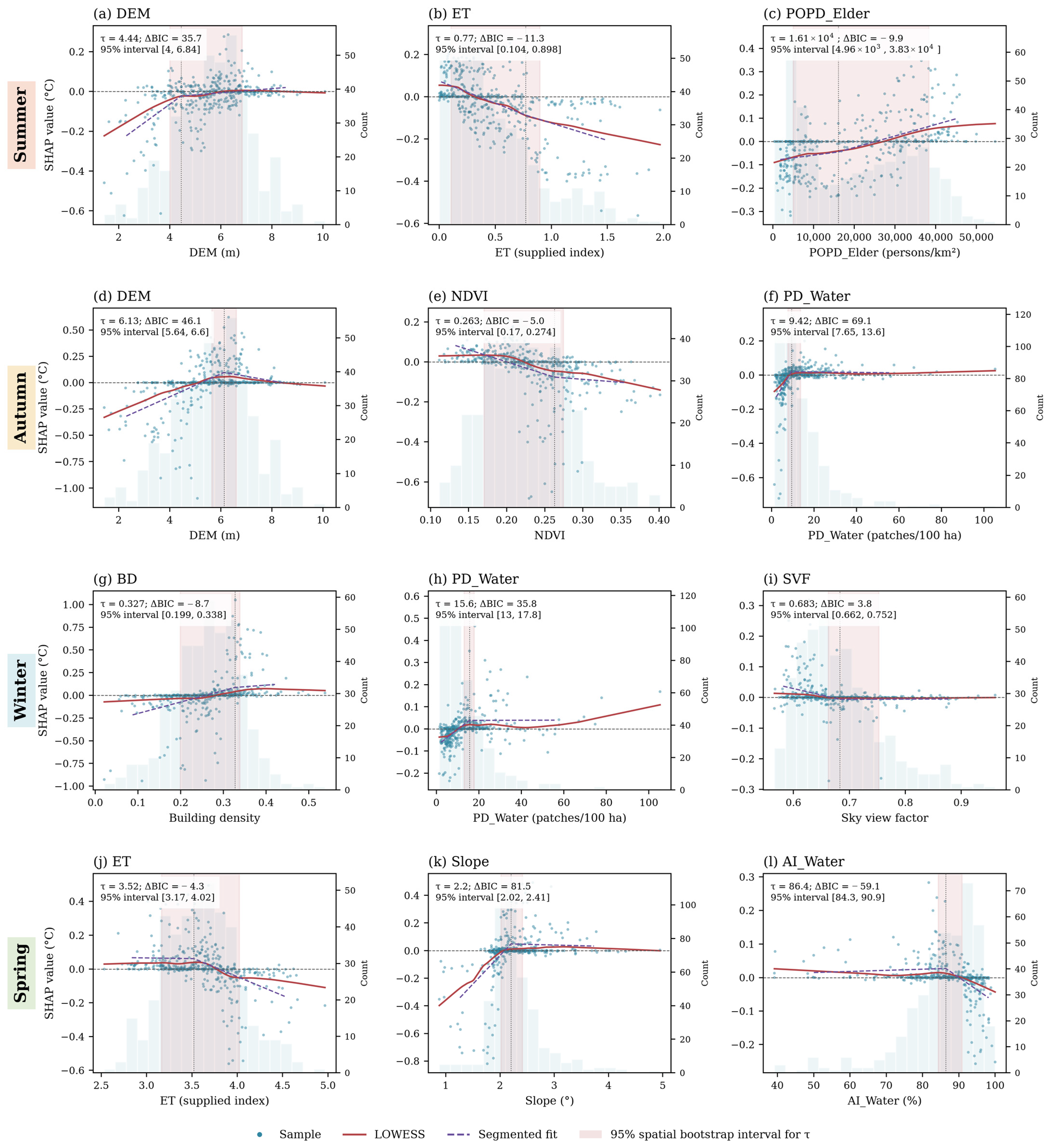
Following the spatial analysis of predictor importance, Figure 6 further examines the functional form of SHAP relationships between key predictors and UTCI, including both approximately linear and nonlinear patterns. Figure 6 presents signed SHAP dependence relationships together with LOWESS trends and segmented fits, allowing comparison between approximately linear responses and candidate nonlinear breakpoints. Each seasonal row displays three factors, together with quantitative segmented-fit estimates, ΔBIC values, and 95% spatial-bootstrap intervals. Positive ΔBIC favors the segmented description, whereas negative ΔBIC favors the linear description.
Socioeconomic variables show a gradual rather than sharply bounded relationship in summer. Elderly Population Density (POPD_Elder; Figure 6c) exhibits a generally increasing relationship with SHAP values, while the model comparison favors a linear description (ΔBIC = −9.9), indicating a gradual density-related association rather than a well-supported breakpoint. Terrain variables show clearer evidence of nonlinear responses. For DEM, the estimated breakpoints are 4.44 m in summer (Figure 6a) and 6.13 m in autumn (Figure 6d), with 95% spatial-bootstrap intervals of 4–6.84 m and 5.64–6.6 m, respectively. The corresponding ΔBIC values are 35.7 and 46.1, supporting segmented descriptions. Below these estimates, fitted SHAP values generally increase with elevation; beyond them, the summer curve flattens while the autumn segmented curve turns downward.
Environmental predictors exhibit different functional forms across seasons. In summer, SHAP values for ET (Figure 6b) generally decline as the supplied ET index increases, while the model comparison favors a linear description (ΔBIC = −11.3). Similarly, autumn NDVI (Figure 6e) shows a generally negative association, with the linear description favored over the one-break model (ΔBIC = −5.0). In contrast, Water Patch Density (PD_Water; Figure 6f) in autumn shows an increasing response followed by flattening, with an estimated breakpoint of 9.42 patches/100 ha (95% interval 7.65–13.6; ΔBIC = 69.1). These results demonstrate that response shape and statistical support for a specific breakpoint should be distinguished.
In winter and spring, building-morphology and water-related predictors also exhibit contrasting functional forms. The winter Sky View Factor (SVF; Figure 6i) declines toward zero before flattening near 0.683 (95% interval 0.662–0.752; ΔBIC = 3.8), providing modest support for a change in slope. Winter PD_Water (Figure 6h) shows stronger segmented support, increasing below approximately 15.6 patches/100 ha and becoming nearly flat above this level (95% interval 13–17.8; ΔBIC = 35.8). In contrast, Building Density (Figure 6g) is better described by a linear relationship (ΔBIC = −8.7). In spring, AI_Water (Figure 6l) shows a downturn near 86.4% (95% interval 84.3–90.9; ΔBIC = 59.1), while ET (Figure 6j) and Slope (Figure 6k) show estimated changes near 3.52 and 2.2°, respectively. Where ΔBIC is positive, these segmented-fit estimates are interpreted as candidate statistical breakpoints and locally testable nonlinear reference points rather than fixed planning thresholds. Where ΔBIC is negative, the linear description is preferred, and the segmented-fit estimate is not interpreted as a supported breakpoint.
Figure 6.
(a–l) SHAP dependence relationships and candidate breakpoints for selected driving factors across four seasons. (a) DEM; (b) ET; (c) POPD_Elder; (d) DEM; (e) NDVI; (f) PD_Water; (g) BD; (h) PD_Water; (i) SVF; (j) ET; (k) Slope; (l) AI_Water. The red solid lines represent the Locally Weighted Scatterplot Smoothing (LOWESS) trends, and the purple dashed lines indicate the segmented-regression fits.
3.4. Conditional Interaction Patterns Among Key Driving Factors
Figure 7 further characterizes conditional interaction patterns between selected pairs of key predictors across seasons. In summer, the ET–DEM interaction (Figure 7a) has a mean absolute interaction contribution of 0.0032 °C. The fitted curves for lower and higher DEM groups remain close to zero over much of the ET range, although individual observations exhibit both positive and negative interaction contributions. The ET–POPD_Elder interaction (Figure 7b) shows clearer differentiation between Population Density contexts mainly at lower ET values, with the fitted curves converging as ET increases. The ET–CH interaction (Figure 7c) likewise shows variation in the ET interaction pattern across canopy-height contexts.
Figure 7.
(a–l) SHAP interaction dependence plots for selected driver pairs across four seasons. (a) ET × DEM; (b) ET × POPD_Elder; (c) ET × CH; (d) DEM × PD_Water; (e) DEM × AI_Soil; (f) NDVI × PD_Water; (g) AI × LPI; (h) BD × Pland_Water; (i) AI × PD_Water; (j) DEM × Pland_Water; (k) ET × SPI; (l) Slope × Pland_Water.
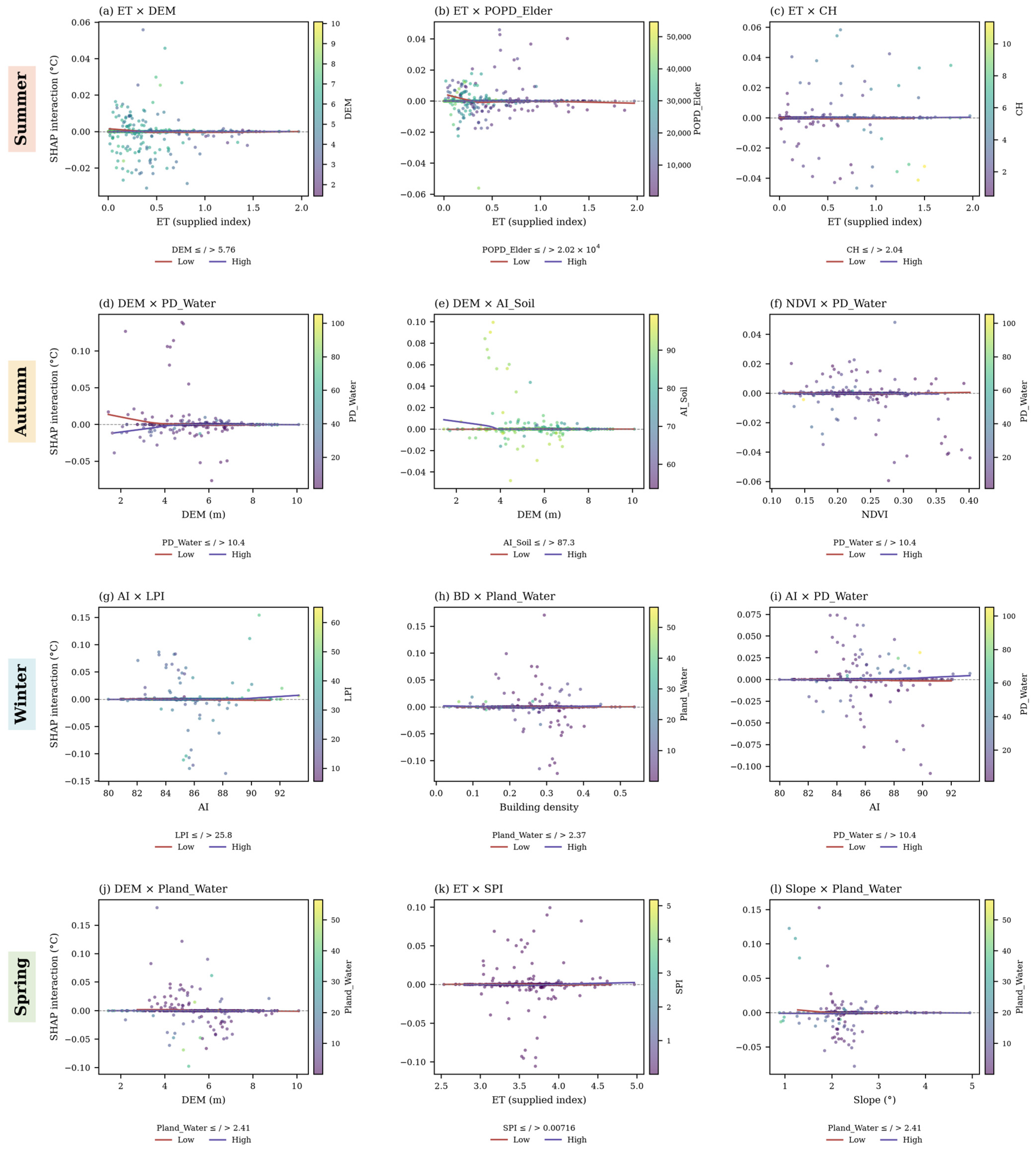
Autumn and spring exhibit different combinations of terrain, vegetation, and water-related interactions. In autumn, the DEM–PD_Water interaction (Figure 7d) has a mean absolute interaction contribution of 0.0043 °C. At lower elevations, the fitted curve for the lower PD_Water group is more positive than that for the higher PD_Water group, while both approach zero as elevation increases. The DEM–AI_Soil and NDVI–PD_Water pairs (Figure 7e,f) show additional conditional differences. In spring (Figure 7j–l), the selected interactions involve DEM–Pland_Water, ET–SPI, and Slope–Pland_Water. Among these, DEM–Pland_Water has the largest mean absolute interaction contribution at 0.0057 °C. These seasonal differences indicate changes in the combinations of predictors exhibiting the strongest interaction contributions.
Winter interactions are concentrated among landscape composition, landscape pattern, and building-morphology variables. The AI–Largest Patch Index (LPI) interaction (Figure 7g) has the largest mean absolute interaction contribution at 0.0060 °C. Although individual observations show both positive and negative interaction contributions, the fitted curves remain close to zero across much of the AI range. The Building Density–water cover (BD–Pland_Water) interaction (Figure 7h) has a mean absolute contribution of 0.0057 °C, followed by AI–PD_Water at 0.0052 °C (Figure 7i). Overall, the winter results indicate that building morphology and landscape characteristics exhibit stronger conditional interaction contributions than those observed for the selected summer pairs.
4. Discussion
4.1. Seasonal Heterogeneity of Urban Thermal-Environment Regulation Mechanisms
This study indicates that the associations between UTCI and its predictors vary substantially across seasons [43,44,45]. Such seasonal variation suggests that thermal-comfort priorities differ between hot and cold periods: summer interventions primarily focus on limiting heat stress, whereas winter strategies need to consider the maintenance of outdoor thermal comfort under cold conditions.
Urban-form and radiative-exposure conditions also show season-dependent associations with UTCI. In summer, lower SVF may increase shading and reduce direct solar exposure, thereby contributing to lower daytime thermal loads [46,47]. In winter, the SVF relationship shows a candidate breakpoint near 0.683 (Figure 6i). Below this estimate, the fitted SHAP contribution declines as SVF increases, whereas above it the fitted relationship remains close to zero. A possible physical interpretation, consistent with previous studies, is that more enclosed urban spaces can provide shelter from cold airflow and reduce convective heat exchange [45]. Given the modest ΔBIC support and bootstrap uncertainty, 0.683 should therefore be interpreted as a candidate morphological reference for local testing rather than as a fixed physical or design boundary.
During cooler periods, differences in local surface orientation and exposure may also influence thermal comfort through variations in received solar radiation. In highly urbanized areas, these surface orientation effects may coexist with the influence of built morphology on shading and airflow. These processes provide a possible physical context for the observed statistical associations.
Water-related landscape variables likewise exhibit season-dependent relationships with UTCI. In summer, previous studies have shown that water bodies can reduce surrounding thermal loads through evaporative cooling [22,48]. In winter, the SHAP dependence relationship for Water Patch Density (PD_Water; Figure 6h) increases below approximately 15.6 patches/100 ha and becomes nearly flat above this level. This pattern is consistent with the potential role of water-related landscapes as local microclimate stabilizers under cold conditions [49,50]. One possible interpretation is that water heat-storage processes may contribute to relatively moderated thermal conditions in surrounding areas. These findings suggest potential value in maintaining functional blue-green networks, while their specific thermal performance should be evaluated under local conditions.
4.2. Nonlinear Breakpoints and Conditional Interactions Among Driving Factors
Beyond seasonal variation in predictor importance, the results identify candidate nonlinear breakpoints for several UTCI relationships [51,52] together with conditional interaction patterns among selected predictors. Their planning interpretation should therefore consider both estimated numerical ranges and their associated uncertainty.
Socioeconomic variables exhibit comparatively gradual associations with UTCI. In summer, Elderly Population Density (Figure 6c) shows a generally increasing SHAP relationship, while model comparison favors a linear description rather than a segmented breakpoint. Population distribution therefore remains relevant to thermal exposure and vulnerability [53,54]. In contrast, several environmental and landscape variables show stronger support for candidate nonlinear relationships [55]. Winter PD_Water exhibits a change in slope near 15.6 patches/100 ha (Figure 6h), whereas SVF shows a weaker candidate change near 0.683 (Figure 6i) [56,57]. The corresponding spatial-bootstrap intervals quantify the uncertainty around these estimates and support their interpretation as locally testable statistical reference points rather than exact planning standards.
Conditional interaction patterns also vary across seasons [58,59]. In summer, the ET–DEM interaction (Figure 7a) remains close to zero across much of the ET range, while the ET–population interaction (Figure 7b) shows greater differentiation between population contexts at lower ET values. In autumn, DEM–PD_Water (Figure 7d) exhibits conditional differences at lower elevations, whereas spring interactions involve combinations of water cover, terrain, and environmental variables (Figure 7j–l). In winter, the selected interactions are concentrated among building-morphology and landscape variables, with AI–LPI and BD–Pland_Water showing relatively large mean absolute interaction contributions (Figure 7g,h). These seasonal differences highlight the importance of considering predictor combinations and their conditional relationships rather than interpreting individual factors in isolation.
4.3. Spatial Planning Strategies for Climate-Adaptive Cities
The results suggest that urban thermal-environment planning should account for seasonally varying spatial associations, candidate nonlinear breakpoints, and local validation rather than relying on uniform interventions [60,61,62]. Planning responses should also distinguish between existing urban regeneration areas and new development areas because their capacities for modifying urban form differ substantially.
For existing urban regeneration areas, where large-scale modification of buildings, roads, and property boundaries is often constrained, thermal adaptation may prioritize incremental and surface-oriented interventions. Population Density shows a gradual association with summer thermal conditions (Figure 6c), making thermal exposure and local microclimate conditions relevant considerations for regeneration planning. In high-density built-up areas, interventions can therefore emphasize quality-oriented improvements, including vertical greening, high-reflectance coatings, permeable surface treatments, and enhancement of existing blue-green connections [63,64], rather than relying primarily on large-scale reductions in development intensity.
For new development areas and urban fringes, greater spatial flexibility allows climate adaptation to be incorporated before urban form and development intensity are fixed. Ventilation corridors may be reserved where local wind and thermal assessments support their effectiveness [65], while street-canyon geometry, solar exposure, and blue-green infrastructure can be coordinated during the initial planning stage. The winter SVF breakpoint near 0.683 (Figure 6i; 95% interval 0.662–0.752) may serve as a candidate quantitative reference for local testing of street-canyon conditions rather than as a mandatory design limit. Compact urban forms may enhance winter shelter while also constraining summer ventilation [66,67]; consequently, open-space and street-canyon design should jointly consider solar exposure, wind conditions, and seasonal thermal objectives [68].
Landscape planning should likewise consider landscape composition and configuration rather than coverage alone. The winter PD_Water estimate near 15.6 patches/100 ha (Figure 6h) represents an area-weighted patch-density descriptor rather than a water-cover percentage. Water cover, aggregation, patch density, and surrounding morphology can therefore be assessed jointly when evaluating cold-season thermal conditions [69,70]. In naturally moisture-retaining areas and existing drainage or blue-green corridors, planning may prioritize the preservation of permeable and vegetated surfaces and avoid unnecessary sealing or concreting. Vegetation placement can additionally account for terrain, moisture availability, and existing blue-green networks [71,72], supporting evapotranspirative cooling while allowing possible cold-season buffering effects to be evaluated locally.
4.4. Limitations
Although this study has advanced the quantitative understanding of season-dependent associations and candidate nonlinear breakpoints of urban thermal comfort (UTCI), several limitations remain. Constrained by the spatiotemporal resolution of multi-source data, uncertainties persist in characterizing the heterogeneity of micro-scale thermal environments. In addition, although explanatory variables were aggregated to the native UTCI grid, residual uncertainty associated with the Modifiable Areal Unit Problem (MAUP) remains. While candidate nonlinear breakpoints were estimated, current raster data struggle to precisely capture the refined impact of instantaneous wind fields and complex shadows within street canyons on human thermal experience, particularly regarding radiant heat load. Some explanatory variables focus on passive physical regulation, while active anthropogenic heat sources such as traffic and air-conditioning exhaust are not directly represented, which limits model explanatory power in high-intensity activity zones. Furthermore, although SHAP interaction analysis identifies nonlinear associations, it is fundamentally based on statistical correlation. It currently lacks physical validation of fluid-dynamic processes within ventilation corridors and requires further process-based validation of energy-transfer mechanisms. Future work could expand on multi-source data fusion and mechanism coupling, incorporating airborne LiDAR to build sub-meter 3D urban canopy models to enhance data precision, and combining crowd movement data to explore the transition from static evaluation to dynamic thermal comfort assessment. The analysis covers a single seasonal cycle and integrates multi-source datasets with differing spatial and temporal resolutions. In addition, the reported bootstrap intervals are conditional on the fitted SHAP attribution values. Future studies incorporating multi-year observations and higher-resolution data could further evaluate the robustness and transferability of the identified seasonal relationships.
5. Conclusions
This study developed an interpretable spatial machine learning framework integrating GW-XGBoost and SHAP to investigate the seasonal differentiation of urban thermal comfort in the central urban area of Tianjin, China. By jointly considering nonlinear responses and spatial non-stationarity, the study systematically revealed the seasonal and spatial differentiation of UTCI across its native grid and the season-dependent associations of its explanatory factors. The findings provide quantitative evidence for climate-adaptive thermal-environment management and sustainable urban planning. The main conclusions are as follows.
First, UTCI exhibits pronounced spatial structure and seasonal differences in thermal gradients. Across all four seasons, the study area generally maintains higher UTCI values in the core relative to parts of the periphery. In summer, relatively high UTCI values are concentrated in parts of the central built-up area, reaching a maximum of 32.73 °C. In winter, relatively high UTCI values occur across much of the central and northern area, reaching a maximum of 2.26 °C, whereas the minimum among eligible native cells is −2.19 °C. Across seasons, autumn values range from 14.52 °C to 18.35 °C and spring values from 18.08 °C to 23.71 °C, demonstrating pronounced seasonal differences in spatial thermal gradients. These findings indicate substantial seasonal variation in the spatial distribution of urban thermal comfort, which should therefore be considered in season-specific climate adaptation.
Second, the relative contributions of UTCI predictors exhibit substantial seasonal shifts. In summer and autumn, environmental, terrain, and socioeconomic variables all contribute to the modeled UTCI variation, with ET leading in summer and DEM in autumn. In winter, the leading individual factor is Building Density and the largest category is landscape composition, indicating increased relative contributions from building-morphology and landscape composition variables. Overall, predictor importance changes markedly across seasons, highlighting the need to move beyond uniform year-round thermal-environment interventions toward seasonally adaptive urban design.
Third, candidate nonlinear breakpoints were quantified for selected predictors using segmented fits and spatial-bootstrap intervals. The gradual association of Elderly Population Density with summer thermal conditions highlights the relevance of complementary surface and microclimate strategies in density-related planning. The SVF breakpoint of approximately 0.683 has a 95% interval of 0.662–0.752. In addition, winter PD_Water exhibits a change in slope near 15.6 patches/100 ha (95% interval 13–17.8), while spring AI_Water turns downward near 86.4% (95% interval 84.3–90.9). These estimates provide candidate quantitative reference points for local testing of street-canyon design and blue-green infrastructure planning rather than fixed planning thresholds.
Fourth, season-dependent conditional interaction patterns were identified among selected predictors. In summer, leading interaction patterns involve ET together with DEM, Population Density, and canopy height. In winter, AI–LPI and Building Density–Water Cover are among the interaction pairs with relatively large mean absolute contributions. These results indicate that thermal-comfort interventions should consider not only individual factors but also conditional predictor combinations and their seasonal context.
In summary, this study advances the understanding of urban thermal comfort from the identification of general predictor importance toward the quantification of season-specific nonlinear relationships and candidate breakpoints, spatially heterogeneous contributions, and conditional interaction patterns. By translating these findings into uncertainty-informed, locally testable, and spatially differentiated planning guidance, the study provides quantitative support for climate-adaptive urban design, including differentiated density management, seasonally responsive urban morphology, and targeted blue-green infrastructure interventions. More broadly, the proposed framework contributes to improving urban thermal resilience and outdoor livability and provides an evidence base for more sustainable urban development under intensifying climate and urbanization pressures.
Author Contributions
Conceptualization, L.L., Y.Y. (Yan Yang) and J.W.; methodology, L.L., Y.Y. (Yan Yang), Y.Y. (Yang Yu) and J.W.; software, L.L., Y.Y. (Yan Yang), Y.Y. (Yang Yu) and Z.W. (Zhenkun Wang); validation, Y.Y. (Yan Yang), H.W., Z.W. (Zhenkun Wang), L.H. and S.Z.; formal analysis, L.L. and Y.Y. (Yan Yang); investigation, H.W., Z.W. (Zixian Wu), L.C., Q.W. and S.Z.; resources, Z.W. (Zixian Wu), Q.W. and J.W.; data curation, L.L. and Z.W. (Zixian Wu); writing—original draft preparation, L.L. and Y.Y. (Yan Yang); writing—review and editing, L.L., Y.Y. (Yan Yang) and J.W.; visualization, L.L., H.W., L.C. and L.H.; supervision, J.W.; project administration, J.W. All authors have read and agreed to the published version of the manuscript.
Funding
This research received no external funding.
Institutional Review Board Statement
Not applicable.
Informed Consent Statement
Not applicable.
Data Availability Statement
The data presented in this study are available on request from the corresponding author.
Conflicts of Interest
The authors declare no conflicts of interest.
Appendix A. Spatial Validation and Sensitivity Analyses
Figure A1.
Five geographically separated validation bands used for spatial cross-validation.
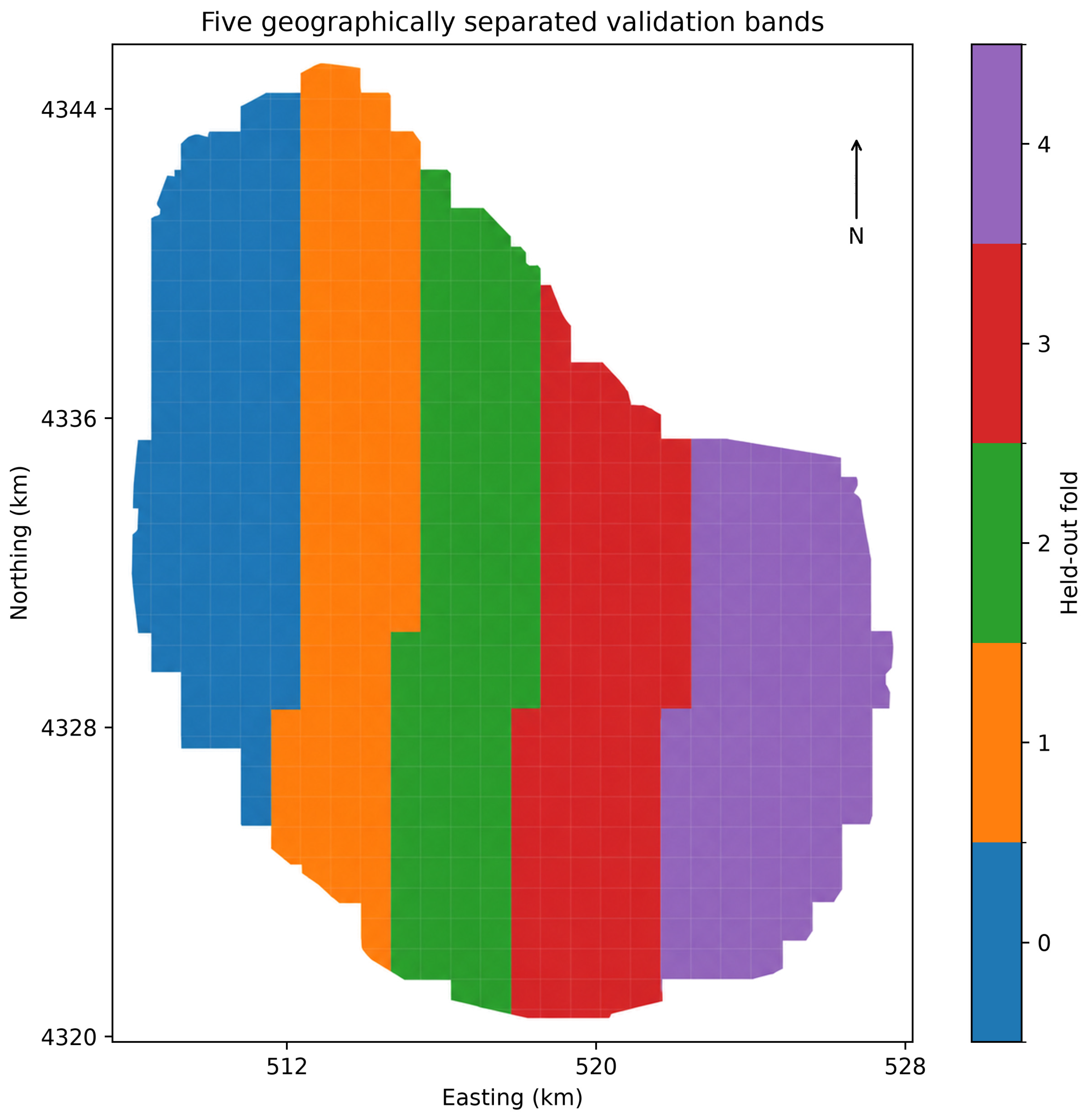
Table A1.
Fold-specific retention of candidate predictors by season (folds 0–4; 1 = retained, 0 = removed).
Table A2.
Candidate breakpoint estimates, model-comparison evidence, and sensitivity results for the displayed Figure 6 panels and additional cases. ΔBIC > 0 favors a segmented description; it is not a significance test. Intervals are conditional on fitted SHAP values. PD uses patches/100 ha, Pland and AI use %, DEM uses m, population uses persons/km2, Aspect/Slope use degrees; other supplied indices are unscaled. Alternative-model break locations are provided only as sensitivity references and should not be interpreted as evidence that a segmented model is preferred in those alternative models.
Table A3.
Local bandwidth and coverage sensitivities. Bandwidth is a sample count; h is the resulting physical radius. Coverage ≥75% uses the same out-of-fold predictions on a subset, not a separately refitted model.
References
- He, X.; Wang, J.; Feng, J.; Yan, Z.; Miao, S.; Zhang, Y.; Xia, J. Observational and modeling study of interactions between urban heat island and heatwave in Beijing. J. Clean. Prod. 2020, 247, 119169. [Google Scholar] [CrossRef] [Scilit]
- Stone, B.; Hess, J.; Frumkin, H. Urban Form and Extreme Heat Events: Are Sprawling Cities More Vulnerable to Climate Change Than Compact Cities? Environ. Health Perspect. 2010, 118, 1425–1428. [Google Scholar] [CrossRef] [Scilit] [PubMed]
- Zhou, D.; Xiao, J.; Frolking, S.; Zhang, L.; Zhou, G. Urbanization Contributes Little to Global Warming but Substantially Intensifies Local and Regional Land Surface Warming. Earth’s Future 2022, 10, e2021EF002401. [Google Scholar] [CrossRef] [Scilit]
- Abd Elraouf, R.; Elmokadem, A.; Megahed, N.; Eleinen, O.; Eltarabily, S. Evaluating urban outdoor thermal comfort: A validation of ENVI-met simulation through field measurement. J. Build. Perform. Simul. 2022, 15, 268–286. [Google Scholar] [CrossRef] [Scilit]
- Afshari, A.; Vogel, J.; Chockalingam, G. Statistical Downscaling of SEVIRI Land Surface Temperature to WRF Near-Surface Air Temperature Using a Deep Learning Model. Remote Sens. 2023, 15, 4447. [Google Scholar] [CrossRef] [Scilit]
- Tran, D.-P.; Liou, Y.-A. Creating a spatially continuous air temperature dataset for Taiwan using thermal remote-sensing data and machine learning algorithms. Ecol. Indic. 2024, 158, 111469. [Google Scholar] [CrossRef] [Scilit]
- Cao, S.; Weng, Q.; Lu, L. Distinctive roles of two- and three-dimensional urban structures in surface urban heat islands over the conterminous United States. Urban Clim. 2022, 44, 101230. [Google Scholar] [CrossRef] [Scilit]
- Du, S.; Wu, Y.; Guo, L.; Fan, D.; Sun, W. How Does the 2D/3D Urban Morphology Affect the Urban Heat Island across Urban Functional Zones? A Case Study of Beijing, China. ISPRS Int. J. Geo-Inf. 2024, 13, 120. [Google Scholar] [CrossRef] [Scilit]
- Blazejczyk, K.; Epstein, Y.; Jendritzky, G.; Staiger, H.; Tinz, B. Comparison of UTCI to selected thermal indices. Int. J. Biometeorol. 2012, 56, 515–535. [Google Scholar] [CrossRef] [Scilit] [PubMed]
- Blazejczyk, K.; Jendritzky, G.; Bröde, P.; Fiala, D.; Havenith, G.; Epstein, Y.; Psikuta, A.; Kampmann, B. An introduction to the Universal Thermal Climate Index (UTCI). Geogr. Pol. 2013, 86, 5–10. [Google Scholar] [CrossRef] [Scilit]
- Fiala, D.; Havenith, G.; Bröde, P.; Kampmann, B.; Jendritzky, G. UTCI-Fiala multi-node model of human heat transfer and temperature regulation. Int. J. Biometeorol. 2011, 56, 429–441. [Google Scholar] [CrossRef] [Scilit] [PubMed]
- Park, S.; Tuller, S.E.; Jo, M. Application of Universal Thermal Climate Index (UTCI) for microclimatic analysis in urban thermal environments. Landsc. Urban Plan. 2014, 125, 146–155. [Google Scholar] [CrossRef] [Scilit]
- Mohammadi, M.; Khoorani, A. Spatiotemproal changes and hot spots of UTCI index over Iran. Urban Clim. 2024, 56, 102031. [Google Scholar] [CrossRef] [Scilit]
- Shi, T.; Yang, Y.; Qi, P.; Lolli, S. Diurnal variation in an amplified canopy urban heat island during heat wave periods in the megacity of Beijing: Roles of mountain–valley breeze and urban morphology. Atmos. Chem. Phys. 2024, 24, 12807–12822. [Google Scholar] [CrossRef] [Scilit]
- Jandaghian, Z.; Colombo, A. The Role of Water Bodies in Climate Regulation: Insights from Recent Studies on Urban Heat Island Mitigation. Buildings 2024, 14, 2945. [Google Scholar] [CrossRef] [Scilit]
- Ren, Z.; Wang, C.; Guo, Y.; Hong, S.; Zhang, P.; Ma, Z.; Hong, W.; Wang, X.; Geng, R.; Meng, F. The cooling capacity of urban vegetation and its driving force under extreme hot weather: A comparative study between dry-hot and humid-hot cities. Build. Environ. 2024, 263, 111901. [Google Scholar] [CrossRef] [Scilit]
- Santamouris, M. Using cool pavements as a mitigation strategy to fight urban heat island—A review of the actual developments. Renew. Sustain. Energy Rev. 2013, 26, 224–240. [Google Scholar] [CrossRef] [Scilit]
- Guo, A.; Yang, J.; Sun, W.; Xiao, X.; Xia Cecilia, J.; Jin, C.; Li, X. Impact of urban morphology and landscape characteristics on spatiotemporal heterogeneity of land surface temperature. Sustain. Cities Soc. 2020, 63, 102443. [Google Scholar] [CrossRef] [Scilit]
- Liu, Y.; Chu, C.; Zhang, R.; Chen, S.; Xu, C.; Zhao, D.; Meng, C.; Ju, M.; Cao, Z. Impacts of high-albedo urban surfaces on outdoor thermal environment across morphological contexts: A case of Tianjin, China. Sustain. Cities Soc. 2024, 100, 105038. [Google Scholar] [CrossRef] [Scilit]
- Zhang, H.; Kang, M.-y.; Guan, Z.-r.; Zhou, R.; Zhao, A.-l.; Wu, W.-j.; Yang, H.-r. Assessing the role of urban green infrastructure in mitigating summertime Urban Heat Island (UHI) effect in metropolitan Shanghai, China. Sustain. Cities Soc. 2024, 112, 105605. [Google Scholar] [CrossRef] [Scilit]
- Lin, A.; Wu, H.; Luo, W.; Fan, K.; Liu, H. How does urban heat island differ across urban functional zones? Insights from 2D/3D urban morphology using geospatial big data. Urban Clim. 2024, 53, 101787. [Google Scholar] [CrossRef] [Scilit]
- Liu, Z.; Hu, L.; Chen, H.; Li, Z.; Jiang, L. Exploring the combined cooling effect of street canyon geometry and the surrounding built environment. Environ. Sci. Pollut. Res. 2024, 31, 28507–28524. [Google Scholar] [CrossRef] [Scilit] [PubMed]
- Guo, R.; Guo, F.; Dong, J.; Wang, Z.; Zheng, R.; Zhang, H. Finer-scale urban health risk assessment based on the interaction perspective of thermal radiation, human, activity, and space. Front. Archit. Res. 2024, 13, 682–697. [Google Scholar] [CrossRef] [Scilit]
- Psikuta, A.; Fiala, D.; Laschewski, G.; Jendritzky, G.; Richards, M.; Błażejczyk, K.; Mekjavič, I.; Rintamäki, H.; de Dear, R.; Havenith, G. Validation of the Fiala multi-node thermophysiological model for UTCI application. Int. J. Biometeorol. 2012, 56, 443–460. [Google Scholar] [CrossRef] [Scilit] [PubMed]
- Geletič, J.; Lehnert, M.; Savić, S.; Milošević, D. Inter-/intra-zonal seasonal variability of the surface urban heat island based on local climate zones in three central European cities. Build. Environ. 2019, 156, 21–32. [Google Scholar] [CrossRef] [Scilit]
- Hu, D.; Meng, Q.; Schlink, U.; Hertel, D.; Liu, W.; Zhao, M.; Guo, F. How do urban morphological blocks shape spatial patterns of land surface temperature over different seasons? A multifactorial driving analysis of Beijing, China. Int. J. Appl. Earth Obs. Geoinf. 2022, 106, 102648. [Google Scholar] [CrossRef] [Scilit]
- Bai, Y.; Liu, L.; Yang, J.; Wang, J.; Zou, Q. Drivers of Land Surface Temperatures From the Perspective of Urban Functional Zones. IEEE J. Sel. Top. Appl. Earth Obs. Remote Sens. 2024, 17, 12274–12285. [Google Scholar] [CrossRef] [Scilit]
- Zhao, Z.; Sharifi, A.; Dong, X.; Shen, L.; He, B.-J. Spatial Variability and Temporal Heterogeneity of Surface Urban Heat Island Patterns and the Suitability of Local Climate Zones for Land Surface Temperature Characterization. Remote Sens. 2021, 13, 4338. [Google Scholar] [CrossRef] [Scilit]
- Ding, X.; Zhao, Y.; Strebel, D.; Fan, Y.; Ge, J.; Carmeliet, J. A WRF-UCM-SOLWEIG framework for mapping thermal comfort and quantifying urban climate drivers: Advancing spatial and temporal resolutions at city scale. Sustain. Cities Soc. 2024, 112, 105628. [Google Scholar] [CrossRef] [Scilit]
- Varentsov, M.; Konstantinov, P.; Baklanov, A.; Esau, I.; Miles, V.; Davy, R. Anthropogenic and natural drivers of a strong winter urban heat island in a typical Arctic city. Atmos. Chem. Phys. 2018, 18, 17573–17587. [Google Scholar] [CrossRef] [Scilit]
- Lau, K.K.-L.; Lindberg, F.; Rayner, D.; Thorsson, S. The effect of urban geometry on mean radiant temperature under future climate change: A study of three European cities. Int. J. Biometeorol. 2015, 59, 799–814. [Google Scholar] [CrossRef] [Scilit]
- Lopez-Cabeza, V.P.; Loor-Vera, M.J.; Diz-Mellado, E.; Rivera-Gomez, C.; Galan-Marin, C. Decoding outdoor thermal comfort: The role of location in urban canyon microclimate. Sustain. Energy Technol. Assess. 2024, 72, 104095. [Google Scholar] [CrossRef] [Scilit]
- Belgiu, M.; Drăguţ, L. Random forest in remote sensing: A review of applications and future directions. ISPRS J. Photogramm. Remote Sens. 2016, 114, 24–31. [Google Scholar] [CrossRef] [Scilit]
- Chen, T.; Guestrin, C. XGBoost: A Scalable Tree Boosting System. In Proceedings of the 22nd ACM SIGKDD International Conference on Knowledge Discovery and Data Mining, San Francisco, CA, USA, 13–17 August 2016; pp. 785–794. [Google Scholar]
- Chen, Z.; Qiao, R.; Li, S.; Zhou, S.; Zhang, X.; Wu, Z.; Wu, T. Heat and mobility: Machine learning perspectives on bike-sharing resilience in Shanghai. Transp. Res. Part D Transp. Environ. 2025, 142, 104692. [Google Scholar] [CrossRef] [Scilit]
- Zhou, S.; Liu, Z.; Wang, M.; Gan, W.; Zhao, Z.; Wu, Z. Impacts of building configurations on urban stormwater management at a block scale using XGBoost. Sustain. Cities Soc. 2022, 87, 104235. [Google Scholar] [CrossRef] [Scilit]
- Tan, J.; Wei, Q.; Liao, Z.; Kuang, W.; Deng, H.; Yu, D. Relationship between urban form and surface temperature based on XGBoost SHAP interpretable machine learning model. J. Appl. Ecol./Yingyong Shengtai Xuebao 2025, 36, 659–670. [Google Scholar] [CrossRef] [Scilit] [PubMed]
- Gevaert, C.M. Explainable AI for earth observation: A review including societal and regulatory perspectives. Int. J. Appl. Earth Obs. Geoinf. 2022, 112, 102869. [Google Scholar] [CrossRef] [Scilit]
- Zhou, S.; Xu, X.; Xu, H.; Zhao, Z.; Yuan, H.; Wang, Y.; Qiao, R.; Wu, T.; Jia, W.; Wang, M.; et al. From heat resilience to sustainable co-benefits: Adaptive urban morphology generation based on multimodal data fusion and a novel generative framework. Sustain. Cities Soc. 2025, 127, 106452. [Google Scholar] [CrossRef] [Scilit]
- Marcílio, W.E.; Eler, D.M. From explanations to feature selection: Assessing SHAP values as feature selection mechanism. In Proceedings of the 2020 33rd SIBGRAPI Conference on Graphics, Patterns and Images (SIBGRAPI), Virtual, 7–10 November 2020; pp. 340–347. [Google Scholar]
- Zhang, H.; Cai, Z. Advancing hybrid spatial dynamic modeling for urban sustainable transitions. Discov. Cities 2026, 3, 34. [Google Scholar] [CrossRef] [Scilit]
- Cai, Z. Urban spatial dynamic modeling in transition: Hybrid, human-centric, and scalable futures. Ambio 2026, 55, 2650–2662. [Google Scholar] [CrossRef] [Scilit] [PubMed]
- Hamed, M.M.; Kyaw, A.K.; Nashwan, M.S.; Shahid, S. Spatiotemporal changes in Universal Thermal Climate Index in the Middle East and North Africa. Atmos. Res. 2023, 295, 107008. [Google Scholar] [CrossRef] [Scilit]
- Ullah, S.; You, Q.; Wang, G.; Ullah, W.; Sachindra, D.A.; Yan, Y.; Bhatti, A.; Abbas, A.; Jan, M. Characteristics of human thermal stress in South Asia during 1981–2019. Environ. Res. Lett. 2022, 17, 104018. [Google Scholar] [CrossRef] [Scilit]
- Yang, Z.; Chen, Y.; Zheng, Z.; Huang, Q.; Wu, Z. Application of building geometry indexes to assess the correlation between buildings and air temperature. Build. Environ. 2020, 167, 106477. [Google Scholar] [CrossRef] [Scilit]
- Zhou, B.; Rybski, D.; Kropp, J.P. The role of city size and urban form in the surface urban heat island. Sci. Rep. 2017, 7, 4791. [Google Scholar] [CrossRef] [Scilit] [PubMed]
- Li, J.; Li, G.; Jiao, Y.; Li, C.; Yan, Q. Association of neighborhood-level socioeconomic status and urban heat in China: Evidence from Hangzhou. Environ. Res. 2024, 246, 118058. [Google Scholar] [CrossRef] [Scilit]
- Li, Y.; Schubert, S.; Kropp, J.P.; Rybski, D. On the influence of density and morphology on the Urban Heat Island intensity. Nat. Commun. 2020, 11, 2647. [Google Scholar] [CrossRef] [Scilit] [PubMed]
- Wang, J.; Zhou, W.; Jiao, M.; Zheng, Z.; Ren, T.; Zhang, Q. Significant effects of ecological context on urban trees’ cooling efficiency. ISPRS J. Photogramm. Remote Sens. 2020, 159, 78–89. [Google Scholar] [CrossRef] [Scilit]
- Wang, Y.; Ouyang, W. Investigating the heterogeneity of water cooling effect for cooler cities. Sustain. Cities Soc. 2021, 75, 103281. [Google Scholar] [CrossRef] [Scilit]
- Fricke, L.; Legg, R.; Kabisch, N. Impact of blue spaces on urban microclimate in different climate zones, daytimes and seasons—A systematic review. Urban For. Urban Green. 2024, 101, 128528. [Google Scholar] [CrossRef] [Scilit]
- Liu, Y.; Zeng, P.; Shi, D.; Wang, K. Spatiotemporal effects of lake-land breezes on the microclimate of lakefront trees. Sustain. Cities Soc. 2025, 119, 106127. [Google Scholar] [CrossRef] [Scilit]
- Deng, Y.; Jiang, W.; Ling, Z.; Liu, L.; Sun, S. Revealing the driving factors of urban wetland park cooling effects using Random Forest regression and SHAP algorithm. Sustain. Cities Soc. 2025, 120, 106151. [Google Scholar] [CrossRef] [Scilit]
- Zhang, J.; Ma, X.; Zhang, J.; Sun, D.; Zhou, X.; Mi, C.; Wen, H. Insights into geospatial heterogeneity of landslide susceptibility based on the SHAP-XGBoost model. J. Environ. Manag. 2023, 332, 117357. [Google Scholar] [CrossRef] [Scilit] [PubMed]
- Liu, P.; Wu, C.; Chen, M.; Ye, X.; Peng, Y.; Li, S. A Spatiotemporal Analysis of the Effects of Urbanization’s Socio-Economic Factors on Landscape Patterns Considering Operational Scales. Sustainability 2020, 12, 2543. [Google Scholar] [CrossRef] [Scilit]
- Li, H.; Zhao, Y.; Wang, C.; Ürge-Vorsatz, D.; Carmeliet, J.; Bardhan, R. Cooling efficacy of trees across cities is determined by background climate, urban morphology, and tree trait. Commun. Earth Environ. 2024, 5, 754. [Google Scholar] [CrossRef] [Scilit]
- Yu, Z.; Yang, G.; Zuo, S.; Jørgensen, G.; Koga, M.; Vejre, H. Critical review on the cooling effect of urban blue-green space: A threshold-size perspective. Urban For. Urban Green. 2020, 49, 126630. [Google Scholar] [CrossRef] [Scilit]
- Yang, F.; Yang, D.; Zhang, Y.; Guo, R.; Li, J.; Wang, H. Evaluating the multi-seasonal impacts of urban blue-green space combination models on cooling and carbon-saving capacities. Build. Environ. 2024, 266, 112045. [Google Scholar] [CrossRef] [Scilit]
- Meili, N.; Manoli, G.; Burlando, P.; Bou-Zeid, E.; Chow, W.; Coutts, A.; Daly, E.; Nice, K.; Roth, M.; Tapper, N.; et al. An urban ecohydrological model to quantify the effect of vegetation on urban climate and hydrology (UT&C v1.0). Geosci. Model Dev. 2019, 13, 335–362. [Google Scholar] [CrossRef] [Scilit]
- Fang, W.; Ren, K.; Liu, T.; Shang, J.; Jia, S.; Jiang, X.; Zhang, J. An evaluation of random forest based input variable selection methods for one month ahead streamflow forecasting. Sci. Rep. 2024, 14, 29766. [Google Scholar] [CrossRef] [Scilit] [PubMed]
- Wu, Y.; Hou, H.; Wang, R.; Murayama, Y.; Wang, L.; Hu, T. Effects of landscape patterns on the morphological evolution of surface urban heat island in Hangzhou during 2000–2020. Sustain. Cities Soc. 2022, 79, 103717. [Google Scholar] [CrossRef] [Scilit]
- Cao, Y.; Li, Y.; Shen, S.; Wang, W.; Peng, X.; Chen, J.; Liao, J.; Lv, X.; Liu, Y.; Ma, L.; et al. Mapping urban green equity and analysing its impacted mechanisms: A novel approach. Sustain. Cities Soc. 2024, 101, 105071. [Google Scholar] [CrossRef] [Scilit]
- Lu, Q.; Qi, W.; Yang, D.; Zhang, M. The influence of internal spatial coupling characteristics of blue-green space on cooling benefit in metropolitan areas: Evidence form Hangzhou, China. Environ. Sustain. Indic. 2025, 25, 100558. [Google Scholar] [CrossRef] [Scilit]
- Pamukcu-Albers, P.; Ugolini, F.; La Rosa, D.; Grădinaru, S.R.; Azevedo, J.C.; Wu, J. Building green infrastructure to enhance urban resilience to climate change and pandemics. Landsc. Ecol. 2021, 36, 665–673. [Google Scholar] [CrossRef] [Scilit]
- Kim, J.Y.; Park, C.Y.; Lee, D.K.; Yun, S.H.; Hyun, J.H.; Kim, E.S. The cooling effect of trees in high-rise building complexes in relation to spatial distance from buildings. Sustain. Cities Soc. 2024, 114, 105737. [Google Scholar] [CrossRef] [Scilit]
- Wang, Y.; Bakker, F.; de Groot, R.; Wörtche, H. Effect of ecosystem services provided by urban green infrastructure on indoor environment: A literature review. Build. Environ. 2014, 77, 88–100. [Google Scholar] [CrossRef] [Scilit]
- Cruz, J.A.; Blanco, A.C.; Garcia, J.J.; Santos, J.A.; Moscoso, A.D. Evaluation of the cooling effect of green and blue spaces on urban microclimate through numerical simulation: A case study of Iloilo River Esplanade, Philippines. Sustain. Cities Soc. 2021, 74, 103184. [Google Scholar] [CrossRef] [Scilit]
- Yang, G.; Yu, Z.; Jørgensen, G.; Vejre, H. How can urban blue-green space be planned for climate adaption in high-latitude cities? A seasonal perspective. Sustain. Cities Soc. 2020, 53, 101932. [Google Scholar] [CrossRef] [Scilit]
- Bröde, P.; Fiala, D.; Błażejczyk, K.; Holmér, I.; Jendritzky, G.; Kampmann, B.; Tinz, B.; Havenith, G. Deriving the operational procedure for the Universal Thermal Climate Index (UTCI). Int. J. Biometeorol. 2012, 56, 481–494. [Google Scholar] [CrossRef] [Scilit] [PubMed]
- Yang, F.; Yousefpour, R.; Zhang, Y.; Wang, H. The assessment of cooling capacity of blue-green spaces in rapidly developing cities: A case study of Tianjin’s central urban area. Sustain. Cities Soc. 2023, 99, 104918. [Google Scholar] [CrossRef] [Scilit]
- Qiao, Y.; Sun, H.; Qi, J.; Liu, S.; Li, J.; Ji, Y.; Wang, H.; Peng, Y. Examining water bodies’ cooling effect in urban parks with buffer analysis and random forest regression. Urban Clim. 2025, 59, 102301. [Google Scholar] [CrossRef] [Scilit]
- Sheng, Q.; Ji, Y.; Jia, C.; Jiang, L.; Li, C.; Huang, Z.; Ma, C.; Zhang, X.; Chen, H.; Wang, T.; et al. Differential effects of cooling and humidification in urban green spaces and thresholds of vegetation community structure parameters: A case study of the Yangtze River Delta region. Cities 2025, 159, 105765. [Google Scholar] [CrossRef] [Scilit]

Disclaimer/Publisher’s Note: The statements, opinions and data contained in all publications are solely those of the individual author(s) and contributor(s) and not of MDPI and/or the editor(s). MDPI and/or the editor(s) disclaim responsibility for any injury to people or property resulting from any ideas, methods, instructions or products referred to in the content. |
© 2026 by the authors. Licensee MDPI, Basel, Switzerland. This article is an open access article distributed under the terms and conditions of the Creative Commons Attribution (CC BY) license.