


Abstract
Small-scale fisheries can exhibit substantial operational heterogeneity, and mass-based life cycle assessment (LCA) does not capture the nutritional function of seafood. This study assessed the environmental performance and nutrient density of common octopus (Octopus vulgaris) landed by the Algarve artisanal fleet. A 2023 inventory covering 31 vessels (20 local and 11 coastal; 14 Windward [WW] and 17 Leeward [LW]) was modelled using Environmental Footprint (EF) 3.1, with ReCiPe 2016 Midpoint (H) as a sensitivity analysis. Nutritional uncertainty was propagated through 1000 Monte Carlo iterations, while environmental robustness was assessed through contribution analysis and LCIA-method sensitivity. Impacts were expressed per 100 points of an exploratory nutrient-density index incorporating 17 positive and two limiting components (NRF17.2-Ov). Fuel-use intensity (FUI) was 0.71 L/kg for local and 1.10 L/kg for coastal; climate-change impacts were 3.26 and 3.88 kg CO eq/kg, respectively. LW exceeded WW in 24 of 25 reported EF indicators. Diesel dominated climate change and marine eutrophication, whereas fishing gear dominated freshwater eutrophication. NRF17.2-Ov scores were 269 for WW and 299 for LW (P [LW > WW] = 0.93). Nutritional normalization reduced the LW-WW environmental gap to 9–36% but did not change the ordering. Fuel efficiency, gear durability and bait traceability appear as the main improvement priorities.:
1. Introduction
Fish and seafood provide high-quality protein, long-chain fatty acids, vitamins and essential minerals, but their environmental burdens vary substantially among species, fleets and operating conditions [1,2,3]. In fisheries, impacts per unit landed depend on fishing gear, vessel autonomy, travelled distance, catch rate, bait use, maintenance and the replacement or loss of gear [4,5,6]. Consequently, neither the generic category seafood nor the label Small-Scale Fisheries (SSF) predict a uniform environmental profile. Fuel consumption per kg landed is frequently decisive for climate change and fossil-resource indicators, whereas gear materials, direct emissions, bait and background processes may dominate other categories [7,8,9].
Common octopus (Octopus vulgaris) is harvested by both industrial and small-scale fleets, and more than 20 octopus’ species are exploited globally, with O. vulgaris representing the principal species in global octopus’s production [9]. It is an economically and culturally important seafood resource in Portugal, particularly in the Algarve (South Portugal) [9,10]. This regional fishery uses a polyvalent small-scale fleet operating mainly with baited traps and unbaited pots [9]. Both systems require ropes, buoys and other components exposed to wear and loss [9,11,12]. A previous LCA of the Algarve fishery reported approximately 3.1 kg CO eq per kg of octopus and identified fuel as the main hotspot, with additional contributions from fishing gear and plastic release [9]. That study was designed primarily to compare pots and traps and to quantify conventional environmental impacts and plastic losses; it did not address the present questions of local/coastal and WW/LW operational heterogeneity, nutritional normalization using locally measured nutrient data or the probabilistic comparisons used here. In the industrial frozen-octopus chain from Mauritania, vessel operations were even more dominant because capture, onboard processing and freezing were combined [13].
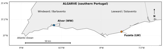
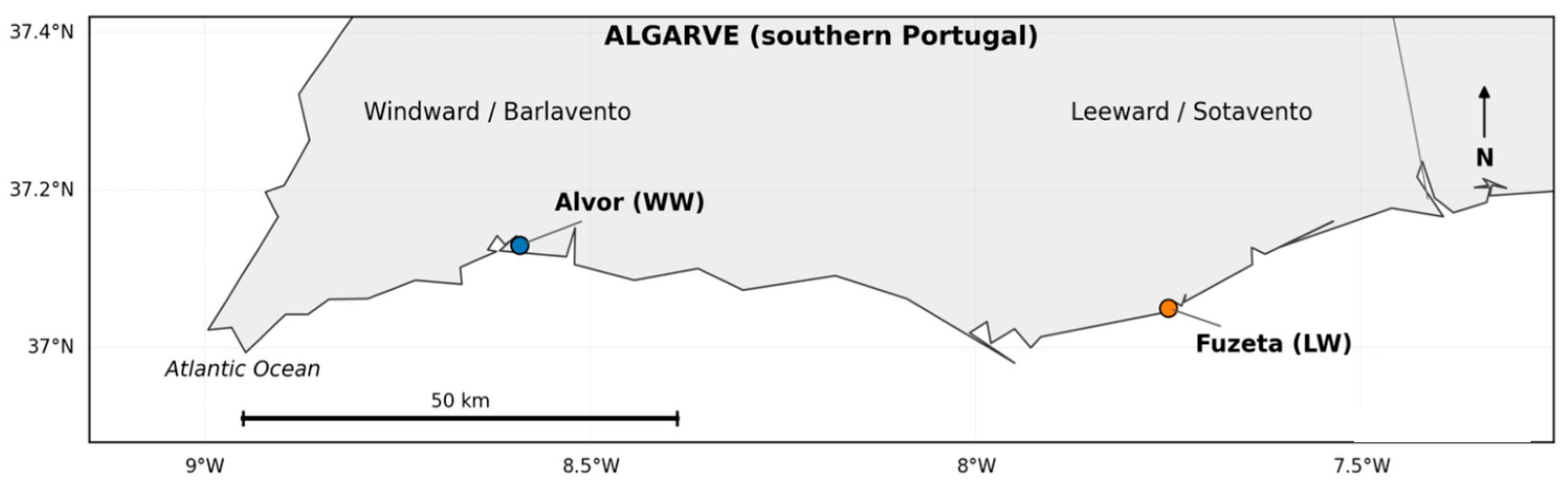
Regional averages are useful descriptors but can conceal operational heterogeneity and dependence on sample composition [14]. At the Algarve, local (up to 9 m vessel length-LOA) and coastal vessels (LOA from 9 to 35 m) differ in operating range, trip duration, carrying capacity and fuel use [9]. The Algarve coast is also commonly divided into Windward/Barlavento (WW) and Leeward/Sotavento (LW) [15]. The western Algarve, represented here by Alvor, is more exposed to Atlantic influence and is generally associated with cooler waters and more rocky or erosional habitats, whereas the eastern Algarve, represented by Fuzeta, has stronger Mediterranean influence, generally warmer coastal waters and a greater prevalence of sandy habitats [15]. These ecological contrasts can be accompanied by differences in prey availability and fishing grounds; however, the WW-LW division is used here as an ecological-operational sampling contrast rather than as a separate management regime. Consequently, unadjusted WW-LW or local/coastal fleet LCA comparisons may simultaneously reflect fleet composition, gear configuration, travelled distance and capture efficiency. Disaggregation by fleet typology and subregion, supported by contribution analysis and explicit uncertainty, is therefore required to avoid simplified causal claims [7,16,17].
Food LCAs also face a functional question. A mass-based functional unit supports production-efficiency assessment and comparison with established fishery literature, but it does not represent the amount and diversity of nutrients supplied [18,19,20]. Nutritional LCA has consequently explored protein, energy and multi-nutrient-based references [21,22,23]. This is relevant for seafood because protein, EPA + DHA, vitamins, selenium, iodine and other micronutrients are supplied together [2,3,18]. The specific gap addressed here is the integration of locally measured multi-nutrient data with environmental LCA for an operationally heterogeneous small-scale fishery while retaining the conventional mass-based reference for interpretation. Nevertheless, the selected nutrient-profile model, reference values, component caps, bioavailability and preparation assumptions influence the result and must be transparent [24,25,26].
The Nutrient Rich Food (NRF) family of indices combines nutrients to encourage with components to limit [27,28]. Based on the local analytical characterization of Algarve octopus [15], this study defined an exploratory NRF17.2-Ov (Octopus vulgaris) containing 17 positive components (protein, EPA + DHA, vitamins B2, B3, B5, B6, B8, B12 and E, magnesium, zinc, copper, selenium, calcium, iodine, potassium and phosphorus) and two limiting components, sodium and saturated fat. The index was used to complement the mass-based functional unit.
Uncertainty is a second central challenge. Differences between means may coexist with broad distributional overlap, and Monte Carlo simulation does not correct sampling imbalance or structural uncertainty [16,29,30]. Environmental and nutritional data may also derive from non-paired observational units. In this study, biological variability refers to real differences among organisms, seasons or locations; parameter uncertainty refers to imperfect knowledge of model inputs or estimated means; and Monte Carlo numerical error refers only to the finite precision of the simulated mean.
The aim of this research was to evaluate the environmental performance and nutrient density of common octopus landed by the Algarve artisanal fleet. Specifically, the study (1) compared the observed WW and LW environmental-nutritional configurations and, secondarily, characterized general, local and coastal environmental scenarios; (2) quantified contributions from diesel, gear and other inventory components; (3) evaluated the robustness of the environmental patterns through contribution analysis and LCIA-method sensitivity; (4) calculated and propagated an exploratory NRF17.2-Ov; and (5) reported impacts both per kg landed and per 100 NRF17.2-Ov points.
2. Materials and Methods
2.1. Case Study, Sampling and Data Quality
The study system was the artisanal common-octopus fishery in the Algarve, Portugal. The subregional comparison included vessels operating from Alvor (WW) and Fuzeta (LW) [15] (Figure 1). Local and coastal SSF fleet categories were assessed as complementary operational typologies. Local SSF boats are smaller and restricted to closer proximity to the shore. The coastal SSF fleet ventures further out to sea; these are larger vessels that undertake longer voyages. The WW-LW comparison was descriptive and was not designed to estimate an isolated causal effect of geography.
Figure 1.
Study-area map showing Alvor (Windward/Barlavento, WW) and Fuzeta (Leeward/Sotavento, LW) on the Algarve coast, Portugal.
The target population consisted of artisanal vessels targeting octopus during 2023. Vessel skippers were contacted through face-to-face interviews. Fishers were opportunistically recruited at fishing harbours and participated voluntarily based on their availability; no random draw from a vessel registry was performed. Eligible vessels reported octopus-directed activity, belonged to the local or coastal category, operated in WW or LW, and could provide annual data on octopus landings, fuel and principal operating inputs. The sample contained 31 vessels: 20 local and 11 coastal; 14 were assigned to WW and 17 to LW (Table 1). The recruitment response rate relative to the complete registered fleet was not available; the sample should therefore be interpreted as an operational convenience sample of Algarve octopus’ vessels.
Table 1.
Distribution of number of participating vessels by subregion and fleet typologies.
Questionnaires covered vessel and engine characteristics, fishing days and hours, distance, typical depth, annual octopus’ landings, fuel, gear use and replacement, bait, salt and maintenance materials. Responses were checked for required variables and unit consistency. Ratios were calculated only when both the relevant annual input and annual octopus’ landings were reported. Potentially inconsistent or outlying entries were traced back to the original questionnaires; observations were retained unless a verifiable transcription, unit or conversion error was identified. Thus, plausibility was not used as an independent statistical exclusion criterion, and no observation was removed solely because its magnitude was high or low. Vessels lacking information for a specific indicator were excluded from that calculation.
2.2. Goal, Scope and Functional References
The study followed ISO 14040 and ISO 14044 [31,32] and adopted an attributional perspective. The cradle-to-port boundary ended at landing and included production, replacement, maintenance and end-of-life modelling of pots, traps, buoys and ropes; fuel supply and combustion; bait; salt; auxiliary consumables; and routine vessel maintenance. Vessel construction and end-of-life were excluded because homogeneous data were unavailable, and their contribution per kg was expected to be comparatively small, consistently with the earlier Algarve study [9].
The principal environmental functional unit was 1 kg of whole octopus landed at the harbour. Annual operating inputs and emissions were attributed in full to reported octopus’ landings. This hypothesis is conservative regarding the absolute catch attributed to octopus when bycatch species were landed, since it was not possible to perform a complete distribution of the mass at the vessel level among all landed species, given that bycatch landings were not systematically reported. This full-attribution rule is homogeneous across vessels but may conservatively overestimate burdens per kg of octopus when secondary species were landed.
A complementary nutritional reference of 100 NRF17.2-Ov points was used. Environmental impacts refer to landed whole octopus, whereas nutrient concentrations refer to 100 g edible portion. The conversion therefore requires an edible-yield factor y, expressed as kg edible portion per kg landed. Because y was not measured in the participating samples, the reported base case uses y = 1.0 as an operational normalization, not as a claim of strict mass equivalence. A sensitivity using y = 0.80 and 0.85, consistent with published octopus-processing ranges, is provided in the Supplementary Material [33]. If a common y is applied to both subregions, absolute normalized impacts change by 1/y, but WW-LW ratios and ordering probabilities do not modify. Different yields by subregion were not evaluated.
2.3. Life-Cycle Inventory and Scenario Construction
Five aggregated foreground models were constructed: global Algarve fleets (GLO), local (LOC), coastal (COA), WW and LW. For each foreground flow, an intensity was calculated separately at vessel level by dividing the annual input by the corresponding annual reported octopus’ landings. Scenario values were subsequently calculated as arithmetic means of the validated vessel-level input-to-landings ratios within each scenario. The resulting aggregated foreground inventory is summarized in Table 2, with further disaggregation provided in the Supplementary Material.
Table 2.
Summary of the foreground inventory and fuel. Inputs are fully attributed to reported octopus’ landings; no mixed-landing mass allocation was applied. Values are mean vessel-level input-to-landings ratios. Data is shown for Algarve fleets (GLO), local (LOC), coastal (COA), Windward (WW), and Leeward (LW).
Fuel-use intensity (FUI) was reconciled from the mass-based diesel inputs. A single diesel density of 0.832 kg/L was applied to every scenario:
where mdiesel,s is the modelled diesel mass per kg landed, and diesel is 0.83 kg/L. This yielded 0.85, 0.71, 1.10, 0.64 and 0.98 L/kg for GLO, LOC, COA, WW and LW, respectively. Direct combustion emissions were recalculated with the Tier 1 fuel-based equation E, = FC × EF using the same factors for all scenarios [34]. The linked background system used ecoinvent 3.11, Allocation, cut-off by classification, in SimaPro 10.2.0.3 [35]. The bait questionnaires reported total annual mass but did not consistently identify bait species, origin or supplier at vessel level. A region- or fleet-specific bait mix could therefore not be reconstructed without introducing unsupported assumptions. Bait was represented by the same generic fish-bait process in every scenario, so only bait quantity per functional unit varied. Gear materials were annualized using installed quantities, declared replacement and loss and assumed service lives of 10 years for pots, 3.5 years for traps and 1 year for ropes.
FUIs = mdiesel,s /ρdiesel
2.4. Life-Cycle Impact Assessment
Environmental Footprint 3.1 V1.03 was the principal LCIA method [36,37]. Characterized midpoint results were retained without normalization, weighting or single-score aggregation. Six indicators were selected for probabilistic interpretation: climate change, acidification, freshwater eutrophication, marine eutrophication, particulate matter and fossil resource use. ReCiPe 2016 Midpoint (H) V1.11 was used as a methodological sensitivity check [38].
2.5. Nutritional Characterization and NRF17.2-Ov
Nutrient data were obtained in the frame of the SEA2SEE project and published previously [15]. Eight composite samples (four per subregion and one per quarter) were prepared from three or four individuals collected between December 2022 and December 2023. Analyses were performed in laboratories operating under UNE-EN ISO/IEC 17025:2017 [15]. Protein was determined by the Kjeldahl method; sodium and minerals, including copper, were measured by ICP-MS after acid digestion; fatty acids were determined by GC-FID after methyl-ester preparation; and vitamins were measured using chromatographic and microbiological methods as detailed in the source study [15]. Nutrient concentrations were reported per 100 g edible portion as means and standard errors of the mean (SEM).
NRF17.2-Ov was defined as an exploratory food-specific indicator for the general adult reference population. All quantified components with an applicable adult reference value and compatibility with the NRF structure were included; selection was not based on the direction of the WW-LW difference. Positive components were capped at 100% of their reference value, whereas sodium and saturated fat were subtracted:
where C is concentration per 100 g, RI is the positive-component reference intake and L is the limiting-component reference.
NRF17.2-Ov = Σi=117 min [100, 100(Ci/RIi)] − Σj=12 100(Cj/Lj)
EU reference intakes were used for protein, saturated fat, vitamins and minerals [39]; 250 mg/day for EPA + DHA was taken from EFSA [40] and 2000 mg/day for sodium from WHO [41]. Vitamins B1 and B9 were excluded because concentrations were below the limit of quantification [15]. Saturated fat, reported as <0.1 g/100 g, was conservatively set to 0.10 g/100 g with SEM = 0. The index is not a complete-diet assessment.
2.6. Environmental-Nutritional Conversion
Impact100NRF= Impactkg,landed × 10/(NRF17.2-Ov × y)
The factor 10 converts the score per 100 g to a kg basis, and y is edible yield. The main results use y = 1.0 to preserve the operational normalization used in the original model.
2.7. Parameterized Environmental and Nutritional Uncertainty
Parameterized environmental uncertainty was propagated for WW and LW with the SimaPro Monte Carlo module. For each foreground flow, the SEM of the vessel-level input-to-landings ratio was calculated as follows:
where SD(r) is the sample standard deviation of the validated vessel-level input-to-landings ratios, and n is the number of vessels with valid observations for the corresponding flow and scenario.
SEMr = SD(r)/√n
Normal foreground distributions were centered on the scenario-specific inventory quantities. These distributions were modelling assumptions used to propagate parameter uncertainty; no formal normality or goodness-of-fit test was used to infer the underlying vessel-level population distribution. Only four foreground flows were assigned uncertainty distributions in each zonal model: diesel, bait, pots and traps. For diesel, the uncertainty distribution was assigned to the technosphere fuel-supply input. Direct combustion elementary flows, calculated from the scenario-specific central fuel consumption using Tier 1 emission factors, were retained at their deterministic central values during the Monte Carlo simulations. For WW, the reported triplets (central value/SEM used as SD/SimaPro 2 × SD input) were 0.53/0.17/0.34 kg/kg for diesel, 1.02/0.20/0.40 kg/kg for bait, 0.38/0.03/0.06 kg/kg for pot assemblies and 0.24/0.03/0.06 kg/kg for trap assemblies. For LW, the corresponding triplets were 0.81/0.17/0.34, 0.70/0.13/0.26, 0.31/0.03/0.07 and 0.45/0.02/0.04 kg/kg, respectively. All other foreground flows were kept deterministic. Background uncertainty came from linked ecoinvent 3.11 unit-process distributions.
One thousand environmental iterations were exported per zone and indicator. Means, medians, sample SDs, coefficients of variation and empirical 2.5th–97.5th percentiles were calculated. The SD and percentile range describe the simulated distribution. SD/√1000, is labelled Monte Carlo error of the simulated mean and is not interpreted as production-system uncertainty.
Nutritional uncertainty was propagated through 1000 profiles per zone. Each concentration was sampled from a normal distribution with mean equal to the published concentration and SD equal to the SEM, left-censored at zero. Nutrients with SEM = 0 were constant. Nutrients were treated as independent because covariance data were unavailable. With four samples per zone, this model represents uncertainty in the reported zonal mean rather than full biological variability. The analysis was intentionally restricted to the published means and SEMs. The resulting distributions should therefore be interpreted as a parametric approximation to uncertainty in the zonal means. Consequently, the nutritional Monte Carlo analysis should be interpreted as a propagation of uncertainty parameterized under the established assumptions.
2.8. Probability-of-Superiority Comparison
The unpaired probability P (LW > WW) was calculated from all 1000 × 1000 cross-combinations of the two empirical marginal distributions. An unpaired construction was used because the WW and LW simulations represent separate marginal scenarios, and there is no vessel-level or nutritional-sample pairing that would justify matching iteration in one zone with iteration in the other. The estimator therefore answers whether a random LW outcome exceeds an independently selected WW outcome under the modelled marginal distributions; it is not a p-value and does not represent a paired LW-WW distribution [17,29,30]. Ratios and differences were evaluated analogously. The cross-combinations increase numerical resolution of the empirical comparison but do not create additional independent observations.
The local-coastal comparison was retained as a secondary deterministic analysis and was not assigned a probability of superiority. Likewise, no hypothesis test was applied to the deterministic NRF17.2-Ov score difference; uncertainty in the zonal nutritional comparison was evaluated through the Monte Carlo distributions and P (NRFLW > NRFWW).
3. Results
3.1. Sample Structure and Fuel Use
FUI was 0.85 L/kg for the overall Algarve configuration, 0.71 L/kg for local vessels and 1.10 L/kg for coastal vessels, a 1.56-fold difference (approximately 56% higher in coastal). WW and LW values were 0.64 and 0.98 L/kg. Fleet composition was asymmetric: local vessels represented 78.6% of WW and 52.9% of LW, while coastal vessels represented 21.4% and 47.1%, respectively. The local-coastal FUI contrast is reported descriptively.
3.2. Environmental Profile
The local and coastal models did not show a uniform environmental ordering across the 25 reported EF 3.1 indicators, including climate-change and toxicity sub-indicators. Coastal exceeded local in seven reported indicators, whereas local exceeded coastal in 18 (Supplementary Table S5). Across the six priority indicators, coastal was higher for climate change, marine eutrophication, particulate matter and fossil-resource use by 19.0%, 40.8%, 13.6% and 12.3%, respectively. Local had very slightly higher acidification (0.0073 vs. 0.0072 mol H+ eq/kg) and twice the freshwater eutrophication (2.30 × 10⁻⁴ vs. 1.15 × 10⁻⁴ kg P eq/kg). Climate-change impacts were 3.26 kg CO2 eq/kg for local and 3.88 kg CO2 eq/kg for coastal, compared with the global result of 3.47 kg CO2 eq/kg (Table 3).
Table 3.
Deterministic Environmental Footprint 3.1 results per kg of octopus landed. Windward (WW) and Leeward (LW) are aggregated configurations with unequal fleet composition. Results do not estimate an adjusted effect of subregion. Data is shown for Algarve fleets (GLO), local (LOC), coastal (COA), Windward (WW) and Leeward (LW).
LW exceeded WW in 24 of the 25 reported EF indicators; ozone depletion was 8.5% lower in LW. For the six selected indicators, deterministic LW-WW differences ranged from 22.9% for fossil-resource use to 51.1% for marine eutrophication.
ReCiPe 2016 Midpoint (H) confirmed the absence of a uniform local-coastal ordering. Coastal values exceeded local values across six of the 18 ReCiPe indicators. Global warming was 3.33 kg CO2 eq/kg for local and 3.96 kg CO2 eq/kg for coastal, a difference of 18.9%. Unlike EF 3.1, ReCiPe terrestrial acidification was higher in coastal, while marine eutrophication was higher in local, showing dependence on the LCIA method. LW exceeded WW across all 18. For conceptually comparable indicators, LW-WW differences were 42.4% for global warming, 47.2% for fine particulate-matter formation, 47.4% for terrestrial acidification, 33.9% for freshwater eutrophication and 23.0% for fossil-resource scarcity (Supplementary Table S6).
3.3. Contribution Profiles
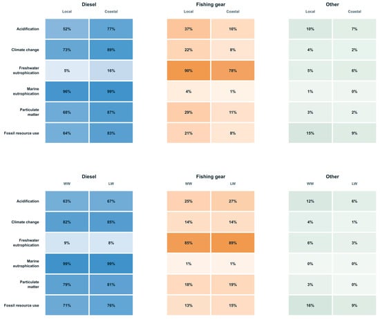
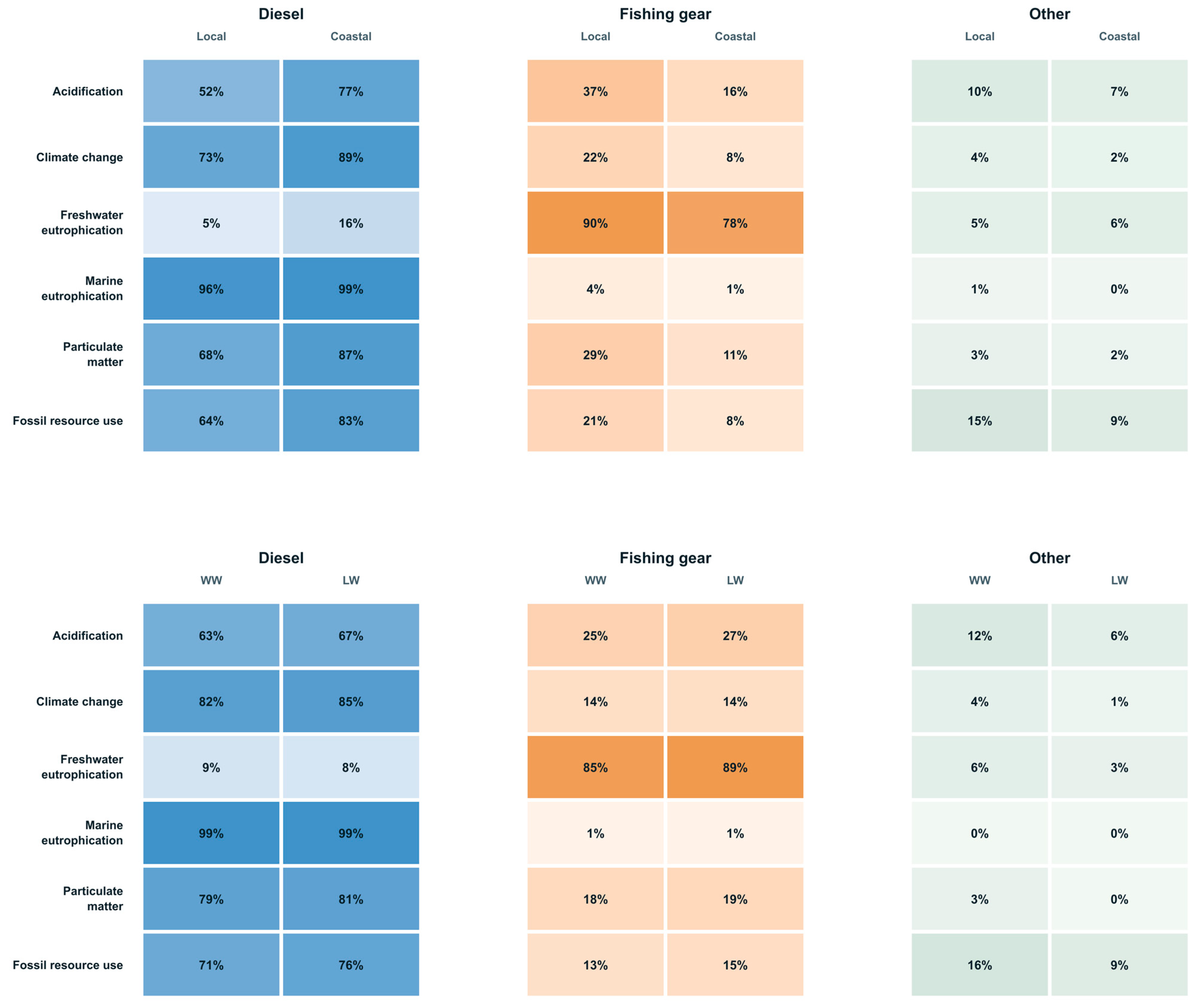
The foreground inventory showed contrasting operational profiles. Diesel dominated climate change, marine eutrophication, particulate matter and fossil-resource use (Figure 2).
Figure 2.
Environmental relative contribution heatmap (%) of diesel, fishing gear and other processes in (top) local and coastal fleet typologies and (bottom) observed WW and LW configurations. Darker shading indicates a larger contribution. WW: Windward; LW: Leeward.
Coastal used more diesel per kilogram landed (0.917 vs. 0.587 kg/kg), whereas local used more bait (1.019 vs. 0.676 kg/kg), pot assembly (0.531 vs. 0.205 kg/kg), trap assembly (0.566 vs. 0.256 kg/kg) and buoy and line assembly (0.082 vs. 0.034 kg/kg).
For the WW and LW configurations, diesel remained the principal contributor to climate change and shared the main energy-related hotspots. Diesel contributed 82% and 85% of climate change and >95% of marine eutrophication. Freshwater eutrophication followed a different pattern and reflected the contrasting mix of pots and traps between the two subregional configurations.
3.4. Environmental Uncertainty and the WW-LW Comparison
Monte Carlo means were consistent with deterministic results. The reported dispersion reflects the stochastic parameters included in the model and should not be interpreted as complete uncertainty of the environmental system. Dispersion varied markedly by indicator: freshwater eutrophication had CVs of 54.3% in WW and 53.0% in LW, followed by fossil-resource use at 30.0% and 25.3%. Marine eutrophication had CVs close to 1%.
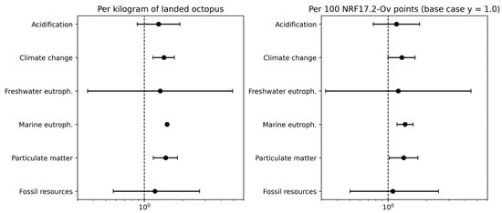
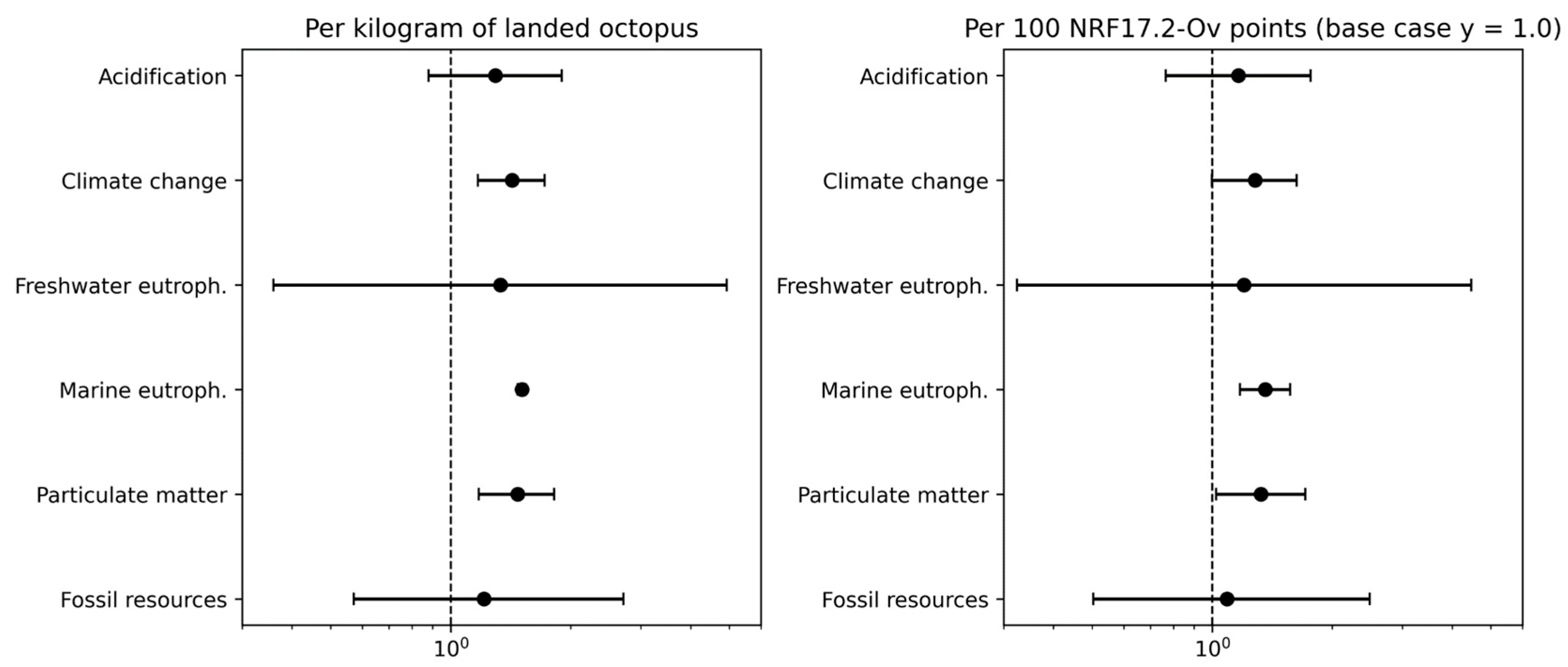
Under the unpaired independence assumption, LW means exceeded WW means by 29.5% for acidification, 42.6% for climate change, 33.3% for freshwater eutrophication, 51.0% for marine eutrophication, 47.3% for particulate matter and 21.2% for fossil-resource use. Under the specified Monte Carlo parameterization, the probability of a higher LW impact was >0.99 for climate change, marine eutrophication and particulate matter. Acidification had a probability of 0.91 but a ratio interval crossing one. Evidence was weaker for freshwater eutrophication (0.67) and fossil-resource use (0.70) (Table 4 and Figure 3).
Table 4.
Monte Carlo summary and unpaired Leeward-Windward (LW-WW) comparison per kg of landed octopus. Probabilities and ratio intervals were calculated from all cross-combinations of 1000 marginal outcomes per zone. Cross-combinations are not independent Monte Carlo observations.
Figure 3.
Unpaired Leeward/Windward (LW/WW) impact ratios from the marginal Monte Carlo distributions: (left) per kg of landed octopus and (right) per 100 NRF17.2-Ov points in the operational base case y = 1.0. Points are ratios of marginal means; bars are empirical 2.5th–97.5th percentiles of all cross-combinations. The dashed reference line indicates equality LW/WW = 1 in log scale.
3.5. NRF17.2-Ov Nutrient Density
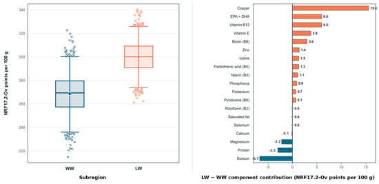
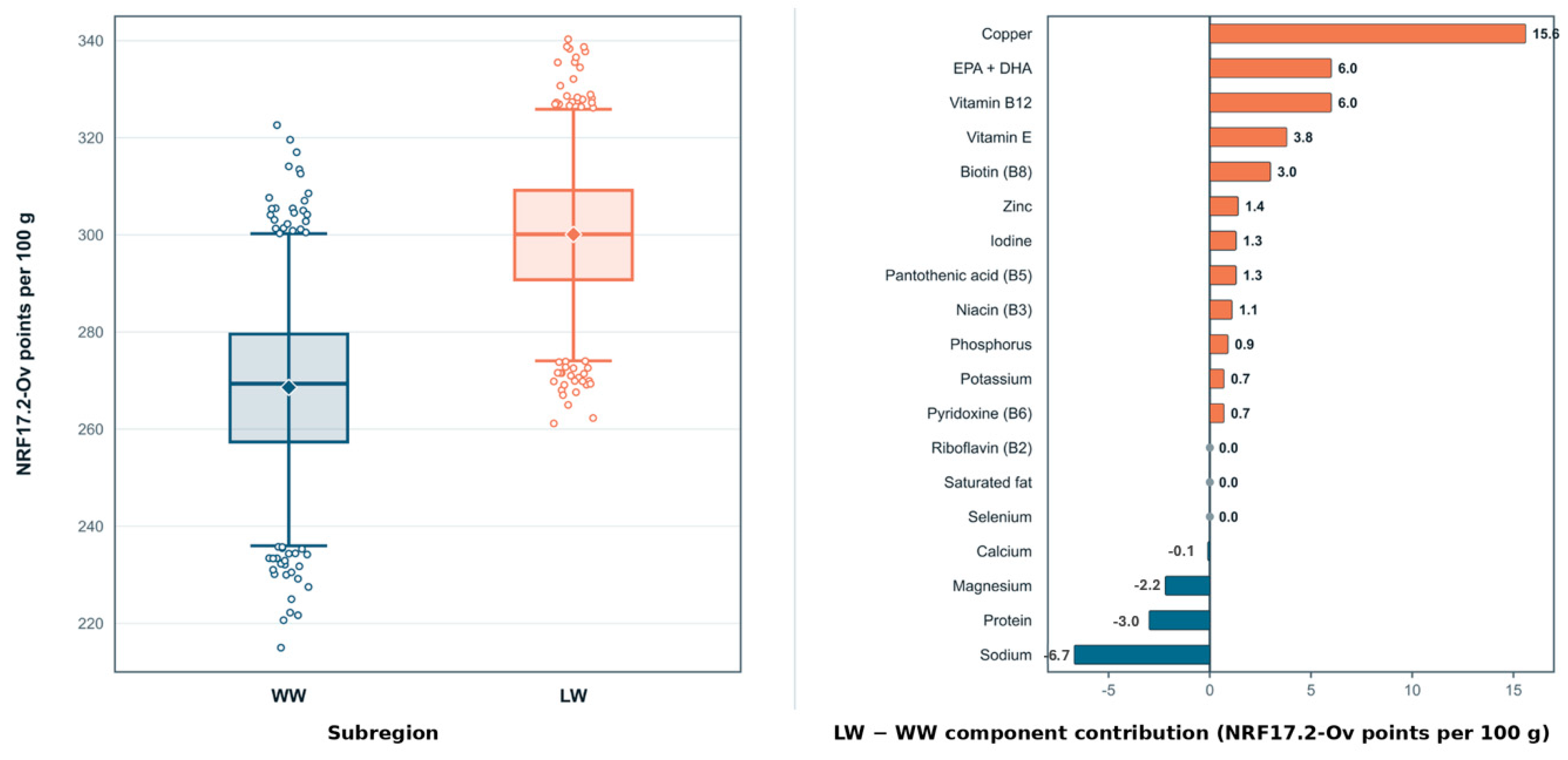
Deterministic NRF17.2-Ov was 269.3 points for WW and 299.3 for LW, an 11.1% difference. Positive-component sums were 284.4 and 321.0, partly offset by limiting-component penalties of 15.08 and 21.75. Monte Carlo means were 269.4 and 299.3, respectively. No hypothesis test was applied to the arithmetic difference between the two deterministic scores. Under the specified uncertainty model, the unpaired probability of a higher LW score was 0.93, although the empirical intervals overlapped. Copper was the largest contributor to the LW-WW difference (+15.6 points), followed by EPA+DHA (+6.0), vitamin B12 (+6.0), vitamin E (+3.8) and biotin (+3.0). These gains were partly offset by a larger sodium penalty in LW (−6.7 points relative to WW) and lower protein (−3.0) and magnesium (−2.2) contributions (Figure 4 and Table 5).
Figure 4.
Nutritional performance: (left) Monte Carlo distribution of NRF17.2-Ov by subregion; (right) deterministic Leeward-Windward (LW-WW) difference in each component contribution. Positive values favor LW; negative values favor WW or indicate a larger limiting-component penalty in LW.
Table 5.
Deterministic and Monte Carlo NRF17.2-Ov results. LIM2 is the combined sodium and saturated-fat penalty. P (NRFLW > NRFWW) = 0.93. kg/100 NRF values are operational base-case values with y = 1.0. Windward: WW, Leeward: LW.
3.6. Impacts per 100 NRF17.2-Ov Points
Under the operational base case y = 1.0, the mass required to provide 100 NRF17.2-Ov points was 0.037 kg for WW and 0.033 kg for LW. Nutritional normalization reduced the relative LW-WW environmental difference by approximately 12–15 percentage points without reversing the mean ordering. The remaining difference ranged from 9.0% for fossil-resource use to 35.8% for marine eutrophication.
The probability of a higher LW impact remained >0.99 for marine eutrophication and 0.98 for particulate matter. For climate change, it decreased to 0.97. Acidification, freshwater eutrophication and fossil-resource use had probabilities of 0.78, 0.61 and 0.60, respectively (Table 6).
Table 6.
Monte Carlo impacts per 100 NRF17.2-Ov points in the operational base case y = 1.0. If the same edible yield is applied to Windward (WW) and Leeward (LW), all absolute values are multiplied by 1/y, while ratios and probabilities remain unchanged.
4. Discussion
4.1. Operational Heterogeneity and Fleet Typology
Within the observed sample, a single aggregated Algarve value concealed substantial operational heterogeneity, but the results do not support a simple environmental hierarchy between local and coastal vessels. FUI was 0.706 L/kg in local and 1.102 L/kg in coastal, approximately 56% higher in the coastal configuration, while local had substantially higher catch-normalized bait and gear inputs. Accordingly, coastal exceeded local in seven of the 25 reported EF 3.1 indicators, whereas local exceeded coastal in 18. These counts include sub-indicators and do not establish overall environmental superiority. The local-coastal comparison remains descriptive and deterministic. Because scenario values are arithmetic means of vessel-level intensities, they describe the mean observed vessel rather than the footprint of the fleet’s total landed production; a landings-weighted regional footprint could therefore differ.
The overall climate-change result of 3.47 kg CO2 eq /kg is close to the approximately 3.1 kg CO2 eq /kg previously reported for the Algarve fishery [9]. Disaggregation yielded 3.26 kg CO2 eq/kg in local and 3.88 kg CO2 eq/kg in coastal, a 19.0% difference.
The smaller contrast in climate change than in FUI is consistent with the higher catch-normalized bait and gear inputs in local fisheries offsetting part of its fuel advantage. Fuel intensity therefore needs to be interpreted alongside other operational inputs. This supports the broader fishery-LCA finding that catch efficiency and fuel intensity can generate differences within a fishery that are comparable with differences between fishing systems [6,7,8]. Directly comparable published FUI benchmarks for small-scale octopus fisheries remain scarce. Almeida et al. [9], working on the Algarve small-scale fishery with a different analytical focus, reported an FUI near 0.9 L/kg, close to the overall FUI of 0.85 L/kg reported here. By contrast, the Mauritanian octopus LCA assessed industrial trawlers with onboard processing and freezing [13] and is not an operationally equivalent small-scale benchmark. The present results therefore provide useful within-fishery disaggregation but should not be interpreted as a generalized Atlantic or Mediterranean FUI range.
4.2. Environmental Hotspots and WW-LW Comparison
Diesel dominated indicators connected to combustion and energy, consistent with fishery-LCA literature [7,8,9]. FUI is therefore the principal operational metric for climate change, marine eutrophication, particulate matter and fossil resources. Potential routes to lower FUI include reduced fuel consumption, higher catch per trip, fewer low-yield trips, route planning and changes in deployment strategy; these options were not tested directly in the present study. These measures require attention to safety, stock status and unintended effort displacement.
Freshwater eutrophication showed that fuel efficiency alone cannot improve every indicator. Gear manufacture and replacement accounted for most of this indicator, and gear also contributed materially to acidification and particulate matter in local. Pot and trap assembly intensities in local vessels were approximately 2.6 and 2.2 times those in coastal vessels, respectively, consistent with the higher freshwater-eutrophication result observed for local vessels. Increasing service life, reducing loss, improving recovery and considering material substitutions are therefore relevant [9,11,12]. However, extending service life is not automatically beneficial if ageing gear increases repair requirements, loss risk or reduces fishing efficiency, whereas premature replacement creates additional embodied material impacts. The appropriate strategy is therefore to optimize service life jointly with catch efficiency, repair, loss and recovery rather than to maximize durability in isolation.
Bait contributed most visibly to fossil-resource use. Alternative bait sourcing could alter absolute results and category trade-offs, but no substitution should be considered beneficial without evaluating catch efficiency, selectivity, supply-chain burdens and possible changes in bait quantity.
WW and LW shared the same principal hotspots, although LW showed higher absolute impacts for most indicators. However, the groups were not balanced: WW was dominated by local vessels, whereas LW contained almost equal local and coastal representation. The observed contrast may therefore reflect FUI, fleet category, gear mix, distance, trip duration and catch efficiency as well as subregion. Monte Carlo simulation propagates assigned parameter uncertainty; it cannot remove fleet-composition confounding, correct convenience-sampling bias or account for unmeasured variables [16,17]. Consequently, the reported WW-LW probabilities are conditional on the specific sample composition and model structure and must not be interpreted as probabilities of a true geographical effect.
The probability-of-superiority results are best interpreted hierarchically. Climate change, marine eutrophication and particulate matter showed strong separation between the modelled marginal distributions. Acidification, freshwater eutrophication and fossil resources had wider overlaps. None of these probabilities proves a geographical mechanism, and the one million cross-combinations do not constitute one million independent observations. Because WW included only three coastal vessels and the four fleet-by-subregion strata were not independently parameterized, an adjusted within-typology geographical comparison was not estimated.
4.3. Nutrient Density and Functional Normalization
The higher LW NRF17.2-Ov is consistent with the analytical differences reported for Algarve octopus [15]. The exploratory index includes the complete available set of compatible measured nutrients rather than a post hoc subset selected to favor either zone [21,42,43]. It broadens nutritional representation beyond protein or energy alone, but its outcome remains dependent on reference values, positive-component caps and limiting-component rules [25,26,27]. Copper was particularly influential because the measured concentrations were 2.17 mg/kg in WW and 3.73 mg/kg in LW [15], which translate directly into approximately 21.7 and 37.3 NRF points per 100 g using the EU reference intake of 1 mg [39]. Importantly, the underlying nutritional study reported no statistically significant WW-LW difference for the mineral and vitamin measurements and cautioned against overinterpreting the small-sample differences [15]. The present dataset therefore cannot establish whether the Cu contrast arose from prey, substrate, water chemistry, bioaccumulation or analytical variability. NRF17.2-Ov treats Cu as an essential nutrient and does not invalidate a toxicological-risk index.
The higher sodium penalty in LW illustrates why positive and limiting components should be presented together. NRF17.2-Ov does not represent an entire diet and does not model bioavailability, digestibility, cooking retention or individual requirements [23,24,26].
Nutritional normalization reduced but did not eliminate the observed environmental gap. This supports treating nutrient density and environmental intensity as complementary dimensions rather than interchangeable rankings [18,20,24]. The edible-yield issue is important: landed whole mass and edible portion are different reference flows. Because the edible-yield factor y was not measured, the y = 1.0 values should be read as operational normalizations. Within this WW-LW comparison, applying the same y to both zones multiplies absolute normalized impacts by 1/y but leaves the WW-LW ratios and ordering probabilities unchanged. Across different seafood species, product forms or processing methods, however, edible yield can differ substantially; using product-specific yields could therefore change nutrition-normalized comparisons. Consumer-level dietary applications would additionally require measured edible yield and, where relevant, nutrient retention after preparation rather than the common y operational assumption used here.
4.4. Uncertainty, Limitations and Reproducibility
The combined deterministic, Monte Carlo, method-sensitivity and nutrient-normalization results provide a structured robustness assessment, but uncertainty coverage remains incomplete. Foreground distributions were centred on vessel-level mean intensities and were used as parametric uncertainty representations more precisely than fitted biological or fleet-population distributions. No formal normality test was used to establish an underlying population distribution. This approximation does not account for covariance between inputs and landings and does not fully capture inter-vessel variability. Background distributions were obtained from ecoinvent and do not address model structure, alternative datasets, allocation choices, annual variation, bait origin or gear-loss scenarios. In addition, uncertainty assigned to diesel consumption was applied to the technosphere fuel-supply input, whereas the direct Tier 1 combustion elementary flows were retained at their scenario-specific deterministic central values. Fuel-related uncertainty was therefore only partially propagated. This modelling choice particularly affects the interpretation of distribution width for impact categories strongly influenced by direct combustion emissions. Accordingly, narrow Monte Carlo distributions should not be interpreted as evidence of low total production-system uncertainty.
Nutritional simulation was based on four composite samples per zone. A normal distribution parameterised with the SEM approximates uncertainty in the reported mean, not a representation of biological variability among individual octopuses. The analysis intentionally used the published means and SEMs and did not reanalyse the four original observations. This modelling choice should be considered when interpreting the width of the nutritional distributions and the probability of a higher NRF17.2-Ov score.
Other limitations include voluntary recruitment, unknown response rate, a single reference year, self-reported annual activity, incomplete secondary-landings data, full attribution to octopus, generic bait modelling, assumed gear lifetimes, absence of a measured edible yield and lack of independent inventory estimates for the four fleet-by-subregion strata. Because recruitment was opportunistic and the study did not record comparable characteristics for non-participants, the direction of any participation bias (i.e., whether participants were systematically larger, more efficient or more environmentally engaged) cannot be determined. A non-participant sensitivity analysis was not performed because no empirical distribution for non-participants was available; imposing an arbitrary alternative distribution would add unsupported assumptions. Likewise, the very small WW coastal stratum (n = 3) limits any attempt to remove fleet-composition effects by comparing fully balanced local-only or coastal-only geographical strata. The assessment also does not include stock status, by-catch, benthic disturbance, ghost fishing or plastic leakage as characterized LCA indicators [7,9,12]. Additionally, lower climate impact is not equivalent to comprehensive fishery sustainability.
4.5. Management, Climate Context and Traceability Implications
For operational improvement, the two fleet typologies point to different priorities within the observed sample. The coastal configuration should first target fuel-use intensity through trip planning, catch efficiency and other measures that reduce fuel per kilogram landed without displacing effort or compromising safety. The local configuration, which showed higher catch-normalized bait and gear inputs and higher freshwater eutrophication, should place greater emphasis on gear service life, loss prevention, recovery, material efficiency and bait traceability. Should a traceability system for Algarve octopus be developed, recording fleet category, subregion, gear type, fuel use, trip distance or duration, total and octopus’ landings, bait quantity and origin and gear use, replacement and loss could support environmental performance ranges rather than a single fixed footprint. Climate change adds a further longitudinal uncertainty: shifts in water temperature, prey fields, octopus’ distribution or seasonality could modify catch rates and therefore FUI and gear effort, while temperature and diet-related changes may also affect nutritional composition [15]. The single-year environmental inventory and one-year nutritional sampling cannot quantify the direction or magnitude of these future changes, so repeated multi-year monitoring would be required. Environmental and nutritional information should complement, rather than replace, stock, social and economic indicators and should not be interpreted or aggregated as a single measure of overall fishery sustainability [1,20,44].
5. Conclusions
The results showed substantial environmental heterogeneity across the modelled operational configurations. Fuel-use intensity was 0.71 L/kg for local vessels and 1.10 L/kg for coastal vessels, with diesel use being the main driver of climate change, marine eutrophication, particulate matter and fossil-resource use. However, impacts were not exclusively fuel-driven, as fishing-gear production and replacement were important contributors to other impact categories, particularly freshwater eutrophication. Within the observed configurations, coastal operators therefore have a clearer fuel-efficiency priority, whereas local operators have a stronger gear-durability, recovery, material-efficiency and bait-traceability priority. These are configuration-specific improvement directions rather than claims that one fleet type is environmentally superior overall.
The observed LW configuration showed higher mean environmental impacts than WW for most indicators and a higher NRF17.2-Ov score. Nutritional normalization reduced the magnitude of the environmental difference but did not reverse the ordering of marine eutrophication or particulate matter. These results are descriptive: WW and LW had unequal fleet composition, recruitment was non-probabilistic, and the analysis cannot isolate a geographical effect.
The results identify fuel-use intensity and gear durability as key drivers of environmental performance within the assessed operational configurations. Future validation should combine stratified sampling by fleet typology and subregion with repeated seasonal or annual vessel-level fuel and landing records, preferably from logbooks or direct fuel monitoring, and direct recording of gear age, replacement, repair, loss and recovery. Material-resolved contribution analysis and sensitivity testing of gear service life would then allow the freshwater-eutrophication hotspot to be tested more directly, while improved bait-species traceability and measured edible yield would strengthen the environmental and nutritional interpretation.
Supplementary Materials
The following supporting information can be downloaded at https://www.mdpi.com/article/10.3390/su182010564/s1, Figure S1: Monte Carlo distributions of NRF17.2-Ov for WW and LW (1000 iterations per zone). Dashed lines indicate simulated means. WW: Windward fleet; LW: Leeward fleet; Figure S2: Contributions of the 19 components to NRF17.2-Ov (in points) in WW and LW. WW: Windward fleet; LW: Leeward fleet; Figure S3: Pearson correlation coefficient between each simulated component and final NRF17.2-Ov. This sensitivity reflects component uncertainty and model rules, not causal biological influence; Figure S4a: Monte Carlo distribution of acidification per kilogram of octopus landed in WW and LW. WW: Windward fleet; LW: Leeward fleet; Figure S4b: Monte Carlo distribution of climate change per kilogram of octopus landed in WW and LW. WW: Windward fleet; LW: Leeward fleet; Figure S4c: Monte Carlo distribution of freshwater eutrophication per kilogram of octopus landed in WW and LW. WW: Windward fleet; LW: Leeward fleet; Figure S4d: Monte Carlo distribution of marine eutrophication per kilogram of octopus landed in WW and LW. WW: Windward fleet; LW: Leeward fleet; Figure S4e: Monte Carlo distribution of particulate matter per kilogram of octopus landed in WW and LW. WW: Windward fleet; LW: Leeward fleet; Figure S4f: Monte Carlo distribution of fossil resource use per kilogram of octopus landed in WW and LW. WW: Windward fleet; LW: Leeward fleet; Figure S5: Unpaired LW/WW ratios per octopus kilogram landed; ratio distributions using 1000 × 1000 combinations per fleet. Points show ratios of marginal means; bars show the empirical cross-combination interval. Intervals and probabilities use all combinations. Violin: empirical convolution density; thick line: interquartile range; dot: ratio of means. WW: Windward fleet; LW: Leeward fleet; Figure S6: Unpaired LW/WW ratios per 100 NRF17.2-Ov points in the y = 1.0 base case. Environmental impacts and NRF-normalized masses are combined on the log scale and treated as independent. Violin: empirical convolution density; thick line: interquartile range; dot: ratio of means. WW: Windward fleet; LW: Leeward fleet; Figure S7: Unpaired probability that a randomly selected LW fleet outcome exceeds a randomly selected WW fleet outcome, per kilogram and per 100 NRF points. Green bars: per kg of octopus; Orange bars: per 100 NRF points. WW: Windward; LW: Leeward; Figure S8: Relative contributions of diesel, fishing gear and other processes to six Environmental Footprint 3.1 indicators selected for local (LOC) and coastal (COA) fleet typologies. GLO: global; Figure S9: Relative contributions of diesel, fishing gear and other processes to six Environmental Footprint 3.1 indicators selected for observed Windward (WW) and Leeward (LW) configurations. GLO: global; Table S1: Reference values used in NRF17.2-Ov; Table S2: Monte Carlo summary of NRF17.2-Ov. The Monte Carlo error of the mean is SD/√1000 and quantifies numerical precision of the simulated mean; it is not biological variability or production-system uncertainty. P (NRF_LW > NRF_WW) = 0.93; Table S3: Contribution of the 17 positive and 2 limiting components to NRF17.2-Ov. WW: Windward fleet; LW: Leeward fleet; Table S4: Descriptive statistics of environmental Monte Carlo distributions. MC error = SD/√1000. Empirical P2.5-P97.5 intervals describe the simulated distributions and should not be confused with confidence intervals of the mean; Table S5: Complete deterministic Environmental Footprint 3.1 results per kilogram landed; Table S6: Complete deterministic ReCiPe 2016 Midpoint (H) results per kilogram landed; Table S7: Calculation of mass-based diesel inventory and volumetric fuel-use intensity; Table S8: Available GLO, LOC, COA, WW and LW foreground inventory per kilogram landed; Table S9: Available gear-material inventory for GLO, LOC, COA, WW and LW; Table S10: Available vessel-maintenance inventory; Table S11: Foreground uncertainty parameterization used in the WW and LW models; Table S12: Sensitivity of selected nutritionally normalized impacts to a common edible-yield factor.
Author Contributions
D.B.d.S. conceptualization, methodology, formal analysis, investigation, data curation, writing—original draft preparation, review and editing; A.G.C. investigation, validation, writing—review and editing, funding acquisition; J.P. investigation; and M.R. investigation, writing—review and editing, funding acquisition. All authors have read and agreed to the published version of the manuscript.
Funding
This research was conducted within the Sea2See project, funded by the European Union’s Horizon Europe research and innovation program under grant agreement No. 101060564. This study received Portuguese national funds from FCT-Foundation for Science and Technology through contracts UID/04326/2025 (DOI: 10.54499/UID/04326/2025), UID/PRR/04326/2025 (DOI: 10.54499/UID/PRR/04326/2025) and LA/P/0101/2020 (DOI: 10.54499/LA/P/0101/2020).
Institutional Review Board Statement
Octopus specimens were collected between December 2022 and December 2023, while the questionnaires were developed between July and December 2024. The study was conducted, in accordance with the Declaration of Helsinki and approved by the Ethics Committee of University of the Algarve (protocol code CEUAlg Pnº 40/2024 and 4 July 2024 of approval).
Informed Consent Statement
Informed consent was obtained from all subjects involved in the study.
Data Availability Statement
The original contributions presented in this study are included in the article and Supplementary Materials. Further inquiries can be directed at the corresponding author.
Acknowledgments
The authors acknowledge the participating fishers, Docapesca and the Sea2See consortium.
Conflicts of Interest
The authors declare no conflict of interest.
Abbreviations
The following abbreviations are used in this manuscript:
| WW | Windward |
| LW | Leeward |
| LCIA | Life Cycle Impact Assessment |
| GLO | global Algarve fleets |
| LOC | local fleet |
| COA | coastal fleet |
| FUI | fuel-use intensity |
| NRF | nutrient-rich food |
| EF | environmental footprint |
References
- de Sousa, D.B.; Vázquez-Rowe, I.; Kahhat, R. Main challenges for measuring the sustainability of the marine ingredients industry: A systematic and critical review. Aquaculture 2026, 613, 743287. [Google Scholar] [CrossRef] [Scilit]
- Venugopal, V.; Gopakumar, K. Shellfish: Nutritive value, health benefits, and consumer safety. Compr. Rev. Food Sci. Food Saf. 2017, 16, 1219–1242. [Google Scholar] [CrossRef] [Scilit] [PubMed]
- Tacon, A.G.J. Contribution of fish and seafood to global food and feed supply: An analysis of the FAO Food Balance Sheet for 2019. Rev. Fish. Sci. Aquac. 2023, 31, 274–283. [Google Scholar] [CrossRef] [Scilit]
- Vázquez-Rowe, I.; Hospido, A.; Moreira, M.T.; Feijóo, G. Best practices in life cycle assessment implementation in fisheries: Improving and broadening environmental assessment for seafood production systems. Trends Food Sci. Technol. 2012, 28, 116–131. [Google Scholar] [CrossRef] [Scilit]
- Ruiz-Salmón, I.; Laso, J.; Margallo, M.; Villanueva-Rey, P.; Rodríguez, E.; Quinteiro, P.; Dias, A.C.; Almeida, C.; Nunes, M.L.; Marques, A.; et al. Life cycle assessment of fish and seafood processed products—A review of methodologies and new challenges. Sci. Total Environ. 2021, 761, 144094. [Google Scholar] [CrossRef] [Scilit] [PubMed]
- Parker, R.W.R.; Tyedmers, P.H. Fuel consumption of global fishing fleets: Current understanding and knowledge gaps. Fish. Fish. 2015, 16, 684–696. [Google Scholar] [CrossRef] [Scilit]
- Avadí, A.; Fréon, P. Life cycle assessment of fisheries: A review for fisheries scientists and managers. Fish. Res. 2013, 143, 21–38. [Google Scholar] [CrossRef] [Scilit]
- Parker, R.W.R.; Blanchard, J.L.; Gardner, C.; Green, B.S.; Hartmann, K.; Tyedmers, P.H.; Watson, R.A. Fuel use and greenhouse gas emissions of world fisheries. Nat. Clim. Change 2018, 8, 333–337. [Google Scholar] [CrossRef] [Scilit]
- Almeida, C.; Loubet, P.; Laso, J.; Nunes, M.L.; Marques, A. Environmental assessment of common octopus (Octopus vulgaris) from a small-scale fishery in Algarve (Portugal). Int. J. Life Cycle Assess. 2022, 27, 849–867. [Google Scholar] [CrossRef] [Scilit]
- Rangel, M.; Pita, C.; Oliveira, M.M.; Guimarães, M.H.; Rainha, R.; Sonderblohm, C.; Monteiro, P.; Oliveira, F.; Ballesteros, M.; Gonçalves, J.M.S.; et al. Do fisher associations really represent their members’ needs and opinions? The case study of the octopus fishery in the Algarve (south Portugal). Mar. Policy 2019, 101, 276–284. [Google Scholar] [CrossRef] [Scilit]
- Erzini, K.; Bentes, L.; Coelho, R.; Lino, P.G.; Monteiro, P.; Ribeiro, J.; Gonçalves, J.M.S. Catches in ghost-fishing octopus and fish traps in the northeastern Atlantic Ocean (Algarve, Portugal). Fish. Bull. 2008, 106, 321–327. [Google Scholar]
- Loulad, S.; Houssa, R.; Rhinane, H.; Boumaaz, A.; Benazzouz, A. Spatial distribution of marine debris on the seafloor of Moroccan waters. Mar. Pollut. Bull. 2017, 124, 303–313. [Google Scholar] [CrossRef] [Scilit] [PubMed]
- Vázquez-Rowe, I.; Moreira, M.T.; Feijóo, G. Environmental assessment of frozen common octopus (Octopus vulgaris) captured by Spanish fishing vessels in the Mauritanian EEZ. Mar. Policy 2012, 36, 180–188. [Google Scholar] [CrossRef] [Scilit]
- de Sousa, D.B.; Kahhat, R.; Vázquez-Rowe, I. Fish for food or food for fish? Use of material flow analysis to optimize protein availability of seafood products for human consumption. Future Foods 2026, 13, 100857. [Google Scholar] [CrossRef] [Scilit]
- Cabado, A.G.; Costas, C.; Baptista de Sousa, D.; Pontes, J.; Rangel, M. Comprehensive characterization of the Algarve octopus, Octopus vulgaris: Nutritional aspects and quality indexes of lipids. Appl. Sci. 2025, 15, 8235. [Google Scholar] [CrossRef] [Scilit]
- Igos, E.; Benetto, E.; Meyer, R.; Baustert, P.; Othoniel, B. How to treat uncertainties in life cycle assessment studies? Int. J. Life Cycle Assess. 2019, 24, 794–807. [Google Scholar] [CrossRef] [Scilit]
- Mendoza Beltran, A.; Prado, V.; Font Vivanco, D.; Henriksson, P.J.G.; Guinée, J.B.; Heijungs, R. Quantified uncertainties in comparative life cycle assessment: What can be concluded? Environ. Sci. Technol. 2018, 52, 2152–2161. [Google Scholar] [CrossRef] [Scilit] [PubMed]
- Hallström, E.; Bergman, K.; Mifflin, K.; Parker, R.; Tyedmers, P.; Troell, M.; Ziegler, F. Combined climate and nutritional performance of seafoods. J. Clean. Prod. 2019, 230, 402–411. [Google Scholar] [CrossRef] [Scilit]
- McAuliffe, G.A.; Takahashi, T.; Lee, M.R.F. Applications of nutritional functional units in commodity-level life cycle assessment of agri-food systems. Int. J. Life Cycle Assess. 2020, 25, 208–221. [Google Scholar] [CrossRef] [Scilit] [PubMed]
- McLaren, S.; Berardy, A.; Henderson, A.; Holden, N.; Huppertz, T.; Jolliet, O.; De Camillis, C.; Renouf, M.; Rugani, B. Integration of Environment and Nutrition in Life Cycle Assessment of Food Items: Opportunities and Challenges; Food and Agriculture Organization of the United Nations: Rome, Italy, 2021. [Google Scholar] [CrossRef] [Scilit]
- Bianchi, M.; Strid, A.; Winkvist, A.; Lindroos, A.K.; Sonesson, U.; Hallström, E. Systematic evaluation of nutrition indicators for use within food LCA studies. Sustainability 2020, 12, 8992. [Google Scholar] [CrossRef] [Scilit]
- Fernández-Ríos, A.; Batlle-Bayer, L.; Azarkamand, S.; Laso, J.; Fullana-i-Palmer, P.; Bala, A.; Puig, R.; Aldaco, R.; Margallo, M. Development and application of a nutritional quality model for life cycle assessment of protein-rich foods. Sustain. Prod. Consum. 2024, 50, 35–44, Correction in Sustain. Prod. Consum. 2025, 53, 162. https://doi.org/10.1016/j.spc.2024.12.009. [Google Scholar] [CrossRef] [Scilit]
- Green, A.; Nemecek, T.; Mathys, A. A proposed framework to develop nutrient profiling algorithms for assessments of sustainable food: The metrics and their assumptions matter. Int. J. Life Cycle Assess. 2023, 28, 1326–1347. [Google Scholar] [CrossRef] [Scilit]
- Cardinaals, R.P.M.; Verly, E.; Jolliet, O.; van Zanten, H.H.E.; Huppertz, T. The complementarity of nutrient density and disease burden for nutritional life cycle assessment. Front. Sustain. Food Syst. 2024, 8, 1304752. [Google Scholar] [CrossRef] [Scilit]
- Desaulniers Brousseau, V.; Thum, C.; Tavan, M. Improving nutritional life cycle assessment: From bioavailability to systemic modelling gaps for protein-rich foods. Clean. Food Syst. 2026, 3, 100026. [Google Scholar] [CrossRef] [Scilit]
- McAuliffe, G.A.; Ortenzi, F.; van der Pols, J.C.; Nemecek, T.; Colston, J.; Beal, T. Nutritional life cycle assessment for healthy and sustainable food systems: Evidence and policy insights from Africa and Asia. Front. Nutr. 2026, 13, 1774865, Correction in Front. Nutr. 2026, 13, 1814004. https://doi.org/10.3389/fnut.2026.1814004. [Google Scholar] [CrossRef] [Scilit] [PubMed]
- Drewnowski, A.; Fulgoni, V. Nutrient profiling of foods: Creating a nutrient-rich food index. Nutr. Rev. 2008, 66, 23–39. [Google Scholar] [CrossRef] [Scilit] [PubMed]
- Fulgoni, V.L., III; Keast, D.R.; Drewnowski, A. Development and validation of the Nutrient-Rich Foods Index: A tool to measure nutritional quality of foods. J. Nutr. 2009, 139, 1549–1554. [Google Scholar] [CrossRef] [Scilit] [PubMed]
- Heijungs, R. On the number of Monte Carlo runs in comparative probabilistic LCA. Int. J. Life Cycle Assess. 2020, 25, 394–402. [Google Scholar] [CrossRef] [Scilit]
- Groen, E.A.; Heijungs, R. Ignoring correlation in uncertainty and sensitivity analysis in life cycle assessment: What is the risk? Environ. Impact Assess. Rev. 2017, 62, 98–109. [Google Scholar] [CrossRef] [Scilit]
- ISO 14040:2006; Environmental Management—Life Cycle Assessment—Principles and Framework. ISO: Geneva, Switzerland, 2006.
- ISO 14044:2006; Environmental Management—Life Cycle Assessment—Requirements and Guidelines. ISO: Geneva, Switzerland, 2006.
- Zamuz, S.; Bohrer, B.M.; Shariati, M.A.; Rebezov, M.; Kumar, M.; Pateiro, M.; Lorenzo, J.M. Assessing the quality of octopus: From sea to table. Food Front. 2023, 4, 733–749. [Google Scholar] [CrossRef] [Scilit]
- European Environment Agency. EMEP/EEA Air Pollutant Emission Inventory Guidebook 2023; EEA Report 06/2023; EEA: Copenhagen, Denmark, 2023. [Google Scholar]
- Wernet, G.; Bauer, C.; Steubing, B.; Reinhard, J.; Moreno-Ruiz, E.; Weidema, B. The ecoinvent database version 3 (part I): Overview and methodology. Int. J. Life Cycle Assess. 2016, 21, 1218–1230. [Google Scholar] [CrossRef] [Scilit]
- European Commission. Commission Recommendation (EU) 2021/2279 of 15 December 2021 on the use of the Environmental Footprint methods to measure and communicate the life cycle environmental performance of products and organisations. Off. J. Eur. Union 2021, L471, 1–396. [Google Scholar]
- EUR 31414 EN; Updated Characterisation and Normalisation Factors for the Environmental Footprint 3.1 Method. Publications Office of the European Union: Luxembourg, 2023.
- Huijbregts, M.A.; Steinmann, Z.J.; Elshout, P.M.; Stam, G.; Verones, F.; Vieira, M.; Zijp, M.; Hollander, A.; Van Zelm, R. ReCiPe2016: A harmonised life cycle impact assessment method at midpoint and endpoint level. Int. J. Life Cycle Assess. 2017, 22, 138–147, Correction in Int. J. Life Cycle Assess. 2020, 25, 1635. https://doi.org/10.1007/s11367-020-01761-5. [Google Scholar] [CrossRef] [Scilit]
- European Parliament and Council. Regulation (EU) No 1169/2011 of 25 October 2011 on the provision of food information to consumers. Off. J. Eur. Union 2011, L304, 18–63. [Google Scholar]
- EFSA Panel on Dietetic Products; Nutrition and Allergies (NDA). Scientific Opinion on Dietary Reference Values for fats, including saturated fatty acids, polyunsaturated fatty acids, monounsaturated fatty acids, trans fatty acids, and cholesterol. EFSA J. 2010, 8, 1461. [Google Scholar] [CrossRef] [Scilit]
- World Health Organization. Guideline: Sodium Intake for Adults and Children; World Health Organization: Geneva, Switzerland, 2012; ISBN 978-92-4-150483-6. [Google Scholar]
- Torán-Pereg, P.; Kyttä, V.; Pardo, G.; Saarinen, M. Adapting product group-specific nutritional functional units to the Spanish context. Int. J. Life Cycle Assess. 2025, 30, 682–693. [Google Scholar] [CrossRef] [Scilit]
- van Eijsden, M.; Peters, S.; Larsen, O.F.A.; Geurts, J.M.W.; Huppertz, T. Combining nutritional value with environmental impact: A novel approach to nutritional life cycle assessment. Int. J. Life Cycle Assess. 2025, 30, 1987–2002. [Google Scholar] [CrossRef] [Scilit]
- Ainsworth, G.B.; Pita, P.; Pita, C.; Roumbedakis, K.; Pierce, G.J.; Longo, C.; Verutes, G.; Fonseca, T.; Castelo, D.; Montero-Castaño, C.; et al. Identifying sustainability priorities among value chain actors in artisanal common octopus fisheries. Rev. Fish. Biol. Fish. 2023, 33, 669–698. [Google Scholar] [CrossRef] [Scilit] [PubMed]

Disclaimer/Publisher’s Note: The statements, opinions and data contained in all publications are solely those of the individual author(s) and contributor(s) and not of MDPI and/or the editor(s). MDPI and/or the editor(s) disclaim responsibility for any injury to people or property resulting from any ideas, methods, instructions or products referred to in the content. |
© 2026 by the authors. Licensee MDPI, Basel, Switzerland. This article is an open access article distributed under the terms and conditions of the Creative Commons Attribution (CC BY) license.