


Abstract
We examine whether lagged corporate sustainable growth (Pre-CSG) helps explain cross-firm differences in firm-specific risk responses as commodity futures market stress rises. Using Chinese commodity futures data, we construct a multidimensional Commodity Futures Market Stress Index (CFMSI) and relate it to Pre-CSG and firm-specific risk for Chinese A-share manufacturing firms. We find that firms with higher Pre-CSG exhibit weaker relative firm-specific risk responses as CFMSI rises, with the strongest evidence for downside idiosyncratic volatility. The economic magnitude is small: a one-standard-deviation increase in CFMSI combined with a one-standard-deviation difference in Pre-CSG corresponds to approximately a 0.056-percentage-point reduction in the annualized Downside IVOL differential, or about 0.25% of its sample mean. By contrast, Pre-CSG is not significantly associated with lower risk when CFMSI is around zero, the CFMSI reference-window mean, indicating a state-dependent rather than unconditional relation. The negative interaction is broadly preserved under alternative CFMSI constructions and additional predetermined firm controls, although statistical precision varies, and is further supported by alternative inference procedures and recursive future-stress timing tests. Complementary analyst evidence shows that the CFMSI × Pre-CSG Interaction Exposure is negatively associated with forecast disagreement in more restrictive specifications. In the baseline analyst-risk specification, greater disagreement is positively associated with firm-specific risk measured in the following calendar year; however, this association attenuates and loses statistical significance when disagreement is reconstructed using only forecasts issued before that risk window begins. Overall, our findings suggest that the relation between corporate sustainable growth and firm-specific risk varies with commodity futures market stress.
Keywords:
corporate sustainable growth; commodity futures market stress; downside idiosyncratic volatility; firm-specific risk; analyst forecast disagreement JEL Classification:
G14; G32; Q56
1. Introduction
Manufacturing firms are repeatedly exposed to commodity-market fluctuations that affect input costs, inventory values, working-capital requirements, and expected cash flows. When commodity-market conditions become unusually volatile or illiquid, investors face greater difficulty assessing firms’ future operating and financial conditions. Yet the same market-wide disturbance does not need to generate the same equity-market response across firms. An important question is therefore whether lagged firm characteristics help explain why firm-specific risk reacts differently to the same external stress. We examine whether lagged corporate sustainable growth (Pre-CSG) helps explain this heterogeneity.
The close link between manufacturing firms and commodity markets, together with the information embedded in commodity futures, provides a useful setting for examining this question. Futures markets contribute to price discovery, risk transfer, and aggregation of information about expected supply, demand, inventories, and general commodity conditions [1,2]. Recent evidence further links commodity-market information to equity pricing. Information originating in commodity futures markets can predict the cross-section of stock returns with a delay [3], while large movements in transport and commodity costs are associated with heterogeneous stock-market responses, partly related to firms’ ESG characteristics [4]. We therefore study broad commodity futures market stress rather than price movements in a single commodity. Large absolute price changes, high volatility, and weak liquidity characterize periods in which uncertainty rises and commodity-market conditions become less stable. These conditions are especially relevant for manufacturing firms because their production, inventories, financing needs, and expected cash flows are closely linked to commodity inputs.
We use corporate sustainable growth (CSG), which captures changes in environmental, social, and financial growth and the coordination across these dimensions. Unlike conventional ESG ratings, CSG emphasizes improvement over time, the persistence of that improvement, and coordination across dimensions. This dynamic perspective is related to recent work that views corporate sustainability as an evolving process rather than a static firm attribute [5]. It is also useful given the substantial disagreement across ESG rating providers [6,7] and evidence that ESG uncertainty affects the risk–return trade-off of sustainable investors [8]. Under our empirical timing rule, fiscal-year CSG is assigned to subsequent monthly observations and referred to as Pre-CSG. Pre-CSG is not itself a measure of resilience. It is a lagged firm-level characteristic whose relevance may depend on market stress.
Prior evidence also suggests that sustainability characteristics do not imply uniformly lower risk. High environmental and social ratings are not necessarily associated with lower overall market risk, although they can be related to lower systematic downside risk [9]. Successful ESG engagement has also been associated with lower downside risk [10]. Evidence from crisis periods is more mixed: ESG can mitigate some external shocks, but stronger ESG performance does not always translate into greater resilience [11,12]. This motivates our focus on whether the relation between Pre-CSG and firm-specific risk changes as commodity futures market stress rises. Akyildirim et al. [4] similarly show that strong ESG commitments are beneficial in some negative tail-risk episodes but not in all of them. Recent studies link ESG performance to organizational, financial, and supply-chain resilience in Chinese firms [13,14,15,16]. In particular, Liu et al. [13] examine Chinese manufacturing firms using a composite resilience measure combining stock-return volatility and operating revenue growth. We extend this literature by asking whether firms with higher Pre-CSG exhibit a weaker relative firm-specific risk response as commodity futures market stress rises, particularly for downside risk. In this setting, Pre-CSG represents a lagged sustainable-growth characteristic under our empirical timing rule. Accordingly, our empirical outcome is a relative firm-specific risk response under commodity-market stress. We use this narrower outcome to study state-dependent differences in equity-risk sensitivity rather than broad capital-market or operating resilience.
Empirically, we construct a monthly Commodity Futures Market Stress Index (CFMSI) from a prespecified universe of 61 main-continuous commodity futures series traded in China. CFMSI combines large absolute monthly returns, volatility, and liquidity stress across eligible commodities. We match this common market-state variable with the lagged Pre-CSG measure for Chinese A-share manufacturing firms. Under our empirical timing rule, fiscal-year t CSG is assigned to monthly observations from July of through June of , creating a substantial lag between the fiscal year underlying CSG and the corresponding monthly market outcomes. The main firm-month sample contains 273,949 observations for 3666 firms from July 2016 to May 2026. Firm-specific risk is measured primarily by Fama–French five-factor-adjusted downside idiosyncratic volatility, with conventional idiosyncratic volatility and maximum abnormal loss used as complementary outcomes.
We find that firms with higher Pre-CSG exhibit weaker relative firm-specific risk responses as CFMSI rises. The coefficient on CFMSI × Pre-CSG is negative across all three Fama–French five-factor (FF5)-adjusted risk measures, with the strongest statistical evidence for downside idiosyncratic volatility. By contrast, the coefficient on Pre-CSG is statistically insignificant in all three specifications.
Because CFMSI is standardized, this coefficient captures the relation between Pre-CSG and risk when CFMSI is around zero, the CFMSI reference-window mean; it should not be interpreted as an unconditional effect. Across two-dimensional, sector-balanced, PCA-weighted, and constant-universe CFMSI constructions, the interaction remains negative and broadly similar in magnitude, although statistical precision varies across specifications. Alternative inference procedures provide additional support for the baseline estimate. Recursive future-stress innovation tests further show that contemporaneous CFMSI × Pre-CSG remains negative, whereas interactions with unpredictable future CFMSI innovations are statistically insignificant.
As a supplementary analysis, we examine analyst forecast disagreement as complementary evidence from firms’ information environments. This extension is motivated by recent work showing that investor disagreement has important asset-pricing consequences [17], that ESG rating disagreement affects analyst forecast quality [18], and that sustainability information is incorporated into analyst earnings expectations [19,20]. Using analyst earnings forecasts, we construct forecast-date-aligned measures of CFMSI Exposure, Pre-CSG Exposure, and their monthly Interaction Exposure. The coefficient on the CFMSI × Pre-CSG Interaction Exposure is negative across specifications and becomes statistically significant in more restrictive specifications. In the baseline analyst-risk specification, greater forecast disagreement for target fiscal year y is positively associated with downside idiosyncratic volatility, conventional idiosyncratic volatility, and maximum abnormal loss measured in calendar year . However, these associations attenuate and lose statistical significance when disagreement is reconstructed using only forecasts issued before the subsequent risk window begins. We therefore interpret the analyst results as complementary expectation-based evidence rather than as evidence of a robust prospective channel or formal mediation.
Our study contributes to the literature in three ways. First, we connect research on commodity futures markets with the literature on corporate sustainability and firm-specific risk. We examine whether lagged CSG helps explain why firms respond differently to the same external stress. Firms with higher Pre-CSG exhibit weaker firm-specific risk responses as CFMSI rises, with the strongest evidence for downside risk. This extends the literature on the state-dependent risk implications of corporate sustainability.
Relative to prior studies of organizational, financial, or supply-chain resilience, our contribution is therefore to identify a conditional capital-market relation: whether lagged sustainable growth differentiates firms’ relative equity-risk responses to the same external commodity-market stress state.
Second, we contribute to research on commodity-market uncertainty by constructing a multidimensional, market-wide CFMSI from Chinese commodity futures and using it as a continuously varying external state. Rather than focusing on directional price changes in individual commodities, this index captures broader variation in price movements, volatility, and liquidity conditions. This design allows us to study how firms differ in their responses to a common commodity-market stress environment.
Third, we extend the analyst forecast literature by examining whether analyst expectations vary with firms’ sustainability-conditioned exposure to commodity-market stress. The CFMSI × Pre-CSG Interaction Exposure is negatively associated with forecast disagreement in the more restrictive specifications, while the relation between disagreement and subsequent firm-specific risk becomes weaker under stricter timing. These findings connect analyst expectations to the state-dependent capital-market relevance of corporate sustainable growth, while remaining complementary rather than mechanistic evidence.
The rest of this paper is organized as follows. Section 2 reviews the related literature and develops the empirical prediction. Section 3 describes the data, variable construction, and empirical design. Section 4 presents the main results, robustness tests, timing tests, and analyst evidence. Section 5 discusses the findings, implications, and limitations. Section 6 concludes this paper.
2. Literature Review and Hypothesis Development
2.1. Commodity Futures Market Stress and Firm-Specific Risk
Commodity futures markets contain information about expected supply, demand, inventories, and market conditions. Early studies document the price-discovery role of futures markets relative to cash markets [1]. Later work shows that commodity markets have become increasingly connected with broader financial markets [2,21]. These linkages tend to strengthen during periods of financial turmoil, when correlations between commodity futures and conventional financial assets rise markedly [22,23]. Commodity futures positions also contain information about the cross-section of commodity producers’ stock returns [3]. These findings motivate treating commodity futures conditions as potentially informative for firm-level equity risk.
Our focus differs from studies of directional commodity-price changes. The stock-market effect of a price movement depends on the shock behind it and on firms’ exposure to the commodity. For example, Ready [24] shows that supply- and demand-driven oil-price movements have different relations with aggregate and industry stock returns, with responses varying according to industries’ use of oil as an input. Commodity-market volatility can also reflect uncertainty associated with major external events [25]. We therefore focus on a broader stress state rather than the direction of price changes in a single commodity. Our measure combines large absolute returns, high volatility, and weak liquidity to capture periods in which commodity-market conditions become unusually unstable.
Manufacturing firms provide a natural setting because they often rely directly or indirectly on energy, metals, chemicals, agricultural products, and other commodity-based inputs. Commodity-related uncertainty can affect investment and other corporate decisions [26], while oil-price uncertainty has been linked to stock-market outcomes and crash risk in China [27,28,29]. However, the same market-wide stress need not produce the same firm-level response. Differences in financial condition, production structure, pricing power, stakeholder relationships, and other firm characteristics may shape how investors reassess firm-specific risk when commodity-market stress rises.
2.2. Corporate Sustainable Growth and State-Dependent Firm-Specific Risk
A growing literature links sustainability-related firm characteristics to resilience and risk. Firms with stronger pre-crisis CSR experienced better stock-market performance during the global financial crisis [30], while stronger environmental and social profiles were associated with greater stock-market resilience during the COVID-19 crash [31]. International evidence similarly shows that pre-pandemic financial conditions and CSR activity were related to smaller pandemic-period stock-price declines [32]. More recent evidence links ESG characteristics to organizational resilience and to lower firm-specific or extreme stock-market risk [33,34,35].
Beyond crisis-period outcomes, corporate sustainability may also reflect persistent organizational practices rather than a transitory firm attribute. Eccles et al. [36] show that firms with stronger sustainability practices differ systematically in governance, stakeholder engagement, long-term orientation, and organizational processes (see also the subsequent erratum [36]). This perspective is relevant to our setting because CSG emphasizes the evolution and coordination of sustainable growth over time rather than a one-period sustainability level.
At the same time, recent work cautions against treating sustainability as an unconditional low-risk label. Chava et al. [9] document no significant relation between environmental and social ratings and unconditional market risk, yet find lower systematic downside risk among firms with stronger ratings. Hoepner et al. [10] show that successful ESG shareholder engagement can reduce downside risk. Conversely, Walker et al. [12] find limited evidence that higher ESG scores improved crisis-period stock performance during major COVID-19 events. These mixed findings motivate a conditional perspective in which the relevance of sustainability-related characteristics depends on the external environment.
This conditional interpretation is also consistent with the broader sustainable-finance literature. In equilibrium, sustainability characteristics can affect asset prices through both investor preferences and their relation to economic risks, so stronger sustainability performance does not imply a mechanically lower level of risk in every state [37]. Similarly, the ESG-efficient-frontier framework of Pedersen et al. [38] treats ESG characteristics as potentially informative about firm fundamentals while also entering investor preferences. Evidence that investors price carbon exposure further indicates that environmental characteristics can be relevant to capital-market risk without generating a universal low-risk relation [39].
More importantly for our empirical design, the capital-market relevance of sustainability-related characteristics may vary with the surrounding risk environment. Ilhan et al. [40] show that carbon-intensive firms face greater downside tail risk and that this relation becomes more pronounced when attention to climate change increases. Pástor et al. [41] show that changes in environmental concerns help explain the relative performance of green assets. Related evidence indicates that the pricing relevance of climate-related risks varies with the broader policy and market environment [42]. More recent evidence likewise suggests that the relation between environmental sustainability and stock returns becomes stronger when climate concerns are elevated [43]. Taken together, these studies reinforce the view that sustainability characteristics may become more informative under particular external states rather than generating a constant unconditional risk advantage.
The distinction is especially important for our CSG measure. Conventional ESG ratings primarily characterize contemporaneous sustainability performance and can differ substantially across providers [6,7]. CSG instead combines annual improvement, continuation of improvement, and coordination across environmental, social, and financial dimensions.
The multidimensional nature of sustainability also implies that individual components need not have identical capital-market relevance. Khan et al. [44] show that the relation between corporate sustainability and subsequent performance depends importantly on whether the underlying sustainability issues are financially material. This evidence cautions against treating all sustainability dimensions as interchangeable and provides additional motivation for examining an integrated sustainable-growth measure.
We therefore use Pre-CSG as a lagged sustainable-growth characteristic under our empirical timing rule rather than as a direct measure of resilience. This distinction separates our setting from recent studies that examine the average relation between ESG performance and organizational, financial, or supply-chain resilience in Chinese firms [13,14,15,16].
A closely related study is Liu et al. [13], who examine ESG performance and corporate resilience among Chinese manufacturing firms. They construct an entropy-weighted resilience score from within-year monthly stock-return volatility and three-year cumulative operating revenue growth, and examine resource allocation efficiency as a mediator and analyst attention as a moderator. Our study shares their focus on sustainability and resilience but asks whether the relation between a common commodity futures market stress state and firm-specific risk varies with lagged CSG. We examine FF5-adjusted risk measures separately, with a particular focus on downside risk, rather than combining stock volatility and revenue growth into a resilience score. Our analysis of analyst forecasts also examines forecast disagreement and its relation to firm-specific risk as complementary evidence on expectations rather than the moderating role of analyst coverage.
The integrated structure of CSG motivates a conditional rather than unconditional empirical prediction. Under our empirical timing rule, fiscal-year CSG is assigned to subsequent monthly observations, so Pre-CSG enters the analysis as a lagged firm characteristic whose relation with firm-specific risk may vary with the external stress state. This does not imply that higher Pre-CSG should be associated with lower risk in every market state. Rather, we examine whether the relative risk difference associated with Pre-CSG becomes more favorable as commodity-market stress rises. We therefore state our central hypothesis as follows:
Hypothesis 1.
The relation between commodity futures market stress and firm-specific risk is weaker among firms with higher Pre-CSG.
We do not formulate separate hypotheses for the analyst analyses. Instead, we use analyst forecast disagreement as complementary evidence on whether the state-dependent stock-market pattern is also reflected in firms’ information environments.
2.3. Analyst Forecast Disagreement and Firm-Specific Risk: Complementary Evidence
Analyst forecasts provide a complementary setting for examining how market participants form expectations about firm fundamentals. Forecast dispersion reflects heterogeneity in the information and beliefs underlying earnings expectations [45,46]. It should not be interpreted mechanically as disclosure quality or information asymmetry because dispersion can also reflect differences in private information, models, assumptions, and beliefs.
Differences of opinion can also have important implications for downside asset-price dynamics. In a theoretical framework combining heterogeneous beliefs with short-sale constraints, Hong and Stein [47] show how previously hidden negative information can be released abruptly, contributing to negatively skewed returns and market crashes. This provides a conceptual link between disagreement and adverse stock-price outcomes and motivates examining whether forecast disagreement is associated with firm-specific risk.
Recent evidence makes analyst disagreement especially relevant to our setting. Chang et al. [17] provide plausibly identified evidence that reduced investor disagreement lowers stock-price crash risk. The value of analyst information may itself depend on market conditions. Loh and Stulz [48] show that sell-side research is more valuable in bad times, when uncertainty is elevated and investors place greater weight on analyst output. This state-dependent role of analyst research is particularly relevant to our setting because commodity futures market stress may increase uncertainty about firms’ input costs, margins, financing needs, and future cash flows.
Sustainability information can also enter analysts’ forecasting process. Liu et al. [18] show that ESG rating disagreement is related to greater analyst forecast error and dispersion in China. Derrien et al. [19] show that negative ESG news induces analysts to revise expected future earnings and that these revisions explain a substantial part of the valuation response to ESG news. Arif and Golshan [20] further show that analysts who focus on sustainability issues produce more accurate earnings forecasts.
These studies motivate two supplementary empirical exercises rather than additional hypotheses. First, we examine whether the relation between Pre-CSG and analyst forecast disagreement varies with CFMSI. Second, we examine whether analyst disagreement is associated with firm-specific risk and whether this relation persists under a stricter separation between forecast formation and the subsequent risk window. These analyses provide complementary evidence from analyst expectations rather than a formal mediation test.
3. Data and Methods
3.1. Sample Construction and Data Sources
Our empirical analysis focuses on Chinese A-share manufacturing firms. Firm-level CSG data are obtained from the China Stock Market and Accounting Research Database (CSMAR). Following the 2012 China Securities Regulatory Commission industry classification, we identify manufacturing firms as those whose industry codes begin with “C.” The annual CSG sample covers 2015–2024 and contains 24,936 firm-year observations for 3879 A-share manufacturing firms.
To impose a conservative timing rule between annual CSG and subsequent market outcomes, the fiscal-year t CSG value is used for monthly observations from July of through June of . For example, the CSG value for fiscal year 2020 is assigned to monthly observations from July 2021 through June 2022. This July-to-June assignment creates a substantial lag between the underlying fiscal-year CSG and its use in monthly regressions. We refer to the resulting lagged firm characteristic as Pre-CSG.
As discussed in Section 3.2.2, this empirical timing rule governs when fiscal-year CSG enters the monthly regressions, but it does not imply that the provider-side CSG measure is a historical point-in-time reconstruction. CSMAR may use observations from other available years when imputing missing annual-growth indicators.
Daily commodity futures data used to construct CFMSI are obtained from the Choice Financial Terminal. We identify 61 main-continuous commodity futures series traded on the major Chinese commodity futures exchanges, with individual commodities entering the sample as data become available. Daily stock returns and Fama–French factor data are obtained from CSMAR and are used to construct the firm-month stock-risk measures.
We require valid FF5-adjusted abnormal-return observations to cover at least 80% of the corresponding factor-trading days in each retained firm-month. After merging CFMSI and Pre-CSG with the firm-month stock-risk measures and applying the common-sample restrictions, the main sample contains 273,949 firm-month observations for 3666 firms, spanning 119 months from July 2016 through May 2026.
For the analysis of analyst forecasts, we obtain earnings forecasts from the CSMAR analyst forecast database. Analyst-team forecasts are matched to commodity-market conditions preceding their forecast announcement dates and then aggregated to the firm-target-year level. The main analyst-disagreement sample contains 12,081 firm-year observations for 2593 firms.
Table A9 summarizes the sample-construction and computational workflow. The 24,936 manufacturing firm-year CSG observations are first converted into a lagged monthly Pre-CSG panel using the July-to-June assignment rule, yielding 299,232 candidate firm-month observations for 3879 firms over 120 months. After merging the market-wide CFMSI and FF5-adjusted firm-specific risk measures and applying the common firm-month eligibility requirements, the baseline stock-risk sample contains 273,949 observations for 3666 firms over 119 months. The appendix also documents the corresponding analyst-sample construction and the sequence used to generate the principal variables and regression inputs.
3.2. Variable Construction
3.2.1. Commodity Futures Market Stress Index (CFMSI)
Individual futures contracts have fixed maturities and therefore provide only limited price histories. Existing studies use different approaches to obtain continuous commodity futures series, including contracts with relatively short maturities [49], dynamically selected active contracts [50], and database-provided continuous futures series [51,52,53]. We follow the latter approach and use the main-continuous commodity futures series provided by the Choice Financial Terminal.
These series provide standardized long-run histories across commodities while avoiding the need for us to select, splice, or roll individual contracts manually. Contract transitions therefore follow the main-continuous series supplied by Choice rather than an author-constructed roll rule. To reduce mechanical return distortions around contract transitions, daily returns are calculated using each observation’s closing price relative to the corresponding provider-reported pre-close price.
Because contract transitions may also affect non-price liquidity variables such as trading volume, open interest, and turnover, the return construction does not by itself eliminate all potential transition-related measurement effects. The provider-supplied main-continuous data available to us do not allow us to verify whether these non-price fields receive separate adjustments at each contract transition. We therefore do not assume that the liquidity variables are free of transition-related measurement effects. To assess the sensitivity of the results to this issue, we reconstruct CFMSI without the entire liquidity dimension.
The CFMSI construction is designed to capture broad stress in China’s commodity futures market rather than directional movements in individual commodities. For each commodity j, month t, and underlying stress indicator k, we standardize the monthly indicator relative to the commodity’s own historical distribution over up to the preceding 36 months, excluding the current month:
Equation (1) puts different stress indicators on a comparable historical scale. is the current-month value of indicator k for commodity j. The numerator measures how far the current value is from that commodity’s own recent historical mean, while the denominator scales this difference by the corresponding historical standard deviation. We require at least 12 valid prior monthly observations and cap standardized values at to limit the influence of isolated commodity-month outliers.
We combine three dimensions. Price-movement stress is measured by the standardized absolute monthly net log return, so large price changes contribute to stress regardless of direction. Volatility stress is the equal-weighted average of standardized realized volatility and Parkinson high–low volatility [54]. Liquidity stress combines standardized Amihud illiquidity [55] with declines in trading volume, open interest, and turnover. The commodity-specific stress index is defined as
Equation (2) gives the three stress dimensions equal weight. A commodity enters the monthly market-wide index only when all three dimensions are available, so each commodity-level score incorporates price, volatility, and liquidity information. The three dimensions need not be statistically independent. We therefore report their correlations and examine alternative weighting schemes in the robustness analysis.
The market-wide index is then
where is the number of eligible commodities in month t. Equation (3) therefore measures the average standardized stress condition across eligible commodity futures in that month. Equal weighting prevents high-volume or high-open-interest commodities from receiving mechanically larger weights.
As an alternative aggregation scheme, we also construct a sector-balanced CFMSI. The commodity universe is classified into seven sectors: Agriculture, Chemicals, Energy, Ferrous, Materials, Nonferrous Metals, and Precious Metals, as reported in Table A5. For each month, we first equal-weight the available commodity-level CFMSI values within each sector, requiring at least two eligible commodities to construct a sector-month index. We then equal-weight the available sector indices across sectors, requiring at least three valid sectors in a month. This two-stage aggregation gives each represented sector equal weight regardless of the number of eligible commodities it contains and therefore reduces the influence of sectors with larger commodity coverage.
We require at least 10 eligible commodities to compute the monthly market-wide index. During July 2016–May 2026, the number of eligible commodities ranges from 34 to 60, so the 10-commodity minimum does not bind in the main sample.
The monthly market-wide CFMSI is then standardized using the 120 monthly observations from July 2016 through June 2026, before the final firm-level sample restrictions. A CFMSI value of zero therefore corresponds to the July 2016–June 2026 reference-window mean, not to the exact mean of the final firm-month regression sample. Higher values indicate greater commodity futures market stress.
To assess sensitivity to the baseline equal-weighting rule and the time-varying commodity universe, we construct two additional CFMSI measures. The PCA-weighted CFMSI uses the first principal component of the three standardized market-level stress dimensions over the July 2016–June 2026 reference window, with its sign oriented so that higher values indicate greater stress. The constant-universe CFMSI restricts market-wide aggregation to commodities with valid commodity-level CFMSI observations in every month of the same 120-month reference window. Both alternative indices are standardized over the same reference window as the baseline CFMSI, while the remaining construction and regression procedures are unchanged.
We also conduct leave-one-dimension-out tests. The previously reported two-dimensional CFMSI serves as the no-price specification and combines volatility and liquidity stress. We additionally construct a no-volatility CFMSI from price-movement and liquidity stress and a no-liquidity CFMSI from price-movement and volatility stress. For the newly constructed no-volatility and no-liquidity variants, the baseline-eligible commodity-month universe is held fixed, the two retained dimensions are equal-weighted within each eligible commodity-month and then across commodities, and the resulting market-wide series are standardized over the same July 2016–June 2026 reference window as the baseline CFMSI. Pre-CSG and the firm-month regression sample are unchanged.
To examine whether the market-wide relation is disproportionately influenced by any single commodity sector, we also construct seven leave-one-sector-out CFMSI variants. For each variant, we exclude all commodities belonging to one of the seven sectors—Agriculture, Chemicals, Energy, Ferrous, Materials, Nonferrous Metals, or Precious Metals—and equal-weight the remaining eligible commodity-level CFMSI values within each month. Commodity-level stress measures are not re-standardized, while each resulting market-wide index is standardized over the same July 2016–June 2026 reference window as the baseline CFMSI. Pre-CSG, the firm-month estimation sample, fixed effects, and inference procedure are otherwise unchanged. The corresponding results are reported in Table A7.
To examine whether the relation differs between upward and downward commodity-price movements, we construct two directional price measures from monthly commodity log returns. For each commodity-month, upward movement is defined as and downward movement as . Each directional measure is standardized at the commodity level using the same rolling procedure as for the baseline price component based on the preceding 36 calendar months, excluding the current month, requiring at least 12 valid prior observations, and clipping standardized values to . The standardized directional measures are then equal-weighted across baseline-CFMSI-eligible commodities within each month, subject to the same minimum of 10 eligible commodities, and the resulting market-wide upward and downward series are standardized over the July 2016–June 2026 reference window. These directional measures decompose the sign of commodity-price movements and do not replace the multidimensional baseline CFMSI. The corresponding separate and joint specifications are reported in Table A8.
Table A4 and Table A5 summarize the CFMSI construction rules and commodity futures universe. Table A6 reports dimension correlations, diagnostics for the alternative CFMSI constructions, and leave-one-dimension-out robustness results; Table A7 reports the leave-one-commodity-sector-out tests; and Table A8 reports the directional commodity-price movement tests.
Figure 1 plots the standardized monthly CFMSI over the main empirical period. The index displays substantial time-series variation, with several pronounced stress episodes and extended periods below zero, which represents the reference-window mean.
Figure 1.
Standardized Commodity Futures Market Stress Index. The figure plots the standardized monthly Commodity Futures Market Stress Index (CFMSI) from July 2016 to May 2026. CFMSI combines price-movement, volatility, and liquidity stress across eligible Chinese commodity futures. The horizontal dashed line denotes zero, corresponding to the July 2016–June 2026 standardization reference-window mean. Higher values indicate greater commodity futures market stress. Selected local peaks are labeled for reference.
3.2.2. Corporate Sustainable Growth and Pre-CSG
We obtain the corporate sustainable growth (CSG) measure from the CSMAR Corporate Sustainable Growth database. The underlying CSG indicator system, including its environmental, social, and financial dimensions and the construction of its component indices, is provided by CSMAR rather than newly designed in this study. We therefore treat the database measure as an externally defined firm-level sustainable-growth characteristic and focus on its timing and empirical relation with firm-specific risk.
According to the CSMAR construction, CSG consists of corporate intertemporal annual growth (CGAI), corporate intertemporal continuation growth (CGCT), and corporate intra-period coordinated growth (CGCD):
Equation (4) makes clear that CSG is an integrated sustainable-growth measure rather than a pure ESG rating. Its underlying indicators span environmental, social, and financial dimensions.
Higher values represent stronger sustainable growth after the underlying indicators are directionally recoded. The expected signs reported in Table A3 indicate the direction used in the CSMAR construction before this recoding: a positive sign denotes an indicator for which a higher value represents stronger sustainable growth, whereas a negative sign denotes an indicator for which a higher value represents weaker sustainable growth. These signs describe the construction of the CSG measure and should not be interpreted as predictions about the signs of the regression coefficients. Table A3 reports the detailed indicator structure underlying CGAI, CGCT, and CGCD.
The underlying growth indicators and their data-treatment rules follow the CSMAR database construction rather than being recomputed from raw accounting items in this study. CSMAR first calculates the annual-growth indicators and applies the documented directional coding. For an indicator with missing values, CSMAR groups observations by firm and fills the missing annual-growth value using the median of that firm’s nonmissing observations across available years. Because this provider-side pool is not restricted to observations dated no later than fiscal year t, an imputed value can in principle reflect information from later fiscal years. Continuation-growth and coordinated-growth measures are then calculated from the filled annual-growth indicators. The CSMAR documentation does not specify a separate adjustment for zero or negative growth-rate denominators. We therefore use the provider-supplied CSG measure without imposing an additional denominator correction. At our preprocessing stage, any non-finite provider value is treated as missing before the within-year winsorization and standardization described below.
To assess the extent of this issue, we audit the provider-side inputs used in our study sample. Across 24,936 firm-year observations and 25 underlying annual-growth indicators, there are 623,400 indicator-year cells. Of these, 24,370 cells (3.91%) are provider-imputed rather than directly observed. We further identify 7,908 cells (1.27% of all indicator-year cells and 32.45% of provider-imputed cells) for which the firm has at least one nonmissing raw observation dated after the corresponding fiscal year in the provider’s available-year pool. We refer to these as FuturePool cells. This flag is deliberately conservative: it identifies potential exposure to later-year information in the provider-side imputation pool rather than establishing that a later-year observation actually changed the imputed value.
Raw CSG is winsorized at the 1st and 99th percentiles within each fiscal year and then standardized within each year:
Equation (5) standardizes CSG within each fiscal year. A standardized value of one indicates that a firm’s CSG is one standard deviation above the corresponding annual mean.
Because CSG is annual while the main analysis is monthly, we define
Equation (6) is a timing assignment rather than a new statistical transformation. It specifies when fiscal-year t CSG is assigned to monthly observations. This assignment rule determines when fiscal-year CSG enters the monthly regressions. We therefore use Pre-CSG as a label for a lagged firm characteristic under this empirical timing rule rather than as a claim that the provider-side measure is a historical point-in-time reconstruction.
To make the component construction explicit, CSMAR defines the environmental, social, and financial components as , , and , respectively. Within each growth type, the environmental and social subindices are arithmetic means of seven underlying indicators each, whereas the financial subindex is the arithmetic mean of eleven underlying indicators. Our construction audit of the provider-supplied fields shows that the aggregate growth components are consistent with additive aggregation of these dimension-level subindices with equal top-level coefficients: , , and . Accordingly, the different numbers of underlying indicators affect averaging within each dimension rather than implying top-level environmental, social, and financial weights of , , and , respectively. Combining these identities with Equation (4), the provider-supplied construct is therefore consistent with , subject to minor provider-side rounding differences. Table A3 reports the underlying indicators and their directional coding.
For the component-based analyses, we use the environmental (CESG), social (CSSG), and financial (CFSG) sustainable-growth components supplied by CSMAR. We construct CSG excluding the designated financial component as before winsorization and standardization and refer to the resulting measure as nonfinancial Pre-CSG. This label denotes the exclusion of CFSG only; some retained environmental and social indicators still use financial-growth benchmarks. CESG, CSSG, CFSG, and are each winsorized at the 1st and 99th percentiles and standardized within fiscal year, and are assigned to monthly observations using the same July–June timing rule as the baseline Pre-CSG measure.
3.2.3. Firm-Specific Downside Risk
Our primary outcome is FF5-adjusted downside idiosyncratic volatility (Downside IVOL). For each firm i and target month m, we estimate Fama–French five-factor loadings using daily observations from the preceding six calendar months, excluding the target month. The five-factor benchmark follows Fama and French [56]:
The estimation window consists of the six calendar months immediately preceding the target month, and no target-month return observation is used to estimate the factor loadings. We require at least 60 valid daily observations across this six-month window and at least three prior calendar months containing at least eight valid daily observations each. A daily observation is treated as valid only when the stock return is nonmissing and finite, the stock records positive trading volume or trading value, and the corresponding FF5 factors and risk-free rate are available. Observations failing these requirements are excluded rather than imputed. Equation (7) removes the portion of the firm’s daily excess return explained by the five common risk factors. Using the estimated coefficients, we calculate target-month abnormal returns as realized excess returns minus fitted FF5 returns. This residual-based approach is consistent with the broader idiosyncratic-volatility literature, which measures firm-specific return variation after removing common factor exposures [57].
Downside IVOL is
Equation (8) is best interpreted as the annualized root mean squared magnitude of negative FF5-adjusted abnormal returns. Positive abnormal returns contribute zero. It is therefore a downside semivolatility-type measure rather than a conventional standard deviation. Higher values indicate greater adverse firm-specific return variation.
For the target month, we retain a firm-month only when valid FF5-adjusted abnormal returns are available for at least 80% of the corresponding factor-trading days. Suspended or otherwise nontrading observations without positive trading volume or value, observations with missing stock returns, and observations without the required factor data therefore do not enter the monthly risk calculation. We do not impute missing daily returns. The same target-month coverage rule is applied to Downside IVOL, conventional IVOL, and Max Abnormal Loss.
We also use two complementary outcomes. Conventional IVOL is
which captures overall firm-specific return uncertainty. Maximum abnormal loss is
which captures the most adverse FF5-adjusted daily abnormal return within the month, with the sign reversed so that larger values represent worse downside realizations. The three risk measures are winsorized at the 1st and 99th percentiles within calendar month and reported on a scale.
3.2.4. Analyst Forecast Disagreement
For firm i and target fiscal year y, analyst forecast disagreement is
where is the latest eligible EPS forecast issued by analyst team a. The numerator measures dispersion across analyst-team forecasts, while the denominator scales that dispersion by the absolute consensus EPS level. At least two eligible analyst-team forecasts and a nonzero consensus mean are required. Because the ratio can become large when consensus EPS is close to zero, the final measure is winsorized at the 1st and 99th percentiles of the main estimation sample.
Forecast eligibility is assessed relative to annual-report disclosure. When the matched CSMAR forecast-horizon measure is available, the main sample retains forecasts with a nonnegative horizon, including forecasts issued on the annual-report disclosure date. When the benchmark match or horizon is unavailable, eligibility requires issuance on or before the target fiscal-period end. We then select the latest eligible forecast for each analyst team and target fiscal year. Thus, forecasts for target fiscal year y may be issued in calendar year .
For each eligible analyst-team forecast, we calculate average CFMSI, average Pre-CSG, and average monthly CFMSI × Pre-CSG over the three completed calendar months preceding the forecast declaration month. These team-level measures are then averaged within each firm-target-year to construct CFMSI Exposure, Pre-CSG Exposure, and CFMSI × Pre-CSG Interaction Exposure. Importantly, the Interaction Exposure is aggregated from the underlying monthly product; it is not reconstructed as the product of the two firm-year mean exposures.
For the subsequent-risk timing robustness test, we also construct a stricter analyst-disagreement measure that is fully observed before the calendar-year risk window begins. Starting from the same pre-disclosure eligible forecast pool, we require each forecast to be declared no later than December 31 of target fiscal year y. For each firm, analyst team, and target year, we then re-select the latest eligible forecast within this restricted pool rather than simply dropping post-year-end observations from the previously selected latest-forecast sample. The strict firm-year disagreement measure is constructed using the same dispersion formula as Equation (11), requiring at least two valid analyst-team forecasts and a nonzero consensus mean. It is winsorized at the 1st and 99th percentiles and standardized before being matched to average firm-specific risk in calendar year . This construction ensures that every forecast used in the strict disagreement measure precedes the subsequent risk-measurement window.
3.3. Empirical Specifications
3.3.1. Firm-Specific Risk Specification
Our baseline model is
Here denotes Downside IVOL, IVOL, or Max Abnormal Loss; denotes firm fixed effects; and denotes industry × month fixed effects. The standalone CFMSI term is absorbed because CFMSI is common to all firms in a calendar month. The coefficient of interest is . A negative means that the relation between CFMSI and firm-specific risk is less adverse for firms with higher Pre-CSG.
Because CFMSI is standardized, captures the relation between Pre-CSG and risk at CFMSI = 0, corresponding to the July 2016–June 2026 reference-window mean. This value need not equal the exact mean CFMSI in the final firm-month sample, which applies additional outcome restrictions and ends in May 2026. It is not an unconditional effect.
The baseline intentionally omits additional time-varying firm controls because firm fixed effects remove time-invariant firm heterogeneity and industry × month fixed effects absorb common industry-level monthly conditions. Standard errors are two-way clustered by firm and calendar month following the multiway-clustering framework of Cameron et al. [58]. As additional robustness checks, we augment Equation (12) with predetermined firm characteristics and their interactions with CFMSI. We further account for prior firm-specific risk and examine the full, nonfinancial, environmental, social, and financial Pre-CSG measures separately. We then enter the environmental, social, and financial components jointly with their corresponding CFMSI interactions, to assess whether any component contains distinct incremental information. These component specifications are used as construct-composition robustness tests rather than as causal mechanism tests. These tests are reported in Section 4.3.
To distinguish commodity futures market stress from broader equity-market stress, we conduct an additional horse-race test using three market-wide equity-stress measures. Our primary proxy is the monthly realized volatility of the A-share market return. We additionally consider downside realized market volatility and the absolute monthly market return. Together, these measures provide complementary proxies for broad equity-market stress and allow us to assess whether the CFMSI interaction contains incremental information beyond these market-wide conditions. Each general-market-stress measure is standardized over the baseline regression window. We then augment the baseline specification by including the interaction between Pre-CSG and the corresponding general-market-stress measure alongside CFMSI × Pre-CSG. Because CFMSI and the general-market-stress measures vary only across months, their standalone effects are absorbed by the industry × month fixed effects. These specifications retain the baseline firm fixed effects, industry × month fixed effects, and two-way standard errors clustered by firm and calendar month.
To examine whether the baseline relation varies with firms’ ex ante sensitivity to commodity markets, we construct a market-based commodity-sensitivity measure. We first form a daily broad commodity return factor as the equal-weighted simple return across the frozen 61 commodity futures series, requiring at least 10 available commodities on each trading day. For each firm-month, we then estimate the firm’s commodity beta from a daily time-series regression of excess stock returns on the Chinese Fama–French five factors and the broad commodity return factor over the preceding six complete calendar months. We require at least 60 daily observations spanning at least three active months, and exclude the target month from the estimation window. Firm-level commodity sensitivity is measured as the absolute value of the estimated commodity beta, . This measure captures predetermined market-based sensitivity to broad commodity-price movements; it should not be interpreted as a direct measure of physical commodity-input shares or input-cost exposure.
In the continuous heterogeneity specification, the CFMSI × Pre-CSG × Commodity Sensitivity interaction is estimated together with all estimable constituent lower-order terms, including Pre-CSG, Commodity Sensitivity, CFMSI × Pre-CSG, CFMSI × Commodity Sensitivity, and Pre-CSG × Commodity Sensitivity. The standalone CFMSI term is absorbed by industry × month fixed effects.
For the directional-price tests, we first replace the baseline CFMSI interaction with the upward- or downward-price-movement interaction in separate regressions. We then enter both directional interactions jointly while retaining Pre-CSG, firm fixed effects, industry × month fixed effects, and the baseline two-way clustering procedure. Because the directional market-level indices are common to all firms within a month, their standalone terms are absorbed by the industry × month fixed effects. In the joint specification, we formally test the null hypothesis that the coefficients on the upward- and downward-price-movement interactions are equal. The directional tests therefore distinguish differences in point estimates from statistically supported asymmetry between the two price directions.
For the future-stress timing tests, we construct recursive CFMSI innovations at one-, three-, and six-month horizons. At each forecast origin, future CFMSI is predicted using current CFMSI and its first three monthly lags in an expanding window containing only information available at that time. The resulting forecast error is interacted with Pre-CSG and entered jointly with the contemporaneous CFMSI × Pre-CSG interaction. Section 4.6 reports these timing tests.
3.3.2. Analyst Forecast Disagreement Specification
We estimate
where is the separately aggregated CFMSI × Pre-CSG Interaction Exposure. contains forecast-horizon and lagged accounting controls where included. The coefficient captures whether the relation between Pre-CSG Exposure and analyst disagreement varies with commodity-market stress exposure. A negative coefficient should not be interpreted mechanically as “high CFMSI and high Pre-CSG” because the Interaction Exposure is an average of monthly products and can be positive or negative for more than one combination of the underlying standardized variables.
3.3.3. Analyst Disagreement and Firm-Specific Risk
Finally, we relate analyst disagreement for target fiscal year y to average firm-specific risk in calendar year :
denotes analyst disagreement for target fiscal year y, standardized using the analyst estimation sample before matching to the risk panel. denotes industry × risk-year fixed effects. The index y identifies the forecast target year rather than the issuance year. Eligible forecasts may be issued during , so forecast collection and risk measurement can overlap. A positive therefore indicates a conditional association with higher firm-specific risk rather than strictly prospective prediction or causal mediation.
The annual sample links forecast target years 2017–2024 to risk years 2018–2025 and requires at least nine valid monthly observations per firm-risk-year. contains the average forecast horizon and lagged firm-level accounting controls, including log assets, leverage, and cash-to-assets.
As a stricter temporal-ordering robustness test, we replace the baseline disagreement measure with the pre-year-end measure described in Section 3.2.4, which is constructed only from forecasts declared on or before December 31 of target year y. We re-estimate the same firm-year risk specification after matching this strict disagreement measure to average firm-specific risk in calendar year . The forecast-horizon control is reconstructed from the same pre-year-end forecasts, while the lagged firm controls, risk-year Pre-CSG, risk-year CFMSI × Pre-CSG, firm fixed effects, industry × risk-year fixed effects, and firm-clustered standard errors are retained. We also re-estimate the model on the identical strict-timing regression sample using the original disagreement measure. This common-sample comparison separates the effect of the stricter disagreement definition from changes in sample composition. The strict specification establishes temporal ordering between the forecasts used to measure disagreement and the subsequent risk window, but it does not provide exogenous variation or identify causal mediation.
3.4. Sample Characteristics
Table 1 reports descriptive statistics. The main firm-month sample contains 273,949 observations. The three FF5-adjusted risk measures exhibit substantial cross-sectional and time-series dispersion.
Table 1.
Descriptive statistics.
CFMSI has a mean of and a standard deviation of in the final firm-month sample. Its mean is not exactly zero because the market-wide CFMSI is standardized at the monthly level before the final firm-level sample restrictions, whereas the firm-month descriptive statistics weight each monthly CFMSI value by the number of retained firm observations in that month.
Pre-CSG remains close to zero mean and unit variance in the final sample, with most firm-month observations concentrated around zero and more extended variation in the tails. Figure A1 plots the empirical distribution of Pre-CSG and reports additional lower- and upper-tail percentiles.
The analyst sample contains 12,081 firm-year observations and meaningful variation in forecast disagreement and the three exposure measures.
Simple correlations are reported in Table A2. The unconditional correlations of Pre-CSG and CFMSI × Pre-CSG with the three risk measures are close to zero. These correlations do not account for firm fixed effects, industry × month conditions, or the interaction structure in Equation (12). We therefore rely on the fixed-effect regressions to evaluate the conditional relation of interest.
4. Empirical Results
4.1. Baseline Results and Economic Magnitude
Table 2 presents the baseline regressions. All three specifications use the same 273,949 firm-month observations for 3666 firms and include firm fixed effects and industry × month fixed effects. Standard errors are two-way clustered by firm and month.
Table 2.
Pre-CSG and firm-specific stock-market risk under CFMSI.
For Downside IVOL, the coefficient on CFMSI × Pre-CSG is (), statistically significant at the 5% level. The negative coefficient indicates that firms with higher Pre-CSG exhibit a weaker relative downside-risk response as CFMSI rises. The interaction coefficient is also negative for conventional IVOL (, ) and Max Abnormal Loss (, ), both statistically significant at the 10% level. The common sign across all three outcomes indicates that the pattern is not confined to a single measure of firm-specific risk.
The coefficient on Pre-CSG is statistically insignificant in all three specifications. Since CFMSI is standardized, this result means that Pre-CSG is not significantly related to firm-specific risk when CFMSI is around zero, corresponding to the mean stress condition in the CFMSI standardization reference window. It does not establish that Pre-CSG has no unconditional relation with risk under all possible averaging schemes.
The estimated economic magnitude is small. A one-standard-deviation increase in CFMSI combined with a one-standard-deviation difference in Pre-CSG changes the Downside IVOL differential by −0.556 on the reported scale, equivalent to approximately 0.056 percentage points in the unscaled annualized measure. Relative to the sample mean of Downside IVOL, this corresponds to about 0.25%. The estimate is therefore statistically detectable but economically limited. We interpret it as a small difference in firms’ relative downside-risk sensitivity to commodity-market stress rather than as a large reduction in firm-specific risk or evidence of broad capital-market resilience.
To make the interaction more transparent, Figure 2 reports the conditional Downside IVOL differential associated with a one-standard-deviation difference in Pre-CSG at selected CFMSI levels. The plotted quantity is , where denotes the standardized CFMSI level. The estimated differential becomes progressively more negative as CFMSI rises: 0.232 at SD, at the reference-window mean, at SD, and at SD on the reported scale. The corresponding 95% confidence intervals are , , , and , respectively. Thus, the conditional Pre-CSG differential becomes more negative as commodity futures market stress increases, while the estimated magnitude remains small in economic terms. At SD of CFMSI, the estimated one-standard-deviation Pre-CSG differential corresponds to approximately percentage points in unscaled annualized Downside IVOL, or about 0.65% of its sample mean. The SD point is included as an upper-tail illustration rather than as evidence of a discrete stress threshold.
Figure 2.
Conditional Pre-CSG association with Downside IVOL across CFMSI levels. Points at , 0, , and standard deviations of CFMSI report the estimated Downside IVOL differential associated with a one-standard-deviation difference in Pre-CSG. The shaded band shows pointwise 95% confidence intervals calculated from the full covariance matrix of the Pre-CSG and CFMSI × Pre-CSG coefficients in the baseline specification. Rug marks indicate the observed monthly CFMSI values in the 119-month regression sample. Downside IVOL is reported on the scale. CFMSI = 0 denotes the July 2016–June 2026 reference-window mean.
4.2. Robustness to CFMSI Measurement and Inference
We first examine the degree of overlap among the three CFMSI dimensions. Table A6 shows that market-level price and volatility stress are substantially positively correlated (0.760), whereas the correlations of liquidity stress with price and volatility stress are considerably lower, at 0.266 and 0.302, respectively. Thus, the dimensions are not statistically independent, particularly for price and volatility stress. This motivates examining whether the baseline result depends on the equal-weighting rule.
Table 3 evaluates several alternative CFMSI constructions. Excluding the price-movement dimension yields an interaction coefficient of (), close to the baseline estimate of . Under sector-balanced aggregation, the coefficient remains negative at (), although it is estimated less precisely. The PCA-weighted CFMSI produces a coefficient of (), while the constant-universe CFMSI yields (). Across these constructions, the point estimates remain negative and broadly similar in magnitude, although statistical precision is weaker for the sector-balanced, PCA-weighted, and constant-universe alternatives.
Table 3.
Alternative CFMSI constructions and statistical inference.
The PCA-weighted index is highly correlated with the baseline CFMSI (), indicating that the baseline time-series pattern is not specific to equal weighting across the three stress dimensions. The constant-universe index, based on 33 commodities observed throughout the 120-month reference window, is also highly correlated with the baseline index (). This comparison reduces concern that the baseline CFMSI pattern is primarily generated by changes in the set of eligible commodities over time.
We further examine whether the baseline result depends on a particular CFMSI dimension. Table A6, Panel D reports the leave-one-dimension-out estimates. The no-price specification reproduces the previously reported two-dimensional result, with an interaction of (). Excluding the volatility dimension yields a smaller negative estimate of (), which is estimated less precisely. Most relevant to potential measurement effects around main-contract transitions, excluding the entire liquidity dimension yields an interaction of (), close to the baseline estimate of . The baseline relation therefore does not depend solely on the liquidity dimension. This test does not establish that contract transitions have no measurement effect or that liquidity information is irrelevant; rather, it shows that the reported association remains when the dimension containing volume, open interest, and turnover is omitted.
We next examine whether the baseline relation is disproportionately influenced by any single commodity sector. Table A7 reports seven leave-one-sector-out specifications. The CFMSI × Pre-CSG coefficient remains negative in every case, ranging from to . Five of the seven estimates remain statistically significant at the 5% level, while the remaining two are significant at the 10% level. The largest change in absolute coefficient magnitude relative to the baseline estimate is approximately 12.5%. These results provide no indication that the baseline association is concentrated in any single commodity sector. Because the specifications are estimated separately, differences in point estimates or significance levels across the sector exclusions should not be interpreted as formal evidence that the coefficients differ statistically from one another.
We also examine whether the price-related pattern differs between upward and downward commodity-price movements. Table A8 reports both separate and joint directional specifications. When estimated separately, the upward-price interaction is (), whereas the downward-price interaction is (). In the joint specification, the corresponding estimates are () and (), respectively. The point estimates are therefore more negative for downward price movements. However, a formal test does not reject equality of the upward and downward interaction coefficients (). We therefore interpret the directional pattern as descriptive rather than as evidence of statistically established asymmetry between rising and falling commodity prices.
Panel B next examines whether inference for the unchanged baseline interaction depends on the clustering procedure. The p-value for the coefficient of is 0.047 with firm-clustered standard errors, 0.006 with month-clustered standard errors, and 0.045 with two-way clustered standard errors. We also report a month-level wild-cluster bootstrap-t p-value following Cameron et al. [59]; the resulting p-value is 0.006. The statistical significance of the baseline interaction is therefore not specific to a single clustering convention.
The difference between the firm- and month-clustered p-values does not arise because the interaction is a pure time-series regressor. Although CFMSI itself is common to all firms within a month, the regressor of interest is CFMSI × Pre-CSG, and Pre-CSG varies across firms and over time. Firm clustering therefore allows for serial dependence in the regression residuals within the same firm across months, whereas month clustering allows for arbitrary contemporaneous dependence across firms within the same month. The larger firm-clustered standard error is consistent with within-firm serial dependence being more consequential for inference than residual cross-sectional dependence within months after the fixed effects are absorbed. Consistent with this interpretation, the two-way clustered p-value of 0.045 is close to the firm-clustered value of 0.047 rather than the month-clustered value of 0.006. We therefore retain two-way clustering by firm and month as the baseline inference procedure.
4.3. Additional Robustness Tests
Table 4 addresses two distinct robustness questions. We first examine whether the baseline interaction reflects predetermined firm characteristics or prior firm-specific risk. We then examine the composition of CSG using standalone and joint environmental, social, and financial component specifications. We further assess the sensitivity of the baseline relation to provider-side imputation timing and to replacing the cardinal Pre-CSG measure with a within-year rank transformation.
Table 4.
Controls for firm characteristics and CSG component decomposition.
4.3.1. Predetermined Firm Characteristics and Prior Risk
Panel A examines whether the baseline interaction captures other predetermined firm characteristics that are also related to firms’ responses to commodity-market stress. All four specifications use the same sample of 270,000 firm-month observations for 3665 firms over 118 months. Column (1) re-estimates the baseline model on this common sample. The coefficient on CFMSI × Pre-CSG is (), close to the main estimate.
Column (2) adds predetermined firm controls, and the interaction remains negative at (). Column (3) further includes interactions between these controls and CFMSI, allowing firm characteristics to have their own sensitivities to commodity-market stress. The coefficient remains negative at (). Column (4) additionally controls for prior-month IVOL and its interaction with CFMSI. The coefficient is (). The standalone Pre-CSG coefficient remains statistically insignificant across all four specifications. These estimates reduce the concern that the baseline interaction simply reflects predetermined firm characteristics, prior firm-specific risk, or their differential sensitivities to CFMSI.
4.3.2. CSG Component Decomposition
Panel B reports standalone specifications for the full, nonfinancial, environmental, social, and financial Pre-CSG measures. Each component measure is standardized within fiscal year, so the reported coefficients correspond to a one-standard-deviation difference in the respective component. The full Pre-CSG interaction is (). Excluding the designated financial component, CFSG, yields a nonfinancial Pre-CSG interaction of (). The point estimate is therefore similar in magnitude, although statistical precision weakens from the 5% to the 10% level. The environmental and social interactions are smaller at () and (), respectively. The financial component considered separately also yields a negative but statistically insignificant interaction of (). The standalone specifications therefore do not identify a single environmental, social, or financial component as the source of the full-measure relation.
The component correlations provide additional context. In the formal firm-month sample, full Pre-CSG is correlated at 0.885 with nonfinancial Pre-CSG, 0.617 with environmental Pre-CSG, 0.396 with social Pre-CSG, and 0.289 with financial Pre-CSG. By contrast, the pairwise correlations among the environmental, social, and financial components themselves are small, ranging from to 0.002. The component specifications therefore retain meaningful distinct variation rather than mechanically reproducing the same standardized measure.
Panel C enters the environmental, social, and financial components jointly. The corresponding CFMSI interaction coefficients are (), (), and (), respectively. None is individually statistically significant. A Wald test does not reject the joint null that all three component interactions equal zero (), and a separate test does not reject equality of the three interaction coefficients (). The joint-model condition number is 1.14, providing no indication that the imprecision is driven by severe multicollinearity among the component terms.
Taken together, the component analysis does not identify a statistically distinct environmental, social, or financial driver of the baseline relation. The similar point estimates for the full and nonfinancial Pre-CSG measures show that the baseline coefficient is not materially reduced when the designated CFSG component is excluded. This result does not, however, establish independence from financial information because some indicators retained in the nonfinancial Pre-CSG measure use financial-growth benchmarks. We therefore continue to interpret Pre-CSG as an integrated sustainable-growth characteristic and do not interpret the component regressions as evidence of a causal component mechanism or complementarity among environmental, social, and financial dimensions.
4.3.3. Provider-Imputation Timing Sensitivity
Because CSMAR imputes missing annual-growth indicators using the firm-specific median across available years, we conduct a conservative exclusion based on the FuturePool audit described in Section 3.2.2. We flag a source firm-year when either fiscal year t or the corresponding input contains at least one FuturePool cell, exclude the associated firm-month observations from the frozen baseline sample, and reapply the minimum-five-firms-per-industry-month requirement. Importantly, this exercise changes the estimation sample only: the original provider-supplied Pre-CSG measure is retained without reconstruction, re-winsorization, or re-standardization. This procedure retains 186,856 firm-month observations for 3430 firms over the same 119 months.
Table A10 reports the corresponding sensitivity estimates. The estimated CFMSI × Pre-CSG coefficient is (, ), compared with the baseline estimate of (). The interaction therefore remains negative and statistically significant after conservatively excluding observations whose provider-side imputation pool could potentially contain later-year raw observations. The result therefore reduces concern that the baseline association is driven by observations flagged under this conservative potential-exposure screen. The test does not establish the absence of look-ahead information in the provider-supplied measure, nor do we interpret the larger absolute coefficient as evidence of a stronger causal effect.
4.3.4. Rank-Based Pre-CSG Sensitivity
To assess the sensitivity of the baseline estimate to the cardinal distribution of Pre-CSG, we construct a rank-based alternative. Starting from the same provider-supplied annual CSG input used to construct baseline Pre-CSG, we replace firms’ within-year CSG values with their percentile ranks and standardize the resulting rank measure within fiscal year. This transformation preserves firms’ relative ordering within each year but removes the cardinal distance between observations across the distribution, including differences in the magnitude of extreme values. We then apply the same July-to-June assignment rule and retain the same 273,949 firm-month observations for 3666 firms over 119 months. The firm fixed effects, industry × month fixed effects, and two-way clustering by firm and calendar month are also unchanged.
Table A10 also reports the rank-based specification. Using Rank Pre-CSG, the estimated CFMSI × Rank Pre-CSG interaction is (, ), compared with the baseline CFMSI × Pre-CSG estimate of (). Because the baseline Pre-CSG measure is already winsorized within fiscal year at the 1st and 99th percentiles, the rank specification represents a more restrictive transformation that removes cardinal spacing across the full distribution rather than only reducing the influence of tail observations. The interaction remains negative, but its statistical significance is not robust to replacing the cardinal Pre-CSG measure with a purely ordinal within-year rank measure. We therefore interpret this result as evidence that the baseline association is sensitive to the cardinal information contained in the CSG measure.
4.4. Distinguishing Commodity-Market Stress from Broad Equity-Market Stress
A potential concern is that CFMSI may largely reflect broad financial-market turbulence rather than stress specific to the commodity futures market. We address this concern in two ways. First, we compare CFMSI with three measures of broad equity-market stress: A-share market realized volatility, downside realized market volatility, and the absolute monthly market return. The monthly correlations between CFMSI and these measures are 0.159, 0.185, and −0.028, respectively. Thus, CFMSI shares some variation with broad market volatility, but the modest correlations indicate substantial independent variation across the measures.
Second, we conduct horse-race regressions that allow Pre-CSG to interact simultaneously with CFMSI and each general-market-stress measure. Table 5 reports the results. Column (1) reproduces the baseline CFMSI × Pre-CSG estimate of −0.556 (). When Market RV × Pre-CSG is added in Column (2), the CFMSI interaction remains −0.548 (), retaining 98.6% of its baseline absolute magnitude, whereas the Market RV interaction is small and statistically insignificant (-0.034, ). Using downside market realized volatility yields a CFMSI interaction of −0.540 (), while the corresponding general-market-stress interaction is −0.062 (). With the absolute monthly market return, the CFMSI interaction is −0.552 (), compared with −0.195 () for the broad-market interaction.
Table 5.
Commodity-market stress versus broad equity-market stress.
Across the three horse-race specifications, the CFMSI × Pre-CSG coefficient retains approximately 97%–99% of its baseline magnitude. Statistical precision weakens somewhat in the volatility-based specifications, but the coefficient itself changes little, while none of the general-market-stress interactions is statistically significant. These results suggest that the baseline relation is not simply attributable to heterogeneous firm responses to broad equity-market stress. More narrowly, CFMSI retains incremental information beyond the general-market proxies considered here. This evidence does not, however, establish a uniquely commodity-specific causal channel or measure each firm’s direct physical exposure to commodities. We examine the role of firm-level commodity-market sensitivity separately below.
4.5. Sensitivity to High-Stress Years
A further concern is that the baseline relation may be driven by a small number of unusually stressful periods. This issue is particularly relevant to 2020 and 2021, which contain pronounced CFMSI episodes. We therefore re-estimate the baseline specification after excluding calendar year 2020, calendar year 2021, and both years jointly. To preserve comparability with the baseline estimate, CFMSI and Pre-CSG are not re-standardized after the exclusions, and the fixed-effects structure and two-way clustering procedure remain unchanged.
Table 6 reports the results. Excluding 2020 yields a CFMSI × Pre-CSG coefficient of −0.644 (), compared with the baseline estimate of −0.556 (). Excluding 2021 produces an estimate of −0.567 (). When both 2020 and 2021 are excluded, the coefficient remains negative and increases in absolute magnitude to −0.766 (). All three exclusion estimates remain statistically significant at the 5% level.
Table 6.
Excluding the 2020 and 2021 stress years.
The interaction therefore does not attenuate when either or both high-stress years are removed. The point estimate also becomes more negative when both years are excluded. These results indicate that the baseline CFMSI × Pre-CSG relation is not concentrated in the 2020 or 2021 stress episodes.
4.6. Temporal Falsification Tests
Table 7 presents recursive tests using future CFMSI innovations designed to examine whether the baseline interaction is concentrated in contemporaneously realized commodity-market stress rather than being associated with future stress that is not yet observable at time t. A simple interaction with raw future CFMSI is not an ideal placebo because CFMSI is persistent over time: future CFMSI can be partly predictable from current market conditions. Moreover, residualizing future CFMSI only on current CFMSI while retaining the current CFMSI × Pre-CSG interaction in the same regression amounts to a linear reparameterization rather than an independent timing test. We therefore use recursively estimated future-CFMSI forecast innovations as the primary timing falsification.
Table 7.
Recursive tests using future CFMSI innovations.
For each forecast origin t and horizon , we estimate an expanding-window direct forecast of using current CFMSI and its first three monthly lags. The forecasting model is re-estimated at each origin using only historical training pairs whose future outcome has already been realized by month t, with at least 24 such training observations required. The resulting innovation is the realized future CFMSI minus its real-time forecast. Hence, the future-stress variable captures the component of that is not predicted by the specified CFMSI information set available at time t. For each horizon, the contemporaneous interaction and the future-innovation interaction are estimated on exactly the same reduced sample, with the baseline firm fixed effects, industry × month fixed effects, and two-way clustering by firm and month retained.
The contemporaneous CFMSI × Pre-CSG coefficients remain negative at all three horizons. They equal (), (), and () for the one-, three-, and six-month horizons, respectively. Thus, the negative contemporaneous relation remains visible even after restricting the sample to observations for which the corresponding recursive future innovation can be constructed.
By contrast, the Future CFMSI Innovation × Pre-CSG coefficients are 0.238 (), (), and 0.455 () at the one-, three-, and six-month horizons, respectively, and none is statistically significant at conventional levels. The signs of the future-innovation estimates are also not stable across horizons. This contrasts with the consistently negative contemporaneous interaction and provides no evidence that current firm-specific risk is systematically related to the subsequently realized, forecast-unexpected component of future CFMSI through Pre-CSG.
Taken together, these tests are consistent with the baseline relation being concentrated in contemporaneously realized commodity-market stress rather than future CFMSI innovations that were not predicted by the specified information set at time t.
4.7. Risk-Response Heterogeneity by Commodity Sensitivity
The preceding analysis distinguishes CFMSI from broad equity-market stress, but it does not show whether the relation varies with firms’ own sensitivity to commodity-market movements. We therefore use the predetermined market-based commodity-sensitivity measure described above to examine this heterogeneity. Table 8 reports both a continuous triple-interaction specification and a pooled high-versus-low sensitivity test. Because this measure is based on firms’ historical stock-return sensitivity to a broad commodity return factor, the analysis captures ex ante commodity-market sensitivity rather than physical commodity-input intensity.
Table 8.
Firm-level commodity-market sensitivity.
Column (1) interacts CFMSI × Pre-CSG with the continuous commodity-sensitivity measure. The triple-interaction coefficient is −0.261 (). The negative sign is consistent with a more negative CFMSI × Pre-CSG relation among firms with greater ex ante commodity-market sensitivity, but the estimate is not statistically significant. Columns (2)–(4) provide a complementary pooled test based on high- and low-sensitivity observations. The implied CFMSI × Pre-CSG slope is −0.436 () for low-sensitivity observations and −0.764 () for high-sensitivity observations. Although the point estimate is more negative in the high-sensitivity group, the formal high-minus-low difference is −0.328 () and is not statistically significant.
The exposure results therefore provide directional rather than conclusive evidence of stronger attenuation among firms with greater market-based commodity sensitivity. Importantly, the significance of the high-sensitivity slope and the insignificance of the low-sensitivity slope do not by themselves imply a statistically significant difference between the two groups; the pooled difference test does not reject equality of the slopes. We therefore do not interpret these results as establishing a commodity-input mechanism. Instead, they provide a limited firm-level complement to the general-market-stress tests: the estimates move in the direction expected if commodity-market sensitivity matters, but the data do not establish that the baseline relation is concentrated among more commodity-sensitive firms. Since the exposure proxy is market based, the results should also not be interpreted as evidence on raw-material input shares or direct input-cost exposure.
4.8. Analyst Forecast Disagreement Under CFMSI: Complementary Evidence
Table 9 presents the analyst-disagreement regressions. The coefficient on the CFMSI × Pre-CSG Interaction Exposure is negative in every specification. It equals () in the core specification and becomes statistically significant after the forecast-horizon control is added. The coefficient remains negative after accounting controls are included, equals () with firm and industry × year fixed effects, and equals () after winsorizing the exposure variables.
Table 9.
Pre-CSG and analyst forecast disagreement under CFMSI.
The constituent terms provide important context. CFMSI Exposure is statistically insignificant, whereas Pre-CSG Exposure is negative and statistically significant throughout. Thus, unlike the stock-risk regressions, the analyst regressions also show a significant negative coefficient on Pre-CSG Exposure itself. The negative interaction coefficient provides additional evidence that the relation between Pre-CSG Exposure and analyst disagreement varies with commodity-market stress exposure.
4.9. Analyst Disagreement and Firm-Specific Risk: Complementary Evidence
Table 10 examines the relation between analyst disagreement for target fiscal year y and average firm-specific risk in calendar year under both the original and stricter timing definitions. Panel A reproduces the main specification. A one-standard-deviation higher level of disagreement is associated with a 2.682-unit higher level of Downside IVOL on the reported scale (), a 3.810-unit higher level of IVOL (), and a 0.368-unit higher level of Max Abnormal Loss (). These estimates are statistically significant at the 1%, 1%, and 5% levels, respectively.
Table 10.
Analyst forecast disagreement and firm-specific risk: main and strict timing specifications.
Panel B imposes the stricter timing requirement that every forecast used to construct disagreement be declared by December 31 of target year y, before the calendar-year risk window begins. Under this restriction, the coefficients remain positive but fall to 0.706 for Downside IVOL (), 0.738 for IVOL (), and 0.038 for Max Abnormal Loss (); none is statistically significant. The strictly pre-risk-window evidence therefore does not support a precisely estimated prospective relation between analyst disagreement and subsequent firm-specific risk.
Panel C helps distinguish the timing redefinition from the accompanying change in sample composition. On exactly the same 9,973-observation regression sample as Panel B, the original disagreement measure remains positively and statistically significantly associated with all three risk measures, with coefficients of 2.733 (), 3.849 (), and 0.389 (), respectively. The attenuation in Panel B therefore does not appear attributable solely to the smaller regression sample. At the same time, because we do not conduct a formal cross-model coefficient-difference test, the differences in point estimates and statistical significance across panels should not be interpreted as statistically established coefficient changes.
Taken together, Table 9 and Table 10 provide complementary but limited analyst-based evidence. The CFMSI × Pre-CSG Interaction Exposure is associated with lower forecast disagreement in the more restrictive analyst specifications, while the original disagreement measure is positively associated with subsequent firm-specific risk. However, this latter relation weakens substantially when disagreement is restricted to forecasts fully observed before the subsequent risk window. We therefore treat the analyst results as complementary associational evidence rather than as evidence of a robust prospective channel or causal mediation mechanism.
5. Discussion
5.1. Interpretation and Theoretical Implications
Our findings indicate that the relation between Pre-CSG and firm-specific risk varies with commodity futures market stress, with the clearest evidence for downside risk. This state-dependent pattern helps reconcile mixed evidence on the risk relevance of corporate sustainability. Prior studies suggest that sustainability characteristics are not uniformly associated with lower market risk but may become more relevant for downside risk or under particular external shocks [9,10,11,12]. Our results extend this conditional perspective by showing that the risk relevance of lagged sustainable growth also varies with commodity futures market stress.
Related research shows that the capital-market relevance of sustainability varies with market conditions. Carbon-related downside protection becomes more costly for carbon-intensive firms when public attention to climate change increases [40], while changes in environmental concerns help explain green asset performance [41,43]. Our findings extend this evidence to commodity futures market stress, connecting conditions in commodity futures markets with differences in firms’ equity-risk responses associated with lagged sustainable growth.
The CSG construction also matters for interpretation. CSG combines annual improvement, continuation of improvement, and coordination across environmental, social, and financial growth. Pre-CSG therefore captures an integrated lagged sustainable-growth characteristic under our empirical timing rule rather than a direct measure of resilience. Our results show that its association with firm-specific risk varies with commodity-market stress, but they do not identify the organizational processes through which this state-dependent relation arises.
The component-based results provide additional context for interpreting the integrated CSG measure. Excluding the designated CFSG component leaves the interaction negative and similar in magnitude, although it is estimated less precisely. When examined separately, the environmental, social, and financial components do not provide clear evidence that any single dimension accounts for the full-measure relation. The joint specification leads to the same conclusion: the formal tests do not identify either a jointly significant component contribution or statistically detectable differences across the three component interactions. We therefore do not attribute the baseline relation to a particular environmental, social, or financial dimension. At the same time, because some indicators retained in the nonfinancial Pre-CSG measure use financial-growth benchmarks, the component analysis does not establish independence from financial information or causal complementarity among the components. This interpretation is consistent with evidence that the economic relevance of sustainability issues can differ across dimensions and depend on their financial materiality [44].
These findings complement research linking ESG performance to organizational, financial, and supply-chain resilience in Chinese firms [13,14,15,16]. However, the outcome domain in our study is narrower. Our contribution concerns cross-firm differences in firm-specific risk sensitivity to commodity futures market stress. Given the small economic magnitude of the baseline estimate, we interpret the evidence as a statistically detectable but economically limited state-dependent difference in downside-risk sensitivity under commodity-market stress rather than as evidence of broad capital-market or operating resilience.
5.2. Analyst Expectations
The analyst evidence provides a more qualified expectation-based perspective on the stock-risk results. Forecast disagreement is lower for greater CFMSI × Pre-CSG exposure in the more restrictive specifications, while greater disagreement is positively associated with subsequent firm-specific risk under the baseline timing definition. However, the latter relation weakens materially when forecast information is restricted to observations available before the subsequent risk window. This timing sensitivity limits a prospective interpretation of the analyst evidence.
Taken together, the analyst results do not identify a transmission mechanism from Pre-CSG to firm-specific risk. Instead, they show that analyst disagreement varies with the same stress-conditioned firm characteristics that distinguish stock-risk responses, while the relation between disagreement and later risk is sensitive to forecast timing. The analysis of analyst forecasts therefore serves as complementary evidence from market expectations rather than as a robust prospective channel or formal mediation mechanism.
5.3. Managerial and Market Implications
For managers, the results do not imply that sustainability initiatives mechanically reduce market risk or that any single environmental, social, or financial dimension drives the relation. Rather, Pre-CSG appears to contain state-dependent information about firms’ relative sensitivity to commodity-market stress. Given the modest economic magnitude of the baseline estimate, this evidence is better viewed as relevant to risk assessment under stressed market conditions than as indicating that stronger sustainable growth materially insulates firms from market risk.
For investors and analysts, Pre-CSG should not be treated as a universal low-risk signal. Its relation with firm-specific risk depends on the commodity-market stress state, suggesting that sustainability-related firm characteristics may be more informative when assessed jointly with external market conditions. The analyst results provide complementary support for this interpretation because forecast disagreement varies with the CFMSI × Pre-CSG Interaction Exposure, although the relation between disagreement and subsequent risk weakens under stricter timing. The practical implication is therefore one of conditional risk assessment rather than a stable forecasting or mediation channel.
5.4. Limitations and Future Research
Several limitations define the scope of the results. First, the analysis focuses on Chinese A-share manufacturing firms, so the findings may not generalize to other industries, private firms, or different institutional settings.
Second, the empirical design identifies conditional associations rather than causal effects. Under the July-to-June assignment rule, fiscal-year CSG enters the monthly regressions with a substantial lag, but the provider-side imputation procedure is not a historical point-in-time reconstruction and can in principle draw on observations from later fiscal years. The conservative FuturePool exclusion reduces concern that the baseline association is driven by observations flagged as potentially exposed to later-year information, but it does not establish the absence of look-ahead information in the provider-supplied measure. In addition, the rank-based interaction remains negative but is statistically imprecise, indicating that the evidence is sensitive to replacing the cardinal CSG measure with a purely ordinal transformation. Firm fixed effects, industry × month fixed effects, and the recursive future-stress tests provide additional controls and timing evidence, but the design does not generate exogenous variation in either Pre-CSG or CFMSI.
Third, the dependent variables capture capital-market risk rather than operating resilience. We do not establish that higher Pre-CSG protects production, profitability, cash flows, or financing capacity during commodity-market stress. CFMSI is also a market-wide stress measure rather than a firm-specific physical exposure measure. To provide firm-level evidence, we supplement the baseline analysis with a predetermined market-based commodity-sensitivity proxy constructed from firms’ historical commodity betas. The corresponding estimates are directionally stronger among more commodity-sensitive observations, but the formal exposure-difference tests are not statistically significant. We therefore do not interpret this evidence as establishing a physical commodity-input or input-cost mechanism. In addition, because the main sample is restricted to manufacturing firms, the analysis does not provide a direct service-sector placebo using low-commodity-exposure firms. Future research could combine market-wide stress with firm-level raw-material input shares, input–output linkages, supply-chain relationships, hedging positions, and broader industry samples to identify physical commodity exposure more directly.
Fourth, CSG integrates environmental, social, and financial dimensions. The specification excluding CFSG assesses sensitivity to the financial sustainable-growth component, but some retained indicators still use financial-growth benchmarks. The component analyses therefore do not establish independence from financial information, identify the causal contribution of individual dimensions, or establish complementarity among them.
Finally, analyst forecast disagreement captures only one dimension of the information environment. The analyst results provide complementary expectation-based evidence but do not constitute formal causal mediation. Future research could incorporate corporate disclosures, earnings-call narratives, investor trading behavior, or other information-based measures.
6. Conclusions
This study examines whether corporate sustainable growth helps explain heterogeneous firm-specific risk responses to commodity futures market stress. We construct a multidimensional CFMSI from Chinese commodity futures data and relate it to lagged corporate sustainable growth (Pre-CSG) for Chinese A-share manufacturing firms.
We document a negative relation between CFMSI × Pre-CSG and three FF5-adjusted measures of firm-specific risk, with the strongest statistical evidence for downside idiosyncratic volatility.
The coefficient on Pre-CSG itself is not significant when CFMSI is around zero, the CFMSI reference-window mean. The results therefore do not imply that firms with higher Pre-CSG are uniformly less risky. Instead, these firms exhibit weaker relative risk responses as commodity futures market stress rises. The estimated magnitude is statistically detectable but economically limited and is therefore best interpreted as a small difference in relative risk sensitivity rather than as a large reduction in firm-specific risk.
The interaction remains negative and broadly similar in magnitude across alternative CFMSI constructions, although statistical precision varies across specifications. Alternative inference procedures and recursive future-stress tests provide additional support for the baseline pattern. The rank-based sensitivity test retains the negative sign of the interaction but yields a statistically imprecise estimate, indicating that the baseline evidence is sensitive to the cardinal information contained in the CSG measure. Analyst forecasts provide complementary evidence: the CFMSI × Pre-CSG Interaction Exposure is negatively associated with forecast disagreement in the more restrictive specifications, while the positive association between disagreement and subsequent firm-specific risk weakens under stricter pre-risk-window timing. We therefore interpret the analyst results as complementary expectation-based evidence rather than as a mediation mechanism.
Overall, this study contributes to the literature on corporate sustainability and firm-specific risk by showing that the risk relevance of corporate sustainable growth varies with market conditions. For managers, investors, and analysts, the findings suggest that sustainable-growth characteristics may be more informative when evaluated jointly with the external stress environment rather than treated as unconditional indicators of lower risk. The evidence concerns differences in relative risk sensitivity rather than broad or economically large reductions in firm-specific risk.
Author Contributions
Conceptualization, Y.W., Z.X. and L.Z.; methodology, Y.W. and Z.X.; formal analysis, Y.W. and Z.X.; data curation, S.X. and Z.X.; writing—original draft preparation, Y.W., S.X. and Z.X.; writing—review and editing, Y.W., S.X., Z.X. and L.Z.; supervision, L.Z. All authors have read and agreed to the published version of the manuscript.
Funding
This research received no external funding.
Institutional Review Board Statement
Not applicable.
Informed Consent Statement
Not applicable.
Data Availability Statement
The data used in this study were obtained from the China Stock Market and Accounting Research (CSMAR) database and the Choice Financial Terminal. These data are proprietary and are available from the respective data providers subject to subscription and licensing restrictions; the underlying raw data therefore cannot be publicly redistributed by the authors. To facilitate reproducibility, the manuscript and appendices provide detailed variable definitions, sample-construction rules, CFMSI construction procedures, timing conventions, regression specifications, and a step-by-step computational workflow. Researchers with licensed access to the underlying CSMAR and Choice data can use these documented procedures to reconstruct the principal variables and empirical samples.
Conflicts of Interest
The authors declare no conflicts of interest.
Abbreviations
The following abbreviations are used in this manuscript:
| CFMSI | Commodity Futures Market Stress Index |
| CSG | Corporate Sustainable Growth |
| CSMAR | China Stock Market and Accounting Research |
| CSRC | China Securities Regulatory Commission |
| DISP | Analyst Forecast Disagreement |
| EPS | Earnings per Share |
| ESG | Environmental, Social, and Governance |
| FF5 | Fama–French Five-Factor Model |
| IVOL | Idiosyncratic Volatility |
| Pre-CSG | Lagged Corporate Sustainable Growth |
Appendix A. Variable Definitions and Correlations
Table A1.
Variable definitions.
Figure A1.
Distribution of lagged corporate sustainable growth (Pre-CSG). The figure plots Pre-CSG in the final firm-month regression sample. Pre-CSG is constructed from fiscal-year CSG after within-year winsorization and standardization and is assigned to monthly observations according to the July-to-June timing rule. For readability, the displayed histogram range is restricted to the 1st–99th percentiles; all observations are retained when calculating the reported distributional statistics. The dashed vertical line denotes zero, and the solid vertical line denotes the sample median. Selected lower- and upper-tail percentiles are reported in the figure.
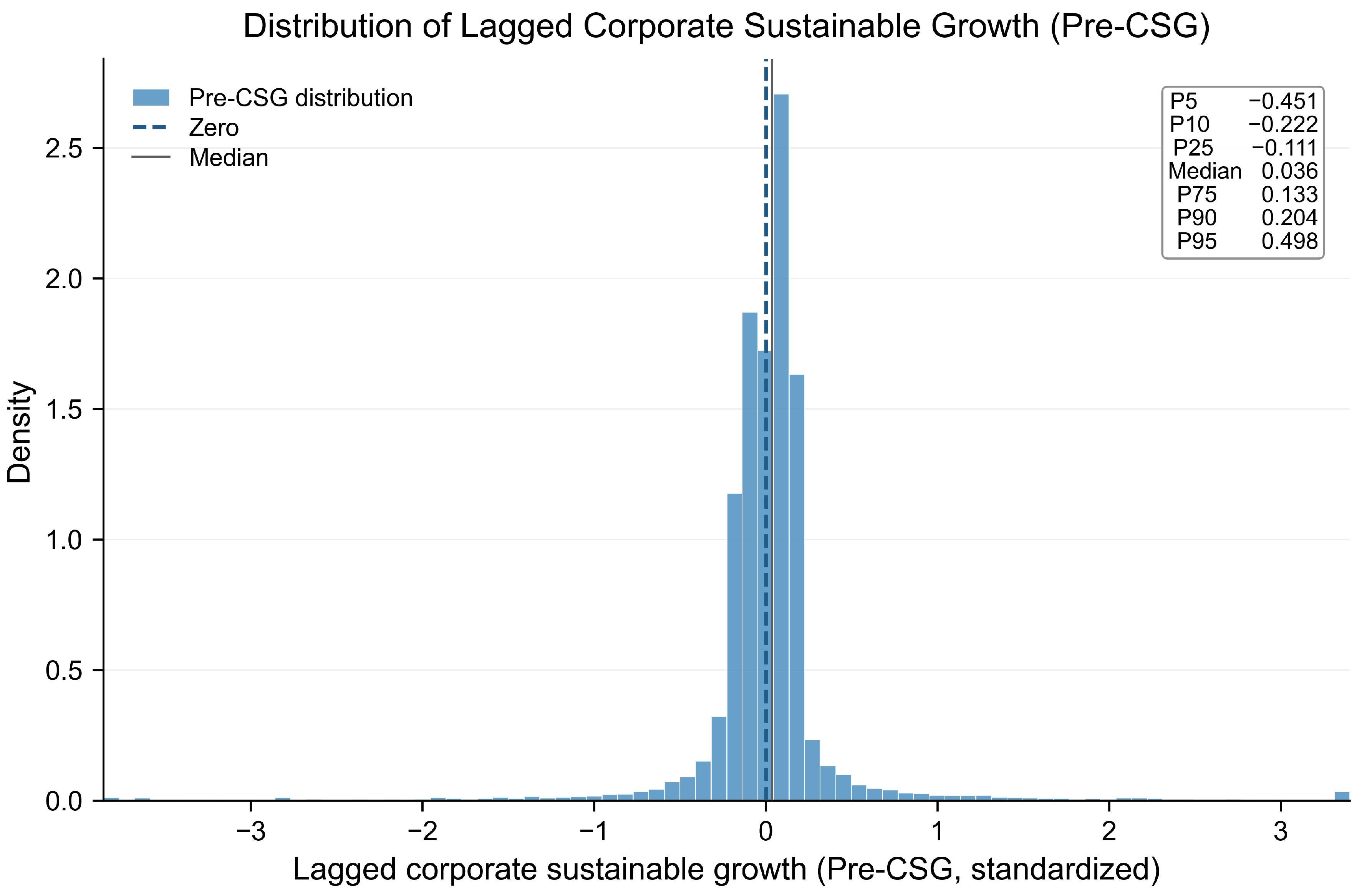
Table A2.
Pearson correlation matrix.
Appendix B. Construction of Corporate Sustainable Growth
Table A3.
Construction of corporate sustainable growth (CSG).
Appendix C. CFMSI Construction and Commodity Futures Universe
Table A4.
CFMSI construction and eligibility rules.
Table A5.
Commodity futures universe and entry into the CFMSI.
Table A6.
CFMSI dimension correlations, alternative-construction diagnostics, and leave-one-dimension-out results.
Table A7.
Leave-one-commodity-sector-out CFMSI results.
Table A8.
Directional commodity-price movement tests.
Table A9.
Sample construction and reproducibility workflow.
Table A10.
Additional Pre-CSG sensitivity tests.
References
- Garbade, K.D.; Silber, W.L. Price Movements and Price Discovery in Futures and Cash Markets. Rev. Econ. Stat. 1983, 65, 289–297. [Google Scholar] [CrossRef] [Scilit]
- Cheng, I.H.; Xiong, W. Financialization of Commodity Markets. Annu. Rev. Financ. Econ. 2014, 6, 419–441. [Google Scholar] [CrossRef] [Scilit]
- Ho, S.W.; Lauwers, A.R. Is There Smart Money? How Information in the Commodity Futures Market Is Priced into the Cross Section of Stock Returns with Delay. J. Financ. Quant. Anal. 2023, 58, 3201–3230. [Google Scholar] [CrossRef] [Scilit]
- Akyildirim, E.; Corbet, S.; Ryan, M.; Mukherjee, A. The Influence of Maritime Freight Cost Tail Risk on Publicly Traded Industrial and Transport Companies. J. Int. Money Financ. 2025, 157, 103358. [Google Scholar] [CrossRef] [Scilit]
- Mena, S.; Parker, S. The Temporal Structuring of Corporate Sustainability. J. Bus. Ethics 2024, 195, 1–23. [Google Scholar] [CrossRef] [Scilit]
- Berg, F.; Kölbel, J.F.; Rigobon, R. Aggregate Confusion: The Divergence of ESG Ratings. Rev. Financ. 2022, 26, 1315–1344. [Google Scholar] [CrossRef] [Scilit]
- Christensen, D.M.; Serafeim, G.; Sikochi, A. Why Is Corporate Virtue in the Eye of the Beholder? The Case of ESG Ratings. Account. Rev. 2022, 97, 147–175. [Google Scholar] [CrossRef] [Scilit]
- Avramov, D.; Cheng, S.; Lioui, A.; Tarelli, A. Sustainable Investing with ESG Rating Uncertainty. J. Financ. Econ. 2022, 145, 642–664. [Google Scholar] [CrossRef] [Scilit]
- Chava, S.; Kim, J.H.; Lee, J. Risk, Return, and Environmental and Social Ratings. J. Corp. Financ. 2025, 92, 102744. [Google Scholar] [CrossRef] [Scilit]
- Hoepner, A.G.F.; Oikonomou, I.; Sautner, Z.; Starks, L.T.; Zhou, X.Y. ESG Shareholder Engagement and Downside Risk. Rev. Financ. 2024, 28, 483–510. [Google Scholar] [CrossRef] [Scilit]
- Goodell, J.W.; Corbet, S.; Hou, Y.; Hu, Y.; Oxley, L. Isolating Defensive Corporate ESG Effects: Evidence from Purely Domestic Anti-COVID-19 Measures. J. Financ. Stab. 2024, 71, 101220. [Google Scholar] [CrossRef] [Scilit]
- Walker, T.; Fernandes, A.; Karami, M. Corporate Resilience during Crises and the Role of ESG Factors: Evidence from the COVID-19 Pandemic. Financ. Res. Lett. 2024, 69, 106168. [Google Scholar] [CrossRef] [Scilit]
- Liu, H.; Fan, W.; Li, C. From ESG Performance to Corporate Resilience: Evidence from China’s Manufacturing Industry. Sustainability 2025, 17, 9672. [Google Scholar] [CrossRef] [Scilit]
- Xing, Z.; Xie, Z. The Impact of ESG Performance on the Financial Resilience of Manufacturing Enterprises. Sustainability 2026, 18, 5634. [Google Scholar] [CrossRef] [Scilit]
- Yang, J.; Wang, J.; Wang, J. ESG Performance, Innovation Capability and Organizational Resilience Under Environmental Uncertainty: Evidence from China. Sustainability 2026, 18, 2806. [Google Scholar] [CrossRef] [Scilit]
- Yuan, Y.; Dai, H.; Ma, J. The Impact of Corporate ESG Performance on Supply Chain Resilience: A Mediation Analysis Based on New Quality Productive Forces. Sustainability 2025, 17, 4418. [Google Scholar] [CrossRef] [Scilit]
- Chang, Y.C.; Hsiao, P.J.; Ljungqvist, A.; Tseng, K. Testing Disagreement Models. J. Financ. 2022, 77, 2239–2285. [Google Scholar] [CrossRef] [Scilit]
- Liu, X.; Dai, J.; Dong, X.; Liu, J. ESG Rating Disagreement and Analyst Forecast Quality. Int. Rev. Financ. Anal. 2024, 95, 103446. [Google Scholar] [CrossRef] [Scilit]
- Derrien, F.; Krüger, P.; Landier, A.; Yao, T. ESG News, Future Cash Flows, and Firm Value. J. Financ. 2025, 80, 3499–3554. [Google Scholar] [CrossRef] [Scilit]
- Arif, S.; Golshan, N.M. The Value of Values: Does Focusing on Sustainability Provide a Competitive Advantage in Forecasting Earnings? Contemp. Account. Res. 2026, 43, 779–816. [Google Scholar] [CrossRef] [Scilit]
- Tang, K.; Xiong, W. Index Investment and the Financialization of Commodities. Financ. Anal. J. 2012, 68, 54–74. [Google Scholar] [CrossRef] [Scilit]
- Silvennoinen, A.; Thorp, S. Financialization, Crisis and Commodity Correlation Dynamics. J. Int. Financ. Mark. Inst. Money 2013, 24, 42–65. [Google Scholar] [CrossRef] [Scilit]
- Creti, A.; Joëts, M.; Mignon, V. On the Links between Stock and Commodity Markets’ Volatility. Energy Econ. 2013, 37, 16–28. [Google Scholar] [CrossRef] [Scilit]
- Ready, R.C. Oil Prices and the Stock Market. Rev. Financ. 2018, 22, 155–176. [Google Scholar] [CrossRef] [Scilit]
- Bakas, D.; Triantafyllou, A. Commodity Price Volatility and the Economic Uncertainty of Pandemics. Econ. Lett. 2020, 193, 109283. [Google Scholar] [CrossRef] [Scilit]
- Phan, D.H.B.; Tran, V.T.; Nguyen, D.T. Crude Oil Price Uncertainty and Corporate Investment: New Global Evidence. Energy Econ. 2019, 77, 54–65. [Google Scholar] [CrossRef] [Scilit]
- Caporale, G.M.; Menla Ali, F.; Spagnolo, N. Oil Price Uncertainty and Sectoral Stock Returns in China: A Time-Varying Approach. China Econ. Rev. 2015, 34, 311–321. [Google Scholar] [CrossRef] [Scilit]
- Luo, X.; Qin, S. Oil Price Uncertainty and Chinese Stock Returns: New Evidence from the Oil Volatility Index. Financ. Res. Lett. 2017, 20, 29–34. [Google Scholar] [CrossRef] [Scilit]
- Xiao, J.; Chen, X.; Li, Y.; Wen, F. Oil Price Uncertainty and Stock Price Crash Risk: Evidence from China. Energy Econ. 2022, 112, 106118. [Google Scholar] [CrossRef] [Scilit]
- Lins, K.V.; Servaes, H.; Tamayo, A. Social Capital, Trust, and Firm Performance: The Value of Corporate Social Responsibility during the Financial Crisis. J. Financ. 2017, 72, 1785–1824. [Google Scholar] [CrossRef] [Scilit]
- Albuquerque, R.; Koskinen, Y.; Yang, S.; Zhang, C. Resiliency of Environmental and Social Stocks: An Analysis of the Exogenous COVID-19 Market Crash. Rev. Corp. Financ. Stud. 2020, 9, 593–621. [Google Scholar] [CrossRef] [Scilit] [PubMed]
- Ding, W.; Levine, R.; Lin, C.; Xie, W. Corporate Immunity to the COVID-19 Pandemic. J. Financ. Econ. 2021, 141, 802–830. [Google Scholar] [CrossRef] [Scilit] [PubMed]
- Liu, D.; Gu, K.; Hu, W. ESG Performance and Stock Idiosyncratic Volatility. Financ. Res. Lett. 2023, 58, 104393. [Google Scholar] [CrossRef] [Scilit]
- Luo, W.; Tian, Z.; Fang, X.; Deng, M. Can Good ESG Performance Reduce Stock Price Crash Risk? Evidence from Chinese Listed Companies. Corp. Soc. Responsib. Environ. Manag. 2024, 31, 1469–1492. [Google Scholar] [CrossRef] [Scilit]
- Xu, Z.; Liu, D.; Li, Y.; Guo, F. ESG and Stock Price Volatility Risk: Evidence from Chinese A-share Market. N. Am. J. Econ. Financ. 2025, 75, 102277. [Google Scholar] [CrossRef] [Scilit]
- Eccles, R.G.; Ioannou, I.; Serafeim, G. The Impact of Corporate Sustainability on Organizational Processes and Performance. Manag. Sci. 2014, 60, 2835–2857, Erratum in Manag. Sci. 2025, 71, 3634. [Google Scholar] [CrossRef] [Scilit]
- Pástor, Ľ.; Stambaugh, R.F.; Taylor, L.A. Sustainable Investing in Equilibrium. J. Financ. Econ. 2021, 142, 550–571. [Google Scholar] [CrossRef] [Scilit]
- Pedersen, L.H.; Fitzgibbons, S.; Pomorski, L. Responsible Investing: The ESG-Efficient Frontier. J. Financ. Econ. 2021, 142, 572–597. [Google Scholar] [CrossRef] [Scilit]
- Bolton, P.; Kacperczyk, M. Do Investors Care about Carbon Risk? J. Financ. Econ. 2021, 142, 517–549. [Google Scholar] [CrossRef] [Scilit]
- Ilhan, E.; Sautner, Z.; Vilkov, G. Carbon Tail Risk. Rev. Financ. Stud. 2021, 34, 1540–1571. [Google Scholar] [CrossRef] [Scilit]
- Pástor, Ľ.; Stambaugh, R.F.; Taylor, L.A. Dissecting Green Returns. J. Financ. Econ. 2022, 146, 403–424. [Google Scholar] [CrossRef] [Scilit]
- Faccini, R.; Matin, R.; Skiadopoulos, G. Dissecting Climate Risks: Are They Reflected in Stock Prices? J. Bank. Financ. 2023, 155, 106948. [Google Scholar] [CrossRef] [Scilit]
- Brown, W.O.; Gao, X.; Han, Y.; Huang, D.; Wang, F. Environmental Sustainability and Stock Returns. J. Financ. Mark. 2026, 79, 101006. [Google Scholar] [CrossRef] [Scilit]
- Khan, M.; Serafeim, G.; Yoon, A. Corporate Sustainability: First Evidence on Materiality. Account. Rev. 2016, 91, 1697–1724. [Google Scholar] [CrossRef] [Scilit]
- Barron, O.E.; Kim, O.; Lim, S.C.; Stevens, D.E. Using Analysts’ Forecasts to Measure Properties of Analysts’ Information Environment. Account. Rev. 1998, 73, 421–433. [Google Scholar] [CrossRef] [Scilit]
- Diether, K.B.; Malloy, C.J.; Scherbina, A. Differences of Opinion and the Cross Section of Stock Returns. J. Financ. 2002, 57, 2113–2141. [Google Scholar] [CrossRef] [Scilit]
- Hong, H.; Stein, J.C. Differences of Opinion, Short-Sales Constraints, and Market Crashes. Rev. Financ. Stud. 2003, 16, 487–525. [Google Scholar] [CrossRef] [Scilit]
- Loh, R.K.; Stulz, R.M. Is Sell-Side Research More Valuable in Bad Times? J. Financ. 2018, 73, 959–1013. [Google Scholar] [CrossRef] [Scilit]
- Zhang, X.; Xiao, J.; Zhang, Z. An Anatomy of Commodity Futures Returns in China. Pac.-Basin Financ. J. 2020, 62, 101366. [Google Scholar] [CrossRef] [Scilit]
- Li, C.; Wu, C.; Zhou, C. Forecasting Equity Returns: The Role of Commodity Futures along the Supply Chain. J. Futur. Mark. 2021, 41, 46–71. [Google Scholar] [CrossRef] [Scilit]
- Dai, X.; Dai, P.F.; Wang, Q.; Ouyang, Z.Y. The Impact of Energy-Exporting Countries’ EPUs on China’s Energy Futures Investors: Risk Preference, Investment Position and Investment Horizon. Res. Int. Bus. Financ. 2023, 64, 101806. [Google Scholar] [CrossRef] [Scilit]
- Fan, J.H.; Fernandez-Perez, A.; Indriawan, I.; Todorova, N. When Chinese Mania Meets Global Frenzy: Commodity Price Bubbles. J. Commod. Mark. 2024, 36, 100437. [Google Scholar] [CrossRef] [Scilit]
- Zhao, R.; Xiong, X.; Ma, J.; Zhang, Y.; Zhang, Y. Baidu News and the Return Volatility of Chinese Commodity Futures: Evidence for the Sequential Information Arrival Hypothesis. Financ. Innov. 2025, 11, 80. [Google Scholar] [CrossRef] [Scilit]
- Parkinson, M. The Extreme Value Method for Estimating the Variance of the Rate of Return. J. Bus. 1980, 53, 61–65. [Google Scholar] [CrossRef] [Scilit] [PubMed]
- Amihud, Y. Illiquidity and Stock Returns: Cross-Section and Time-Series Effects. J. Financ. Mark. 2002, 5, 31–56. [Google Scholar] [CrossRef] [Scilit]
- Fama, E.F.; French, K.R. A Five-Factor Asset Pricing Model. J. Financ. Econ. 2015, 116, 1–22. [Google Scholar] [CrossRef] [Scilit]
- Ang, A.; Hodrick, R.J.; Xing, Y.; Zhang, X. The Cross-Section of Volatility and Expected Returns. J. Financ. 2006, 61, 259–299. [Google Scholar] [CrossRef] [Scilit]
- Cameron, A.C.; Gelbach, J.B.; Miller, D.L. Robust Inference with Multiway Clustering. J. Bus. Econ. Stat. 2011, 29, 238–249. [Google Scholar] [CrossRef] [Scilit]
- Cameron, A.C.; Gelbach, J.B.; Miller, D.L. Bootstrap-Based Improvements for Inference with Clustered Errors. Rev. Econ. Stat. 2008, 90, 414–427. [Google Scholar] [CrossRef] [Scilit]
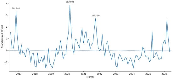
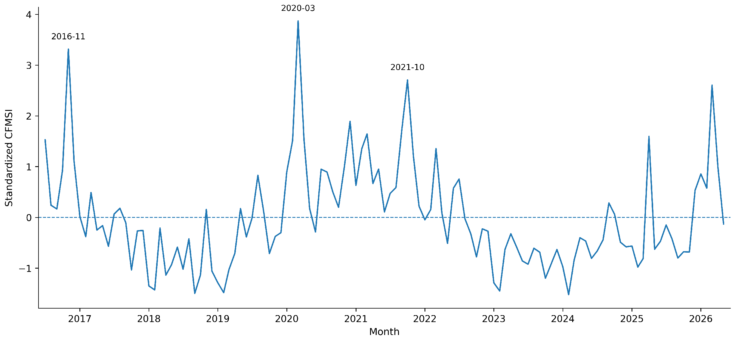
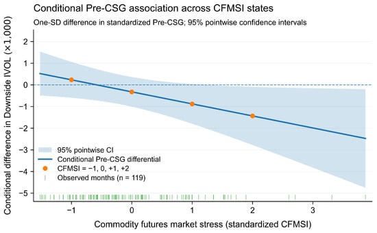
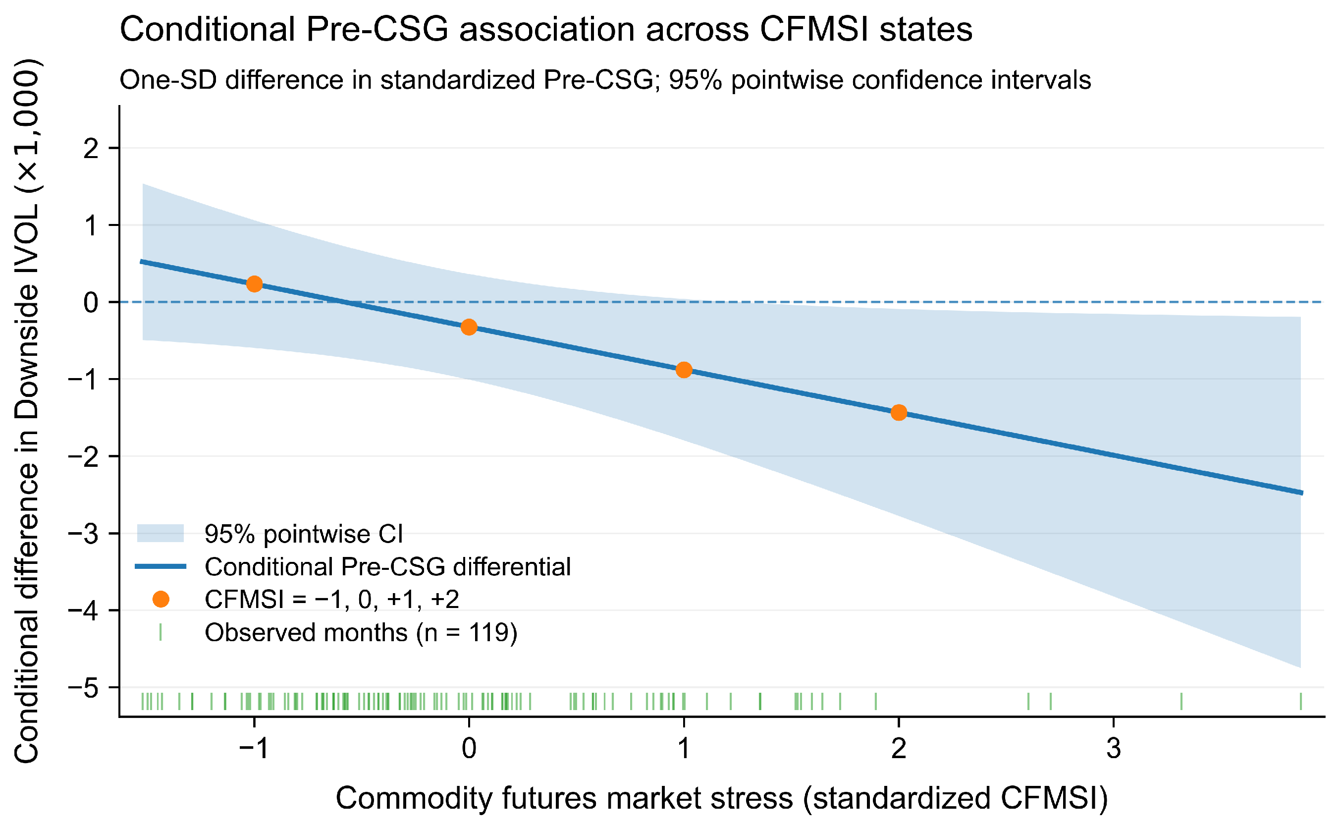

Disclaimer/Publisher’s Note: The statements, opinions and data contained in all publications are solely those of the individual author(s) and contributor(s) and not of MDPI and/or the editor(s). MDPI and/or the editor(s) disclaim responsibility for any injury to people or property resulting from any ideas, methods, instructions or products referred to in the content. |
© 2026 by the authors. Licensee MDPI, Basel, Switzerland. This article is an open access article distributed under the terms and conditions of the Creative Commons Attribution (CC BY) license.