


Abstract
Pork remains a cornerstone of many food systems, and fluctuations in its price are a critical concern for the economic sustainability of agricultural supply chains. This study connects epidemic associations, reserve-operation case studies and forecasting to examine pork price fluctuations in China using average retail prices in 36 major cities. Linear and nonlinear regressions examine epidemic conditions, while reserve cases compare price changes and pig-to-grain ratios. Chronological out-of-sample forecasts compare seven models at one-, three- and six-week horizons, with ordinary least squares as the principal benchmark. Direct-price and cumulative-change approaches are evaluated on the original price scale. The epidemic index exhibits a nonlinear association in the five-knot specification with year controls despite limited linear explanatory power. Reserve episodes show differing adjustment paths, and higher pig-to-grain ratios are not consistently accompanied by lower dispersion. Univariate autoregressive integrated moving average (ARIMA) achieves the lowest root mean squared error in most comparisons, while market indicators improve selected forecasts. Support vector regression using price history and slaughter profits under the cumulative-change approach yields the lowest three-week errors among the evaluated main-sample configurations. These findings inform market monitoring and the selection of forecasting indicators and models.
1. Introduction
The pork industry plays a vital role in national economies, contributing to employment and agricultural supply chains [1]. Beyond its economic footprint, the stability of pork prices is linked to the socio-economic sustainability of food markets [2], particularly in countries where pork is a staple. Severe price fluctuations affect household food expenditures and the economic viability of producers [3,4]. Rising prices can encourage substitution toward other meats, while steep price declines erode producers’ revenues, and may place small-scale farmers under financial pressure [5].
In China, these dynamics manifest in the well-known “pork cycle”—periodic fluctuations in supply and price driven by production lags and market expectations [6]. The cyclical alternation of oversupply and shortage intensifies price volatility and challenges the long-term economic stability of the sector. Consequently, understanding and monitoring these fluctuations is important for market resilience. China employs policy instruments [7,8], including reserve purchases and releases, to absorb market shocks and stabilize prices [5].
Theoretical and empirical research has long examined the determinants of pork price cycles [9]. Early work by Coase and Fowler [10] analyzed the pig cycle in Great Britain, while Ezekiel [11] examined price fluctuations arising from lagged supply responses. Harlow [12] extended this framework, identifying a roughly four-year pork price cycle in the historical U.S. setting and relating it to endogenous industry dynamics. Subsequent studies explored how information lags and farmer behavior amplify or dampen cycles; Hayes and Schmitz [13] highlighted counter-cyclical adjustments by informed farmers. In the U.S., Parcell [14] documented seasonality in wholesale pork prices and demand.
More recently, scholarship has shifted toward forecasting methods to support sustainable decision-making by producers, traders, and policymakers [15,16]. Yang and Zhang [17] developed a data-driven causal network framework for examining pork price dynamics in Sichuan Province. Lin et al. [18] proposed VMD–EMSA–HCTM–Informer, a hybrid univariate framework for forecasting pork prices. Ma et al. [19] combined forecasts from 11 econometric and machine learning methods using six combination strategies to forecast hog prices and design production plans. Integrated approaches, such as that by Guo et al. [20], who combined AttLSTM, ARIMA, and BP neural networks for corn price forecasting, illustrate the use of hybrid models in agricultural markets. Further refinements by Guo et al. [21] incorporated an STL–FA–AttGRU model for hog prices, and they reported lower errors in their model comparison. A comprehensive review [22] highlights both the breadth of techniques—including neural networks, time-series models, and hybrids—and challenges in their evaluation. This literature motivates comparing predictive information and forecasting methods under a common evaluation design [23].
On the supply side, feed costs represent a major share of pig farming expenses, linking grain prices to production costs [24]. On the demand side, income growth and consumer preferences [25,26] shape demand for livestock-derived foods [27]. External shocks such as epidemics and supply chain disruptions further contribute to price instability, posing challenges to the resilience and economic sustainability of the sector [3,5,28]. Economic policy and industry news uncertainty can also affect prices along the pig industry chain [29]. These conditions make disease indicators, producer price–cost conditions and market information [30,31] relevant to the interpretation and monitoring of pork price movements.
While existing studies have examined price cycles, epidemic effects and forecasting methods, practical market monitoring requires connecting the interpretation of observed fluctuations with the assessment of future prices. Using the Average Retail Pork Price in 36 Major Cities (ARP-36), this study examines three related questions: whether the association between epidemic conditions and retail prices is adequately represented by a linear relationship; how price changes and producer price–cost conditions evolve around selected storage and release events; and whether feed prices and slaughter profits add predictive information beyond price history. The forecasting comparison also assesses whether nonlinear models improve on OLS. Together, these questions link the analysis of market conditions and observed adjustments with the evaluation of price forecasts.
This study makes three contributions. First, it compares linear and nonlinear associations between the porcine epidemic index and retail pork prices, using natural cubic splines with year controls to examine variation beyond a constant slope. Second, it examines selected storage and release episodes using a common price-change measure, complemented by comparisons of pig-to-grain ratio levels and dispersion. The comparisons distinguish changes in relative price levels from changes in their dispersion. Third, it evaluates the incremental predictive information in feed prices and slaughter profits through chronological out-of-sample comparisons, using OLS as the principal benchmark alongside ARIMA, VAR, a naive forecast, and Machine Learning and Deep Learning models. Parallel direct price and cumulative change approaches are evaluated on the original price scale at one-, three- and six-week horizons. The comparison separates gains from additional indicators from gains associated with model choice.
The findings reveal a nonlinear epidemic–price association within the five-knot specification with year controls and differing paths of adjustment around the selected reserve episodes. Price history remains a competitive forecasting baseline: the univariate ARIMA benchmark achieves the lowest RMSE in most comparisons with models using either price history alone or price history augmented by both market indicators. SVR incorporating slaughter profit information under the cumulative change approach achieves the lowest three-week errors among the evaluated main-sample configurations. These findings support assessing market indicators and forecasting methods in relation to the conditions and horizons for which they are used.
The remainder of the paper is structured as follows. Section 2 describes the data sources and methodology. Section 3 presents the empirical results, encompassing epidemic associations, reserve operation case studies, and comparative price forecasting. Section 4 provides a detailed discussion and Section 5 contains concluding remarks and policy implications.
2. Data and Methodology
2.1. Data
The primary dataset for this study is obtained from the iFind Database, supplemented with publicly available information from the National Development and Reform Commission, the National Bureau of Statistics, and Yongyi Consulting. The dataset includes daily and weekly price data, covering 14 indexes. These include the average retail price of pork in 36 major cities, observed pork import and export quantities, designated slaughter volumes of live pigs, weekly pig feed prices, weekly slaughter profits, the pig–grain ratio, average prices and quantities of storage release, and disease indices, among others. Weekly data are prioritized for predictive modeling to align price observations with the weekly feed price and slaughter profit indicators. Sample coverage differs across the analyses and is reported with the corresponding results.
The 36 cities are Beijing, Tianjin, Shijiazhuang, Taiyuan, Hohhot, Shenyang, Dalian, Changchun, Harbin, Shanghai, Nanjing, Hangzhou, Ningbo, Hefei, Fuzhou, Xiamen, Nanchang, Jinan, Qingdao, Zhengzhou, Wuhan, Changsha, Guangzhou, Shenzhen, Nanning, Haikou, Chongqing, Chengdu, Guiyang, Kunming, Lhasa, Xi’an, Lanzhou, Xining, Yinchuan, and Urumqi. The study uses the aggregate retail pork price series officially published by the National Development and Reform Commission (NDRC).
In addition, five supplementary data sources are consulted: Akshare, Wind, the Bric Rural Agriculture Database, the Ministry of Agriculture and Rural Affairs, and Zhuochuang Information (Pork Industry). These multiple sources provide a comprehensive dataset for empirical analysis.
2.2. Methodology
2.2.1. Data Processing
An initial pool of 35 potential explanatory factors was compiled, including key economic and production indicators such as the break-even point, pig–grain ratio, farm scale, CR5 concentration ratio, per capita pork consumption, the number of small farms, the Consumer Price Index (CPI), the Producer Price Index (PPI), weaning and parturition rates, and costs associated with feed, vaccines, and labor.
The dependent variable is defined as the Average Retail Pork Price in 36 Major Cities (ARP-36). Independent variables are drawn from the broader dataset, with the indicators used in each analysis specified below.
For forecasting, data are aligned to Fridays. ARP-36 takes the last actual quotation within each week, while each predictor takes its latest recorded value available by that Friday. Predictor values may be carried forward; missing ARP-36 quotations are not filled. The common long sample runs from 6 January 2017 to 19 August 2022, comprising 294 calendar weeks and 292 observed weekly prices. The full weekly calendar is retained when constructing histories and forecast targets.
Stationarity is assessed using the Augmented Dickey–Fuller (ADF) and Kwiatkowski–Phillips–Schmidt–Shin (KPSS) tests on levels and first differences. Both include a constant without a deterministic time trend; ADF lags are selected by the Akaike information criterion and KPSS uses automatic bandwidth selection. The daily price diagnostics and the initial weekly forecasting sample diagnostics are conducted separately, as they concern different frequencies and estimation periods.
2.2.2. Epidemic Association Analysis
The Local Outlier Factor (LOF) algorithm identifies unusual price observations by comparing their local densities with those of neighboring observations. The epidemic analysis then uses 44 matched monthly observations from July 2018 to August 2022, with the monthly mean ARP-36 as the main price measure. A univariate ordinary least squares (OLS) regression is followed by logarithmic, exponential, power and quadratic-to-quartic polynomial specifications. Natural cubic splines accommodate local variation in the price–index association. The five-knot specification uses the 5th, 27.5th, 50th, 72.5th and 95th percentiles of the observed index and includes year fixed effects.
where pm is the monthly mean ARP-36 and Im is the epidemic index for month m. In Equation (1), α is the intercept, β is the linear slope and εm is the residual. Equation (2) adds three nonlinear spline basis functions Bj(Im), with coefficients γj, and year fixed effects δy(m), with one reference year omitted; y(m) identifies the year containing month m. The last observed monthly quotation replaces the mean in the corresponding sensitivity analysis.
pm = α + βIm + εm
Joint tests distinguish overall association from nonlinearity using HAC(3), measured over actual calendar months, and HC3 covariance estimates. Holm adjustment covers the ten examined nonlinear price-level specifications. Sensitivity analyses vary spline flexibility, the monthly price measure, within-year trends, sample composition and lagged-price controls. Sample exclusions retain the full-sample knot locations. Exploratory extensions relate six-month cumulative log price changes to the index change and its square, and subsequent three-month volatility to the absolute index change. Additional specifications include prior price controls and seasonal terms or year fixed effects; HAC(6) is also considered for overlapping six-month outcomes and used for subsequent volatility.
The subsequent three-month volatility measure is defined as
where rm is the monthly log change in ARP-36, expressed as a percentage, and Vm,3 is the root mean square of these changes over the three calendar months following month m.
2.2.3. Storage and Release Operation Case Studies
Seasonal Trend Decomposition using Loess (STL) is applied to decompose ARP-36 into trend, seasonal, and residual components [32,33]. The reserve operation case studies examine a storage operation on 21 July 2021 and a release operation on 15 January 2021 over one-, three-, and six-month windows. Price movements are measured using first differences between consecutive available price observations. Local maxima and minima are identified using SciPy’s peak detection algorithm, and the calendar intervals between each intervention and the subsequent observed extrema are used to characterize the timing of price movements.
For the broader analysis of storage operations, the timing measure is defined as the calendar interval between each storage operation and the maximum first difference observed within the corresponding one-, three-, or six-month window. The analysis includes only operations with positive recorded procurement volumes and complete observation windows. Both window endpoints are included, and when the maximum first difference occurs on multiple dates, the earliest occurrence is used.
For each case, an OLS regression of price changes on a constant and a post-intervention indicator compares the one-month pre- and post-intervention means. The event date belongs to the post-intervention window.
where qi is an observed ARP-36 quotation, i indexes consecutive available observations, and Δqi = qi − qi−1 is their price change. Within the selected one-month windows, Posti equals 0 before the operation and 1 on or after its date. The intercept α is the pre-operation mean change, θ is the post-minus-pre mean difference, and ui is the residual. Inference uses Newey–West HAC standard errors with three lags of consecutive available observations and Holm adjustment across the two cases. Complementary pig-to-grain comparisons retain ratio levels, and calculate means and standard deviations from available weekly observations within 30 calendar days before and after each event, excluding the event date and without interpolation. These case comparisons describe observed selected episodes.
Δqi = α + θPosti + ui
2.2.4. Model Training and Forecasting
To evaluate predictive performance, OLS is employed as the principal benchmark for training and forecasting, alongside Support Vector Regression (SVR), Extreme Gradient Boosting (XGBoost), and Long Short-Term Memory (LSTM) models. Four information sets contain price history alone, price history with the Weekly Price of Pig Feed (WPF), price history with the Weekly Gross Profit of Live Pig Slaughter (WGP-LS), and price history with both indicators. These four models use the current and preceding three weeks of the selected inputs, with separate direct models for each horizon.
Two parallel approaches compare forecasting representations. For the four supervised models, Approach A uses input levels to predict future prices directly:
Approach B uses first-differenced inputs to predict the cumulative price change directly, and then reconstructs the future price,
where Pt is ARP-36 at weekly forecast origin t and h is the forecast horizon of one, three or six calendar weeks. The input vector contains the current and preceding three weeks of the selected level series; contains their first differences. The fitted functions and target the future price and the cumulative change Zt,h, respectively, with ΔPt = Pt − Pt−1. Thus, Approach B predicts one horizon-specific cumulative change, while both approaches yield forecasts on the original price scale.
Zt,h = Pt+h − Pt
Autoregressive Integrated Moving Average (ARIMA) provides a univariate benchmark, fitting price levels in Approach A and first differences in Approach B. Vector Autoregression (VAR) jointly models the first differences of the multivariate information sets and accumulates predicted price changes. ARIMA and VAR forecast recursively. A naive forecast carries forward the latest observed price; VAR and naive forecasts are shared across approaches.
SVR uses a radial basis function kernel, XGBoost uses regression trees with a squared-error objective, and LSTM uses one recurrent layer with 8 or 16 hidden units and a linear output, trained with Adam. SVR (version 1.8.0) and LSTM standardize inputs and targets using only the applicable training data. Appendix A reports fixed configurations, search spaces and selected hyperparameters.
2.2.5. Forecast Horizons and Hyperparameter Selection
To examine how accuracy varies with forecast horizon, the study constructs forecasts with step sizes of 1, 3 and 6 calendar weeks ahead. The initial training period contains 156 calendar weeks, ending on 27 December 2019. The estimation window subsequently expands by one week, and models are re-estimated at each eligible weekly forecast origin.
Hyperparameters are selected once within the initial training period using Optuna’s tree-structured Parzen estimator (TPE), with 50 attempted trials for each tunable model configuration and horizon, and seed 42. Three expanding validation folds (TSCV) each contain 13 calendar weeks of forecast origins; all validation targets are observed by the initial training cutoff. Each block approximates a quarter while retaining over two years of preceding training history. Models are fitted once at each fold’s starting origin; subsequent predictions use then-available inputs, and ARIMA updates its filtered state without parameter re-estimation. Hyperparameter selection minimizes the arithmetic mean of the three validation RMSEs,
where λ denotes the hyperparameters of a given model, information set, approach and horizon, and Λ contains the successfully evaluated trial configurations. RMSEk,h is the price-scale RMSE in validation fold k, after inverse scaling and price reconstruction where applicable. The selected configuration remains fixed out of sample, while model parameters and applicable scalers are re-estimated weekly. OLS and the naive forecast have fixed specifications.
The Daily Price Spread for Standard and Fat Hogs (DPS) is examined separately over its shorter common sample, using 52 initial training weeks and three validation folds of six weeks each. Both information sets include price history, WPF and WGP-LS, with DPS added to the augmented set. Hyperparameters are tuned within this training sample.
2.2.6. Forecast Comparison
Finally, the study compares predicted pork prices with actual observations across time horizons. Model performance is evaluated using Root Mean Square Error (RMSE), Mean Squared Error (MSE) and Mean Absolute Percentage Error (MAPE), with Mean Absolute Error (MAE) also reported for selected comparisons. All metrics use inverse-scaled, reconstructed price forecasts where applicable. We define the forecast error as . The evaluation measures are
where is the common set of eligible out-of-sample forecast origins for horizon h, Nh = || is its size, Pt+h is the observed positive future ARP-36 price, and is the corresponding price forecast. In the main sample, models, information sets and approaches share the same evaluation dates within each horizon, with Nh equal to 126, 124 and 122 at one, three and six weeks, respectively. RMSE and MAE are in price units, MSE is in squared price units, and MAPE is a percentage with observed prices as its denominator.
Percentage RMSE reductions are calculated from unrounded errors,
where C denotes the candidate forecast and R the reference forecast. OLS is the principal reference for model comparisons, which hold the information set and approach fixed; information-addition comparisons hold the model and approach fixed and use price history alone as the reference. A positive reduction indicates a lower RMSE than the stated reference. Selected comparisons of paired squared forecast losses use calendar-based Newey–West HAC tests and paired block resampling.
By combining epidemic association analysis, reserve-operation case studies and comparative forecasting, this methodology provides an empirical foundation for the subsequent analysis and discussion presented in Section 3.
3. Results
3.1. Pork Price Anomalies and Epidemic Associations
3.1.1. Anomaly Analysis and Disease Single-Factor Test
This study employs a machine learning-based anomaly detection method, specifically the density-based Local Outlier Factor (LOF) algorithm, to examine pork price fluctuations between 2014 and 2023. The analysis identifies unusual price observations and their timing within the sample.
The results show substantial pork price fluctuations during 2019–2022, a period that included African swine fever outbreaks and supply-chain disruptions [5]. Price fluctuations during this period were greater than in other years, underscoring the extent of supply–demand disequilibrium. The chosen timeframe provides both a long-term perspective on price trends and coverage of recent epidemic-related shocks affecting global markets.
Figure 1 presents the anomaly analysis, where the blue data points highlight periods of significant price fluctuations detected by the machine learning algorithm.
Figure 1.
Price anomaly analysis. LOF is an unsupervised anomaly detection algorithm based on “local density”. It determines whether a point is an outlier by comparing the density difference between a point and its neighbors. Let parameter k (number of neighbors) be used. For each point p, calculate the distance from it to all other points. Determine the distance to the kth closest point, called k − distance(p). The second step is to calculate the reachability distance. For each neighbor o of p, define reach − distk(p,o) = max{k − distance(o),d(p,o)}, where d(p,o) represents the Euclidean distance between p and o. The third step is to calculate the local reachability density (LRD), , where |Nk(p)| is the number of neighbors within the k-distance neighborhood. Step 4: Calculate the local outlier factor (LOF). , which is the average density of neighbors over the local density. Finally, determine whether the value is outlier based on the LOF value. An LOF of approximately 1 indicates a normal value; LOF > 1 indicates an outlier; LOF < 1 indicates a cluster center value. Blue dots indicate observations identified as outliers by the LOF algorithm, whereas red dots indicate observations not identified as outliers.
These results identify periods of unusual pork price movements from 2019 to 2022, providing a basis for the subsequent analysis of epidemic–price associations.
3.1.2. Associations Between the Porcine Epidemic Index and Pork Prices
To further test the role of epidemic shocks, this study examines the association of porcine epidemic disease index. The index quantifies the scope and severity of pig disease outbreaks, incorporating frequency, geographic spread, and impacts on the pig population, with data sourced from the iFind database. A univariate OLS regression of the ARP-36 on the porcine epidemic index from July 2018 to August 2022 yields an adjusted R2 of 0.0143 and an insignificant index coefficient (p = 0.210; HAC (3), p = 0.417). The weak linear fit motivates an examination of nonlinear associations. Logarithmic, exponential and power specifications yield R2 values of 0.0430, 0.0313 and 0.0364, respectively, indicating similarly limited explanatory power. Polynomial specifications provide a closer fit, with R2 values of 0.1633, 0.2489 and 0.3165 for the quadratic, cubic and quartic models. The quartic model also exhibits significant curvature in the absence of year controls (HAC (3), p = 0.00923).
The quartic curvature test becomes insignificant after year fixed effects are included (HAC(3), p = 0.3901). The highest-degree terms have HAC(3) p = 0.0706 for cubic versus quadratic and p = 0.1346 for quartic versus cubic, providing certain evidence that progressively higher orders may be suggested.
The balance between supply disruptions and demand responses may vary across epidemic conditions, suggesting that a constant slope may be a restrictive description of the price–index association. A natural cubic spline accommodates such local variation through smoothly joined cubic segments with linear tails. The five-knot specification uses the 5th, 27.5th, 50th, 72.5th and 95th percentiles of the observed index. Year fixed effects allow average price levels to differ across years.
In the five-knot specification, the results provide evidence of a nonlinear association between the recorded index and monthly retail prices. The five-knot model has R2 = 0.7603 and adjusted R2 = 0.7055 (Table 1, column 1). After controlling for year effects, the joint tests suggest an overall statistical association with the ARP-36 (Table 1, rows 3 and 4). The three nonlinear spline terms are jointly significant under both HAC (3) (p = 0.00162) and HC3 (p = 0.00518). The HAC (3) curvature test remains statistically significant after Holm adjustment across the ten examined nonlinear price-level specifications (p = 0.0162). Within this specification, the fitted curve is nonmonotonic and has an estimated local trough near an index value of 1.08. This fitted pattern suggests that the estimated association may vary across the observed index range, a feature that is not represented by a single linear coefficient.
Table 1.
Five-knot natural cubic spline estimates under alternative price measures and time controls.
Within the five-knot specification, evidence of curvature is also observed under two alternative specifications. Using the last available daily quotation within each month continues to yield statistically significant curvature tests under both covariance estimators (Table 1, column 2). This serves as a sensitivity check on whether averaging daily prices within each month accounts for the result; month-end observations also have precedent in research [34]. Allowing each year to have its own linear price trend also yields statistically significant curvature tests (column 3). These results suggest that the estimated curvature is not eliminated by controlling for differences in average prices or linear price movements within years.
The estimated pattern nevertheless depends on spline flexibility and sample composition. Three- and four-knot specifications with the same year controls do not exhibit significant curvature (HAC (3), p = 0.881 and 0.972, respectively). The five-knot specification captures local variation that is not detected by these less flexible alternatives. Excluding 2021 or the months with an index value of 1.08 retains marginal significance at the 10% level under HAC (3), although the corresponding HC3 tests are insignificant (Table 2). Adding the previous month’s price leaves the curvature significant under HAC (3), but not under HC3.
Table 2.
Sensitivity of the five-knot spline to sample composition and price persistence.
Exploratory extensions also provide evidence of possible nonlinear associations with subsequent price movements. Across 35 eligible starting months, the squared monthly index change is significant in a regression of six-month cumulative log price changes that also includes the linear index change (HAC (3), p = 0.0000124). The squared term continues to yield significance after controlling for the preceding three-month price trend and volatility (p = 0.00950); adding seasonal terms gives p = 0.0515, indicating significance at the 10% level. Replacing seasonal terms with year fixed effects gives p = 0.735.
For the following three months, volatility is measured by the root mean square of monthly log price changes expressed in percentage terms. Across 38 eligible starting months, the estimated coefficient indicates that a 0.1-unit increase in the absolute index change is associated with a 2.50-percentage-point lower volatility measure after controlling for prior price movements and seasonality (HAC (6), p = 0.000692). This association attenuates when year fixed effects replace seasonal controls.
Because the six-month outcomes overlap, inference is also examined with HAC(6). Corresponding p-values are 0.0000292 without additional controls, 0.0190 with prior price controls, 0.0779 with seasonal terms and 0.660 with year fixed effects. With year fixed effects, the coefficient is −0.105 percentage points and the HAC(6) p-value is 0.894.
Overall, the results provide evidence of a nonlinear association within the five-knot specification, while also showing sensitivity to spline flexibility, sample composition, and covariance estimation. The nonmonotonic fitted shape suggests that higher recorded index values are not uniformly associated with higher prices within this sample, and that a constant-slope model may provide an incomplete description of the observed relationship.
3.2. Time Lag of the Impact of Storage Behavior on Pig Prices
To analyze the temporal dynamics of pig prices, the study employs the Seasonal Trend Decomposition Procedure based on Loess (STL), a robust time series analytical technique capable of decomposing the series into trend, seasonal, and residual components [32,33]. The trend component reveals long-term price movements, seasonal components capture regular intra-annual patterns, and residuals reflect irregular or exogenous shocks [32]. STL’s flexibility enables it to accommodate evolving seasonal effects and preserve nonlinear data characteristics, making it indispensable for descriptive and forecasting purposes.
As shown in Figure 2, the STL decomposition of the pig price series from June 2015 to August 2022 reveals distinct trends, seasonal, and residual components. The trend component shows a pronounced increase around 2019–2020, followed by a decline towards 2022, indicating a period of substantial market adjustment. The seasonal component displays consistent intra-annual fluctuations, underscoring the strong role of seasonality in shaping pork price dynamics. The residual component captures irregular fluctuations after removing deterministic patterns and likely reflects short-term market shocks, abrupt shifts in supply and demand, or exogenous disturbances. Spikes in the residuals correspond to outlier events at specific points in time. Overall, the STL decomposition illustrates the trend and seasonal components of the price series. Its stationarity is examined separately using formal statistical tests.
Figure 2.
STL seasonal decomposition of pig prices. STL is a classic decomposition method in time series analysis. It breaks a time series into three components: trend, seasonality, and residual. A time series yt can be expressed as yt = Tt + St + Rt, where Tt is the trend term, representing the long-term direction of change; St is the seasonal term, reflecting cyclical fluctuations; and Rt is the residual term, representing random fluctuations or irregular noise. STL uses Loess smoothing (locally weighted regression) to estimate Tt and St. The decomposition plot clearly shows that pork prices exhibit both cyclical and trend patterns.
To prepare the series for the analysis of short-term price changes, first-order differencing is applied to address potential unit-root non-stationarity [33]. The first difference, defined in Section 2.2.3, measures the absolute price change between consecutive available observations. This transformation facilitates the description of price changes around the selected interventions.
The stationarity of the series is assessed using the Augmented Dickey–Fuller (ADF) test, complemented by the Kwiatkowski–Phillips–Schmidt–Shin (KPSS) test. The tests use the available ARP-36 series from 25 June 2015 to 24 August 2022, comprising 1774 price observations and 1773 first differences. Both tests include a constant but no deterministic time trend. ADF lag lengths are selected using the Akaike information criterion, yielding 24 lags for the level series and 23 for the differenced series. The KPSS test uses automatic bandwidth selection, yielding truncation lags of 27 and 25, respectively.
For the original pork retail price series from 36 major cities, the ADF test statistic is −1.724, which is greater than the critical values at the 1%, 5%, and 10% significance levels (−3.43, −2.86, and −2.57, respectively). The corresponding p-value of 0.419 indicates that the null hypothesis of a unit root cannot be rejected. By contrast, the ADF test on the first-order differenced series rejects the null hypothesis, with a test statistic of −6.061 and a p-value of 1.2145 × 10⁻⁷. The KPSS test rejects the null hypothesis of level stationarity for the original series (statistic = 1.673, p-value < 0.01) but does not reject it for the first-order differenced series (statistic = 0.149, p-value > 0.10). Together, these results support the use of first differences for the analysis of short-term price changes.
This section adopts a case-study approach to examine pork price dynamics following selected government storage and release interventions. Local peaks and troughs are identified in the plotted series within one-, three-, and six-month windows after the selected intervention dates. These time-stamped observations describe the timing and pattern of price movements over the different horizons where the interpretation is limited to the selected cases.
To further examine price dynamics following the selected government storage and release interventions, the analysis considers both price movements and recorded procurement and release volumes. Price movements describe the observed market trajectory, while the recorded volumes provide information on the scale of the selected operations. This two-dimensional perspective provides context for interpreting price patterns within the selected cases.
Specifically, storage operations are typically implemented when prices are low, aiming to support the market and counter downward price pressures. In contrast, release operations are generally implemented when prices are high, with the objective of stabilizing the market and curbing excessive price increases [5]. To examine short-term price movements on a consistent basis, the first-differenced price series is used for both storage and release cases. This series measures the absolute price change between consecutive available observations, allowing price movements following the selected interventions to be described using the same transformation.
Figure 3, Figure 4 and Figure 5 illustrate local peaks and troughs in the first-differenced ARP-36 series over one-, three-, and six-month windows following the storage operation on 21 July 2021. In these figures, red dots denote local maxima, while green dots denote local minima in price changes. These extrema describe local variation in the first-differenced series. Together, the figures provide a descriptive view of price movements over different observation windows within the selected storage case.
Figure 3.
Pork price changes over one month following the selected storage operation. This figure illustrates the first-differenced ARP-36 series over the one-month period following the storage operation on 21 July 2021. The blue line represents absolute price changes between consecutive available observations. Red and green dots denote local maxima and minima in the differenced series, respectively, identified using the SciPy peak detection algorithm.
Figure 4.
Pork price changes over three months following the selected storage operation. This figure extends the observation window to three months after the storage operation on 21 July 2021. The blue line represents the first-differenced ARP-36 series, with local maxima and minima marked in red and green, respectively. The extended window provides a broader view of the price changes observed following this event.
Figure 5.
Pork price changes over six months following the selected storage operation. This figure depicts the first-differenced ARP-36 series over the six-month period following the storage operation on 21 July 2021. The blue line shows changes between consecutive available price observations, while red and green dots identify local maxima and minima, respectively. These fluctuations describe the evolution of price changes within the selected six-month window.
The release case focuses on 15 January 2021, the earliest release date in 2021, placing both selected storage and release cases within the same calendar year. Figure 6, Figure 7 and Figure 8 illustrate local peaks and troughs in the first-differenced ARP-36 series over one-, three-, and six-month windows following this operation. Red dots denote local maxima, while green dots denote local minima in price changes. As subsequent reserve operations also occur within these windows, the figures are interpreted as descriptive evidence for the selected episode.
Figure 6.
Pork price changes over one month following the release operation on 15 January 2021. This figure illustrates the first-differenced ARP-36 series within the observation window from 15 January to 15 February 2021. The blue line represents absolute price changes between consecutive available observations. Red and green dots denote local maxima and minima, respectively.
Figure 7.
Pork price changes over three months following the release operation on 15 January 2021. This figure extends the observation window to 15 April 2021. The blue line represents the first-differenced ARP-36 series, with local maxima and minima marked in red and green, respectively. The extended window provides a broader view of the price changes observed during the selected episode.
Figure 8.
Pork price changes over six months following the release operation on 15 January 2021. This figure depicts the first-differenced ARP-36 series through 15 July 2021. The blue line shows changes between consecutive available price observations, while red and green dots identify local maxima and minima, respectively. These fluctuations describe the evolution of price changes within the selected six-month window.
An important metric for examining post-intervention price dynamics is the number of days between an intervention and an observed extreme in the price-change series within a specified window. This duration helps characterize the timing of subsequent price adjustments. In economic practice, storage and release interventions constitute key instruments for balancing supply and demand and stabilizing market prices [5]. Within the selected cases, the largest positive price change following the storage operation on 21 July 2021 occurred 21 days after the intervention in the one-month window and 96 days after the intervention in the six-month window. For the release operation on 15 January 2021, the largest negative price change occurred 13 and 87 days after the intervention in the corresponding windows. Thus, both cases exhibited price movements in the intended policy direction within the first month, while larger movements in that direction occurred in subsequent months. These observations highlight the value of considering both short-term fluctuations and later price developments when examining the selected storage and release episodes.
As illustrated in Figure 9, the timing of maximum price changes varies across storage operations and observation horizons. Within the available complete windows, the intervals range from 0 to 31 days for the one-month horizon, 28 to 90 days for the three-month horizon, and 96 to 110 days for the six-month horizon. These observations show that the most pronounced positive price changes occurred at different stages of the selected post-intervention periods.
Figure 9.
Time to maximum price changes following storage operations. The figure reports the calendar days between each storage operation and the maximum first difference of ARP-36 within one-month (blue), three-month (orange), and six-month (green) windows. Operations with positive recorded procurement volumes are included. Each window includes the intervention date and its corresponding end date; ties are resolved by selecting the earliest occurrence. Only complete windows are reported, yielding 16, 12, and 3 observations for the respective horizons. Smaller values indicate that the maximum price change occurred closer to the intervention date.
Within the selected storage cases, several operations share the same subsequent peak-change date. For the operations on 7, 14, and 21 July 2021, the maximum price change within the six-month window occurred on 25 October 2021, producing intervals of 110, 103, and 96 days, respectively. Similarly, the three-month maxima following the operations on 14 April, 29 April, 13 May, and 20 May 2022 all occurred on 6 July 2022. The corresponding intervals declined from 83 to 68, 54, and 47 days. This clustering indicates that multiple operations were followed by the same prominent market movement. The shorter intervals in these groups reflect intervention dates progressively closer to that shared peak.
To complement the timing analysis, an exploratory comparison of mean price changes is conducted over the one-month periods before and after each selected storage and release intervention. For each case, Equation (4) is estimated by OLS. The coefficient θ measures the difference between the post- and pre-intervention mean price changes. Statistical inference uses Newey–West HAC standard errors with three lags, and Holm adjustment is applied to the two case comparisons.
For an intervention date e, the pre- and post-intervention windows are [e − one month,e) and [e,e + one month], respectively, yielding 44 price observations per case. HAC estimation uses Bartlett weights, the bandwidth rule L = floor[4(n/100)(2/9)] = 3, and a small-sample covariance correction. Reported p-values are based on a two-sided t approximation. HAC lags refer to consecutive available observations. These exploratory comparisons describe the selected episodes, whose windows also contain other reserve operations.
For the storage operation on 21 July 2021, the mean price change increased from −0.0400 before the intervention to −0.0217 afterwards, indicating a smaller average decline, but the difference was not statistically significant (θ = 0.0183, p = 0.559599). For the release operation on 15 January 2021, the mean price change shifted from 0.0657 to −0.0067, indicating a transition from average price increases to small average decreases (θ = −0.0723, p = 0.004167; Holm-adjusted p = 0.008333). Within the selected cases, these results distinguish a moderation of the observed price decline in the storage episode from a reversal in the direction of average price changes in the release episode. Together with the extrema analysis, these comparisons provide evidence on both the timing and average direction of price movements around the selected interventions.
3.3. Changes in the Pig-to-Grain Ratio Around Storage and Release Events
To further examine market conditions around reserve interventions, this study compares the pig-to-grain ratio before and after selected storage and release events. The ratio provides an indicator of live-hog prices relative to grain costs. The observed ratio levels are retained for these descriptive comparisons, with means and standard deviations summarizing their central tendency and within-window dispersion. This complements the price-change analysis in Section 3.2 by describing relative price conditions faced by producers around the selected events.
The results in Table 3 and Table 4 summarize 12 selected storage event dates and three selected release event dates. Mean values and standard deviations are calculated using the available weekly observations within 30 calendar days before and after each event, excluding the event date. These comparisons describe changes in both the average ratio and its dispersion across the selected episodes.
Table 3.
Pig-to-grain ratios before and after selected storage events.
Table 4.
Pig-to-grain ratios before and after selected release events.
As shown in Table 3, the average pig-to-grain ratio increased following 11 of the 12 selected storage events. The exception was 4 March 2022, when the mean ratio declined from 5.1333 to 4.6150. Changes in dispersion were less uniform: the standard deviation decreased in four cases and increased in eight. For example, following the event on 14 July 2023, the mean ratio increased from 5.0325 to 5.4075, while the standard deviation rose from 0.0793 to 0.5018. By comparison, the event on 13 May 2022 was followed by an increase in the mean ratio from 5.0225 to 5.5450 and a decrease in the standard deviation from 0.3224 to 0.0545. Within the selected cases, higher average ratios were therefore more consistently observed than reductions in dispersion. The standard deviation measures the spread of ratio levels within each window and can reflect directional movements as well as short-term fluctuations.
Among the three selected release events in Table 4, the average pig-to-grain ratio declined in both 2021 cases, from 13.0567 to 11.7100 around 15 January and from 11.7100 to 9.7125 around 26 February. In contrast, the July 2020 case showed a small increase from 15.8500 to 16.0900. Dispersion also varied across the cases; the standard deviation decreased following the February 2021 and July 2020 events but increased following the January 2021 event. Thus, the February 2021 case combined a lower average ratio with lower dispersion, whereas the January 2021 case combined a lower average ratio with higher dispersion. These observations indicate different paths of adjustment in the selected release episodes.
3.4. Predictive Information and out of Sample Pork Price Forecasting
The preceding analyses describe pork price movements in relation to epidemic conditions and selected reserve operations. This section examines forecasting performance using information available at each prediction date. Three questions guide the analysis: how much predictive information is contained in the history of ARP-36, whether feed prices and slaughter profits provide additional information, and whether nonlinear models produce lower forecast errors than OLS.
In the initial weekly training sample, the ADF test does not reject a unit root for the level series of ARP-36 (statistic = −2.5162, p = 0.1116), WPF (−2.0017, p = 0.2858) or WGP-LS (−1.8394, p = 0.3611). The KPSS test rejects level stationarity for all three series: ARP-36 (statistic = 0.6468, p = 0.0184), WPF (0.5825, p = 0.0242) and WGP-LS (0.8735, p < 0.01).
The diagnostics use the initial 156 calendar weeks from 6 January 2017 to 27 December 2019, giving 156 level observations and 155 first differences. Both tests include a constant and no deterministic time trend. ADF lags are selected by AIC; 12, 1 and 2 for ARP-36, WPF and WGP-LS in levels, and 14, 0 and 1 for their first differences. Automatic KPSS bandwidths are 8, 8 and 8 in levels, and 6, 4 and 9 after differencing. KPSS p < 0.01 and p > 0.10 denote tabulated bounds. These weekly diagnostics differ in frequency and estimation period from those in Section 3.2.
For the first differences, the ADF statistics are −5.3614 for ARP-36 (p = 4.08 × 10⁻⁶), −8.9730 for WPF (p = 7.66 × 10⁻¹⁵) and −13.2321 for WGP-LS (p = 9.54 × 10⁻²⁵). KPSS does not reject level stationarity for differenced WPF (statistic = 0.0756, p > 0.10) or WGP-LS (0.1981, p > 0.10), but still rejects it for differenced ARP-36 (0.5515, p = 0.0301). The two forecasting approaches therefore provide an empirical comparison of representations without assuming that differencing establishes stationarity for every series.
3.4.1. Forecast Accuracy Across Models and Horizons
Table 5 compares forecasts using price history, WPF and WGP-LS, alongside the univariate benchmarks. Table 6 reports forecasts using price history alone. In both tables, Panel A presents direct price modeling and Panel B presents cumulative change modeling followed by price reconstruction. Approach B reduces RMSE in 10 of the 12 comparisons involving OLS, SVR, XGBoost and LSTM in Table 5. The exceptions are the six-week SVR and LSTM forecasts. For example, the three-week RMSE falls from 1.3413 to 1.0887 for SVR, from 1.7498 to 1.3218 for XGBoost, and from 1.8695 to 1.1117 for LSTM. The comparison concerns both the target and input representations, so these reductions cannot be attributed to a change in the target alone.
Table 5.
Out-of-sample price forecasts using price history, WPF and WGP-LS, with univariate benchmarks.
Table 6.
Out-of-sample price forecasts using price history alone.
ARIMA achieves the lowest RMSE in most comparisons in Table 5 and Table 6. VAR records the lowest one-week RMSE in Approach A, while ARIMA records the lowest three- and six-week RMSEs. ARIMA has the lowest RMSE at all three horizons in Approach B for this information set. Relative to OLS, the nonlinear models have more selective advantages; LSTM has a lower six-week RMSE in Approach A, whereas SVR has lower one- and three-week RMSEs in Approach B. LSTM also has a slightly lower three-week RMSE under Approach B. A model that performs well at one horizon does not necessarily retain its advantage at another. Exploratory loss comparisons indicate significantly larger mean squared losses under Approach A for the price-history-only LSTM at one week and for the three-week SVR using either price history alone or price history with WGP-LS, relative to OLS with the same information.
The exploratory two-sided tests use paired squared-loss differences, defined as OLS squared error minus the competing model’s squared error. Newey–West HAC standard errors use Bartlett weights, a bandwidth of four calendar weeks and the variance correction n/(n − 1); p values use the standard normal distribution. For the one-week price-history LSTM, z = −3.796150 and p = 0.000146961 (n = 126). For three-week SVR, z = −3.879649 and p = 0.000104607 with price history alone, and z = −3.821481 and p = 0.000132653 with price history and WGP-LS (n = 124 each). In the latter comparison, SVR and OLS RMSEs are 1.7126 and 1.0964. Serial dependence is measured on the full weekly calendar: unavailable weeks contribute zero centered scores and are excluded from n. Reported p values are unadjusted.
Table 6 isolates the predictive content of price history. OLS in Approach A produces MAPEs of 1.10%, 3.68% and 7.57% at one, three and six weeks, respectively. Its RMSE is lower than the naive forecast by 28.40%, 15.00% and 2.55%. Price dynamics thus provide a useful short-horizon forecasting baseline, although the advantage over simply carrying forward the latest price narrows at the longer horizon.
In price forecasts using only price history, SVR under Approach B produces lower RMSE, MAE and MAPE than the corresponding OLS model at all three horizons. The RMSE reductions are 0.51%, 3.46% and 2.66%, respectively. ARIMA nevertheless retains lower RMSE in this information set. This distinction separates improvement over the principal OLS benchmark from the lowest error across all competing models.
Under Approach B, the one-, three- and six-week MAEs are 0.2372, 0.8433 and 1.7332 for OLS, compared with 0.2333, 0.7851 and 1.6693 for SVR. RMSE and MAPE for these same forecasts are reported in Table 6.
3.4.2. Incremental Information and Nonlinear Prediction
Figure 10 compares each augmented information set with the same model using price history alone. Under Approach A, adding WPF reduces XGBoost RMSE by 14.06%, 21.21% and 12.57% at the three horizons. Adding both WPF and WGP-LS produces reductions of 11.09%, 20.26% and 23.69%. LSTM also benefits from WGP-LS alone, with reductions of 8.52%, 9.34% and 15.09%. These indicators therefore improve some nonlinear forecasting specifications, although the improved XGBoost and LSTM forecasts in these comparisons still have higher errors than the corresponding OLS forecasts.
Figure 10.
Incremental predictive information from feed prices and slaughter profits. Cells show the percentage reduction in price RMSE after adding the indicated variables to the same model using price history alone. Positive values indicate improvement; negative values indicate deterioration. Panels use the same color scale and identical evaluation dates within each horizon. The comparison concerns forecasting contributions, not causal effects.
Under Approach A, XGBoost with WPF has one-, three- and six-week RMSEs of 0.6311, 1.7288 and 3.2290; the corresponding OLS RMSEs are 0.3583, 1.1414 and 2.3778. LSTM with WGP-LS has RMSEs of 0.8108, 1.6411 and 2.5966, corresponding to OLS.
The gains are not shared by every model or representation. Adding both indicators increases OLS RMSE in Approach A by 4.97%, 4.59% and 14.72%. Under Approach B, the same addition raises SVR RMSE relative to its price-history-only specification, particularly at six weeks. The results indicate that the forecasting contribution of market indicators depends on the model and horizon; including more variables does not automatically improve price forecasts. For the one-week SVR under Approach A, adding WPF raises RMSE by 11.73%; the paired loss comparison also indicates higher mean squared loss.
Adding WPF raises one-week Approach A SVR RMSE from 0.3808 to 0.4255. The paired circular block bootstrap uses squared-loss differences (price-history-only minus price-history-plus-WPF), eight-calendar-week blocks and 19,999 replications. It jointly resamples the null-centered loss differences and availability masks on the 138-week calendar, with 126 observed forecast pairs; each replicate mean uses its observed count. The mean loss difference is −0.036020558. Three replications are at least as extreme in absolute value, giving the unadjusted two-sided p value (1 + 3)/(19,999 + 1) = 0.000200. The random stream uses NumPy SeedSequence([20260928, 138]). Forecast losses are resampled without re-estimating the models.
A more specific contribution emerges for three-week SVR forecasts under Approach B (Table 7). Adding WGP-LS to price history reduces RMSE from 1.0655 to 1.0207, an improvement of 4.21%. The resulting forecast has an RMSE 8.70% lower than the OLS model using the same information set and 2.76% lower than the corresponding ARIMA benchmark. Its MAE is 0.7489 and its MAPE is 3.37%. These are the lowest three-week RMSE, MAE and MAPE values among the evaluated main-sample configurations. Table 7 also reports the other information sets.
Table 7.
Three-week SVR price forecasts across information sets under Approach B.
Additionally, DPS covers only 85 calendar weeks, with 84 observed weekly prices, and is therefore excluded from the 156-week initial training comparison. An exploratory comparison over its shorter common period does not show a consistent improvement across models and approaches.
The exploratory DPS comparison uses 52 initial training weeks ending 31 December 2021 and three expanding validation folds of six weeks each. The one-, three- and six-week horizons contain 33, 31 and 28 common evaluation dates. Both information sets contain price history, WPF and WGP-LS; the augmented set also includes DPS. Adding DPS reduces RMSE in 5 of 15 model–horizon comparisons under Approach A and 2 of 15 under Approach B, covering OLS, SVR, XGBoost, LSTM and VAR.
Overall, price history provides a competitive forecasting baseline, with ARIMA achieving the lowest RMSE in most comparisons in Table 5 and Table 6. The contribution of WPF and WGP-LS depends on the model, horizon and forecasting representation. Under Approach B, SVR using price history alone has lower forecast errors than OLS at all three horizons; adding WGP-LS yields the lowest three-week RMSE, MAE and MAPE among the evaluated main-sample configurations.
4. Discussion
The analyses contribute to the interpretation and monitoring of pork price fluctuations from complementary perspectives. First of all, the epidemic index characterizes disease conditions associated with retail prices; then, the reserve-operation cases examine subsequent price adjustments and producer price–cost conditions; finally, the forecasting comparison assesses the information available for anticipating future prices. Together, they connect the diagnosis of market conditions with the evaluation of price forecasts.
4.1. Epidemic Index and Price Dynamics
The regression results show that the porcine epidemic index has limited linear explanatory power for pork price fluctuations. However, the five-knot spline with year fixed effects reveals a statistically significant nonlinear association. This distinction helps reconcile the weak linear fit with the role of epidemics in herd losses, consumer demand, and trade flows discussed in the literature [5,35]. By aggregating across diverse epidemic events, the index may mask heterogeneity in severity, mortality, and geographical spread. Outbreaks of low mortality or short duration are unlikely to affect prices as strongly as highly destructive diseases such as African swine fever. Adjusting the measurement window or incorporating infection ratios and mortality rates could enhance accuracy. The estimated curvature also varies with spline flexibility and sample composition. Accordingly, the fitted trough should be interpreted as a feature of the estimated association as a reference for industry practice.
Structural improvements in China’s pig industry may also influence this association [35,36]. The consolidation of production into large-scale farms, the adoption of advanced biosecurity protocols, and the upgrading of supply chains can alter how disease disruptions are transmitted to retail prices [37]. Behavioral finance perspectives offer an additional dimension; farmers, traders, and consumers may exhibit bounded rationality, rational inattention, or expectation biases when responding to epidemic information [38,39]. These possible mechanisms motivate the further analysis of differences across diseases, production systems and market responses.
4.2. Storage and Release Policies
The selected storage and release cases show different paths of price adjustment. Following the storage operation on 21 July 2021, the average price decline became smaller, although the difference between the pre- and post-operation means was not statistically significant. Following the release operation on 15 January 2021, average price changes shifted from positive to slightly negative, with a statistically significant difference. The former therefore describes a moderation of downward price movements, while the latter describes a reversal in their average direction. These outcomes concern the selected episodes and do not establish a general ranking of storage and release policies.
The timing analysis adds information about the adjustment process. Both cases contain movements in the intended policy direction within the first month, while larger movements occur in the six-month windows. Several storage operations also share the same subsequent date of the largest positive price change. Shorter intervals to that shared date therefore need not indicate faster policy transmission. For reserve management, these findings favor assessing the direction and persistence of price changes over several observation windows, together with the sequence of operations, rather than using a single observed extremum as the measure of policy performance.
4.3. Comparative Outcomes of Reserve Operations
The pig-to-grain comparisons distinguish changes in relative price levels from changes in their dispersion. The average ratio increased after 11 of the 12 selected storage events, but its standard deviation decreased in only four cases. Among the three release events, two were followed by a lower average ratio, while dispersion also varied across cases. Higher ratios indicate improved live-hog prices relative to grain costs; they do not necessarily imply smoother price movements. Moreover, dispersion in ratio levels can increase during a sustained directional adjustment. These findings underline the importance of evaluating reserve operations against both their price-level objectives and the pattern of subsequent adjustment, while recognizing that the two outcomes may differ.
4.4. Market Indicators and Forecasting Performance
Beyond episodic policy measures, cost and profitability factors provide relevant information about market conditions [34]. The Weekly Price of Pig Feed (WPF) reflects a major production cost component, while the Weekly Gross Profit of Live Pig Slaughter (WGP-LS) reflects margins in downstream processing. Their economic relevance motivates examining whether they add predictive information to price history. The forecasting comparisons show that this contribution depends on the model, horizon and representation of the data.
Price history provides a strong and competitive forecasting benchmark. Across the parallel direct-price and cumulative-change approaches, ARIMA records the lowest RMSE in most comparisons reported in Table 5 and Table 6. Under Approach A, VAR performs best at the one-week horizon when both market indicators are included, whereas OLS provides the lowest error in the corresponding price-history-only comparison. These findings underscore the importance of retaining parsimonious benchmark models when assessing more flexible forecasting methods, and demonstrate that relative model performance can vary substantially across forecast horizons.
SVR provides a more specific improvement. Under Approach B, its price-history-only forecasts outperform OLS in terms of RMSE, MAE, and MAPE at all three horizons, although ARIMA continues to produce a lower RMSE for the same information set. At the three-week horizon, augmenting SVR with WGP-LS produces the lowest forecast errors among the main-sample configurations evaluated, with an RMSE of 1.0207 and a MAPE of 3.37%. This result suggests that combining nonlinear modeling with slaughter-profit information can improve forecasting performance at the three-week horizon, while the broader set of comparisons continues to favor ARIMA in many specifications.
The forecasting gains from incorporating additional market indicators are nevertheless selective rather than systematic. WPF improves some XGBoost forecasts, while WGP-LS improves some LSTM forecasts; however, these specifications do not outperform the corresponding OLS benchmarks. Moreover, including both indicators increases OLS forecast errors under Approach A. Approach B reduces forecast errors in many comparisons, but because it changes both the representation of the predictors and the forecast target, its performance cannot be attributed solely to the forecasting algorithm and it does not improve every model–horizon combination. Taken together, the results indicate that the usefulness of additional market information depends on the forecasting horizon, model, and variable representation. For practical market monitoring, indicators, data representations, and forecasting algorithms should therefore be selected jointly on the basis of out-of-sample performance at the intended forecast horizon.
5. Conclusions and Policy Implications
This study provides a comprehensive analysis of pork price fluctuations in China, focusing on epidemic factors, government storage and release policies, and cost-related fundamentals. The findings show that the porcine epidemic index has limited linear explanatory power but a nonlinear association with retail prices in the five-knot specification with year controls. The selected reserve episodes exhibit different paths of price adjustment, and increases in the pig-to-grain ratio are not consistently accompanied by lower dispersion. Price history provides a competitive forecasting baseline, with ARIMA achieving the lowest RMSE in most comparisons in Table 5 and Table 6. Feed prices and slaughter profits improve selected forecasts; SVR with price history and WGP-LS under Approach B produces the lowest three-week errors among the evaluated main-sample configurations. Together, these findings connect the interpretation of market conditions, the assessment of observed reserve-operation outcomes and the comparison of price forecasts.
These results carry several policy implications. Epidemic monitoring systems should be refined to better capture disease heterogeneity and to incorporate behavioral dimensions of market psychology. Reserve operations should be assessed using both the direction of price adjustment and changes in producer price–cost conditions, with attention to the observation window and the sequence of interventions. Forecast-based monitoring should retain OLS and ARIMA benchmarks and assess the additional value of market indicators and nonlinear models at the required horizon. The three-week SVR result offers one such promising candidate for continued evaluation.
Beyond these monitoring and evaluation implications, direct production support [40] through credit, insurance, and liquidity assistance remains a broader policy option for addressing producers’ exposure to market fluctuations [41,42,43,44]. In parallel, investment in technological research and development [45,46,47]—in areas such as breeding efficiency, feed innovation, and epidemic prevention—offers a structural pathway to improving efficiency and strengthening resilience [37,48,49,50]. An integrated strategy that links epidemic monitoring, reserve management, forecasting and production support can inform decisions aimed at managing risks and ensuring the socio-economic stability of China’s pork market.
Author Contributions
Conceptualization, H.J.; software, H.J.; data curation, H.J.; writing—original draft preparation, H.J. and S.A.; writing—review and editing, H.S. and J.H. All authors have read and agreed to the published version of the manuscript.
Funding
This research received no external funding.
Institutional Review Board Statement
Not applicable.
Informed Consent Statement
Not applicable.
Data Availability Statement
The data supporting the findings of this study are available from the corresponding author upon reasonable request.
Acknowledgments
The authors are grateful to the three anonymous reviewers for their very helpful comments and suggestions. The authors remain responsible for all remaining errors and/or omissions.
Conflicts of Interest
The authors declare no conflicts of interest.
Abbreviations
The following abbreviations are used in this manuscript:
| AI | Artificial Intelligence |
| ARP-36 | Average Retail Pork Price in 36 Major Cities |
| CPI | Consumer Price Index |
| DPS | Daily Price Spread for Standard and Fat Hogs |
| GDP | Gross Domestic Product |
| MAPE | Mean Absolute Percentage Error |
| PPI | Producer Price Index |
| RMSE | Root Mean Square Error |
| SVR | Support Vector Regression |
| WGP-LS | Weekly Gross Profit of Live Pig Slaughter |
| WPF | Weekly Price of Pig Feed |
Appendix A. Model Hyperparameters
This appendix reports the hyperparameter descriptions, search spaces, fixed configurations and selected values for the forecasting models in Section 3.4. Table A1 and Table A2 define the configurations; Table A3, Table A4, Table A5, Table A6 and Table A7 report the selected settings by approach, information set and forecast horizon.
Approach A directly forecasts price levels. Approach B forecasts cumulative price changes and reconstructs prices. Horizons h = 1, 3 and 6 are measured in calendar weeks. ARIMA and VAR use recursive forecasts as specified below.
Table A1.
Hyperparameter descriptions and search spaces.
The optimal values vary across approaches, information sets and horizons; SVR and XGBoost selections are reported in Table A5 and Table A6, respectively.
Tuning Protocol
Each tunable configuration uses Optuna’s tree-structured Parzen estimator with 50 attempted trials, seed 42, 10 random startup trials and no pruning. Selection minimizes the arithmetic mean of three validation RMSEs calculated after price reconstruction and inverse scaling. “Optimal” denotes the completed trial with the lowest validation criterion.
Main-sample tuning uses the initial 156 calendar weeks (ending 27 December 2019), with three expanding validation folds of 13 calendar weeks each. DPS-sample tuning is separate, using the initial 52 calendar weeks (ending 31 December 2021) and three folds of six calendar weeks each. Hyperparameters remain fixed during weekly out-of-sample re-estimation.
Table A2.
Fixed model and estimation configurations.
Software: scikit-learn 1.8.0; XGBoost 3.4.1; PyTorch 2.14.0+cpu; statsmodels 0.15.0; NumPy 2.3.5; Optuna 5.0.0; SciPy 1.17.0; pandas 2.2.3; Matplotlib 3.10.8; openpyxl 3.1.5.
Table A3.
Optimal ARIMA orders and deterministic terms.
ARIMA uses price history alone. Within each sample, its selected configuration is reused as the univariate benchmark across information set comparisons; additional indicators do not enter the ARIMA model.
Table A4.
Optimal VAR lag orders shared by Approaches A and B.
The VAR specification, selected lag order and forecasts are identical in Approaches A and B and are therefore reported once. No VAR is estimated for the univariate M0 information set. S0 and SD use the shorter DPS sample and are tuned independently of the main sample.
OLS and Naïve have no searched hyperparameters; their fixed settings in Table A2 apply to both approaches and all relevant information sets and horizons.
Table A5.
Optimal SVR hyperparameters.
Continuous values in Table A5, Table A6 and Table A7 are reported to six significant digits; integer settings are exact. Definitions and candidate ranges are given in Table A1.
Table A6.
Optimal XGBoost hyperparameters.
Table A7.
Optimal LSTM hyperparameters.
References
- See, M.T. Current status and future trends for pork production in the United States of America and Canada. Anim. Biosci. 2024, 37, 775–785. [Google Scholar] [CrossRef] [Scilit] [PubMed]
- Warsaw, P.; Archambault, S.; He, A.; Miller, S. The economic, social, and environmental impacts of farmers markets: Recent evidence from the US. Sustainability 2021, 13, 3423. [Google Scholar] [CrossRef] [Scilit]
- Wang, Y.; Wang, J.; Wang, X. COVID-19, supply chain disruption and China’s hog market: A dynamic analysis. China Agric. Econ. Rev. 2020, 12, 427–443. [Google Scholar] [CrossRef] [Scilit]
- Wang, Y.; Xu, S.; Li, G.; Zhang, Y.; Zhang, X.; Wang, S.; Yu, W.; Zhou, H. An Empirical Study on the Retail Price Threshold of Pork in the Chinese Market. Philipp. Agric. Sci. 2024, 107, 266–275. [Google Scholar] [CrossRef] [Scilit]
- Ma, M.; Wang, H.H.; Hua, Y.; Qin, F.; Yang, J. African swine fever in China: Impacts, responses, and policy implications. Food Policy 2021, 102, 102065. [Google Scholar] [CrossRef] [Scilit]
- Peng, S. Modeling the Pork Price Cycle in China Based on the Age Structure of Hogs. In Advances in Artificial Intelligence, Big Data and Algorithms; Grigoras, G., Lorenz, P., Eds.; IOS Press: Amsterdam, The Netherlands, 2023; pp. 995–1005. [Google Scholar] [CrossRef] [Scilit]
- Huang, Y. The framework of macroeconomic policy in China. China Econ. J. 2025, 18, 21–36. [Google Scholar] [CrossRef] [Scilit]
- Zhang, Q.; Wang, Z.; Sheng, D.; Feng, Y. Deeping Pricing System Reform and Managing Price Expectations. In Chinese Finance Policy for a New Era; He, D., Du, Z., Xia, J., Eds.; Palgrave Macmillan: Singapore, 2021; pp. 173–197. [Google Scholar] [CrossRef] [Scilit]
- Fliessbach, A.; Ihle, R. Cycles in cattle and hog prices in South America. Aust. J. Agric. Resour. Econ. 2020, 64, 1167–1183. [Google Scholar] [CrossRef] [Scilit]
- Coase, R.H.; Fowler, R.F. The pig-cycle in Great Britain: An explanation. Economica 1937, 4, 55–82. [Google Scholar] [CrossRef] [Scilit] [PubMed]
- Ezekiel, M. The Cobweb Theorem. Q. J. Econ. 1938, 52, 255–280. [Google Scholar] [CrossRef] [Scilit] [PubMed]
- Harlow, A.A. The hog cycle and the cobweb theorem. J. Farm Econ. 1960, 42, 842–853. [Google Scholar] [CrossRef] [Scilit] [PubMed]
- Hayes, D.J.; Schmitz, A. Hog cycles and countercyclical production response. Am. J. Agric. Econ. 1987, 69, 762–770. [Google Scholar] [CrossRef] [Scilit]
- Parcell, J.L. An empirical analysis of the demand for wholesale pork primals: Seasonality and structural change. J. Agric. Resour. Econ. 2003, 28, 335–348. [Google Scholar] [CrossRef]
- Wu, B.; Zeng, H.; Hu, H.; Wang, L. A novel data-driven model for explainable hog price forecasting. Appl. Intell. 2025, 55, 444. [Google Scholar] [CrossRef] [Scilit]
- Yu, X.; Liu, B.; Lai, Y. Monthly Pork Price Prediction Applying Projection Pursuit Regression: Modeling, Empirical Research, Comparison, and Sustainability Implications. Sustainability 2024, 16, 1466. [Google Scholar] [CrossRef] [Scilit]
- Yang, J.; Zhang, M. Data-driven causal networks for pork supply chain risk analysis in Sichuan Province. Sci. Rep. 2026, 16, 31044. [Google Scholar] [CrossRef] [Scilit] [PubMed]
- Lin, X.; Liu, G.; Du, Z.; Wen, B.; Wu, Z.; Tu, X.; Zhang, Y. A Hybrid VMD–Informer Framework for Forecasting Volatile Pork Prices. Agriculture 2026, 16, 827. [Google Scholar] [CrossRef] [Scilit]
- Ma, Z.; Xiong, T.; Wu, L.; Xia, W. Combining Machine Learning and Econometric Forecasts for Hog Markets: A Decision Framework for Price Prediction and Production Planning. Agribusiness 2026, 1–21. [Google Scholar] [CrossRef] [Scilit]
- Guo, Y.; Tang, D.; Tang, W.; Yang, S.; Tang, Q.; Feng, Y.; Zhang, F. Agricultural Price Prediction Based on Combined Forecasting Model under Spatial-Temporal Influencing Factors. Sustainability 2022, 14, 10483. [Google Scholar] [CrossRef] [Scilit]
- Guo, Y.; Tang, D.; Cai, Q.; Tang, W.; Wu, J.; Tang, Q. Agricultural price prediction based on data mining and attention-based gated recurrent unit: A case study on China’s hog. J. Intell. Fuzzy Syst. 2024, 46, 9923–9943. [Google Scholar] [CrossRef] [Scilit]
- Wu, B.; Wang, J.; Li, Q.; Fu, D.; Wang, L. A Comprehensive Review for Agricultural Product Prices Forecasting: Architectural Diversity and Open Challenges. Expert Syst. 2026, 43, e70254. [Google Scholar] [CrossRef] [Scilit]
- Makala, D.; Li, Z. Prediction of gold price with ARIMA and SVM. J. Phys. Conf. Ser. 2021, 1767, 012022. [Google Scholar] [CrossRef] [Scilit]
- Rauw, W.M.; Rydhmer, L.; Kyriazakis, I.; Øverland, M.; Gilbert, H.; Dekkers, J.C.M.; Hermesch, S.; Bouquet, A.; Gómez Izquierdo, E.; Louveau, I.; et al. Prospects for sustainability of pig production in relation to climate change and novel feed resources. J. Sci. Food Agric. 2020, 100, 3575–3586. [Google Scholar] [CrossRef] [Scilit] [PubMed]
- Xu, Z.; Feng, Y.; Wei, H. Does Geographical Indication Certification Increase the Technical Complexity of Export Agricultural Products? Front. Environ. Sci. 2022, 10, 892632. [Google Scholar] [CrossRef] [Scilit]
- Ko, E.; Jeong, K.; Oh, H.; Park, Y.; Choi, J.; Lee, E. A deep learning-based framework for predicting pork preference. Curr. Res. Food Sci. 2023, 6, 100495. [Google Scholar] [CrossRef] [Scilit] [PubMed]
- Komarek, A.M.; Dunston, S.; Enahoro, D.; Godfray, H.C.J.; Herrero, M.; Mason-D’Croz, D.; Rich, K.M.; Scarborough, P.; Springmann, M.; Sulser, T.B.; et al. Income, consumer preferences, and the future of livestock-derived food demand. Glob. Environ. Change 2021, 70, 102343. [Google Scholar] [CrossRef] [Scilit] [PubMed]
- Chang, Y.S.; Si, Z.; Crush, J.; Scott, S.; Zhong, T. Governing for food security during the COVID-19 pandemic in Wuhan and Nanjing, China. Urban Gov. 2023, 3, 106–115. [Google Scholar] [CrossRef] [Scilit]
- Zhou, D.; Zhang, J.; Huan, H.; Hu, N.; Li, Y.; Cheng, J. Assessing the Impact of External Shocks on Prices in the Live Pig Industry Chain: Evidence from China. Sustainability 2025, 17, 1934. [Google Scholar] [CrossRef] [Scilit]
- Li, M.; Xiong, T. Is China’s new live hog futures market efficient? Evidence from an analysis of market quality, price discovery and hedging effectiveness. Aust. J. Agric. Resour. Econ. 2024, 68, 186–205. [Google Scholar] [CrossRef] [Scilit]
- Hieronymus, T.A. Economics of Futures Trading: For Commercial and Personal Profit; Ceres Books LLC: Boston, MA, USA, 2023. [Google Scholar]
- He, R.; Zhang, L.; Chew, A.W.Z. Modeling and predicting rainfall time series using seasonal-trend decomposition and machine learning. Knowl.-Based Syst. 2022, 251, 109125. [Google Scholar] [CrossRef] [Scilit]
- Zhu, H.; Xu, R.; Deng, H. A novel STL-based hybrid model for forecasting hog price in China. Comput. Electron. Agric. 2022, 198, 107068. [Google Scholar] [CrossRef] [Scilit]
- Han, M.; Dam, L.; Pohl, W. What drives commodity price variation? Rev. Financ. 2025, 29, 315–347. [Google Scholar] [CrossRef] [Scilit]
- Acosta, A.; Lloyd, T.; McCorriston, S.; Lan, H. The ripple effect of animal disease outbreaks on food systems: The case of African Swine Fever on the Chinese pork market. Prev. Vet. Med. 2023, 215, 105912. [Google Scholar] [CrossRef] [Scilit] [PubMed]
- Jiang, H.; Wang, M.; Yan, Z.; Sun, Y. The stabilizing effect of scale breeding on swine production volatility-empirical evidence from China. Front. Sustain. Food Syst. 2024, 8, 1457499. [Google Scholar] [CrossRef] [Scilit]
- Hasan, M.K.; Mun, H.S.; Ampode, K.M.B.; Lagua, E.B.; Park, H.R.; Kim, Y.H.; Sharifuzzaman, M.; Yang, C.J. Transformation toward precision large-scale operations for sustainable farming: A review based on China’s pig industry. J. Adv. Vet. Anim. Res. 2024, 11, 1076–1092. [Google Scholar] [CrossRef] [Scilit] [PubMed]
- Ma, C.; Tao, J.; Tan, C.; Liu, W.; Li, X. Negative media sentiment about the pig epidemic and pork Price fluctuations: A study on spatial spillover effect and mechanism. Agriculture 2023, 13, 658. [Google Scholar] [CrossRef] [Scilit]
- Gabaix, X. Behavioral inattention. In Handbook of Behavioral Economics: Applications and Foundations 1; Bernheim, B.D., DellaVigna, S., Laibson, D., Eds.; North-Holland: Amsterdam, The Netherlands, 2019; Volume 2, pp. 261–343. [Google Scholar] [CrossRef] [Scilit]
- Benami, E.; Bell, A.; Messer, K.D.; Zhang, W.; Cecil, M. Seeding Change to Manage Climate Change: Growing Insights from Four USDA Programs to Support Climate-Smart Agriculture. In Proceedings of the 32nd International Conference of Agricultural Economists, New Delhi, India, 2–7 August 2024. [Google Scholar] [CrossRef]
- Hao, D.; Liu, W. Will structural adjustment and financial support affect low-carbon agricultural production in the Yellow River Basin? Environ. Sci. Pollut. Res. 2024, 31, 47330–47349. [Google Scholar] [CrossRef] [Scilit] [PubMed]
- Cui, X.; Yu, C.; Zhou, J. Does agricultural insurance promote the new-quality productivity? Evidence from double machine learning. Int. Rev. Econ. Financ. 2026, 105, 104797. [Google Scholar] [CrossRef] [Scilit]
- Grecu, F.; Badareu, G.; Roșculete, C.; Siminică, M.I.; Cîrciumaru, D.; Cârstina, S.; Doran, N.M. How has agricultural financing research evolved? A bibliometric analysis of emerging trends and key factors. Agriculture 2025, 15, 541. [Google Scholar] [CrossRef] [Scilit]
- Chen, T.; Su, F.; Sun, Y. Effects of agricultural insurance on uncertainty in commodity prices and profit—A chaos analysis of hog market in China. China Agric. Econ. Rev. 2026; Epub ahead of printing. [CrossRef] [Scilit]
- Singh, P.K.; Agrawal, N.; Khare, A.K. Artificial Intelligence: An Advanced Tool to Improve Safety and Quality in the Meat Industry. J. Food Process Eng. 2026, 49, e70383. [Google Scholar] [CrossRef] [Scilit]
- Yu, F.; Zhang, D.; Zhang, J.; Wang, W.; Cheng, J.; Zhang, C. Artificial intelligence driven meat preservation technology: Research progress, challenges, and future directions. Food Qual. Saf. 2026, 10, fyaf083. [Google Scholar] [CrossRef] [Scilit]
- Veugelers, R.; Cincera, M.; Frietsch, R.; Rammer, C.; Schubert, T.; Pelle, A.; Renda, A.; Montalvo, C.; Leijten, J. The impact of Horizon 2020 on innovation in Europe. Intereconomics 2015, 50, 4–30. [Google Scholar] [CrossRef] [Scilit]
- Wang, S.; Jiang, H.; Qiao, Y.; Jiang, S.; Lin, H.; Sun, Q. The Research Progress of Vision-Based Artificial Intelligence in Smart Pig Farming. Sensors 2022, 22, 6541. [Google Scholar] [CrossRef] [Scilit] [PubMed]
- Zhou, L.; Ge, X.; Yang, H. Porcine reproductive and respiratory syndrome modified live virus vaccine: A “leaky” vaccine with debatable efficacy and safety. Vaccines 2021, 9, 362. [Google Scholar] [CrossRef] [Scilit] [PubMed]
- Salvesen, H.A.; Whitelaw, C.B.A. Current and prospective control strategies of influenza A virus in swine. Porc. Health Manag. 2021, 7, 23. [Google Scholar] [CrossRef] [Scilit] [PubMed]
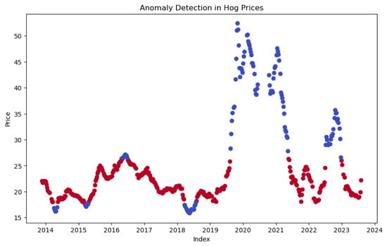
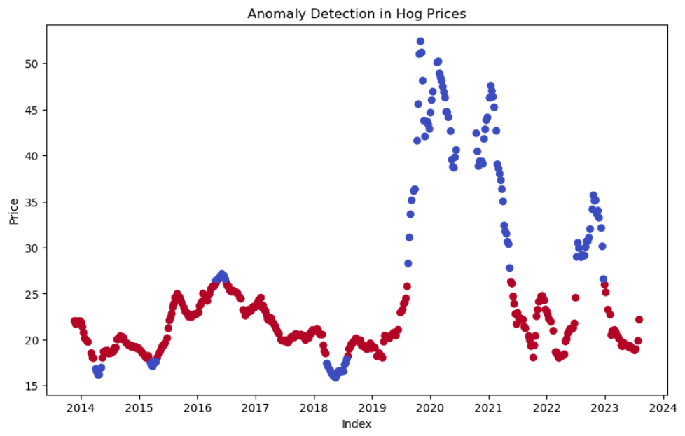
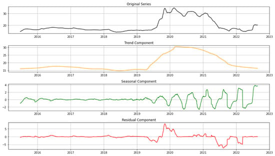
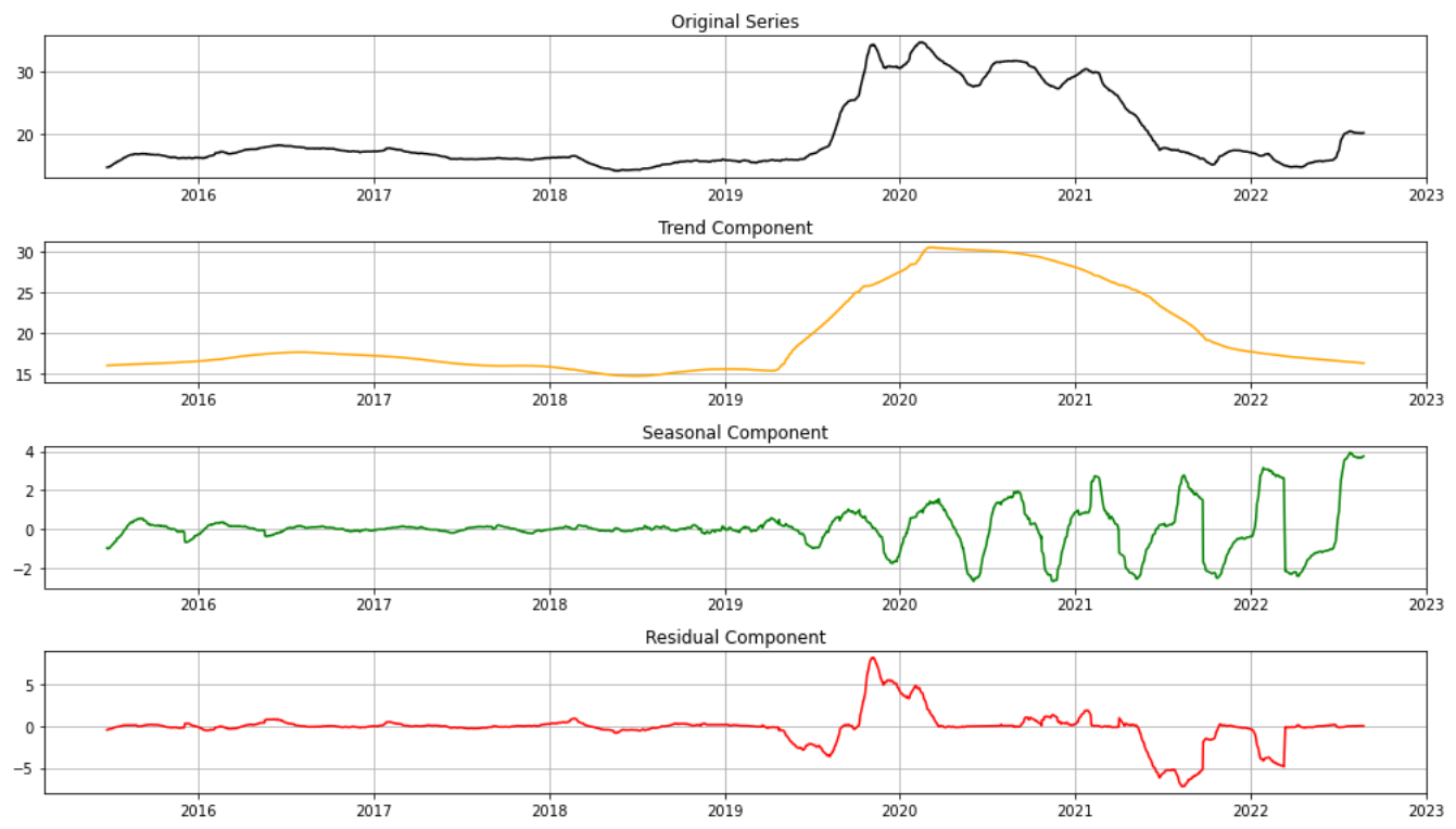
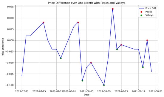
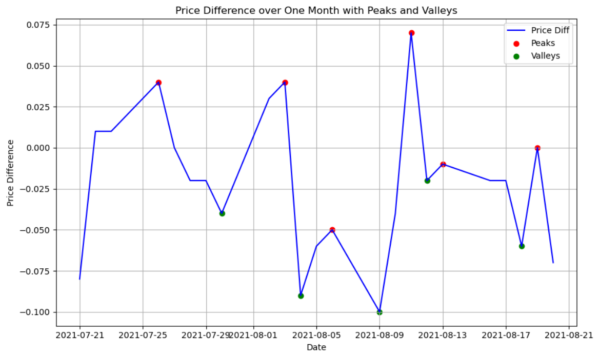
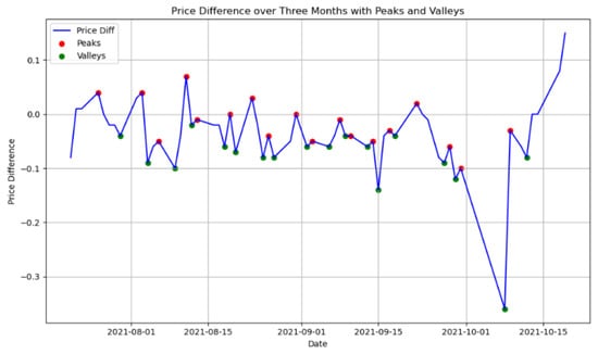
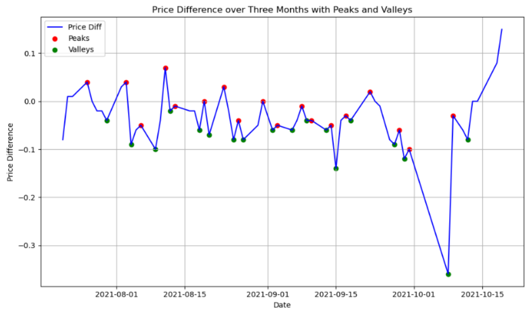
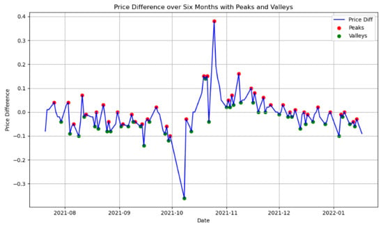
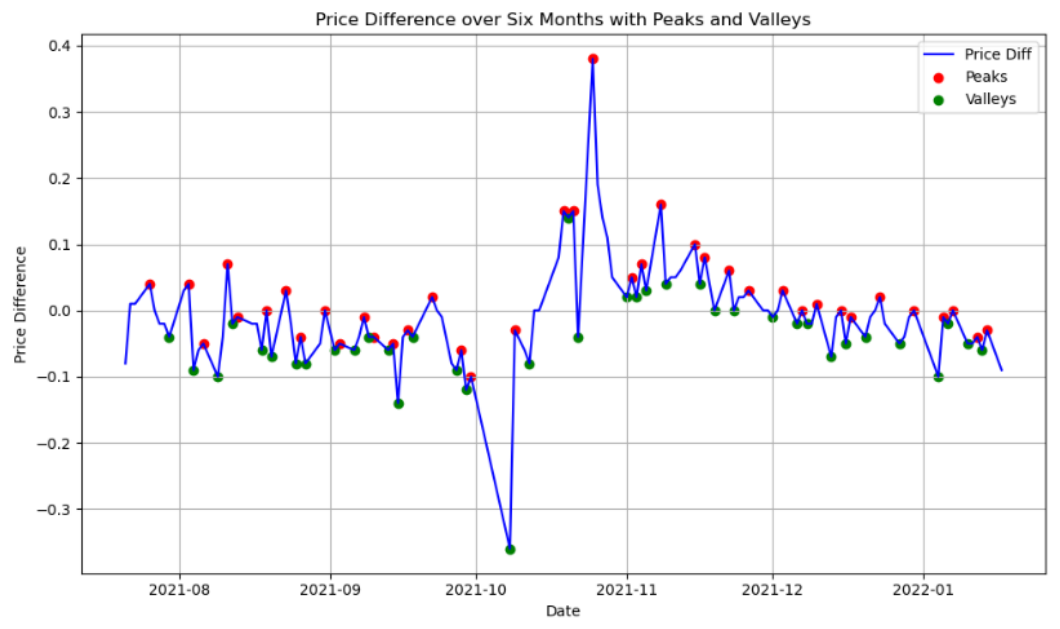
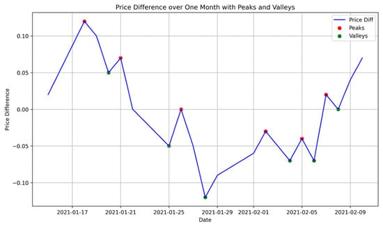
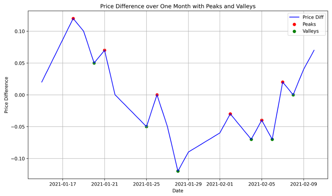
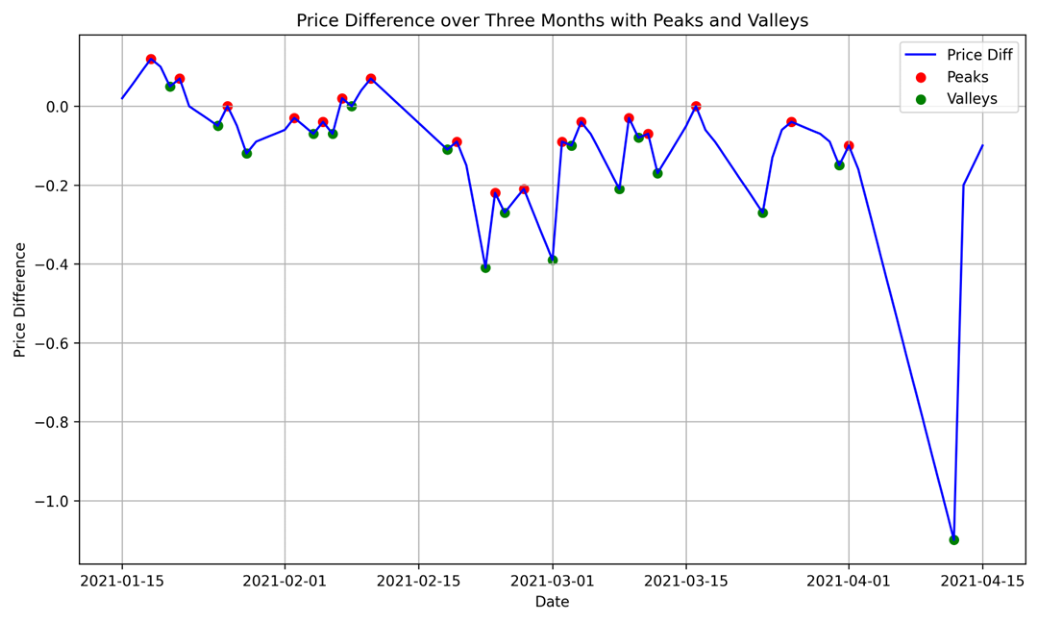
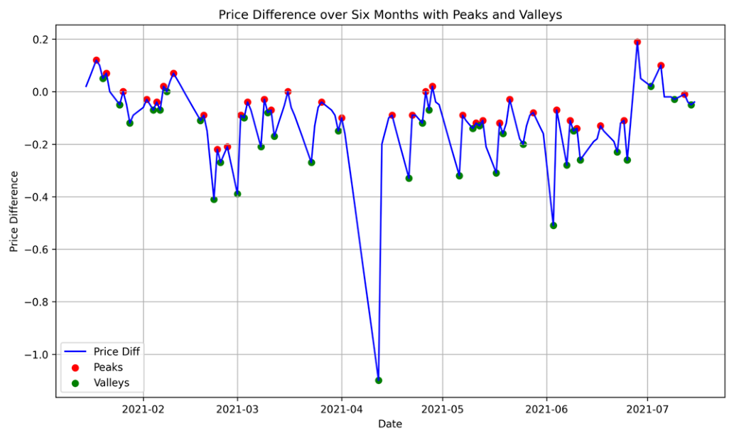
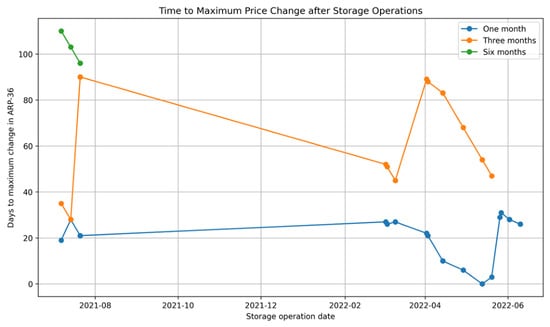
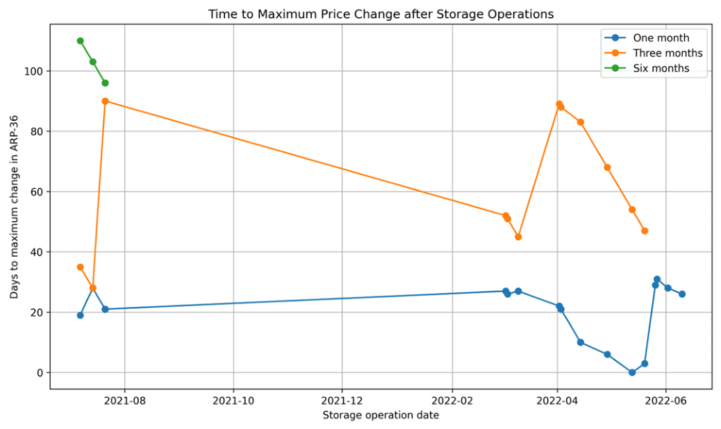
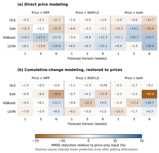
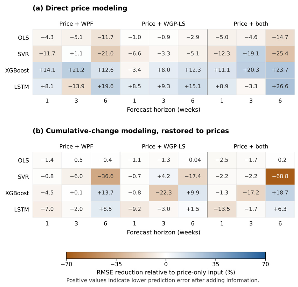

Disclaimer/Publisher’s Note: The statements, opinions and data contained in all publications are solely those of the individual author(s) and contributor(s) and not of MDPI and/or the editor(s). MDPI and/or the editor(s) disclaim responsibility for any injury to people or property resulting from any ideas, methods, instructions or products referred to in the content. |
© 2026 by the authors. Licensee MDPI, Basel, Switzerland. This article is an open access article distributed under the terms and conditions of the Creative Commons Attribution (CC BY) license.