


Abstract
Global warming has made climate physical and transition risks systemic sources of financial instability and key challenges to sustainability. These risks can spread to carbon, energy, and metals markets, which are central to the low-carbon transition and sustainable finance. This paper, therefore, explores the Quantile Time-Frequency connections among climate physical risk, climate transition risk, and the carbon, energy, and metals markets, with the analysis conducted through the lens of higher-moment risks. Using climate physical and transition risk indices together with daily carbon, energy, and metals futures settlement prices spanning 1 July 2015 to 29 December 2023, we employ the GJRSK model to extract higher-moment risk measures and apply the Quantile Time-Frequency framework to examine spillover effects across return, volatility, skewness, and kurtosis dimensions under different quantiles over the short term and long term. Furthermore, we construct a multilayer network that integrates information on return, volatility, skewness, and kurtosis risks under diverse market conditions and measure the topological properties of this network. The results reveal the following key insights: First, higher-moment risk spillovers are pronounced, though their magnitude is lower than that of return and volatility spillovers. Second, return, skewness, and kurtosis spillovers are primarily short-term driven, while volatility spillovers are concentrated in the long run. Climate risks generally act as receivers, but they shift to transmitters during long-term market downturns. Finally, findings from the multilayer complex network analysis demonstrate pronounced differences in the structural configurations of the interconnected networks linking climate risks to the return, volatility, skewness, and kurtosis risks of the carbon, energy, and metals markets across varying conditional quantiles. These findings support the measurement and monitoring of climate-related systemic risk and provide implications for sustainable finance, carbon and energy transition policies, and cross-market risk governance.
1. Introduction
The intensification of global warming has heightened the instability of the climate system, positioning climatic factors as a systemic risk to economic and financial stability and a major challenge to sustainable development [1,2]. The 2024 Global Risks Report identifies extreme weather events, critical shifts in Earth systems, and the loss of biodiversity alongside ecosystem collapse as the top three long-term risks. Furthermore, these risks are interconnected: abrupt and irreversible changes in Earth systems will trigger more frequent extreme weather events, thereby exacerbating climate-related risks. Climate risks primarily encompass physical risks (PRIs) and transition risks (TRIs) [3]. Specifically, climate physical risks refer to extreme natural climate events, such as hurricanes, droughts, floods, and heatwaves, that exert direct impacts on carbon, energy, and metal markets [4]. In contrast, climate transition risks denote losses arising from factors including climate policies, technological innovation, and investor market sentiment during society’s transition toward a low-carbon economy [5,6]. The Paris Agreement highlights that climate change risks exhibit spillover effects, and their impacts on economic and social activities are characterized by a long-term, widespread, and complex nature [7]. These observations have attracted substantial scholarly attention to investigating the effects of climate-related risks on carbon markets [8], energy markets [9,10], and metal markets [11,12,13].
Climate risks are intricately linked to metal, energy, and carbon markets, which are central to the low-carbon transition and sustainable finance [7,10]. Carbon dioxide emissions represent a key driver of climate change, while carbon emission trading markets serve as effective market-based solutions to mitigate climate change risks [14]. On one hand, extreme climate events impact market prices by disrupting both supply and demand dynamics. Extreme weather conditions, such as prolonged heatwaves or cold spells, increase the demand for air conditioning or heating, respectively, which in turn boosts energy consumption and drives up carbon emission prices [15]. Natural disasters like droughts or floods can disrupt energy and metal extraction and their associated transportation infrastructure, thereby causing supply breakdowns and price instability [16,17]. Conversely, initiatives related to the low-carbon economic transition—including shifts in climate policies and technological innovations—exert a considerable influence on development costs, which in turn impacts market supply chains and prices. Climate change may compel government authorities to formulate environmental policies related to carbon reduction, such as restricting fossil fuel consumption [18]. Such measures increase the costs of fossil energy development [19], reshape energy supply and demand, and affect energy market prices [20]. Additionally, they modify the supply of carbon emission allowances, thus affecting carbon prices [21,22]. Meanwhile, the low-carbon transition encourages the development of clean energy, which increases the demand for metal minerals [23]. However, metal extraction, in turn, contributes to higher carbon dioxide emissions [24]. A rise in carbon prices can, to a certain extent, reduce the proportion of metal extraction from raw ores, leading to price volatility in metal markets [24]. Additionally, given that carbon, energy, and metal markets possess financial attributes, climate risks can shape investor behavior and amplify market price volatility.
Among the extensive body of literature examining climate risks and their relationships with metal, energy, and carbon markets [25,26], considerable focus has been placed on probing the spillover impacts of climate risks on the return and volatility of carbon and energy markets. The findings of these studies consistently demonstrate the existence of significant spillover effects [27]. As for metal markets, research has mainly centered on the spillover impacts of climate risks on precious metal and energy metal market risks [12,28]. Nonetheless, a research gap persists in the systematic comprehension of the interactions between climate risks and these three markets (carbon, energy, and metal markets). Notably, metal, energy, and carbon markets are closely interconnected [29,30]. Integrating a broader set of markets into a unified systemic analytical framework can more effectively enhance the comprehension of climate risks’ comprehensive impacts, which in turn supports policymakers in formulating more appropriate climate risk policies and carbon trading market mechanisms. Although Zhou et al. (2023) [7] also investigated the connections between climate risks and the carbon, energy, and metal markets, their study concentrated more on the asymmetric impacts of climate risks on the overall spillover effects across these markets. Yet it failed to study the interlinkages of higher-moment risks between climate risks and each separate market.
On the other side, the existing literature has mainly centered on exploring climate risk impacts on return and volatility risks [31,32], yet it has paid inadequate attention to the spillover effects of higher-moment risks. This is rooted in the fact that, within financial markets, returns are conventionally employed to gauge a market’s overall performance, while volatility acts as an indicator for market risk [33]. Yet in practice, the volatility of carbon, energy, and metal markets exhibits considerable complexity. These markets are highly vulnerable to the dual effects of internal and external factors (e.g., extreme events and investor sentiment) [34], which in turn gives rise to excess kurtosis and fat-tailed distributions [33]. These traits cannot be completely captured by lower-order moments, but they can be effectively reflected via higher-order moments [35,36]. A large body of research has demonstrated that higher-moment risks constitute a crucial component of financial market risks [37], and their impacts on asset pricing and volatility modeling should not be underestimated [38]. Furthermore, the interconnected relationships between different financial assets are not only manifested in their first moments but also exhibit reflections in second moments and even higher moments [33]. Thus, the measurement of risk spillover effects ought to encompass not only lower-order moments but also incorporate considerations of spillover effects at the higher-moment level. Specifically, the results of skewness spillovers can shed light on how asymmetric risks propagate between climate risks and the metals, energy, and carbon markets, whereas the results of kurtosis can clarify whether and to what degree extreme events in these markets spill over to climate risks [39]. Cui and Maghyereh (2025) [26] investigated the connectedness of higher-moment risks between climate risks and the carbon and energy markets, with their results revealing that such connectedness outcomes hinge on specific quantile levels and moment orders. Drawing on this line of research, the present study places emphasis on integrating metals markets into the analytical framework, while focusing on an examination of the spillover impacts of climate risks on the return, volatility, skewness, and kurtosis risks within the metal, energy, and carbon markets.
Moreover, considering that the effects of climate risks on the short-term and long-term risks of metal, energy, and carbon markets vary [40], as are their risk impacts under different market conditions [41], this research utilizes the Quantile Time-Frequency model to comprehensively examine the short-term and long-term multi-dimensional risk spillover effects of climate risks on metal, energy, and carbon markets under diverse market conditions. Building on the analysis of spillover effects, a large body of literature has constructed single-layer networks to explore the risk contagion relationships between markets [41,42]. However, such single-layer network structures are unable to fully capture the diversity and heterogeneity inherent in information transmission and market interlinkages [43] while also neglecting the asymmetric effects of investor sentiment on positive versus negative returns [44]. Although some studies have developed multilayer networks [45,46], these networks are primarily limited to information on returns, volatility, and extreme risks [47] or consist of 2–4 hierarchical structures based on different time periods, with insufficient attention paid to more complex networks with higher hierarchical levels. Considering that the risk contagion networks of returns, volatility, skewness, and kurtosis all exhibit connectivity under different market conditions, this study adopts a multilayer network approach to construct a 12-layer information network. This network encompasses layers for returns, volatility, skewness, and kurtosis, as well as risk layers corresponding to upper, lower, and median conditional quantiles. Such a network structure plays a pivotal role in facilitating an in-depth understanding of the interplays among climate risks, carbon markets, energy markets, and metals markets. We define a set of indicators to quantify and evaluate the network’s characteristics at both the systemic level and the market-specific level, aiming to provide valuable information for the decision-making of investors and regulators.
Building on the above discussions, this paper makes the following key contributions: First, while the existing literature has separately focused on the connections between climate risks and energy markets [48,49], the interplay between climate risks and metal markets [13,28], the interconnections among metal, energy, and carbon markets [29,30], the holistic dynamics involving climate risks, and the carbon–energy–metal system remain insufficiently explored. This research strives to evaluate the complex interrelationships between climate risks and the metal, energy, and carbon markets, and it opens up a new research avenue by exploring the risk contagion relationships in cross-market systems. Second, from a methodological perspective, we integrate the higher-moment model with the Quantile Time-Frequency model to investigate the intensity of spillover effects between climate risks and the return, volatility, skewness, and kurtosis-related risks of the metal, energy, and carbon markets under different market scenarios and across various time-frequency domains. This integration enables a more effective identification of short-term and long-term spillover systems associated with both extreme negative and positive impacts, thereby providing insights into the intertemporal dependence structure of tails [50] and enabling a thorough comprehension of the characteristics of spillover effects between climate risks and cross-market systems. Third, this study constructs a multilayer network that encompasses return, volatility, skewness, and kurtosis risks under extreme market upside, extreme market downside, and normal market conditions. By exploring the multi-dimensional risk contagion paths between climate risks and carbon, energy, and metal markets, this network provides more valuable information for regulators to prevent risks. Within a multilayer network, the links in each individual layer denote distinct types of connections among the same set of nodes (in this case, climate risks and carbon, energy, and metal markets). This design allows for the comprehensive application of multiple interconnectivity indicators, thereby effectively describing the complex financial system—not only covering the return dimension but also simultaneously presenting other risk metrics [2].
Aiming to provide implications for sustainable market risk management and low-carbon transition, this study examines how climate physical and transition risks interact with carbon, energy, and metals markets across return, volatility, skewness, and kurtosis risks, and how these interactions evolve across conditional quantiles, time horizons, and network structures. The remainder of this paper is structured as follows. In Section 2, we provide a survey of the relevant literature related to climate risk spillover effects. Section 3 elaborates on the GJRSK and Quantile Time-Frequency methodologies and simultaneously presents the data sources as well as descriptive statistical analysis. Section 4 reports the empirical results, while Section 5 reaches conclusions for the study.
2. Literature Review
With the influence of climate risks on financial markets growing stronger, an increasing number of researchers have started focusing on the spillover impacts of climate risks on the metal, energy, and carbon markets [10,11,50]. Table 1 presents the relevant literature on spillover effects among climate risks and the metal, energy, and carbon markets, organized by author, methodology, key markets studied, time period, and main findings. From the perspective of market selection in existing studies, the focus on carbon, energy, and metal markets varies by research perspective when centered on climate risks, and they can be specifically categorized into four types. Initially, in terms of climate risk indicators, existing studies primarily focus on two broad risk categories. One is policy-driven risks, with the Climate Policy Uncertainty (CPU) index as the dominant measure [13,32]. A growing strand of research uses text-based physical and transition risk indices or climate-related attention measures, such as the Climate Physical Risk Index and the Climate Transition Risk Index constructed by Bua et al. (2024) [51], or climate risk attention indicators. Additionally, studies covering the energy market encompass both traditional and clean energy sectors, though the former has received greater research attention. For traditional energy, crude oil, natural gas, and coal are high-frequency research targets [10,31,49]. This is because these energy sources have direct links to carbon emissions and are highly sensitive to climate policies. For clean energy, studies mostly focus on solar energy, wind energy-related indices, and clean energy ETFs [28,52]—a reflection of the positive driving role of climate policies in the clean energy industry. Furthermore, in the carbon market, the Global Carbon Index is the most widely used indicator [28,53]. Some studies also incorporate regional carbon market prices (e.g., China’s national carbon price), but global indices remain the primary focus. Recent work by Cui and Maghyereh (2025) [26] further extends this analysis to higher-moment spillovers across climate risk, carbon, and fossil fuel markets. Lastly, for metal and related commodity markets, the selection of metal types is directly tied to “energy transition demand”, with a focus on industrial metals, such as copper, aluminum, and nickel [28]. These metals serve as critical raw materials in the new energy industrial chain and have direct connections to climate policies. Precious metals are included less frequently, despite recent evidence showing that their correlations with climate risks differ from those of non-ferrous metals. Recent studies have further expanded this line of research to examine carbon, energy, and metal markets as an interconnected system. Hong et al. (2026) [54] identify long-run cointegration and show that spillovers and co-movements intensify during crisis periods. Wu and Huang (2025) [40] further demonstrate that connectedness within this system is stronger in tail conditional quantiles and dominated by short-term dynamics, with metals, especially copper, playing a central role. Chu et al. (2026) [55] extend the market set to rare earths and document tail risk transmission that differs across time-frequency domains. Although these recent studies increasingly treat carbon, energy, and metals as an interconnected system, they generally focus on return or volatility connectedness, restrict metals to industrial or energy transition metals, or omit the simultaneous quantile frequency and multilayer dimensions. None of them combines higher-moment risks, physical and transition risks, a metal set covering both precious and non-ferrous metals, and multilayer network structures in a single framework. To address this gap, this study incorporates climate physical risk, climate transition risk, the carbon market, the metal markets, and the energy market into a single system. The energy markets in this framework include both traditional and clean energy, while the metal market covers both precious metals and non-ferrous metals.
From the perspective of research methodologies, to better accommodate the complex characteristics of climate risks, the existing literature has primarily employed three key approaches derived from the spillover index framework proposed by Diebold and Yilmaz (2012, 2014) [56,57]: the quantile VAR model developed by Ando et al. (2022) [58] (QVAR model), the time-varying parameter VAR approach by Antonakakis and Gabauer (2017) [59] (TVP-VAR model), and the frequency connectedness method by Baruník and Kehlík (2018) [60] (BK model). Recent applications have combined these approaches to examine climate risk spillovers under extreme conditions and across time-frequency dimensions [28,42,52,61]. Among these, the QVAR model has the highest adoption rate [10,11]. This popularity can be attributed to its core advantage: it overcomes the limitations of traditional “mean reversion” frameworks and captures spillover effects under extreme market conditions. For instance, Khalfaoui et al. (2022) [25] used this model to find that the connectedness of climate-related indices is considerably stronger during “extreme upper and lower quantiles” than the median quantile. The second category of widely adopted methodologies includes the TVP-VAR model and the BK model [49,61]. The TVP-VAR model permits the time-varying evolution of parameters, thereby facilitating the accurate characterization of how spillover effects evolve dynamically. For example, Hoque et al. (2023) [8] applied the TVP-VAR frequency connectedness method to examine the frequency-based linkages and spillovers between climate factors, carbon, and energy markets, revealing that spillover magnitudes differ between short and long terms and exhibit time-varying properties. To distinguish between spillover differences arising from “short-term fluctuations” and “long-term trends”, the BK model [47,53] can be combined with the DY model to form a time-frequency analytical framework, facilitating a more nuanced analysis of spillover variations across short, medium, and long terms. Rao et al. (2023) [4], for instance, found that the CPU acts as a net transmitter of energy price shocks within a 1–3 month horizon, as short-term policy uncertainty tends to trigger speculative behavior in energy markets. Liu et al. (2025) [27] used the BK model to demonstrate that climate transition risks exert long-term spillovers on the “carbon-energy-stock” system, given that transition risks reshape the long-term investment logic of the energy sector. Some studies have further optimized the VAR framework. For example, Cui and Maghyereh (2025) [26] proposed the QVAR extended joint connectedness approach, which incorporates a moment order dimension, while Ren et al. (2025) [31] developed the LASSO-VAR-DY spillover index, which uses LASSO regularization to reduce variable redundancy and improve analytical accuracy for high-dimensional markets. Liu et al. (2025) [62] further examine higher-moment risk spillovers between carbon and energy markets under climate policy uncertainty, finding that higher-order spillovers are weaker than lower-order ones but intensify under extreme risk states. A small number of studies have adopted more specialized tools, such as the TENET model by Deng et al. (2025) and the R2 decomposition connectedness method by Yang et al. (2025) [63]; however, these methods account for a small share of the literature and have not yet become mainstream. In parallel, network-based studies have progressed from single-layer graphs to multilayer structures, in which different moments or frequencies form separate layers [45,46,64].
Building on existing findings, two key stylized facts have emerged: (1) the nonlinear characteristic that connections between climate risks and various markets strengthen considerably in extreme market scenarios [10,25]; and (2) significant time-frequency differences in spillover effects, with short-term spillovers driven by sudden policy shocks [4] and long-term spillovers dominated by structural changes [65]. The QVAR model and BK model alone cannot simultaneously account for spillover differences across both market conditions and frequency dimensions. Thus, combining these two models is essential to accurately capture the dynamic features of market spillovers across different frequency dimensions in extreme market scenarios [66]. Building on the methodological insights from Adeabah and Pham (2025) [10] and He et al. (2025) [67], this research employs the Quantile Time-Frequency approach (QVAR-BK model) to analyze the interlinkages between climate risks and the metal, energy, and carbon markets in various conditional quantiles and across various frequency bands. Overall, whether a market or climate risk index acts as a transmitter or receiver is not fixed; it depends on the moment, quantile state, frequency band, and market sample considered. This conditional nature of transmission roles motivates a framework that jointly accounts for higher moments, conditional quantiles, time horizons, and multilayer network structures.
Furthermore, it is noteworthy that the existing literature has predominantly focused on exploring the spillover relationships between climate risks and either the returns or volatility of various financial markets, while paying insufficient attention to the connections between climate risks and higher-moment risks in these markets. For instance, He et al. (2025) [67] explored the spillover impacts connecting the CPU with the return performance of energy and stock markets. Ren et al. (2025) [31], in turn, explored the dynamic connectedness between climate risks, oil shocks, and the returns of energy futures markets. However, the role of higher-moment risks in the transmission of climate risks to financial market risks should not be underestimated. This is because higher-moment risks can capture asymmetry, tail risks, and extreme volatility—factors that are difficult to measure using traditional risk metrics, yet they are critical for understanding market behavior during crises or periods of abnormal fluctuations [68]. Although Cui and Maghyereh (2025) [26] investigated higher-moment risk spillovers across climate risks, renewable energy markets, carbon, and fossil fuel markets, their analysis was conducted across different quantiles. Our study differs from theirs in two key aspects: on the one hand, we further incorporate the dimension of frequency to study the connectedness between climate risks and financial markets under quantile-based spillovers; on the other hand, we include both energy, metal, and precious metal markets in our analysis. Accordingly, this study incorporates the GJRSK model to examine the short- and long-term spillover effects between climate risks and the return, volatility, skewness, and kurtosis risks of the metal, energy, and carbon markets in extreme market scenarios.
To address these issues, we first examine the existence and magnitude of spillovers between climate physical and transition risks and carbon, energy, and metals markets across the return, volatility, skewness, and kurtosis dimensions. We then assess how these spillovers differ between median and tail conditional quantiles and between short- and long-term horizons. In addition, we identify the primary transmitters and receivers within the climate risk–carbon–energy–metals system.
Table 1.
Summary of relevant studies on spillovers among climate risk, carbon, energy, and metal markets.
3. Methodology and Data
3.1. Higher-Order Moment Risk Measure
Financial time series exhibit typical characteristics such as fat tails, leptokurtosis, and leverage effects. To quantify the conditional volatility, skewness, and kurtosis, this study adopts the GJR–skewness–kurtosis (GJRSK) model developed by Nakagawa and Uchiyama (2020) [76]. Its specific mathematical expression is presented as follows:
where ηt|It−1 ∼ g(0, 1, st, kt) and It−1 is the information set available at time t − 1. g(0, 1, st, kt) represents a probability density function characterized by a mean of 0, a variance of 1, a skewness of St, and a kurtosis of kt. Additionally, rt denotes the return vector of metal, energy, and carbon markets, calculated as 100 × (Pt − Pt−1)/Pt−1, where Pt stands for the daily closing market indices of the respective markets.
3.2. Quantile Time-Frequency Connectedness Method
By integrating the BK model proposed by Baruník and Kehlík (2018) [60] with the quantile connectedness approach developed by Marco et al. (2023) [77], this study examines the quantile-based propagation effects among climate risk, metal, energy, and carbon markets across distinct frequency bands. The computation of connectedness metrics requires the estimation of a quantile vector autoregressive (QVAR) model, whose mathematical form is specified as follows:
where p represents the lag length of the QVAR model xt and xt−i (i = 1 … p) denote N × 1 dimensional variable vectors. Let τ stand for the quantile, μt(τ) represent the conditional mean vector, ut(τ) represent an error vector with an error variance–covariance matrix, Ξ(τ), and Θi(τ) denote a QVAR coefficient matrix that varies with the quantile τ. To transform the QVAR (p) model to its QVMA(∞), we rely on Wold’s theorem:
xt = μt(τ) + Θ1(τ)xt−1 + Θ2(τ)xt−2 + ⋯ Θp(τ)xt−p + ut(τ)
The core element of the connectedness methodology resides in the generalized forecast error variance decomposition, which acts as the cornerstone for examining the transmission mechanisms of shocks across different markets:
where H denotes the forecast horizon. To make different comparable, they are standardized as follows:
To operationalize this quantification, the total connectedness index (TCI) is defined as follows:
Subsequently, this methodology enables the quantification of the magnitude of the transmission effect from market k to all other remaining markets, denoted as “total spillover effect on other markets (TO)”:
Likewise, it allows for the quantification of the magnitude of spillover effects that market k absorbs from all remaining markets, referred to as “total spillover from other markets (FROM)”:
Subsequently, the net spillover (NET) is derived as:
NETk(H) = TOk(H) − FROMk(H)
Then, this study computes the net pairwise spillover index (NPDC):
Building on Equation (10), this study constructs a matrix , where α = 1, 2, 3, 4, 5, 6, 7, 8, 9, 10, 11, 12 correspond to the return, volatility, skewness, and kurtosis networks under the 0.1, 0.5, and 0.9 quantiles, respectively, where 0.1, 0.5, and 0.9 quantiles denote the lower, median, and upper conditional quantiles of the corresponding risk dimension. Since the spillover matrix inherently contains noisy components, an appropriate threshold is selected to implement a filtering procedure for the matrix.
Furthermore, the present research utilizes the BK model to investigate the spectral behavior of the variables under investigation.
where , , and w stand for the frequency. SX(ω) serves as a core tool for characterizing dynamic frequency characteristics, describing the distribution of the sequences Xt across different frequency components ω. For a given ω ∈ (−π, π), the generalized causation spectrum can be formally defined as:
where denotes the component of the spectrum of the j-th series. We can derive a comprehensive indicator of connectedness, d = (a, b): a, b ∈ (−π, π):
Against this methodological backdrop, this study leverages these analytical measures to characterize the dynamics of frequency-based spillovers, thereby providing insights into how effects transmit across distinct frequency intervals:
NETk(d) = TOk(d) − FROMk(d)
To dissect the temporal heterogeneity of risk spillovers, this study delineates two distinct frequency bands and subsequently examines the risk transmission across short-term and long-term horizons. Among these bands, d1 = (π/22, π) denotes the high-frequency band, corresponding to the short term (1–22 days); meanwhile, d2 = (0, π/22) denotes the low-frequency band, corresponding to the long term (over 22 days). This division not only aligns with the typical time scales of market participants’ decision-making (e.g., short-term arbitrage vs. long-term investment) but also enables a targeted analysis of how risk spillovers evolve across different temporal dimensions.
3.3. Multilayer Network Measures
Let V = {1, 2, … N} denote the set of nodes, where each element corresponds to climate risk or the metal, energy, and carbon markets. On this basis, we define a single-layer network as G[α] = G(V, Cα). This study includes 12 layers in total, covering the return, volatility, skewness, and kurtosis layers under the 0.1, 0.5, and 0.9 quantiles, respectively, with each layer comprising 14 nodes. For a given threshold of layer α, and using to filter the noisy information contained in Cα, the element in the adjacency matrix is defined as:
Since variance decomposition generates a fully connected network, this characteristic obscures critical interconnected information [1]. To eliminate redundant or noisy information in each network layer, this paper adopts a threshold method to screen the fully connected network, retaining the most critical interconnected information. Following the approach of Chen and Wang (2025) [78], we select the element at the 0.13th quantile as the threshold, removing edges below this threshold. Ultimately, we obtain the filtered multilayer information spillover networks and .
3.3.1. System-Level Measures
(1) Single-level network measures. First, we incorporate global efficiency (GE), a measure proposed by Latora and Marchiori (2001) [79], to measure the information exchange efficiency within the network. For layer α (where α denotes any of the 12 filtered single-layer networks, e.g., the return volatility layer under the 0.1 quantile or the skewness layer under the 0.9 quantile), its GE is defined as follows:
GE measures the efficiency with which risk information is exchanged across the network. A higher GE indicates shorter average transmission paths, so risk information can reach other markets with fewer intermediate steps. Conversely, a lower GE reflects longer or more fragmented transmission paths, indicating less efficient information exchange across markets.
Among them, denotes the shortest path from node j to node k in layer α. A higher GE value indicates more effective information exchange. Second, we adopt the average connectedness strength (ACS) in layer α, which measures the average strength of pairwise spillovers within the network. A higher ACS indicates that direct risk linkages between markets are stronger, whereas a lower ACS indicates weaker pairwise linkages. The ACS can be written as:
(2) Multilayer network measures. Following Artime et al. (2021) [64], we introduce the indicators of edge overlapping, deg-deg Pearson, deg-deg Spearman, and shortest paths to characterize the correlation between layers. The edge overlapping (Eα,β) indicator measures the degree of shared edges between different layers in a multilayer network. Specifically, if the same pair of nodes has edges in multiple layers, these edges are considered shared across the layers. The higher the edge overlapping degree, the more similar the connection structures between the layers. This indicator helps to understand the relationships and similarities between different layers in a multilayer network.
where m(⋅) is a function that returns the minimum values of two tensors. denotes the adjacency tensor of the network, where ωab represents the interaction weight between node a and node b; denotes the normalized basis tensor, which corresponds to the rows and columns of the tensor product of the normalized vectors of node a and node b, respectively, with the basis here referring to the Euclidean basis. is a 2nd-order “1-tensor,” i.e., all its components are equal to 1.
Inter-layer assortativity is an indicator that measures the degree to which nodes with the same or similar attributes connect to one another in a network. In a multilayer network, calculating the assortativity between different layers facilitates an understanding of the correlation in node attributes across these layers. The deg-deg Pearson and deg-deg Spearman correlation coefficients are two important indicators to describe interlayer homogeneity. The deg-deg Pearson correlation coefficient (, hereafter referred to as deg-deg Pearson) utilizes the Pearson correlation coefficient to measure the correlation in node degrees (i.e., the number of connections per node) between different layers. Specifically, for the Pearson correlation coefficient, the magnitude of its absolute value directly reflects the strength of the correlation: the closer the absolute value is to 1, the greater the strength of the correlation; conversely, the closer the absolute value is to 0, the weaker the correlation.
where denotes the multi-degree of node j in layer α, and represents the corresponding average in multi-degree across in layer α. The value of RP ranges between −1 and 1. To conduct robustness tests, this paper further introduces the deg-deg Spearman correlation coefficient (). This indicator measures the correlation in node degrees between different layers using the Spearman correlation coefficient, which is based on ranks rather than raw data and is not affected by extreme values, making it more robust in empirical analyses. Here, dj denotes the difference between these two rank values of and .
Shortest path similarity is an indicator that measures the similarity in the shortest path lengths between node pairs across different layers of a multilayer network. Specifically, if there is high similarity in the shortest path lengths between the same node pairs across different layers of the network, these layers will exhibit high structural similarity. This indicator facilitates an understanding of the similarity in the global topological structures across different layers of the multilayer network. Let denote the shortest path between any two nodes j and k in layer α. Then, , and the formula for inter-layer shortest path similarity can be expressed as:
3.3.2. Market-Level Measures
According to the studies by Dai et al. (2023), the average overlapping in-strength (Oin), average overlapping out-strength (Oout), and average overlapping net strength (Onet) are employed to characterize the connectivity of nodes [47]. These indicators, respectively, correspond to the average in-market strength, out-market strength, and net market strength of each individual market across all layers. Their mathematical expressions are presented as follows:
where ISM denotes the in-strength of market j (), OSM represents the out-strength of market j (), and NSM stands for the net strength of market j ().
3.4. Data Descriptions
In investigating the spillover effects between climate risk and the energy, carbon, and metal markets, we adopt the daily indices of the Climate Physical Risk Index (PRI) and the Transition Risk Index (TRI), developed by Bua et al. (2024) [51], to proxy for climate risk. This index set has been widely utilized in scholarly research [32], with access to the data provided via http://www.policyuncertainty.com (accessed on 30 June 2024). For the carbon market variable, we select the daily futures pricing data of the ICE-EUA futures contract (EUA). To construct uninterrupted data, we use the daily settlement prices from the one-year window preceding the expiration of each carbon futures contract, following the approach of Zhang and Sun (2016) [80]. Drawing on Zhou et al. (2023) [7], our energy market proxies include three key indicators: the futures prices of Brent crude oil (Oil) and natural gas (Gas) traded on the London International Petroleum Exchange (IPE), as well as the S&P Global Clean Energy Index (CEI) [7]. Regarding the metal market, we incorporate two categories of futures: six non-ferrous metals (copper, tin, lead, nickel, aluminum, and zinc) traded on the London Metals Exchange (LME), and two precious metals (gold and silver) listed on the New York Commodity Exchange (COMEX) [64]. Specifically, we utilize the daily returns of LME 3-month futures contracts, as these are recognized as the most liquid metals futures instruments globally [80]. Except for climate risk indicators, all other datasets are sourced from the WIND database. Due to incomplete records of natural gas prices in 2014 [80], our sample period is set from 1 July 2015 to 29 December 2023. We further restrict the sample to dates with complete pricing data across all markets. Additionally, the oil and nickel markets exhibited outliers on specific dates: the oil and nickel markets exhibited extreme observations on 20–21 April 2020 and 7 March 2022, respectively. These episodes represent extraordinary market dislocations rather than ordinary tail events: the first-ever negative WTI settlement on 20 April 2020 reflected the near exhaustion of available storage capacity at Cushing, while the extreme nickel price surge beginning on 7 March 2022 prompted the LME to suspend trading on the following day. Including these observations could disproportionately influence higher-moment estimates and obscure the underlying spillover relationships. We, therefore, excluded these three trading dates from all market series to maintain a balanced panel. Ultimately, we compute percentage returns for all fourteen assets as 100 × (Pt − Pt−1)/Pt−1, with each series comprising a total of 1635 observations. All data processing and empirical analyses were performed using R version 4.4.0.
Table 2 presents the minimum (Min), maximum (Max), median, mean, standard deviation (Std.Dev), kurtosis, skewness, the augmented Dickey–Fuller (ADF) stationarity test, and the Jarque–Bera normality test (J-B) results for the returns of the metal, energy, and carbon markets, as well as the climate risk indicators. As shown in Table 2, the aluminum and tin markets have negative mean returns within the sample period, indicating that these markets experienced a decline in price performance during the period. In contrast, the remaining markets exhibit positive mean returns. In terms of standard deviation, the natural gas market returns display the highest volatility, while the PRI and TRI indices show relatively low volatility. From the results of skewness and kurtosis, most markets display leptokurtic (sharp-peaked) and fat-tailed characteristics. The J-B statistic further confirms the non-normal distribution of all indicators. To verify data stationarity, this study employs the ADF test, and the results indicate that all selected indicators exhibit stationarity at the 1% statistical significance level.
Table 2.
Statistical summary of all return series.
Figure 1 presents the pairwise correlation heatmap between climate risk and the returns of the energy, carbon, and metal markets. Within this heatmap, the deeper the shade of blue, the more intense the positive correlation between two markets, whereas the richer the red hue, the more pronounced the negative correlation. As observed in Figure 1, the correlation between precious metals markets and climate risk is considerably higher than that between non-ferrous metals markets and climate risk. Additionally, the correlation between CEI returns and climate risk is stronger than that between returns of the traditional energy (Brent crude oil) market and climate risk. Notably, the Climate Transition Risk Index exhibits a markedly stronger correlation with natural gas market returns than the Climate Physical Risk Index, indicating that the natural gas market is more susceptible to climate transition risk. However, for the carbon market, its correlation with the PRI is stronger. Compared with the metal markets, the carbon market maintains closer ties with the energy markets. Within the metals markets, the carbon market exhibits a notably stronger correlation with non-ferrous metals markets than with precious metals markets.
Figure 1.
Heatmap for pairwise correlation coefficients of returns of each market.
4. Empirical Results
Building on the analysis of the static and dynamic connectedness between climate risk and returns, volatility, skewness, and kurtosis of the metal, energy, and carbon markets, this study constructs a multilayer network to explore the evolutionary characteristics of interconnectedness between climate risk and these markets.
4.1. Static Spillover Effects
To analyze market interconnections from a multi-dimensional perspective, this study employs the GJRSK model to calculate the volatility, skewness, and kurtosis of each market, with the results presented in Figure 2. As can be clearly observed from the figure, during periods such as the COVID-19 pandemic, the clean energy, oil, and metal markets experienced heightened volatility, indicating that market shock events exacerbate volatility risks in the metal and energy markets. From the perspective of higher-moment risk dimensions, the skewness and kurtosis curves of the natural gas, crude oil, and tin markets exhibit relatively stable fluctuations, with abrupt changes only occurring during the Russia–Ukraine conflict and the COVID-19 period. In contrast, the curves of other markets display a long-term pattern of unstable fluctuations. This suggests that higher-moment risk indicators are more capable of capturing the impacts of unexpected shocks on the metal, carbon, and energy markets, even extreme ones. To examine the interconnections among climate risk, the metal, energy, and carbon markets more comprehensively, we utilize the QVAR method to derive spillover matrices at the extreme upper (90th), extreme lower (10th), and intermediate (50th) quantiles. The lag order of the QVAR model is established as 1 based on the Akaike Information Criterion (AIC), and the horizon for prediction error decomposition is set to 10. From a dual time-frequency perspective, Table 3, Table 4, Table 5 and Table 6 report the static spillover matrices of return, volatility, skewness, and kurtosis risks across climate risk, the metal markets, the energy market, and the carbon market in normal market conditions. Here, the values of the main diagonal elements represent the respective self-contributions of each variable.
Figure 2.
Return, variance, skewness, and kurtosis of different markets.
Table 3.
The net return spillover effects across different frequency domains.
Table 4.
The net volatility spillovers across different frequency domains.
Table 5.
The net skewness spillovers across different frequency domains.
Table 6.
The net kurtosis spillovers across different frequency domains.
Comparing the correlation results in Figure 1 with the static spillover analysis, the latter reveals that climate risk has stronger linkages in the return dimension. The correlation heatmap measures contemporaneous linear associations, capturing whether climate risk indices and market returns move in the same direction within the same trading day, whereas the static spillover analysis summarizes directional connectedness among markets. This difference suggests that contemporaneous correlations alone may not fully capture market interconnectedness and supports the use of a spillover-based perspective.
Figure 3, Figure 4, Figure 5 and Figure 6 present the static connectedness between climate risk and the return, volatility, skewness, and kurtosis risks of the metal, energy, and carbon markets under the median conditional quantile (0.5). The static spillover indices and the spillover indices across different frequency domains are provided in Appendix Table A1, Table A2, Table A3 and Table A4. First, overall, the total spillover indices between climate risk and the various moments (returns, volatility, skewness, and kurtosis) of the metal, carbon, and energy markets are 44.71%, 45.55%, 24.07%, and 26.66%, respectively. This indicates substantial interconnectedness between climate risk and these markets. While the connectedness of kurtosis and skewness is notably lower than that of returns and volatility, the higher-moment spillover indices remain non-negligible in magnitude. This suggests that market regulators and investors should pay equal attention to risk spillovers at the higher-moment level. This outcome can be attributed to the global community’s collective efforts to address climate change, coupled with the growing prominence of the financial attributes of the metal, energy, and carbon markets [66]. Notably, the total spillover index does not decrease with an increase in moments. This conflicts with the conclusions of Wang et al. (2025) [34], who contended that spillovers from skewness and kurtosis are greater than those associated with lower-order moments. Additionally, the risk transmission values on the diagonal elements are generally greater than the risk reception values on the off-diagonal elements, indicating that each market is more strongly influenced by its own lagged risks.
Figure 3.
Static return spillovers in the 0.5 quantile. Notes: The “Spillover” color bar indicates the spillover intensity of the static spillover matrix, increasing from right to left. The TO and FROM bars are uniformly shown in blue: the right bars represent the total spillovers received by each market (FROM), and the bottom bars represent the total spillovers transmitted by each market (TO).
Figure 4.
Static volatility spillovers in the 0.5 quantile. Notes: For details, refer to the note accompanying Figure 3.
Figure 5.
Static skewness spillovers in the 0.5 quantile. Notes: For details, refer to the note accompanying Figure 3.
Figure 6.
Static kurtosis spillovers in the 0.5 quantile. Notes: For details, refer to the note accompanying Figure 3.
Secondarily, in terms of varying frequencies, the risk spillover impacts linked to returns, kurtosis, and skewness are far greater under high-frequency conditions than under low-frequency conditions. This points to the fact that the risk spillovers of returns, kurtosis, and skewness between climate risk and the carbon–energy–metal system are driven primarily by high-frequency spillovers, with inter-market spillover effects occurring mainly in the short term. This phenomenon may be ascribed to the reality that market participants are dominated by short-term speculation [30]. It also implies that climate risk and the returns, kurtosis, and skewness risks of metal, energy, and carbon markets are less affected by external shocks in the low-frequency bands, providing strong evidence for the feasibility of achieving diversified and stable returns in the long term [83]. In contrast, the volatility risk spillover indices come in at 14.01% (high-frequency band) and 31.54% (low-frequency band), signaling that inter-market volatility risk spillover effects predominantly take place over the long term.
Thirdly, in terms of directional spillover indices, markets with high levels of risk outflows often also experience high levels of risk inflows. Across all moments and frequency bands, the markets ranking among the top two in both risk outflows and inflows are concentrated in the metal markets. This indicates that metal markets occupy an information-leading position in the “climate risk-carbon-energy-metal” system. They serve as the main source of risk transmission resonance, while also exhibiting high sensitivity to risks and thus being more susceptible to fluctuations from other markets. Focusing on climate risk, compared with metal and energy markets, the carbon market is subjected to the strongest spillover intensity of climate transition risk across all its moment-based risks, indicating that this market is more vulnerable to the impact of climate transition risk. Notably, in terms of return risk and skewness risk, the carbon market also receives substantial risk outflows from climate physical risk. Yet, climate physical risk exhibits a higher spillover intensity on the volatility and kurtosis risks of the crude oil market compared to other markets. In contrast, the metal markets exert more spillover effects on climate physical risk, while the carbon and energy markets exert greater spillover effects on climate transition risk.
Table 3, Table 4, Table 5 and Table 6, respectively, present the net spillover effects and total spillover indices of return, volatility, skewness, and kurtosis risks between climate risk and the metal, energy, and carbon markets across different time-frequency domains and market conditions. The results indicate that, regarding total spillover indices, at the lower or upper conditional quantiles, the total spillover indices are higher than those under the normal state. This result aligns with the findings of Gao et al. (2024) [39]. One plausible explanation lies in the fact that alongside the intensification of global climate risk and the growing financialization of the metal, energy, and carbon markets [7], the ties connecting climate risk and these markets have become stronger. Specifically, in an environment of rising global uncertainties, there is higher tail risk interconnectedness between climate risk and these markets, alongside greater sensitivity of these markets to extreme risk shocks; additionally, extreme climate risk has a larger impact on the metal, energy, and carbon markets. This suggests that spillover indices derived from conditional mean estimation struggle to capture the patterns of connectedness between climate risk and other markets. Notably, there is asymmetry in the total higher-moment spillover indices between lower and upper conditional quantiles. At the upper conditional quantile, the connections between climate risk and the metal, energy, and carbon markets are closer than at the lower conditional quantile.
From the perspective of net spillover effect results, the primary findings are set out below. One important finding is that various markets play distinct roles in the lower-moment and higher-moment risk spillover systems. For instance, under normal market conditions, the net spillover effects of return and volatility risks in the copper market reach 19.01% and 15.36%, respectively, indicating that the copper market plays the role of a critical spillover sender in the system of cross-market lower-moment risk spillovers. By comparison, the copper market shows negative net spillover effects in kurtosis and skewness risk spillovers, functioning more as a spillover receiver. Moreover, markets can undergo role reversals when faced with different market conditions and across distinct time horizons. For example, when it comes to return risk spillovers, the climate transition risk, carbon market, clean energy market, and aluminum market experience their short-term and long-term net spillover indices fluctuating between positive and negative values, which holds true no matter what the market conditions are. The gold market acts as a return risk transmitter in the 0.1 quantile, while it serves as a return risk receiver at the 0.5 and 0.9 quantiles. Lastly, regarding climate risk, under normal market conditions, both the PRI and TRI act as spillover receivers in the climate risk–carbon–energy–metal system across all moments and the short-term horizon. However, at the lower conditional quantile, climate risk functions as a risk transmitter under low-frequency conditions. This suggests that at the lower conditional quantile, the long-term risk transmission effects of climate risk toward other markets are notably strengthened. This finding matches the inference of He et al. (2025) [67], who highlighted a transition in the role of climate risk from the short-term to the long-term. However, it contradicts the results of Yao et al. (2025) [32], who found that the TRI shows net spillover effects at both the median and lower conditional quantiles, whereas the PRI exerts no direct influence on the carbon market. A plausible explanation for this discrepancy lies in the fact that Yao et al. (2025) [32] focused on agricultural futures markets, and climate risk exerts heterogeneous impacts across different industries [84].
4.2. Dynamic Spillover Effects via Rolling Windows
The static spillover effects across different quantiles and frequencies preliminarily confirm that climate risk is closely interconnected with the return, volatility, skewness, and kurtosis risks of the metal, carbon, and energy markets. However, static spillover effects overlook the impacts of factors, such as specific major events or policy changes. Therefore, the rolling window method is employed in this study to perform dynamic estimation for the quantile time-frequency spillover model, with the purpose of further exploring the total dynamic spillover effects under diverse market scenarios and different frequency dimensions. Figure 7, Figure 8, Figure 9 and Figure 10 plot the total return, volatility, skewness, and kurtosis spillover indices based on a 200-day rolling window.
Figure 7.
Dynamic total return connectedness of climate risk, metal, energy, and carbon markets. Notes: “Total” denotes the dynamic total spillover index of the QVAR model. “Short-term” and “Long-term” denote the dynamic frequency connectedness of the BK model, corresponding to the frequency bands of 3.14–0.14 and 0.14–0, respectively.
Figure 8.
Dynamic total volatility connectedness of climate risk, metal, energy, and carbon markets. Notes: See the note to Figure 7.
Figure 9.
Dynamic total skewness connectedness of climate risk, metal, energy, and carbon markets. Notes: See the note to Figure 7.
Figure 10.
Dynamic total kurtosis connectedness of climate risk, metal, energy, and carbon markets. Notes: See the note to Figure 7.
Figure 7, Figure 8, Figure 9 and Figure 10, respectively, illustrate two sets of spillover indices at the 0.1th, 0.5th, and 0.9th quantiles: the total spillover indices for returns, volatility, skewness, and kurtosis, and the spillover indices across various frequencies. The results indicate that, whether from the perspective of returns, volatility, skewness, or kurtosis, the total risk spillover effects are relatively strong across different frequencies and conditional quantiles, and exhibit pronounced time variation. In terms of total spillover effects, the TCI of returns (volatility, skewness, and kurtosis) at the 0.5th quantile ranges from 28.33% (30.16%, 10.54%, 10.35%) to 51.35% (82.35%, 35.49%, 41.33%). At the tail conditional quantiles, the total return spillover indices at the 0.1th and 0.9th quantiles stay at an elevated level over the entire sample period, fluctuating around 85% with a narrow range of variation. The total volatility spillover index exhibits a markedly higher level in the 0.9th quantile compared to the 0.1th quantile, with a difference of approximately 15% between the maximum and minimum values. However, the total higher-moment spillover indices exhibit a considerably wider range of fluctuations: for the total skewness spillover index, the fluctuation range is 28.35% (30.64%) to 92.86% (94.14%) at the 0.1th (0.9th) quantile; the total kurtosis spillover index fluctuates between 33.91% and 95.25% at the upper conditional quantile, while its fluctuation range is 16.80% to 42.23% at the lower conditional quantile. This suggests that at tail conditional quantiles, higher-moment risks are particularly influenced by temporal factors, requiring more in-depth dynamic analysis. Overall, the return spillover index changes relatively smoothly, while the volatility, kurtosis, and skewness spillover indices exhibit larger variations, with higher-moment spillover indices showing more pronounced fluctuations and more abrupt change points.
Turning to event-driven dynamics, shocks from major events were accompanied by a rapid intensification of inter-market spillover effects. For instance, following events such as the outbreak of the Russia–Ukraine conflict and the COVID-19 pandemic, the TCI of returns, volatility, skewness, and kurtosis rose sharply. This implies that extreme event-driven shocks coincided with such spillover effects, which serves as a sign of financial risk contagion. In comparison to returns and volatility, skewness and kurtosis-related spillover effects show higher sensitivity to market information [41]. This aligns with the findings of Wu and Hu (2024) [41]. Notably, during periods of extreme events, the fluctuations in spillover indices at the 0.9th quantile are larger than those at the 0.1th quantile. This implies that at the upper conditional quantile, extreme events are more likely to intensify market risk contagion, particularly for higher-moment risks. This pattern is consistent with differences in investor sentiment and behavior between the upper and lower conditional quantiles. At the upper conditional quantile, investors tend to exhibit excessive optimism or panic [85]; when the quantile moves to the upper or lower tail, they frequently adjust their investment portfolios, which exacerbates inter-market spillovers and leads to greater fluctuations in spillover indices. In contrast, at the lower conditional quantile, investors may adopt a more cautious and conservative stance [86]; in the face of tail conditional quantiles, capital flows remain relatively stable, resulting in a more moderate transmission of risks between markets.
In addition, the evolutionary characteristics of total spillover effects exhibit differences across various conditional quantiles and frequencies. In comparison to normal market environments, spillover indices at the tail conditional quantiles show more pronounced fluctuations and more abrupt change points, particularly for higher-moment risk spillover indices. This further confirms that extreme events intensify risk contagion: markets not only face risk changes at the mean level but also confront issues such as increased probabilities of extreme events and heightened asymmetry in return distributions. Meanwhile, there is asymmetry in volatility and kurtosis spillover effects between upper and lower conditional quantiles. The volatility and kurtosis spillover indices at the 0.9 quantile are much higher than those in the 0.1 quantile. However, return and skewness risk spillovers remain at relatively high levels in both upper and lower conditional quantiles. This suggests that investors need to comprehensively consider changes in different risk indicators based on specific market conditions to formulate more rational investment strategies. Regulators, on the other hand, should address the asymmetric characteristics of the market and implement targeted regulatory measures to maintain stable and healthy market development. Over all periods, the high-frequency spillover effects of returns, skewness, and kurtosis are persistently higher than their low-frequency counterparts, whereas volatility spillover effects are primarily fueled by long-term spillover effects. This corresponds to the results of Wang et al. (2025) [34]. This may be because the intensification of climate risk exacerbates fluctuations in the metal, energy, and carbon markets [7,34], which in turn enhances long-term volatility spillover effects and alters the relative contributions of long-term and short-term spillover effects.
Considering that the sensitivity of the metal, energy, and carbon markets to climate risk may change with variations in market scenarios, we further construct the net spillover index for each market across all quantiles (τ = 0.1, 0.2, 0.3, …, 0.8, 0.9) to examine the net directional spillover effects of markets in the time-quantile space. Figure 11, Figure 12, Figure 13 and Figure 14 present these results. In each figure, markets with a darker red color can be identified as net spillover contributors, while those with a darker blue color are classified as net spillover receivers.
Figure 11.
Heatmap illustrating the net return spillover index across quantiles. Notes: This figure depicts the net transmission and reception behavior of each market. Specifically, the vertical axis denotes nine quantile levels, spanning the 10th to 90th quantile.
Figure 12.
Heatmap illustrating the net volatility spillover index across quantiles. Notes: Refer to the notes included in Figure 11.
Figure 13.
Heatmap illustrating the net skewness spillover index across quantiles. Notes: Refer to the notes included in Figure 11.
Figure 14.
Heatmap illustrating the net kurtosis spillover index across quantiles. Notes: Refer to the notes included in Figure 11.
The results of the net spillover index indicate the following. At the levels of return, volatility, skewness, and kurtosis risks, the risk spillovers differ considerably across different dimensions. The net spillover effects of climate physical risk and transition risk on other markets’ returns are negative in most intervals, indicating that climate risk generally serves as a net receiver of return risk. The carbon market and the energy market mainly act as net recipients of return risk, while most metal markets serve as return risk contributors, with the gold and tin markets being exceptions. However, in terms of volatility, skewness, and kurtosis risks, metal markets shift to net risk receivers in more conditional quantiles, while climate risk, carbon markets, and energy markets assume a part of the role in risk spillovers. Additionally, the sensitivity of return risk spillovers to quantiles is lower than that of spillover effects of other higher moments. Second, extreme events can affect the direction of net spillover effects. From a temporal perspective, throughout the COVID-19 pandemic, the carbon market and the clean energy market acted as net contributors to return-related information spillovers. Amid the Russia–Ukraine conflict, the direction of net spillovers of return risk for the nickel market and the crude oil market also underwent a shift. This implies that the outbreak of extreme events triggers a shift in information transmission, which may have considerable implications for financial investments. From the perspective of conditional quantiles, at the lower conditional quantile, climate risk is more likely to act as a net spiller of volatility, skewness, and kurtosis risks; under normal market conditions, however, climate risk receives net volatility, skewness, and kurtosis information spillovers from all other markets. Finally, notably, at upper conditional quantiles, metal markets are more prone to acting as net risk receivers at the levels of volatility, skewness, and kurtosis risks; in other conditional quantiles, they are more likely to be net risk spillers. This differs to some extent from the findings of Cui and Maghyereh (2025) [26], who posit that climate risk acts as a net transmitter of spillover effects at the lower (0.1) and upper (0.9) conditional quantiles, yet it transitions to a net recipient role around the median (0.5) conditional quantile. These results can help investors construct optimal portfolios to develop effective hedging strategies and assist policymakers in intervening by considering the contagion mechanism of spillover effects under lower, median, and upper conditional quantiles.
4.3. Multilayer Network Analysis of Spillover Effects
4.3.1. Static Analysis
To achieve a more thorough understanding of the complex heterogeneous relationships in spillover effects, we further build a multilayer network to better examine the interactions among variables within each individual layer. This is crucial for uncovering the mechanism of market risk transmission in complex systems. In order to screen out noise information from the multilayer risk network, this study draws on Chen and Wang (2025) [78] and selects the 0.13th quantile as the filtering threshold, which captures the connectivity between climate risk and these markets. Figure 15 presents the filtered multilayer network during the sample period, covering return (Layers 1–3), volatility (Layers 4–6), skewness (Layers 7–9), and kurtosis (Layers 10–12) under the 0.1th, 0.5th, and 0.9th quantiles, respectively. To more clearly illustrate the connections between nodes in each layer, we further use chord diagrams to show the risk spillover relationships between various markets, as presented in Figure 16.
Figure 15.
The multilayer network across quantiles and moments. Notes: The yellow, purple, and blue colors represent the network layers corresponding to the 0.9th, 0.5th, and 0.1st quantiles, respectively. Nodes in each layer represent climate risk, as well as the metal, energy, and carbon markets. Edges between nodes denote the pairwise net spillover effect weights between two markets, while inter-layer edges connect the links of these identical nodes across different layers.
Figure 16.
Net-pairwise directional connectedness over quantiles and moments. Notes: Different colors correspond to different markets, and each market is assigned the same color across all chord diagrams. Spillover intensity is represented by the width of the chords, and the colors themselves do not encode spillover intensity.
The results from Figure 15 and Figure 16 indicate that there are differences in the network structures between climate risk and the metal, energy, and carbon markets across different moments and quantiles. The weights of edges between nodes under extreme quantiles are considerably larger than those under normal market conditions. Climate risk mainly acts as a risk receiver. However, notably, when the quantile is at the lower tail, both climate physical risk and transition risk serve as primary transmitters in the dimensions of volatility and kurtosis risk spillovers. This means that at the 0.1 quantile, climate risk ceases to be a passive receiver and instead becomes an active source of outward risk transmission, exerting a pronounced impact on market volatility and risk structures. Regulatory bodies should attach greater importance to the spillover effects of climate-related risks at the upper conditional quantile of volatility and develop corresponding risk management strategies in advance. The observed network structures indicate that copper and nickel act as central propagation nodes. Economically, this means that shocks originating in these metals markets are more likely to transmit to other markets, making their price dynamics informative as early warning signals for systemic risk. The shift of climate risk from receiver to transmitter at the lower conditional quantile further implies that climate risk is not merely a passive absorber of shocks but can become an active source of outward risk transmission under stress.
The energy market and carbon market mainly act as risk receivers throughout the sample period. Notably, however, the crude oil market serves as a major volatility risk transmitter at the upper conditional quantile. Metal markets are primarily risk transmitters, with the gold market being a key exception (functioning mainly as a risk receiver). Furthermore, the dominant metal markets vary across different moment risk dimensions and conditional quantiles. For instance, at the return risk dimension, the copper market serves a vital role in linking climate risk with the carbon–energy–metal system, yet at the kurtosis risk dimension, the copper market’s influence weakens, while the lead market’s role strengthens. From the perspective of skewness risk, the nickel market serves as a key risk transmitter at the tail conditional quantiles, whereas the lead market emerges as the primary risk transmitter in normal market environments. This reflects the diversity and complexity within metal markets. Owing to factors including their unique supply–demand characteristics, market structures, and economic uses, different metals assume distinct roles in risk transmission. When constructing investment portfolios, it is crucial to take full account of the risk attributes of different markets under various conditional quantiles. For example, at the upper conditional quantile, investors ought to focus on the influence of volatility risk in the crude oil market on their portfolios and make rational allocations of crude oil-related assets. For investments in metal markets, targeted asset selection and diversified investments should be implemented based on the performance of different metals across various risk dimensions, thereby reducing the impact of risks from a single metal market on the portfolio.
To further investigate the topological structure of each layer’s network, we present the average connection strength (ACS) and global efficiency (GE) in Figure 17, which are used to measure the network’s information exchange efficiency and risk connection intensity, respectively. Findings reveal that the global efficiency at the 0.9th quantile is lower than that of the networks at the 0.1th and 0.5th quantiles. However, the average connection strength at the 0.9th quantile is markedly higher. This indicates that at the upper conditional quantile, the speed of information exchange among climate risk and the metal, energy, and carbon markets is relatively slow, while the volatility of spillover effects is considerably greater. Notably, the global efficiency and average connection strength of the return risk spillover network are relatively low across different conditional quantiles, with little difference observed. Under the same conditional quantile, the characteristics of the risk transmission networks for returns, volatility, skewness, and kurtosis exhibit heterogeneity. This aligns with the findings of Liu and Huang (2022) [87], who note that information spillovers exhibit heterogeneity among volatility, return, and extreme risk spillovers. In particular, at the 0.5th quantile, the global efficiency of skewness and kurtosis risks between climate risk and the metal, energy, and carbon markets is considerably higher than that of volatility and returns. This suggests that the contagion speed of higher-moment risks between climate risk and these markets is faster—i.e., the risk spillover networks based on higher-moment risks can provide more favorable conditions for risk contagion. Therefore, we argue that existing studies that only focus on the low-moment risk contagion networks cannot fully reflect the actual risk transmission dynamics between financial markets and climate risk.
Figure 17.
Single-layer network measures. Notes: Circles, triangles, and squares represent quantiles 0.1, 0.5, and 0.9, respectively. Green, purple, blue, and pink represent returns, volatility, skewness, and kurtosis, respectively.
To investigate the sources of heterogeneity in network structures, Figure 18 presents the deg-deg Pearson, deg-deg Spearman, edge overlapping, and shortest path similarity (SP similarity). The results indicate that the degree–degree correlation coefficients between connectivity networks of higher-moments and lower-order moments, as well as between connectivity networks under normal and extreme states, are relatively low. In some cases, there even exists a negative correlation across different quantiles. For instance, the degree–degree Pearson correlation coefficient between the connectivity networks of skewness at the 0.5th quantile and 0.1th quantile is −0.05, while the degree–degree Pearson correlation coefficient between the connectivity networks of skewness and returns at the 0.5th quantile is 0.007. Furthermore, the results of the degree–degree Spearman correlation coefficients are consistent with those of the Pearson coefficients, which confirms the robustness of the study findings. From the perspective of edge overlapping, notable differences are observed in the edge overlapping levels across various networks. In particular, the edge overlapping between the kurtosis connectivity network at the 0.9th quantile and the other 11 connectivity networks is relatively low, all below 0.36. This suggests that the kurtosis connectivity network at the 0.9th quantile shares fewer edges with networks at other layers, indicating a low level of structural similarity. Similarly, the results of the shortest path also show that the volatility and kurtosis at the 0.9th percentile and the skewness at the 0.1th percentile have low shortest path similarity between the connection network and other connection networks, which also confirms that there are differences in the connection network under different moments and different percentile states. This finding implies that the importance levels of climate risk, energy markets, carbon markets, and metal markets differ across various layers. Consequently, it is crucial to analyze climate risk and financial market behaviors within a multilayer network framework.
Figure 18.
The structural similarity among the layers.
Figure 19 presents the average overlapping out-strength (OOut), average overlapping in-strength (Oin), and average overlapping net strength (Onet) among climate risk, energy markets, carbon markets, and metal markets. As shown in the figure, the values of OOut range from 1.41 to 17.95, while the values of Oin fall between 3.49 and 10.23. This indicates that market shocks are more concentrated than shock transmission, which is consistent with the findings of Chen and Wang (2025) [78]. The metal markets act as the primary spillover markets, while the main recipients of these spillover effects are carbon markets, energy markets, and climate risk. Market rankings derived from ONet bear resemblance to those obtained from OOut, implying that markets that emit more shocks are more likely to function as net risk transmitters. Additionally, due to the influence of spillovers, the ONet values of the gold and aluminum markets are close to zero, almost equal to the risks they absorb. In contrast, the ONet values of other metal markets are all positive, indicating that these markets serve as key risk transmitters. They transmit risks to other markets, and the intensity of this risk transmission is greater than the scale of risks they absorb. This finding suggests that these metal markets hold considerable importance and influence within the climate risk–carbon–energy–metal market system, thereby necessitating close monitoring.
Figure 19.
The results of OOut, Oin, and Onet.
4.3.2. Dynamic Analysis
The outbreak of extreme events exerts an important impact on climate risk and risk contagion across financial markets [74]. Examining the changes in multilayer network characteristics among climate risk, energy markets, carbon markets, and metal markets only from the perspective of static correlation analysis fails to fully explain the dynamics over the entire sample period. In order to tackle this limitation, this study goes on to apply a dynamic spillover index to seize the structural attributes of the multilayer network between climate risk, energy markets, carbon markets, and metal markets, thereby reflecting the impact of economic shocks.
Figure 20 and Figure 21 present the temporal trends of the average connectedness score (ACS) and global efficiency (GE) of connectivity networks across different layers over the sample period. As illustrated in the figures, there exist differences in the ACS between the 0.9th quantile layer and the 0.1th/0.5th quantile layers, whether in terms of magnitude or temporal trends. This indicates that the connections between climate risk, energy markets, carbon markets, and metal markets are closer and exhibit more frequent fluctuations under upward conditional quantiles. Compared with return networks, volatility, skewness, and kurtosis networks reach their peaks earlier during peak periods. This suggests that return spillover networks exhibit slower responses to information or risks, whereas higher moments can capture information more rapidly and are more suitable for characterizing risk features. In other words, higher-moment spillover networks are more sensitive to extreme events. The primary reason for this lies in the ability of skewness and kurtosis to more precisely capture extreme event-induced abnormal market fluctuations, as well as mirror the degree of deviation of asset return distributions from a normal distribution, thereby rendering higher-moment spillover networks more sensitive to extreme events [88]. Meanwhile, the GE curves of the kurtosis layer show distinct patterns and characteristics compared with those of the return, volatility, and skewness layers. This implies that information exchange is not synchronized across different networks. In other words, the transmission speed of risk information varies across these networks.
Figure 20.
The dynamic analysis diagram of the ACS.
Figure 21.
The dynamic analysis diagram of GE.
It is also noteworthy that across all network layers, both the ACS and GE exhibited a upward trend during the 2018–2019 period and the 2020–2021 period. This may stem from extreme events, including the 2018 outbreak of the China–US trade war and the 2020 COVID-19 pandemic, which not only strengthened the connections between climate risk, energy markets, carbon markets, and metal markets but also accelerated the speed of risk contagion. As noted by Zhou et al. (2023) [7], extreme events exert a persistent impact on metal, energy, and carbon markets and may further translate into long-term systemic risks. Taken together, these findings suggest that policymakers should formulate regulatory policies tailored to different conditional quantiles and, importantly, need to enhance the monitoring of higher-moment risks.
Figure 22 illustrates the temporal evolution of Onet for climate risk, energy markets, carbon markets, and metal markets within the multilayer network. To further discuss the dynamic characteristics of the multilayer network from a market-level perspective, this section analyzes market-level dynamic networks to explore the temporal changes of the three-layer network. Figure 22 displays a dynamic heatmap, with a color value correspondence such that darker shades represent higher values, while lighter shades stand for lower ones. Areas in red correspond to net risk emitters, while those in blue correspond to net risk recipients. We find that, over most of the period, metal markets tend to function more as net transmitters of risk, while climate risk, carbon markets, and energy markets are prone to serve as net recipients of risk. Notably, however, during the COVID-19 pandemic, all non-precious metal markets (except precious metal markets) shifted to net risk recipients, while carbon markets, crude oil markets, and CEI markets transitioned to net risk transmitters. This indicates that a restructuring of the climate risk–carbon–energy–metal system was observed around extreme events, leading to a differentiation in the risk transmission roles of different markets.
Figure 22.
Dynamic average connectedness strength on Onet.
4.4. Robustness Checks
To assess the sensitivity of our results to parameter choices, we re-estimated the dynamic total connectedness indices under alternative specifications, including rolling window lengths of 150 and 250 days, forecast horizons of H = 5 and H = 15, and lag orders of p = 2 and p = 3. As shown in Figure A1, Figure A2, Figure A3 and Figure A4, the TCI series under these alternative settings are highly consistent with the baseline results for return and volatility spillovers, with almost complete overlap across all quantiles. The correlation coefficients between the baseline and alternative TCI series exceed 0.95 in these cases. For skewness, the 0.5 quantile exhibits similarly strong robustness, while the 0.1 quantile shows minor deviations during 2022–2023 under the p = 2 and p = 3 specifications, though the overall trend remains unchanged. For kurtosis, the 0.9 quantile displays the largest variation in magnitude, consistent with the inherent sensitivity of fourth-order moments to extreme market events and model specification. Nevertheless, the temporal patterns and event-driven peaks are still broadly aligned with the baseline. Overall, these sensitivity analyses confirm that our main findings are not driven by specific parameter choices and remain qualitatively robust to alternative rolling window lengths, forecast horizons, and lag orders.
To further assess the sensitivity of the static spillover results, we re-estimated the spillover matrices under alternative rolling windows (150 and 250 days), forecast horizons (H = 5 and H = 15), and lag orders (p = 2 and p = 3) using the baseline specification (200-day window, H = 10, p = 1) as the benchmark. Figure A5, Figure A6, Figure A7 and Figure A8 summarize the resulting net directional spillovers (NETs) and total connectedness indices (TCIs) across parameter specifications. The robustness of the NET declines as the moment order increases: return spillovers are the most stable, volatility and skewness are moderately robust, and kurtosis is the most sensitive. For returns, climate risks remain net receivers, and metals remain net transmitters across almost all specifications, and the main conclusions are unchanged even though total spillover intensity is most sensitive to lag order. For volatility and skewness, net directions are generally stable at the tail quantiles but can reverse at the median or under higher lag orders, while total intensities tend to rise. For kurtosis, sign reversals are widespread and total intensities can be several times larger than the baseline under p = 3. Overall, the core conclusion that climate risks act as net receivers and metals serve as the primary transmission channel remains valid for returns and at the median quantile of higher moments.
To examine whether our main conclusions depend on parameter choices, we re-estimated the spillover matrices under alternative rolling windows (150 and 250 days), forecast horizons (H = 5 and H = 15), and lag orders (p = 2 and p = 3) and compared the resulting net spillover positions and total connectedness estimates with the baseline specification (200-day window, H = 10, p = 1). The strongest evidence is found in the return dimension: The PRI and TRI remain net receivers and copper, zinc, and nickel remain net transmitters across all quantiles and specifications, with copper generally being the strongest transmitter. These results are consistent with our conclusions regarding the receiver role of climate risks and the central transmission role of metal markets. For volatility and skewness, the qualitative directional pattern at the median remains consistent with the baseline: the PRI and TRI retain their net receiver status, and metal markets continue to account for a substantial share of cross-market transmission. Although some signs and market rankings change at the tail quantiles and across alternative window, horizon, and lag specifications, these changes do not overturn the baseline results. Instead, they reinforce our central finding that spillover roles are state-dependent and that conditioning on quantiles is necessary to capture this asymmetry. Kurtosis is more sensitive to parameter choices, particularly under p = 2 and p = 3. This pattern is consistent with the inherently stronger sensitivity of fourth-moment spillovers to extreme observations and changing market conditions, and it supports our rationale for analyzing higher-moment risks separately.
To assess the influence of excluding extreme observations, we compare the TCI series estimated from the full sample, which includes these observations, with the baseline series that excludes them, as illustrated in Figure A9, Figure A10, Figure A11 and Figure A12. For return and volatility spillovers, the two series are nearly identical across all three conditional quantiles, indicating that lower-order moments are robust to the treatment of extreme values. For skewness, the median quantile (0.5) also remains closely aligned. At the lower quantile (0.1), however, the full-sample TCI is higher than the baseline, whereas the opposite pattern emerges at the upper quantile (0.9), where the full-sample TCI is lower. The discrepancy is more pronounced for kurtosis: the two series diverge in trend, with the baseline TCI generally higher and the full-sample TCI markedly lower, accompanied by particularly sharp fluctuations at the upper quantile (0.9). These results suggest that including these events would disproportionately influence higher-moment estimates and obscure the underlying spillover relationships. Excluding them, therefore, provides a cleaner identification of spillovers under normal market functioning, while the full-sample robustness check confirms that the main conclusions are not driven by this exclusion.
5. Conclusions and Policy Recommendations
This paper integrates the GJRSK and quantile frequency models to investigate the risk spillover effects between climate physical risk, climate transition risk, energy markets, carbon markets, and metal markets, from the perspectives of returns, volatility, skewness, and kurtosis, and their time-frequency evolution patterns under different market conditions. To further explore the cross-market transmission resonance effects of risks, we developed a multilayer network model that incorporates risk spillover networks of returns, volatility, skewness, and kurtosis at the 0.9th, 0.5th, and 0.1th quantiles. By constructing indicators such as the average connectedness score (ACS) and global efficiency (GE), we examined the static and dynamic topological structures of intra-layer and inter-layer networks from both the system and market levels. Overall, this study derives three key interesting conclusions as follows.
First, from the perspective of static analysis, to begin with, there is a notable degree of interlinkage between climate risk and the carbon–energy–metal systems, and the spillover effects of higher-moment risks should not be overlooked. Although the estimated skewness and kurtosis spillover indices are lower in magnitude than those for returns and volatility, they remain non-negligible and thus warrant attention from regulators and investors. Beyond this, the frequency domain characteristics of risk spillovers are diversified, with distinct driving factors in the short and long terms. Risk spillovers of returns, kurtosis, and skewness are driven primarily by short-term factors. In contrast, volatility spillovers are dominated by low frequencies, indicating that the transmission of volatility risks exhibits long-term persistence. Notably, metal markets act as the central hub for risk transmission within the climate risk–carbon–energy–metal system and serve as the main source of risk resonance. Conditional quantiles exacerbate the asymmetry of spillover effects: the total spillover index in extreme states is higher than that in normal states, and the roles of metal markets in higher-moments shift with changes in conditional quantiles. Furthermore, climate physical risk and climate transition risk act as net spillover receivers across both lower and higher orders under median conditional quantiles, but their roles shift throughout lower conditional quantiles, except for the return risk spillover effect. Meanwhile, under upper conditional quantiles, climate risk also transitions to the role of a risk spiller in skewness risk spillovers. It is worth noting that over the short- and long-term horizons, climate physical risk and climate transition risk can exhibit opposing roles. This corroborates the results of Liu et al. (2025) [62], who demonstrated that physical risk and transition risk perform contradictory roles.
Second, in terms of dynamic analysis: first and foremost, the overall risk spillover effects across all moments exhibit time-varying features. Under extreme states, the spillover effects of higher-moment risks exhibit more violent fluctuations and more abrupt change points. This may be because, at tail condition quantiles, investors’ expectations of tail risks are more unstable. Coupled with the sensitivity of higher-moments in reflecting the shape of return distributions, risk transmission becomes prone to the impact of short-term sentiment and information shocks [86]. A second important finding concerns that extreme events have intensified the risk spillover effects among climate risk, energy markets, carbon markets, and metal markets. Moreover, the spillover effects of higher moments are more sensitive to information shocks, particularly during upward market periods. This could be attributed to the following: during periods of market prosperity, investors have higher risk appetites and use leverage more aggressively, and panic trading in response to shocks amplifies cross-market risk contagion [85]. Meanwhile, the influence of climate risk on the upward risks of financial markets is greater than that on downward risks [34]. Finally, the net spillover direction of each market dynamically shifts with risk types and conditional quantiles, and role reversals are associated with extreme events. For instance, at tail condition quantiles, climate risk operates as a net spiller with respect to higher-moment risks, whereas it functions as a net receiver under normal states. During the COVID-19 pandemic, the carbon market transitioned to a net contributor of return risks; the Russia–Ukraine conflict, in turn, caused a shift in the direction of the nickel and crude oil markets.
Third, from the perspective of multilayer networks: the multilayer network between climate risk and the carbon–energy–metal markets exhibits multi-dimensional characteristics. Network structures under different moments and conditional quantiles exhibit notable differences: risk connections under extreme states and higher moments are closer; climate risk transforms into a risk sender during extreme downward states; and the roles within metal markets are differentiated based on their inherent attributes. Moreover, network topological characteristics indicate that under upward market conditions, connections are tight but information exchange is slow, while higher-moment networks exhibit faster risk contagion speeds. Additionally, network structures across different layers show pronounced heterogeneity; this highlights the necessity of conducting multilayer analysis. Finally, from a dynamic perspective, metal markets have long dominated risk transmission; extreme events trigger reversals in market roles, while also strengthening inter-market connections and accelerating risk contagion, and higher-moment networks respond more rapidly to extreme events.
Drawing on the above conclusions, this study proposes the following suggestions for investors, policymakers, and government regulators, respectively. For investors, given that skewness and kurtosis are more sensitive to extreme events than returns and volatility, a “multi-moment + multi-scenario” dynamic risk management framework should be adopted. Investors should not only focus on lower-moment risks such as returns and volatility but also incorporate higher-moment risks into their analytical system, particularly strengthening the monitoring of higher-moment risks at tail condition quantiles. Given that metals markets are the core of risk transmission, investors can prioritize metal assets, such as copper and nickel, as risk early warning indicators. When extreme events occur, investors should remain alert to market role reversals and promptly adjust the weight allocation of carbon, energy, and metal assets in their portfolios. For policymakers, given that risk transmitters and receivers can reverse during stress periods, a single monitoring strategy is insufficient. Policymakers should, therefore, develop a hierarchical risk response mechanism and formulate differentiated strategies for different conditional quantiles. Under median conditional quantiles, the focus should be on monitoring the risk spillover paths of metals markets. During extreme upward periods, intervention in the volatility risks of crude oil markets should be strengthened, while during extreme downward periods, proactive transmission of climate risk to the higher-moment dimension must be prevented. In view of the faster contagion speed of higher-moment risks, policymakers can promote the establishment of real-time monitoring platforms for skewness and kurtosis risks. In the early stages of extreme events, they can guide market expectations through information disclosure to avoid panic trading by investors from exacerbating risk diffusion. At the same time, attention should be directed to the targeted impact of climate transition risk on carbon markets, and buffer policies for carbon price fluctuations should be formulated in advance. For regulators, a real-time monitoring mechanism for skewness and kurtosis risks should be established because higher-moment risks spread faster than lower-moment risks. At the same time, a cross-market collaborative supervision system should be built, focusing on tracking the interconnected relationships between metals markets, climate risk, and carbon markets. Specialized supervision rules should be established for metal varieties (e.g., copper and lead) that dominate risk transmission. Given that extreme events may lead to risk role reversals (as indicated by the dynamic analysis), an extreme event market role mapping database should be constructed. When events such as trade wars or pandemics occur, inter-departmental emergency mechanisms should be activated, and excessive leveraged trading should be restricted to curb cross-market risk contagion. Additionally, regulators should improve the statistical standards and disclosure requirements for higher-moment risks, addressing the current supervision blind spots that focus primarily on lower-moment risks, and ensure that risk monitoring covers the full-moment dimension from returns to kurtosis.
Despite the contributions of this study, several limitations should be acknowledged. First, our analysis focuses on a set of major carbon, energy, and metal futures, while other strategic commodities could be included in future extensions of this work. Furthermore, although we examine different conditional quantiles and time horizons, we do not fully analyze changes in system-wide connectedness around abrupt events. Future research could use event-based or high-frequency data to investigate overall system connectedness around specific events and extend the analysis to emerging financial markets and dynamic multilayer networks that can simultaneously capture the geographical, sectoral, and temporal dimensions of climate-related risk transmission. These extensions would further enrich our understanding of the multifaceted linkages between climate risks and financial markets.
Author Contributions
Methodology, Y.Z.; software, Y.Z.; validation, S.W.; writing—original draft, Z.L.; writing—review and editing, Y.Z.; supervision, S.W. All authors have read and agreed to the published version of the manuscript.
Funding
This research was funded by the support of the Chongqing Municipal Social Science Planning Project (Grant No. 2025NDYB040), the National Natural Science Foundation of China (Grant No. 12501656), the National Social Science Foundation of China (Grant No. 24XJL005), the Science and Technology Research Program of Chongqing Municipal Education Commission (Grant No. KJQN202400503), and the Humanities and Social Sciences Research Project of Chongqing Municipal Education Commission (Grant No. 26SKGH062).
Institutional Review Board Statement
Not applicable.
Informed Consent Statement
Not applicable.
Data Availability Statement
The original contributions presented in this study are included in the article. Further inquiries can be directed to the corresponding author.
Conflicts of Interest
The authors declare no conflicts of interest.
Appendix A
Table A1.
Static return spillovers in the normal market scenario (%).
Table A2.
Static volatility spillovers in the normal market scenario (%).
Table A3.
Static skewness spillovers under normal market conditions (%).
Table A4.
Static kurtosis spillovers under normal market conditions (%).
Figure A1.
Dynamic total return connectedness parameter sensitivity.
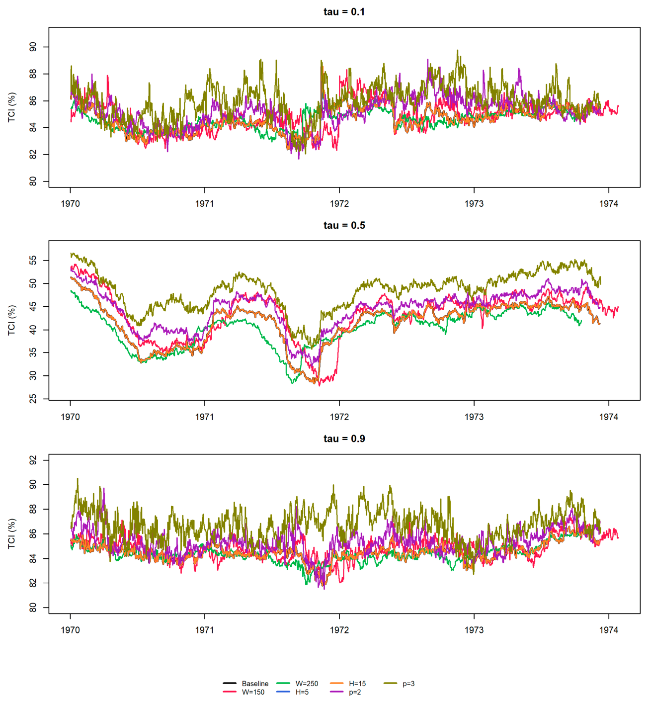
Figure A2.
Dynamic total volatility connectedness parameter sensitivity.
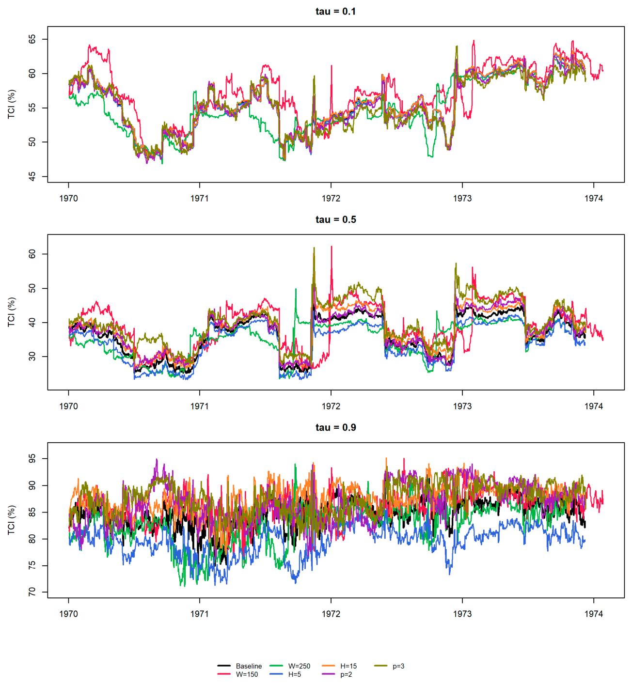
Figure A3.
Dynamic total skewness connectedness parameter sensitivity.
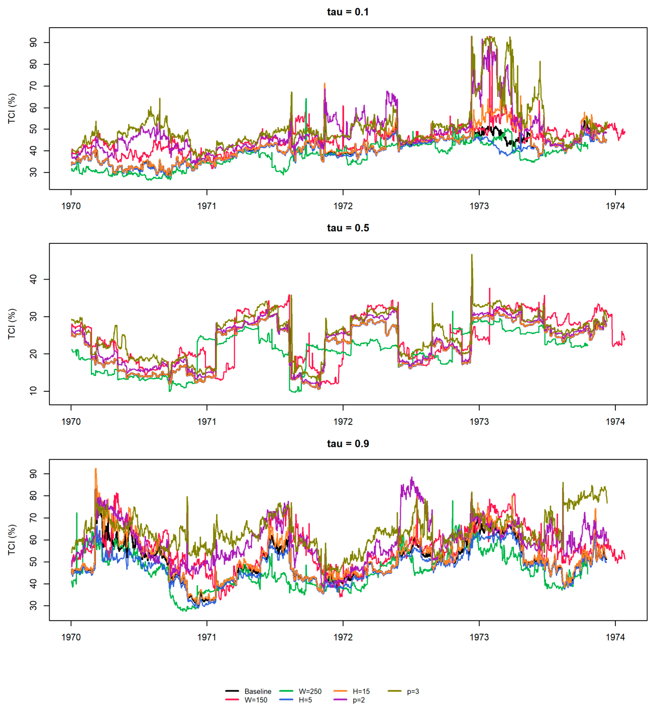
Figure A4.
Dynamic total kurtosis connectedness parameter sensitivity.
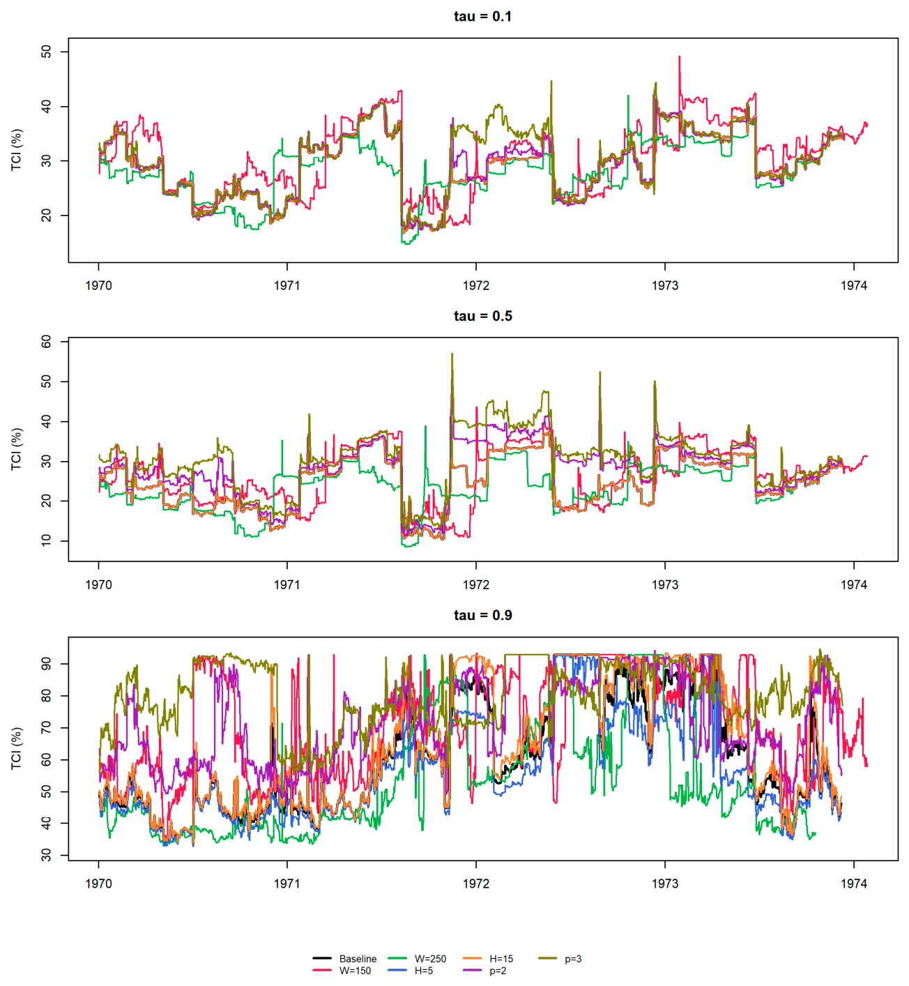
Figure A5.
Robustness of total and net spillovers for return risks.
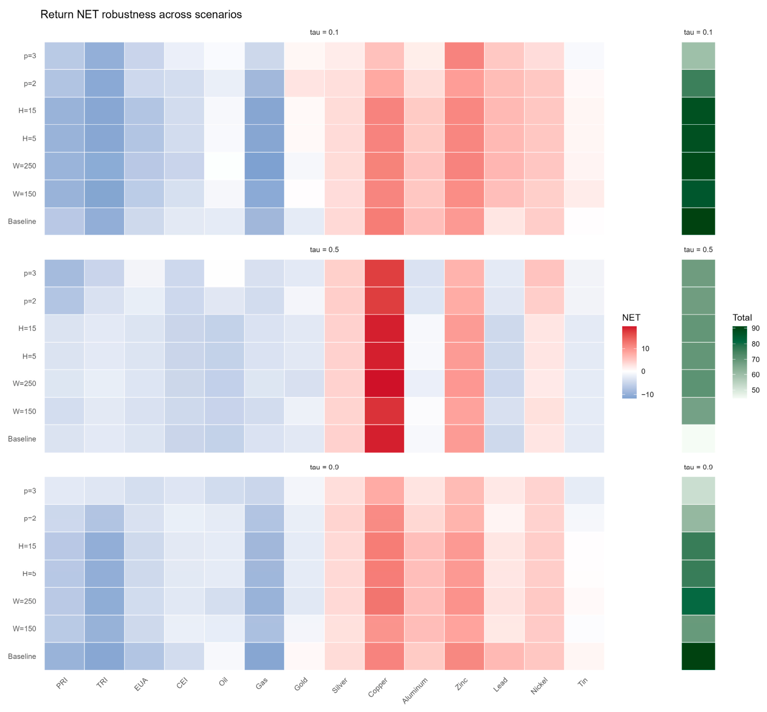
Figure A6.
Robustness of total and net spillovers for volatility risks.
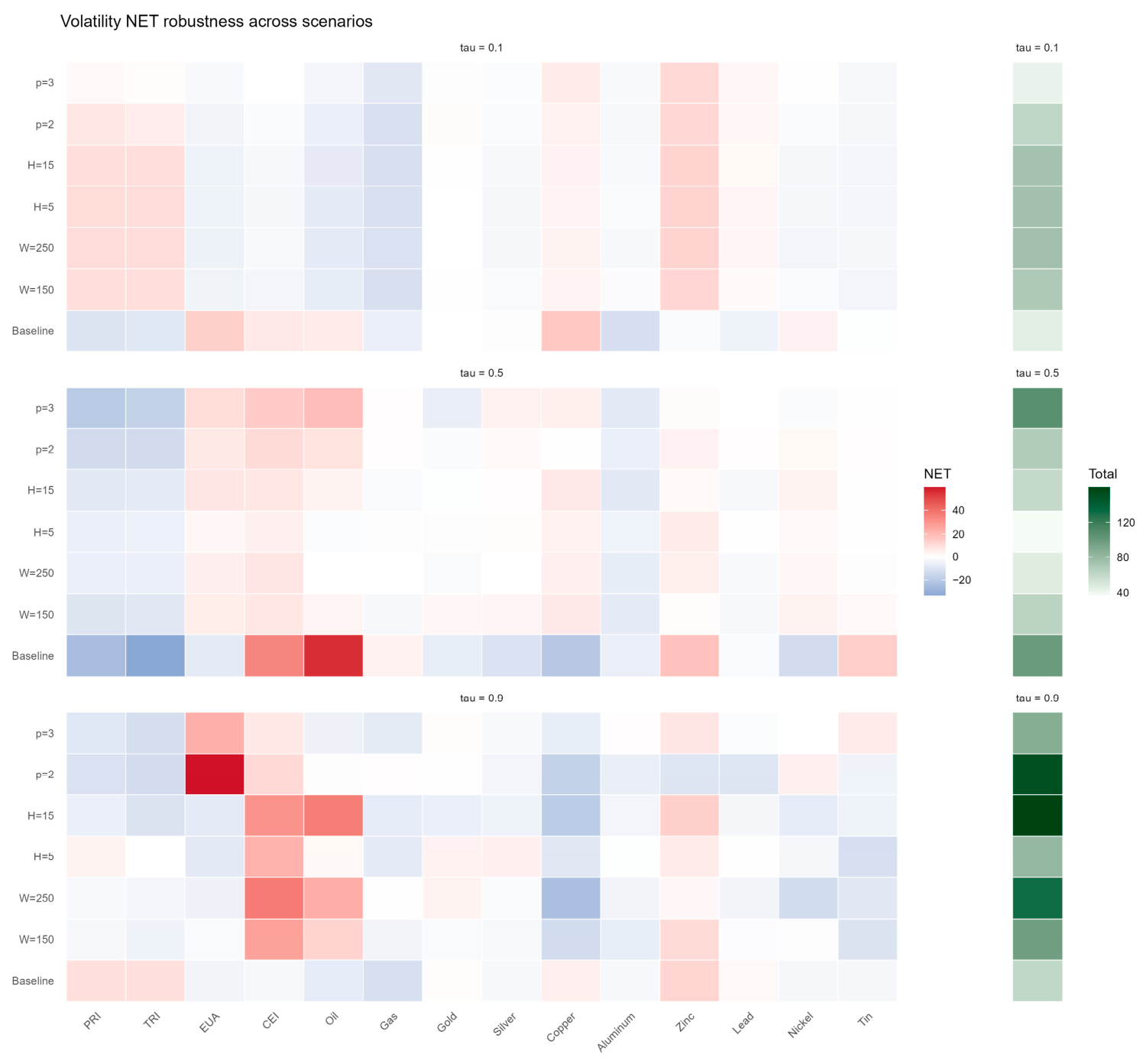
Figure A7.
Robustness of total and net spillovers for skewness risks.
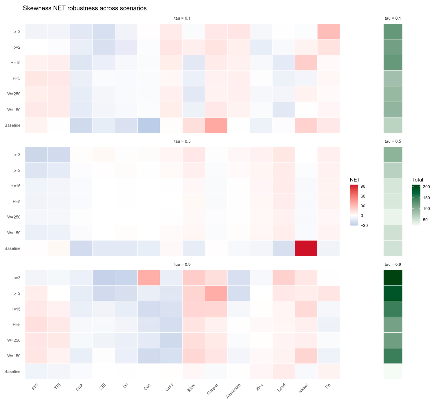
Figure A8.
Robustness of total and net spillovers for kurtosis risks.
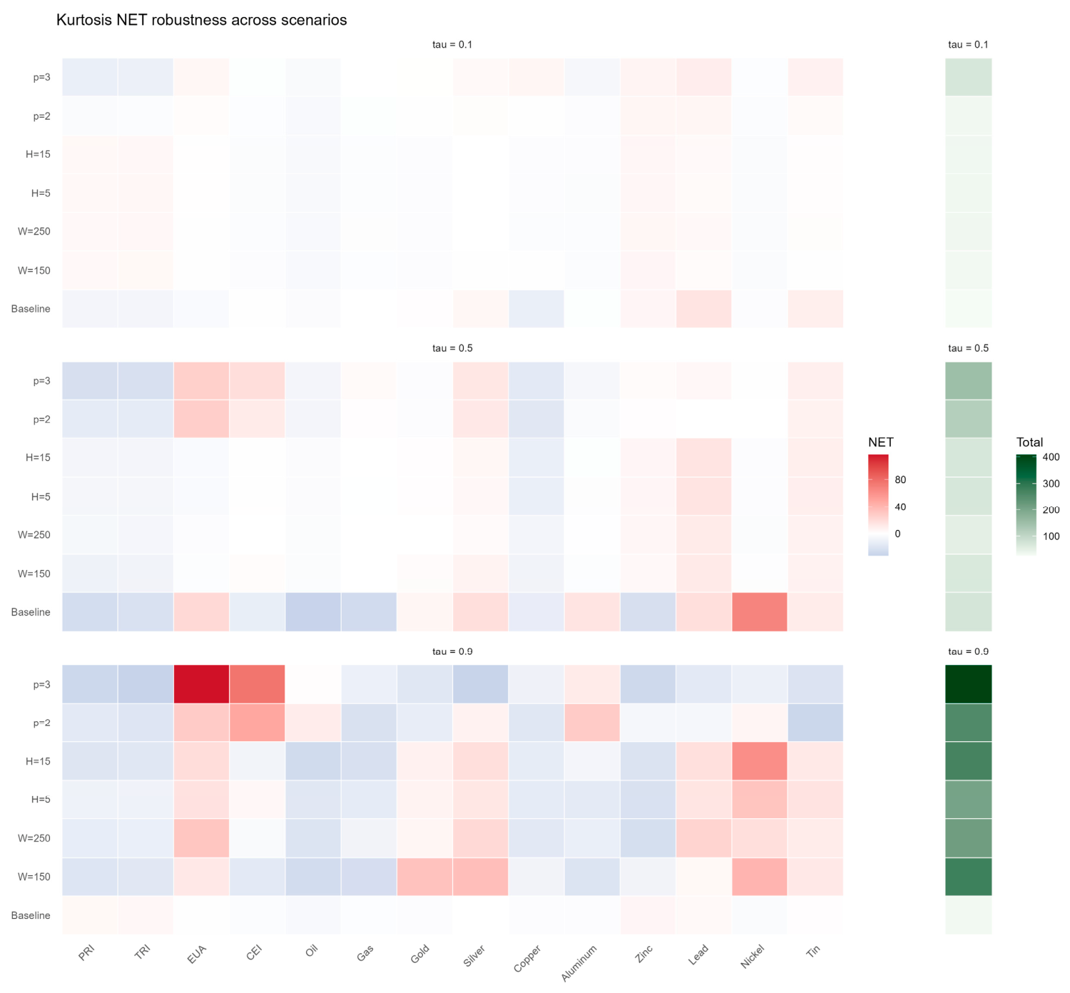
Figure A9.
Total connectedness for return spillovers to the exclusion of extreme observations.
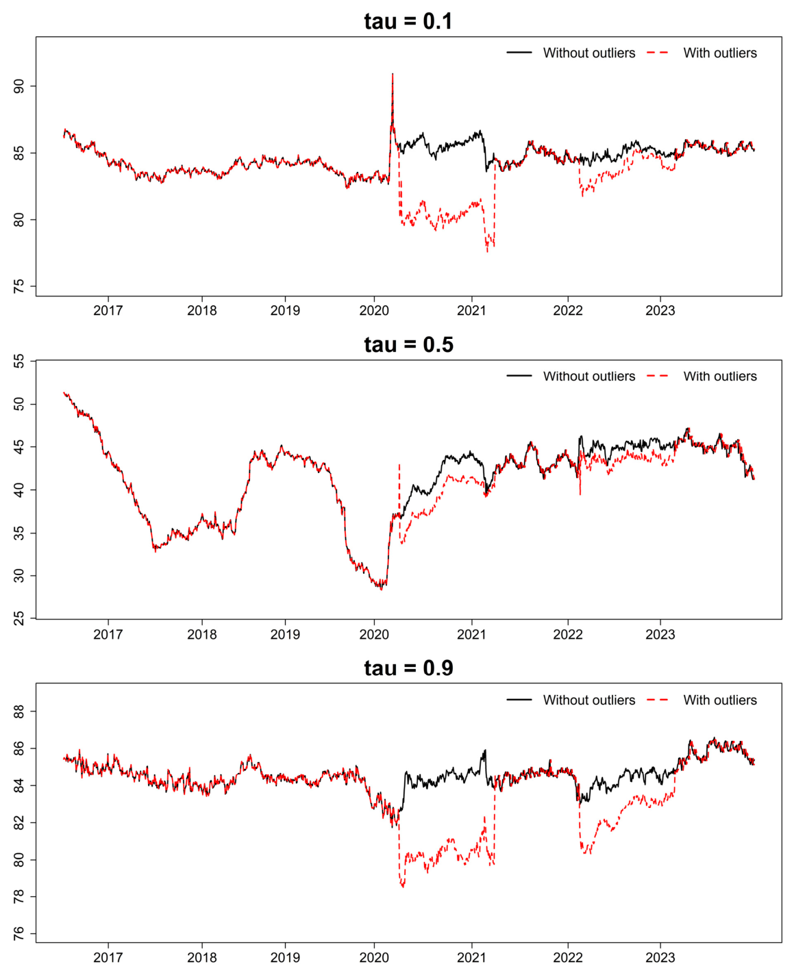
Figure A10.
Total connectedness for volatility spillovers to the exclusion of extreme observations.
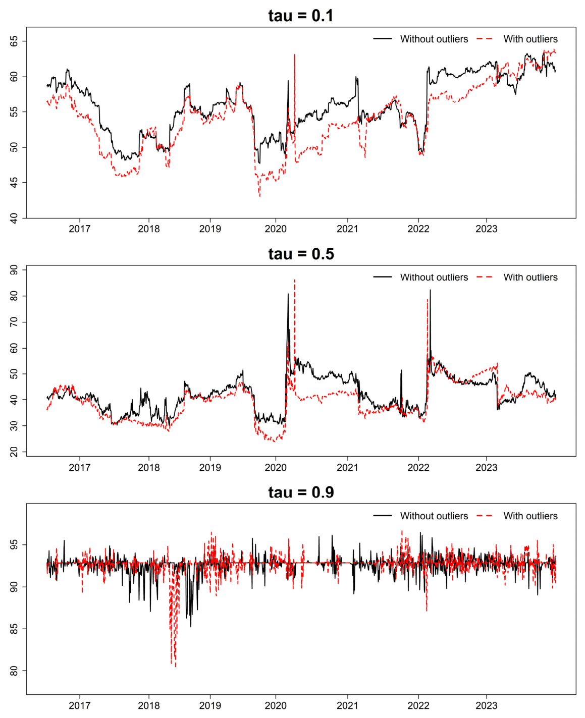
Figure A11.
Total connectedness for skewness spillovers to the exclusion of extreme observations.
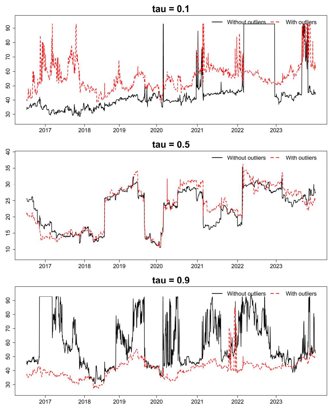
Figure A12.
Total connectedness for kurtosis spillovers to the exclusion of extreme observations.
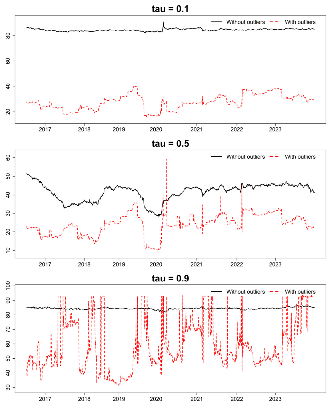
References
- Pacelli, V.; Foglia, M.; Mariano, D. The link between climate and systemic risk: A bibliometric and systematic literature review. Res. Int. Bus. Finance 2025, 79, 103072. [Google Scholar] [CrossRef] [Scilit]
- Adeyemi, F.A.; Jempeji, A.B.A.; Olaniran, A.O.; Taliat, M.K.; Adeleke, A.T. Climate risks and financial stability: A global evidence. Finance Res. Open 2025, 1, 100032. [Google Scholar] [CrossRef] [Scilit]
- Caldecott, B. (Ed.) Stranded Assets and the Environment: Risk, Resilience and Opportunity; Routledge: Abingdon, UK, 2018. [Google Scholar] [CrossRef] [Scilit]
- Rao, A.; Lucey, B.; Kumar, S. Climate Risk and Carbon Emissions: Examining Their Impact on Key Energy Markets through Asymmetric Spillovers. Energy Econ. 2023, 126, 106970. [Google Scholar] [CrossRef] [Scilit]
- Reboredo, J.C.; Ugolini, A. Climate transition risk, profitability and stock prices. Int. Rev. Financ. Anal. 2022, 83, 102271. [Google Scholar] [CrossRef] [Scilit]
- Mansoux, J.; Soler, T. Carbon data isn’t the whole story: A price signal approach to measure climate transition risk and improve asset pricing. J. Clim. Finance 2024, 7, 100042. [Google Scholar] [CrossRef] [Scilit]
- Zhou, Y.; Wu, S.; Liu, Z.; Rognone, L. The asymmetric effects of climate risk on higher-moment connectedness among carbon, energy and metals markets. Nat. Commun. 2023, 14, 7157. [Google Scholar] [CrossRef] [Scilit] [PubMed]
- Hoque, M.E.; Soo-Wah, L.; Bilgili, F.; Ali, H. Connectedness and Spillover Effects of US Climate Policy Uncertainty on Energy Stock, Alternative Energy Stock, and Carbon Future. Environ. Sci. Pollut. Res. 2022, 30, 18956–18972. [Google Scholar] [CrossRef] [Scilit] [PubMed]
- Su, C.-W.; Yuan, X.; Tao, R.; Shao, X. Time and frequency domain connectedness analysis of the energy transformation under climate policy. Technol. Forecast. Soc. 2022, 184, 121978. [Google Scholar] [CrossRef] [Scilit]
- Adeabah, D.; Pham, T.P. Asymmetric tail risk spillover and co-movement between climate risk and the international energy market. Energy Econ. 2025, 141, 108122. [Google Scholar] [CrossRef] [Scilit]
- Banerjee, A.K.; Boubaker, S.; Al-Nassar, N.S. Climate policy initiatives, green finance, and carbon risk interconnectedness. Finance Res. Lett. 2024, 67, 105776. [Google Scholar] [CrossRef] [Scilit]
- Pham, L.; Kamal, J.B. Blessings or curse: How do media climate change concerns affect commodity tail risk spillovers? J. Commod. Mark. 2024, 34, 100407. [Google Scholar] [CrossRef] [Scilit]
- Ouyang, H.; Huang, X.; Yu, B. Risk spillover effects of climate uncertainty on commodity markets: From the dual perspective of physical risk and transition risk. Int. Rev. Financ. Anal. 2025, 105, 104390. [Google Scholar] [CrossRef] [Scilit]
- Lemoine, D.; Traeger, C.P. Economics of tipping the climate dominoes. Nat. Clim. Change 2016, 6, 514–519. [Google Scholar] [CrossRef] [Scilit]
- Sanin, M.E.; Violante, F.; Mansanet-Bataller, M. Understanding volatility dynamics in the EU-ETS market. Energy Policy 2015, 82, 321–331. [Google Scholar] [CrossRef] [Scilit]
- Bonato, M.; Cepni, O.; Gupta, R.; Pierdzioch, C. Climate risks and realized volatility of major commodity currency exchange rates. J. Financ. Mark. 2023, 62, 100760. [Google Scholar] [CrossRef] [Scilit]
- Wang, K.-H.; Kan, J.-M.; Qiu, L.; Xu, S. Climate policy uncertainty, oil price and agricultural commodity: From quantile and time perspective. Econ. Anal. Policy 2023, 78, 256–272. [Google Scholar] [CrossRef] [Scilit]
- Guo, J.; Long, S.; Luo, W. Nonlinear effects of climate policy uncertainty and financial speculation on the global prices of oil and gas. Int. Rev. Financ. Anal. 2022, 83, 102286. [Google Scholar] [CrossRef] [Scilit]
- Diaz-Rainey, I.; Gehricke, S.A.; Roberts, H.; Zhang, R. Trump vs Paris: The impact of climate policy on US listed oil and gas firm returns and volatility. Int. Rev. Financ. Anal. 2021, 76, 101746. [Google Scholar] [CrossRef] [Scilit]
- Lee, C.C.; Yuan, Z.; Lee, C.C.; Chang, Y.F. The impact of renewable energy technology innovation on energy poverty: Does climate risk matter? Energy Econ. 2022, 116, 106427. [Google Scholar] [CrossRef] [Scilit]
- Hao, L.; Kou, X.; Xu, G.; Qiu, X.; Liu, H. Which Emission Reduction Mode Is the Best under the Carbon Cap-and-Trade Mechanism? J. Clean. Prod. 2021, 314, 128053. [Google Scholar] [CrossRef] [Scilit]
- Xie, L.; Zhou, Z.; Hui, S. Does Environmental Regulation Improve the Structure of Power Generation Technology? Evidence from China’s Pilot Policy on the Carbon Emissions Trading Market (CETM). Technol. Forecast. Soc. Change 2022, 176, 121428. [Google Scholar] [CrossRef] [Scilit]
- Song, H.L.; Wang, C.; Zuo, L.S. Review and prospects of the availability constraints of critical byproduct metals for clean energy technologies in the context of carbon neutrality goal. China Popul. Resour. Environ. 2022, 32, 38–48. [Google Scholar] [CrossRef]
- Tost, M.; Hitch, M.; Lutter, S.; Feiel, S.; Moser, P. Carbon prices for meeting the Paris agreement and their impact on key metals. Extr. Ind. Soc. 2020, 7, 593–599. [Google Scholar] [CrossRef] [Scilit]
- Khalfaoui, R.; Medteh-Wali, S.; Viviani, J.-L.; Ben Jabeur, S.; Abedin, M.Z.; Lucey, B.M. How do climate risk and clean energy spillovers, and uncertainty affect U.S. stock markets. Technol. Forecast. Soc. 2022, 185, 122083. [Google Scholar] [CrossRef] [Scilit]
- Cui, J.; Maghyereh, A. Examining perceived spillovers among climate risk, fossil fuel, renewable energy, and carbon markets: A higher-order moment and quantile analysis. J. Commod. Mark. 2025, 38, 100470. [Google Scholar] [CrossRef] [Scilit]
- Liu, C.; Ma, S.; Lu, S.; Zhi, J.; Shen, J.; Li, X.; Shi, C. Study on the time-frequency risk spillover network of “carbon-energy-stock” system under climate risk shock. Energy 2025, 334, 137441. [Google Scholar] [CrossRef] [Scilit]
- Qiao, S.; Chang, Y.; Mai, X.X.; Dang, Y.J. Climate policy uncertainty, clean energy and energy metals: A quantile time-frequency spillover study. Energy Econ. 2024, 139, 107919. [Google Scholar] [CrossRef] [Scilit]
- Adekoya, O.B.; Oliyide, J.A.; Noman, A. The volatility connectedness of the EU carbon market with commodity and financial markets in time- and frequency-domain: The role of the U.S. economic policy uncertainty. Resour. Policy 2021, 74, 102252. [Google Scholar] [CrossRef] [Scilit]
- Jiang, W.; Chen, Y. The time-frequency connectedness among metal, energy and carbon markets pre and during COVID-19 outbreak. Resour. Policy 2022, 77, 102763. [Google Scholar] [CrossRef] [Scilit] [PubMed]
- Ren, Y.; Wang, N.; Zhu, H. Dynamic connectedness of climate risks, oil shocks, and China’s energy futures market: Time-frequency evidence from Quantile-on-Quantile regression. N. Am. J. Econ. Finance 2025, 75, 102263. [Google Scholar] [CrossRef] [Scilit]
- Yao, Z.; Chen, Y.; Deng, S.; Zhang, Y.; Wei, Y. Carbon emission allowance, global climate risk, and agricultural futures: An extreme spillover analysis in China. Finance Res. Lett. 2025, 71, 106391. [Google Scholar] [CrossRef] [Scilit]
- Nekhili, R.; Bouri, E. Higher-order moments and co-moments’ contribution to spillover analysis and portfolio risk management. Energy Econ. 2023, 119, 106596. [Google Scholar] [CrossRef] [Scilit]
- Wang, Y.; Cheung, A.W.K.; Yan, W.L.; Wang, B. Connectedness of China’s green bond and green stock markets at the low- and high-order moments: The role of economic and climate policy uncertainty. N. Am. J. Econ. Finance 2025, 78, 102410. [Google Scholar] [CrossRef] [Scilit]
- Chu, W.-J.; Fan, L.-W.; Zhou, P. Extreme spillovers across carbon and energy markets: A multiscale higher-order moment analysis. Energy Econ. 2024, 138, 107833. [Google Scholar] [CrossRef] [Scilit]
- Katz, D.J.; Ramirez, M.E. Moments of autocorrelation demerit factors of binary sequences. Des. Codes Cryptogr. 2025, 93, 1021–1065. [Google Scholar] [CrossRef] [Scilit]
- Zhu, P.; Tang, Y.; Wei, Y.; Lu, T. Multidimensional risk spillovers among crude oil, the US and Chinese stock markets: Evidence during the COVID-19 epidemic. Energy 2021, 231, 120949. [Google Scholar] [CrossRef] [Scilit] [PubMed]
- Yang, C.; Lei, X.; Shi, B. Spillovers among China’s precious and industrial metals markets: Evidence from higher moments and jumps. Trans. Nonferrous Met. Soc. China 2022, 32, 1362–1384. [Google Scholar] [CrossRef] [Scilit]
- Gao, W.; Yang, S. Higher-order moments spillovers among energy, carbon and tourism markets: Time- and frequency-domain evidence. PLoS ONE 2024, 19, e0313002. [Google Scholar] [CrossRef] [Scilit] [PubMed]
- Wu, H.; Huang, Y. Identifying Risk Transmission in Carbon, Energy and Metal Markets: Evidence from a Novel Quantile Frequency Connectedness Approach. N. Am. J. Econ. Finance 2025, 76, 102354. [Google Scholar] [CrossRef] [Scilit]
- Wu, G.; Hu, G. Asymmetric spillovers and resilience in physical and financial assets amid climate policy uncertainties: Evidence from China. Technol. Forecast. Soc. 2024, 208, 123701. [Google Scholar] [CrossRef] [Scilit]
- Khalfaoui, R.; Stef, N.; Arfi, W.B.; Ben Jabeur, S. Dynamic spillover effects and connectedness among climate change, technological innovation, and uncertainty: Evidence from a quantile VAR network and wavelet coherence. Technol. Forecast. Soc. 2022, 181, 121743. [Google Scholar] [CrossRef] [Scilit]
- Foglia, M.; Plakandaras, V.; Gupta, R.; Ji, Q. Long-span multi-layer spillovers between moments of advanced equity markets: The role of climate risks. Res. Int. Bus. Finance 2025, 74, 102667. [Google Scholar] [CrossRef] [Scilit]
- Gong, X.-L.; Zhao, M.; Wu, Z.-C.; Jia, Z.-C.; Jia, K.-W.; Xiong, X. Research on tail risk contagion in international energy markets—The quantile time-frequency volatility spillover perspective. Energy Econ. 2023, 121, 106678. [Google Scholar] [CrossRef] [Scilit]
- Zhu, B.; Deng, Y.; Hu, X. Global energy security: Do internal and external risk spillovers matter? A multilayer network method. Energy Econ. 2023, 126, 106961. [Google Scholar] [CrossRef] [Scilit]
- Ouyang, Z.; Zhou, X.; Wang, G.; Liu, S.; Lu, M. Multilayer networks in the frequency domain: Measuring volatility connectedness among Chinese financial institutions. Int. Rev. Econ. Finance 2024, 92, 909–928. [Google Scholar] [CrossRef] [Scilit]
- Dai, Z.; Tang, R.; Zhang, X. Multilayer network analysis for measuring the inter-connectedness between the oil market and G20 stock markets. Energy Econ. 2023, 120, 106639. [Google Scholar] [CrossRef] [Scilit]
- Banerjee, A.K. Second-order moment risk connectedness across climate and geopolitical risk and global commodity markets. Econ. Lett. 2024, 235, 111551. [Google Scholar] [CrossRef] [Scilit]
- Xu, C.; Chen, Z.; Zhu, W.; Zhi, J.; Yu, Y.; Shi, C. Time-frequency spillover and early warning of climate risk in international energy markets and carbon markets: From the perspective of complex network and machine learning. Energy 2025, 318, 134857. [Google Scholar] [CrossRef] [Scilit]
- Abakah, E.J.A.; Tiwari, A.K.; Lee, C.C.; Ntow-Gyamfi, M. Quantile price convergence and spillover effects among Bitcoin, Fintech, and artificial intelligence stocks. Int. Rev. Finance 2023, 23, 187–205. [Google Scholar] [CrossRef] [Scilit]
- Bua, G.; Kapp, D.; Ramella, F.; Rognone, L. Transition versus physical climate risk pricing in European financial markets: A text-based approach. Eur. J. Finance 2024, 30, 2076–2110. [Google Scholar] [CrossRef] [Scilit]
- Lu, P.; Wang, Z. Frequency connectedness of climate risk and commodity markets: A time-varying quantile framework. J. Clean. Prod. 2025, 524, 146175. [Google Scholar] [CrossRef] [Scilit]
- Zhang, T.; Li, P.F.; Zhou, W.X. Spillover effects between climate policy uncertainty, energy markets, and food markets: A time–frequency analysis. Finance Res. Lett. 2025, 82, 107553. [Google Scholar] [CrossRef] [Scilit]
- Hong, S.; Luo, Y.; Cheng, J. Multidimensional linkages among carbon, energy, and industrial metals markets: Evidence from spillover effects and co-movements. Front. Environ. Sci. 2026, 14, 1738158. [Google Scholar] [CrossRef] [Scilit]
- Chu, W.J.; Fan, L.W.; Zhou, P.; Zhou, X. How do uncertainties drive the risk spillover across China’s carbon, energy, and rare earth markets? J. Environ. Manag. 2026, 399, 128623. [Google Scholar] [CrossRef] [Scilit] [PubMed]
- Diebold, F.X.; Yilmaz, K. Better to give than to receive: Predictive directional measurement of volatility spillovers. Int. J. Forecast. 2012, 28, 57–66. [Google Scholar] [CrossRef] [Scilit]
- Diebold, F.X.; Yılmaz, K. On the network topology of variance decompositions: Measuring the connectedness of financial firms. J. Econom. 2014, 182, 119–134. [Google Scholar] [CrossRef] [Scilit]
- Ando, T.; Greenwood-Nimmo, M.; Shin, Y. Quantile Connectedness: Modeling Tail Behavior in the Topology of Financial Networks. Manag. Sci. 2022, 68, 2401–2431. [Google Scholar] [CrossRef] [Scilit]
- Antonakakis, N.; Chatziantoniou, I.; Gabauer, D. Refined Measures of Dynamic Connectedness based on Time-Varying Parameter Vector Autoregressions. J. Risk Financ. Manag. 2020, 13, 84. [Google Scholar] [CrossRef] [Scilit]
- Baruník, J.; Křehlík, T. Measuring the frequency dynamics of financial connectedness and systemic risk. J. Financ. Econom. 2018, 16, 271–296. [Google Scholar] [CrossRef] [Scilit]
- Mao, X.; Hu, C.; Xiong, L.; Wang, Y. Climate risk attention and financial markets: The time-frequency and quantile perspective. Finance Res. Lett. 2025, 85, 108130. [Google Scholar] [CrossRef] [Scilit]
- Liu, R.; He, L.; Chen, L.; Fu, Y. How climate risks relate to Chinese green finance markets in time-frequency domains? A consideration of extreme market conditions. J. Clean. Prod. 2025, 487, 144596. [Google Scholar] [CrossRef] [Scilit]
- Yang, Y.H.; Shao, Y.H.; Zhou, W.X. Contemporaneous and lagged spillovers between agriculture, crude oil, carbon emission allowance, and climate change. Finance Res. Lett. 2025, 71, 106374. [Google Scholar] [CrossRef] [Scilit]
- Artime, O.; Benigni, B.; Bertagnolli, G.; d’Andrea, V.; Gallotti, R.; Ghavasieh, A.; Raimondo, S.; De Domenico, M. Multilayer Network Science: Theory and Applications: From Cells to Societies; Cambridge University Press: Cambridge, UK, 2021. [Google Scholar] [CrossRef] [Scilit]
- Zhang, Z.; Xu, Y.; Su, F. Climate policy uncertainty and dynamic volatility spillovers in Chinese stock market: Based on sectoral evaluation. J. Manag. Sci. Eng. 2025, 10, 332–347. [Google Scholar] [CrossRef] [Scilit]
- Chen, J.; Liang, Z.; Ding, Q.; Liu, Z. Extreme spillovers among fossil energy, clean energy, and metals markets: Evidence from a quantile-based analysis. Energy Econ. 2022, 107, 105880. [Google Scholar] [CrossRef] [Scilit]
- He, Z.; Qian, W.; Miftah, B.; Abedin, M.Z. Quantile time-frequency spillovers among climate policy uncertainty, energy markets, and stock markets. Int. Rev. Econ. Finance 2025, 103, 104428. [Google Scholar] [CrossRef] [Scilit]
- Zhou, Y.; Wu, S.; Zhang, Z. Multidimensional risk spillovers among carbon, energy and nonferrous metals markets: Evidence from the quantile VAR network. Energy Econ. 2022, 114, 106319. [Google Scholar] [CrossRef] [Scilit]
- Banerjee, A.K.; Özer, Z.S.; Rahman, M.R.; Sensoy, A. How does the time-varying dynamics of spillover between clean and brown energy ETFs change with the intervention of climate risk and climate policy uncertainty? Int. Rev. Econ. Finance 2024, 93, 442–468. [Google Scholar] [CrossRef] [Scilit]
- Deng, J.; Wang, S.; Hou, H.; Zheng, J.; Yin, S.; Chen, G. Asymmetric and heterogeneous impacts of climate policy uncertainty on risk spillovers in China’s traditional energy sector: A tail risk spillover network approach. Sustain. Futures 2025, 10, 100842. [Google Scholar] [CrossRef] [Scilit]
- Jin, Y.; Zhao, H.; Bu, L.; Zhang, D. Geopolitical risk, climate risk and energy markets: A dynamic spillover analysis. Int. Rev. Financ. Anal. 2023, 87, 102597. [Google Scholar] [CrossRef] [Scilit]
- Li, H.; Li, Y.; Guo, L. Extreme risk spillover effect and dynamic linkages between uncertainty and commodity markets: A com-parison between China and America. Resour. Policy 2023, 85, 103839. [Google Scholar] [CrossRef] [Scilit]
- Mao, X.; Wei, P.; Ren, X. Climate Risk and Financial Systems: A Nonlinear Network Connectedness Analysis. J. Environ. Manag. 2023, 340, 117878. [Google Scholar] [CrossRef] [Scilit] [PubMed]
- Wang, K.H.; Wang, Z.S.; Yunis, M.; Kchouri, B. Spillovers and connectedness among climate policy uncertainty, energy, green bond and carbon markets: A global perspective. Energy Econ. 2023, 128, 107170. [Google Scholar] [CrossRef] [Scilit]
- Yan, W.; Cheung, A. The Dynamic Spillover Effects of Climate Policy Uncertainty and Coal Price on Carbon Price: Evidence from China. Finance Res. Lett. 2023, 53, 103400. [Google Scholar] [CrossRef] [Scilit]
- Nakagawa, K.; Uchiyama, Y. GO-GJRSK model with application to higher order risk-based portfolio. Mathematics 2020, 8, 1990. [Google Scholar] [CrossRef] [Scilit]
- Marco, T.; Mighri, Z.; Tiwari, A.K.; Sarwar, S. A Quantile-Time-Frequency Connectedness Investigation through the Dirty and Clean Cryptocurrencies Spillover. J. Clean. Prod. 2023, 425, 138889. [Google Scholar] [CrossRef] [Scilit]
- Chen, J.; Wang, X. Climate policy uncertainty and the Chinese sectoral stock market: A multilayer network analysis. Econ. Syst. 2025, 49, 101250. [Google Scholar] [CrossRef] [Scilit]
- Latora, V.; Marchiori, M. Efficient Behavior of Small-World Networks. Phys. Rev. Lett. 2001, 87, 198701. [Google Scholar] [CrossRef] [Scilit] [PubMed]
- Zhang, Y.-J.; Sun, Y.-F. The Dynamic Volatility Spillover between European Carbon Trading Market and Fossil Energy Market. J. Clean. Prod. 2016, 112, 2654–2663. [Google Scholar] [CrossRef] [Scilit]
- Dickey, D.A.; Fuller, W.A. Likelihood ratio statistics for autoregressive time series with a unit root. Econometrica 1981, 49, 1057–1072. [Google Scholar] [CrossRef] [Scilit]
- Jarque, C.M.; Bera, A.K. Efficient tests for normality, homoscedasticity and serial independence of regression residuals. Econ. Lett. 1980, 6, 255–259. [Google Scholar] [CrossRef] [Scilit]
- Shah, A.A.; Paul, M.; Bhanja, N.; Dar, A.B. Dynamics of connectedness across crude oil, precious metals and exchange rate: Evidence from time and frequency domains. Resour. Policy 2021, 73, 102154. [Google Scholar] [CrossRef] [Scilit]
- Siddique, M.A.; Nobanee, H.; Hasan, M.B.; Uddin, G.S.; Hossain, M.N.; Park, D. How do energy markets react to climate policy uncertainty? Fossil vs. renewable and low-carbon energy assets. Energy Econ. 2023, 128, 107195. [Google Scholar] [CrossRef] [Scilit]
- Hirshleifer, D.; Shumway, T. Good Day Sunshine: Stock Returns and the Weather. J. Finance 2003, 58, 1009–1032. [Google Scholar] [CrossRef] [Scilit]
- Brown, G.W.; Cliff, M.T. Investor sentiment and the near-term stock market. J. Empir. Finance 2004, 11, 1–27. [Google Scholar] [CrossRef] [Scilit]
- Liu, P.; Huang, W. Modelling international sovereign risk information spillovers: A multilayer network approach. N. Am. J. Econ. Finance 2022, 63, 101794. [Google Scholar] [CrossRef] [Scilit]
- Bali, T.G.; Cakici, N. Idiosyncratic Volatility and the Cross Section of Expected Returns. J. Financ. Quant. Anal. 2008, 43, 29–58. [Google Scholar] [CrossRef] [Scilit]
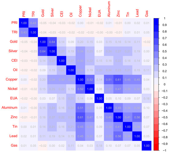
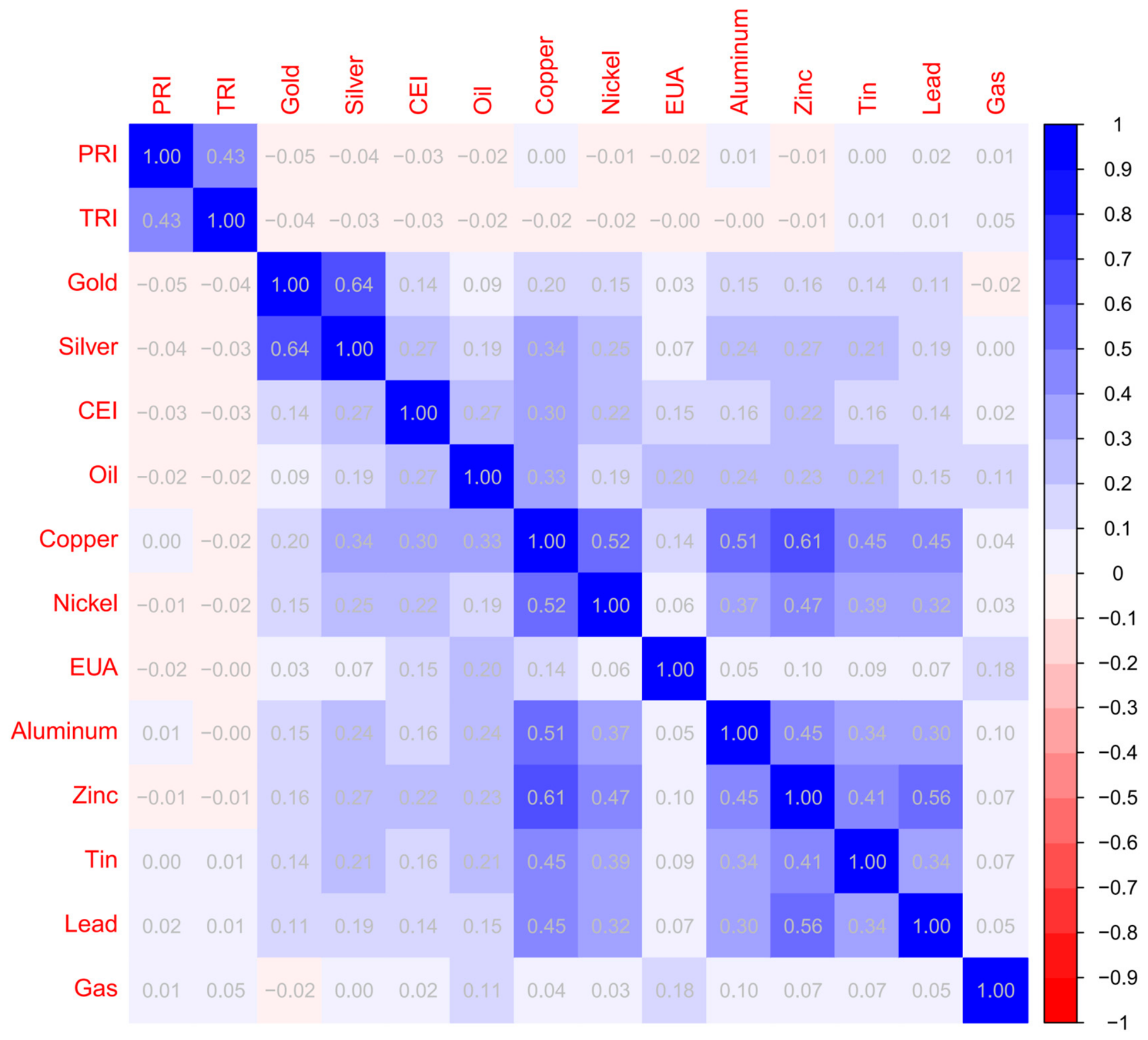
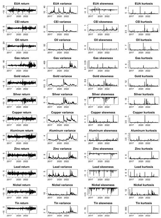
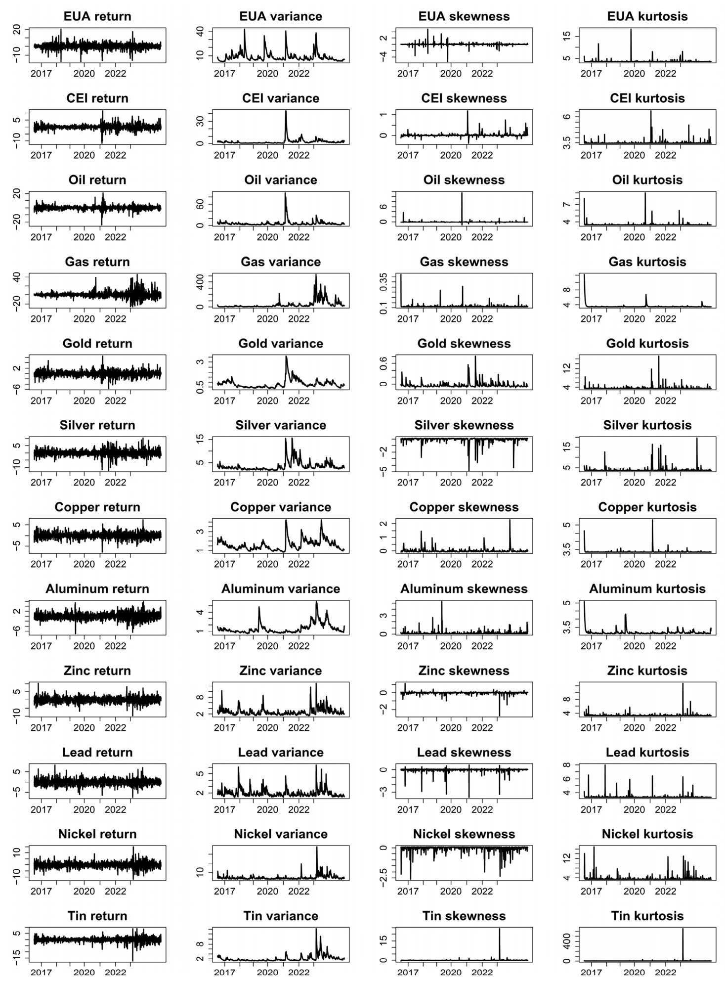
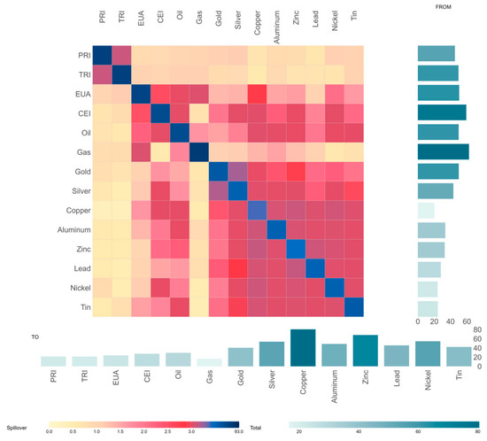
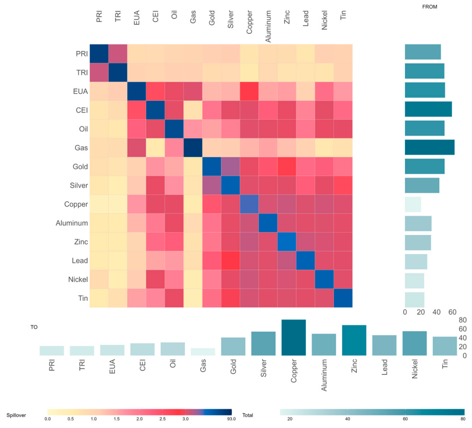
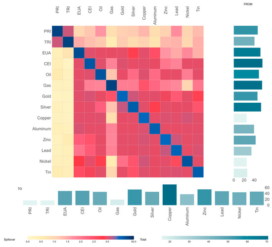
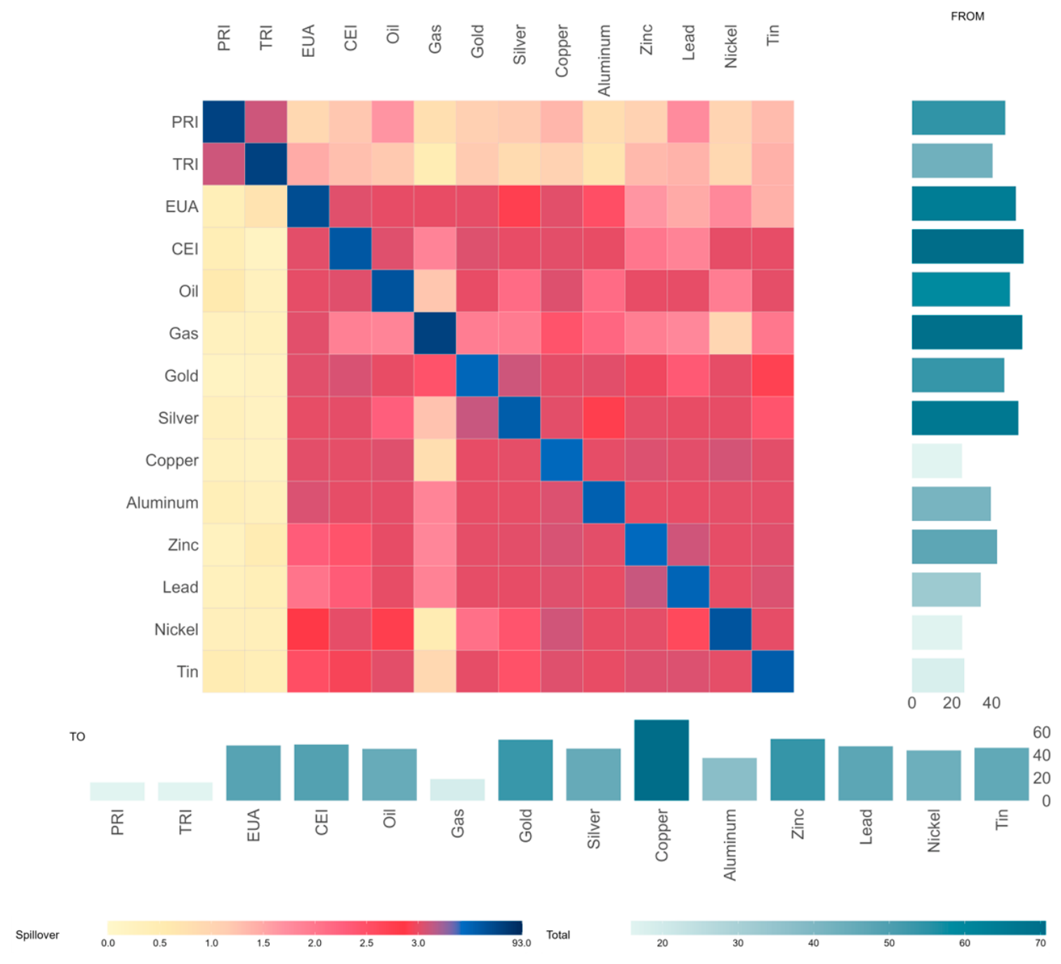
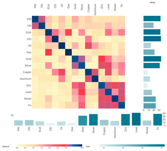
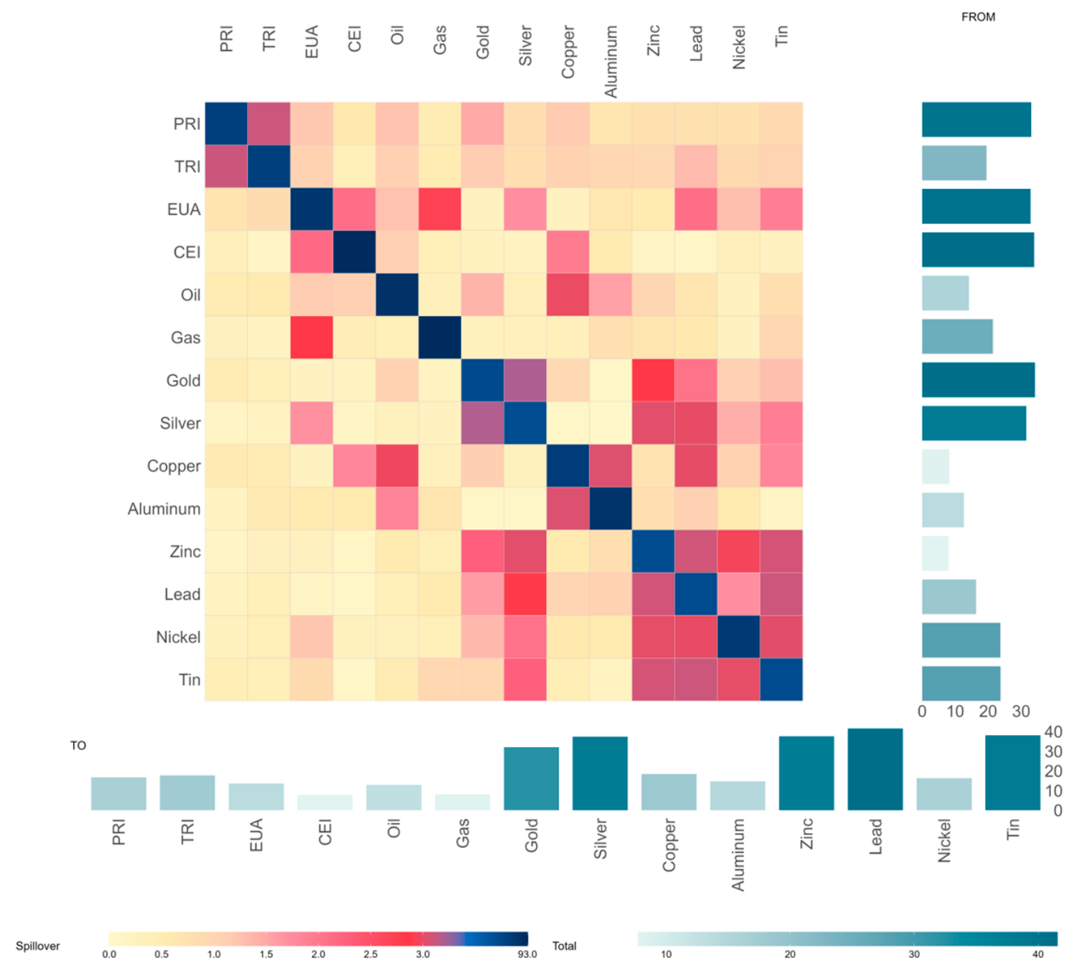
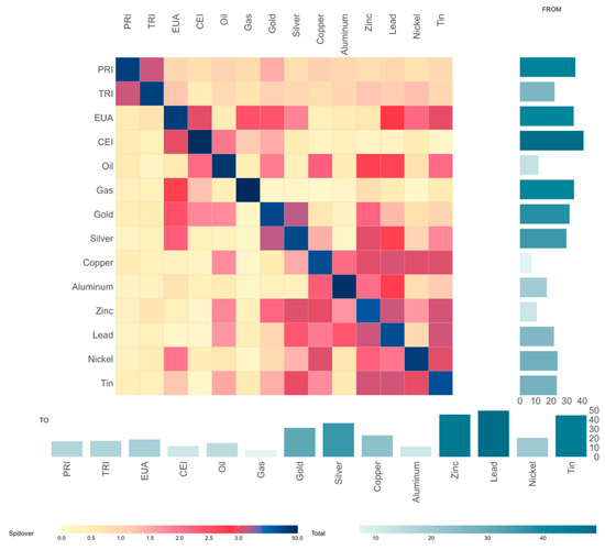
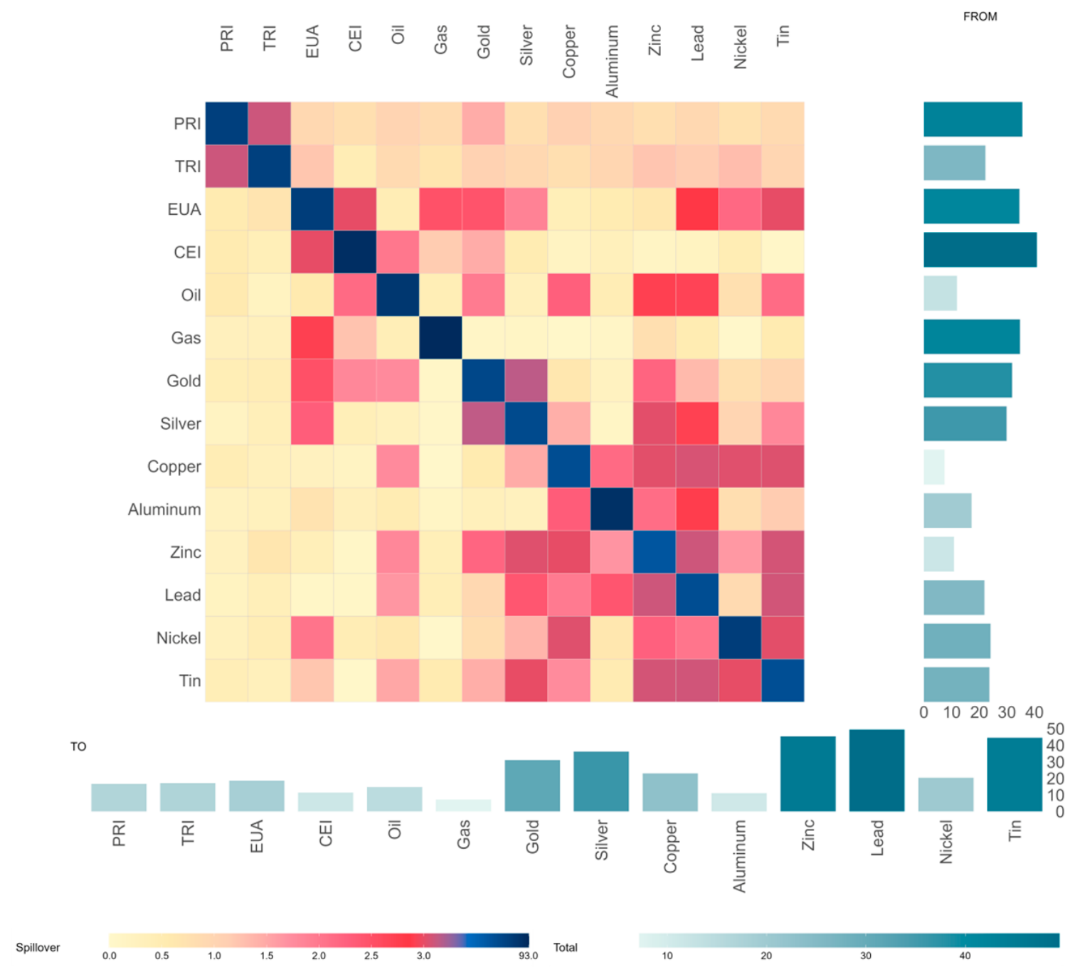
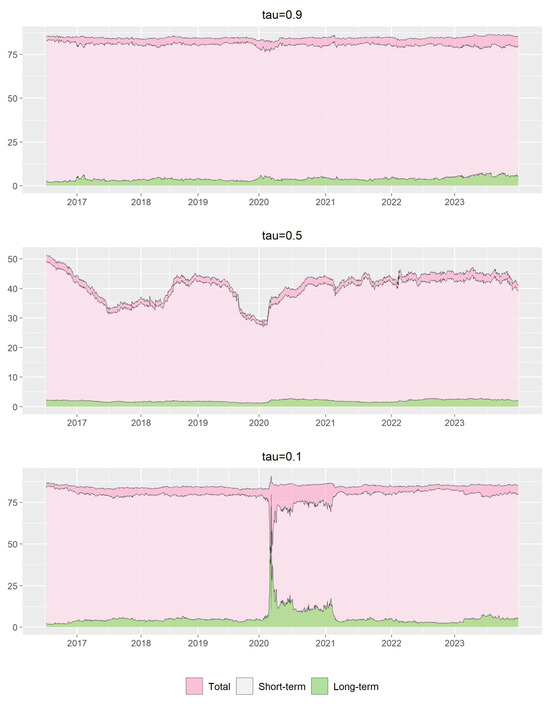
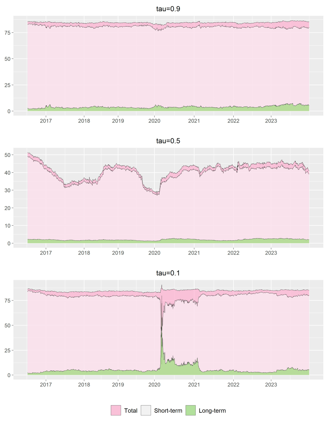
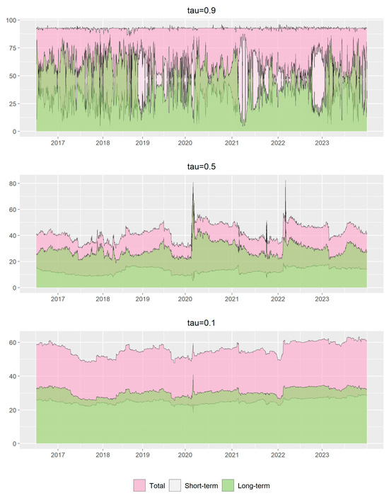
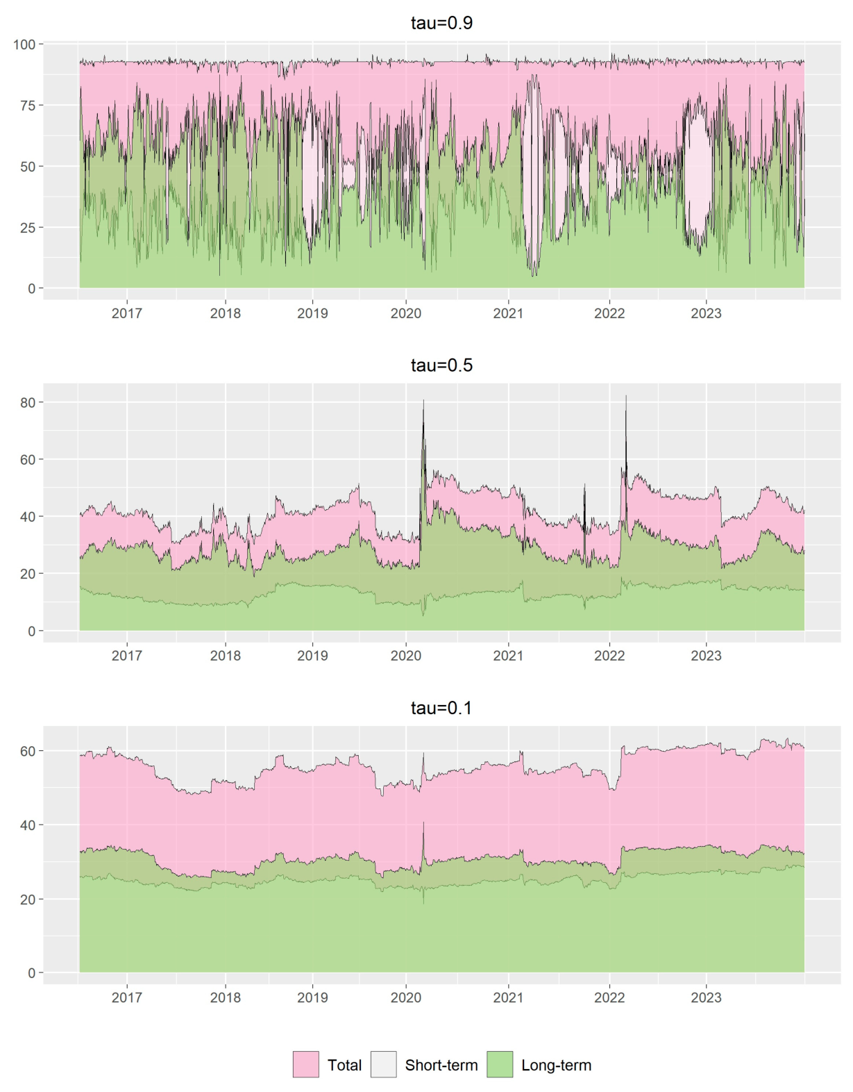
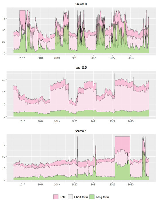
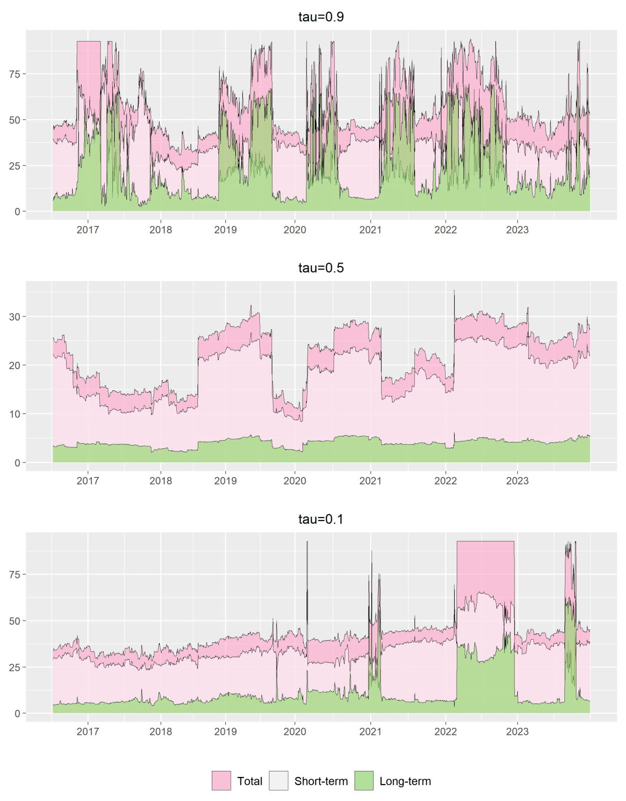
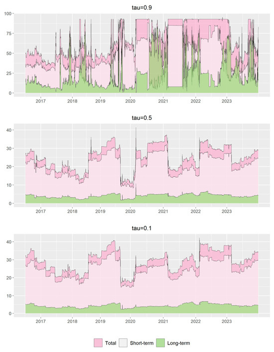
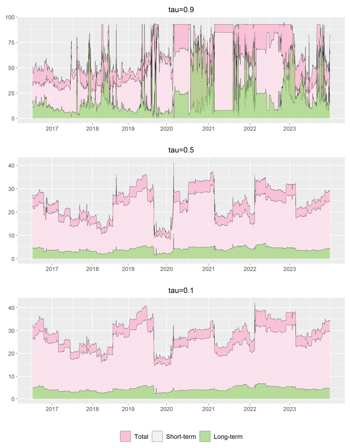
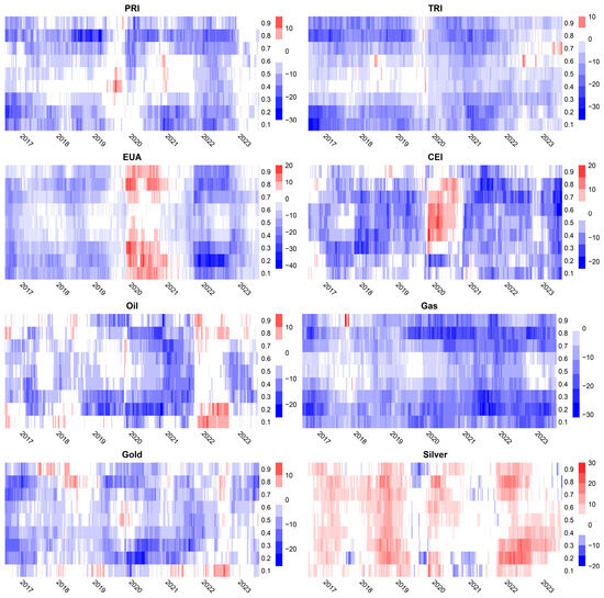
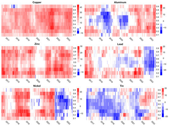
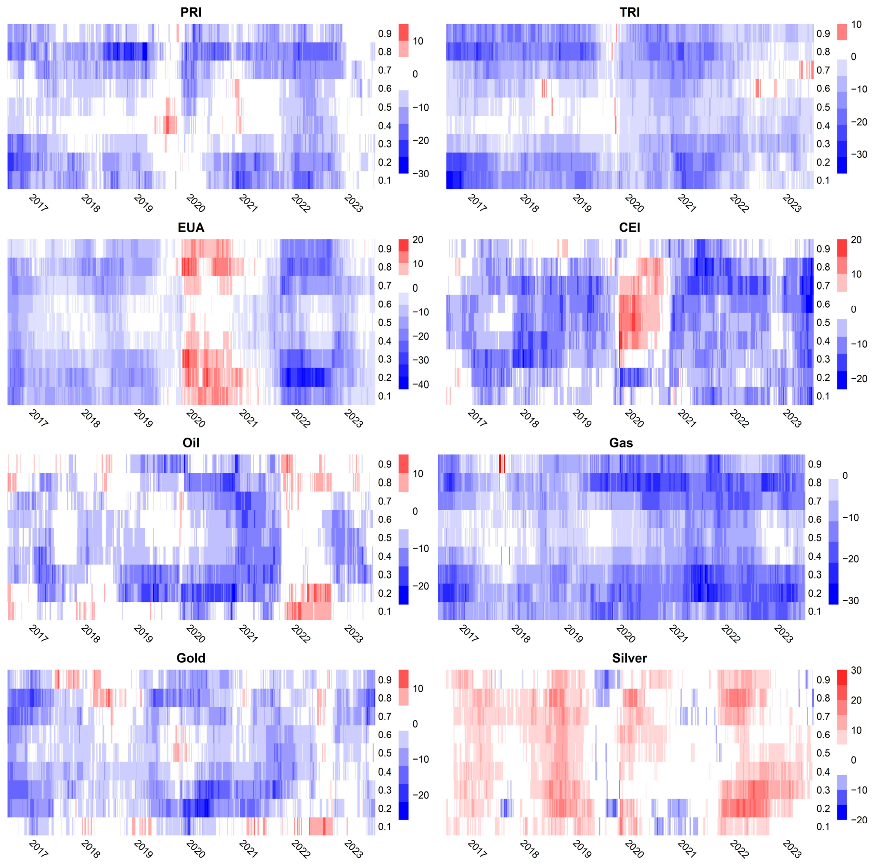
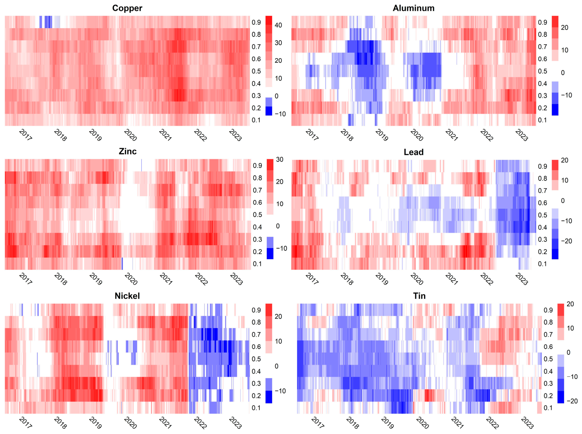
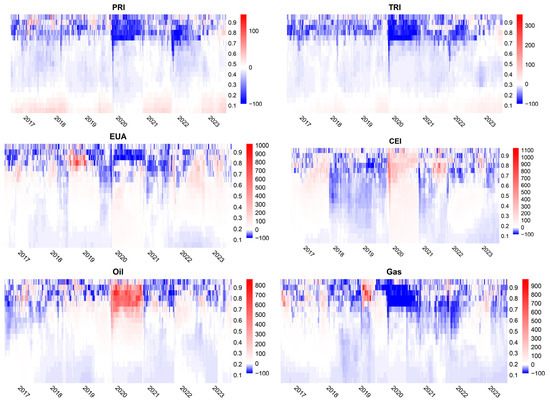
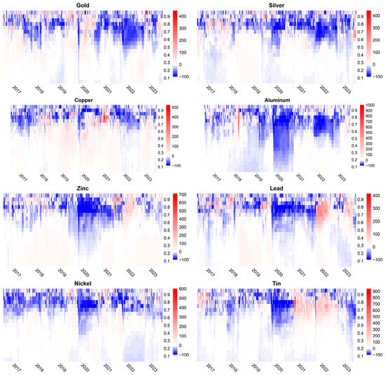
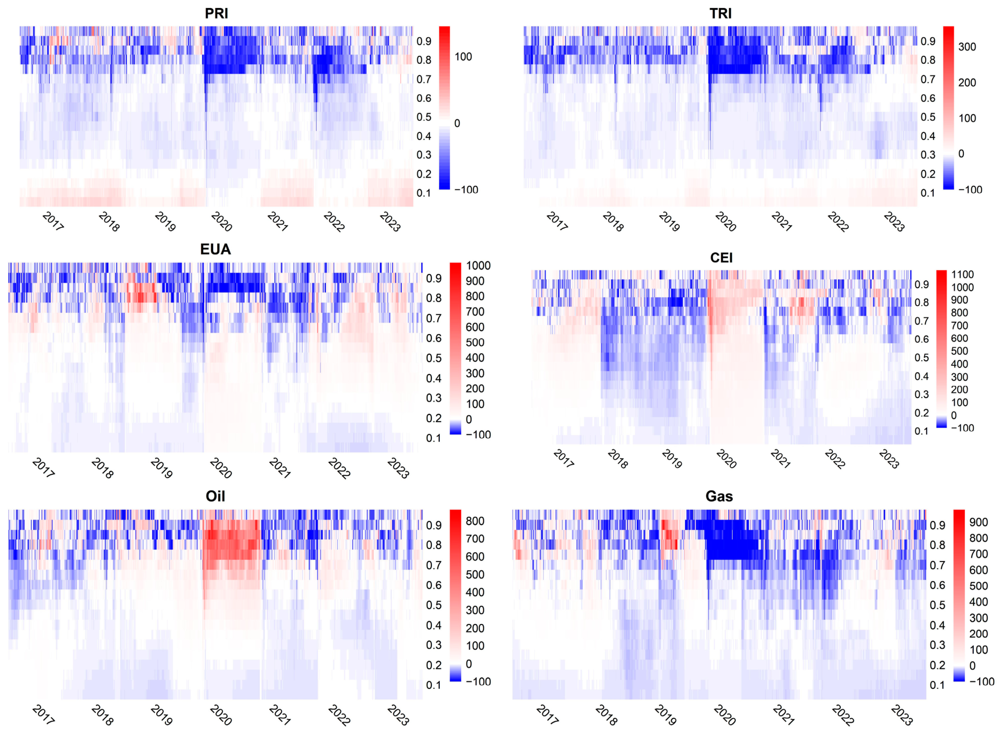
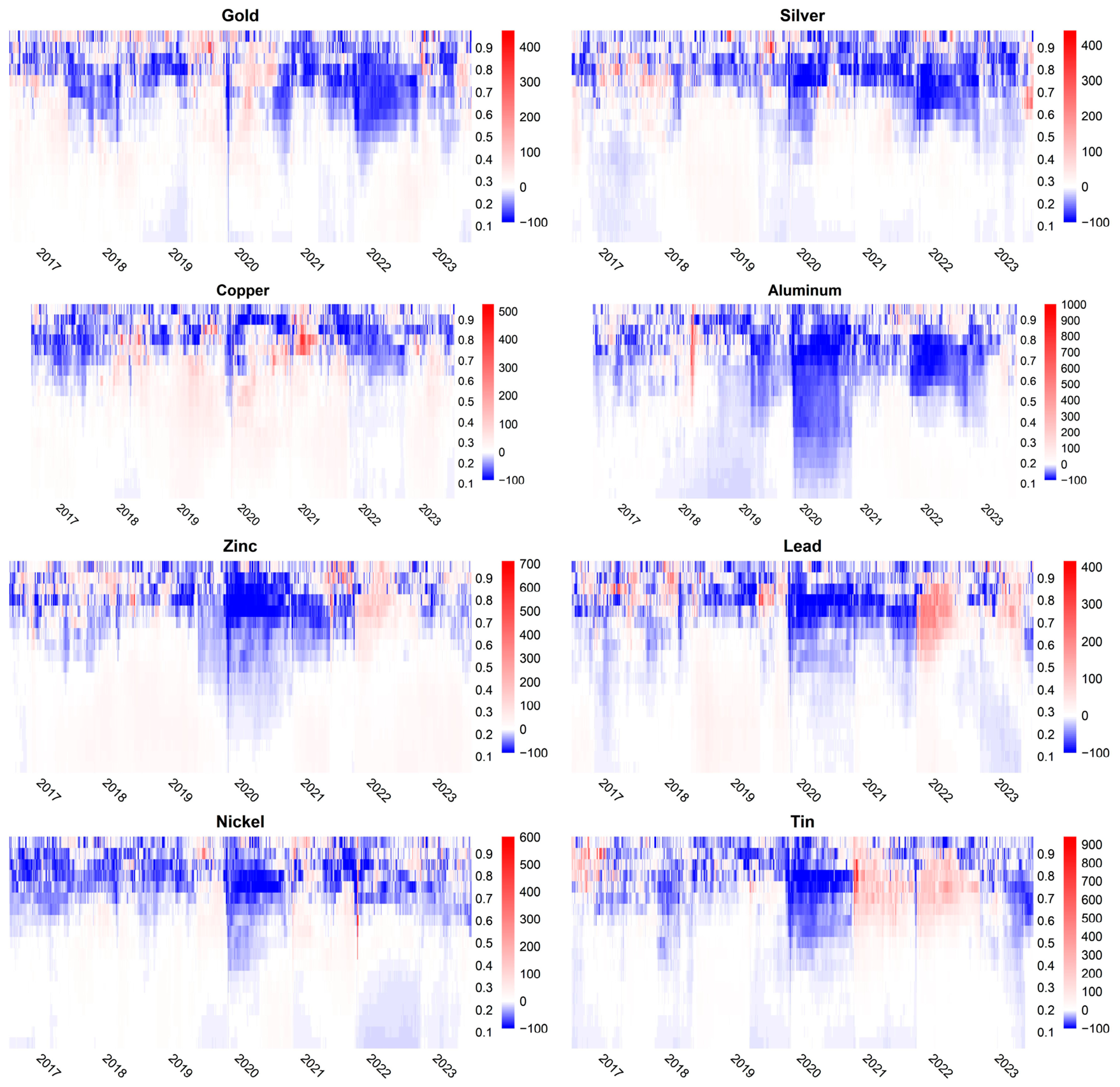
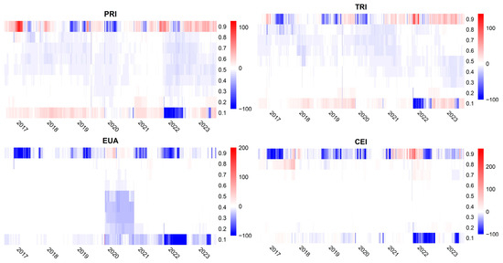
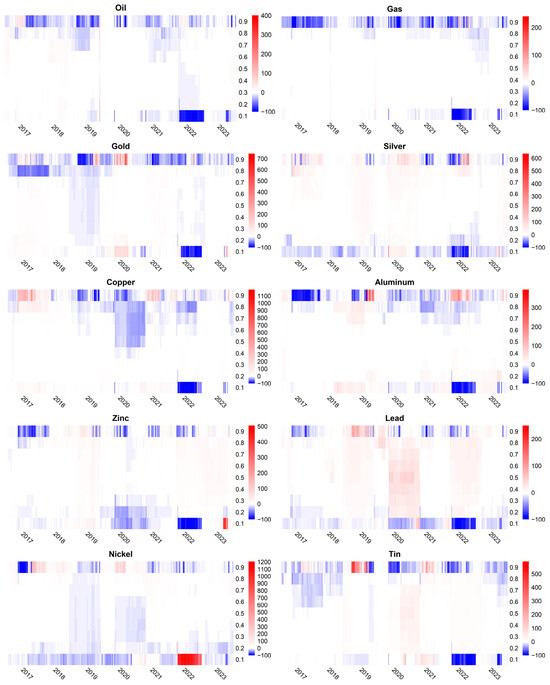
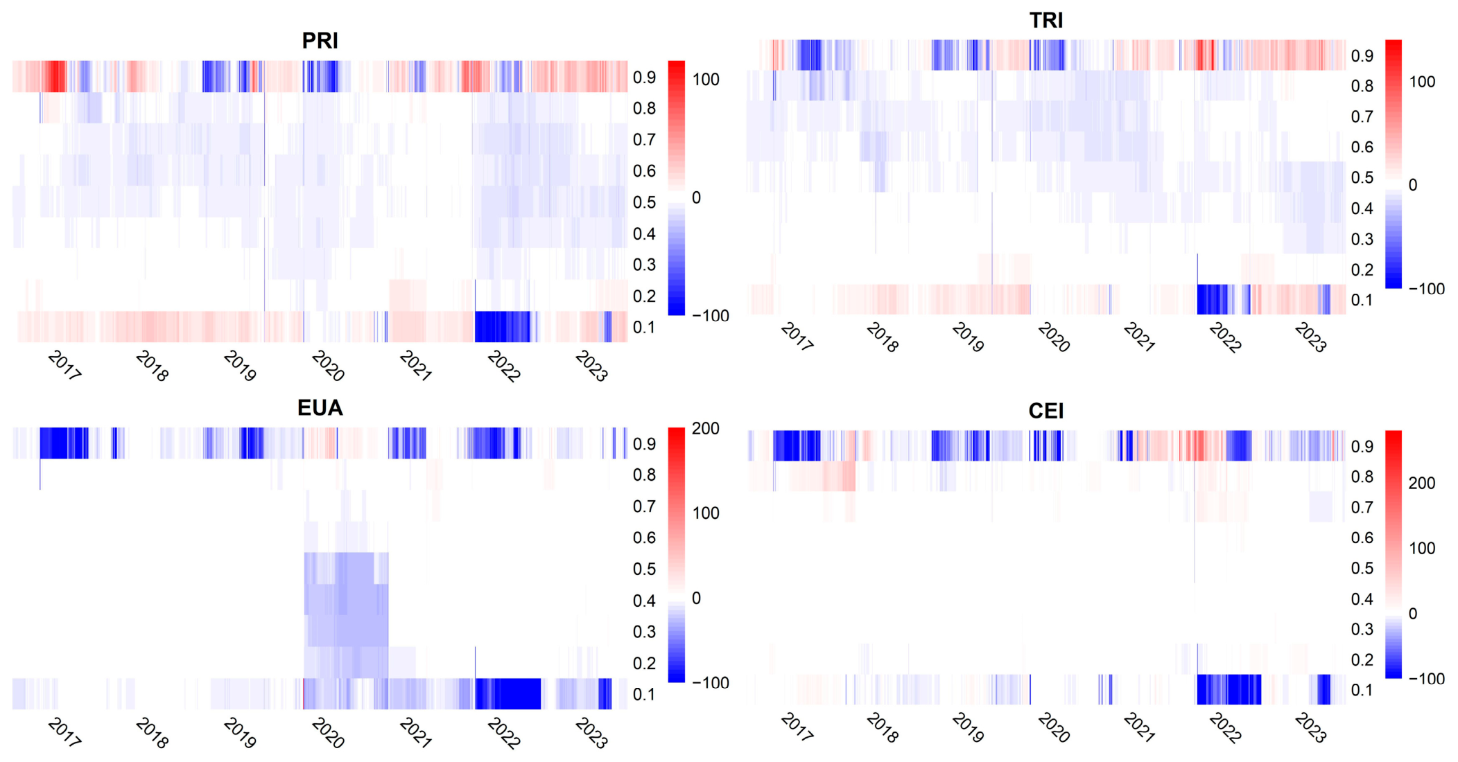
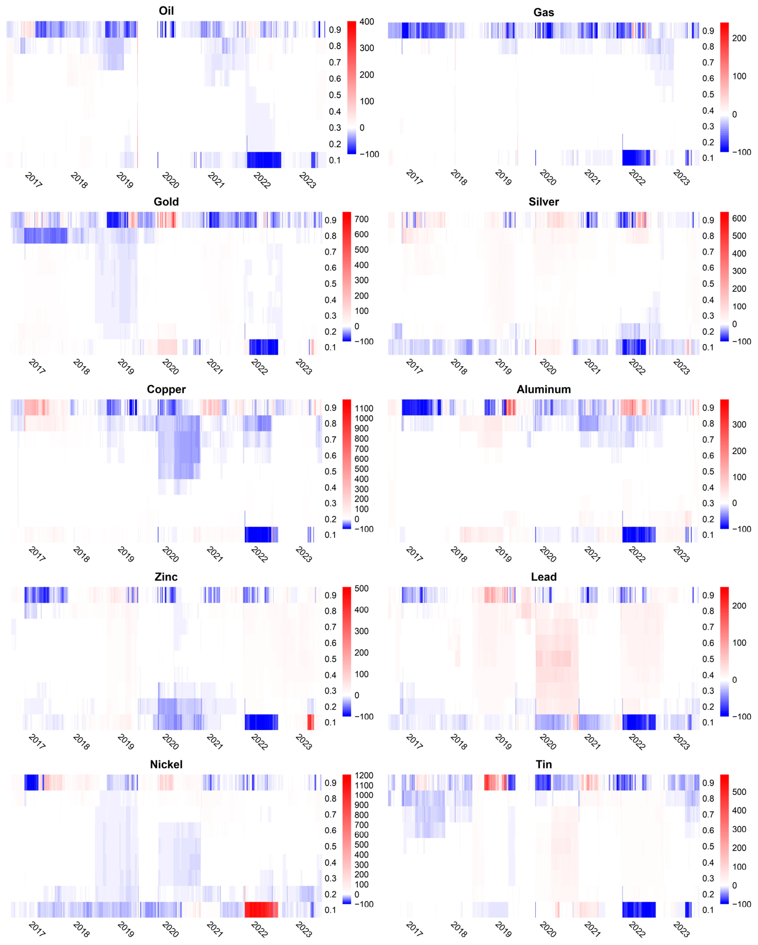
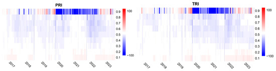
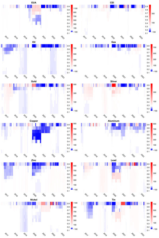
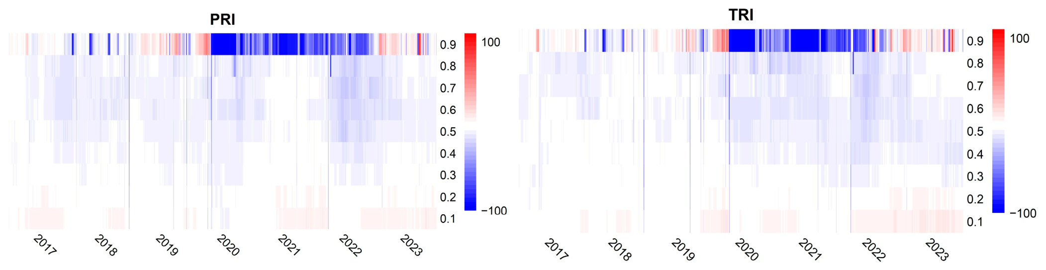
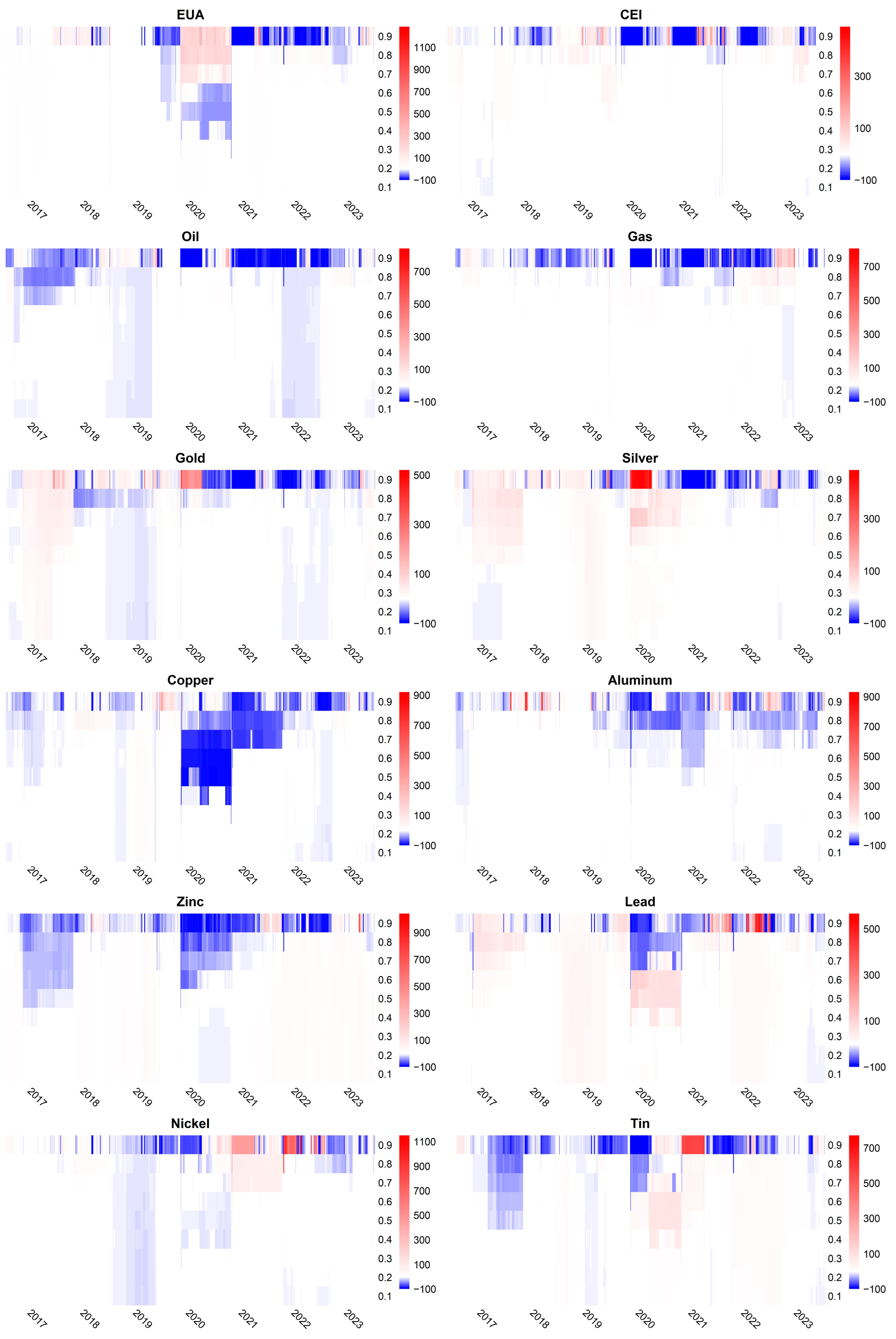
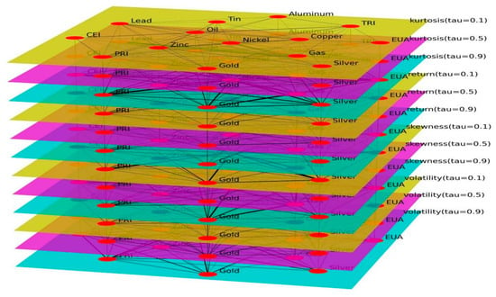
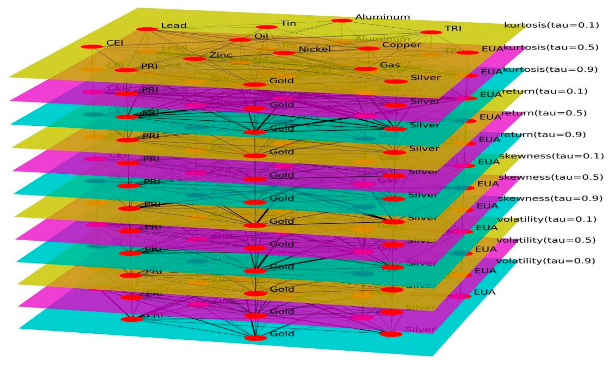
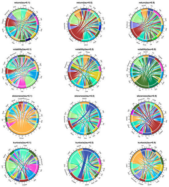
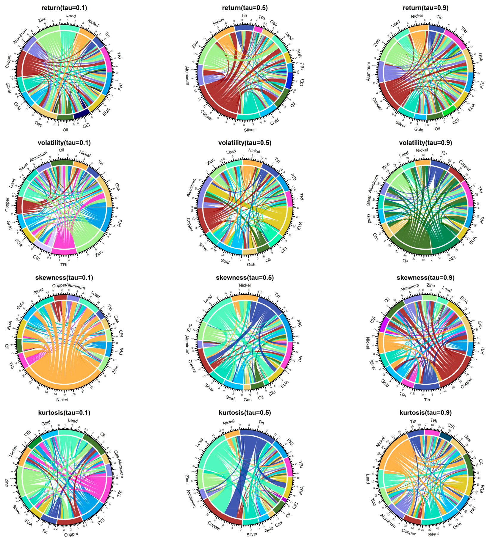
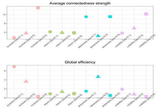
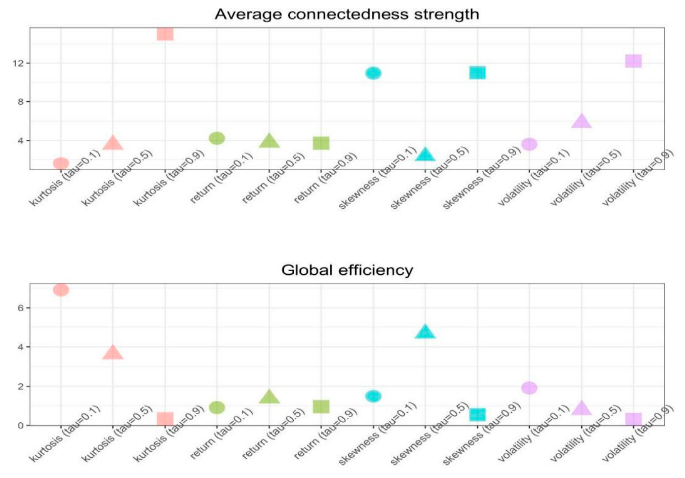
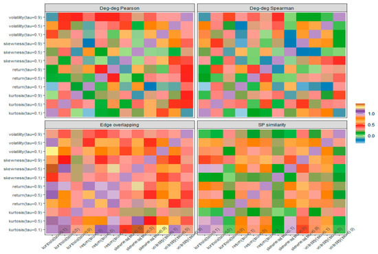
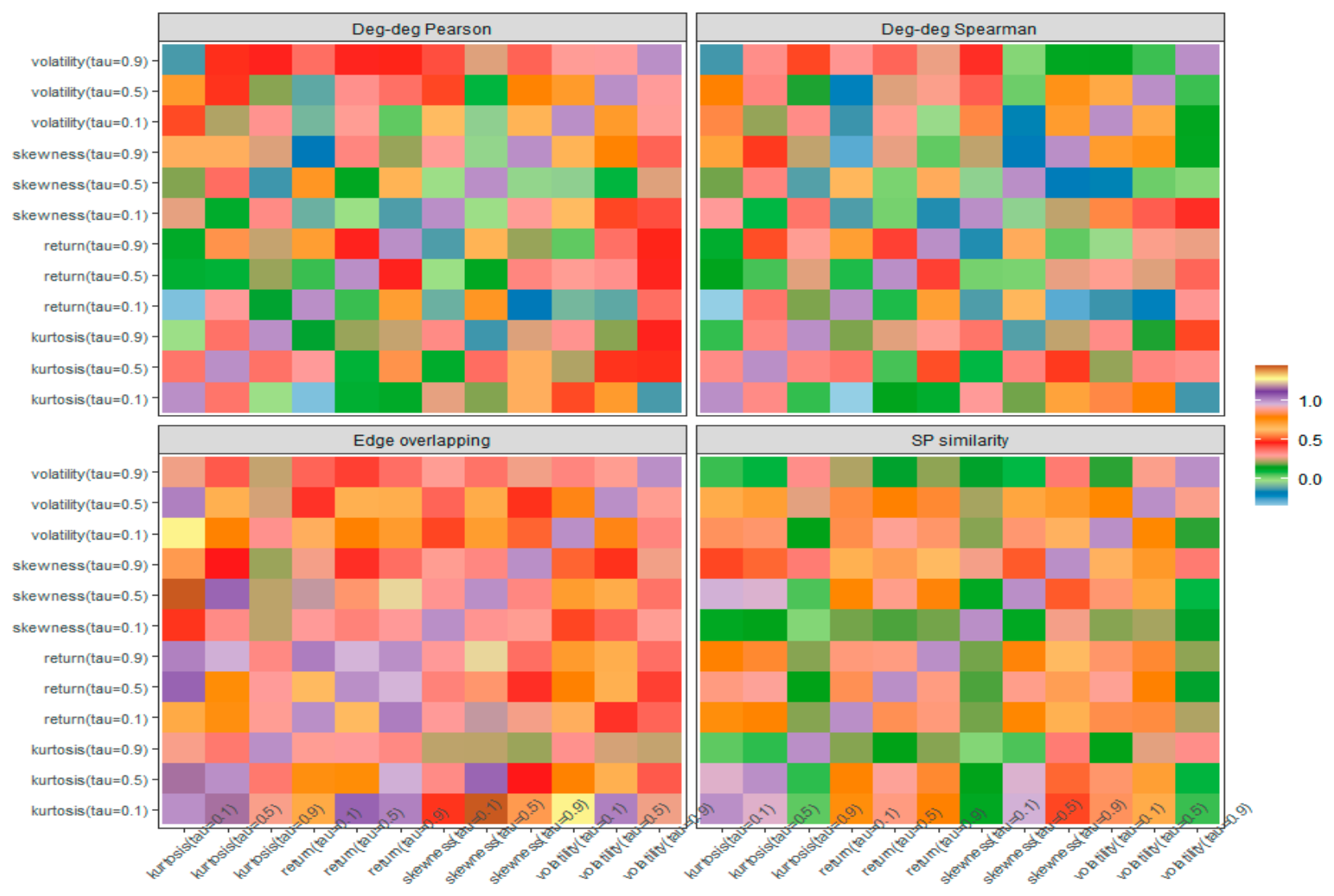
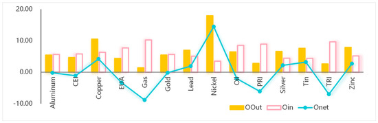
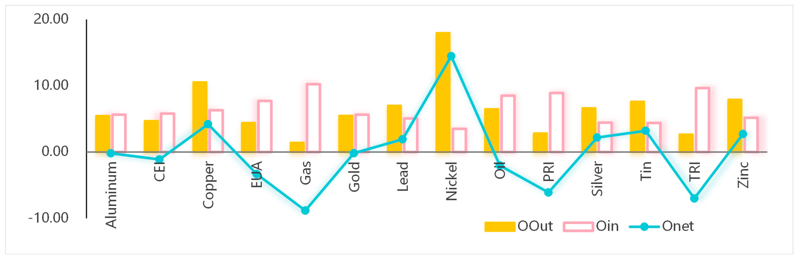
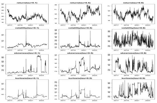
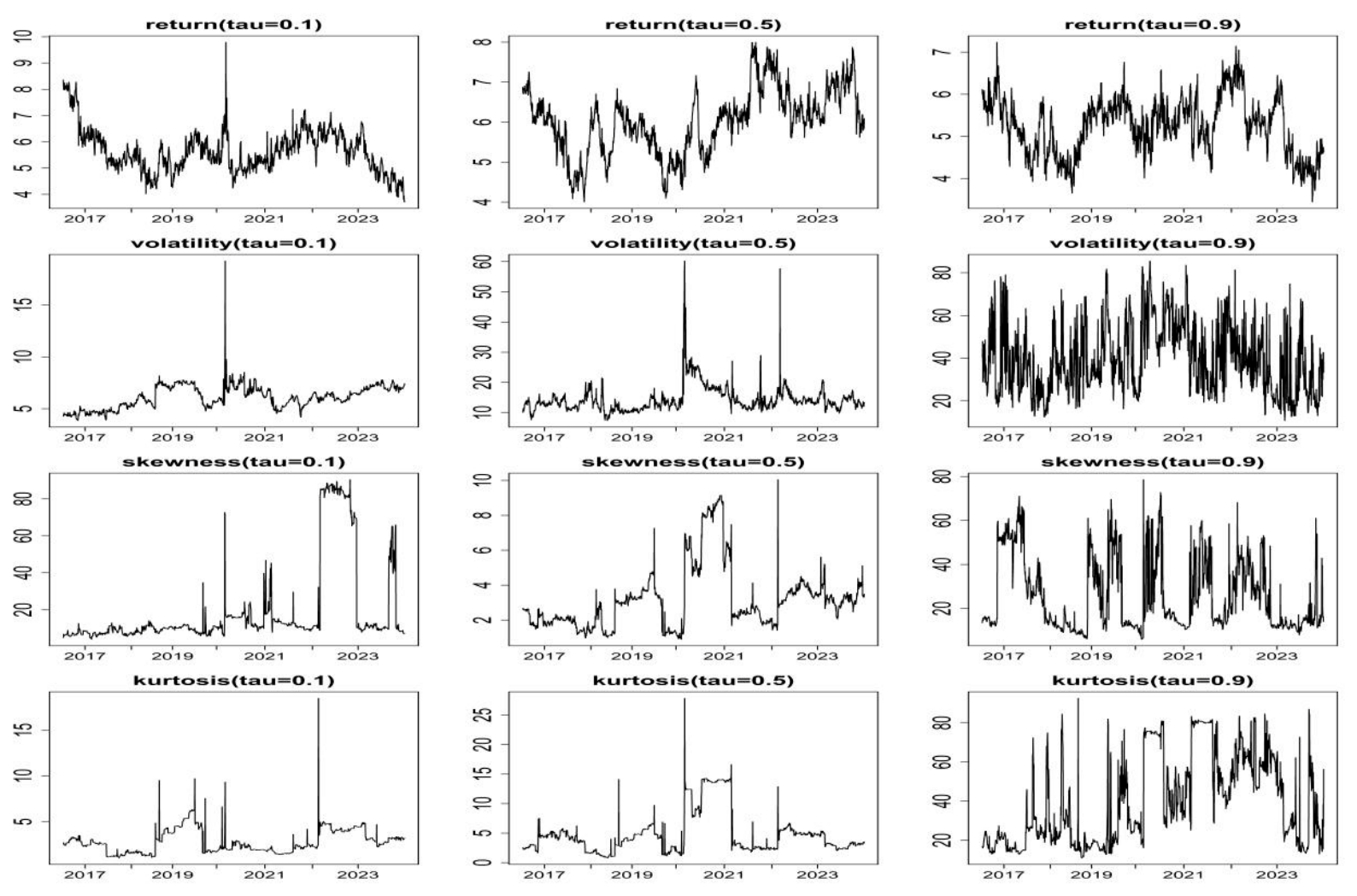
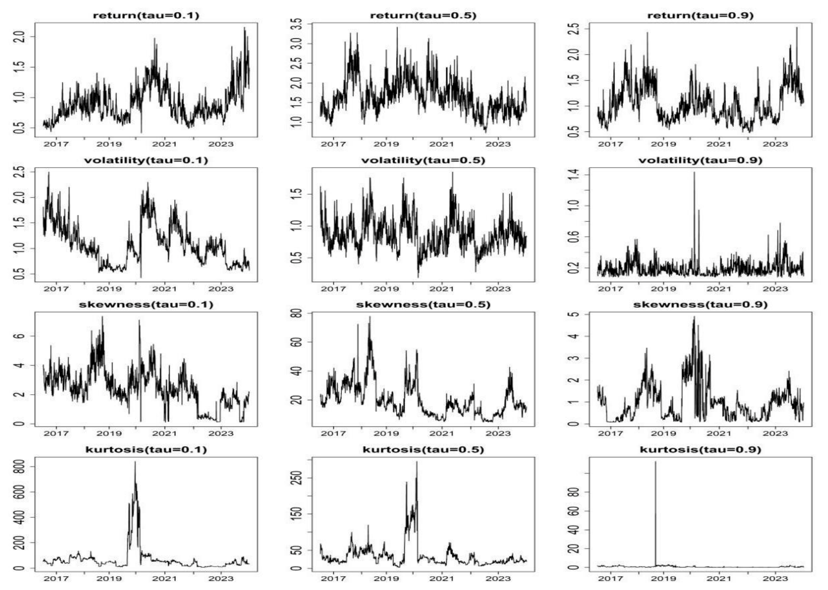
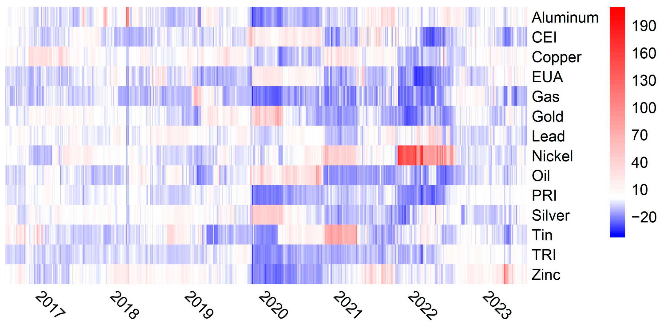

Disclaimer/Publisher’s Note: The statements, opinions and data contained in all publications are solely those of the individual author(s) and contributor(s) and not of MDPI and/or the editor(s). MDPI and/or the editor(s) disclaim responsibility for any injury to people or property resulting from any ideas, methods, instructions or products referred to in the content. |
© 2026 by the authors. Licensee MDPI, Basel, Switzerland. This article is an open access article distributed under the terms and conditions of the Creative Commons Attribution (CC BY) license.