


Abstract
This study provides a multi-faceted and detailed perspective on the relationships between logistics performance, environmental degradation, and economic growth in 38 OECD countries, using each as an individual target variable. In the Analysis section, the relationship between logistics and environment is examined within a broader context, taking economic indicators into account. This examination utilizes the machine learning algorithms Random Forest (RF), Extreme Gradient Boosting (XGBoost), and Light Gradient Boosting Machine (LightGBM). For each algorithm, the dataset is split into training and testing sets using three different ratios: 90:10, 80:20, and 70:30. A comprehensive performance evaluation is conducted on each of these splits by applying 5-fold and 10-fold cross-validation (CV). Considering economic indicators, the analysis section examines how the logistics-environment relationship is shaped in a broader context using the machine learning algorithms RF, XGBoost, and LightGBM. MSE, MAE, RMSE, MAPE, and R2 metrics are utilized to evaluate model performance, while MDA and SHAP are employed to assess feature importance. Furthermore, a bee swarm plot is leveraged for visualizing the results. The XGBoost algorithm can successfully predict carbon dioxide (CO2) emissions from transport and economic growth with high accuracy. However, the logistics performance model achieves high performance only with the LightGBM algorithm using a 90% train, 10% test split, and 5-fold CV setup. Based on the variable importance levels of the best-performing algorithm for each of the three target variables separately, the prediction of logistics performance is largely dependent on the economic growth predictor, and secondly, on the trade openness predictor. In predicting CO2 emissions from transport, economic growth is identified as the most effective predictor, while logistics performance and trade openness contribute the least to the prediction. The findings also reveal that transport-related emissions and environmental indicators are prominent in the prediction of economic growth, whereas logistics performance and trade openness play a supportive, yet secondary role.
1. Introduction
The logistics sector plays a crucial role in enhancing economic efficiency, supporting national and international trade, and strengthening global integration. As the backbone of trade, logistics constitutes a fundamental component in sustaining economic activities worldwide [1]. Furthermore, by improving accessibility, this sector significantly influences individuals’ socio-economic conditions and occupies a central position in the 2030 Sustainable Development Goals (SDGs) as a critical component of global sustainable growth [2]. Transportation is integrated into several SDGs, including sustainable transport, sustainable cities, health, energy, economic growth, infrastructure, and human settlements. In the face of increasing demand for transportation, it remains challenging—yet essential to combat issues such as rising CO2 emissions, declining air quality, and increasing traffic congestion while simultaneously addressing travel needs and improving access to opportunities, goods, and services for all individuals. As the logistics sector seeks to meet growing demand, it confronts the substantial challenge of reducing CO2 emissions. The escalating severity of environmental concerns underscores the necessity of evaluating the sustainability of this sector.
The transportation sector constitutes one of the world’s leading service industries. The establishment and utilization of transportation services greatly facilitate economic activities and contribute to the achievement of national and socio-economic development goals [3]. Therefore, a priority is to reduce CO2 emissions and establish a low-carbon, environmentally non-polluting economy.
Investments in logistics infrastructure have been shown to support economic growth through a range of positive effects. Capital investments in the logistics sector optimize economic efficiency by minimizing transaction costs and enhancing resource allocation and productivity levels [4]. Affordable and high-quality transportation services play an encouraging role by prompting firms to revise their organizational structures and reduce inventories. In doing so, firms may benefit from economies of scale by consolidating production and distribution points and increasing production quantities [5]. Economies with advanced logistics networks attain increasing economic gains. Logistics is frequently regarded as a “third source of profit,” aside from raw materials and labor, and the logistics sector is characterized as the “main artery” of the national economy [1]. In this context, the logistics sector has become an integral component of economic development strategies in the modern era. Although improved logistics performance is the key to economic growth and competitiveness, it simultaneously constitutes a source of concern regarding environmental pollution and CO2 emissions. Logistics firms are confronted with mounting pressure to reduce greenhouse gas emissions as part of the global effort to achieve CO2 mitigation targets [6].
The growing environmental concerns have drawn the attention of both scholars and policymakers toward identifying the determinants of environmental pollution and its contributing aspects to environmental degradation. The components associated with environmental degradation are linked to a country’s energy consumption profile and economic development objectives. Although this has played a role in identifying the determinants of environmental pollution, most studies restrict their analyses by associating only total energy consumption and economic growth with environmental pollution—particularly CO2 emissions [7]. However, CO2 emissions emerge not only as a function of income level but also as a consequence of other factors such as the transportation sector [8], energy consumption, foreign trade (trade openness), and financial development [9].
The conceptual foundation of these factors is associated with various theoretical approaches. In this regard, the variables used in this study are grounded in theoretical perspectives that explain the logistics-growth-environment nexus in the literature. First, the Environmental Kuznets Curve posits that economic growth initially increases environmental degradation, yet after reaching a certain income threshold, environmental quality may begin to improve [10]. Accordingly, while economic growth elevates CO2 emissions through logistics activities and energy consumption [11,12,13,14], in more advanced economic stages, sustainable transport infrastructure and innovative logistics practices may foster emission reductions [15,16]. Therefore, this study expects economic growth to be one of the strongest predictors of CO2 emissions, whereas the influence of logistics performance on emission prediction is anticipated to emerge as a combined outcome of these theoretical mechanisms.
Additionally, the Porter Hypothesis asserts that environmental regulations may stimulate innovation, leading to more efficient, cost-effective, and eco-friendly production systems [17]. This implies that sustainable logistics can both reduce environmental impacts [18] and support economic growth [19]. Furthermore, the framework linking logistics, the environment, the economy, and trade openness reveals that increases in foreign trade volumes boost logistics activities and thereby foster economic growth [20] yet can simultaneously raise transportation-based carbon emissions [21,22]. An efficient logistics structure reduces trade costs, facilitates participation in global value chains, and consequently attracts foreign investment to the country [1,23]. Time delays in transportation significantly reduce trade volumes [24], while Coto-Millán et al. [25] proved that logistics performance increases both growth and technical efficiency at the global level. Improvements in logistics infrastructure enhance supply chain efficiency, reduce trade costs, and shorten delivery lead times–thus increasing trade openness and supporting economic growth through economies of scale [26].
Based on this framework, logistics performance constitutes not only a component of economic activity but also a crucial driver of environmental degradation. In line with these theoretical approaches, the present study assumes that the relationships among logistics performance (LPI), economic growth (GDP), and transport-induced CO2 emissions may exhibit a multidimensional and nonlinear structure. Therefore, using each of the target variables individually as the dependent variable within the model aims to make bidirectional and indirect effects among variables visible.
This research seeks to contribute to literature in three ways. First, it offers a transportation-specific focus within 38 OECD member countries (Appendix A), providing a broader geographical and temporal outlook on logistics performance and transport-related CO2 emissions compared to previous studies. Second, while most prior studies rely on traditional econometric models, this research employs machine learning algorithms—RF, XGBoost, and LightGBM—as its methodological approach. Third, by treating the Logistics Performance Index (LPI), Gross Domestic Product (GDP), and CO2 emissions from transport separately as target variables, the study provides a multidimensional and detailed perspective on the relationships among them. In line with these objectives, the study evaluates the relationship between logistics performance, environmental degradation, and the economy using data from the selected countries, identifying the key factors affecting the prediction of the target variables. The primary aim of this study is not to construct a perfect prediction tool, but rather to reveal how the features contribute to the target variables.
The article is structured into four sections. Following Section 1, Section 2 presents materials and methods. Section 3 includes the results and discussion, and the study concludes with Section 4, conclusions. The study provides policy insights to support the transformation of the logistics sector into a more sustainable form across OECD countries.
2. Materials and Methods
The CO2 emission intensity of the transportation sector is a critical indicator for evaluating the dependence of economic development on CO2 emissions within this sector. Owing to differences in socioeconomic conditions and resource structures across regions, the CO2 emission intensity of the transportation sector may exhibit spatial variation. The level of CO2 emission intensity primarily depends on logistics performance and the structure of economic development. In this context, the features employed to estimate the aforementioned factors are as follows: LPI, GDP, trade openness, and CO2 emissions from transport. The analysis utilizes data for the years 2007, 2010, 2012, 2014, 2016, 2018, and 2022. Although the LPI report expected to be published in 2020 was released in 2023 due to disruptions caused by the pandemic and the global supply chain crisis, the LPI dataset was included in the World Bank (WB) database within 2022; therefore, the 2022 data are used in the study.
The primary reason for selecting the RF, XGBoost, and LightGBM algorithms in this study is that these three methods are considered tree-based ensemble models that provide high prediction performance, strong generalization capacity, and stable results in the literature on structured data [27,28,29]. According to Zhao et al. [30], some tree-based ensemble methods exhibit better and more accurate prediction performance compared to some other models. Furthermore, the decision tree structures of RF, XGBoost, and LightGBM are the most suitable options in terms of model explainability, as they allow for a detailed examination of variable importance using both permutation importance and SHAP values.
In this research, LPI, CO2 emissions from transport, and GDP are examined separately as target variables. All other remaining variables are treated as features. The variable type consists of continuous data, and no missing values are present in the dataset. The analyses are performed using Spyder (version 5.5.1) with Python (version 3.12.3) using tree-based algorithms, namely RF, XGBoost, and LightGBM. The dataset, consisting of 264 observations and three different target variables, was divided into training and testing sets using 90:10, 80:20, and 70:30 split ratios. The variables utilized in the study are presented in Table 1.
Table 1.
Variable description.
The process of forecasting logistics performance, CO2 emissions from transport, and macroeconomic indicators using tree-based ensemble learning algorithms consists of five main stages:
- Data loading and preprocessing: Data for 38 countries were imported into the software, and skewness analysis was conducted to understand the distributional characteristics of numerical variables and to identify skewed distributions that could negatively impact machine learning model performance. Furthermore, the data was split into training and testing sets using 90:10, 80:20, and 70:30 ratios. The issue of overfitting is also identified, which manifests as high performance on the training set but poor performance on the testing set [41].
- Hyperparameter optimization: Each algorithm possesses its own unique hyperparameter values. To determine these values, optimization was performed using 5-fold and 10-fold Grid Search CV; the model was then trained on the entire training dataset using the best hyperparameters.
- Model evaluation: The performance on the test dataset was assessed using mean square error (MSE), mean absolute error (MAE), root mean squared error (RMSE), and mean absolute percentage error (MAPE). In addition, R2 was calculated to measure the generalization capability of the model.
- Feature importance analysis: The contribution of each feature to the model predictions was computed using SHAP. Furthermore, Mean Decrease in Accuracy (MDA) was applied to measure feature importance and evaluate the effect of each feature on variance reduction.
- Reporting and visualization of the results: The performance metrics (MSE, MAE, RMSE, MAPE, R2-test and R2-train) were recorded for each target variable. SHAP and MDA importance scores were tabulated, and TreeSHAP values for each target variable were visualized using beeswarm plots.
The five steps listed above are applied separately for each algorithm, using logistics performance, GDP and CO2 emissions from the transport as the target variables.
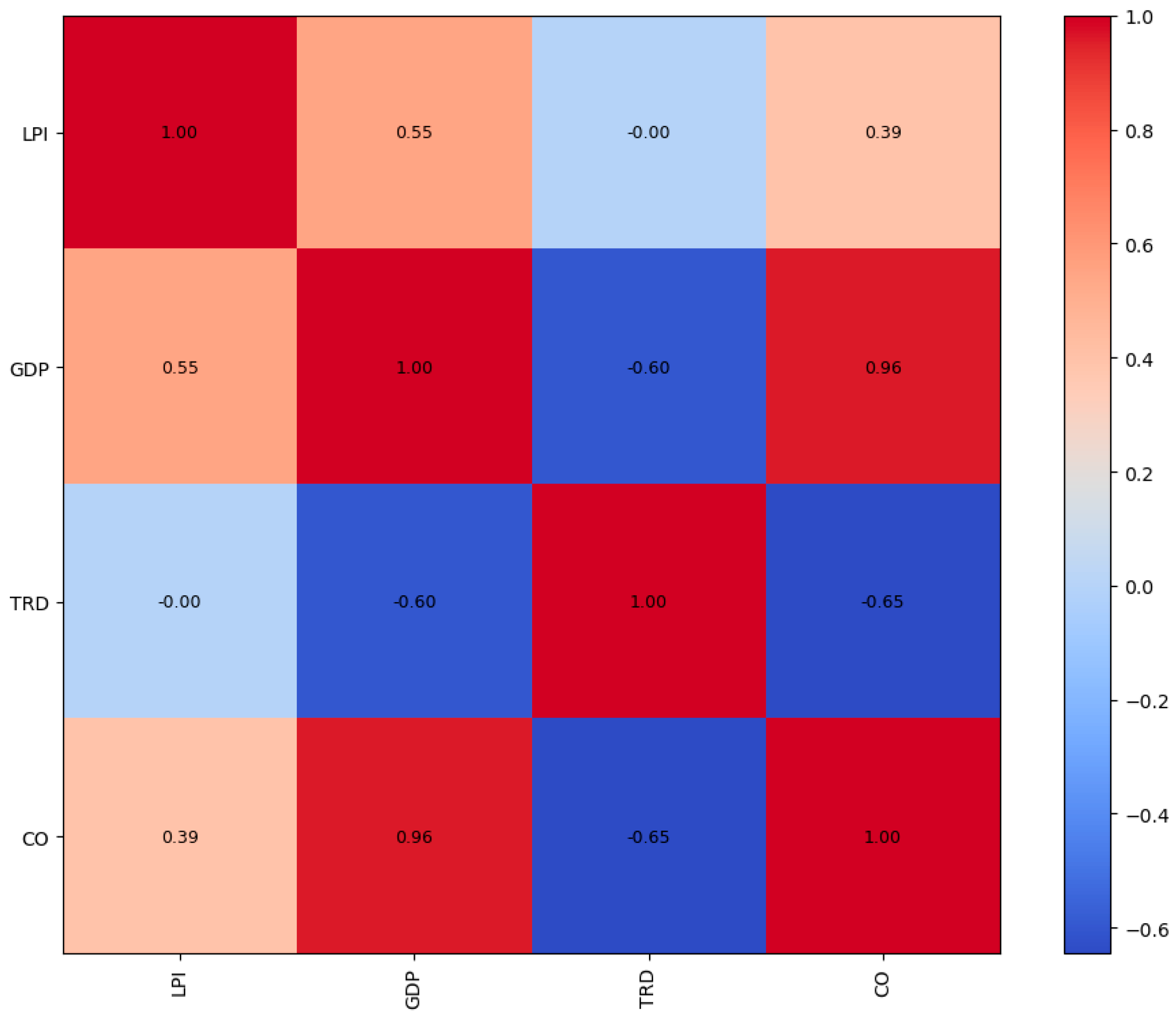
According to Figure 1, there is a very strong correlation between the GDP and CO variables in the dataset. This finding suggests that the variables represent similar economic structures and constitutes an initial indication of potential multicollinearity. However, multicollinearity does not arise solely from correlations between two variables; rather, it occurs when the variance of one independent variable is jointly explained by multiple independent variables. Therefore, the presence or source of multicollinearity cannot be conclusively determined based solely on correlation coefficients; multiple collinearity diagnostics such as the Variance Inflation Factor (VIF) are required [42].
Figure 1.
Correlation Matrix.
A high VIF value indicates that the corresponding feature exhibits strong correlation with other input variables [43]. A VIF value below 4 indicates that no multicollinearity problem exists, which is the desired situation. Conversely, exceeding a VIF value of 5 signals is a problematic level of linear dependence among variables [42]. Although RF is considered robust against multicollinearity [44], previous research has shown that when multicollinearity is present in the data, the computed feature importance scores may not yield a meaningful representation [45,46].
The results of the multicollinearity analysis for each target variable are presented in Table 2. The VIF belonging to the algorithm that yielded the best model performance for each target variable is presented in Table 2.
Table 2.
VIF Values.
During the analysis, multicollinearity was detected in only one feature. To mitigate the issue of multicollinearity, when LPI was used as the target variable, the CO feature was removed from the model, which successfully resolved the problem [27]. A wrapper-based Backward Feature Elimination approach was applied [46,47]. In the alternative model specifications, independent variables were removed one at a time, and the R2 values obtained from the training and test sets were compared. The feature set that yielded the highest generalization performance was selected.
2.1. Data Limitations
Due to the biennial publication of the LPI report by the WB, the data is limited to a seven-year period. Machine learning algorithms, particularly tree-based models, generally exhibit higher generalizability and more robust performance with larger datasets. The relatively small sample size in this study restricts the ability to fully capture the potential complexity of the model and confirm the robustness of the results. Furthermore, since the analysis was conducted using data from 38 OECD countries, a global generalization cannot be made.
The irregular and sparse time intervals within the dataset prevent us from examining the short-term or annual dynamics among the analyzed economic, commercial, and environmental indicators. This situation may limit the model’s capacity to reflect rapid changes in the transport sector, such as technological innovations or sudden policy shocks. Moreover, factors such as political fluctuations, the level of technological development, urbanization rate, and infrastructure investments, which could potentially influence the variables used in this study, were not included in the algorithm. The exclusion of such factors from the model may cause some of the estimated relationships to reflect the influence of these unobserved mediating variables.
Although the results obtained from RF, XGBoost, and LightGBM establish predictive relationships, reliably establishing and verifying causal relationships requires additional econometric analyses and more advanced causality tests. Therefore, the findings highlight priority areas and strong predictive linkages for policymakers but should not be interpreted as definitive causal relationships.
2.2. Determination of Model Hyperparameters
Hyperparameter initialization is a laborious yet essential task, as it significantly affects the performance of machine learning algorithms [48]. Tuning refers to the process of identifying the optimal hyperparameters of a learning algorithm for a given dataset. Random Forest is known to produce strong results even with default parameter settings and without the need for extensive parameter adjustment or feature scaling [49]. In fact, Probst et al. [50] measured the tunability of algorithmic hyperparameters and concluded that Random Forest is considerably less tunable than algorithms such as Support Vector Machines. The belief that default values of these parameters provide strong empirical predictive performance is widespread, and this is partially why Random Forest has become highly popular [51].
A crucial tool for evaluating the performance of an algorithm under different hyperparameter configurations is K-fold CV. This approach involves training multiple models on various subsets of the input data and is used to assess how well a model captures general patterns and similarities in data it has never encountered before [52]. In the literature, the value of k is commonly selected as five or ten to strike a balance between computational efficiency, low bias, low variance, and high predictive accuracy [53]. Repeating the entire CV procedure multiple times and averaging the resulting scores provides more reliable outcomes, as the variance of the estimate is reduced [54].
The optimal parameters for each algorithm that achieved the most successful prediction of the target variables were determined using the training parameters provided in Appendix B. Appendix B summarizes the results of the model optimization Random Forest, XGBoost, and LightGBM across different target variables. For each target variable, the hyperparameter values corresponding to the highest model performance were identified. This finding demonstrates that the model requires different configurations to most accurately predict each target variable.
2.3. Performance Evaluation Criteria
R-squared (R2) is a statistical metric that indicates the proportion of variance in the dependent variable that is explained by the features in a regression model [55]. In other words, it reflects how well the model fits the data. In model evaluation, the closer the R2 value is to 1, the higher the similarity between the predicted and observed values and, consequently, the greater the predictive accuracy of the model [56]. In this study, R2, RMSE, MSE, MAE, and MAPE are used as performance criteria. R2 training scores are also included in the tables to detect the presence of the overfitting problem.
2.3.1. LPI Model Performance
The model performance of the LPI target variable varies across three different algorithms and three distinct train–test splits. The performance evaluation results of the three applied algorithms for the LPI are presented in Table 3.
Table 3.
Performance Scores for Target Variables.
According to the results obtained from Table 3, it is observed that algorithms with relatively high predictive power—such as Random Forest with a 90:10 split and XGBoost with an 80:20 split—exhibit overfitting issues. This target variable cannot be strongly explained by the existing independent variables in most of the algorithms applied. However, since the highest R2 (test) value, the lowest RMSE, the lowest MAPE, and the lowest MAE for LPI are achieved by the LightGBM algorithm with the 90:10 split and 5-fold CV, it is evident that LightGBM provides the best performance in this study. Therefore, LightGBM should be preferred for LPI forecasting just to reduce the absolute error rate and ensure model stability.
2.3.2. GDP Model Performance
In GDP forecasting, all algorithms demonstrate remarkably high performance. All R2-test values range between 93% and 98%. Moreover, no overfitting is observed in any of the algorithms conducted for the GDP target variable.
According to Table 4, the XGBoost algorithm demonstrates the best performance under the 90:10 train-test split with both 5-fold and 10-fold CV settings. These results yield the highest test R2 values and the lowest error metrics. The fact that XGBoost’s training and test R2 values are so close to each other indicates that the model fits the data very well while simultaneously exhibiting excellent generalization capability. Owing to this optimal balance and the low error rates, XGBoost emerges as the most reliable and recommended model for GDP forecasting.
Table 4.
Performance Scores for the GDP Target Variable.
2.3.3. CO Model Performance
CO forecasting demonstrates high accuracy across all algorithms and all train–test split configurations, and once again, the XGBoost algorithm exhibits the best overall performance. The corresponding results are presented in Table 5.
Table 5.
Performance Scores for the CO Target Variable.
XGBoost, under the 80:20 train–test split and the 5-fold CV configuration, provides both strong generalization performance and the lowest mean absolute error among all algorithms. By minimizing the risk of overfitting and delivering the best overall accuracy, the XGBoost (80:20, 10-fold) configuration has been identified as the most suitable choice.
2.4. Feature Importance
Although machine learning offers high predictive accuracy, the prediction process itself is not directly observable, which places it within the black-box model domain [57]. To enhance interpretability in tree-based ensemble methods, a common feature importance measure is the count of how many times each feature is selected across all individual trees within the ensemble [58]. There are numerous feature importance metrics available in machine learning algorithms. Mean Decrease in Impurity (MDI)—also referred to as Gini Importance or Entropy—aggregates the gain associated with all splits made on a given feature and is mostly used in classification problems. MDA, also known as permutation importance, evaluates a feature’s importance by permuting its values in the test set and comparing the resulting error with the original test error. MDA measures the increase in mean squared error when a feature is randomly permuted, which quantifies how much prediction accuracy deteriorates when that feature is disrupted. The greater the increase in error, the more important the feature, since this indicates that the feature plays a critical role in model prediction performance. By definition, MDI is strongly dependent on the tree structure and can only be computed for tree-based models, whereas MDA represents a form of permutation importance that can be applied to any predictive model [59].
Lundberg and Lee [60] introduced Shapley Additive Explanations (SHAP), which integrate game theory with the interpretation of machine learning models to attribute a contribution value to each feature for a specific prediction [61]. SHAP therefore explains the importance of predictors in forecasting outcomes. A positive or negative SHAP value indicates whether a feature influences the predicted outcome positively or negatively, respectively [62]. SHAP quantifies both the direction and magnitude of feature contributions to model predictions and enables the visualization of these contributions [63]. SHAP provides valuable insights into feature importance rankings and interactions within complex datasets, contributing to the explainability of the model’s decision-making mechanisms [57]. By employing Shapley values from game theory, SHAP assigns an importance score (SHAP value) to each feature for a given prediction [64].
The bee swarm plot visualizes the features that the model considers most influential when predicting the target variable and shows how the feature values affect the prediction. In this graph, each dot represents an individual observation; the color denotes the magnitude of the feature value, while its position on the X-axis indicates the effect of that feature on the model’s prediction [65].
In the analysis, two complementary metrics are used to determine feature importance in the XGBoost algorithm, which demonstrated the highest performance for all target variables. These metrics allow ranking features based on their contribution to the model’s predictive power. The variable importance results indicate the extent to which each variable contributes to the model’s ability to predict the target variable; however, they do not imply any causal relationship. These metrics are MDA and SHAP values. For tree-based ensemble models such as decision trees and RF, TreeSHAP provides fast and exact solutions for computing SHAP values [66]. The TreeSHAP results are also visualized using bee swarm plots.
Although the three algorithms used in the analysis do not sufficiently explain the LPI target variable, MDA and SHAP allow the examination of the relative ranking of variables contributing to model predictions. Table 6 presents the variable importance rankings obtained from the LightGBM algorithm with the 90:10 train–test split and 5-fold CV, which was the only model that demonstrated satisfactory performance for LPI.
Table 6.
Feature importance scores for LPI.
When LPI is used as the target variable, the feature importance analysis reveals the contribution of each feature to the prediction of LPI. When the MDA metric is examined, GDP clearly emerges as the most influential predictor in the model’s forecasting performance. The MDA value demonstrates that the model’s performance decreases when the GDP data are permuted, indicating that the model relies heavily on GDP when predicting logistics performance. In contrast, the contribution of TRD to LPI prediction is relatively lower. The CO feature was removed from the model because it exhibited a high degree of multicollinearity with other features, which destabilized the model.
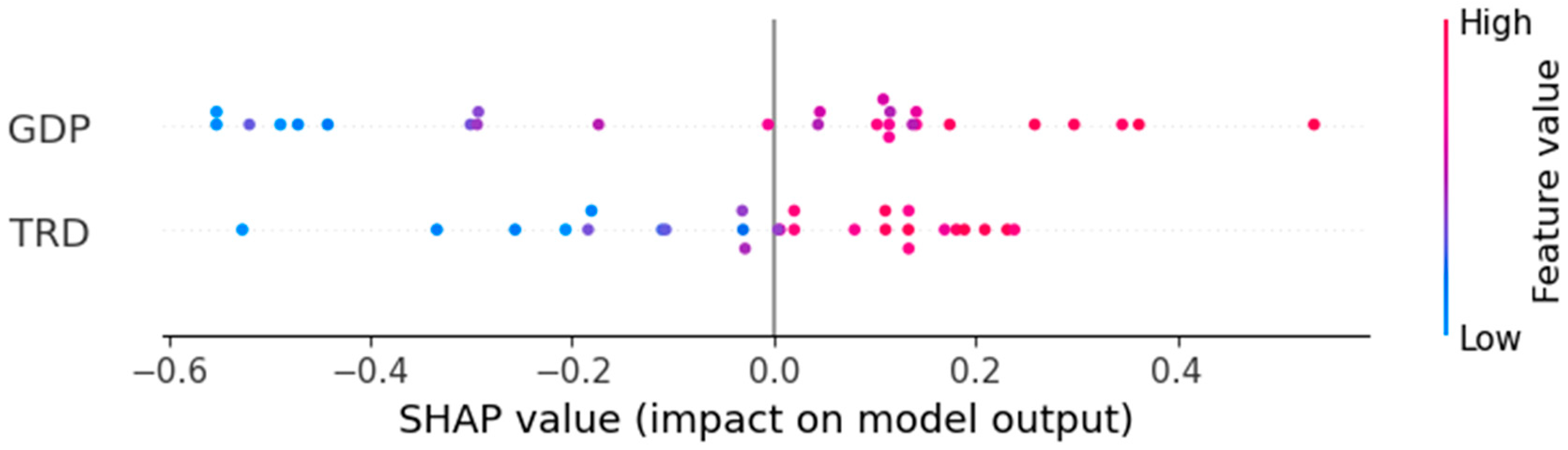
In Figure 2, the features are ranked from top to bottom according to their importance. Although the SHAP results indicate that GDP makes the strongest contribution to the prediction of LPI, the magnitude of this contribution is not sufficient to raise the overall prediction performance to a high level. High GDP values positioned on the right side of the zero line increase the predicted LPI scores. In contrast, the negative TreeSHAP values located to the left of the zero line —represented by blue points— are associated with lower and less dense GDP values, indicating that lower GDP contributes to a decrease in the predicted logistics performance. The influence of TRD on the prediction of LPI is not as strong as that of GDP. Overall, GDP emerges as a strong and directional factor in shaping the model’s predictions of LPI.
Figure 2.
SHAP Plot for the LPI Target Variable.
Table 7 presents the variable importance results from the XGBoost model with the 90:10 train–test split—using both 5-fold and 10-fold CV—where GDP is the target variable and CO, LPI, and TRD serve as predictors.
Table 7.
Feature importance scores for GDP.
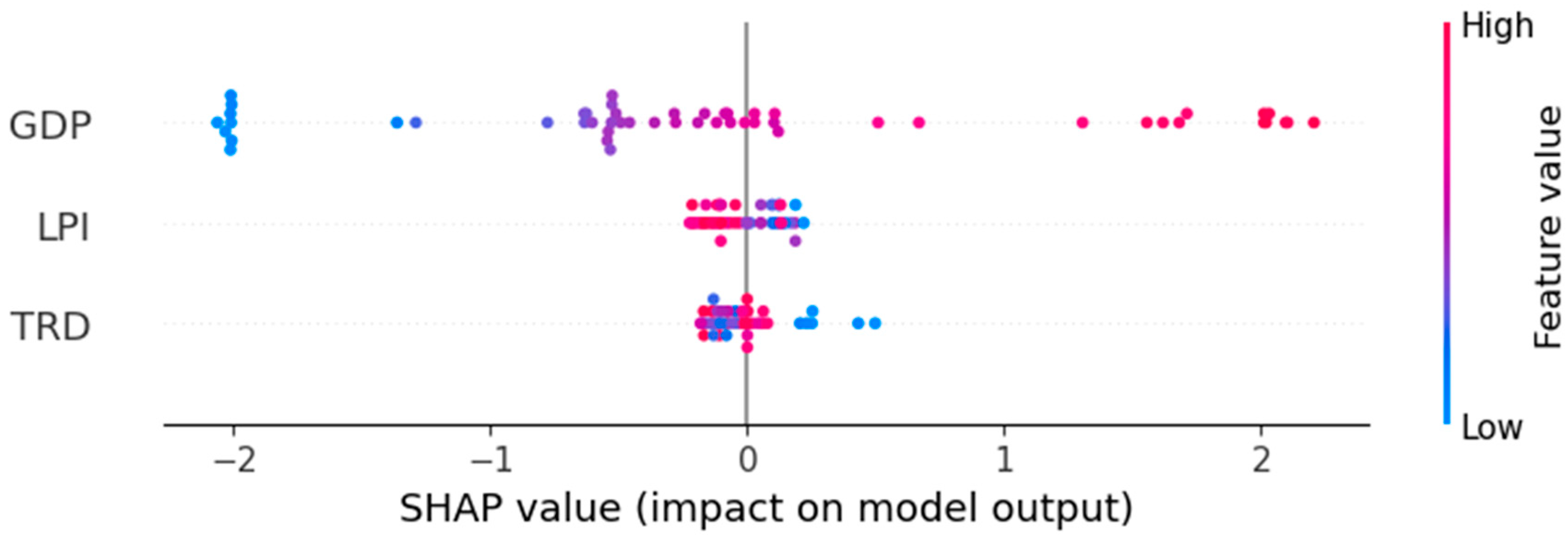
The feature importance scores calculated for the GDP target variable reveal the extent to which each feature contributes to GDP prediction. When the MDA metric is examined, the CO feature clearly emerges as the most influential predictor in GDP forecasting. This indicates that the model derives a substantial portion of the variation in GDP from the CO feature, demonstrating a strong predictive relationship between GDP and CO. Conversely, the MDA values associated with LPI and TRD show that both variables play a role in explaining GDP, although their effects are not as pronounced as that of CO. In particular, the considerably low MDA value of TRD suggests that the model has limited explanatory capability when relying on this feature.
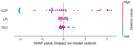
Overall, when Figure 3 is examined, the bee swarm plot visually supports the dominant role of CO in GDP predictions, the moderate contribution of LPI, and the limited effect of TRD. These results are consistent with the previous feature importance findings and indicate that environmental indicators play a decisive role in the model’s GDP estimation, while LPI and TRD have secondary levels of influence.
Figure 3.
SHAP plot for the GDP Target Variable.
Table 8 presents the variable importance results of the XGBoost model with the 80:20 train-test split and 5-fold CV, which yielded the best performance when CO was used as the target variable.
Table 8.
Feature importance scores for CO.
According to the results presented in Table 8, GDP is identified as the feature with the strongest influence on the prediction of the target variable, CO. This finding reveals that a country’s economic size and overall economic activity constitute the most important predictor of CO2 emissions from transport. The subsequent features, LPI and TRD, have comparatively more limited effects on predicting CO, suggesting that logistics performance and trade openness contribute to emission levels but to a lesser extent than GDP.
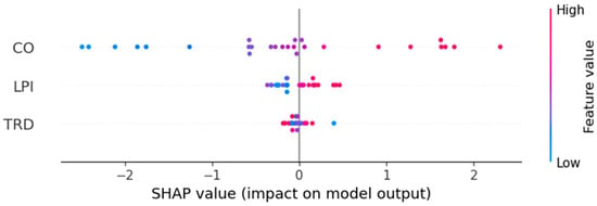
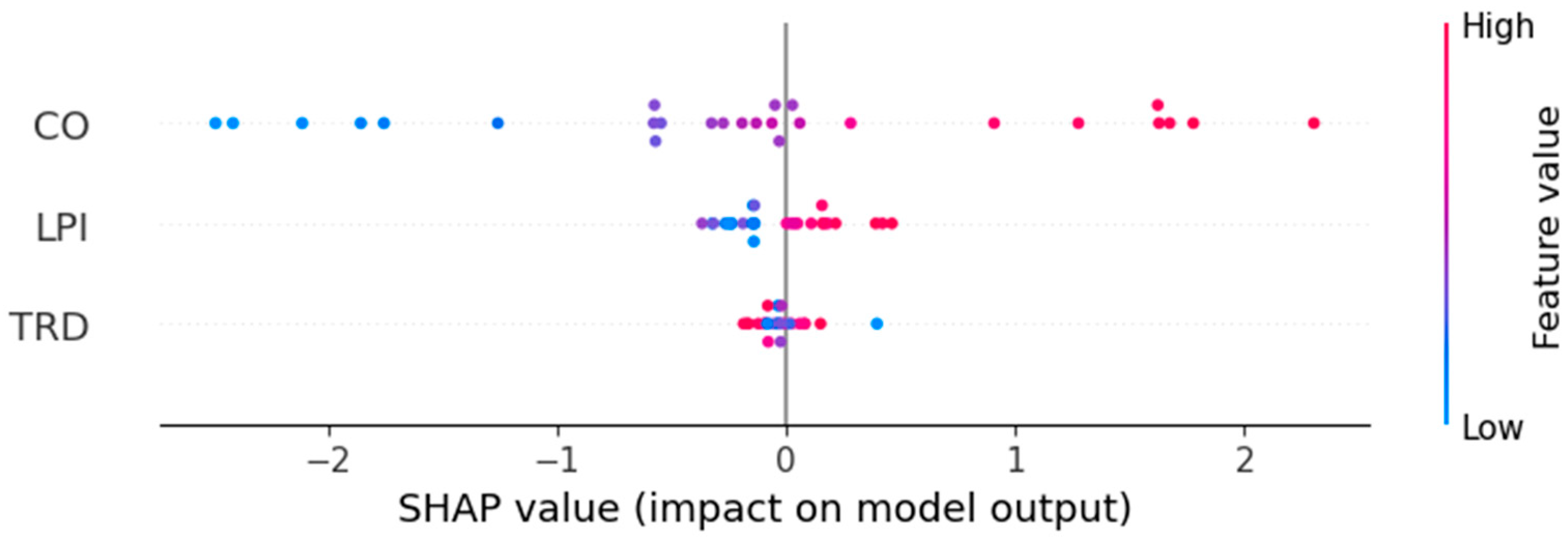
When examining the GDP feature in Figure 4, it is observed that high GDP values correspond to positive SHAP values, indicating an increasing effect on CO predictions. Conversely, low GDP values are associated with negative SHAP values, implying a decreasing influence on the predicted CO levels. This finding supports the view that economic growth increases transportation-related CO2 emissions.
Figure 4.
SHAP plot for the CO Target Variable.
LPI and TRD values appear to cluster around zero, indicating that their influence on CO prediction is comparatively lower—an outcome that aligns with the MDA results. Additionally, higher LPI and TRD values tend to reduce predicted CO levels. The dominance of blue points on the right side of the zero line reflects that lower LPI and TRD values contribute to higher CO predictions, whereas the dominance of red points on the left side of the zero line indicates that higher LPI and TRD values decrease CO predictions.
3. Results and Discussion
The study assesses the performance of the RF, XGBoost, and LightGBM algorithms in forecasting logistics performance, economic indicators, and CO2 emissions from transport, and identifies the key predictors that influence the prediction of the target variables. For the GDP and CO target variables, the overall performance evaluation of all algorithms demonstrates strong predictive capability, with performance levels varying depending on the target variable and the hyperparameter settings.
Based on the performance evaluation results obtained from the RF, XGBoost, and LightGBM analyses, the XGBoost algorithm stands out with its relatively high and robust predictive power when the target variables are economic growth and CO2 emissions from transport. The XGBoost results indicate that the algorithm is highly effective in explaining and predicting variation in economic growth and CO2 emissions from transport. XGBoost’s superiority in these variables stems from its ability to prevent overfitting more effectively than LightGBM through the use of advanced regularization mechanisms, thereby achieving better generalization performance [28]. Moreover, XGBoost’s level-wise tree growth strategy produces more stable and reliable predictions for relatively steady datasets such as GDP, compared with LightGBM’s leaf-wise strategy. RF, on the other hand, falls short of the performance achieved by these two gradient boosting algorithms, as it lacks sequential learning capabilities.
When logistics performance is used as the target variable, only one of the 18 analyses yields satisfactory results: the LightGBM model with a 90% training and 10% test split and 5-fold CV demonstrates meaningful predictive power for LPI. The fact that LightGBM achieves its best performance only under the 90:10 train-test split with 5-fold CV is a consequence of the high variance inherent in the relatively small dataset, which consists of 264 observations. The small 10% test set appears to have been, by chance, the most suitable subset for model generalization. In contrast, the weaker performance observed in the other configurations stems from the fact that the test sets in those splits capture the natural complexities and variability in the data more strongly than this specific partition.
The low performance of most algorithms in predicting LPI suggests that logistics performance is shaped not only by economic growth and emissions but also by factors not included in the model, such as foreign policy, global trade conditions, and infrastructure. LPI scores are derived from survey responses provided by logistics professionals operating in different countries [67]; therefore, they contain measurement error and perceptual biases. Moreover, LPI is determined not only by observable macro-level variables but also by factors that are difficult to measure directly, such as logistics quality, customs procedures, and infrastructure. Consequently, these omitted or imperfectly measured factors naturally limit the model’s predictive capability. In recent years, unexpected shocks to the global logistics system—such as the COVID-19 pandemic and the Suez Canal blockage—have had direct impacts on logistics performance indicators. Thus, attempting to forecast LPI scores solely on the basis of macroeconomic and environmental variables inherently excludes such sudden and often country-specific disruptions. To address this limitation, observable factors that could potentially enhance LPI forecast accuracy should include up-to-date metrics on customs and border-crossing efficiency, port/airport congestion indices, and indicators capturing last-mile delivery network density. Additionally, unobservable yet influential drivers of logistics outcomes—such as the transparency of a country’s regulatory framework, the quality of corporate governance, and the level of digitalization and intersectoral collaboration—are frequently highlighted. These factors capture the micro-operational and institutional efficiency dimensions underlying the LPI and have the potential to reduce the unexplained variance in the model.
According to the permutation importance and SHAP beeswarm plots of the best-performing algorithms for each variable, economic growth clearly emerges as the most influential predictor in the model’s forecasting performance when logistics performance is used as the target variable. This finding reveals that the prediction of logistics performance is closely linked to economic capacity, suggesting that improvements in economic output directly support logistics efficiency. In contrast, trade openness has a meaningful yet secondary influence on the prediction of logistics performance. These findings emphasize the central role of macroeconomic characteristics in determining the key drivers of logistics performance.
The variable importance findings obtained for economic growth forecasting indicate that transport-related emissions emerge as the primary predictor, while logistics performance and trade openness play supportive but secondary roles in explaining economic growth.
In forecasting CO2 emissions from transport, economic growth is identified as the most important primary predictor across the two variable-importance measures. As a country’s economy expands, production and consumption increase, which in turn amplifies the movement of goods and services, travel demand, and overall energy consumption. In other words, economic activity directly drives transportation demand, making it a key determinant of emissions. SHAP analysis shows that high trade openness and high LPI values reduce predicted CO2 emissions from transport, which may reflect more efficient logistics routes or environmentally conscious trade mechanisms. Conversely, lower levels of trade openness and LPI are associated with higher predicted emissions. This may be attributed to the fact that low trade openness forces domestic markets to rely on less efficient production and transportation systems, thereby increasing emissions. The variable importance result presented here reflects the extent to which each variable contributes to the model’s ability to predict the target variable and does not imply any causal relationship.
4. Conclusions
Logistics performance represents both a driver and an outcome of multiple dimensions of sustainability. While logistics performance stimulates economic activity and contributes to national income, it simultaneously faces increasing pressure due to the environmental degradation it triggers through CO2 emissions. Accordingly, this study extends prior research on logistics performance, economic variables, and environmental deterioration by providing an integrated interpretation of their interrelationships. Understanding the influence of CO2 emissions from transport, trade openness, economic growth, and logistics performance across OECD countries can offer policymakers more precise and operational guidance for developing appropriate transportation policies.
The overall findings indicate that economic, trade, and environmental indicators should be taken into consideration in policy design for OECD countries. The data suggest that economic growth is one of the most important predictors in explaining logistics performance, indicating that logistics performance in OECD countries is influenced by macroeconomic prosperity. Therefore, to predict the future trajectory of logistics performance and secure sustainable improvements in this domain, strategic priority should not be limited to sector-specific regulations. Investments that support aggregate economic growth and policy frameworks that ensure macroeconomic stability should also be considered. In this context, the implementation of policies such as investing in multimodal transport infrastructures, strengthening port–rail integration and coastal–inland connections, establishing high-speed links between industrial zones to facilitate the faster movement of high-value goods, expanding digital customs procedures, and modernizing logistics centers with energy-efficient and digital infrastructures is of critical importance.
In the analysis where LPI is the target variable, the exclusion of CO2 emissions from the model due to its high VIF value reflects the tension arising from the natural correlation between these two components. Policies aimed at improving logistics performance typically lead to increases in efficiency and reductions in unit costs. These cost reductions, in turn, have the potential to increase total demand for logistics services by enabling more shipments and offering lower prices. This phenomenon is known as the Rebound Effect [68]. The emission reductions achieved through efficiency gains may thus be partially or fully offset by increased demand. To counteract this outcome, strategies that balance efficiency improvements with emission-restricting measures—such as carbon taxation, the adoption of environmentally friendly fuels or vehicles, and the introduction of strict emission standards for transport modes—can be implemented, even when costs decrease.
In contrast, the fact that CO2 emissions from transport are the most important predictor of GDP forecasting indicates that a critical balance is required between economic growth and environmental sustainability. Policymakers in OECD countries should not conceptualize or pursue economic expansion independently of environmental costs; instead, they should prioritize low-carbon technologies and green production processes.
Policies addressing the control and mitigation of CO2 emissions from transport should primarily account for the economic growth dynamics that are most strongly associated with predicted emission levels. Regulations targeting the economic drivers of transport demand are likely to be more effective than approaches that focus solely on logistics performance or trade policies.
Although these findings do not imply causality, they collectively propose a three-dimensional, prediction-based policy framework for decision makers: (i) supporting economic growth while (ii) enhancing logistics efficiency, and (iii) placing environmental sustainability at the core of growth strategies, while aligning trade policies with both economic and environmental objectives. Such an approach would increase the long-term resilience of both economic development and logistics systems while minimizing environmental risks.
For future research, incorporating additional variables such as technology adoption rates, the level of technological advancement, renewable energy integration in transport, and urbanization rates may enhance the explanatory power of the models. The ways in which these relationships evolve over time could be examined, particularly in response to global trends such as decarbonization and digitalization in logistics. The application of causal analysis techniques may complement the predictive approach used in this study and provide deeper insights into the mechanisms underlying these relationships. Furthermore, studies conducted across different regions could offer more detailed evidence on how varying logistical challenges influence growth dynamics. The findings also indicate that the perceptual and survey-based components underlying the LPI cannot be fully explained by macroeconomic variables alone. Therefore, it is recommended that future research integrate qualitative and survey-based indicators into existing models to improve the forecasting of logistics performance. This would enable the capture of perceptual factors that directly reflect logistics service quality, predictability in customs processes, and institutional efficiency.
Author Contributions
Conceptualization, M.B.B. and M.M.; methodology, M.B.B.; validation, M.B.B.; formal analysis, M.B.B.; investigation, M.B.B.; data curation, M.B.B.; writing—original draft preparation, M.B.B.; visualization, M.B.B.; writing—review and editing, M.B.B. and M.M.; supervision, M.B.B. and M.M. All authors have read and agreed to the published version of the manuscript.
Funding
This research received no external funding.
Institutional Review Board Statement
Not applicable.
Informed Consent Statement
Not applicable.
Data Availability Statement
The original data presented in the study are openly available in Harvard Dataverse at https://doi.org/10.7910/DVN/UPWZCT.
Conflicts of Interest
The authors declare no conflicts of interest.
Abbreviations
The following abbreviations are used in this manuscript:
| CO2 | Carbon dioxide |
| IEA | International Energy Agency |
| MAE | Mean Absolute Error |
| MAPE | Mean Absolute Percentage Error |
| MDA | Mean Decrease in Accuracy |
| MDI | Mean Decrease in Impurity |
| MSE | Mean Squared Error |
| OECD | Organisation for Economic Co-operation and Development |
| RF | Random Forest |
| RMSE | Root Mean Squared Error |
| SDGs | Sustainable Development Goals |
| SHAP | Shapley Additive Explanations |
| VIF | Variance Inflation Factor |
| WB | World Bank |
Appendix A
Table A1.
OECD Countries.
Appendix B
Table A2.
Optimal Hyperparameters for XGBoost.
Table A3.
Optimal Hyperparameters for LightGBM.
References
- Chu, Z. Logistics and economic growth: A panel data approach. Ann. Reg. Sci. 2012, 49, 87–102. [Google Scholar] [CrossRef] [Scilit]
- United Nations—Department of Economic and Social Affairs. Sustainable Development. Sustainable Transport. Available online: https://sdgs.un.org/topics/sustainable-transport (accessed on 10 August 2025).
- Abubakar, M.A.; Abdullahi, M.; Bala, K. Analysis of the causality links between the growth of the construction industry and the growth of the Nigerian economy. J. Constr. Dev. Ctries. 2018, 23, 103–113. [Google Scholar] [CrossRef] [Scilit]
- Navickas, V.; Sujeta, L.; Vojtovich, S. Logistics systems as a factor of country’s competitiveness. Econ. Manag. 2011, 16, 231–237. [Google Scholar]
- Gunasekera, K.; Anderson, W.; Lakshmanan, T.R. Highway-induced development: Evidence from Sri Lanka. World Dev. 2008, 36, 2371–2389. [Google Scholar] [CrossRef] [Scilit]
- McKinnon, A. Green logistics: The carbon agenda. Electron. Sci. J. Logist. 2010, 6, 2–9. [Google Scholar]
- Chandran, V.G.R.; Tang, C.F. The impacts of transport energy consumption, foreign direct investment and income on CO2 emissions in ASEAN-5 economies. Renew. Sustain. Energy Rev. 2013, 24, 445–453. [Google Scholar] [CrossRef] [Scilit]
- Ong, H.C.; Mahlia, T.M.I.; Masjuki, H.H. A review on energy pattern and policy for transportation sector in Malaysia. Renew. Sustain. Energy Rev. 2012, 16, 532–542. [Google Scholar] [CrossRef] [Scilit]
- Öztürk, I.; Acaravcı, A. The long-run and causal analysis of energy, growth, openness and financial development on carbon emissions in Turkey. Energy Econ. 2013, 36, 262–267. [Google Scholar] [CrossRef] [Scilit]
- Grossman, G.M.; Krueger, A.B. Economic growth and the environment. Q. J. Econ. 1995, 110, 353–377. [Google Scholar] [CrossRef] [Scilit]
- Mariano, E.B.; Gobbo, J.A., Jr.; de Castro Camioto, F.; do Nascimento Rebelatto, D.A. CO2 emissions and logistics performance: A composite index proposal. J. Clean. Prod. 2017, 163, 166–178. [Google Scholar] [CrossRef] [Scilit]
- Khan, S.A.R.; Qianli, D.; SongBo, W.; Zaman, K.; Zhang, Y. Environmental logistics performance indicators affecting per capita income and sectoral growth: Evidence from a panel of selected global ranked logistics countries. Environ. Sci. Pollut. Res. 2017, 24, 1518–1531. [Google Scholar] [CrossRef] [Scilit] [PubMed]
- Ye, C.; Zheng, Y.H.; Han, X.L.; Chen, S.J. Can increased economic complexity and reduced carbon emissions of the logistics industry go hand in hand? Evidence from countries along the Belt and Road. Adv. Clim. Change Res. 2023, 14, 789–797. [Google Scholar] [CrossRef] [Scilit]
- Rashidi, K.; Cullinane, K. Evaluating the sustainability of national logistics performance using Data Envelopment Analysis. Transp. Policy 2019, 74, 35–46. [Google Scholar] [CrossRef] [Scilit]
- Zhang, Y.; Chen, X.; Wu, Y.; Shuai, C.; Shen, L. The environmental Kuznets curve of CO2 emissions in the manufacturing and construction industries: A global empirical analysis. Environ. Impact Assess. Rev. 2019, 79, 106303. [Google Scholar] [CrossRef] [Scilit]
- Khan, S.A.R.; Sharif, A.; Golpîra, H.; Kumar, A. A green ideology in Asian emerging economies: From environmental policy and sustainable development. Sustain. Dev. 2019, 27, 1063–1075. [Google Scholar] [CrossRef] [Scilit]
- Porter, M.E.; van der Linde, C. Toward a new conception of the environment–competitiveness relationship. J. Econ. Perspect. 1995, 9, 97–118. [Google Scholar] [CrossRef] [Scilit]
- Khan, S.A.R.; Zhang, Y.; Kumar, A.; Zavadskas, E.; Streimikiene, D. Measuring the impact of renewable energy, public health expenditure, logistics, and environmental performance on sustainable economic growth. Sustain. Dev. 2020, 28, 833–843. [Google Scholar] [CrossRef] [Scilit]
- Lean, H.H.; Huang, W.; Hong, J. Logistics and Economic Development: Experience from China. Transp. Policy 2014, 32, 96–104. [Google Scholar] [CrossRef] [Scilit]
- Pan, Y.; Gu, J.; Goodof, D. The importance of trade openness and logistics performance in economic growth: A Lasso-based approach. Int. J. Data Sci. 2023, 8, 275–294. [Google Scholar] [CrossRef] [Scilit]
- Chen, F.; Jiang, G.; Kitila, G.M. Trade openness and CO2 emissions: The heterogeneous and mediating effects for the belt and road countries. Sustainability 2021, 13, 1958. [Google Scholar] [CrossRef] [Scilit]
- Kalayci, S.; Artekin, A.Ö. The Linkage between Truck Transport, Trade Openness, Economic Growth, and CO2 Emissions within the Scope of Green Deal Action Plan: An Empirical Investigation from Türkiye. Pol. J. Environ. Stud. 2024, 33, 3231–3245. [Google Scholar] [CrossRef] [Scilit]
- Irshad, R.; Ghafoor, N. Infrastructure and Economic Growth: Evidence from Lower-Middle-Income Countries. J. Knowl. Econ. 2023, 14, 161–179. [Google Scholar] [CrossRef] [Scilit]
- Hummels, D.; Schaur, G. Time as a Trade Barrier. Am. Econ. Rev. 2013, 103, 2935–2959. [Google Scholar] [CrossRef] [Scilit]
- Coto-Millán, P.; Fernández, X.L.; Pesquera, M. Impact of Logistics on Technical Efficiency of World Production (2007–2012). Netw. Spat. Econ. 2016, 16, 981–995. [Google Scholar] [CrossRef] [Scilit]
- Bayraktar, N.; Şeker, A. OECD ülkelerinde lojistik performansın uluslararası ticaret ve ekonomik büyüme üzerindeki etkileri: Panel zaman serileri analizi. Manisa Celal Bayar Üniversitesi Sos. Bilim. Derg. 2024, 22, 363–386. [Google Scholar] [CrossRef] [Scilit]
- Yu, Z.; Kanwal, Q.; Wang, M.; Nurdiawati, A.; Al-Ghamdi, S.G. Spatiotemporal dynamics and key drivers of carbon emissions in regional construction sectors: Insights from a Random Forest Model. Clean. Environ. Syst. 2025, 16, 100257. [Google Scholar] [CrossRef] [Scilit]
- Chen, T.; Guestrin, C. XGBoost: A scalable tree boosting system. In Proceedings of the KDD’16: Proceedings of the 22nd ACM SIGKDD International Conference on Knowledge Discovery and Data Mining, San Francisco, CA, USA, 13–17 August 2016; pp. 785–794. [Google Scholar] [CrossRef] [Scilit]
- Ke, G.; Meng, Q.; Finley, T.; Wang, T.; Chen, W.; Ma, W.; Ye, Q.; Liu, T.Y. LightGBM: A Highly Efficient Gradient Boosting Decision Tree. In Proceedings of the 31st Conference on Neural Information Processing Systems (NIPS 2017), Long Beach, CA, USA, 4–9 December 2017; pp. 3149–3157. Available online: https://dl.acm.org/doi/10.5555/3294996.3295074 (accessed on 10 August 2025).
- Zhao, Y.; Wang, T.; Bove, R.; Cree, B.; Henry, R.; Lokhande, H.; Turcsanyi, M.P.; Anderson, M.; Bakshi, R.; Weiner, H.L.; et al. Ensemble learning predicts multiple sclerosis disease course in the SUMMIT study. npj Digit. Med. 2020, 3, 135. [Google Scholar] [CrossRef] [Scilit] [PubMed]
- Zaman, K.; Shamsuddin, S. Green logistics and national scale economic indicators: Evidence from a panel of selected European countries. J. Clean. Prod. 2017, 143, 51–63. [Google Scholar] [CrossRef] [Scilit]
- Magazzino, C.; Mele, M.; Schneider, N. A new artificial neural networks algorithm to analyze the nexus among logistics performance, energy demand, and environmental degradation. Struct. Change Econ. Dyn. 2022, 60, 315–328. [Google Scholar] [CrossRef] [Scilit]
- Özçelik, S.E.; Töngür, Ü. Logistics performance and environmental degradation: The case of MENA countries. Ekonomi-tek 2023, 13, 198–229. [Google Scholar]
- Ahmad, A.U.; Jeevan, J.; Ruslan, S.M.M. Evaluating key drivers of green logistics performance during economic growth in African Countries. Econ. Strategy Pract. 2024, 19, 6–19. [Google Scholar] [CrossRef] [Scilit]
- Guo, M.; Meng, J. Exploring the driving factors of carbon dioxide emission from transport sector in Beijing-Tianjin-Hebei region. J. Clean. Prod. 2019, 226, 692–705. [Google Scholar] [CrossRef] [Scilit]
- Rehman, A.; Ma, H.; Ahmad, M.; Işık, C.; Ozturk, I. Estimating interlinks of carbon emissions from transportation, industrialization, and solid/liquid fuels with economic progress: Evidence from Pakistan. Int. J. Environ. Sci. Technol. 2023, 20, 1981–1996. [Google Scholar] [CrossRef] [Scilit]
- Hayaloğlu, P. The impact of developments in the logistics sector on economic growth: The case of OECD countries. Int. J. Econ. Financ. Issues 2015, 5, 523–530. [Google Scholar]
- Al-Mulali, U.; Ozturk, I. The effect of energy consumption, urbanization, trade openness, industrial output, and the political stability on the environmental degradation in the MENA (Middle East and North African) region. Energy 2015, 84, 382–389. [Google Scholar] [CrossRef] [Scilit]
- Liu, J.; Yuan, C.; Hafeez, M.; Yuan, Q. The relationship between environment and logistics performance: Evidence from Asian countries. J. Clean. Prod. 2018, 204, 282–291. [Google Scholar] [CrossRef] [Scilit]
- Wang, H.; Sua, L. Exploring Trade Openness and Logistics Efficiency in the G20 Economies: A Bootstrap ARDL Analysis of Growth Dynamics. arXiv 2025, arXiv:2509.00368. [Google Scholar] [CrossRef] [Scilit]
- Ratner, B. Statistical and Machine-Learning Data Mining: Techniques for Better Predictive Modeling and Analysis of Big Data, 3rd ed.; Chapman and Hall/CRC: Boca Raton, FL, USA, 2017; pp. 1–655. [Google Scholar]
- James, G.; Witten, D.; Hastie, T.; Tipshirani, R. An Introduction to Statistical Learning with Applications in R; Springer: New York, NY, USA, 2013; pp. 1–426. [Google Scholar] [CrossRef] [Scilit]
- Park, J.; Lee, W.H.; Kim, K.T.; Park, C.Y.; Lee, S.; Heo, T.Y. Interpretation of ensemble learning to predict water quality using explainable artificial intelligence. Sci. Total Environ. 2022, 832, 155070. [Google Scholar] [CrossRef] [Scilit]
- Lingjun, H.; Levine, R.A.; Fan, J.; Beemer, J.; Stronach, J. Random forest as a predictive analytics alternative to regression in institutional research. Pract. Assess. Res. Eval. 2018, 23, 1. [Google Scholar] [CrossRef]
- Strobl, C.; Boulesteix, A.L.; Kneib, T.; Augustin, T.; Zeileis, A. Conditional variable importance for Random Forests. BMC Bioinform. 2008, 9, 307. [Google Scholar] [CrossRef] [Scilit] [PubMed]
- Drobnič, F.; Kos, A.; Pustišek, M. On the interpretability of machine learning models and experimental feature selection in case of multicollinear data. Electronics 2020, 9, 761. [Google Scholar] [CrossRef] [Scilit]
- Diaz-Uriarte, R.; Alvarez de Andrés, S. Gene selection and classification of microarray data using random forest. BMC Bioinform. 2006, 7, 3. [Google Scholar] [CrossRef] [Scilit]
- Zhang, W.; Wu, C.; Zhong, H.; Li, Y.; Wang, L. Prediction of undrained shear strength using extreme gradient boosting and Random Forest based on Bayesian optimization. Geosci. Front. 2021, 12, 469–477. [Google Scholar] [CrossRef] [Scilit]
- Fernández-Delgado, M.; Cernadas, E.; Barro, S.; Amorim, D. Do we need hundreds of classifiers to solve real world classification problems? J. Mach. Learn. Res. 2014, 15, 3133–3181. [Google Scholar]
- Probst, P.; Boulesteix, A.L.; Bischl, B. Tunability: Importance of hyperparameters of machine learning algorithms. J. Mach. Learn. Res. 2019, 20, 1–32. [Google Scholar] [CrossRef] [Scilit]
- Scornet, E. Tuning parameters in random forests. ESAIM Proc. Surv. 2017, 60, 144–162. [Google Scholar] [CrossRef] [Scilit]
- Tchakoucht, T.A.; Elkari, B.; Chaibi, Y.; Kousksou, T. Random forest with feature selection and K-fold cross validation for predicting the electrical and thermal efficiencies of air based photovoltaic-thermal systems. Energy Rep. 2024, 12, 988–999. [Google Scholar] [CrossRef] [Scilit]
- Shebl, A.; Abriha, D.; Dawoud, M.; Ali, M.A.H.; Csámer, Á. PRISMA vs. Landsat 9 in lithological mapping− a K-fold Cross-Validation implementation with Random Forest. Egypt. J. Remote Sens. Space Sci. 2024, 27, 577–596. [Google Scholar] [CrossRef] [Scilit]
- Seibold, H.; Bernau, C.; Boulesteix, A.L.; De Bin, R. On the choice and influence of the number of boosting steps for high-dimensional linear Cox-models. Comput. Stat. 2018, 33, 1195–1215. [Google Scholar] [CrossRef] [Scilit]
- Krzywinski, M.; Altman, N. Multiple linear regression: When multiple variables are associated with a response, the interpretation of a prediction equation is seldom simple. Nat. Methods 2015, 12, 1103–1105. [Google Scholar] [CrossRef] [Scilit]
- Guo, J.; Zan, X.; Wang, L.; Lei, L.; Ou, C.; Bai, S. A random forest regression with Bayesian optimization-based method for fatigue strength prediction of ferrous alloys. Eng. Fract. Mech. 2023, 293, 109714. [Google Scholar] [CrossRef] [Scilit]
- Zhu, C.; Liu, X.; Chen, D. Prediction of digital transformation of manufacturing industry based on interpretable machine learning. PLoS ONE 2024, 19, e0299147. [Google Scholar] [CrossRef] [Scilit]
- Strobl, C.; Boulesteix, A.L.; Zeileis, A.; Hothorn, T. Bias in random forest variable importance measures: Illustrations, sources and a solution. BMC Bioinform. 2007, 8, 25. [Google Scholar] [CrossRef] [Scilit]
- Scornet, E. Trees, forests, and impurity-based variable importance in regression. Ann. L’institut Henri Poincare B Probab. Stat. 2023, 59, 21–52. [Google Scholar] [CrossRef] [Scilit]
- Lundberg, S.M.; Lee, S.I. A unified approach to interpreting model predictions. Adv. Neural Inf. Process. Syst. 2017, 30, 1–10. [Google Scholar] [CrossRef] [Scilit]
- Cao, S.; Hu, Y. Interpretable machine learning framework to predict gout associated with dietary fiber and triglyceride-glucose index. Nutr. Metab. 2024, 21, 25. [Google Scholar] [CrossRef] [Scilit]
- Li, J.; Liu, S.; Hu, Y.; Zhu, L.; Mao, Y.; Liu, J. Predicting mortality in intensive care unit patients with heart failure using an interpretable machine learning model: Retrospective cohort study. J. Med. Internet Res. 2022, 24, 183–190. [Google Scholar] [CrossRef] [Scilit] [PubMed]
- Akbulut, S.; Yagin, F.H.; Cicek, I.B.; Koc, C.; Colak, C.; Yilmaz, S. Prediction of perforated and nonperforated acute appendicitis using machine learning-based explainable artificial intelligence. Diagnostics 2023, 13, 1173. [Google Scholar] [CrossRef] [Scilit] [PubMed]
- Antwarg, L.; Miller, R.M.; Shapira, B.; Rokach, L. Explaining anomalies detected by autoencoders using Shapley Additive Explanations. Expert Syst. Appl. 2021, 186, 115736. [Google Scholar] [CrossRef] [Scilit]
- Cui, C.; Mu, F.; Tang, M.; Lin, R.; Wang, M.; Zhao, X.; Guan, Y.; Wang, J. A prediction and interpretation machine learning framework of mortality risk among severe infection patients with pseudomonas aeruginosa. Front. Med. 2022, 9, 942356. [Google Scholar] [CrossRef] [Scilit]
- Lundberg, S.M.; Erion, G.; Chen, H.; DeGrave, A.; Prutkin, J.M.; Nair, B.; Katz, R.; Himmelfarb, J.; Bansal, N.; Lee, S.I. From local explanations to global understanding with explainable AI for trees. Nat. Mach. Intell. 2020, 2, 56–67. [Google Scholar] [CrossRef] [Scilit] [PubMed]
- Arvis, J.F.; Ojala, L.; Wiederer, C.; Shepherd, B.; Raj, A.; Dairabayeva, K.; Kiiski, T. Connecting to Compete 2018: Trade Logistics in the Global Economy, the Logistics Performance Index and Its Indicators. Available online: https://openknowledge.worldbank.org/server/api/core/bitstreams/628a4f9d-7faa-54bf-97b0-f6080c6d46cd/content (accessed on 29 November 2025).
- Zha, D.; Jiang, P.; Zhang, X. Direct energy rebound effect for road transportation in China. Front. Eng. Manag. 2023, 10, 597–611. [Google Scholar] [CrossRef] [Scilit]

Disclaimer/Publisher’s Note: The statements, opinions and data contained in all publications are solely those of the individual author(s) and contributor(s) and not of MDPI and/or the editor(s). MDPI and/or the editor(s) disclaim responsibility for any injury to people or property resulting from any ideas, methods, instructions or products referred to in the content. |
© 2026 by the authors. Licensee MDPI, Basel, Switzerland. This article is an open access article distributed under the terms and conditions of the Creative Commons Attribution (CC BY) license.