


Abstract
Central America faces a defining energy-growth challenge: sustaining economic development while curbing carbon emissions. Existing decoupling and Environmental Kuznets Curve (EKC) studies for Latin America typically pool heterogeneous economies or rely on single-country cases. This study fills that gap with a country-year panel for six Central American economies spanning 1990–2023 for GDP per capita and CO2 emissions and 2000–2021 for the clustering, EKC and Random Forest analyses that additionally require energy intensity and renewable-share data, combining GDP per capita, CO2 emissions per capita, energy intensity and renewable electricity share from World Bank and Global Carbon Project data. We apply k-means clustering, PELT structural break detection, panel fixed-effects EKC estimation with Driscoll–Kraay standard errors, Dumitrescu–Hurlin Granger non-causality tests, Random Forest importance with rolling-origin cross-validation, and the Tapio decoupling index. Clustering separates higher-income, higher-renewable-share regimes (Costa Rica, Panama) from lower-income, higher-energy-intensity regimes (the other four countries). The panel EKC yields an insignificant turning point, and Granger tests find no robust bidirectional causality. Random Forest ranks renewable share and energy intensity above GDP per capita as CO2 predictors, and rolling-origin cross-validation (R-squared = 0.856) falls below naive five-fold validation (0.938). Tapio elasticities classify four countries under weak decoupling and Guatemala and El Salvador under expansive coupling. These findings indicate that Central American decoupling is structural, associated with the electricity generation mix, rather than an automatic byproduct of growth.
1. Introduction
Climate mitigation policy increasingly requires evidence at the scale where decisions are made not based on global averages but based on individual national energy systems and their trajectories. The Intergovernmental Panel on Climate Change has emphasized that limiting warming requires steep near-term reductions in carbon dioxide (CO2) emissions across all regions, even where historical per capita contributions have been small [1]. Central America is a useful test case for this requirement. The six countries considered here, Costa Rica, Panama, Honduras, Guatemala, El Salvador and Nicaragua, are similar in geographic size, tropical climate exposure and vulnerability to hurricanes and drought, yet they differ sharply in economic structure and electricity generation mix. Whether economic growth in this region can proceed without a proportional rise in emissions, and whether that pattern is uniform across neighboring economies, remains an open empirical question that this study addresses directly.
The Environmental Kuznets Curve (EKC) hypothesis, originating with Grossman and Krueger’s analysis of pollution and income [2], proposes an inverted-U relationship in which environmental degradation rises with income at low levels of development and falls once a turning point is passed. The hypothesis has been highly influential in environmental economics, but its empirical foundations have been repeatedly questioned. Stern’s widely cited critique argued that many EKC estimates rest on a fragile statistical basis, sensitive to the time period, pollutant, and econometric specification used, and that apparent turning points often do not generalize out of sample [3]. A parallel and complementary framework, decoupling analysis, asks a narrower and arguably more policy-relevant question: whether an environmental pressure grows more slowly than the economic driver associated with it (relative or weak decoupling), stays flat or falls while the economy grows (strong decoupling), or grows faster than the economy (expansive coupling). Tapio’s elasticity-based taxonomy formalizes this comparison using the ratio of the percentage change in an environmental variable to the percentage change in its economic driver, producing a small number of discrete decoupling states that are easier to communicate to policymakers than a continuous EKC curve [4]. Decoupling analysis has since been applied across sectors and regions, including recent subnational work on Latin American cities such as Medellin, Colombia, where a longitudinal sectoral analysis found a predominance of weak decoupling between 2000 and 2023, driven mainly by efficiency gains in the tertiary sector [5].
Regional evidence for Latin America and the Caribbean illustrates why panel-level econometric diagnostics matter for this literature. Jardon, Kuik and Tol tested the EKC hypothesis on a panel of 20 Latin American and Caribbean countries over 1971–2011 and found that the answer depends critically on whether cross-sectional dependence is properly modeled: under an assumption of cross-sectional independence, a statistically plausible EKC turning point emerges, but once that assumption is relaxed and cross-sectional dependence is accounted for, the long-run equilibrium relationship between income and CO2 breaks down and the EKC is rejected [6]. This finding directly motivates the diagnostic strategy adopted in the present study, in which panel unit root tests, a cross-sectional dependence test, and Driscoll–Kraay standard errors that are robust to cross-sectional and temporal dependence are reported alongside the headline EKC coefficients, rather than being treated as an afterthought.
Within Central America, the sharpest expected contrast is between Costa Rica, whose electricity system has operated on close to 100 percent renewable generation for most of the last two decades, and Honduras, Guatemala and Nicaragua, which continue to rely on a substantial share of fossil-thermal generation. Recent engineering-oriented research on the Honduran power sector illustrates both the opportunity and the difficulty of closing this gap: a scenario-based analysis of Honduras’ power sector found that an unrestricted, low-cost expansion pathway could raise the installed renewable capacity toward 80 percent while delivering cheaper electricity than the country’s current expansion plan, and that a deep decarbonization scenario could be achieved with only a small cost premium and without carbon pricing [7]. Complementary technical work by two of the present authors and collaborators on the Honduran grid, covering battery and flywheel energy storage for frequency regulation under island-mode operation [8], the economic–environmental planning of electric distribution networks under carbon emission trading and demand response [9], and simultaneous hosting-capacity assessment for distributed generation and electric vehicles [10], demonstrates that the country’s power system is undergoing active, if incremental, transition engineering. These micro-level engineering studies describe the specific technical mechanisms, storage-based frequency regulation, carbon-aware distribution planning, and hosting-capacity expansion through which a higher-renewable electricity mix of the kind associated with Cluster 2 in this study (Section 3.2) can be operationalized at the grid level in a country that currently belongs to Cluster 1. They therefore provide a concrete, engineering-level account of what “transitioning” would practically involve for Honduras, complementing this study’s panel-level finding that electricity mix, not income growth, is what structurally separates the two clusters; but they do not by themselves answer whether that transition has yet produced a measurable decoupling of national emissions from economic growth relative to Central America’s other economies.
To systematically situate this study within the broader empirical literature, a structured bibliometric search was conducted in Scopus (Elsevier) on 21 July 2026, using the advanced query TITLE-ABS-KEY((“decoupl*” OR “environmental kuznets curve” OR “ekc”) AND (“co2 emission*” OR “carbon emission*” OR “greenhouse gas emission*”) AND (“economic growth” OR “gdp”) AND (“panel data” OR “panel analysis” OR “fixed effects” OR “panel regression”)), restricted to articles and reviews in English. The search returned 609 documents (597 articles, 12 reviews), with the earliest published in 2002 and the most recent in 2026. Output in this field has grown markedly since the mid-2010s, from single digits per year before 2013 to 32 records in 2017, a first local peak of 52 in 2020, and a further rise to 81 records in 2025 (Figure 1), indicating that panel-based EKC and decoupling research is an active and still-expanding field rather than a mature or declining one.
Figure 1.
Annual publications by top 15 contributing countries, 2002–2026 (Scopus, n = 609).
The literature is concentrated in a recognizable set of environmental and energy-economics outlets: Environmental Science and Pollution Research (79 records), Sustainability (43), Journal of Environmental Management (22), Energies and the International Journal of Energy Economics and Policy (19 each), and the Journal of Cleaner Production (18). The most-cited works in the corpus anchor the field’s foundational questions, paneling evidence linking CO2 emissions, energy consumption, trade and urbanization for EU accession countries [11] (cited over 1100 times), the role of renewable energy consumption in reshaping the EKC [12] (cited over 1000 times), and EKC tests for developing-country panels [13,14], and were all published between 2010 and 2016, confirming that the panel-EKC research design used in the present study sits within a well-established and heavily cited methodological tradition. A keyword co-occurrence network built from the Author Keywords of the same corpus (Figure 2) shows three dominant, densely interlinked clusters organized around economic growth and GDP, the environmental Kuznets curve and EKC hypothesis, and CO2 or carbon emissions, with renewable energy and panel data as large secondary nodes bridging the clusters. An overlay of the same network colored by average publication years (Figure 2) shows that the foundational EKC, CO2-emission and panel-data terms average an earlier publication year (around 2020), while renewable-energy, environmental-sustainability, and technological-innovation terms average a later one (2022–2023), indicating that the field’s center of gravity has moved from testing the basic EKC hypothesis toward panel-based, renewable-energy-augmented specifications, precisely the space this study occupies.
Figure 2.
Keyword co-occurrence map. (a) Keyword co-occurrence network of bibliometric corpus (n = 609), clustered by co-occurrence structure. (b) Keyword co-occurrence network overlay, colored by average publication year. In (a), node color denotes co-occurrence cluster membership; in (b), node color denotes average publication year on the scale shown.
Author affiliations in the corpus are heavily concentrated in a small number of large emerging economies, led by China (214 documents with at least one China-based author), Turkey (93), Pakistan (73), the United States (44), Saudi Arabia and India (36 each), the United Kingdom (32), Australia (30), Malaysia (28) and Bangladesh (23); no record in the 609-document corpus carries an institutional affiliation in Costa Rica, Panama, Honduras, Guatemala, El Salvador or Nicaragua. Latin American representation in the corpus overall is thin and concentrated in the region’s largest economies: Brazil, Colombia and Mexico contribute three documents each, Chile two, and Ecuador one (Figure 3a); no other Latin American country appears at all. Document types are 98 percent articles and 2 percent reviews (Figure 3b), so the corpus reflects primary empirical research rather than a literature already summarized in reviews. Only three records mention Central America, the SICA bloc, or an individual member country anywhere in their title, abstract or keywords, and of these, only one is a genuine regional panel study: Gazeloglu and Erkilic analyze economic growth, international tourism, renewable-energy use and carbon emissions across the members of the Central American Integration System (SICA) using a 2001–2020 panel of 140 observations and a feasible generalized least squares model with panel cointegration tests [15]. That study, published in 2025, is the closest existing work to the present one, but it covers the eight-member SICA bloc, which includes Belize and the Dominican Republic alongside the six countries studied here, spans a shorter and more recent window (2001–2020 versus 1990–2023), is organized around international tourism as the central mechanism, and does not include cluster analysis, structural break detection, machine learning-based variable importance validated by rolling-origin cross-validation, or the Tapio decoupling taxonomy. This bibliometric evidence substantiates, rather than merely asserts, the gap motivating the present study: a large and fast-growing literature tests panel EKCs and decoupling relationships worldwide, a literature to which this study’s methodology directly belongs, but almost none of it has been applied to the six mainland Central American economies considered here, and the one regional panel study that does exist uses a different methodological toolkit and a different regional and temporal scope.
Figure 3.
(a) Latin American publication distribution in bibliometric corpus; (b) document-type composition. Note: This study’s six countries (Costa Rica, Panama, Honduras, Guatemala, El Salvador, Nicaragua) record 0 of 609 documents in the bibliometric corpus.
This study builds directly on a previously validated single-country methodology. Ramirez, Munoz Tabora and Melgar-Dominguez developed and applied a longitudinal machine learning and econometric pipeline, combining k-means clustering, PELT structural break detection, an Environmental Kuznets Curve model with heteroskedasticity-and-autocorrelation-consistent standard errors, Granger causality tests, Random Forest variable importance with rolling-origin cross-validation, and the Tapio decoupling index, to Honduras’ 1990–2023 energy-growth trajectory [16]. A targeted literature search conducted in July 2026 found no dedicated study applying this specific combination of clustering, panel econometrics, machine learning and decoupling-index methods to a full six-country Central American panel; regional decoupling and EKC evidence exists at a coarser Latin American-wide resolution [6] or at a single-country or subnational resolution [5,16] but not at the resolution of a comparative six-country regional panel. The present study closes that gap by extending the validated Honduras pipeline from a single-country time series to a country-year panel covering Costa Rica, Panama, Honduras, Guatemala, El Salvador and Nicaragua, with country fixed effects and panel-robust inference replacing the single-series techniques used previously.
The central research question is whether these six countries, similar in region, economy size and climate exposure, follow distinct decoupling trajectories, and if so, what explains the differences: electricity mix, economic structure, or energy policy? The remainder of the paper is organized as follows: Section 2 describes the panel data, its sources and coverage, and each of the six analytical methods used. Section 3 reports results in the same order: descriptive statistics and coverage, cross-country clustering, structural breaks, the panel EKC, panel unit root and Granger causality diagnostics, Random Forest importance and its rolling-origin robustness check, and the Tapio decoupling index by country and by cluster. Section 4 discusses these findings against the literature and the region’s policy context, and Section 5 concludes.
2. Materials and Methods
2.1. Study Area, Data Sources and Variables
This study covers six Central American economies, Costa Rica, Panama, Honduras, Guatemala, El Salvador and Nicaragua, over the period 1990–2023 (34 calendar years). All growth and emission variables in this study are measured on a per capita basis (GDP per capita, CO2 per capita); results and conclusions therefore describe per capita decoupling and should not be read as claims about total national GDP or total national emissions, which can diverge from their per capita counterparts under population growth. This yields a maximum possible panel of 204 country-year observations. Four variables were assembled for each country-year, following the variable definitions used in the original Honduras dataset so that the two studies remain directly comparable [16]: (1) GDP per capita, in constant 2015 USD (World Bank World Development Indicators, code NY.GDP.PCAP.KD) [17]; (2) CO2 emissions per capita, in tons per capita, measured on a territorial (production) basis consistent with the Global Carbon Project’s Global Carbon Budget methodology (fossil-fuel combustion and cement process emissions only; land-use-change emissions are excluded and reported separately by the Global Carbon Project), sourced from the Global Carbon Project’s Global Carbon Budget as distributed by Our World in Data [18,19]; (3) energy intensity, measured as megajoules of primary energy supply per USD of GDP (World Bank WDI, code EG.EGY.PRIM.PP.KD) [17]; and (4) the renewable share of electricity generation, in percent (World Bank WDI, code EG.ELC.RNEW.ZS) [17]. Country-year coverage for all four variables is summarized in Table 1. A derived carbon-intensity-of-output variable was computed as CO2 emissions per capita divided by GDP per capita (scaled by 1000), expressing tons of CO2 per thousand constant-2015-USD of GDP per capita, and is reported as a descriptive statistic (Table 2 and Table 3) alongside the four core variables. It is deliberately excluded from the Random Forest model described in Section 2.7 because it is constructed by dividing CO2 per capita by GDP per capita and including it as a predictor of CO2 per capita would embed the response variable inside a predictor (target leakage), artificially inflating both the variable importance and cross-validated accuracy. All data were retrieved from the World Bank DataBank and the Our World in Data CO2 and Greenhouse Gas Emissions grapher interface (filtered server-side by country and year) on 20 June 2026, using the same retrieval methodology validated against the previously published Honduras series [16], and the exact match against that published series was confirmed before assembling the remaining five countries.
Table 1.
Data coverage by country and variable, 1990–2023 (number of non-missing country-years).
Table 2.
Pooled descriptive statistics, Panel B (2000–2021, n = 131).
Table 3.
Descriptive statistics by country, Panel B means (2000–2021).
GDP per capita and CO2 emissions per capita are available for all six countries across the full 1990–2023 window, with no missing country-years. Energy intensity and the renewable electricity share have shorter and, for most countries, similar coverage windows to the ones already documented for Honduras: both are available from 2000 onward, and the renewable share generally extends through 2021, while energy intensity generally extends through 2021 as well, with a one-year advantage for Costa Rica in both series (Table 1). Because of this structure, two overlapping analysis panels are used throughout, following the same logic as the original Honduras study. Panel A comprises all 204 GDP-CO2 country-year observations (1990–2023) and is used wherever only these two variables are required: the long-run trend figures, PELT structural break detection, panel unit root tests, Dumitrescu–Hurlin Granger test on GDP and CO2, and per-country Tapio index. Panel B restricts the sample to 2000–2021 and requires non-missing values for all four core variables (GDP per capita, CO2 per capita, energy intensity and renewable share); after listwise deletion, this yields 131 of the 132 theoretically possible country-year rows (6 countries times 22 years), with a single country-year dropped for a missing renewable-share value. Panel B is used for descriptive statistics, k-means clustering, the panel EKC estimation, and the Random Forest model.
2.2. Cluster Analysis
To identify whether the six countries group into a small number of distinct energy-growth regimes rather than form a continuum, k-means clustering [20] was applied to the standardized (z-scored) values of the GDP per capita, CO2 per capita, energy intensity and renewable share in Panel B (131 country-year rows). The number of clusters, k, was selected by maximizing the average silhouette width [21] over a candidate range of k = 2 to 7, with the maximum candidate k-bounded so that no cluster would be expected to average fewer than six observations. A robustness re-clustering was also performed using only energy intensity and renewable share, the two variables most directly tied to the electricity and energy system rather than to the scale of the economy, to check whether the country groupings were an artifact of including GDP and CO2 as clustering inputs alongside the Tapio-adjacent quantities. Agreement between the two clustering solutions was measured as the percentage of country-year rows assigned to the same relative cluster ordering in both solutions.
2.3. Structural Break Detection
Structural breaks in each country’s CO2 per capita, energy intensity, and renewable-share series were identified independently, country by country, using the Pruned Exact Linear Time (PELT) algorithm for optimal changepoint detection [22], implemented in the changepoint R package [23]. The PELT identifies the set of changepoints that minimizes a penalized sum of segment-wise costs (here, changes in the mean) with a computational cost that scales linearly in the length of the series, making it an exact rather than approximate search over the changepoint locations. The penalty was set via the Bayesian information criterion (BIC) (penalty values reported in Section 3.3), and a minimum segment length of three years was imposed between consecutive breakpoints to avoid detecting changes driven by single-year noise; a modified-BIC (MBIC) penalty sensitivity check is also applied and reported in Section 3.3. CO2 per capita breaks were computed on the full 1990–2023 series (Panel A) for all six countries; energy intensity and renewable-share breaks were computed on the shorter 2000–2021 window (Panel B) for which those series are available.
2.4. Panel Environmental Kuznets Curve Estimation
The EKC relationship was estimated as a country-fixed-effects (within) panel regression of the natural logarithm of CO2 per capita on the natural logarithm of GDP per capita and its square, using Panel B (2000–2021, 131 country-year observations). Consistent with the classical Grossman–Krueger EKC specification, the model deliberately includes only GDP per capita and its square as regressors, without energy intensity or renewable share as additional covariates, so that the estimated turning point can be compared directly to the standard single-variable EKC literature; the independent contribution of energy intensity and renewable share, which Section 3.7 shows to be the strongest predictors of CO2 per capita, is captured separately by the clustering (Section 3.2) and Random Forest (Section 3.7) analyses rather than folded into the EKC regression itself:
where αi is a country fixed effect that absorbs time-invariant differences across countries (for example, geography, or the historical starting composition of the electricity grid), and the model is estimated using the within (fixed-effects) estimator implemented in the plm package [24]. A negative and statistically significant β2 is the standard signature of an inverted-U EKC, with an implied income turning point at exp(−β1/2 × β2). Because panel data of this kind commonly exhibit both serial correlation and cross-sectional dependence, and because the Jardon, Kuik and Tol result summarized in Section 1 shows that failing to account for cross-sectional dependence can produce a spuriously confirmed EKC [6], standard errors were computed using the Driscoll–Kraay panel-robust covariance estimator [25], the direct panel generalization of the Newey–West heteroskedasticity-and-autocorrelation-consistent standard errors used in the original single-country Honduras analysis [16,26], with a maximum lag of four years. For transparency, the fixed-effects Driscoll–Kraay results are reported alongside a naive pooled OLS specification without country fixed effects or panel-robust standard errors so that the effects of both corrections on the estimated coefficients and their precision can be seen directly. A 95 percent confidence interval for the income turning point was computed via the delta method, using the Driscoll–Kraay variance–covariance matrix.
ln(CO2 per capitait) = αi + β1 ln(GDP per capitait) + β2 [ln(GDP per capitait)]2 + εit
2.5. Panel Unit Root and Cross-Sectional Dependence Diagnostics
Because EKC and Granger causality estimates are only meaningful if the underlying series have well-understood stationarity properties, three complementary panel unit root tests were applied to the logarithms of GDP per capita and CO2 per capita in Panel A (204 country-year observations, 1990–2023): the Im–Pesaran–Shin (IPS) test, which averages heterogeneous augmented Dickey–Fuller statistics across units [27]; the Maddala-Wu Fisher-type test, which combines per-unit augmented Dickey–Fuller p-values [28]; and the Hadri Lagrange-multiplier test, whose null hypothesis is stationarity rather than a unit root, giving a test in the opposite direction to the IPS and Maddala-Wu [29]. Because the three tests can disagree, particularly when cross-sectional dependence is present, their joint pattern was interpreted qualitatively rather than any single test being treated as decisive. In addition, the fixed-effects EKC model was checked for residual serial correlation using the panel Wooldridge/Durbin–Watson test [24] and for cross-sectional dependence using the Pesaran CD test [30], the panel-appropriate analogues of the single-series Durbin–Watson and Breusch–Pagan diagnostics used in the original Honduras study. A second-generation panel unit root test explicitly robust to cross-sectional dependence, the Pesaran cross-sectionally augmented IPS (CIPS) test [31], was also attempted. Its published critical-value tables, however, are tabulated only for panels with at least ten cross-sectional units [31], which is above this study’s six-country panel, so a tabulated p-value could not be obtained; this is reported as an explicit small-N limitation of the CIPS methodology itself rather than as an omitted robustness check (Section 4).
2.6. Panel Granger Non-Causality Tests
Temporal precedence between GDP per capita and CO2 per capita was tested using the Dumitrescu and Hurlin panel Granger non-causality test [32], which extends the Granger framework to heterogeneous panels by averaging individual Wald statistics across units and does not require the coefficients to be identical across countries, making it more appropriate for a six-country panel with divergent economic structures than a homogeneous-panel Granger test would be. The test was applied to first-differenced GDP per capita and CO2 per capita in Panel A (204 observations, order 1), in both directions (GDP Granger-causing CO2 and CO2 Granger-causing GDP). An analogous set of panel Granger tests was run for the renewable electricity share, restricted to a balanced window that excludes 2001 (where the renewable-share series has a coverage gap for one country), testing whether renewable share Granger-causes CO2 per capita, whether CO2 per capita Granger-causes renewable share, and whether GDP per capita Granger-causes renewable share. As a transparency check and to allow for an inspection of the country-specific heterogeneity that the pooled panel test necessarily averages over, conventional single-series Granger tests (order 1) were also run for each of the six countries individually, in both directions. Because this involved twelve simultaneous hypothesis tests (six countries times two directions), Holm [33] and false-discovery-rate [34] corrections for multiple comparisons were applied to the resulting p-values. In addition, the primary Dumitrescu–Hurlin specification used the shortest feasible lag order, 1, chosen for parsimony given the short annual series available (34 years per country) and consistent with standard practice for panels of this length; the confirmation of this choice does not drive the conclusions, and a sensitivity sweep across lag orders 1 to 5 was run for the panel test to check whether the null result of no significant bidirectional causality is robust to lag selection.
2.7. Random Forest Variable Importance and Rolling-Origin Cross-Validation
A Random Forest regression model [35], implemented via the randomForest package [36] and tuned via the caret package [37], was fit to predict CO2 per capita from GDP per capita, energy intensity, renewable share, and country identity (included as a categorical predictor to allow the model to absorb country-specific fixed effects nonparametrically), pooling all 131 country-year observations in Panel B; the derived carbon-intensity-of-output variable was excluded from the predictor set for the reason given in Section 2.1. The mtry hyperparameter (number of candidate predictors considered at each split) was tuned over the full candidate range via five-fold cross-validation on the full dataset, and the final in-sample model was fit with 500 trees. Permutation-based variable importance (percent increase in mean squared error when a predictor is randomly permuted) was used as the primary importance measure, alongside the increase in node purity.
Because standard k-fold cross-validation systematically overstates a time-series model’s true predictive accuracy by allowing future years to help predict past years within the same fold structure, model performance was additionally validated using a rolling-origin (expanding year-block) cross-validation scheme, in which the model is trained only on years prior to a given origin year and evaluated on a subsequent block of held-out years, with predictions pooled across all origins before computing out-of-fold R-squared and root-mean-squared error (RMSE), rather than averaging per-fold statistics, which would give disproportionate weight to folds with few observations. This pooled-prediction rolling-origin design was a correction identified as necessary during the peer-review process for the original single-country Honduras study and was built into the panel pipeline from the outset here [16]. The main reported rolling-origin specification used an expanding training window with an initial window of 14 years (2000–2013) and a two-year forecast horizon so that the model was always trained on at least 14 annual observations per country before any prediction was scored, and the remaining 2014–2021 period yielded four expanding two-year test blocks, the two-year horizon balances having enough held-out blocks to obtain a stable pooled out-of-fold estimate against retaining enough training years in the earliest fold for a four-predictor Random Forest to be estimated reliably. Two additional specifications, a fixed-width training window with a two-year horizon and an expanding window with a one-year horizon, were run as sensitivity checks, together with the naive five-fold in-sample cross-validation result, to characterize how much of the model’s apparent accuracy depends on the validation scheme.
Within the rolling-origin scheme, the mtry was re-tuned separately inside each expanding training window using that window’s own out-of-bag error, rather than reusing the single mtry value selected by the whole-dataset five-fold cross-validation described above, so that no information from years after a given training cutoff could influence the model configuration. Three benchmark models, a naive persistence forecast using each country’s last observed value, a linear regression on GDP per capita, energy intensity and renewable share, and a country-specific historical mean, were evaluated on the identical rolling-origin folds as the Random Forest to establish whether the Random Forest’s accuracy exceeds what simpler models achieve under the same temporally honest validation design. Finally, because a six-country panel could overstate generalizability if country identity alone is driving predictive accuracy, a leave-one-country-out (LOCO) cross-validation was run, in which the model was trained on five countries and evaluated on the sixth, with the country-identity predictor omitted entirely (a held-out country has no fitted level for that predictor), to test whether the fitted relationships transfer to a country outside the estimation sample.
2.8. Tapio Decoupling Elasticity Index
Following Tapio’s original formulation [4], the decoupling elasticity for country i in year t is defined as the ratio of the percentage change in CO2 per capita to the percentage change in GDP per capita over the same interval: e_it = (%change in CO2 per capita)/(%change in GDP per capita). Year-over-year elasticities were computed for every country across the full 1990–2023 window (Panel A) and classified into the eight categories of the standard Tapio (2005) taxonomy [4]: strong decoupling (GDP growth non-negative, e < 0); weak decoupling (GDP growth non-negative, 0 ≤ e < 0.8); coupled growth (GDP growth non-negative, 0.8 ≤ e ≤ 1.2); expansive coupling (GDP growth non-negative, e > 1.2); recessive decoupling (GDP contracting, CO2 also contracting, e > 1.2); recessive coupling (GDP contracting, CO2 also contracting, 0.8 ≤ e ≤ 1.2); weak negative decoupling (GDP contracting, CO2 also contracting, e < 0.8); and strong negative decoupling (GDP contracting, CO2 rising). An earlier specification collapsed the four GDP contraction states into two; the full eight-state taxonomy is used throughout the results reported below. This affects only the annual, cluster-level cross-tabulation in Section 3.8, since GDP per capita does not contract over the full 1990–2023 period for any of the six countries, so the full-period, CAGR-based headline classification per country is unaffected. In addition to the year-over-year classification, a full-period (1990–2023) elasticity was computed for each country from the total percentage changes in GDP per capita and CO2 per capita over the entire 34-year window, giving a single headline decoupling classification per country that is more robust to single-year volatility than any individual annual value. As a further robustness check, the compound annual growth rate (CAGR)-based elasticity and the mean and standard deviation of the annual elasticities were computed for each country to assess how much the full-period classification is sensitive to the specific method used to summarize 34 years of year-to-year variation. Finally, the year-by-year Tapio classifications were cross-tabulated against the two-cluster grouping identified in Section 2.2 to test whether the cluster identified from level data (GDP, CO2, energy intensity, renewable share) also differs systematically in its decoupling dynamics.
All statistical analyses were conducted in R [38], using the tidyverse, cluster, factoextra, changepoint, plm, lmtest, sandwich, randomForest, caret and psych packages, extending the R script originally developed and validated for the single-country Honduras analysis [16] to the six-country panel structure described above.
3. Results
3.1. Data Coverage and Descriptive Statistics
GDP per capita and CO2 per capita are complete for all six countries across the full 1990–2023 window (34 non-missing country-years each; Table 1; Figure 4). Energy intensity and renewable share have shorter windows: energy intensity is available for 23 years for Costa Rica and for 22 years for the other five countries, and renewable share is available for 31 years for Costa Rica and for 32 years for the other five countries. This gives Panel B (2000–2021, all four variables non-missing) 131 usable country-year rows out of a theoretical maximum of 132.
Figure 4.
GDP per capita and CO2 emissions per capita, 1990–2023, by country.
Pooled descriptive statistics for Panel B (2000–2021, n = 131) show wide dispersion across the panel: the mean GDP per capita is USD 5429 (SD: 4142; range: USD 1458 to 15,603), the mean CO2 per capita is 1.263 t (SD: 0.541; range: 0.707 to 2.94 t), the mean energy intensity is 3.60 MJ/USD (SD: 1.19; range: 1.34 to 5.23), and the mean renewable share is 61.6 percent (SD: 19.9; range: 17.6 to 99.4 percent) (Table 2; Figure 5). The by-country means (Table 3) already foreshadow the clustering result reported in Section 3.2: Costa Rica and Panama have GDPs per capita roughly three to six times higher than those of the other four countries, alongside markedly lower energy intensities and higher renewable shares, while Honduras, Guatemala, El Salvador and Nicaragua form a comparatively homogeneous lower-income, higher-energy-intensity group.
Figure 5.
GDP-CO2 panel relationship, 2000–2021, by country (Panel-B window).
3.2. Cross-Country Clustering
The silhouette criterion identified k = 2 as the optimal number of clusters over the candidate range k = 2 to 7, with an average silhouette width of 0.644 (Figure 6), a clear single peak rather than a shallow or ambiguous one. The average silhouette widths for the remaining candidate values plotted in Figure 6b are 0.501 at k = 3, 0.509 at k = 4, 0.396 at k = 5, 0.410 at k = 6, and 0.387 at k = 7, with a partial secondary rise to 0.478 at k = 8, and with none approaching the k = 2 value. The resulting two-cluster solution corresponds almost exactly to a split by income level and electricity mix rather than by time period: Cluster 2 (n = 43 country-years) contains all 21 available Costa Rica years and all 22 Panama years, while Cluster 1 (n = 88 country-years) contains all 22 years each for Honduras, Guatemala, El Salvador and Nicaragua (Table 4), with no country contributing years to both clusters. Cluster 2 has a substantially higher mean GDP per capita (USD 10,866 versus USD 2773), a higher mean CO2 per capita (1.93 t versus 0.936 t), a higher mean renewable share (79.9 percent versus 52.7 percent), and a markedly lower mean energy intensity (2.07 MJ/USD versus 4.35 MJ/USD) than Cluster 1 (Table 5; Figure 7). This is consistent with the country-level means reported in Table 3 and confirms that the four-variable clustering recovers a coherent higher-income, higher-renewable-share regime versus a lower-income, higher-energy-intensity regime, rather than an artifact of any single variable.
Figure 6.
Optimal number of clusters: total within-cluster sum of squares (a) and average silhouette width (b). The red dashed vertical line marks the selected k = 2.
Table 4.
Cross-tabulation of country by cluster assignment (country-years).
Table 5.
K-means cluster centroids (Panel-B window, 2000–2021).
Figure 7.
GDP-CO2 trajectories by country, colored by cluster assignment, 2000–2021.
In this application, the k-means solution is therefore best understood as a data-driven grouping of countries into two structurally distinct types rather than as evidence that any individual country’s energy-growth regime shifted between the two clusters over 2000–2021. The term “cluster” is retained for consistency with the clustering methodology used, but no temporal regime switching is implied by, or observed in, this result.
A robustness re-clustering that used only energy intensity and renewable share, omitting GDP per capita and CO2 per capita, produced a lower but still reasonable average silhouette width of 0.586 and agreed with the original four-variable cluster assignment for 96.2 percent of country-year rows (Table 6; full country-year detail in Table S1), confirming that the two-regime structure is anchored in the energy system itself and not merely a restatement of the income difference used to construct it.
Table 6.
Clustering robustness: four-variable versus energy-intensity-and-renewable-share-only re-clustering.
3.3. Structural Breaks in CO2 Trajectories
The PELT detected between one and five structural breaks in each country’s CO2 per capita series over 1990–2023 (Table 7, panel a; Figure 8). Honduras and Nicaragua show the most fragmented trajectories, with five breakpoints each (Honduras: 1994, 1997, 2002, 2011, 2014; Nicaragua: 1994, 1997, 2000, 2014, 2017), while Costa Rica shows the fewest, with two breaks (1993, 2001). Breaks in energy intensity and renewable share (computed on the shorter 2000–2021 window) are less frequent, typically one to four per country. Some breaks cluster around the mid-2000s’ energy price run-up and around 2014–2017 for several countries, a period that also coincides with major renewable-capacity additions across the region, but these correspondences are presented as plausible post hoc interpretations rather than as confirmed causal links to specific dated policy or energy price events, which this study’s data cannot establish directly. Breakpoints were detected using a Bayesian information criterion (BIC) penalty (a penalty value of 10.58 for the 34-observation CO2 per capita series, which was correspondingly lower, following the changepoint package’s default 3 × log(n) formula, for the 22-observation energy intensity and renewable-share series); a sensitivity check using the stricter modified-BIC (MBIC) penalty detects fewer breakpoints for most country-series combinations (Table 7, panel b), confirming that the exact number of detected breaks, though not their general timing pattern, is sensitive to the chosen penalty and should be interpreted as indicative rather than definitive given the short annual series available (22 to 34 observations per country).
Table 7.
(a) PELT structural breaks by country and series, 1990–2023 (CO2 per capita) and 2000–2021 (energy intensity, renewable share). (b) PELT breakpoint-count sensitivity: Bayesian information criterion (BIC) versus modified-BIC (MBIC) penalty, by country and series.
Figure 8.
CO2 per capita trajectories by country with PELT-detected structural breaks, 1990–2023. Red dashed vertical lines mark PELT-detected structural breakpoints in each country’s CO2 per capita series (see Table 7).
3.4. Panel Environmental Kuznets Curve
The fixed-effects panel EKC model estimated on Panel B (2000–2021, n = 131) yielded a positive coefficient on ln(GDP per capita) of 0.868 (Driscoll–Kraay SE: 0.548; t = 1.58; p = 0.116) and a negative coefficient on its square of −0.032 (Driscoll–Kraay SE: 0.032; t = −1.00; p = 0.319) (Table 8; Figure 9). Neither coefficient is statistically significant at conventional levels, so while the point estimates have the sign pattern conventionally associated with an inverted-U EKC, the panel data do not provide statistically reliable evidence of an income turning point once country fixed effects and cross-sectional-dependence-robust standard errors are applied.
Table 8.
Panel fixed-effects EKC estimates with Driscoll–Kraay standard errors (Panel-B window, 2000–2021, n = 131).
Figure 9.
Fitted panel EKC curves by country (fixed effects plus common slope), overlaid on observed GDP-CO2 pairs, 2000–2021.
Because β2 is not statistically significant, the implied income turning point, exp(-β1/2 × β2) = USD 883,754, carries essentially no empirical content: its 95 percent confidence interval, computed via the delta method, spans from USD 39 to USD 19.8 billion, and the point estimate itself is roughly 57 times higher than the highest GDP per capita observed anywhere in the panel (USD 15,603, Panama, 2021). No income turning point is therefore supported within the observed range of the data, and this estimate should not be interpreted as evidence that any of the six countries is approaching, or will eventually reach, an emission-reducing income threshold.
The contrast with a naive pooled OLS specification, without country fixed effects or panel-robust standard errors, is striking and substantively important (Table 9). The pooled model, which does not net out cross-country-level differences, produces a coefficient on ln(GDP per capita) of −1.765 (conventional OLS SE: 0.593) and on its square of 0.131 (SE: 0.035), the opposite sign pattern from the fixed-effects model. This sign reversal is a textbook symptom of omitted-variable bias from unmodeled cross-country heterogeneity: because Costa Rica and Panama simultaneously have both higher incomes and cleaner electricity mixes, a specification that does not net out country-level differences confounds the within-country income–emission relationship with a between-country-level difference that has nothing to do with income growth as such. This result reinforces the importance of the country fixed effects and panel-robust inference emphasized throughout this study and echoes the finding of Jardon, Kuik and Tol that EKC conclusions for Latin America and the Caribbean are highly sensitive to how cross-country and cross-sectional structure is handled [6].
Table 9.
Comparison of fixed-effects (Driscoll–Kraay) and naive pooled OLS EKC coefficient estimates, illustrating effect of country fixed effects and panel-robust standard errors (Panel-B window, 2000–2021, n = 131).
3.5. Panel Unit Root Diagnostics
Panel unit root tests on Panel A (204 country-year observations, 1990–2023) produced a mixed and internally inconsistent pattern for both series (Table 10), which is itself informative. For ln(GDP per capita), the IPS test fails to reject the unit root null (statistic 0.943, p = 0.827), while the Maddala-Wu Fisher-type test rejects it (statistic 34.05, p = 0.0007) and the Hadri test rejects its own stationarity null (statistic 50.01, p < 0.001, which is also consistent with non-stationarity). For ln(CO2 per capita), the IPS test rejects the unit root null (statistic −2.541, p = 0.0055) and the Maddala-Wu test agrees (statistic 28.88, p = 0.0041), but the Hadri test again rejects stationarity (statistic 34.32, p < 0.001), contradicting the other two. This pattern of disagreement across tests is a recognized signature of cross-sectional dependence in short panels and is consistent with, rather than a contradiction of, the EKC result in Section 3.4: it counsels caution in treating the fixed-effects EKC coefficients as reflecting a single, stable long-run relationship and further supports the decision to report Driscoll–Kraay standard errors rather than conventional panel standard errors throughout.
Table 10.
Panel unit root tests, Panel A (204 country-year observations, 1990–2023).
The second-generation CIPS test described in Section 2.5 could not return a tabulated p-value for either series because this panel’s six cross-sectional units fall below the minimum of ten for which Pesaran’s critical-value tables are available [31]; this is reported here as a genuine methodological limitation of applying CIPS to small regional panels rather than as a result in either direction. The residual diagnostics on the fixed-effects EKC model detect both serial correlation (panel Wooldridge/Durbin–Watson statistic 1.265, p < 0.001) and statistically significant cross-sectional dependence (Pesaran CD statistic 2.206, p = 0.027), which together justify the use of Driscoll–Kraay standard errors throughout this study and reinforce the caution urged above against over-interpreting the panel unit root results.
3.6. Granger Causality
The panel Dumitrescu–Hurlin test finds no statistically significant Granger causality from GDP per capita to CO2 per capita at the pooled regional level (Z = 0.634, p = 0.526) and only a borderline result in the reverse direction, from CO2 per capita to GDP per capita (Z = 1.941, p = 0.052), just short of the conventional 5 percent threshold (Table 11). Renewable share shows no significant panel Granger relationship with either CO2 per capita or GDP per capita in either direction (Table 12): renewable share does not significantly Granger-cause CO2 per capita (Z = −0.009, p = 0.993), CO2 per capita does not significantly Granger-cause renewable share (Z = −0.782, p = 0.434), and GDP per capita does not significantly Granger-cause renewable share (Z = −0.130, p = 0.896). The negative Z statistics reported here are a known feature of the Dumitrescu–Hurlin test in short, small-N panels: the test statistic is normalized against its asymptotic mean and variance, which are derived for large N and T, so with only six cross-sectional units, the finite-sample Z distribution can be shifted and occasionally produces negative values even when the underlying Wald statistics are non-negative by construction. This mirrors the small-N caveat already noted for the CIPS panel unit root test (Section 2.5) and is a reason, alongside the non-significant p-values themselves, to treat the null finding as suggestive rather than over-interpret the exact magnitude of the Z statistics.
Table 11.
Panel Granger non-causality test (Dumitrescu–Hurlin), GDP and CO2 per capita.
Table 12.
Panel Granger non-causality test (Dumitrescu–Hurlin), renewable share.
This null result for the panel test is robust to lag selection: repeating the Dumitrescu–Hurlin test across lag orders 1 to 5 leaves both directions non-significant at every lag (GDP to CO2: p ranges from 0.466 to 0.901 across lags; CO2 to GDP: p ranges from 0.083 to 0.566 across lags), so the absence of robust bidirectional panel Granger causality is not an artifact of the order-1 specification used as the primary result.
The per-country Granger tests reveal heterogeneity that the pooled panel test averages away (Table 13, Figure 10). Before correcting for multiple comparisons, two country-specific relationships are nominally significant: in Panama, CO2 per capita Granger-causes GDP per capita (F = 7.79, p = 0.0092), and in Guatemala, GDP per capita Granger-causes CO2 per capita (F = 4.67, p = 0.0391). Because twelve simultaneous hypothesis tests were run here (six countries times two directions), Holm and false-discovery-rate corrections were applied, and neither relationship survived correction (Panama: Holm p = 0.110, FDR p = 0.110; Guatemala: Holm p = 0.430, FDR p = 0.235; Table 13); both should therefore be read as exploratory rather than as confirmed country-specific findings. No relationship in either direction is significant, before or after correction, for Costa Rica, Honduras, El Salvador or Nicaragua, although the CO2-to-GDP direction in El Salvador (p = 0.081) and in Honduras (p = 0.111) is suggestive rather than conclusive.
Table 13.
Per-country Granger causality tests, GDP and CO2 per capita (1990–2023).
Figure 10.
Per-country Granger causality test significance (−log10 p-value), by hypothesis. The red dashed horizontal line marks the p = 0.05 significance threshold (−log10(0.05) ≈ 1.30); green bars denote countries where the test is significant at p < 0.05.
3.7. Random Forest Variable Importance
Pooled across all 131 Panel B country-year observations, the Random Forest model, fit without the carbon-intensity-of-output variable to avoid target leakage (Section 2.1), ranks renewable share as the most important predictor of CO2 per capita (25.30 percent increase in MSE when permuted), closely followed by energy intensity (21.27 percent) and country identity (20.15 percent), with GDP per capita last (10.42 percent) (Table 14, Figure 11). This ordering indicates that, once the model has access to the electricity and energy system variables, GDP per capita per se carries the least independent predictive weight for CO2 per capita, consistent with the panel EKC and Granger results in Section 3.4 and Section 3.6, which likewise find only a weak and largely non-significant direct GDP-CO2 relationship once country-level heterogeneity is properly accounted for.
Table 14.
Random Forest variable importance, pooled (Panel-B window, 2000–2021, n = 131).
Figure 11.
Random Forest permutation variable importance, pooled model.
Rolling-origin cross-validation shows that the naive five-fold in-sample cross-validation result substantially overstates genuine out-of-sample accuracy (Table 15). The in-sample five-fold R-squared is 0.938 (RMSE 0.135), while the main reported rolling-origin specification, an expanding training window with a two-year forecast horizon and the mtry re-tuned inside each training window, yields an out-of-sample R-squared of 0.856 (RMSE 0.205), a meaningful drop. The two sensitivity specifications bracket this result: a fixed-width training window with a two-year horizon yields a slightly lower R-squared of 0.850 (RMSE 0.209), while an expanding window with a shorter one-year horizon yields a slightly higher R-squared of 0.885 (RMSE 0.184). All three genuinely out-of-sample rolling-origin variants agree on a materially lower accuracy than the naive in-sample cross-validation, confirming that the model retains real, if more modest, predictive skill under a temporally honest validation design, and that the choice of validation scheme, not just the choice of predictors, has first-order consequences for how much predictive accuracy a Random Forest model of this kind should be credited with.
Table 15.
Random Forest rolling-origin cross-validation sensitivity analysis.
Three simpler benchmark models evaluated on the identical rolling-origin folds place the Random Forest’s accuracy in context (Table 15): a naive persistence forecast achieves R-squared = 0.806 (RMSE 0.239), a linear regression on the same three continuous predictors achieves R-squared = 0.762 (RMSE 0.264), and a country-specific historical mean achieves R-squared = 0.833 (RMSE 0.222). The Random Forest’s rolling-origin R-squared of 0.856 exceeds all three but only modestly exceeds the country-mean benchmark, indicating that a meaningful share of the model’s apparent predictive accuracy reflects between-country-level differences that a much simpler model already captures rather than solely a nonlinear relationship among the energy and growth variables.
The leave-one-country-out (LOCO) cross-validation, which necessarily omits the country-identity predictor, tells a materially different story (Table 15). The pooled LOCO R-squared is 0.431, but this figure is driven by between-country variance in the denominator and masks a uniform failure to generalize at the level of individual countries: every one of the six countries yields a negative R-squared when held out (Costa Rica—13.97; Panama—3.70; Honduras—3.43; Guatemala—1.83; El Salvador—9.67; Nicaragua—10.23), meaning that the model trained on the other five countries predicts each held-out country’s CO2 per capita worse than simply using that country’s own mean would. This indicates that the strong pooled and rolling-origin accuracy reported above depends heavily on the model learning each country’s baseline level via the country-identity predictor, and that the fitted relationships among GDP per capita, energy intensity and renewable share do not, on their own, transfer to a country outside the six-country estimation sample.
As an approximate measure of prediction uncertainty for individual forecasts under the primary rolling-origin specification, a normal-approximation 95 percent prediction interval around any point prediction is plus or minus 1.96 times the pooled out-of-fold RMSE (0.205 tons per capita), i.e., approximately plus or minus 0.40 tons of CO2 per capita; this approximation assumes homoscedastic residuals across the pooled out-of-fold predictions, which was not formally tested, and should be read as an indicative rather than a model-based quantile interval. This finding directly qualifies the variable-importance ranking above—renewable share and energy intensity outrank GDP per capita as predictors within this six-country panel—but this study’s design cannot establish that the same ranking would hold for a Central American country not included in the estimation sample.
3.8. Tapio Decoupling Index
Over the full 1990–2023 period, four of the six countries fall under weak decoupling: Costa Rica (GDP per capita grew 140.25 percent; CO2 per capita grew 78.07 percent; elasticity (e) = 0.557); Panama (GDP: 249.51 percent; CO2: 173.55 percent; e = 0.696); Honduras (GDP: 451.83 percent; CO2: 131.72 percent; e = 0.292, the lowest elasticity in the panel); and Nicaragua (GDP: 77.74 percent; CO2: 62.12 percent; e = 0.799, just under the weak-decoupling threshold) (Table 16). Guatemala (GDP: 63.01 percent; CO2: 110.98 percent; e = 1.761) and El Salvador (GDP: 90.84 percent; CO2: 200.26 percent; e = 2.205) both fall under expansive coupling, meaning that CO2 emissions grew substantially faster than the economy over the full period. This full-period classification aligns with, but is not identical to, the two-cluster grouping from Section 3.2: Honduras belongs to the lower-income, higher-energy-intensity cluster yet has the lowest (best) full-period elasticity in the entire panel, illustrating that the level-based cluster grouping and the growth-based decoupling classification capture related but distinct aspects of each country’s energy-growth regime.
Table 16.
Tapio decoupling elasticity by country, full period (1990–2023).
The year-by-year Tapio classifications, cross-tabulated against the two-cluster grouping, show that decoupling is considerably more episodic than the full-period headline classification alone would suggest (Table 17, Figure 12; Figure 13, panel (d)). Cluster 1 (Honduras, Guatemala, El Salvador, Nicaragua) records strong decoupling in 28.4 percent of its country-years and weak decoupling in a further 13.6 percent, alongside 36.4 percent in expansive coupling; Cluster 2 (Costa Rica, Panama) records strong decoupling in 44.2 percent of its country-years and weak decoupling in a further 18.6 percent, alongside 25.6 percent in expansive coupling. Even the lower-income cluster therefore spends more than 40 percent of its country-years in strong or weak decoupling, and even the higher-income, higher-renewable-share cluster spends over a quarter of its country-years in expansive coupling, indicating that decoupling status at the annual level fluctuates substantially around each country’s longer-run trend. A two-proportion z-test comparing the two clusters’ shares of country-years in expansive coupling (Cluster 1: 32/88 = 36.4 percent; Cluster 2: 11/43 = 25.6 percent) is not statistically significant (z = 1.234, p = 0.217); this test treats each country-year as an independent observation, which understates the true standard error given repeated within-country measurements, so the non-significant result should be read as a conservative lower bound on how confidently the two clusters’ expansive-coupling shares can be distinguished, not as strong evidence that they are identical.
Table 17.
Year-by-year Tapio classification (eight-state taxonomy), by cluster (% of country-years, 1990–2023).
Figure 12.
Annual Tapio decoupling elasticity by country, 1990–2023. Horizontal dashed lines mark the weak/strong decoupling elasticity thresholds (e = 0.8 and e = 1.2, Section 2.8).
Figure 13.
Summary dashboard: clustering, structural breaks, EKC, Granger causality, Random Forest importance and Tapio decoupling, six-country panel. (a) GDP per capita by country, 1990–2023; (b) CO2 per capita by country, 1990–2023; (c) renewable electricity share by country, 2000–2021; (d) proportion of country-years by Tapio decoupling type, by cluster.
A compound annual growth rate (CAGR)-based robustness check broadly confirms the full-period ranking (Table 18): Honduras again has the lowest elasticity (CAGR-based e = 0.486), and Guatemala and El Salvador again have the two highest (1.534 and 1.713 respectively), both well above the 0.8 weak-decoupling threshold. The standard deviation of the annual elasticities is large relative to the mean for every country (for example, Costa Rica has a mean annual e of 0.542 with an SD of 2.094), reinforcing the point made above: single-year Tapio elasticities are noisy, and the full-period and CAGR-based classifications, which average over the entire 34-year window, are the more reliable basis for the comparative country ranking used in this study’s headline result.
Table 18.
Tapio elasticity robustness: CAGR-based and annual-mean estimates by country.
Figure 14 maps each country’s average renewable electricity share over the panel period, providing a geographic complement to the clustering and Tapio results above: the high-renewable Costa Rica–Panama pair stands out visually from the four lower-renewable-share countries to their north, reinforcing that the two-regime split identified in Section 3.2 tracks the physical electricity generation mix rather than country size or income alone.
Figure 14.
Map of Central America showing renewable electricity share by country. Color scale (legend inset) represents each country’s mean renewable electricity share over 2000–2021 (Panel-B window, Table 3), from red (lowest, approximately 50 percent) through yellow-orange (mid-range) to green (highest, approximately 90 percent or higher).
4. Discussion
Read together rather than method by method, the six analyses converge on a single structural narrative rather than six separate findings. The clustering result (Section 3.2) identifies two regimes defined by electricity mix and energy intensity; the panel EKC (Section 3.4) finds no statistically reliable income turning point, which rules out income growth alone as the explanation for either regime; the panel Granger tests (Section 3.6) find no robust bidirectional causality between income and emissions, consistent with the EKC’s null result rather than contradicting it; the Random Forest importance ranking (Section 3.7), an entirely nonparametric and predictive method unrelated to the clustering or EKC specifications, independently identifies renewable share and energy intensity as stronger predictors of CO2 per capita than GDP per capita, reinforcing the clustering result from a different angle; and the Tapio classification (Section 3.8) shows that the same four lower-income countries forming Cluster 1 spend the most country-years in decoupling states, with Guatemala and El Salvador standing out as exceptions within that cluster rather than the rule. The PELT structural breaks (Section 3.3), read alongside this pattern, show that most countries’ CO2 trajectories bend within a shared window from the mid-2000s to the late 2010s, during which renewable-capacity additions accelerated regionally; this is presented as a plausible chronological anchor for the structural shift the other five methods detect independently, not as an additional causal claim (Section 3.3 discusses this caveat directly). No single method here would support the structural, electricity-mix-driven account of decoupling as strongly as the convergence of all six independently pointing to it.
The clustering result in Section 3.2 gives the clearest answer to the paper’s research question. The two-country cluster (Costa Rica, Panama) and the four-country cluster (Honduras, Guatemala, El Salvador, Nicaragua) are separated almost entirely by electricity mix and energy intensity rather than by any temporal pattern common to all six countries, and this split survives a robustness re-clustering that drops GDP and CO2 from the clustering inputs entirely. This supports a structural rather than an automatic-income-effect account of decoupling in the region: Costa Rica and Panama do not have lower CO2 intensities because they are richer in some general sense but because their electricity systems are built differently (Figure 14), a conclusion reinforced by the Random Forest importance ranking in Section 3.7, where renewable share and energy intensity outrank GDP per capita as predictors of CO2 per capita by a wide margin. This is consistent with recent scenario analysis showing that Honduras could raise its renewable generation capacity toward 80 percent at a low or even negative cost premium relative to its current expansion plan [7], and with the broader body of Honduran power-system engineering research on storage-based frequency regulation [8], distribution-network planning under carbon constraints [9], and hosting-capacity assessment for distributed renewables and electric vehicles [10]. The technical and economic building blocks for a Costa Rica-like electricity mix in the other four countries already exist in the literature, even though the panel data confirm that this transition has not yet occurred at scale. This result is also broadly consistent with the only other panel study of the SICA bloc, that by Gazeloglu and Erkilic [15], who found that renewable-energy use was associated with lower emissions across Central American economies even as tourism-driven growth increased them using a panel regression framework over a different set of SICA member states and sample period, without clustering, structural break detection, or machine learning variable-importance methods. The present study’s contribution relative to that work is therefore mainly methodological breadth rather than a competing empirical claim: the cluster and Random Forest results here show that a comparable renewable-share/energy-intensity association is also recoverable from an unsupervised clustering of the raw data (Section 3.2) and from a nonparametric variable-importance ranking (Section 3.7), and that it holds even without international tourism as an explanatory mechanism and is strong enough to structure the entire six-country sample into two distinct regimes. Because clustering and Random Forest importance are descriptive and predictive rather than causal tools, and because the Granger tests in Section 3.6 do not find a significant renewable-share-to-CO2 relationship (Table 12), this convergence across methods is read as reinforcing evidence of a structural, consistent association rather than as independent causal confirmation.
The panel EKC result should be read as a genuine null finding rather than as a weak positive one. Both coefficients have the conventional inverted-U sign pattern, but neither is statistically distinguishable from zero once country fixed effects and Driscoll–Kraay standard errors are applied, and the pooled OLS specification without fixed effects produces the opposite sign pattern entirely. This sign reversal is itself the more informative result: it shows that a naive cross-country regression of CO2 on income, without netting out fixed country characteristics, would have produced a spurious and misleading EKC-consistent result driven by the fact that Costa Rica and Panama happen to be both richer and cleaner, not because rising income within a country causes falling emission intensity. Combined with the internally inconsistent panel unit root tests in Section 3.5 and with Jardon, Kuik and Tol’s finding that the EKC for Latin America and the Caribbean is confirmed under an assumption of cross-sectional independence but rejected once that assumption is relaxed [6], this study’s results add a second, methodologically careful, negative data point against treating the EKC as a reliable basis for Central American climate policy. Policymakers in the region should not expect continued economic growth to automatically reduce emission intensity in the absence of deliberate energy system investment.
The Granger causality results point in the same direction at the pooled level, showing no significant bidirectional relationship between GDP and CO2 but revealing two country-specific exceptions worth flagging cautiously rather than over-interpreting given the short 34-year single-country series involved. In Guatemala, GDP growth Granger-causes CO2 growth, consistent with an economy where continued expansion has so far pulled emissions upward in step, matching its expansive-coupling classification under the Tapio index. In Panama, CO2 growth Granger-causes GDP growth, a less intuitive result that may reflect Panama’s economic structure, in which trade, logistics and canal-linked activity generate both energy use and downstream economic output on a shared cycle; this study’s data cannot distinguish that explanation from other candidates, and it is flagged here as a direction for country-specific follow-up work rather than a settled finding.
The Tapio results (Section 3.8) show that four of the six countries, including Honduras, the country with the fastest cumulative GDP per capita growth in the entire panel (451.83 percent over 1990–2023), fall under weak decoupling, while Guatemala and El Salvador remain under expansive coupling. This is a genuinely mixed regional picture, not a uniform regional decoupling success story, and the year-by-year cross-tabulation against the cluster grouping (Table 17) shows that decoupling status fluctuates substantially within every country from year to year, so a single full-period classification, while a useful headline summary, should not be read as describing a stable, monotonic trend. The rolling-origin cross-validation result in Section 3.7, showing a meaningful drop in the out-of-sample R-squared (0.856) relative to the naive five-fold cross-validation (0.938), reinforces a related methodological point that carries beyond this specific application: models of emission trajectories validated only with standard k-fold cross-validation risk overstating how reliably they would have predicted the future from the past, and the pooled-prediction rolling-origin design used here, a correction carried forward from the peer-review process of the original single-country Honduras study [16], should be treated as a minimum standard for this kind of applied climate-economics machine learning work rather than as an optional robustness check.
These results carry differentiated policy implications rather than a single regional prescription. For Costa Rica and Panama, already in the higher-renewable-share cluster, the priority indicated by this study is consolidating and further electrifying transport and the industrial heat demand onto an already low-carbon grid, since electricity-system structure, not income growth, is what currently limits their emissions. For the four-country lower-income cluster, the picture is not uniform: Honduras already shows the lowest full-period Tapio elasticity in the panel (e = 0.292, weak decoupling) despite the fastest cumulative GDP per capita growth of any country studied (451.83 percent, Section 3.8), suggesting that renewable-capacity additions already underway there are keeping pace with growth and could be extended through continued regional grid interconnection investment via SIEPAC and further utility-scale renewable procurement. Guatemala and El Salvador, by contrast, remain in expansive coupling (e = 1.761 and 2.205, respectively) and represent the clearest near-term priorities within the region: renewable portfolio standards or feed-in tariffs targeted at electricity generation, together with energy-intensity-reducing industrial policy, are more directly indicated by this study’s results for these two countries than for Honduras or Nicaragua, where energy intensity is comparably high but the growth emission elasticity is already lower. This differentiation is only possible because the panel and cluster structure separates countries that are superficially similar in region, size and climate exposure but structurally distinct in their electricity systems and decoupling trajectories.
Several limitations qualify these findings. First, Panel B, which underlies the clustering, EKC and Random Forest results, spans only 22 years (2000–2021) because energy intensity and renewable share are not available for the full 1990–2023 window in the underlying World Bank series; this shortens the effective time dimension available to detect a within-country income–emission relationship and may partly explain the EKC’s lack of statistical significance. Second, with only six cross-sectional units, the panel unit root and Granger tests, while methodologically appropriate for heterogeneous panels of this kind, have less asymptotic power than they would in a larger cross section, and the internally inconsistent unit root test results documented in Section 3.5 should be read as a genuine diagnostic finding rather than as a nuisance to be resolved by picking whichever test is convenient. Third, the analysis does not include explicit policy variables, such as carbon pricing, renewable-energy subsidies, or electricity trade flows within the Central American regional interconnected grid (SIEPAC), any of which could mediate the relationship between income growth and emissions and are natural candidates for extension in future work. Fourth, secondary cross-country data of this kind inherit whatever comparability limitations exist in the underlying World Bank and Global Carbon Project methodologies; this study relied on those sources without independent verification of each country’s national accounting practices. Consistent with the lesson drawn from the original Honduras study’s review process, the policy implications drawn here are deliberately kept narrow and tied directly to what the clustering, EKC, Granger and Tapio results can support: that decoupling in Central America to date has been structural and electricity-mix-driven rather than an automatic consequence of income growth, and that Guatemala and El Salvador in particular have not yet begun a clear region-consistent decoupling trajectory.
5. Conclusions
This study assembled an original six-country Central American panel (Costa Rica, Panama, Honduras, Guatemala, El Salvador, Nicaragua) spanning 1990–2023 for GDP per capita, CO2 per capita and the Tapio decoupling index, and 2000–2021 for the clustering, panel EKC and Random Forest analyses that additionally require energy intensity and renewable-share data (Section 2.1, Table 1), and it applied a six-method pipeline, k-means clustering, PELT structural break detection, panel fixed-effects EKC estimation with Driscoll–Kraay standard errors, panel unit root and Dumitrescu–Hurlin Granger non-causality tests, Random Forest variable importance with rolling-origin cross-validation, and the Tapio decoupling index, extending a previously validated single-country Honduras methodology to a comparative regional framework. The central research question asked whether these six countries, similar in region, size and climate exposure, follow distinct decoupling trajectories, and what explains the differences. The answer is yes, and the explanation is structural. Clustering separates a higher-income, higher-renewable-share regime (Costa Rica, Panama) from a lower-income, higher-energy-intensity regime (Honduras, Guatemala, El Salvador, Nicaragua) on the basis of the electricity and energy system alone, a result that survives a robustness check excluding GDP and CO2 from the clustering inputs, and Random Forest variable importance confirms that renewable share and energy intensity outweigh GDP per capita as predictors of CO2 emissions within this six-country panel, although a leave-one-country-out validation shows that this predictive relationship does not transfer to a country held out of the estimation sample entirely (Section 3.7), so it should be read as a within-panel association rather than as evidence generalizable beyond these six countries.
The panel EKC does not provide statistically reliable evidence of an automatic income-driven emission turning point, and the sign reversal between the fixed-effects and pooled specifications shows why country-level heterogeneity must be modeled explicitly in cross-country emission research. The Tapio index finds weak decoupling in four of the six countries over the full 1990–2023 period, Costa Rica, Panama, Honduras and Nicaragua, and expansive coupling in the remaining two, Guatemala and El Salvador, with substantial year-to-year volatility within every country. Rolling-origin cross-validation shows that genuine out-of-sample predictive accuracy for a Random Forest model of CO2 per capita (R-squared = 0.856) is meaningfully lower than naive in-sample cross-validation would suggest (R-squared = 0.938) and only modestly exceeds a simple country-mean benchmark (R-squared = 0.833), a methodological point with implications beyond this specific study. Taken together, these results indicate that further decoupling in Central America is more likely to come from continued investment in the electricity generation mix and energy efficiency than from economic growth alone. Guatemala and El Salvador, still in expansive coupling, represent the clearest near-term priorities for renewable-generation- and energy-intensity-focused investment, while Honduras’s comparatively low elasticity despite rapid growth suggests that renewable-capacity additions already underway there merit continued regional grid interconnection support rather than a different policy instrument altogether (Section 4). Future work should extend the panel’s time span as data availability permits, incorporate explicit policy and electricity-trade variables, and consider additional Central American and broader Latin American economies to test whether the two-regime structure identified here generalizes further.
Supplementary Materials
The following supporting information can be downloaded at: https://www.mdpi.com/article/10.3390/su18199909/s1. Table S1: Country-year detail of the k-means clustering robustness check: cluster assignment under the original four-variable specification (GDP per capita, CO2 per capita, energy intensity, renewable electricity share) versus the reduced two-variable specification (energy intensity and renewable electricity share only, excluding GDP and CO2 to avoid circularity with the Tapio decoupling index). Average silhouette width: 0.644 (original) versus 0.586 (reduced). Agreement: 96.2 percent (126 of 131 country-year rows; summarized in Table 6 of the main text).
Author Contributions
Conceptualization, D.R.; methodology, D.R. and L.L.-B.; software, D.R.; validation, D.R. and L.L.-B.; formal analysis, D.R.; data curation, D.R.; writing—original draft preparation, D.R.; writing—review and editing, D.R. and L.L.-B.; visualization, D.R.; supervision, L.L.-B. All authors have read and agreed to the published version of the manuscript.
Funding
This research received no external funding.
Institutional Review Board Statement
Not applicable.
Informed Consent Statement
Not applicable.
Data Availability Statement
The six-country panel dataset and the R script used to reproduce all analyses, tables and figures reported in this manuscript are publicly available in a Zenodo deposit (doi:10.5281/zenodo.22065513). The single-country Honduras dataset and code that this study extends [16] are separately available in an earlier Zenodo deposit (doi:10.5281/zenodo.21342975), following the same open-data practice used in the published Honduras study. GDP per capita and energy variables are derived from the World Bank World Development Indicators [17], and CO2 emissions per capita are derived from the Global Carbon Project’s Global Carbon Budget as distributed by Our World in Data [18,19], both of which are themselves publicly available.
Acknowledgments
The authors thank the World Bank and Global Carbon Project for maintaining the open-access data infrastructure that made this comparative panel possible. During the preparation of this manuscript, the authors used Claude Sonnet 5 to assist with editorial support in revising the manuscript text in English, restricted to language, clarity and copyediting suggestions on text already drafted by the authors; the AI tool was not used for the study design, data analysis, statistical interpretation, or generation of original scientific content, and all AI-assisted text edits were reviewed and approved by the authors before inclusion. All statistical results, figures, and tables were generated by the authors using the R software (version 4.5.3, released 11 March 2026) environment based on verified primary data. The authors reviewed, verified, and take full responsibility for the content of this manuscript. The authors gratefully acknowledge institutional support from the National Autonomous University of Honduras (UNAH).
Conflicts of Interest
The authors declare no conflicts of interest.
Abbreviations
The following abbreviations are used in this manuscript:
| EKC | Environmental Kuznets Curve |
| GDP | Gross Domestic Product |
| CO2 | Carbon Dioxide |
| PELT | Pruned Exact Linear Time |
| WDIs | World Development Indicators |
| IPS | Im–Pesaran–Shin (panel unit root test) |
| RMSE | Root-Mean-Squared Error |
| SICA | Central American Integration System |
| CIPS | Cross-Sectionally Augmented Im–Pesaran–Shin (panel unit root test) |
| LOCO | Leave One Country Out (cross-validation) |
| MBIC | Modified Bayesian Information Criterion |
| FDR | False Discovery Rate |
References
- IPCC. Climate Change 2022: Mitigation of Climate Change; Contribution of Working Group III to the Sixth Assessment Report of the Intergovernmental Panel on Climate Change; Cambridge University Press: Cambridge, UK, 2022. [Google Scholar] [CrossRef] [Scilit]
- Grossman, G.M.; Krueger, A.B. Economic growth and the environment. Q. J. Econ. 1995, 110, 353–377. [Google Scholar] [CrossRef] [Scilit]
- Stern, D.I. The rise and fall of the environmental Kuznets curve. World Dev. 2004, 32, 1419–1439. [Google Scholar] [CrossRef] [Scilit]
- Tapio, P. Towards a theory of decoupling: Degrees of decoupling in the EU and the case of road traffic in Finland between 1970 and 2001. Transp. Policy 2005, 12, 137–151. [Google Scholar] [CrossRef] [Scilit]
- Gómez-Ríos, D.; Gómez-Ríos, S.; Castellanos-Martínez, J.F. Carbon emissions and economic growth decoupling in the city of Medellín and its metropolitan area: A longitudinal sectoral analysis (2000–2023). Asia-Pac. J. Reg. Sci. 2025, 9, 905–930. [Google Scholar] [CrossRef] [Scilit]
- Jardon, A.; Kuik, O.; Tol, R.S.J. Economic growth and carbon dioxide emissions: An analysis of Latin America and the Caribbean. Atmósfera 2017, 30, 87–100. [Google Scholar] [CrossRef] [Scilit]
- Pineda-Guzman, R.; Acevedo Alvarado, P.S.; Sánchez-Pérez, P.A.; Castellanos, S. Pathways to decarbonize Honduras’ power sector. Environ. Sci. Technol. 2025, 59, 4409–4417. [Google Scholar] [CrossRef] [Scilit]
- Tomé-Amador, D.; Varela-Aguilera, C.; Rivera-López, D.A.; Muñoz Tabora, J. Application of battery and flywheel energy storage systems for frequency regulation in the Honduran power grid. Energies 2025, 18, 6287. [Google Scholar] [CrossRef] [Scilit]
- Melgar-Dominguez, O.D.; Pourakbari-Kasmaei, M.; Lehtonen, M.; Mantovani, J.R.S. An economic-environmental asset planning in electric distribution networks considering carbon emission trading and demand response. Electr. Power Syst. Res. 2020, 181, 106202. [Google Scholar] [CrossRef] [Scilit]
- Da Silva, E.C.; Melgar-Dominguez, O.D.; Romero, R. Simultaneous distributed generation and electric vehicles hosting capacity assessment in electric distribution systems. IEEE Access 2021, 9, 110927–110939. [Google Scholar] [CrossRef] [Scilit]
- Kasman, A.; Duman, Y.S. CO2 emissions, economic growth, energy consumption, trade and urbanization in new EU member and candidate countries: A panel data analysis. Econ. Model. 2015, 44, 97–103. [Google Scholar] [CrossRef] [Scilit]
- Bilgili, F.; Koçak, E.; Bulut, Ü. The dynamic impact of renewable energy consumption on CO2 emissions: A revisited Environmental Kuznets Curve approach. Renew. Sustain. Energy Rev. 2016, 54, 838–845. [Google Scholar] [CrossRef] [Scilit]
- Narayan, P.K.; Narayan, S. Carbon dioxide emissions and economic growth: Panel data evidence from developing countries. Energy Policy 2010, 38, 661–666. [Google Scholar] [CrossRef] [Scilit]
- Apergis, N.; Ozturk, I. Testing environmental Kuznets curve hypothesis in Asian countries. Ecol. Indic. 2015, 52, 16–22. [Google Scholar] [CrossRef] [Scilit]
- Gazeloglu, C.; Erkilic, E. Economic Development, Renewable Energy Use, and International Tourism: Strategic Approaches to Carbon Emission Reduction in SICA Countries. Sustainability 2025, 17, 1995. [Google Scholar] [CrossRef] [Scilit]
- Ramirez, D.; Munoz Tabora, J.; Melgar-Dominguez, O.D. Decoupling Economic Growth from CO2 Emissions in Honduras: A Longitudinal Machine-Learning and Econometric Assessment of Low-Carbon Development, 1990–2023. Sustainability 2026, 18, 7726. [Google Scholar] [CrossRef] [Scilit]
- World Bank. World Development Indicators; World Bank: Washington, DC, USA, 2026; Available online: https://databank.worldbank.org/source/world-development-indicators (accessed on 20 June 2026).
- Friedlingstein, P.; O’Sullivan, M.; Jones, M.W.; Andrew, R.M.; Hauck, J.; Landschützer, P.; Le Quéré, C.; Li, H.; Luijkx, I.T.; Olsen, A.; et al. Global Carbon Budget 2024. Earth Syst. Sci. Data 2025, 17, 965–1039. [Google Scholar] [CrossRef] [Scilit]
- Ritchie, H.; Rosado, P.; Roser, M. CO2 and Greenhouse Gas Emissions; Our World in Data: Oxford, UK, 2023. Available online: https://ourworldindata.org/co2-and-greenhouse-gas-emissions (accessed on 20 June 2026).
- MacQueen, J. Some methods for classification and analysis of multivariate observations. In Proceedings of the Fifth Berkeley Symposium on Mathematical Statistics and Probability; University of California Press: Berkeley, CA, USA, 1967; Volume 1, pp. 281–297. [Google Scholar]
- Rousseeuw, P.J. Silhouettes: A graphical aid to the interpretation and validation of cluster analysis. J. Comput. Appl. Math. 1987, 20, 53–65. [Google Scholar] [CrossRef] [Scilit]
- Killick, R.; Fearnhead, P.; Eckley, I.A. Optimal detection of changepoints with a linear computational cost. J. Am. Stat. Assoc. 2012, 107, 1590–1598. [Google Scholar] [CrossRef] [Scilit]
- Killick, R.; Eckley, I.A. changepoint: An R package for changepoint analysis. J. Stat. Softw. 2014, 58, 1–19. [Google Scholar] [CrossRef] [Scilit]
- Croissant, Y.; Millo, G. Panel data econometrics in R: The plm package. J. Stat. Softw. 2008, 27, 1–43. [Google Scholar] [CrossRef] [Scilit]
- Driscoll, J.C.; Kraay, A.C. Consistent covariance matrix estimation with spatially dependent panel data. Rev. Econ. Stat. 1998, 80, 549–560. [Google Scholar] [CrossRef] [Scilit]
- Zeileis, A. Econometric computing with HC and HAC covariance matrix estimators. J. Stat. Softw. 2004, 11, 1–17. [Google Scholar] [CrossRef] [Scilit]
- Im, K.S.; Pesaran, M.H.; Shin, Y. Testing for unit roots in heterogeneous panels. J. Econom. 2003, 115, 53–74. [Google Scholar] [CrossRef] [Scilit]
- Maddala, G.S.; Wu, S. A comparative study of unit root tests with panel data and a new simple test. Oxf. Bull. Econ. Stat. 1999, 61, 631–652. [Google Scholar] [CrossRef] [Scilit]
- Hadri, K. Testing for stationarity in heterogeneous panel data. Econom. J. 2000, 3, 148–161. [Google Scholar] [CrossRef] [Scilit]
- Pesaran, M.H. General Diagnostic Tests for Cross-Sectional Dependence in Panels; Cambridge Working Papers in Economics No. 0435; CESifo Working Paper No. 1229; University of Cambridge: Cambridge, UK, 2004. [Google Scholar]
- Pesaran, M.H. A simple panel unit root test in the presence of cross-section dependence. J. Appl. Econom. 2007, 22, 265–312. [Google Scholar] [CrossRef] [Scilit]
- Dumitrescu, E.I.; Hurlin, C. Testing for Granger non-causality in heterogeneous panels. Econ. Model. 2012, 29, 1450–1460. [Google Scholar] [CrossRef] [Scilit]
- Holm, S. A simple sequentially rejective multiple test procedure. Scand. J. Stat. 1979, 6, 65–70. [Google Scholar]
- Benjamini, Y.; Hochberg, Y. Controlling the false discovery rate: A practical and powerful approach to multiple testing. J. R. Stat. Soc. Ser. B 1995, 57, 289–300. [Google Scholar] [CrossRef] [Scilit]
- Breiman, L. Random forests. Mach. Learn. 2001, 45, 5–32. [Google Scholar] [CrossRef] [Scilit]
- Liaw, A.; Wiener, M. Classification and regression by randomForest. R News 2002, 2, 18–22. [Google Scholar]
- Kuhn, M. Building predictive models in R using the caret package. J. Stat. Softw. 2008, 28, 1–26. [Google Scholar] [CrossRef] [Scilit]
- R Core Team. R: A Language and Environment for Statistical Computing; R Foundation for Statistical Computing: Vienna, Austria, 2025. [Google Scholar]
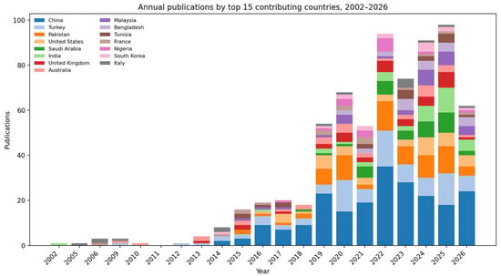
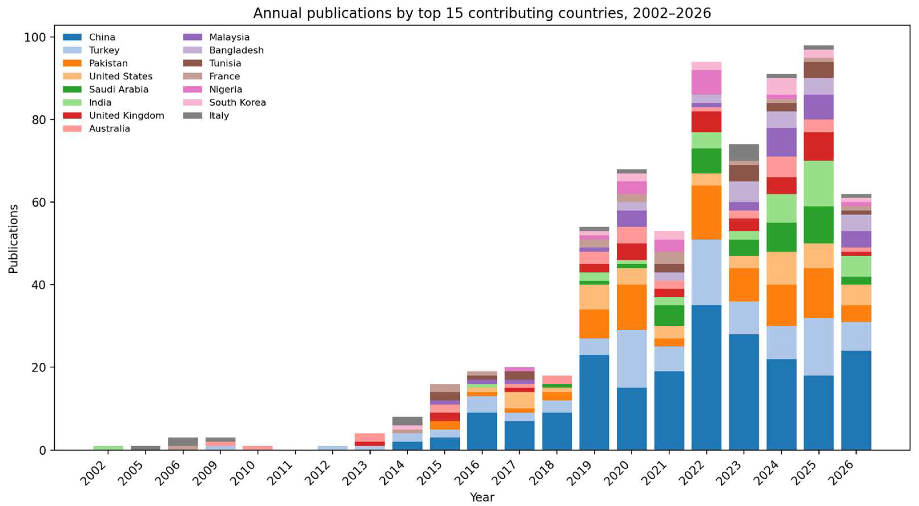
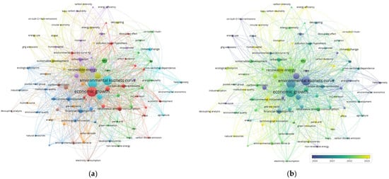
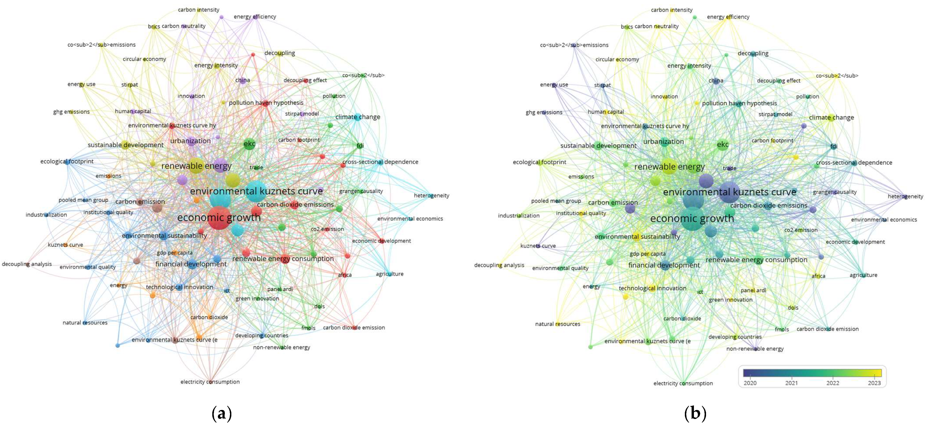
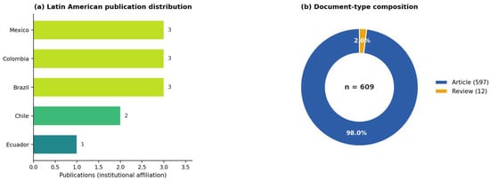
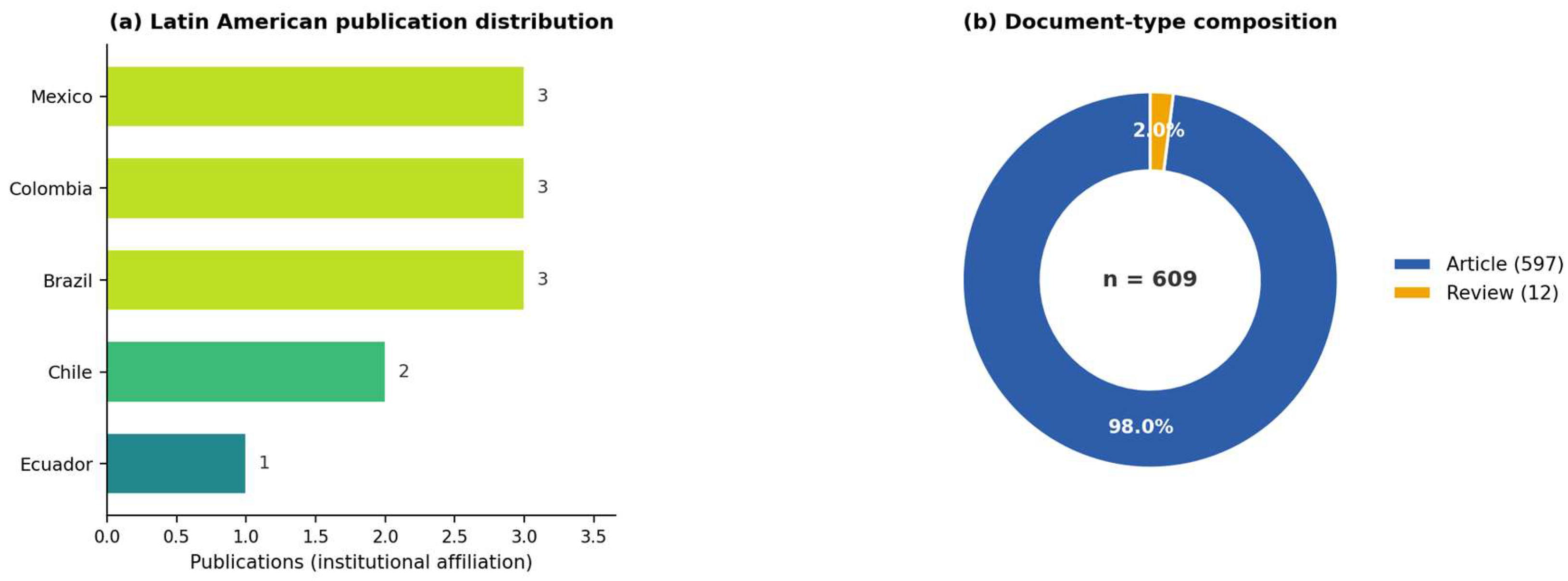
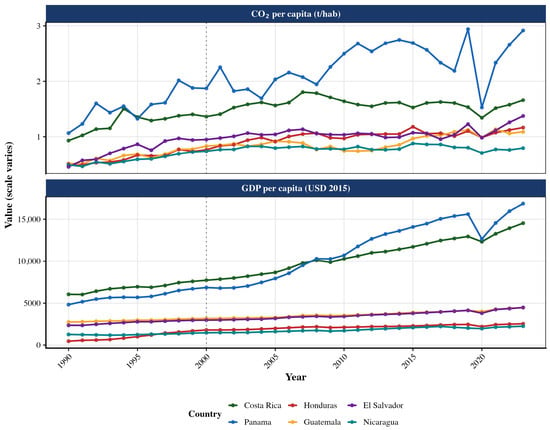
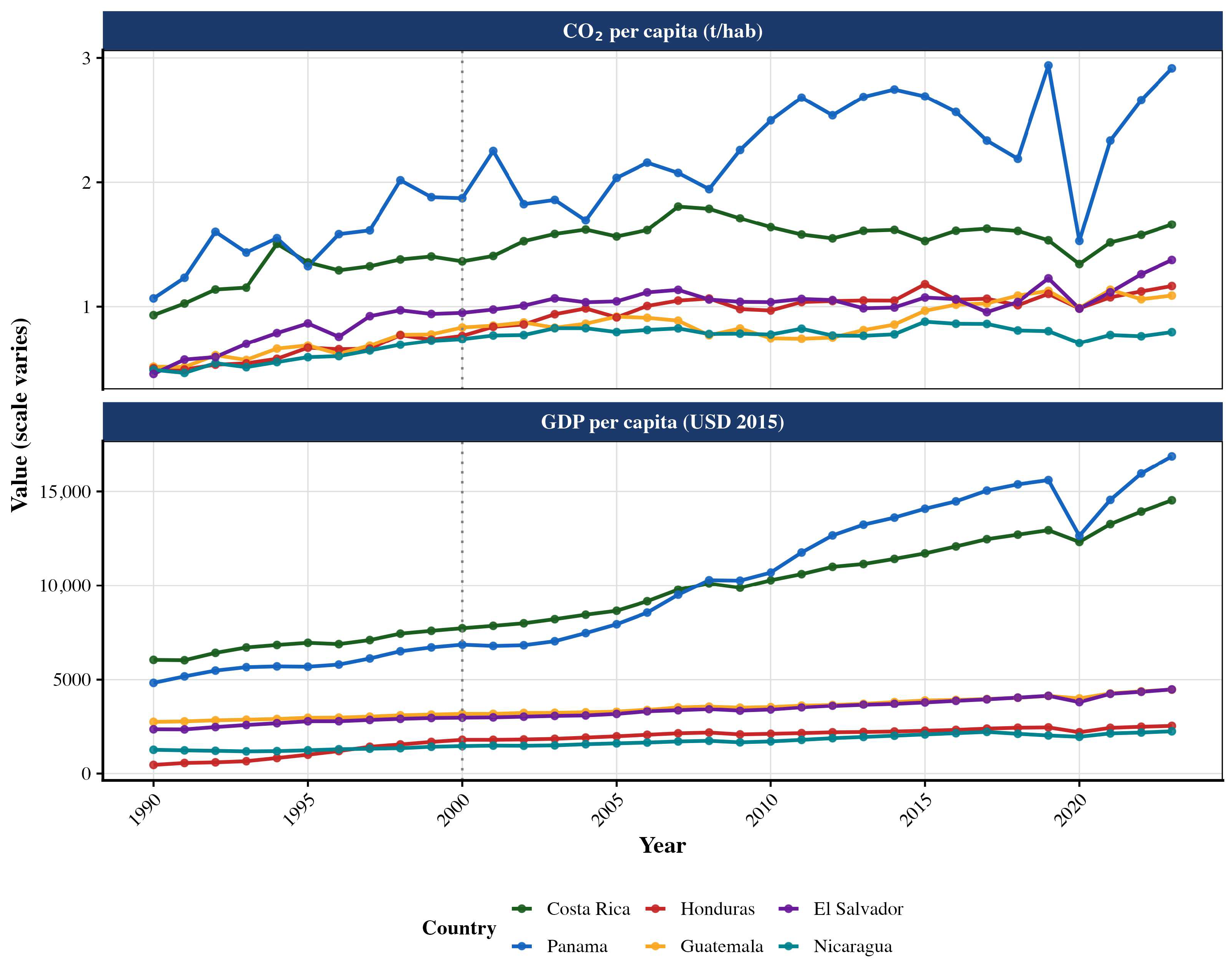
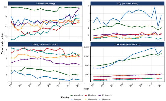
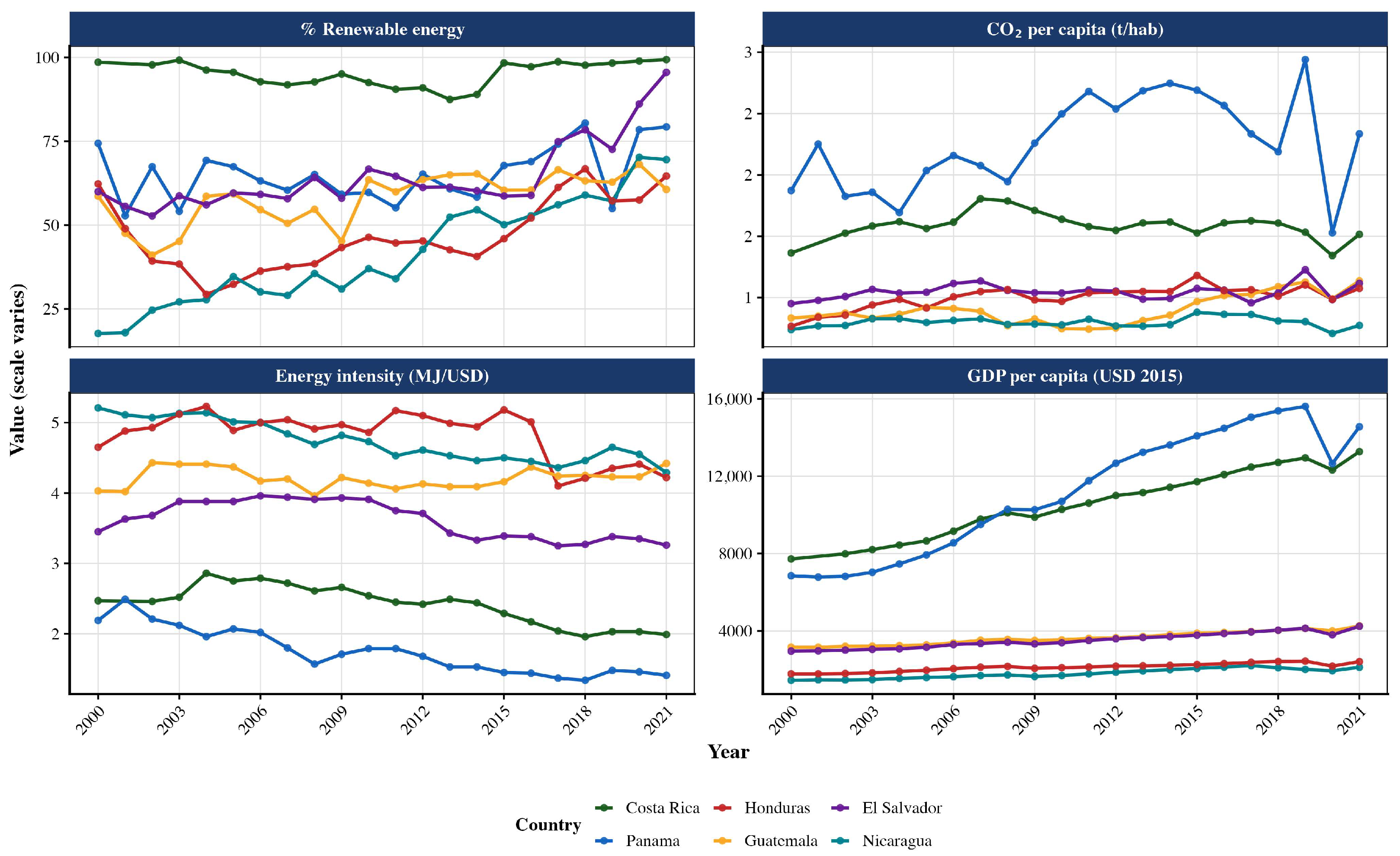
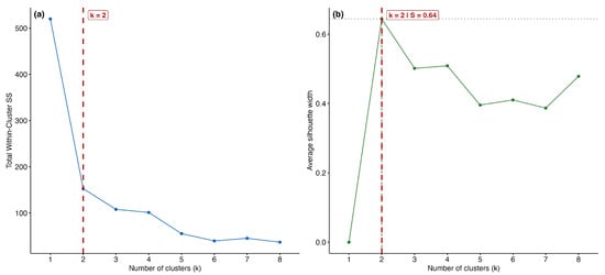
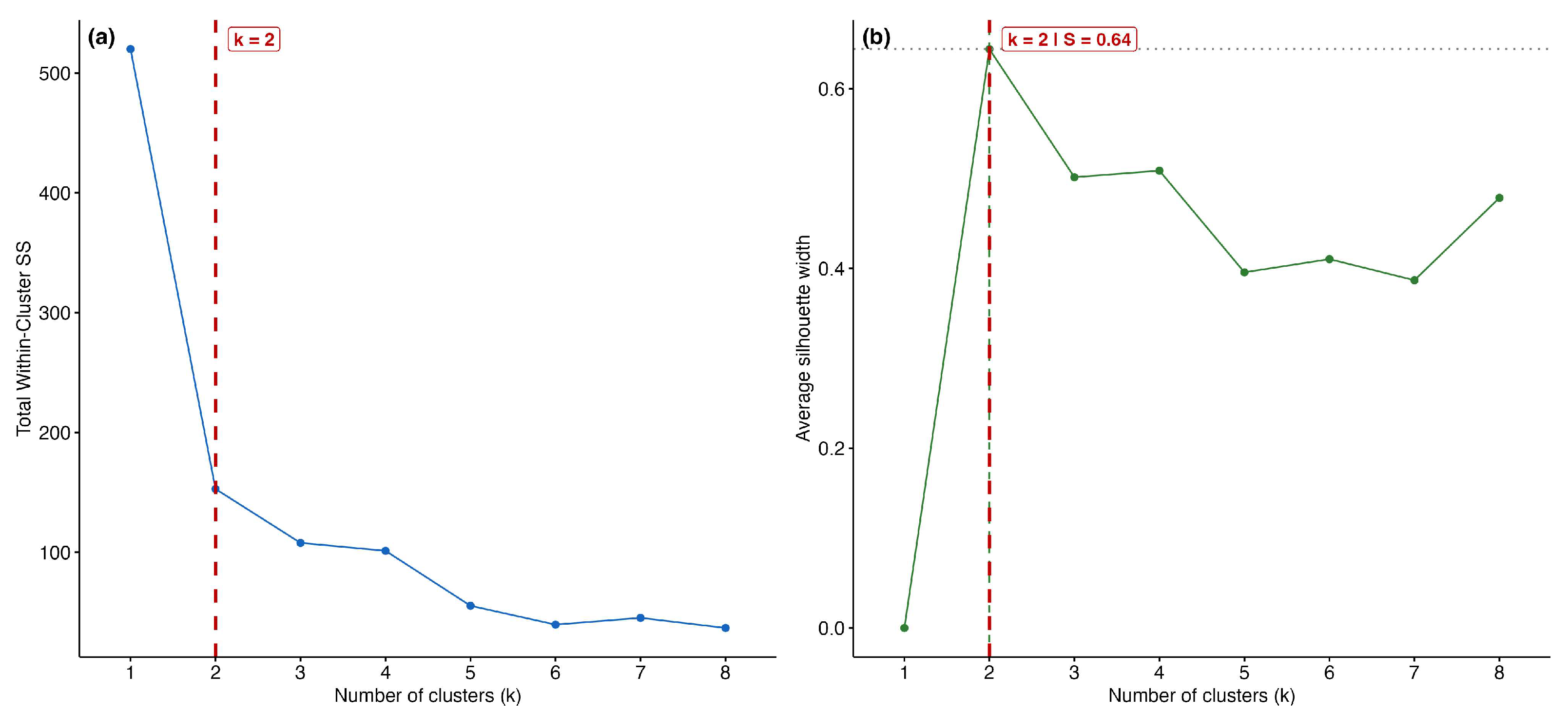
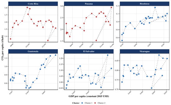
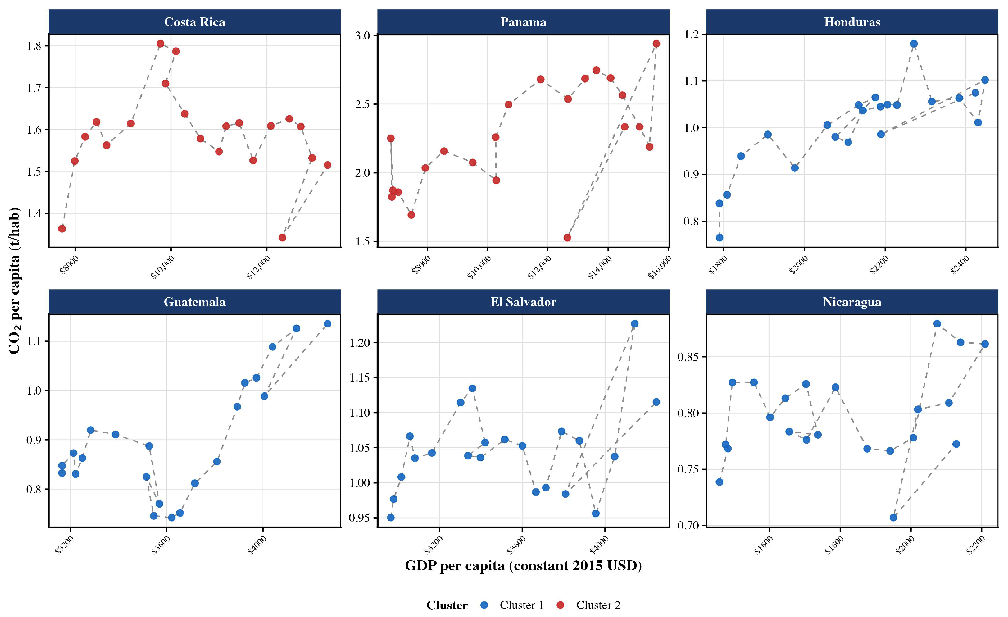
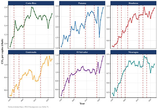
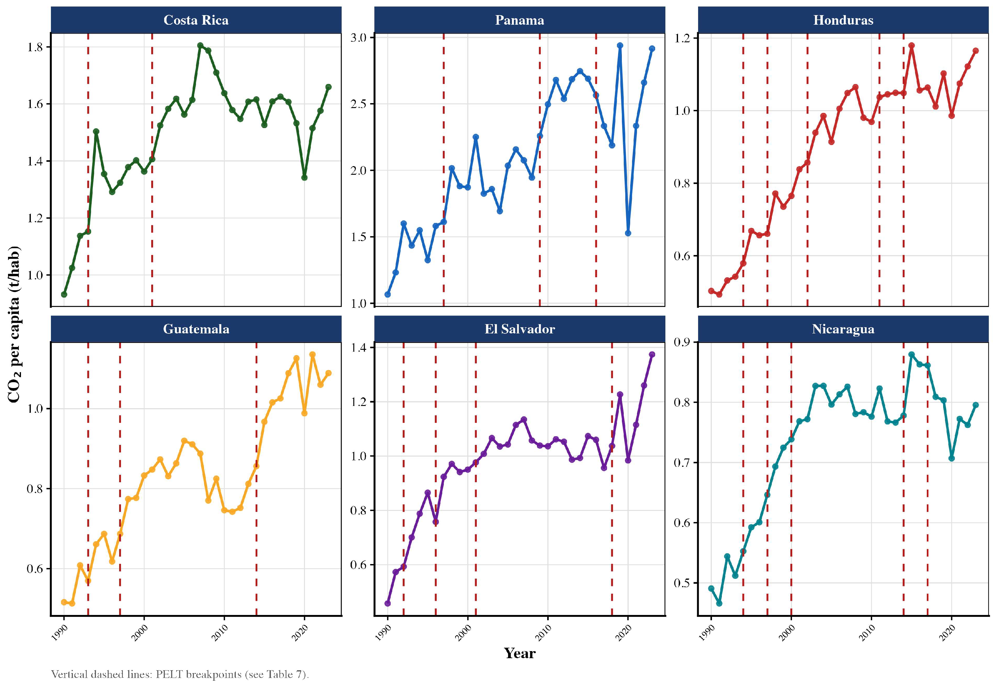
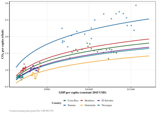
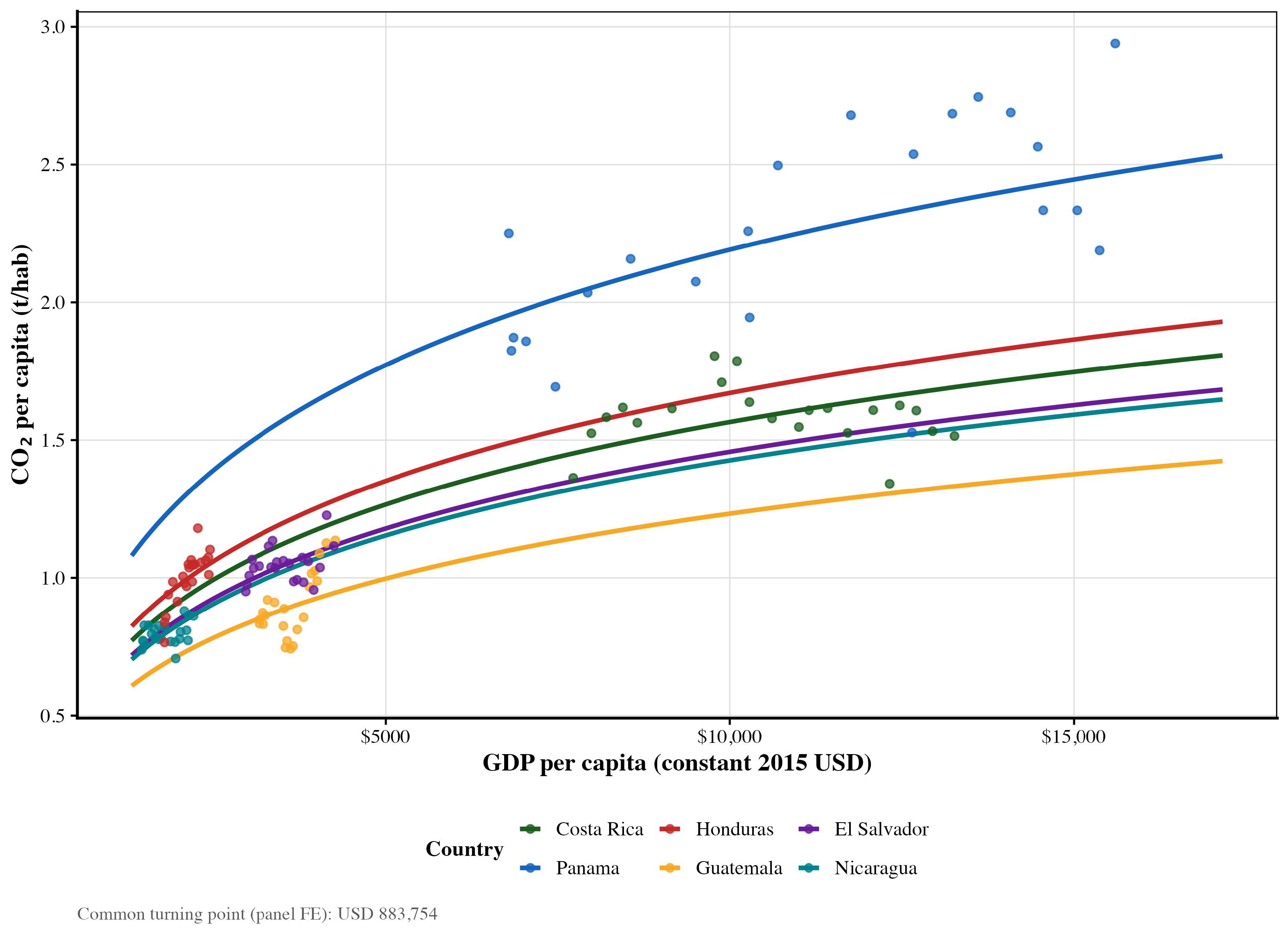
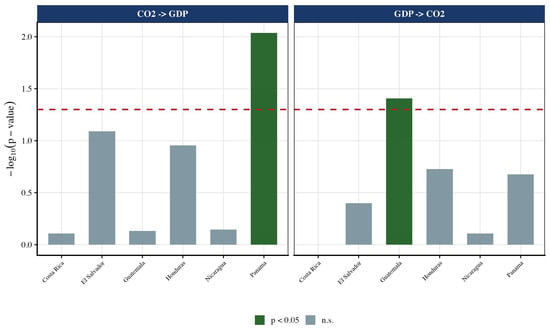
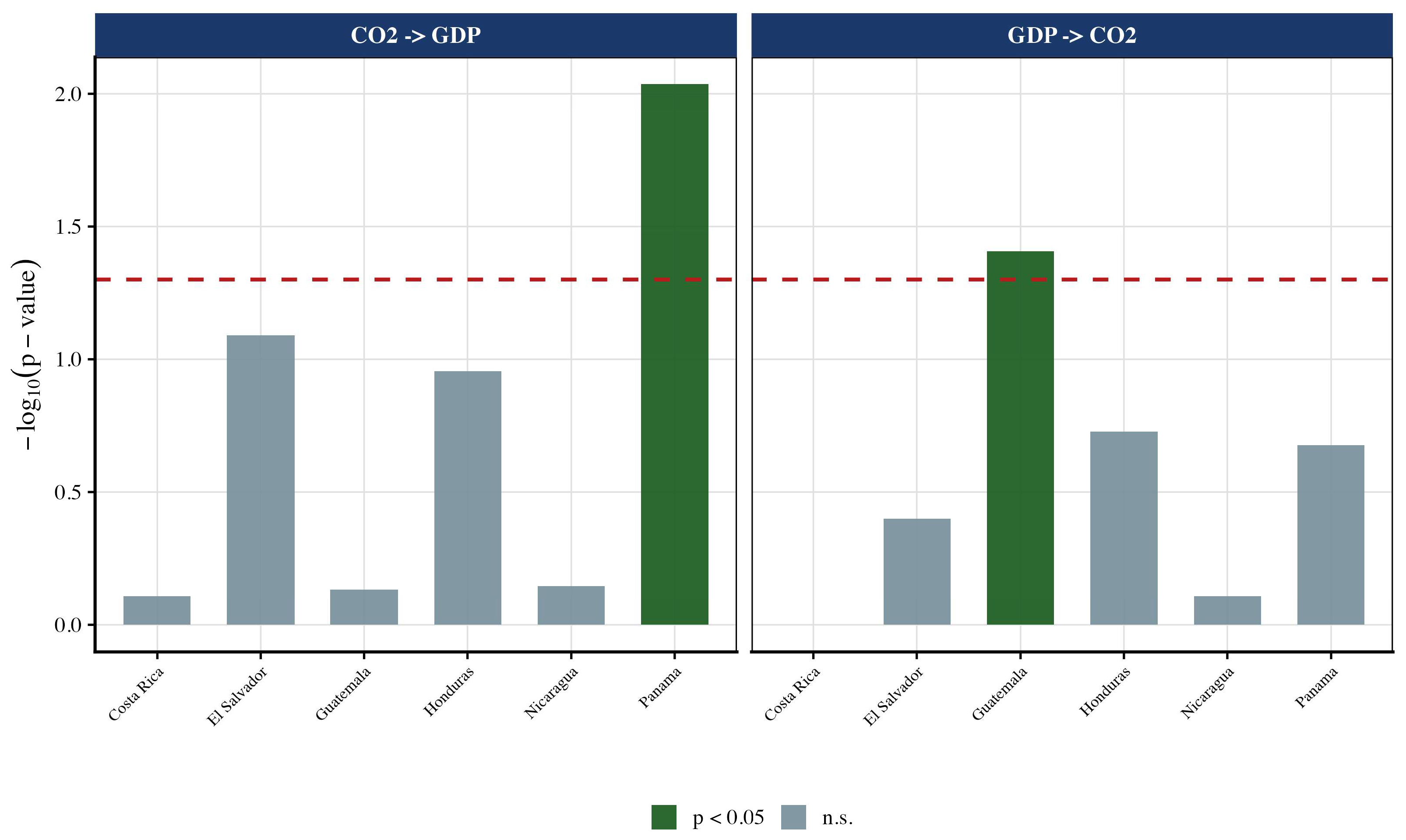
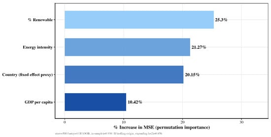
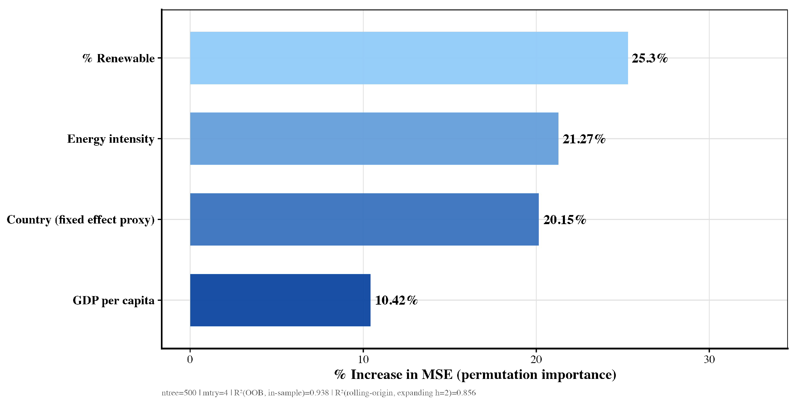
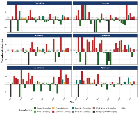
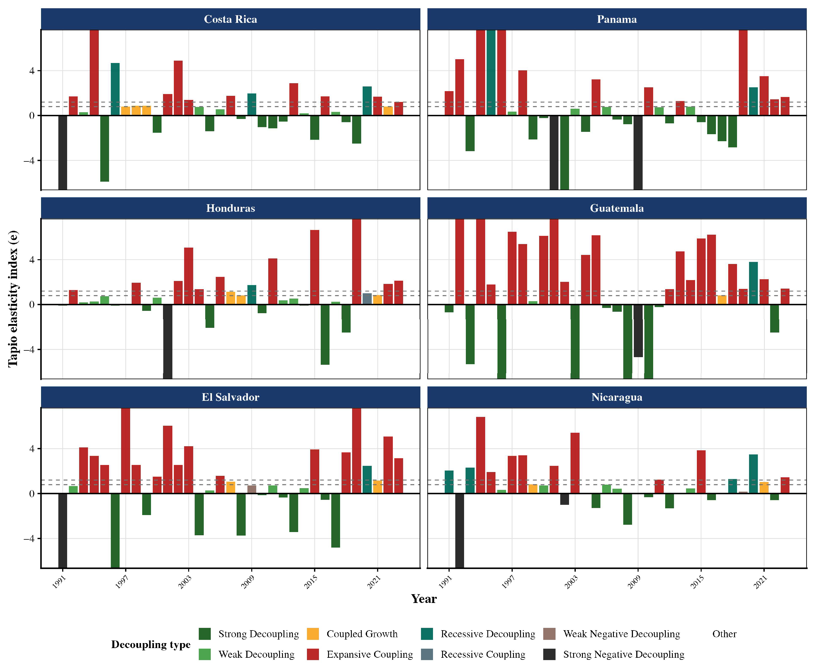
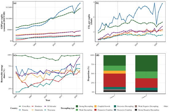
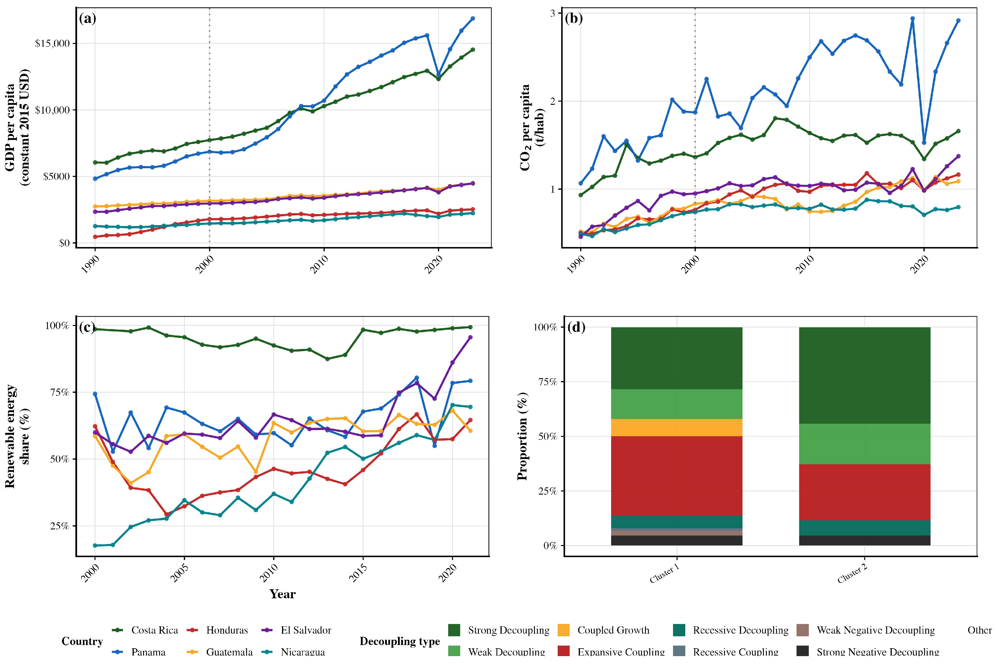
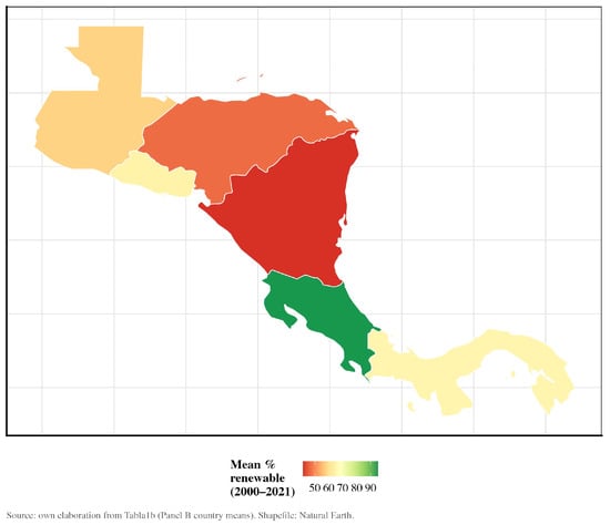
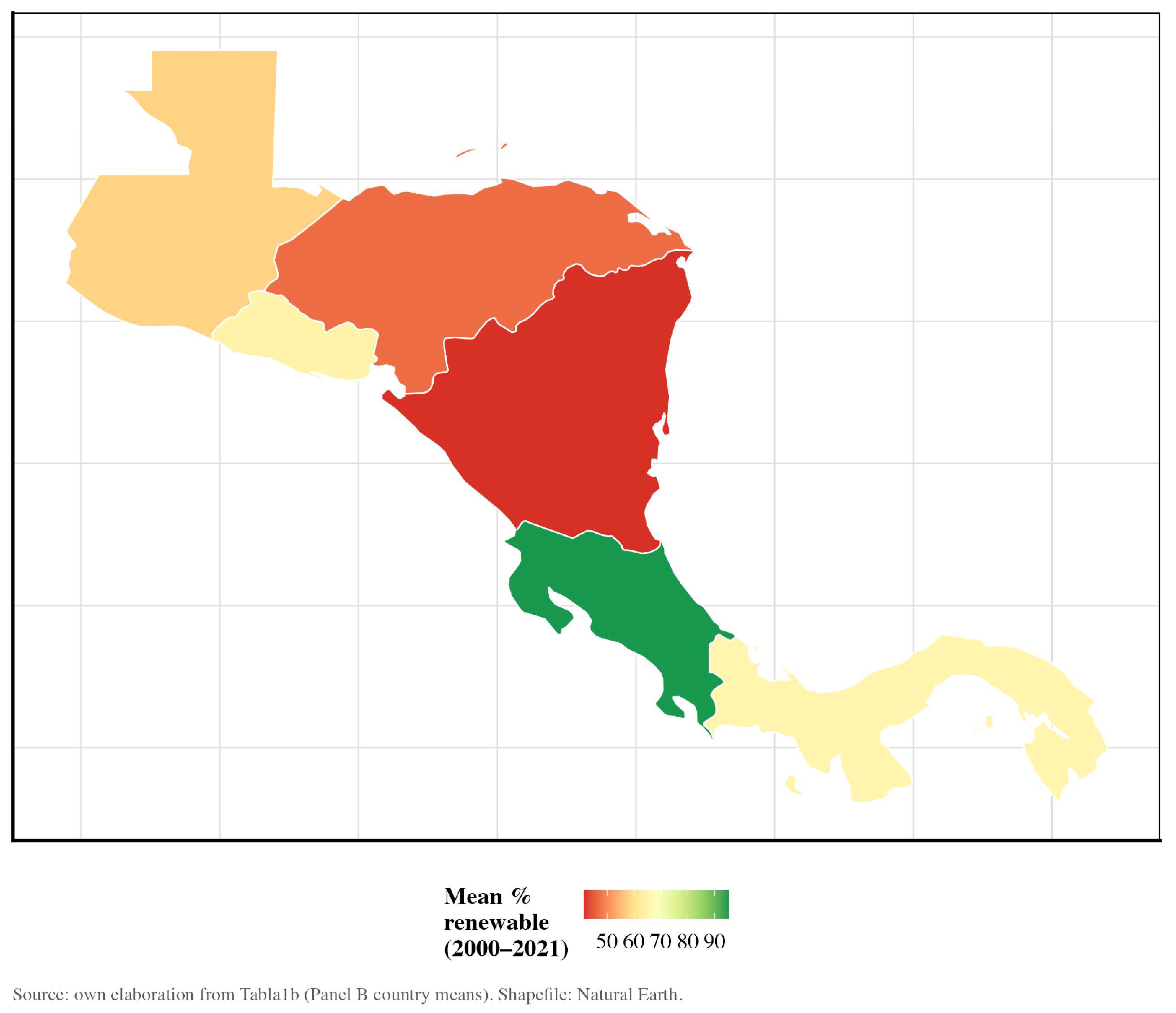

Disclaimer/Publisher’s Note: The statements, opinions and data contained in all publications are solely those of the individual author(s) and contributor(s) and not of MDPI and/or the editor(s). MDPI and/or the editor(s) disclaim responsibility for any injury to people or property resulting from any ideas, methods, instructions or products referred to in the content. |
© 2026 by the authors. Licensee MDPI, Basel, Switzerland. This article is an open access article distributed under the terms and conditions of the Creative Commons Attribution (CC BY) license.