Temporal and Compositional Dynamics of Waste in Tomato Packaging and Its Environmental Footprint: Implications for Agri-Food Sustainability and SDG 12.3

Abstract

This single-plant, single-cycle study characterizes waste dynamics in export tomato packing and quantifies its embedded environmental footprint, contributing to SDG Target 12.3. In total, 196 daily records from six production plants at one Mexican facility were analyzed over an open-field cycle (March–May 2024). Waste composition was analyzed with compositional (long-ratio) methods, and daily magnitude was modeled with four predictive algorithms. Mean waste was 41.4 ± 6.0%, rising steadily across the cycle (+1.8 percentage points per week; 95% CI [1.59, 2.05], robust to serial correlation; r = 0.75). No overall change in waste composition was detected (p = 0.135), and discoloration showed the only positive trend, with no significance after correcting for multiple comparisons (p = 0.159), while equivalence tests were inconclusive for every category. Differences between fields were confounded with their operating windows and could not be separated. With only pre-sort variables, a parsimonious Gradient Boosting model was used to predict daily waste, with R² = 0.846, which is close to the value of 0.898 achieved through the incorporation of same-day grading data. Time-blocked validation showed that neither model outperformed the training mean, indicating interpolation rather than forecasting, with cycle day as the dominant predictor (73% relative importance). Monte Carlo propagation gave a footprint averaging 162 t CO₂eq (90% CI [50, 310]) and 141 million liters of water (90% CI [81, 209]). For the 1127 t discarded, closing the gap between the early and late phases would avoid roughly 21 t CO₂eq and 18 million liters. These findings identify cycle phase as the primary driver of waste and support the use of phase-targeted interventions to reduce both economic loss and environmental impact, contributing to SDGs 2 and 12.

1. Introduction

The tomato (Solanum lycopersicum L.) is Mexico’s leading fruit and vegetable export. In 2024, approximately 3.3 million metric tons were produced, and nearly 2.06 million metric tons were exported, with a value of approximately 3340 million U.S. dollars, consolidating Mexico’s position as the leading supplier to the U.S. market [1]. The state of Sinaloa, in the northwest, accounts for approximately 22% of national production, and together with Sonora, these two states supply more than 80% of all export tomatoes produced during the winter growing season [2]. In the second quarter of 2026, exports totaled US$279M, with the states of Sinaloa (US$110M) and Sonora (US$74.8M) being the highest exporting entities [3].

This context is directly relevant to the following analysis. Given the context of recurring droughts in northwestern Mexico, coupled with water restrictions and anti-dumping duties, reducing losses during the packing stage has become a critical strategy for achieving competitiveness at a lower cost. The severity of this hydrological context merits specification, as it frames the water footprint estimates presented below. During the 2024–2025 cycle, the National Water Commission classified drought across Sinaloa and Sonora as severe to exceptional, storage in the Adolfo López Mateos dam fell to 7.6% of capacity, and close to half of Sinaloa’s cultivable area was left unplanted due to the lack of irrigation water [4,5].

Currently, at packing plants, a considerable portion of the received produce is discarded during the sorting, selection, and grading process due to physical damage, firmness issues, or size specification violations [6,7]. This gives us an idea of the magnitude and importance of developing predictive models to prevent postharvest losses, since beyond the direct loss of the product, this waste represents an inefficient use of water (a scarce resource in the region), energy, and labor invested in production [8]. However, the literature on quantitative predictors of packaging waste is scarce and fragmented, and daily operational records are rarely used for statistical analysis [9].

In this sense, food waste is one of the greatest challenges facing contemporary agri-food sustainability. Worldwide, approximately 931 million metric tons of food is lost or wasted each year throughout the supply chain, with direct consequences for food security, the sustainable use of natural resources, and greenhouse gas emissions [10]. Recognizing the magnitude of this issue, Target 12.3 of the Sustainable Development Goals (SDGs) aims to reduce per capita food waste at the retail and consumer levels by 50% and losses along production and supply chains by 2030 —including those resulting from postharvest handling [11]. It should be noted that progress toward achieving this target is monitored through the Food Loss Index, for which the FAO serves as the custodian agency. More precisely, monitoring relies on indicator 12.3.1, comprising two sub-indicators: 12.3.1 (a), the Food Loss Index, covers losses from postharvest up to but excluding retail and is curated by the FAO, and 12.3.1 (b), the Food Waste Index, is curated by UNEP. The losses examined in this study occur between reception and packing and are therefore captured by sub-indicator 12.3.1 (a).

The importance of studying waste in packaging lies in its significant impact on several SDGs. Within the framework of this research, we contribute directly to SDG 12 (responsible production and consumption); SDG 2 (zero hunger), given the possibility of recovering products suitable for consumption; and SDG 13 (climate action), by avoiding the emissions involved in discarded products. This sustainability perspective implies that waste should not be evaluated solely in terms of its economic cost but also based on its environmental footprint: every kilogram of discarded tomatoes incorporates, in its production, the water, energy, fertilizers, and emissions associated with their cultivation—resources that are irreversibly lost when the fruit does not reach the market [12,13]. In addition, quantifying this footprint is essential for assessing the true cost of waste and for prioritizing mitigation efforts [14].

This study addresses two areas of interest in this field. First, most studies treat waste as an aggregate quantity—that is, without distinguishing between its magnitude (how much is discarded) and its composition (why it is discarded). These two dimensions may behave differently throughout the season. It is likely that waste could increase without a change in its underlying causes, or it could undergo a qualitative shift, even if the overall level remains constant. Distinguishing between these two cases has direct practical implications, as it prompts us to implement interventions aimed at different objectives.

Analyzing the composition of waste also poses a methodological challenge. Since the proportions of the categories must add up to 100%, this is a case of composite data subject to the constant-sum constraint. Therefore, applying ordinary correlation or regression to these proportions generates strong but fictitious or spurious correlations: If one category gains weight, at least one other category must lose it, regardless of the underlying process [15,16]. The proposed solution consists of working with log-ratio transformations, which free the data from this constraint and allow standard methods to be applied validly.

Second, recent research on postharvest losses points to predictive models as the most promising direction, particularly machine learning methods capable of capturing nonlinear relationships and forecasting the magnitude of losses based on operational data [14,17]. These studies, however, typically evaluate models with randomly partitioned cross-validation on data that are implicitly time-ordered, and they treat multi-category loss records as independent proportions rather than as a constrained composition. Neither practice is specific to tomato packing, but both are common across the postharvest loss literature, and each can produce misleading conclusions. Random portioning of correlated daily records overstates forecasting ability, and uncorrected proportions generate correlations that are artifacts of the summation constraint rather than of the underlying process. Prior tomato-packing-loss studies report on predictor associations and loss magnitudes but do not, to the best of our knowledge, test whether their validation scheme leaks temporal information or evaluate their compositional results through a summation-constraint-free analysis. This study was designed explicitly to address both issues using operational data from a working plant, addressing this gap in the literature.

The overall objective of this work was to characterize the temporal and compositional dynamics of waste across six production fields—all of which are processed at the same plant—to build a predictive model of its daily magnitude and subsequently quantify its embedded environmental footprint as a basis for assessing its sustainability. The specific study objectives were the following: (1) to quantify, throughout the cycle, the temporal trend in the magnitude of waste; (2) to determine, through compositional analysis, whether the waste structure causes changes as the season progresses; (3) to assess whether differences between farms are independent of the harvest time; (4) to compare the performance of predictive models and identify the most informative variables; and (5) within the framework of SDG Target 12.3, to estimate the embedded carbon and water footprints of the wasted product and its mitigation potential.

Two hypotheses are proposed. H1 is that the magnitude of waste increases throughout the production cycle, reflecting the increase in raw material waste. This expectation has a physiological basis. As the growing season progresses from March to May in an arid region, ambient temperatures rise, and plants experience heat stress, which accelerates fruit senescence, impairs firmness retention, and reduces the quality of the raw material reaching the packing line [6,7]. Field-level temperature, radiation, and cultivar and harvest maturity lie outside the packing records analyzed here, so the hypothesis is framed at the level of the seasonal gradient itself. H2 is that waste composition remains relatively stable by cause, such that season progression has a greater impact on the amount of waste than on the predominant loss type.

2. Materials and Methods

2.1. Data

Daily operational records from a tomato packing plant in northwestern Mexico were used, corresponding to the production cycle from 7 March to 7 May 2024 (61 calendar days). Raw operational data were recorded and maintained in Microsoft Excel (Microsoft 365). All analyses were performed on a 15-inch MacBook Air (Aple M4 chip). Statistical modeling and figure generation used Python 3.12.3 with SciPy 1.17.1, NumPy 2.4.4, pandas 3.0.2, scikit-learn 1.8.0, statsmodels 0.14.5, matplotlib 3.9.1. and Claude Sonnet 5, To transform matplotlib output graphs into high-quality vector graphics and to improve their resolution.

Each record corresponds to a complete daily batch from one of six open-field production fields (coded M 1-1, M 1-2, M 2-1, M 3-3, R 2-2, and C-2-2). After excluding records with no product received, the analytical dataset comprised 196 active observations spread over 59 operating days. The raw register contained 208 field-by-day rows covering every combination of field and calendar date; rows were retained only when recorded reception exceeded zero, since a zero denotes that the field did not deliver on that date and the waste percentage is therefore undefined rather than null. This criterion removed 112 rows. Consistency was then verified by checking that the packed plus discarded kilograms did not exceed kilograms received and that the seven waste categories were summed to the reported total, within rounding tolerance. No record failed these checks, and no imputation was performed. Across the six fields, the number of records ranges from 11 (M 3-3) to 49 (M 2-2) days (Table 1). Every one of the 59 operating days involved between two and five fields processed simultaneously (8 days with two fields, 30 with three, 15 with four, and 6 with five), so the dataset has a panel structure—fields nested within days—rather than that of independent, single-field daily time series. For each record, the following values were considered: volume received and packed, total waste, classification of the packed product by quality grade (grades 1, 2, and 3), and commercial size (jumbo, XL, L, M, national). In addition, waste was broken down into seven categories: discolored, blotchy ripening, mechanical damage, firmness issue, misshapen, undersized, and small. Quality grade, commercial size, and waste category were assessed in a single daily sorting pass at the end of each batch. Therefore, these three variable sets become available simultaneously with the waste outcome itself, not before; volume received is the only predictor known at intake, ahead of sorting.

Table 1. Profile of the producing fields and their operating window within the cycle.

Producing Field	n (Days)	M ± SD (%)	Min–Max (%)	Volume Share (%)	Operating Window
M 3-3	11	48.4 ± 5.4	42.9–58.0	5.9	Days 50–61 (late only)
M 2-1	24	43.3 ± 4.9	35.6–55.5	18.8	Days 22–59 (2nd half)
M 1–2	49	41.0 ± 5.5	32.9–58.0	25.0	Days 0–60 (entire cycle)
C-2-2	31	41.0 ± 6.0	30.9–58.1	12.4	Days 0–60 (entire cycle)
R 2-2	33	40.7 ± 5.9	30.9–58.1	12.4	Days 0–60 (entire cycle)
M 1-1	48	40.1 ± 6.3	17.3–56.0	25.5	Days 1–61 (entire cycle)

M = mean; SD = standard deviation; n = number of operating days. The operating window highlights the structural confounding between field and time: fields M 3-3 and M 2-1 operated only during advanced stages of the cycle, leaving no period in which all six fields were jointly observed.

The main response variable was the percentage of waste, defined as the ratio of kilograms discarded to kilograms received. Time was coded as the number of days elapsed since the start of the cycle (day 0 = March 7). Therefore, cycle day operates as a temporal proxy: it aggregates every seasonal factor co-varying with season progression—field condition, harvest maturity, plant age, ambient temperature—which the packing records do not resolve individually. Daily records were also not statistically independent. Batches from the same field from close dates share growing conditions, and the series as a whole follows the seasonal gradient described in Section 3.1. This dependence is addressed directly in the inferential procedures below rather than assumed away.

2.2. Analysis of the Magnitude and Field–Time Confounding

The temporal trend in the magnitude of waste was evaluated using linear regression on the cycle day, reporting the slope with its 95% confidence interval. Because daily records are serially dependent, ordinary least-squares standard errors—which assume independent errors were supplemented with two robustness checks: heteroskedasticity- and autocorrelation-consistent (HAC, Newey-West, 3 lags) standard error, standard error, and standard errors clustered by production field. Residual autocorrelation was inspected using the Durbin–Watson statistic and lag-1 to lag-3 sample autocorrelations. Differences between fields were tested using one-way ANOVA and the nonparametric Kruskal–Wallis test, complemented by Levene’s test for homogeneity of variances and Welch’s ANOVA, which does not assume equal variances across fields. To assess whether the field effect was independent of time, the explained variance was decomposed using nested models: field only, day only, and both. The unique contribution of each factor was calculated as the increase in R² when added to a model that already contained the other factor, and the shared component as the difference between the sum of marginal R² values and that of the full model.

2.3. Compositional Data Analysis (CoDA)

At this stage, the decision was made to consider the seven waste categories (discoloration, blotchy ripening, mechanical damage, firmness issue, misshapen, undersized, and small), the proportions of which sum to unity. To avoid biases arising from the constant-sum constraint, the centered log-ratio (CLR) transformation was applied, which expresses each component as the logarithm of its ratio to the geometric mean of the vector [15]. None of the 196 records contained a zero count in any category, so no zero-replacement procedure was required before the log-ratio transformation. Standard multiplicative replacement could be applied if zeros were present in future extensions of this dataset. Using the CLR coordinates, the temporal trend for each category was evaluated via regression against the cycle day. Since this involves seven simultaneous univariate contrasts, p-values were corrected using the Benjamini–Hochberg false discovery rate, and significance was judged on the corrected scale. Because a non-significant trend does not by itself establish stability, the two one-sided tests (TOST) approach was additionally applied to each category so each category could be positively classified as stable, changing, or inconclusive rather than only as not significant. The equivalence margin followed the smallest conventional effect-size threshold (Cohen’s d = 0.2) rather than a wider one. In the TOST framework, equivalence bounds are ideally derived from a smallest effect size of interest specific to the research context. Where no discipline-specific benchmark exists, as is the case for compositional waste data, Cohen’s conventional thresholds provide an accepted default [18,19]. Among these, d = 0.2 is the strictest: wider bounds make equivalence easy to declare, since most real-world effects are small to medium in magnitude [19], whereas the smallest threshold requires the true change to be very small before equivalence can be confirmed. Similarly, the overall compositional change was tested using a multivariate permutation test (5000 iterations), which allows for the evaluation of the maximum canonical correlation between the set of CLR coordinates and time, providing a p-value free of distributional assumptions. Because the observations are time-ordered, this test was repeated using block permutation (contiguous 5-day blocks shuffled as units rather than individual days), thereby preserving the short-range temporal structure under the null hypothesis and providing a check against the permutation-free result.

2.4. Predictive Models

Four models were compared to predict the daily waste percentage: (i) multiple linear regression, (ii) Ridge regression, (iii) Random Forest, and (iv) Gradient Boosting. Two predictor sets were evaluated in parallel. The full set included the cycle day, the volume received, the proportions of quality grades 2 and 3, and the commercial sizes. As noted in Section 2.1, the grade and size variables are only viable once the same-day sorting pass is complete, so this set describes waste once the produce has been discarded and not beforehand. A second, pre-sort set retains only the cycle day and volume received—the two quantities known before sorting—to assess how much predictive value depends on variables that cannot support operational early-warning applications. Given the desire for a more generalizable model, field indicator variables were deliberately excluded from the final set of predictors to avoid multicollinearity and overfitting; a sensitivity test confirmed that their removal left the predictive performance unchanged or marginally improved it (the R² for Gradient Boosting increased from 0.895 to 0.898). Hyperparameters were fixed a priori rather than tuned, so that the limited sample was not used up in a search procedure. They were chosen to keep model capacity low relative to n = 196. Gradient Boosting used n_estimators = 200, max_depth = 3, and learning rate = 0.1. Random Forest used n_estimators = 300 and max_depth = 8, and Ridge regression used alpha = 1.0. A maximum depth of three restricted each boosting stage to shallow interactions, which is the principal safeguard against overfitting at this sample size. Cross-Validated performance is consistent with this choice: R2 for the pre-sort Gradient Boosting model plateaus at n_estimators = 200 (R² = 0.846) and declines slightly beyond it (R² = 0.854 at 300; 0.844 at 500), while max depth = 3 outperforms both shallower settings (R² = 0.52, SD = 0.56, at depth 8). Random Forest’s performance was similarly insensitive to n_estimators beyond 100—300. All models used random_state = 42. Performance was evaluated using five-fold cross-validation, reporting the average coefficient of determination (R²) and its standard deviation, together with the root mean squared error (RMSE) in percentage points of waste, interpretable against the standard deviation of the response (6.02 pp), the mean absolute error (MAE), fold-level results, and an empirical 95% prediction interval derived from the distribution of cross-validated residuals. Because adjacent dates are correlated, performance was also assessed under five-fold cross-validation blocked by contiguous time segments, where each test fold covers a stretch of the cycle absent from training. The two schemes answer different questions: random partitioning measures reconstruction within the observed cycle, blocked partitioning measures extension to periods the model has not seen before. Likewise, the relative importance of the predictors was obtained from the best-performing model—reported here as the model’s internal split gain importance, a measure of relative predictive contribution rather than of variance explained.

2.5. Estimation of the Environmental Footprint

The environmental footprint of the product discarded and classified as waste was estimated by multiplying the kilograms discarded by life cycle assessment (LCA) impact factors reported for the production of fresh tomatoes in open fields. To mitigate geographic bias, specific ranges of factors were selected primarily for open-field production on irrigated land in warm, arid regions. For the carbon footprint, a central factor of 0.080 kg CO₂eq per kilogram was used (median for open-field systems; range: 0.010–0.340), consistent with a recent systematic review of 50 LCA studies [20]. For the water footprint, a central factor of 110 L per kilogram (range: 50–214) was used, appropriate for irrigated open-field production in arid regions [21]. The system boundary is cradle-to-farm-gate. It covers agricultural production only—inputs, field operations, and on-farm irrigation—and excludes packing plant energy and water use, transport, and the disposal or treatment of the discarded fruit itself, none of which was characterized in the source studies. No co-product allocation was required, since fresh tomato is the sole product of the modeled system. Waste was considered to embody the full upstream footprint of its production, with no credit or burden assigned for its eventual disposal fate (landfill, compost, or animal feed), which was not recorded by the plant and therefore not modeled. The water metric is a volumetric footprint (blue plus green water), not a scarcity-weighted indicator. In a region with documented water stress, as described in Section 1, a scarcity-weighted metric (e.g., AWARE characterization factors) would likely value this water more heavily than the volumetric figures reported here, and this is noted as a limitation of our study. These intervals are wide relative to the differences the analysis characterizes. Rather than combine a single central coefficient with a separately stated range, uncertainty was propagated formally: 20,000 Monte Carlo draws were taken from triangular distributions over each factor’s reported minimum, mode, and maximum and applied to the discarded tonnage to obtain a distribution of the total footprint, summarized by its mean and 90% interval (5th–95th percentile). To measure the mitigation potential, the calculation of the avoidable footprint is considered if end-of-life waste was reduced to initial-phase levels, while keeping the processed volume constant. The figure quantifies the footprint associated with an observed gap, and the feasibility of closing that gap is a separate question. The same Monte Carlo procedure was applied to this avoided quantity. These were deliberately first-order approximations intended to gauge the order of magnitude of the impact, not site-specific life cycle inventories. It is important to note that the highly mechanized export packaging practices in northwestern Mexico may differ from the factors identified in the literature, so it is suggested that the absolute values be interpreted as indicative ranges rather than precise, generalizable figures.

3. Results

3.1. The Magnitude of Waste Increases Throughout the Cycle

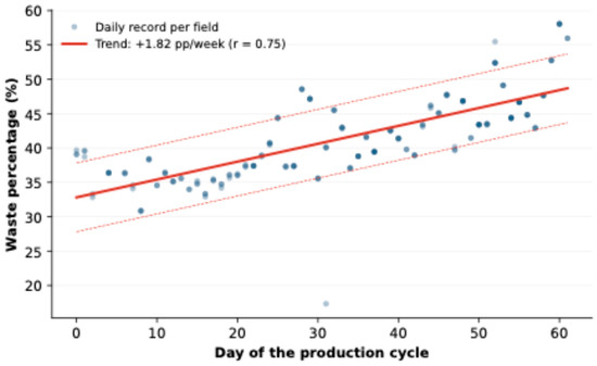
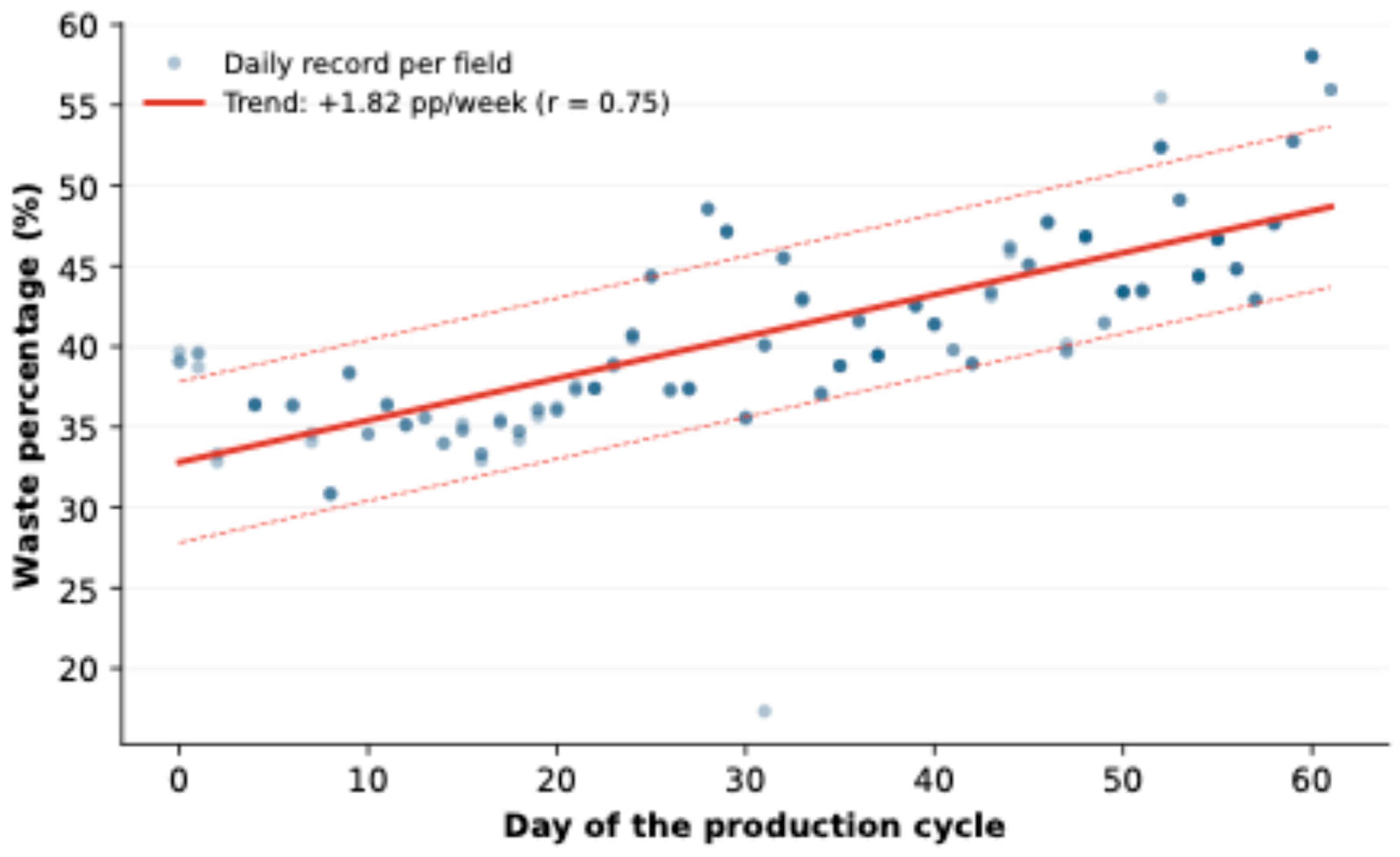
During the study period, 2,663,895 kg of tomatoes were processed. An average of 41.4% (SD = 6.0%; range: 17.3–58.1%) of this quantity was recorded as waste. A strong upward trend over time was detected, indicating that waste increased at a rate of 1.8 percentage points per week (95% CI [1.59, 2.05], equivalently 0.260 pp per day, 95% CI [0.228, 0.293]; r = 0.75, p < 0.001), rising from levels close to 30% at the beginning of the cycle to over 50% at the end (Figure 1). This trend alone explained 56% of the variance in daily waste, confirming hypothesis H1. Because daily records are serially dependent (Durbin–Watson = 0.60; lag-1 residual autocorrelation = 0.70), the ordinary least-squares confidence interval above understates the true uncertainty. Under Newey–West standard errors, the interval widens to [0.20, 0.32] pp per day and remains highly significant (p = 5.5 × 10⁻¹⁸); standard errors clustered by field give an even narrower interval ([0.24, 028]). The direction and approximate magnitude of the trend are therefore robust to the choice of standard error, though the OLS interval reported above should be read as optimistic.

Figure 1. Evolution of waste percentage throughout the production cycle. Each data point represents a daily batch from a production field; the fitted line shows the linear trend. Waste increases steadily as the season progresses (r = 0.75, p < 0.001).

3.2. Differences Among Production Fields Are Not Discernible over Time

When differences in waste were evaluated, the six fields differed in their average waste (ANOVA: F [5, 190] = 4.45, p < 0.001; Kruskal–Wallis: H = 18.6, p = 0.002); variances were homogeneous across fields (Levene’s test: p = 0.94), and Welch’s ANOVA, which does not assume this, gave a consistent result (F [5, 61.5] = 4.73, p = 0.001), with M 3-3 at the top (48.4%) and M 1-1 at the bottom (40.1%). However, as shown in Table 1, the fields operated during different time windows. M 3-3 reported operations only during the last eleven days of the cycle, and M 2-1 during its second half, while the other fields operated throughout the entire season. M 3-3 provides the clearest illustration of the problem this creates; its entire operating record falls in the last quintile of the cycle, the same stretch in which every field’s waste is highest, so its elevated average cannot be attributed to the field as such without also attributing it to the occurrence of operation in this field.

Variance decomposition confirmed that the apparent effect of the field is, for the most part, a masked temporal effect. The day of the cycle contributed 46.2 percentage points of R² above the field, while the field contributed only 0.7 percentage points above the day. The full model containing both terms reaches R² = 0.567, compared to 0.560 with the day alone and 0.105 with the field alone, with a shared component of 9.8 percentage points. When controlling for the processing time, no field differed significantly from the others (all coefficients p > 0.22). Consequently, the originating field and phase of the cycle cannot be separated in these data. Two fields operated only in advanced phases, so no period exists in which all six were jointly observed, and what appears as an origin effect is indistinguishable from the processing time. Whether the fields differ agronomically is a question this design leaves for future work.

3.3. The Composition of the Waste Remains Stable Regardless of Time

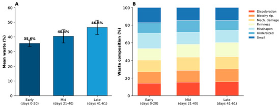
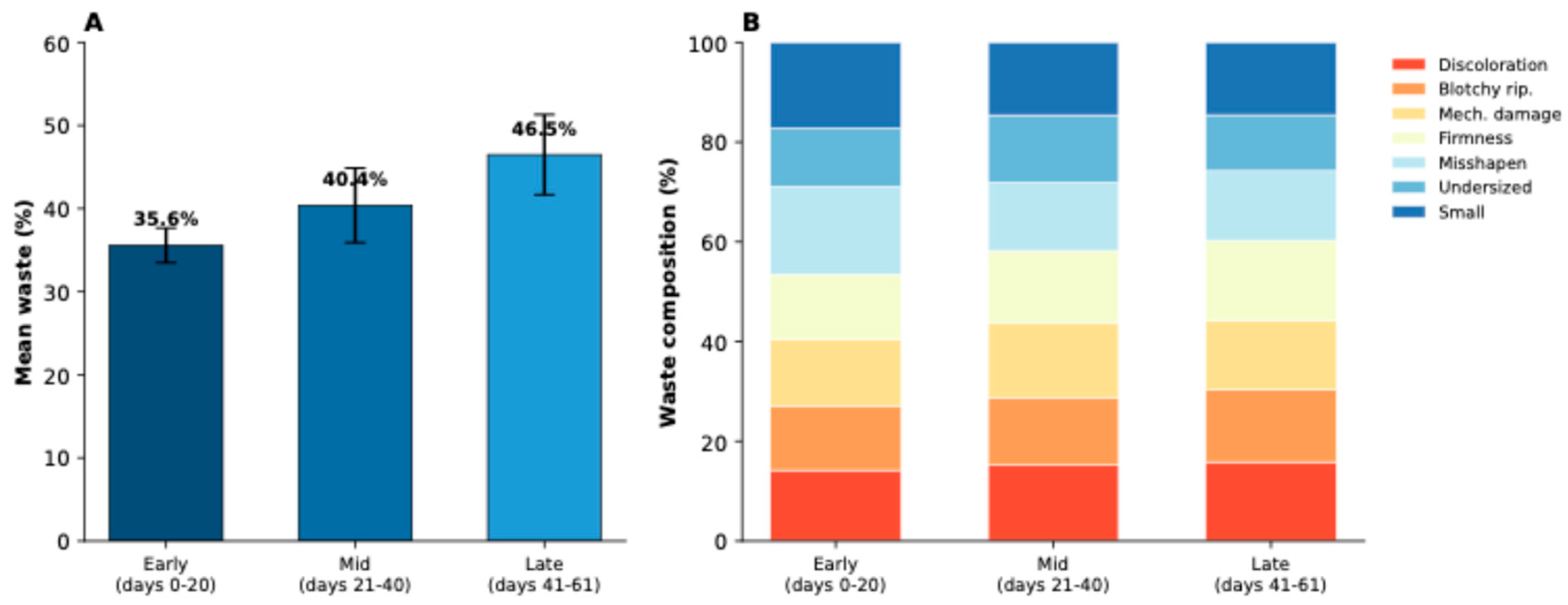
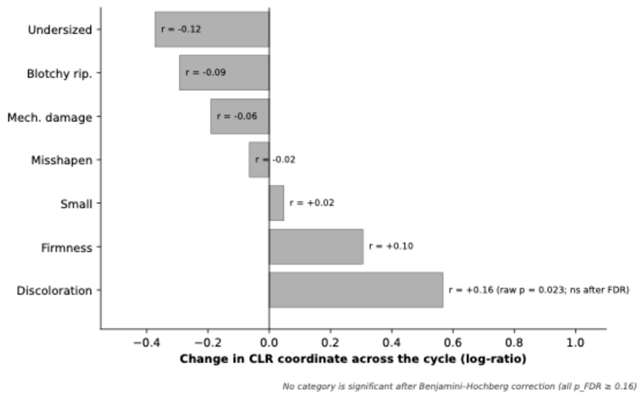
Compositional analysis revealed this study’s key finding. While the magnitude of waste shows marked growth, no change in its composition by cause was detected across the cycle, and equivalence testing could not positively confirm stability (Figure 2). The multivariate permutation test did not detect a significant overall change in composition (canonical correlation = 0.22; p = 0.135); repeating the test with a contiguous 5-day block permuted as units, to preserve the short-range temporal structure, gave a consistent result (p = 0.168). In this regard, of the seven categories, only “discoloration” (referred to by local producers as “clown-faced”) significantly increased its relative weight as the season progressed (r = +0.16; p = 0.023); the remaining six categories showed no significant temporal change (Table 2, Figure 3). When corrected for the seven simultaneous contrasts, this value increases to p = 0.159, so the discoloration trend is best read as exploratory and warrants targeted measurement in future cycles. The two one-sided equivalence tests (TOST) approach was used against a small-effect margin (Cohen’s d = 0.2), the results of which were inconclusive for all seven categories, including discoloration (the largest observed effect, d = 0.57). The data neither confirm a change large enough to matter operationally nor rule one out. The compositional result is therefore an absence of detected change, not a demonstrated stability, and is reported as such throughout this paper. This pattern confirms Hypothesis H2. The progression of the cycle alters the amount of waste, but not the structure of why waste occurs.

Figure 2. Dissociation between the quantity and composition of waste by seasonal phase. Panel (A) shows the average waste (±1 SD) in the initial, middle, and final phases; the magnitude increases steadily. Panel (B) shows the relative composition by cause category as crude percentages, presented in this manner for direct interpretability. The formal compositional test, free from the summation constraint, is shown on CLR coordinates in Figure 3 and confirms the visual stability (no category shows a significant temporal change).

Table 2. Temporal trend of each waste category on CLR coordinates, corrected for multiple comparisons.

Waste Category	CLR Slope	r	p	p (FDR)	Seasonal Trend
Discolored	+0.0093	+0.16	0.023	0.159	Increases (not significant after correction)
Firmness	+0.0050	+0.10	0.151	0.340	No significant change detected
Small	+0.0008	+0.02	0.820	0.820	No significant change detected
Misshapen	−0.0011	−0.02	0.790	0.820	No significant change detected
Mechanical damage	−0.0031	−0.06	0.408	0.572	No significant change detected
Blotchy ripening	−0.0048	−0.09	0.194	0.340	No significant change detected
Undersized	−0.0061	−0.12	0.100	0.340	No significant change detected

CLR = centered log ratio. The slope and correlation (r) correspond to the regression of each CLR coordinate on the day of the cycle. p (FDR) = Benjamini–Hochberg-corrected value across the seven simultaneous contrasts; no category retains significance after correction. The global multivariate test (permutation, 5000 iterations) yielded a canonical correlation of 0.22 (p = 0.135), which was not significant; block permutation (5-day blocks) gave a consistent result (p = 0.168), and TOST equivalence tests were inconclusive for every category.

Figure 3. Change in the relative weight of each waste category throughout the cycle, plotted on centered log-ratio (CLR) coordinates. All bars are shown in neutral gray because no category reaches significance after Benjamini–Hochberg correction. Discoloration, the category with the lowest raw p-value (p = 0.023), is annotated for reference but is not significant on the scale (p = 0.159).

3.4. Prediction of Waste by Cycle Day

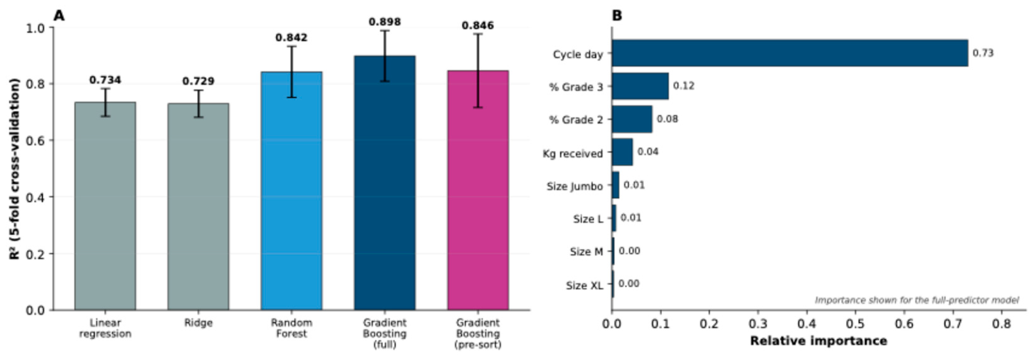
In this part of the analysis, the four models predicted an increasing trend in daily waste as complexity increased (Table 3, Figure 4A). The linear models achieved an R² of approximately 0.73 in cross-validation, while the ensemble methods outperformed them. Random Forest achieved an R² = 0.842 and that of Gradient Boosting = 0.898, indicating the best performance with an RMSE of 2.10 percentage points against a response standard deviation of 6.02 pp. This full-set model includes quality grade and size variables that, as noted in Section 2.1, are only available once same-day sorting is complete. Restricting the predictors to cycle day and volume received—the two quantities known before sorting—gave R² = 0.846 for Gradient Boosting, only modestly below the full-set figure, because cycle day alone already carries most of the predictive weight (RMSE = 2.16 pp; fold-level R² ranged from 0.63 to 0.95; MAE = 1.14 pp; empirical 95% prediction interval approximately −3.4 to +2.7 pp around the point forecast). The similarity between the two models indicates that same-day grading data add comparatively little once cycle day is included, which matters for interpretation but not for any early-warning use, since both models share the validation limitation described in the following.

Table 3. Predictive performance of the four evaluated models by predictor set.

Model	Predictors	R2 (5-Fold CV)	R2 Time-Blocked	RMSE (pp)	Type
Linear regression	Full	0.734	−1.18	2.98	Linear parametric
Ridge (α = 1.0)	Full	0.729	−0.39	3.00	Regularized linear
Random Forest	Full	0.842	−0.43	2.50	Ensemble (bagging)
Gradient Boosting	Full	0.898	−0.89	2.10	Ensemble (boosting)
Gradient Boosting	Pre-sort	0.846	−0.79	2.16	Ensemble (boosting)

CV = cross-validation. Predictors: “Full” includes cycle day, volume received, quality-grade proportions, and commercial sizes, where the last two are only known once same-day sorting is complete; “Pre-sort” retains only cycle day and volume received, the variables known before sorting. SD across folds for full-set models: 0.049, 0.048, 0.090 and 0.090, respectively, and 0.130 for the pre-sort model. R² time-blocked = five-fold cross-validation over contiguous time segments; negative values indicate performance below that of the training mean. RMSE corresponds to the random partition scheme, in percentage points of waste. The full-set Gradient Boosting model achieved the best predictive performance overall; the pre-sort model reaches comparable random CV accuracy but fails equally under time-blocked validation, indicating the limitation is temporal rather than tied to same-day variables. Accordingly, the R² values under random cross-validation should be read as evidence of within-cycle interpolation, not as demonstrated forecasting ability.

Figure 4. Predictive models of the daily waste percentage. Panel (A) shows the cross-validation performance of five partitions (±1 SD). Ensemble methods outperform linear models, and the pre-sort Gradient Boosting model (magenta) achieves comparable accuracy using only variables known before sorting. Panel (B) shows the relative importance of the variables in the Gradient Boosting model, dominated by the day of the cycle.

Under time-blocked validation, in which each test fold covers a stretch of the cycle absent from training, every model returns a negative R² (Gradient Boosting −0.80 for the full set; RMSE 4.84 pp). Since cycle day carries most of the predictive weight, random partitioning places adjacent days in the training set, and the task is reduced to interpolating a smooth seasonal gradient, which the models do very well. Blocked partitioning removes that support. The pre-sort model fails in the same manner and to a similar degree (R² = −0.79), confirming that the limitation is structural—rooted in the temporal dependence of the series—rather than an artifact of including same-day variables. The two figures describe different capabilities. Within an observed cycle, the model reconstructs daily waste with high fidelity, which helps smooth and characterize the seasonal gradient; extending it to a cycle not yet observed is a separate task, one that would require multi-cycle data to address.

The results of the variable importance analysis (Figure 4B) are consistent with previous results. The day of the cycle dominated with nearly 73% of the importance—the model’s relative split-gain contribution, not a share of variance explained—followed at a considerable distance by the proportion of quality 3 (11%) and quality 2 (7%). Volume received and commercial grades (size) made marginal contributions. This reinforces the conclusion that time—not origin or size—is the operational determinant of waste in this system.

3.5. The Environmental Impact of Waste and Its Mitigation Potential

During the cycle, 1127 metric tons of tomatoes were discarded, equivalent to 42.3% of the total volume received. Applying open-field life cycle factors and propagating their reported uncertainty through 20,000 Monte Carlo simulations rather than relying on a single central coefficient, this waste carried an estimated embedded carbon footprint averaging 162 t CO₂eq (90% CI [50, 310]) and a water footprint averaging 141 million liters (90% CI [81, 209])—volumes comparable to about 50 Olympic-sized swimming pools. The carbon footprint corresponds approximately to the annual emissions of 20 passenger cars. These figures quantify the environmental cost underlying the economic loss, which remains invisible in conventional operational records. The mean exceeds the point estimate obtained from the literature’s modal coefficient (0.080 kg CO₂eq/kg, 90 t) because the underlying factor distributions are right-skewed. Values well above the mode are more probable, in aggregate, than values below it, so a single central coefficient understates the expected footprint. The 90% interval is wide relative to the point estimate, reflecting genuine disagreement across the source LCA studies rather than sampling error in the present analysis.

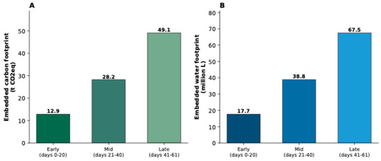
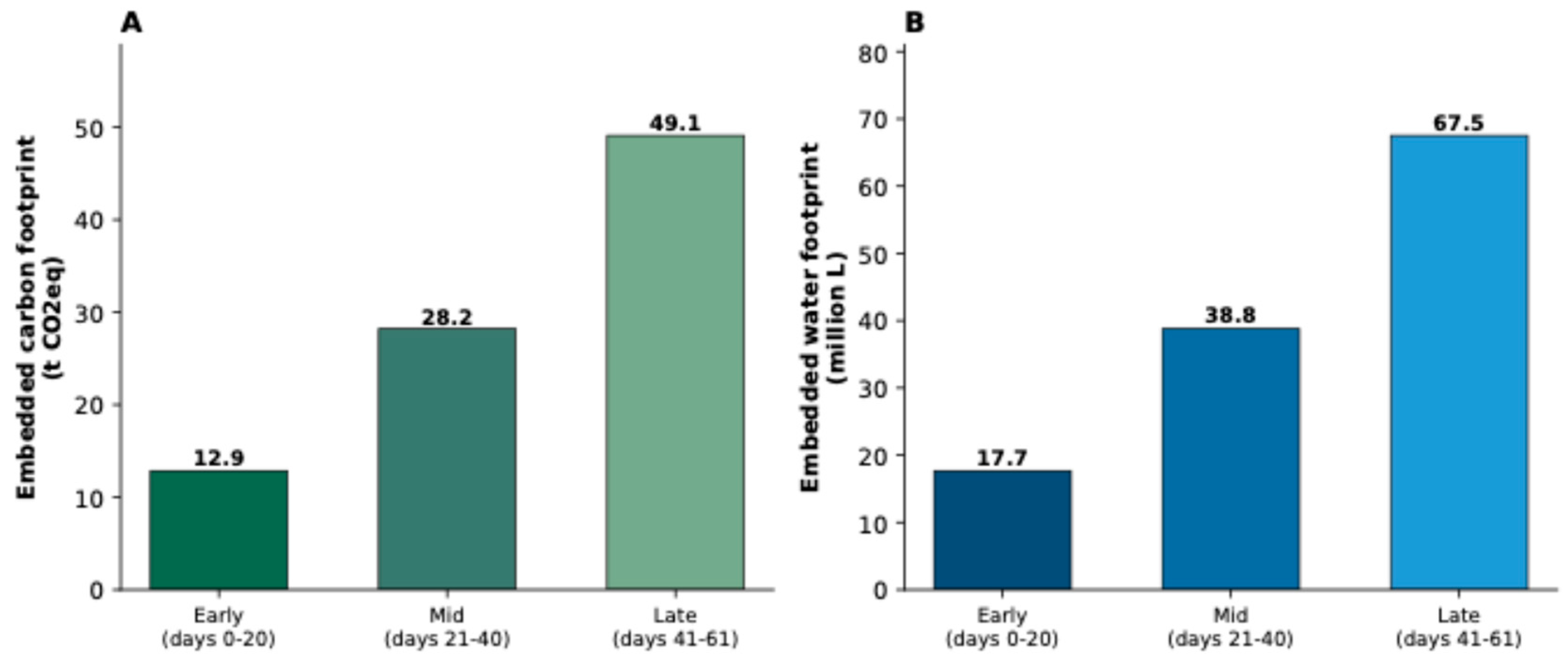
Since the magnitude of waste increases throughout the cycle, its environmental footprint is disproportionately concentrated in the final stages (Figure 5). The potential for mitigation is substantial. In this regard, if waste in the final phase (46.5%) could be reduced to the level of the initial phase (35.6%)—a gap of 10.9 percentage points—approximately 146 metric tons of tomatoes would be recovered, avoiding approximately 21 t CO₂eq (90% CI [6, 40]) and 18 million liters of water (90% CI [11, 27]) in the final stage of the cycle alone. This positions the phased implementation of interventions as a concrete way to contribute to SDG Target 12.3.

Figure 5. Environmental footprint embedded in waste by seasonal phase. Panel (A) shows the carbon footprint (t CO₂eq), and panel (B) shows the water footprint (millions of liters) embedded in the discarded tomatoes in each phase, estimated using central life cycle factors for open-field cultivation (0.080 kg CO₂eq/kg and 110 L/kg). The impact is concentrated in the middle and final phases. These per-phase bars use the modal coefficient for legibility; the Monte Carlo mean reported in the text (Section 3.5) propagates the full coefficient distribution and is correspondingly higher.

4. Discussion

The dissociation between the magnitude and composition of waste throughout the production cycle is the most significant finding of this study. While, on the one hand, the quantity discarded increases markedly and predictably, on the other hand, the structure of the causes generating it remains stable. This distinction, realized through the application of compositional methods, has concrete practical implications. First, it suggests that the increase in waste toward the end of the season is not due to the emergence of new quality problems, but rather to a uniform intensification of the same waste factors present from the outset. The only exception—superficial discoloration, the only category that gains significant relative weight—has a clear physiological basis. In northwestern Mexico, ambient temperatures in late April and May regularly exceed 30 °C, and in this regard, it is noted that, above this temperature threshold, lycopene biosynthesis is strongly inhibited, resulting in irregular coloring, yellow shoulders, and a blotchy ripening appearance that disqualifies the fruit from export categories [7]. Lycopene accumulation operates within a comparatively narrow thermal window, with optimal synthesis between roughly 16 and 26 °C, and its suppression above 30 °C proceeds through reduced phytoene synthase activity together with accelerated thermal degradation of the pigment already formed. Older plants in the final weeks of the growing season also exhibit lower canopy density and greater leaf senescence, which increases the fruit’s exposure to direct solar radiation and thermal load, intensifying the discoloration response. The selective increase in this discolored (clown-faced) category is therefore consistent with the thermal and light stress expected at the end of a growing cycle, especially in arid regions, and links the statistical signal to a specific agronomic mechanism. None of the components of this mechanism—canopy density, fruit surface temperature, radiation load—falls within the packing records, and on the corrected scale, the discoloration trend is exploratory. Therefore, the literature has measured the signal against the established plant physiology, and concurrent field measurements would settle it.

This study also illustrates a methodological risk commonly observed in production data: the confounding of the clustering unit and time. The apparent effect of the production field on waste disappeared when controlling for the time at which each field began operations, revealing it to be a mechanism of processing scheduling rather than an agronomic characteristic of the fields. Whether these fields also differ agronomically is a separate question that cannot be answered by this design: no window exists in which all six fields were jointly observed. This finding serves as a cautionary note for studies that attribute performance differences to units (fields, lines, shifts) without verifying their independence from temporal covariates.

The compositional treatment was decisive. An analysis that considered only crude proportions would have produced spurious correlations induced by the summation constraint, potentially leading to erroneous conclusions about which types of waste predict the total level. The use of log-ratio coordinates—still uncommon in the postharvest literature—separated the true signal from the structural mechanism and constitutes a methodological contribution that can be applied to other loss classification systems. Correcting for multiple comparisons follows the same logic. With seven simultaneous comparisons performed on a single dataset, an apparently significant result arises by chance, with probability near thirty percent.

From a predictive perspective, the performance of Gradient Boosting (R² ≈ 0.90) confirms that daily waste is highly systematic and can be predicted based on simple operational variables. The dominance of the cycle day as a predictor suggests that forecasting is able to help packing houses to anticipate waste levels and dynamically adjust their selection standards, labor planning, and commercial commitments as the season progresses. The validation contrast in Section 3.4 marks how far that prospect currently reaches. Within-cycle reconstruction is well-supported, while an operational forecasting system would need to be fitted on complete cycles and tested on a held-out one.

For quality management, the practical implication follows from the compositional result. Because no single cause gains ground disproportionately as waste increases, improvement programs cannot be expected to find one dominant defect to attack, and interventions inside the plant—sorting calibration, handling, line speed—need to act across the full set of causes simultaneously. Moreover, their expected yield is bounded by the fact that most of the variation is entered with the incoming fruit rather than arising on the line, which locates the larger share of the opportunity upstream, in harvest timing and transport conditions.

From a sustainability perspective, quantifying the environmental footprint is a factor that significantly adds to the reported findings. Waste ceases to be merely an economic loss and emerges as a considerable environmental liability: tens of metric tons of CO₂eq and more than 100 million liters of water incorporated into product that never reached the market, in a single plant and a single cycle. The fact that this impact is concentrated in the final phases of the cycle is, paradoxically, an opportunity. It allows mitigation efforts to be focused on a limited and predictable time window. The proposed predictive model could, for example, be integrated into early-warning systems that anticipate waste peaks and, in turn, trigger recovery protocols—reclassification for secondary markets, processing, or donation—all before the product is discarded. Such mechanisms are directly linked to SDG Target 12.3 and to SDG 2 by recovering food fit for consumption. None of this has been evaluated here beyond the arithmetic of avoided tonnage. Donation and reprocessing channels carry food safety requirements for the handling and traceability of already-graded-out fruit, logistics for same- or next-day collection that current operations were not designed around, and costs that were not measured in this study. These are considered open questions for the pilot study described in the Section 5, not as claims established by the present data. This approach is consistent with the increasing evidence that data-driven predictive models are useful tools for reducing food losses throughout the supply chain [19].

Among the limitations, the single-cycle horizon prevents the separation of seasonal trends from possible structural or interannual effects and limits generalizability to other cycles or plants. With the observation of one cycle, the gradient reported here cannot be distinguished from conditions specific to 2024, a season of exceptional drought and record temperatures in the region. Both the level of waste and the steepness of its rise may carry that context. A seasonal trend and an anomalous year are observationally equivalent in a single-cycle design. The absence of field variables (temperature, variety, days to harvest) restricts the model’s ability to establish causality. Field–time confounding, although correctly diagnosed, also prevents the estimation of a net effect of origin. Environmental estimates are first-order approximations based on factors from the literature with broad ranges, not site-specific inventories. Future studies involving multiple cycles and the processing of fields independently of operating time would allow for the validation and extension of these findings.

5. Conclusions

In this study, we characterized the temporal and compositional dynamics of waste in export-quality tomato packaging in northwestern Mexico and quantified its embedded environmental footprint. As a single-plant, single-cycle study, the findings describe this system during one season and should not be generalized without replication. The magnitude of waste grew steadily throughout the cycle (+1.8 percentage points per week, 95% CI [1.59, 2.05], robust to autocorrelation-consistent standard errors; r = 0.75), while no significant change in its composition by discard cause was detected (multivariate test: p = 0.135; block permutation: p = 0.168), though an equivalence test could not confirm stability either. Only discolored fruit increased in relative weight, a tendency that is considered exploratory based on the corrected scale (p = 0.159), which is consistent with the heat-induced inhibition of lycopene synthesis characteristic of the region at the end of the cycle. The production cycle helps determine how much tomato is wasted, not why they are discarded. Apparent differences between fields were confounded with their operating windows, which this design cannot separate, as illustrated most clearly by field M 3-3, the entire record of which falls in the last quintile of the cycle. A Gradient Boosting model was used with only variables available before sorting to predict daily waste, achieving an accuracy of R² = 0.846, with RMSE = 2.16 pp, which is close to the R² = 0.898 obtained when adding same-day grading variables, within the observed cycle; extension to cycles not yet observed requires multi-cycle data, since time-blocked validation showed that neither version outperformed the training mean, with the cycle day being the dominant factor in relative importance, not in variance explained. The discarded product accounted for an estimated footprint of 162 t CO₂eq (90% CI [50, 310]) and 141 million liters of water (90% CI [81, 209]), obtained by propagating the uncertainty of the underlying life cycle coefficients rather than applying a single central value, and concentrated in the final phases. Closing the gap between the end and beginning of the cycle would prevent approximately 21 t CO₂eq and 18 million liters of water.

These findings point to a candidate direction for future pilot work rather than a conclusion this study demonstrates: they identify a window of elevated risk, while the feasibility and cost of acting on it fall outside the scope of the present analysis and remain to be established. Since the discoloration-driven rise in waste is predictable from the cycle’s midpoint, a natural next step would be for packing houses to pilot standing agreements with processors and food banks to absorb the anticipated surplus, subject to the feasibility, food-safety, and cost assessment such a pilot would require. If shown to be viable, this could divert otherwise-discarded fruit into processed or donated food, supporting SDG Target 12.3 and, through recovery, SDG 2. Coupled with the predictive model as an early-warning trigger, such a pilot could in principle enable proactive rather than reactive recovery logistics. Testing this proposal—including its cost-effectiveness relative to current practice—is a specific objective of the follow-up study now under way.

References

- USDA-FAS. Mexico: Tomatoes and Products Annual; Report MX2024-0028; United States Department of Agriculture, Foreign Agricultural Service: Washington, DC, USA, 2024. Available online: https://www.fas.usda.gov/data/gain/2024/06/mexico-tomatoes-and-products-annual (accessed on 5 December 2025).
- USDA-FAS. Mexico: Tomatoes and Products Annual; Report MX2025-0026; United States Department of Agriculture, Foreign Agricultural Service: Washington, DC, USA, 2025. Available online: https://www.fas.usda.gov/search?keyword=Mexico%3A+Tomatoes+and+Products+Annual%3B+Report+MX2025-0026 (accessed on 5 December 2025).
- DATA MÉXICO. Producto: Tomates Frescos o Refrigerados; Gobierno de México Secretaría de Economía: Ciudad de Mexico, Mexico, 2026. Available online: https://www.economia.gob.mx/datamexico/es/profile/product/tomatoes-fresh-or-chilled-2070200?exportsGeoSelector=1&importsGeoSelector=1 (accessed on 26 June 2026).
- CONAGUA. Monitor de Sequía en México: Reporte del Ciclo Agrícola 2024–2025; Comisión Nacional del Agua: Ciudad de Mexico, Mexico, 2025. Available online: https://smn.conagua.gob.mx/es/climatologia/monitor-de-sequia/monitor-de-sequia-en-mexico (accessed on 4 September 2026).
- Pronatura Noroeste. Water Crisis Hits Northwestern Mexico: Aquifer Overexploitation and Irrigation Deficits in Sonora and Sinaloa; Technical Note; Prematura Noroeste: Ensenada, Mexico, 2025; Available online: https://pronatura-noroeste.org/ (accessed on 4 September 2026).
- Arah, I.K.; Amaglo, H.; Kumah, E.K.; Ofori, H. Preharvest and postharvest factors affecting the quality and shelf life of harvested tomatoes: A mini review. Int. J. Agron. 2015, 2015, 478041. [Google Scholar] [CrossRef] [Scilit]
- Al-Dairi, M.; Pathare, P.B.; Al-Yahyai, R.; Opara, U.L. Mechanical damage of fresh produce in postharvest transportation: Current status and future prospects. Trends Food Sci. Technol. 2022, 124, 195–207. [Google Scholar] [CrossRef] [Scilit]
- FAO. Postharvest Management of Tomato for Quality and Safety Assurance; Food and Agriculture Organization of the United Nations: Rome, Italy, 2018; Available online: https://openknowledge.fao.org/server/api/core/bitstreams/bf0662e4-1469-4336-b93a-1d9aaf84c1bf/content (accessed on 9 March 2024).
- Kefas, B.E.; Aliyu, B.; Tashiwa, Y.I. Postharvest losses, causes and mitigation in tomato transportation: A systematic review. J. Hortic. Postharvest Res. 2024, 7, 223–236. [Google Scholar] [CrossRef]
- UNEP. Food Waste Index Report 2021; United Nations Environment Programme: Nairobi, Kenya, 2021; Available online: https://wedocs.unep.org/handle/20.500.11822/35280 (accessed on 9 March 2024).
- United Nations. Transforming Our World: The 2030 Agenda for Sustainable Development; A/RES/70/1; United Nations General Assembly: New York, NY, USA, 2015; Available online: https://docs.un.org/en/A/RES/70/1 (accessed on 17 March 2024).
- Kissinger, M. Tomatoes from the desert: Environmental footprints and sustainability potential in a changing world. Front. Sustain. Food Syst. 2022, 6, 994920. [Google Scholar] [CrossRef] [Scilit]
- Page, G.; Ridoutt, B.; Bellotti, B. Carbon and water footprint tradeoffs in fresh tomato production. J. Clean. Prod. 2012, 32, 219–226. [Google Scholar] [CrossRef] [Scilit]
- Al Shoffe, Y.; Johnson, L.K. Opportunities for prediction models to reduce food loss and waste in the postharvest chain of horticultural crops. Sustainability 2024, 16, 7803. [Google Scholar] [CrossRef] [Scilit]
- Aitchison, J. The statistical analysis of compositional data. J. R. Stat. Soc. Ser. B 1982, 44, 139–177. [Google Scholar] [CrossRef] [Scilit]
- Greenacre, M. Compositional data analysis. Annu. Rev. Stat. Appl. 2021, 8, 271–299. [Google Scholar] [CrossRef] [Scilit]
- Fawole, O.A. Machine learning application in horticulture and prospects for predicting fresh produce losses and waste: A review. Plants 2024, 13, 1200. [Google Scholar] [CrossRef] [Scilit] [PubMed]
- Lakens, D. Equivalence Tests: A Practical Primer for t Tests, Correlations, and Meta-Analyses. Soc. Psychol. Personal. Sci. 2017, 8, 355–362. [Google Scholar] [CrossRef] [Scilit] [PubMed]
- Lakens, D.; Scheel, A.M.; Isager, P.M. Equivalence Testing for Psychological Research: A Tutorial. Adv. Methods Pract. Psychol. Sci. 2018, 1, 259–269. [Google Scholar] [CrossRef] [Scilit]
- Zhu, Z.; Miller, S.A. Greenhouse gas emissions of tomato production and supply: A systematic review. Resour. Conserv. Recycl. 2025, 218, 108236. [Google Scholar] [CrossRef] [Scilit]
- Mekonnen, M.M.; Hoekstra, A.Y. The green, blue and grey water footprint of crops and derived crop products. Hydrol. Earth Syst. Sci. 2011, 15, 1577–1600. [Google Scholar] [CrossRef] [Scilit]
Disclaimer/Publisher’s Note: The statements, opinions and data contained in all publications are solely those of the individual author(s) and contributor(s) and not of MDPI and/or the editor(s). MDPI and/or the editor(s) disclaim responsibility for any injury to people or property resulting from any ideas, methods, instructions or products referred to in the content. |
© 2026 by the authors. Licensee MDPI, Basel, Switzerland. This article is an open access article distributed under the terms and conditions of the Creative Commons Attribution (CC BY) license.