


Abstract
Achieving the Sustainable Development Goals (SDGs) requires a transition from conventional fossil-fuel-powered vehicles to alternative energy sources, such as electricity. However, reliably predicting energy consumption under highly variable real-world driving conditions and across different temporal horizons remains a critical challenge regarding the widespread adoption of Electric Vehicles (EVs), directly impacting the precision of range estimation, route planning, and charging strategies. To address this, a novel approach is proposed, combining advanced machine learning models—such as XGBoost, Random Forest, and regression-based techniques—with innovative dataset manipulation using statistical methods. The methodology integrates feature engineering to incorporate vehicle-specific metrics, including driving patterns and environmental conditions, ensuring that models dynamically adapt to real-world scenarios. The proposed framework demonstrates high accuracy and robustness in predicting energy consumption, providing valuable insights for sustainable transportation and efficient energy management toward SDG achievement.
1. Introduction
The global shift from traditional fossil fuels to renewable energy sources represents a significant step toward achieving the Sustainable Development Goals (SDGs) [1]. In the context of sustainable transportation, the transition to electric vehicles (EVs) is a key component, directly supporting SDG 11 (i.e., Sustainable Cities and Communities) and SDG 13 (i.e., Climate Action) by offering a zero-emission alternative to conventional internal combustion engine vehicles [2]. Furthermore, accurate EV energy consumption forecasting contributes to SDG 7 (i.e., Affordable and Clean Energy) by enabling optimized battery usage, minimized energy waste, and grid-friendly smart charging scheduling. However, despite their growing adoption, several challenges still hinder their widespread use, including limited driving range, long charging times, battery cost, and battery weight [3].
Energy consumption plays a crucial role in EV operation, as it directly affects vehicle efficiency, route planning, and charging scheduling [4]. This is particularly important because EV energy consumption is highly dynamic and is influenced by several factors, including driving patterns, traffic conditions, weather, and vehicle-specific characteristics [5]. Therefore, one of the most prominent challenges is the accurate prediction of energy consumption under varying driving conditions [6]. Accurate energy consumption forecasts can help drivers better manage vehicle performance, contributing to more efficient driving and energy usage [7]. More broadly, they can support the optimized use of EVs, particularly with respect to battery management. In contrast, poor energy consumption predictions may lead to inefficient charging infrastructure planning, increased range anxiety, and suboptimal energy management strategies [8].
Several machine learning models have been employed to improve prediction accuracy. However, the main problem this research addresses is the inability of existing forecasting frameworks to dynamically and reliably predict EV energy consumption across multiple temporal resolutions under highly variable real-world driving conditions. Existing approaches often fail to adequately capture the temporal dependencies and variability inherent in real-world driving scenarios [9]. For instance, many models rely on static datasets [10], which do not fully account for fluctuating energy demands caused by stop-and-go traffic, elevation changes, or extreme weather conditions. This limitation reduces the reliability of predictions and may undermine user confidence in EVs, thereby slowing their adoption.
Energy consumption forecasting, particularly for longer-term prediction horizons, is also essential for effective infrastructure planning [11]. Accurate forecasting can support the optimal placement of charging stations and the efficient management of energy distribution. Moreover, as the EV market continues to expand, existing infrastructure is expected to face increasing demand, making the development of reliable energy consumption forecasting models increasingly important [12]. Addressing these challenges is therefore fundamental to ensuring the long-term viability of electric vehicles and facilitating a seamless transition toward sustainable transportation.
In this article, a forecasting framework for EV energy consumption is proposed, leveraging machine learning models and data preprocessing techniques that include statistical feature characterization. More specifically, the proposed approach uses a publicly available dataset to address the energy consumption forecasting problem as follows: (i) incorporating feature engineering to capture vehicle-specific variables and environmental conditions, ensuring adaptability to diverse real-world scenarios; (ii) performing statistical analysis of the extracted features; and (iii) employing machine learning algorithms, including XGBoost, Random Forest, Dynamic Linear Regression, and ARIMA. The objective of this study is to provide accurate energy consumption predictions that support sustainable transportation, efficient battery usage, and improved energy management.
The remainder of this paper is structured as follows: Section 2 provides a review of related work, highlighting current advancements and limitations in EV energy consumption forecasting. Section 3 describes the eVED dataset used in this study. Section 4 presents the proposed methodology, including preprocessing and temporal aggregation, feature engineering and lag construction, lag-based input configurations, forecasting models, model training and hyperparameter optimization, and evaluation metrics. Section 5 presents the experimental results and discusses their implications, while Section 6 provides a comprehensive discussion on the generalizability, temporal forecasting horizons, and scalability challenges of the proposed framework for large-scale fleets. Finally, Section 7 concludes the paper and outlines potential future research directions.
2. Related Work
In recent years, the rise of EVs has driven extensive research into the optimization of their energy consumption. This has led to the development of machine learning models for predicting energy usage, as well as applications designed to help users manage their vehicles more efficiently. The following paragraphs present representative studies focusing on EV energy consumption forecasting.
Huang et al. [13] introduced a novel approach to understanding the factors influencing EV energy consumption. Their study addresses a key limitation of previous research, which primarily examined statistical correlations without exploring causal relationships. By applying double/debiased machine learning combined with bootstrap-of-little-bags inference, the authors inferred how different factors affect energy consumption. An important finding of their work is that driving speeds around 50 km/h can lead to improved energy consumption rates.
Petkevicius et al. [14] addressed the growing challenge of EV energy consumption prediction, particularly in long-distance route planning, by using eight deep learning models. The authors proposed a two-tier architecture for forecasting both energy consumption and travel time. The first tier consists of a routing and travel-time prediction subsystem that generates a suggested route and predicts speed variations. The second tier predicts energy consumption based on speed profiles, weather conditions, and road slope. According to their experiments, realistic time-specific speed profiles provided the best results.
Hua et al. [15] proposed a method for accurately estimating EV energy consumption, emphasizing its importance for optimizing charging station deployment, promoting eco-friendly driving practices, and extending EV range. Their approach comprises three key components: segmentation-assisted trajectory granularity, knowledge transfer from internal combustion engine and hybrid electric vehicles to EVs, and time-series estimation using a bidirectional recurrent neural network (RNN). Their RNN-based methodology achieved the best performance compared with several conventional methods, including tree-based, regression-based, and support vector machine approaches.
Athanasakis et al. [16] introduced a methodology for forecasting the State of Charge (SoC) in EVs. Their approach integrates lightweight regression-based models with feature engineering to enhance SoC prediction accuracy. To validate the effectiveness of their methodology, experiments were conducted on both a private dataset of automated EVs and a public EV dataset. The results demonstrated the efficiency of their lightweight approach and its superiority over more computationally intensive methods, such as deep learning models and gradient boosting algorithms.
Chen et al. [17] addressed the challenges of energy consumption estimation in EVs, particularly in scenarios where certain features are unavailable. To account for uncertainties introduced by transient factors, the authors implemented an XGBoost prediction model, which outperformed other approaches in point-value energy consumption estimation. An important outcome of their explanatory analysis is that the relevance of specific features to energy consumption can vary depending on road type.
Tang et al. [18] presented a predictive energy management approach that optimizes energy consumption for plug-in hybrid electric vehicles (PHEVs) using travel route data. Their methodology incorporates battery temperature as an optimization factor in the energy cost function and employs an extreme learning machine as a short-term speed predictor. By training the speed predictor on historical real-world speed data and integrating travel route information, the study achieved higher forecasting accuracy than traditional driving cycles.
Polymeni et al. [19] developed a machine learning-based approach for energy consumption forecasting in fuel cell electric vehicles (FCEVs). Their methodology incorporated techniques from three distinct machine learning families: statistical-based models, ensemble methods, and deep learning. Using an artificial dataset of hydrogen vehicles generated through the Future Automotive Systems Technology Simulator [20], together with real-world booking records from an on-demand public transportation service in the Geneva Canton region, they achieved high forecasting accuracy, with errors remaining below 10%.
Similarly, in the broader energy forecasting domain, Baratsas et al. [21] developed a comprehensive hybrid framework incorporating 40 different statistical and machine learning techniques, including ARIMA, exponential smoothing, and deep neural networks, to forecast prices across numerous energy products. Their findings underscore that while advanced machine learning models often deliver superior results over traditional statistical baselines, systematic hyperparameter optimization via grid search remains essential to ensuring maximum predictive performance.
Beyond standalone vehicle performance, accurate energy consumption and driving condition forecasting have significant implications for both vehicle-side energy management and grid-side infrastructure. On the vehicle side, accurate long-term predictive information supports hierarchical controllers in managing complex trade-offs, such as optimizing power-split strategies in hybrid vehicles to mitigate power source aging and degradation of batteries or fuel cells [22], while on the grid side, forecasting helps address the control stability challenges of EV charging networks integrated into low-voltage DC distribution systems. These vehicle-side optimal control strategies frequently depend on pre-specified performance indices. To address scenarios where target performance weights are unknown, Zhou and Li [23] proposed an inverse optimal control (IOC) framework for high-order nonlinear fully actuated systems (FASs) to learn unknown reward weights from expert trajectories. Their work demonstrates how learning-based optimization can stabilize complex systems and enhance control performance, providing a useful analog for optimizing the parameters of highly dynamic EV energy management systems. Because sudden charging load variations can trigger resonance and stability issues in DC microgrids, advanced control frameworks on the grid side [24] rely on stable demand forecasting to maintain voltage regulation and power quality. Integrating robust energy consumption forecasting can therefore close the gap between vehicle-side power demand and grid-side supply stability.
Overall, existing studies have examined EV energy consumption from different perspectives. Some works focus on understanding and explaining energy usage based on external factors such as speed, environmental conditions, and terrain [13,17]. Others employ deep learning-based forecasting methods to predict energy consumption in EVs [14,15], while lightweight regression-based frameworks have also been proposed for related prediction tasks, such as SoC estimation [16]. In addition, several studies apply machine learning techniques to forecast energy consumption across different types of electric vehicles, including PHEVs and FCEVs [18,19].
This work differs from existing studies by introducing a comprehensive machine learning-based framework for EV energy consumption forecasting across multiple temporal aggregation intervals, namely 1 min, 5 min, and 10 min intervals. The proposed methodology systematically evaluates different model families, including Random Forest, XGBoost, Dynamic Linear Regression, and ARIMA, while also investigating three lag-based input configurations: historical energy consumption values, lagged external vehicle-related features, and their combination. This design enables the predictive contribution of both endogenous and exogenous information to be assessed in a consistent manner. Unlike many previous studies that focus on a single feature representation or forecasting horizon, this work examines the impact of key operational and contextual factors, including vehicle speed, acceleration, elevation, air-conditioning power, and heater power, on EV energy consumption. Furthermore, the use of statistical feature characterization within aggregated time intervals provides additional insight into the distribution of and variability in the contributing factors. Overall, the main contribution of this work lies in the systematic comparison of model families, temporal resolutions, and lag-based input structures within a unified EV energy consumption forecasting framework.
3. Dataset Description
Zhang et al. [25] introduced the extended Vehicle Energy Dataset (eVED), an enhancement of the well-established Vehicle Energy Dataset [26], designed to provide more accurate vehicle trip data for large-scale energy consumption analysis. The eVED dataset ensures data sufficiency for machine learning applications by incorporating precise GPS coordinates and enriched features. It includes a comprehensive set of variables that capture both internal vehicle dynamics and external environmental factors, essential for understanding vehicle behavior and traffic patterns. The dataset contains three electric vehicles (vehicle 10, vehicle 455, and vehicle 541) with diverse operational characteristics, all of which were utilized in this study. Structurally, eVED is formatted as a time series, representing vehicle routes and their corresponding data over time.
Compared to other datasets commonly used in energy consumption research, such as simulated datasets [19] or aggregated trip-level records [27,28], eVED offers a higher temporal resolution by capturing real-world driving conditions at minute-level intervals. This fine granularity enables detailed temporal analysis and improves machine learning models’ ability to capture short-term fluctuations in energy usage. Key features influencing energy consumption predictions include vehicle speed, air-conditioning power, heater power, and smoothed elevation data, as presented in Table 1. These variables provide insights into both vehicle performance and the external factors affecting energy consumption. As a result, the eVED dataset serves as a valuable and diverse resource for robust energy consumption modeling across various driving conditions and vehicle types.
Table 1.
eVED Dataset Raw Data Variables.
4. Methodology
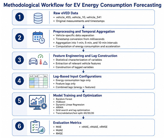
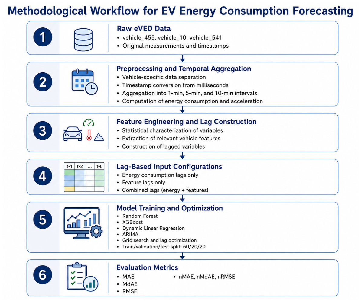
The proposed methodology follows a structured forecasting pipeline for predicting electric vehicle (EV) energy consumption using the eVED dataset. As shown in Figure 1, the workflow starts from the raw eVED data, which are described in the dataset section, and proceeds through five methodological stages: preprocessing and temporal aggregation, feature engineering and lag construction, lag-based input configuration, forecasting model development and optimization, and performance evaluation. The workflow transforms the raw eVED data into vehicle-specific lag-based input spaces, which are then used for model training, optimization, and evaluation.
Figure 1.
Methodological workflow for energy forecasting.
4.1. Preprocessing and Temporal Aggregation
To ensure the compatibility of the eVED dataset with the selected forecasting algorithms, a series of preprocessing and data preparation steps was performed. This stage constitutes a key part of the proposed methodology, as it transforms the raw vehicle measurements into structured time-series datasets suitable for energy consumption forecasting.
As previously described, the dataset includes three EVs, namely vehicle_455, vehicle_10, and vehicle_541. Initially, the data were separated according to vehicle ID in order to construct vehicle-specific datasets. This step was necessary because each vehicle may exhibit distinct driving patterns, operating conditions, and energy consumption characteristics.
The original timestamps, which were recorded in milliseconds, were then converted into consistent time-based representations. The data were aggregated into one-minute, five-minute, and ten-minute intervals, resulting in three temporal resolutions for each vehicle. This aggregation enabled the calculation of energy consumption and acceleration over fixed time windows, while also supporting the investigation of how different temporal granularities affect forecasting performance.
Following the temporal aggregation process, a statistical characterization of the resulting variables was performed. Inspired by the relevant literature [29], descriptive statistics such as mean, median, minimum, maximum, and standard deviation were computed for each feature within each aggregated time window. Rather than relying on simple downsampling, which discards valuable high-frequency information, this statistical characterization preserves intra-interval dynamics and variability, providing the models with rich, multi-dimensional feature representations that capture the volatility and distribution of driving behaviors and auxiliary system demands within each interval, thereby significantly enhancing forecasting robustness and accuracy. This analysis provided a clearer understanding of the structure of, variability in, and distribution of the processed data. The initial variables of the dataset and the variables obtained after preprocessing are presented in Table 1 and Table 2, respectively.
Table 2.
eVED Dataset Processed Data Variables.
Overall, the preprocessing and temporal aggregation stage ensured consistency across the vehicle-specific time series and produced the structured datasets used in the subsequent forecasting pipeline.
4.2. Feature Engineering and Lag Construction
After preprocessing, feature engineering was performed to extract the variables most relevant to EV energy consumption forecasting. The selected features included vehicle-related and operational variables such as vehicle speed, acceleration, air-conditioning power, heater power, and smoothed elevation. The complete list of all processed variables utilized in the forecasting models is offered in Table 2. These variables were selected because they capture important aspects of vehicle dynamics, auxiliary system usage, and driving conditions that may influence energy demand.
In addition to the direct use of these explanatory variables, lagged variables were constructed to capture temporal dependencies in the data. Lag construction is essential for time-series forecasting, as future energy consumption may depend not only on current vehicle conditions but also on previous consumption patterns and past operating states. Therefore, lagged versions of both the target variable and the external vehicle-related features were created.
The number of lagged observations was not fixed a priori. Instead, different lag structures were examined during model optimization in order to identify the most suitable temporal dependencies for each vehicle, temporal aggregation interval, and forecasting model.
4.3. Lag-Based Input Configurations
To investigate the predictive contribution of different sources of temporal information, three lag-based input configurations were defined. These configurations were designed to assess whether future energy consumption is better explained by its own historical values, by external vehicle-related features, or by a combination of both:
- Energy Consumption Lags Only: This configuration uses only historical values of energy consumption to predict future consumption. It is designed to capture autocorrelation patterns in the target variable [30].
- Feature Lags Only: This configuration uses only lagged values of external explanatory features, such as vehicle speed, acceleration, air-conditioning usage, heater power, and elevation. Historical values of energy consumption are excluded. This setup evaluates the extent to which vehicle operating conditions can explain future energy demand [31].
- Combined Lags: This configuration incorporates both historical energy consumption values and lagged external vehicle-related features. It provides a more comprehensive input representation by combining past consumption behavior with vehicle operating conditions, following the rationale of approaches that exploit both target-variable history and external contextual features for temporal prediction tasks [32].
These configurations were applied across the different temporal aggregation intervals, namely one-minute, five-minute, and ten-minute datasets. This allowed the analysis to examine not only the effect of the input structure, but also the influence of temporal resolution on forecasting performance.
For Random Forest and XGBoost, all three input configurations were implemented: energy consumption lags only, feature lags only, and combined lags. For the regression-based models, Dynamic Linear Regression was used to model configurations involving exogenous variables, including the feature-lag and combined-lag settings. ARIMA was used for the configuration based exclusively on historical energy consumption values, without incorporating exogenous inputs.
4.4. Forecasting Models
Considering their strong performance in a wide range of prediction tasks [7,19,33,34,35,36], models from different algorithmic families were selected to evaluate the robustness and generalizability of the proposed feature engineering approach under varying mathematical structures. Specifically, the proposed methodology evaluates Random Forest [37], XGBoost [38], Dynamic Linear Regression [39], and ARIMA, representing distinct, well-established approaches to time-series forecasting, with non-parametric tree ensembles being chosen for their capacity to capture highly non-linear feature interactions and resist multicollinearity, while parametric regression models serve as interpretable baselines to isolate linear relationships, and univariate statistical models establish a benchmark based purely on target auto-correlation. The use of multiple well-established machine learning and time-series forecasting models is consistent with common practice in the literature [19], particularly when the objective is to evaluate a new forecasting framework rather than introduce a new learning algorithm. Consequently, rather than employing deep learning architectures, such as recurrent neural networks (RNNs) that are prone to overfitting on the moderate sample sizes of this study (i.e., 1 min, 5 min, and 10 min temporal aggregations) [40], our work focused on more classical regression and statistical families. This design choice supports a more robust assessment of the proposed framework and enables its performance to be examined across different model families.
In this context, random Forest was selected because of its robustness, ability to model nonlinear relationships, and reduced tendency to overfit through ensemble learning. Wang et al. [41] and Pang et al. [42] highlighted Random Forest as a promising method for energy prediction, demonstrating its stability and strong fitting capability. In this study, the Random Forest model was trained using the lag-based input configurations described above and was evaluated across the three temporal aggregation intervals. Indeed, it is common practice in the literature [19] to employ multiple well-established machine learning algorithms when proposing a new framework—as is the case in this work—rather than introducing a novel ML methodology. This approach supports the generalization and robustness of the proposed framework.
XGBoost was also employed due to its efficiency, scalability, and strong predictive performance on structured datasets. As a gradient boosting algorithm, XGBoost iteratively improves prediction accuracy by learning from previous errors, while its built-in regularization mechanisms help reduce overfitting. These properties make it suitable for EV energy forecasting, where diverse driving conditions and nonlinear relationships may be present. The model was trained using the same temporal resolutions and lag-based input configurations as Random Forest.
Dynamic Linear Regression was used as an interpretable regression-based forecasting approach. This model incorporates lagged values of the target variable and/or exogenous variables, depending on the input configuration. By explicitly modeling lagged dependencies, Dynamic Linear Regression enables the examination of how previous energy consumption and external vehicle-related factors affect future energy usage. Its simplicity and interpretability also make it useful as a baseline for comparing more complex machine learning models.
Finally, an AutoRegressive Integrated Moving Average (ARIMA) model was implemented as a purely time-series baseline. ARIMA models temporal dependencies using autoregressive and moving-average components and can also address non-stationary behavior through differencing [43]. As discussed by Moslemi et al. [44], ARIMA is suitable for energy consumption forecasting when the objective is to model historical patterns in the target variable without relying on exogenous features.
4.5. Model Training and Hyperparameter Optimization
To optimize forecasting performance, grid search was employed to identify suitable hyperparameter configurations for each model. Grid search [45] is an exhaustive search technique that evaluates different combinations of hyperparameters and selects the configuration that provides the best validation performance.
The dataset was divided into training, validation, and testing subsets using a 60:20:20 split, in line with the literature [34,35]. To avoid data leakage, a strict chronological indexing split was enforced across all configurations, and shuffling was completely disabled, ensuring that the temporal dependencies of the driving cycles were preserved and that the models were validated and tested strictly on future, unseen intervals. The training set was used to fit the models, the validation set was used for hyperparameter tuning and lag selection, and the test set was used for the final evaluation of forecasting performance. The full hyperparameter tuning grids, parameter search steps, and chronological splitting parameters are detailed in Table 3.
Table 3.
General rules, hyperparameter search grids, and optimal lag configurations.
For the Random Forest model, a search was evaluated over multiple parameter ranges, as specified in Table 3. Ultimately, 300 decision trees were used to improve robustness and reduce variance. The maximum tree depth was set to 20, providing a balance between model complexity and generalization. The minimum number of samples required to split an internal node was set to 2, allowing the trees to grow sufficiently while preserving predictive accuracy. A fixed random seed was used to ensure reproducibility.
For the XGBoost model, several hyperparameter combinations were evaluated, using the grid search boundaries and step sizes outlined in Table 3. The best-performing configuration used a maximum tree depth of 3, a learning rate of 0.2, and 300 boosting rounds. The squared error objective function was used, as it is appropriate for regression tasks. Early stopping was incorporated to prevent overfitting, and a fixed random seed was used to ensure reproducibility.
For the Dynamic Linear Regression models, lag selection was performed for both the target variable and the exogenous variables, including vehicle speed, acceleration, elevation, air-conditioning power, and heater power. A grid search evaluating lags from 1 to 10 was performed across all temporal aggregation resolutions (1 min, 5 min, and 10 min intervals), and the optimal lag orders identified for each specific vehicle are documented in Table 3. The most effective configuration included up to four lagged observations, allowing the model to capture short-term temporal dependencies, as well as longer-term trends in energy consumption.
A similar tuning procedure was applied to the ARIMA model. Following a grid search over the AR, differencing, and MA ranges defined in Table 3, an ARIMA (3, 0, 1) configuration was found to be effective across the examined vehicles and datasets. The autoregressive component of order 3 uses three lagged observations of energy consumption, the differencing order of 0 indicates that no differencing was required, and the moving-average component of order 1 uses one lagged forecast error to correct future predictions.
Beyond model-specific hyperparameter tuning, lag optimization was performed for each algorithm and sub-dataset. Since each vehicle was represented at three temporal resolutions, namely one-minute, five-minute, and ten-minute intervals, the optimal number of lagged observations could vary across vehicles, aggregation intervals, and model types. This process ensured that each model was adapted to the temporal characteristics of the corresponding dataset.
4.6. Evaluation Metrics
Model performance was evaluated using Mean Absolute Error (MAE), Median Absolute Error (MdAE), and Root Mean Squared Error (RMSE), along with their normalized versions. These metrics were selected because they are widely used in forecasting and energy prediction studies [19,46,47]. They provide complementary perspectives on model performance by measuring average error magnitude, robustness to outliers, and sensitivity to larger prediction errors.
The Mean Absolute Error is defined as
where denotes the error between the actual and predicted energy consumption values, and n is the number of observations.
The Median Absolute Error is defined as
This metric represents the median absolute prediction error and is therefore more robust to outliers than MAE.
The Root Mean Squared Error is defined as
RMSE penalizes larger errors more strongly because of the squared error term, making it particularly useful when large deviations from the actual values are undesirable.
4.7. Use of Generative Artificial Intelligence
OpenAI ChatGPT (model/version: GPT-5.5 Thinking; OpenAI, San Francisco, CA, USA) was used to assist with the visual organization and refinement of Figure 1, which graphically summarizes the proposed methodological workflow. The tool was not used for study design, data collection, data preprocessing, software implementation, model training, hyperparameter optimization, statistical analysis, definition of evaluation metrics, generation of numerical results, or interpretation of the experimental findings.
5. Experimental Results
This section presents the experimental results obtained from the evaluation of the proposed EV energy consumption forecasting framework. The experiments were conducted using the selected vehicles from the eVED dataset and the three temporal aggregation intervals defined in the methodology: 1 min, 5 min, and 10 min intervals. Table 4 presents the evaluation results for the examined model-input configurations, vehicles, and temporal aggregation intervals. For Vehicle 541, only the 1-min interval was considered due to the limited number of available observations; therefore, no models were trained or evaluated at the 5-min and 10-min intervals.
Table 4.
Performance of the evaluated model-input configurations across vehicles and temporal aggregation intervals.
For clarity, each evaluated forecasting configuration is denoted using the model acronym followed by the corresponding input configuration. Specifically, ECL denotes the use of energy consumption lags only, FL denotes the use of lagged external vehicle-related features only, and CL denotes the combined use of energy consumption lags and feature lags. Accordingly, the evaluated configurations are RF-ECL, RF-FL, RF-CL, XGB-ECL, XGB-FL, XGB-CL, DLR-FL, DLR-CL, and ARIMA-ECL. Dynamic Linear Regression is evaluated only with feature-based and combined lag configurations, while ARIMA-ECL is used as a univariate time-series baseline based exclusively on historical energy consumption values.
At the 1 min interval, XGBoost-based configurations achieved the lowest errors for Vehicles 455 and 10. For Vehicle 455, XGB-CL achieved an MAE of 0.04152, an RMSE of 0.05786, and an MdAE of 0.03044, demonstrating its ability to capture short-term variations in energy consumption when both historical consumption and external feature lags are used. Similarly, for Vehicle 10, XGB-CL achieved the lowest errors across all three evaluation metrics, with an RMSE of 0.07156. However, the results were vehicle-dependent, as RF-ECL achieved the lowest MAE, RMSE, and MdAE for Vehicle 541. This indicates that although XGBoost performed strongly at short temporal resolutions, the optimal configuration may vary depending on vehicle-specific driving and consumption patterns.
Random Forest also provided robust results at the 1 min interval. In particular, RF-CL and RF-FL achieved competitive performance for Vehicles 455 and 10, while RF-ECL performed particularly well for Vehicle 541. Dynamic Linear Regression produced reasonable results, especially for Vehicles 455 and 10, but generally did not outperform the best tree-based configurations. ARIMA-ECL showed higher errors for Vehicles 455 and 10, reflecting the limitations of relying exclusively on historical energy consumption values when short-term vehicle dynamics and external factors influence energy demand.
At the 5 min interval, data aggregation resulted in larger absolute prediction errors across most configurations. For Vehicle 455, XGB-FL achieved the lowest MAE, RMSE, and MdAE values, indicating that lagged external vehicle-related features alone were highly informative at this temporal resolution. XGB-CL also remained competitive, with an RMSE of 0.23006. For Vehicle 10, the results were more metric-dependent. RF-FL achieved the lowest MAE, RF-ECL achieved the lowest MdAE, while both DLR-CL and DLR-FL achieved the lowest RMSE of 0.21523. This behavior, i.e., where the two DLR configurations produce identical predictions and evaluation metrics across certain vehicle–interval combinations, is attributed to the linear structure of the DLR model and the reduced sample sizes of these aggregated datasets. When the lagged external vehicle-related features already fully capture the relevant temporal variation, the additional target-variable lags in DLR-CL do not provide extra explanatory power, leading both configurations to converge to equivalent predictions [39]. As a result, this suggests that, under certain aggregation intervals, simpler regression-based models can effectively capture the relationship between lagged explanatory variables and energy consumption, while Random Forest remains competitive depending on the selected evaluation metric.
Random Forest maintained stable performance at the 5 min interval, although it generally trailed the best-performing XGBoost configuration for Vehicle 455 in terms of all three metrics. ARIMA-ECL produced higher errors than most feature-based and combined-lag configurations, particularly for Vehicle 10. This suggests that the inclusion of exogenous vehicle-related variables can improve forecasting accuracy compared with models that rely only on past energy consumption values.
At the 10 min interval, the results became more dependent on the specific vehicle and input configuration. For Vehicle 455, RF-ECL achieved the lowest MAE and RMSE values, while XGB-CL achieved the lowest MdAE. This indicates that, for this vehicle and temporal resolution, historical energy consumption values provided strong predictive information, although the combined-lag XGBoost configuration remained competitive. In contrast, for Vehicle 10, XGB-CL achieved the best RMSE performance, with an RMSE of 0.31889, confirming the benefit of combining energy consumption history with lagged external vehicle-related features. Nevertheless, XGB-FL achieved the lowest MAE for Vehicle 10, while RF-CL achieved the lowest MdAE, showing that the best-performing configuration can vary depending on the selected metric.
Dynamic Linear Regression showed moderate performance at the 10 min interval, but it was generally less competitive than the best tree-based configurations. ARIMA-ECL also underperformed compared with the best configurations, particularly at longer aggregation intervals. This result highlights the difficulty of using a purely univariate time-series model when vehicle operating conditions and external factors may play an important role in energy consumption forecasting.
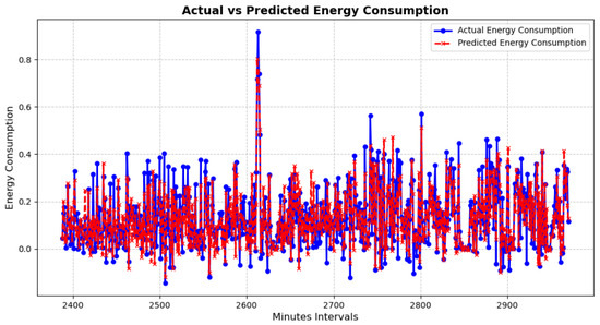
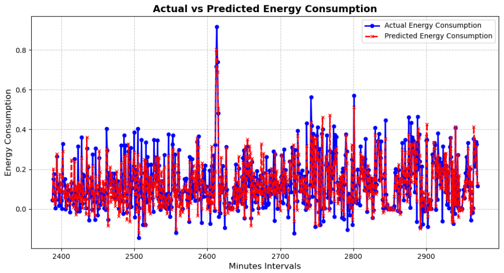
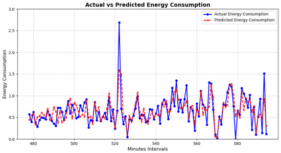
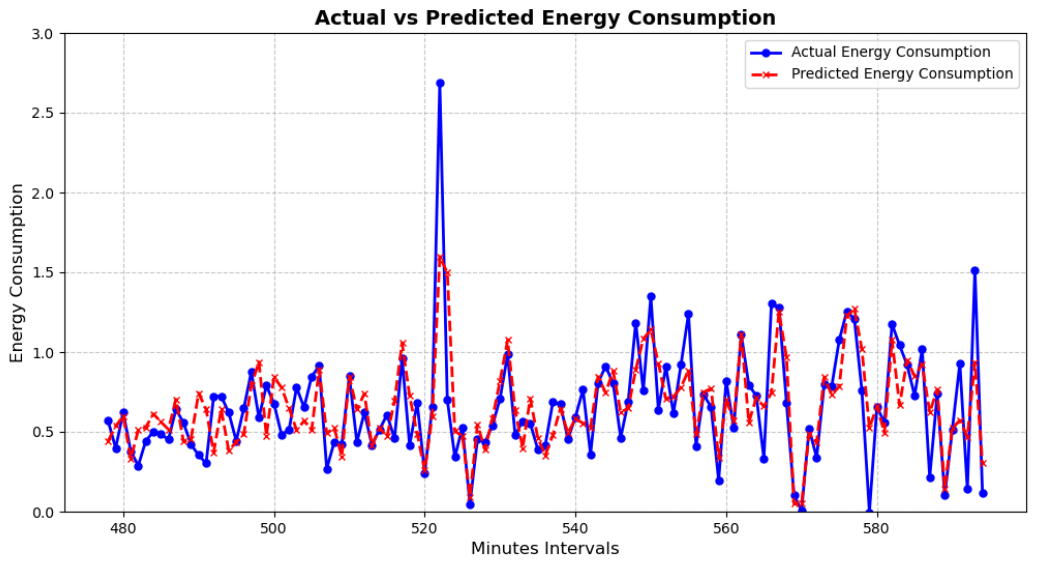
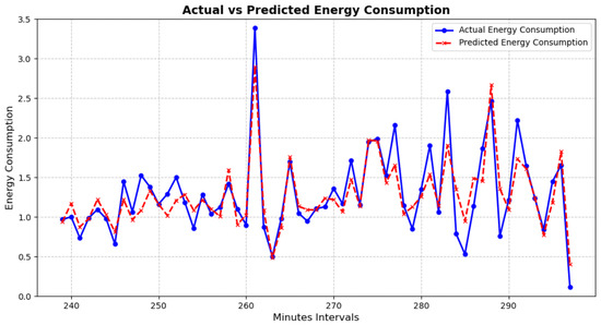
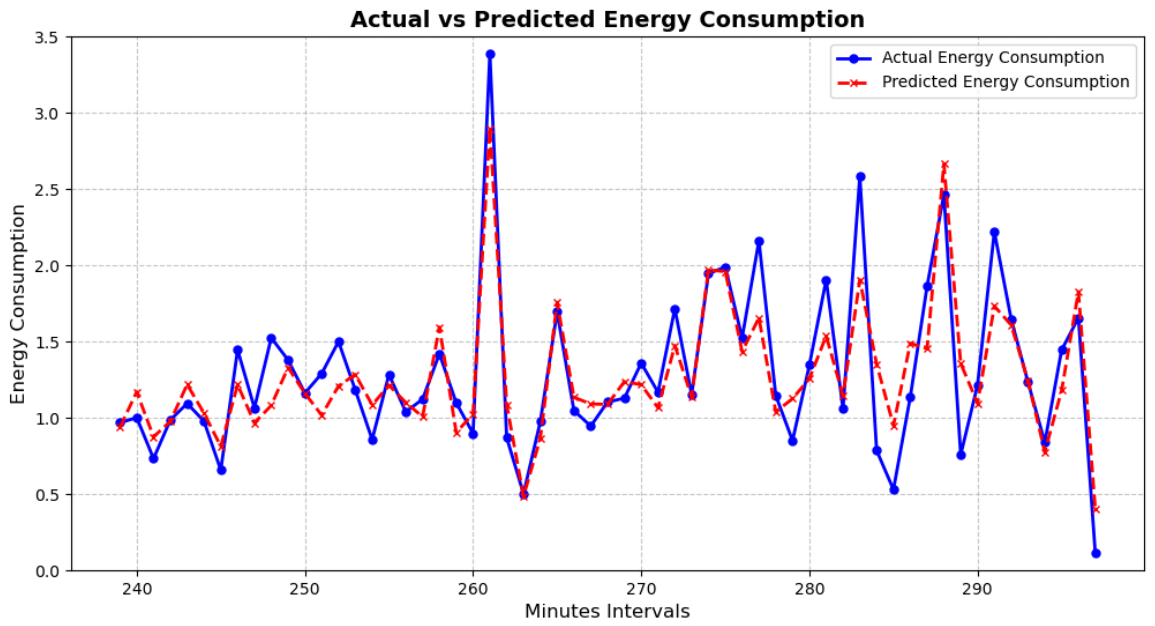
Among the nine evaluated model-input configurations, XGB-CL achieved the highest number of best metric values across the reported vehicle–interval cases, although its advantage over RF-ECL was limited. Therefore, XGB-CL was selected as a representative high-performing configuration for visualizing the predicted and actual energy consumption profiles. Figure 2, Figure 3 and Figure 4 illustrate the performance of the XGB-CL configuration for Vehicle 455 across the 1 min, 5 min, and 10 min temporal aggregation intervals, respectively. In all three cases, the predicted profiles follow the main trend of the actual energy consumption pattern, indicating that the combined use of energy consumption lags and external feature lags captures the underlying consumption dynamics effectively. At the 1 min interval, the actual profile exhibits stronger short-term fluctuations, which are expected in high-resolution EV data due to rapid changes in driving behavior, speed, acceleration/deceleration patterns, and auxiliary power demand. Nevertheless, the predicted curve remains close to the observed pattern, with deviations mainly appearing around abrupt changes in consumption.
Figure 2.
Predicted and actual energy consumption profiles for the XGB-CL configuration, Vehicle 455, at 1 min intervals.
Figure 3.
Predicted and actual energy consumption profiles for the XGB-CL configuration, Vehicle 455, at 5 min intervals.
Figure 4.
Predicted and actual energy consumption profiles for the XGB-CL configuration, Vehicle 455, at 10 min intervals.
At the 5 min and 10 min intervals, the effect of temporal aggregation becomes more evident, as the actual energy consumption lines become smoother and short-term variations are reduced. However, this smoothing does not appear to compromise the forecasting behavior of the model, since the predicted profiles remain well aligned with the actual curves and continue to capture the overall consumption trend. These visual results support the quantitative findings by showing that the XGB-CL configuration performs consistently across different temporal resolutions, capturing both fine-grained variability and smoother aggregated energy consumption patterns. Overall, the results demonstrate that no single model-input configuration dominates across all vehicles, temporal resolutions, and evaluation metrics. Nevertheless, XGBoost-based configurations, particularly XGB-CL and XGB-FL, achieved strong performance in several cases, with XGB-CL being the most frequently top-performing configuration among the nine evaluated model-input combinations. This justifies its selection as the representative configuration for visual analysis in Figure 2, Figure 3 and Figure 4, where the predicted profiles generally follow the actual energy consumption trends across the examined temporal aggregation intervals. Random Forest proved to be a reliable alternative, especially in configurations based on historical energy consumption lags, while Dynamic Linear Regression was competitive in selected cases, particularly at the 5 min interval for Vehicle 10. ARIMA-ECL generally underperformed compared with configurations that incorporated exogenous vehicle-related features, highlighting the limitations of relying exclusively on historical energy consumption values. These findings emphasize the importance of systematically evaluating multiple model families and lag-based input configurations, as forecasting performance depends on the interaction between vehicle behavior, temporal aggregation interval, input feature structure, and evaluation metric.
To contextualize the practical value of these numerical errors, the 1 min interval MAE values ranging between 0.04 and 0.09 kWh translate to a highly manageable cumulative error of approximately 2.4 to 5.4 kWh for an hour-long trip. For a typical EV equipped with a 60 to 80 kWh battery pack, this represents a range estimation uncertainty of only 3% to 7%, which significantly minimizes driver range anxiety and enables precise route planning and charging scheduling. Furthermore, the model’s robustness under extreme operating conditions is directly managed through its feature engineering design. Stop-and-go driving patterns and hilly terrains are addressed dynamically using statistical measures of transient acceleration and smoothed elevation, while auxiliary battery drains caused by extreme temperatures are also proactively modeled by incorporating OAT, heater power, and air-conditioning usage into the feature lag configurations, allowing the tree-based configurations to adaptively adjust predictions when auxiliary systems are heavily taxed, thus preserving forecasting accuracy across diverse environmental and topographical scenarios.
6. Discussion
While the proposed framework demonstrates robust forecasting performance, its practical implementation in charging scheduling and route planning requires a careful consideration of generalizability, prediction horizons, and scalability limits. In time-series forecasting, multi-step-ahead predictions are typically achieved through recursive models, which often suffer from compounding error propagation. To address longer forecasting horizons more reliably, this study directly models different temporal resolutions, including 1 min, 5 min, and 10 min intervals. This approach provides stable, physically representative forecasts over longer windows directly. Through these accurate predictions, EV users obtain immediate, actionable benefits, such as significantly reduced range anxiety via highly precise range estimation, the ability to select energy-optimized routes, and optimal thermal pre-conditioning of the cabin. Furthermore, aggregating these multi-horizon forecasts contributes to the more efficient management of charging infrastructure. By predicting aggregated EV energy demands, charging network operators can forecast peak loads on localized transformers, implement dynamic pricing, and schedule EV charging to align with periods of renewable energy generation on the grid. However, extending this direct forecasting approach beyond 10 min intervals presents a critical limitation related to dataset size, as aggregating data into larger temporal windows naturally reduces the sequence length, as resolutions exceeding 10 min (such as 20 min or 30 min steps) yield too few data points for robust model training, validation, and testing.
Similarly, deploying energy forecasting models across large-scale commercial fleets also presents challenges related to vehicle and driver heterogeneity, such as variations in payload, battery degradation, auxiliary power usage, and individual driving styles. Additional limitations can arise if the models are trained using data from only one geographic region or a specific vehicle type, as they cannot generalize to highly hilly terrains, distinct climate zones, or variations in vehicle mass, battery chemistry, and aerodynamic drag. Training a single centralized model for an entire fleet often degrades accuracy because generalized models struggle to capture these localized, vehicle-specific behaviors. The proposed energy forecasting framework also addresses this challenge by utilizing computationally lightweight models, such as XGBoost and Dynamic Linear Regression, which are suitable for decentralized deployment directly on edge-computing onboard vehicle systems, rather than relying on a heavy, centralized cloud architecture. Each vehicle can continuously run and update its own localized, highly customized model, matching the specific dynamics of the vehicle, its typical regional environment, and its driver. The primary challenge for this decentralized approach lies in establishing automated data pipelines on the vehicle’s edge computer to handle the temporal aggregation and real-time inference without degrading onboard processor performance.
Finally, to further enhance the proposed approach, incorporating real-time external data streams, including traffic conditions, weather forecasts, and the vehicle’s battery SoC, represents a promising direction. Real-time traffic data can provide immediate indicators of transient stop-and-go patterns that are not fully captured by historical lag structures. Similarly, incorporating live weather data, such as wind speed or precipitation, directly informs the model of fluctuating aerodynamic drag and wet road rolling resistance. Crucially, battery SoC significantly impacts energy consumption dynamics because battery internal resistance and regenerative braking capacity vary non-linearly with SoC (e.g., regenerative braking is limited when the battery is near full capacity). Therefore, integrating these dynamic real-world variables into the proposed lightweight, feature-lagged framework would enable proactive, highly adaptive adjustments to energy consumption baselines.
7. Conclusions
This research contributes to progress toward the SDGs, particularly in the context of sustainable transportation, by proposing a data-driven framework for improving energy consumption forecasting in electric vehicles. By supporting more accurate energy usage estimation, the proposed approach can contribute to more efficient EV operation, improved battery management, and the broader adoption of eco-friendly mobility solutions.
This study introduced a machine learning-based framework for predicting EV energy consumption using the eVED dataset. The proposed methodology combines preprocessing, temporal aggregation, statistical feature characterization, lag-based input configurations, and multiple forecasting models. By structuring the data into different temporal resolutions, namely 1 min, 5 min, and 10 min intervals, and by incorporating lagged representations of both historical energy consumption and external vehicle-related features, the framework enables the analysis of temporal dependencies under different driving and operating conditions.
The experimental results demonstrated that forecasting performance depends on the interaction between the model family, the lag-based input configuration, the temporal aggregation interval, and the vehicle-specific driving profile. No single model-input configuration consistently dominated across all vehicles, time resolutions, and evaluation metrics. Nevertheless, XGBoost-based configurations achieved strong performance in several cases, while XGB-CL, which combines historical energy consumption lags with external feature lags, was the most frequently top-performing configuration among the nine evaluated configurations. Random Forest also proved to be a reliable alternative, particularly in configurations based on historical energy consumption lags, while Dynamic Linear Regression showed competitive performance in selected cases. In contrast, ARIMA-ECL generally underperformed compared with configurations incorporating exogenous vehicle-related features, highlighting the limitations of relying exclusively on historical energy consumption values.
The findings indicate that integrating temporal aggregation, lag-based input construction, and machine learning can enhance EV energy consumption forecasting across different driving scenarios and vehicle characteristics. The 1 min interval provided the most detailed representation of short-term energy consumption variations, while the 5 min interval offered a practical balance between predictive accuracy and temporal abstraction. Such forecasting capabilities can support more effective energy management strategies, including eco-driving, optimized charging planning, and more reliable range estimation. Since range anxiety remains one of the major barriers to EV adoption, accurate energy consumption forecasts can help improve driver confidence and support the wider deployment of electric mobility solutions. Moreover, the analysis of external factors such as speed, acceleration, elevation, air-conditioning power, and heater power can provide useful insights into the operational conditions that influence EV energy demand.
Future work will focus on extending the proposed framework toward real-time deployment. In particular, real-time vehicle data streams, such as position, speed, acceleration, and auxiliary power usage, will be integrated to enhance the applicability of the methodology in dynamic environments. Within the context of the SINNOGENES project, the proposed approach will be further developed into a forecasting service for on-demand public transport operations. Given its strong overall performance, XGB-CL will be considered as the primary candidate configuration for this service, with future work evaluating its inference latency on edge-computing hardware to ensure onboard compatibility, while additional validation will be conducted under real-time operating conditions. The service will aim to forecast energy consumption for upcoming 1 min, 5 min, and 10 min intervals, facilitating the framework’s adaptation across different vehicle classes (e.g., passenger cars, buses, and trucks) through extensive fleet-wide validation under diverse operating conditions. Ultimately, the system will provide drivers or fleet operators with actionable information related to charging needs, energy management, and operational planning.
Author Contributions
Conceptualization, G.S., A.L., K.V. and D.T.; methodology, V.P., S.P. and G.S.; software, V.P. and S.P.; validation, V.P., G.S. and S.P.; investigation, V.P., G.S. and S.P.; data curation, V.P. and S.P.; writing—original draft preparation, V.P.; writing—review and editing, G.S., A.L., K.V. and D.T.; supervision, G.S.; project administration, G.S., A.L. and K.V.; funding acquisition, A.L., K.V. and D.T. All authors have read and agreed to the published version of the manuscript.
Funding
This work was funded by the European Union’s Horizon Europe project SINNOGENES (Storage innovations for green energy systems) under Grant Agreement No. 101096992.
Institutional Review Board Statement
Not applicable.
Informed Consent Statement
Not applicable.
Data Availability Statement
The data used in this study are available from the extended Vehicle Energy Dataset (eVED), as cited in the manuscript.
Acknowledgments
The authors acknowledge the use of OpenAI ChatGPT (model/version: GPT-5.5 Thinking, OpenAI, San Francisco, CA, USA) to support language editing, structural refinement, and the visual organization of Figure 1. All AI-assisted suggestions were reviewed, edited, and validated by the authors. The authors take full responsibility for the final content of the manuscript.
Conflicts of Interest
The authors declare no conflicts of interest.
References
- Østergaard, P.A.; Duic, N.; Noorollahi, Y.; Kalogirou, S. Renewable energy for sustainable development. Renew. Energy 2022, 199, 1145–1152. [Google Scholar] [CrossRef] [Scilit]
- Jose, P.S.; Natarajan, A.; Karthikeyan, S.; Bogaraj, T. Environmental and social impact of electric vehicles. In Advanced Technologies in Electric Vehicles; Elsevier: Amsterdam, The Netherlands, 2024; pp. 107–125. [Google Scholar]
- Sanguesa, J.A.; Torres-Sanz, V.; Garrido, P.; Martinez, F.J.; Marquez-Barja, J.M. A review on electric vehicles: Technologies and challenges. Smart Cities 2021, 4, 372–404. [Google Scholar] [CrossRef] [Scilit]
- Chen, T.; Zhang, B.; Pourbabak, H.; Kavousi-Fard, A.; Su, W. Optimal routing and charging of an electric vehicle fleet for high-efficiency dynamic transit systems. IEEE Trans. Smart Grid 2016, 9, 3563–3572. [Google Scholar] [CrossRef] [Scilit]
- Li, W.; Stanula, P.; Egede, P.; Kara, S.; Herrmann, C. Determining the main factors influencing the energy consumption of electric vehicles in the usage phase. Procedia Cirp 2016, 48, 352–357. [Google Scholar] [CrossRef] [Scilit]
- Alanazi, F. Electric vehicles: Benefits, challenges, and potential solutions for widespread adaptation. Appl. Sci. 2023, 13, 6016. [Google Scholar] [CrossRef] [Scilit]
- Akshay, K.; Grace, G.H.; Gunasekaran, K.; Samikannu, R. Power consumption prediction for electric vehicle charging stations and forecasting income. Sci. Rep. 2024, 14, 6497. [Google Scholar] [CrossRef] [Scilit] [PubMed]
- Gopinathan, N.; Shanmugam, P.K. Energy anxiety in decentralized electricity markets: A critical review on EV models. Energies 2022, 15, 5230. [Google Scholar] [CrossRef] [Scilit]
- Longo, M.; Zaninelli, D.; Viola, F.; Romano, P.; Miceli, R. How is the spread of the Electric Vehicles? In Proceedings of the 2015 IEEE 1st International Forum on Research and Technologies for Society and Industry Leveraging a Better Tomorrow (RTSI); IEEE: New York, NY, USA, 2015; pp. 439–445. [Google Scholar]
- Shethiya, A.S. Adaptive Learning Machines: A Framework for Dynamic and Real-Time ML Applications. Ann. Appl. Sci. 2024, 5. [Google Scholar]
- Klyuev, R.V.; Morgoev, I.D.; Morgoeva, A.D.; Gavrina, O.A.; Martyushev, N.V.; Efremenkov, E.A.; Mengxu, Q. Methods of forecasting electric energy consumption: A literature review. Energies 2022, 15, 8919. [Google Scholar] [CrossRef] [Scilit]
- Chudy-Laskowska, K.; Pisula, T. An Analysis of the Use of Energy from Conventional Fossil Fuels and Green Renewable Energy in the Context of the European Union’s Planned Energy Transformation. Energies 2022, 15, 7369. [Google Scholar] [CrossRef] [Scilit]
- Huang, H.; Li, B.; Wang, Y.; Zhang, Z.; He, H. Analysis of factors influencing energy consumption of electric vehicles: Statistical, predictive, and causal perspectives. Appl. Energy 2024, 375, 124110. [Google Scholar] [CrossRef] [Scilit]
- Petkevicius, L.; Saltenis, S.; Civilis, A.; Torp, K. Probabilistic deep learning for electric-vehicle energy-use prediction. In Proceedings of the 17th International Symposium on Spatial and Temporal Databases, Virtual, 23–25 August 2021; pp. 85–95. [Google Scholar]
- Hua, Y.; Sevegnani, M.; Yi, D.; Birnie, A.; McAslan, S. Fine-grained RNN with transfer learning for energy consumption estimation on EVs. IEEE Trans. Ind. Inform. 2022, 18, 8182–8190. [Google Scholar] [CrossRef] [Scilit]
- Athanasakis, E.; Spanos, G.; Papadopoulos, A.; Lalas, A.; Votis, K.; Tzovaras, D. A Comprehensive Leakage-Free Forecasting Pipeline for Segmented Time Series: Application to Cross-Trip State-of-Charge Prediction in Automated Electric Vehicles. IEEE Trans. Intell. Veh. 2024, 10, 5213–5228. [Google Scholar] [CrossRef] [Scilit]
- Chen, X.; Lei, Z.; Ukkusuri, S.V. Prediction of road-level energy consumption of battery electric vehicles. In Proceedings of the 2022 IEEE 25th International Conference on Intelligent Transportation Systems (ITSC); IEEE: New York, NY, USA, 2022; pp. 2550–2555. [Google Scholar]
- Tang, X.; Jia, T.; Hu, X.; Huang, Y.; Deng, Z.; Pu, H. Naturalistic data-driven predictive energy management for plug-in hybrid electric vehicles. IEEE Trans. Transp. Electrif. 2020, 7, 497–508. [Google Scholar] [CrossRef] [Scilit]
- Polymeni, S.; Pitsiavas, V.; Spanos, G.; Matthewson, Q.; Lalas, A.; Votis, K.; Tzovaras, D. Toward sustainable mobility: AI-enabled automated refueling for Fuel Cell Electric Vehicles. Energies 2024, 17, 4324. [Google Scholar] [CrossRef] [Scilit]
- Brooker, A.; Gonder, J.; Wang, L.; Wood, E.; Lopp, S.; Ramroth, L. FASTSim: A Model to Estimate Vehicle Efficiency, Cost and Performance; Technical report; SAE Technical Paper: Warrendale, PN, USA, 2015. [Google Scholar]
- Baratsas, S.; Iseri, F.; Pistikopoulos, E.N. A hybrid statistical and machine learning based forecasting framework for the energy sector. Comput. Chem. Eng. 2024, 188, 108740. [Google Scholar] [CrossRef] [Scilit] [PubMed]
- Zhang, Y.; Li, J.; Zhang, B.; Mao, M.; Qi, W.; Ye, X.; Hu, B. Internet-distributed energy management strategy for plug-in fuel cell hybrid electric vehicles considering power source degradation. IEEE Trans. Veh. Technol. 2025, 75, 9701–9715. [Google Scholar] [CrossRef] [Scilit]
- Zhou, X.; Li, J. Inverse Optimal Control for High-Order Nonlinear Fully Actuated Systems with Unknown Reward Weights. Int. J. Robust Nonlinear Control 2026, 36, 4674–4688. [Google Scholar] [CrossRef] [Scilit]
- Zhang, Y.; Li, J.; Wang, Y.; Xu, Q.; Zhang, X.; Gao, L.; Zhang, W.; Lai, F.; Miao, Y.; Tu, Y. A Multiple Loops-Based Control Strategy of Current Source Rectifier for Low-Voltage DC Distribution Systems. IEEE Trans. Ind. Appl. 2025, 62, 5860–5872. [Google Scholar] [CrossRef] [Scilit]
- Zhang, S.; Fatih, D.; Abdulqadir, F.; Schwarz, T.; Ma, X. Extended vehicle energy dataset (eVED): An enhanced large-scale dataset for deep learning on vehicle trip energy consumption. arXiv 2022, arXiv:2203.08630. [Google Scholar]
- Oh, G.; Leblanc, D.J.; Peng, H. Vehicle energy dataset (VED), a large-scale dataset for vehicle energy consumption research. IEEE Trans. Intell. Transp. Syst. 2020, 23, 3302–3312. [Google Scholar] [CrossRef] [Scilit]
- Mediouni, H.; Ezzouhri, A.; Charouh, Z.; El Harouri, K.; El Hani, S.; Ghogho, M. Energy consumption prediction and analysis for electric vehicles: A hybrid approach. Energies 2022, 15, 6490. [Google Scholar] [CrossRef] [Scilit]
- Yang, X.; Zhuge, C.; Shao, C.; Huang, Y.; Tang, J.H.C.G.; Sun, M.; Wang, P.; Wang, S. Characterizing mobility patterns of private electric vehicle users with trajectory data. Appl. Energy 2022, 321, 119417. [Google Scholar] [CrossRef] [Scilit]
- Spanos, G.; Giannoutakis, K.M.; Votis, K.; Viaño, B.; Augusto-Gonzalez, J.; Aivatoglou, G.; Tzovaras, D. A lightweight cyber-security defense framework for smart homes. In Proceedings of the 2020 International Conference on Innovations in Intelligent Systems and Applications (INISTA); IEEE: New York, NY, USA, 2020; pp. 1–7. [Google Scholar]
- Sun, Q.; Liu, J.; Rong, X.; Zhang, M.; Song, X.; Bie, Z.; Ni, Z. Charging load forecasting of electric vehicle charging station based on support vector regression. In Proceedings of the 2016 IEEE PES Asia-Pacific Power and Energy Engineering Conference (APPEEC); IEEE: New York, NY, USA, 2016; pp. 1777–1781. [Google Scholar]
- Saly, G.; Szauter, F.; Kocsis Szürke, S. Comprehensive Analysis of the Factors Affecting the Energy Efficiency of Electric Vehicles and Methods to Reduce Consumption: A Review. Eng. Proc. 2024, 79, 79. [Google Scholar] [CrossRef] [Scilit]
- Xiao, S.; Shao, Y.; Li, Y.; Yin, H.; Shen, Y.; Cui, B. LECF: Recommendation via learnable edge collaborative filtering. Sci. China Inf. Sci. 2022, 65, 112101. [Google Scholar] [CrossRef] [Scilit]
- Meire, M.; Ballings, M.; Van den Poel, D. The added value of auxiliary data in sentiment analysis of Facebook posts. Decis. Support Syst. 2016, 89, 98–112. [Google Scholar] [CrossRef] [Scilit]
- Aivatoglou, G.; Anastasiadis, M.; Spanos, G.; Voulgaridis, A.; Votis, K.; Tzovaras, D. A tree-based machine learning methodology to automatically classify software vulnerabilities. In Proceedings of the 2021 IEEE International Conference on Cyber Security and Resilience (CSR); IEEE: New York, NY, USA, 2021; pp. 312–317. [Google Scholar]
- Aivatoglou, G.; Anastasiadis, M.; Spanos, G.; Voulgaridis, A.; Votis, K.; Tzovaras, D.; Angelis, L. A RAkEL-based methodology to estimate software vulnerability characteristics & score-an application to EU project ECHO. Multimed. Tools Appl. 2022, 81, 9459–9479. [Google Scholar] [CrossRef] [Scilit]
- Rathore, H.; Meena, H.K.; Jain, P. Prediction of ev energy consumption using random forest and xgboost. In Proceedings of the 2023 International Conference on Power Electronics and Energy (ICPEE); IEEE: New York, NY, USA, 2023; pp. 1–6. [Google Scholar]
- Breiman, L. Random forests. Mach. Learn. 2001, 45, 5–32. [Google Scholar] [CrossRef] [Scilit]
- Chen, T.; Guestrin, C. Xgboost: A scalable tree boosting system. In Proceedings of the 22nd ACM Sigkdd International Conference on Knowledge Discovery and Data Mining, San Francisco, CA, USA, 13–17 August 2016; pp. 785–794. [Google Scholar]
- Pankratz, A. Forecasting with Dynamic Regression Models; John Wiley & Sons: Hoboken, NJ, USA, 2012. [Google Scholar]
- Makridakis, S.; Spiliotis, E.; Assimakopoulos, V. Statistical and Machine Learning forecasting methods: Concerns and ways forward. PLoS ONE 2018, 13, e0194889. [Google Scholar] [CrossRef] [Scilit] [PubMed]
- Wang, Z.; Wang, Y.; Zeng, R.; Srinivasan, R.S.; Ahrentzen, S. Random Forest based hourly building energy prediction. Energy Build. 2018, 171, 11–25. [Google Scholar] [CrossRef] [Scilit]
- Pang, X.; Luan, C.; Liu, L.; Liu, W.; Zhu, Y. Data-driven random forest forecasting method of monthly electricity consumption. Electr. Eng. 2022, 104, 2045–2059. [Google Scholar] [CrossRef] [Scilit]
- Chujai, P.; Kerdprasop, N.; Kerdprasop, K. Time series analysis of household electric consumption with ARIMA and ARMA models. In Proceedings of the International Multiconference of Engineers and Computer Scientists, Hong Kong, 13–15 March 2013; Volume 1, pp. 295–300. [Google Scholar]
- Moslemi, Z.; Clark, L.; Kernal, S.; Rehome, S.; Sprengel, S.; Tamizifar, A.; Tuli, S.; Chokshi, V.; Nomeli, M.; Liang, E.; et al. Comprehensive Forecasting of California’s Energy Consumption: A Multi-Source and Sectoral Analysis Using ARIMA and ARIMAX Models. arXiv 2024, arXiv:2402.04432. [Google Scholar]
- Liashchynskyi, P.; Liashchynskyi, P. Grid search, random search, genetic algorithm: A big comparison for NAS. arXiv 2019, arXiv:1912.06059. [Google Scholar]
- Hyndman, R.J.; Koehler, A.B. Another look at measures of forecast accuracy. Int. J. Forecast. 2006, 22, 679–688. [Google Scholar] [CrossRef] [Scilit]
- Polymeni, S.; Spanos, G.; Tsiktsiris, D.; Athanasakis, E.; Votis, K.; Tzovaras, D.; Kormentzas, G. everWeather: A Low-Cost and Self-Powered AIoT Weather Forecasting Station for Remote Areas. In Environmental Informatics; Springer: Berlin/Heidelberg, Germany, 2023; pp. 141–158. [Google Scholar]

Disclaimer/Publisher’s Note: The statements, opinions and data contained in all publications are solely those of the individual author(s) and contributor(s) and not of MDPI and/or the editor(s). MDPI and/or the editor(s) disclaim responsibility for any injury to people or property resulting from any ideas, methods, instructions or products referred to in the content. |
© 2026 by the authors. Licensee MDPI, Basel, Switzerland. This article is an open access article distributed under the terms and conditions of the Creative Commons Attribution (CC BY) license.