


Abstract
This paper examines whether the relationships between environmentally related taxes, environmental outcomes, and environmental protection expenditures are more consistent with the environmental objectives emphasised by Pigouvian approaches or with a predominantly revenue-raising role of environmental taxation in 27 OECD economies over the period 1995–2023. To address this question, two complementary models are estimated: the first examines the effects of environmental taxes and environmental protection expenditures on the ecological footprint, while the second examines the long-run relationship between environmental tax revenues and environmental protection expenditures. Pedroni and Westerlund tests provide evidence of long-run relationships in both models. BA-OLS and CUP-FM estimates show that environmental taxes reduce the ecological footprint, although their average effect is statistically insignificant, whereas environmental protection expenditures significantly reduce it. Environmental taxes also have a positive and significant effect on environmental protection expenditures. The MMQR results reveal substantial heterogeneity underlying these average relationships. The negative effect of environmental taxes on the ecological footprint becomes progressively stronger as the ecological footprint increases and is significant from the median to the upper quantiles, whereas the effect of environmental protection expenditures remains statistically insignificant across all quantiles. In the second model, the positive effect of environmental taxes on environmental protection expenditures is significant only in the middle quantiles, indicating that the positive relationship between environmental tax revenues and environmental protection expenditures is not uniform across the distribution. Taken together, the findings provide conditional support for the Strict Pigouvian Approach and partial support for the Broad Pigouvian Approach: environmental taxes are more effective in reducing ecological footprints at higher levels of environmental pressure, while their positive association with environmental protection expenditures is not uniform across the distribution.
1. Introduction
Increasing environmental pollution and climate change have emerged as major global challenges, posing serious risks to ecological balance, economic sustainability, and human well-being [1,2]. Therefore, combating environmental pollution and climate change is considered a multidimensional process that is not limited to the national policy choices of individual countries but also requires international cooperation and coordination. In this context, the 2015 Paris Agreement, one of the most important international initiatives aimed at establishing common global climate targets, seeks to maintain the global average temperature increase at a level well below 2 °C above pre-industrial levels and, if possible, to keep the increase within 1.5 °C [3]. It is emphasised that achieving these goals will require global greenhouse gas (GHG) emissions to decline by around 45% by 2030 and to reach net-zero emissions by 2050 [4]. However, current assessments indicate that existing policies are insufficient to achieve these goals. According to projections by the UN Environment Programme [5], if current policies continue, global GHG emissions are expected to exceed the levels consistent with the Paris Agreement targets by 2030. Similarly, the Global Footprint Network [6] reports that global ecological demand has long exceeded the Earth’s biocapacity by around 75%. These findings indicate that achieving the Paris Agreement targets will become increasingly difficult if current trends persist and highlight the growing need for more effective and sustainable policy instruments to mitigate environmental degradation.
Achieving environmental goals depends not only on technological developments and voluntary practices, but also on implementing economic policy tools effectively to internalise environmental externalities. The inability of the market mechanism to fully reflect environmental costs in prices necessitates public intervention; in this context, environmental taxes (hereafter ENVTAX) stand out as one of the most important market-based environmental policy instruments. The theoretical basis of this approach rests on [7] theory of externalities. According to Pigou, the failure to reflect negative externalities arising from production and consumption activities in the price mechanism impairs resource allocation efficiency and leads to excessive environmental degradation. Therefore, ENVTAX aim to internalize externalities by shifting the costs imposed on society by polluting activities back to the polluters, and to guide economic decision-makers towards more environmentally friendly production and consumption patterns [8]. Effectively designed ENVTAX can not only reduce environmental pressures but also contribute to sustainable economic transformation by promoting low-carbon production technologies [9,10,11].
ENVTAX are implemented in practice through various instruments, such as energy taxes, transportation taxes, and pollution and natural resource taxes, ensuring pricing of environmental costs within the economic system in accordance with the “polluter pays” principle. In this respect, ENVTAX are regarded as one of the key policy tools for achieving the emission reduction targets set under the Paris Agreement. However, there is no complete consensus in the literature relating to the theoretical foundations and the basic function of ENVTAX in practice. These discussions revolve around the question of what purpose ENVTAX should serve. Different theoretical approaches have been developed regarding whether the main purpose of ENVTAX is to correct environmental externalities, to redirect tax revenues to environmental purposes, to increase economic efficiency, or to increase public revenues [9,12,13]. These discussions are generally addressed within four main theoretical frameworks: the Strict Pigouvian Approach (SPA), the Broad Pigouvian Approach, the Double Dividend Hypothesis (DDH), and the Fiscal Leviathan Approach (FLA). These approaches put forward different assumptions about the purpose of ENVTAX, the way tax revenues are used, and their role in public finance.
According to the first approach, the Strict Pigouvian Approach, the primary aim of ENVTAX is to reduce polluting activities and increase societal well-being by internalizing environmental externalities. In this approach, effectively designed ENVTAX are considered sufficient to correct environmental externalities, while redirecting the resulting tax revenues to environmental purposes is not considered a necessary element [9,13]. In contrast, the Broad Pigouvian Approach argues that, due to the complex nature of environmental problems, taxation alone is insufficient, and that using the revenues from ENVTAX in conjunction with environmental protection expenditures (hereafter EPE) and other environmental policies will increase environmental effectiveness [13,14,15]. According to this approach, the success of ENVTAX depends not only on reducing polluting activities but also on the allocation of the resulting revenues to environmental purposes.
In contrast to Pigouvian approaches, the DDH suggests that ENVTAX not only improve environmental quality but also provide additional public revenue, contributing to the reduction in existing distortionary taxes, the financing of public spending, or the support of environmental investments [12,16,17]. According to this approach, the second benefit provided by ENVTAX depends not only on the collection of tax revenues but also on how these revenues are utilized in the economy [18]. Indeed, ref. [19] emphasize that the second benefit does not automatically arise from the existence of ENVTAX but rather depends on the reduction in other distortionary taxes or the allocation of tax revenues to areas that will increase social welfare. Therefore, in evaluating the effectiveness of ENVTAX, the way the tax revenues are allocated, as well as the environmental consequences of the tax, stands out as one of the key determinants.
Fourthly, the FLA, based on public choice theory, argues that ENVTAX may not always serve environmental purposes in practice. According to this approach, governments could use ENVTAX as a tool to raise fiscal revenue because they are more readily accepted by public compared to other taxes and allocate the resulting revenues to general budget funding or political priorities instead of environmental targets [13,17,20]. Therefore, the success of ENVTAX should be evaluated not only from the perspective of environmental improvement but also from the perspective of the intended use of tax revenues. This necessitates questioning the fundamental motivation behind ENVTAX.
These four approaches differ mainly in the objectives attributed to environmental taxes and in the way tax revenues are expected to be used. Consequently, whether ENVTAX primarily pursue environmental objectives or revenue-generating motives remains an open empirical question.
At this point, focusing solely on environmental quality indicators may provide an incomplete picture of the role of ENVTAX in environmental fiscal policy. It is also important to consider the relationship between environmental tax revenues and environmental protection expenditures. It is also necessary to consider how the revenues from these taxes are used within the public budget. In the public finance literature, the allocation of revenues from a particular tax to expenditures within the same policy area is explained by the earmarking (or hypothecation) approach. Ref. [21] argue that, especially in situations of political uncertainty and intergovernmental policy differences, allocating environmental tax revenues to environmental purposes can strengthen the continuity of environmental policy commitments by limiting the redirection of these revenues to different fiscal objectives. Within this framework, the earmarking approach for ENVTAX argues that using the revenues generated to finance EPE can strengthen the environmental legitimacy and public acceptance of these taxes. In this context, public expenditures such as environmental infrastructure investments, waste management, environmental R&D activities, and similar initiatives can contribute to improving environmental quality by playing a complementary role in addressing market failures [22,23,24,25,26,27]. Conversely, the inclusion of environmentally related tax revenues within the general budget and their insufficient allocation to environmental objectives strengthens criticisms that the revenue-generating function of these taxes outweighs their environmental benefits. Therefore, the fact that ENVTAX support EPE in addition to reducing the carbon footprint can be considered consistent with both the Broad Pigouvian Approach and the DDH. Conversely, a limited relationship between ENVTAX and either environmental quality or EPE would provide weaker empirical consistency with the environmental objectives emphasised by Pigouvian approaches.
Considering these discussions, OECD countries provide an appropriate setting for this study because ENVTAX have been implemented for many years within well-established environmental fiscal policy frameworks. In these economies, the main policy debate no longer concerns whether environmental taxes should be introduced, but rather how the resulting revenues should be used. As noted by the [17], these revenues may finance environmental protection, reduce distortionary taxes, or support general public expenditures. This makes OECD countries an appropriate setting for assessing not only the environmental effectiveness of ENVTAX but also the relationship between environmental tax revenues and EPE.
In the literature, the effectiveness of ENVTAX is largely evaluated through their impact on carbon emissions, carbon footprint, or other environmental quality indicators. However, studies that directly question whether ENVTAX are implemented for environmental purposes or with the motivation of generating fiscal revenue are quite limited. In particular, the relationship between the environmental consequences of ENVTAX and environmental protection expenditures represents a significant gap in the literature. The main aim of this study is to examine whether the observed relationships between environmental taxes, environmental outcomes, and environmental protection expenditures are more consistent with the environmental objectives emphasized by Pigouvian approaches or with a predominantly revenue-raising role of environmental taxation. To address this question, two complementary models are estimated using panel data for 27 OECD countries covering the period 1995–2023. The first model evaluates the environmental effectiveness of ENVTAX by examining their effects on the ecological footprint (EFP), while the second examines the long-run relationship between environmental tax revenues and environmental protection expenditures (EPE). Long-run relationships are examined using the [28,29,30] panel cointegration tests, followed by BA-OLS, CUP-FM and MMQR estimators. By combining these two models with both linear and nonlinear estimation techniques, the study provides new evidence on the environmental effectiveness of ENVTAX and their long-run relationship with environmental protection expenditures.
Beyond the linear and quantile-based econometric framework, this paper reports a set of functional-form diagnostics comprising four linear benchmarks (OLS, Ridge, LASSO, and Elastic Net) and seven flexible learners (Support Vector Regression, k-Nearest Neighbors, Random Forest, Extra Trees, Gradient Boosting, Artificial Neural Networks, and Generalized Additive Models). These diagnostics assess whether a specification that is linear in parameters is adequate for the data and thereby inform the choice of estimator; they are not intended to validate the MMQR coefficients or to establish causal effects. Such an assessment of functional form is rarely undertaken alongside parametric estimation in the environmental tax literature. The evidence bearing directly on the estimated parameters is provided separately by a battery of MMQR diagnostic tests rarely reported together in prior studies, including the scale relevance (Wald) test, the location-scale specification test, the distributional fixed effects test, and a scale positivity control test. Because the quantile coefficients in this framework are given by β(τ) = β + q(τ)γ, the scale relevance test is defined on the estimated parameters themselves and provides direct econometric evidence on whether the effects vary across the conditional distribution. By combining functional-form diagnostics with these parameter-based tests, the study offers a methodologically more rigorous and transparent empirical foundation than conventional single-method approaches in this strand of the literature.
2. Literature Review
2.1. ENVTAX, EPE, and Environmental Quality Nexus
ENVTAX and EPE are among the most commonly used fiscal instruments of environmental policy, and their effects on environmental health have attracted substantial attention in the literature. However, empirical studies have not reached a common conclusion regarding the effects of ENVTAX and EPE on environmental indicators. The findings vary considerably depending on the country groups studied, the environmental quality indicators used, policy design, institutional structure, and the econometric methods applied. Therefore, the literature presents a highly heterogeneous picture regarding the environmental effectiveness of these policy instruments.
A substantial body of studies addressing the effect of ENVTAX on environmental health shows that these taxes mitigate emissions and environmental degradation by making polluting activities more costly. Early studies by [31,32,33,34,35] demonstrated that ENVTAX contribute to emission reduction and improved environmental performance. Later studies have highlighted nonlinear relationships and threshold effects. In this context, refs. [11,36] showed that environmental improvement becomes more pronounced when ENVTAX exceed a certain threshold. Similarly, refs. [37,38,39,40,41,42,43,44] using different country samples and econometric techniques, show that ENVTAX have beneficial effects on environmental sustainability by mitigating pollutant emissions. For EU countries, ref. [13] found that ENVTAX are effective in reducing pollutant emissions and that governments mainly use these taxes in a manner consistent with the Pigouvian approach; furthermore, their findings regarding the use of environmental tax revenues as a substitute for other distortionary taxes provided limited empirical support for the DDH. These findings generally indicate that ENVTAX, if appropriately designed, can be an effective fiscal tool in achieving environmental goals.
On the other hand, there are also studies in the literature revealing that ENVTAX do not always produce the expected environmental results. Refs. [45,46,47,48,49,50,51,52] have shown that ENVTAX have had limited or statistically insignificant effects on environmental indicators in some countries and periods. For Western and Central European countries, ref. [53] showed that stringent environmental policies significantly reduced GHG emissions only in Western European countries, while ENVTAX had no significant effect in either region. The study also emphasized that R&D expenditures were the strongest determinant of emission reduction in Western and Central European countries. Similarly, ref. [50] showed that ENVTAX do not create a significant environmental impact in the overall OECD sample, but their effects on reducing carbon and GHG emissions are more pronounced in EU member states within the OECD. The effectiveness of ENVTAX depends not only on their implementation but also on factors such as tax rates, policy design, institutional quality, governance capacity, and energy structure. Supporting this view, ref. [54] found that energy taxes largely support the DDH in Scandinavian countries but not in G7 economies. Likewise, ref. [55] reported stronger support for the DDH in older EU member states, whereas environmental and economic gains remained more limited in newer member states. Ref. [56] further showed that the emission-reducing effect of ENVTAX is stronger in countries with high governance quality, strong democratic institutions, and low political corruption. Together, these findings indicate that the environmental effectiveness of ENVTAX is shaped by countries’ institutional and structural characteristics.
When examining the relationship between EPE and environmental quality, similarly varying results are encountered. Refs. [44,57,58,59,60,61] demonstrate that public EPE improve environmental health by reducing the EFP and GHG emissions. Ref. [61] also show that digital finance strengthens the emission-reducing effect of EPE, and that this effect differs between regions. Similarly, ref. [62], in a spatial econometric analysis conducted across 20 local governments in Taiwan, found that EPE significantly reduced air pollution; furthermore, the study showed that environmental protection subsidies provided by the central government were more effective in improving air quality than local government expenditures. Ref. [63], in a panel data analysis covering 117 countries, revealed that EPE are effective in reducing GHG emissions; however, the study emphasised that the effectiveness of environmental expenditures should be supported by proper budgeting, reporting, and implementation capacity. In contrast, refs. [64,65,66] show that the impact of EPE on environmental indicators is not always positive; the effectiveness of these expenditures depends on resource allocation, implementation capacity, the time dimension, and policy design. These findings reveal that the areas to which expenditures are directed and the extent to which they are used effectively are more decisive than the magnitude of EPE.
Overall, empirical findings regarding both ENVTAX and EPE are far from reaching a common conclusion. While a significant proportion of studies report that these policy instruments improve environmental quality, others find their effects to be limited or insignificant. Existing evidence suggests that their effectiveness depends on country-specific factors, including taxation levels, revenue allocation, institutional quality, governance capacity, and policy design. In support of this view, refs. [67,68] provide evidence in favour of the DDH, showing that environmental and economic gains are more likely when environmental tax revenues are directed towards environmental investments or the reduction in distortionary taxes. However, most existing studies examine the effects of ENVTAX and EPE separately, and empirical analyses evaluating both policy instruments within a unified framework remain limited. This gap highlights the need for further research to jointly assess the environmental effectiveness of ENVTAX and their relationship with EPE.
2.2. Environmental Tax Revenues and EPE Nexus
Although the impacts of ENVTAX on environmental well-being have been widely studied in the literature, empirical studies examining the relationship between environmental tax revenues and EPE are relatively limited. Existing studies mainly examine the purposes for which environmental tax revenues are used and whether these revenues are allocated to environmental purposes.
In this framework, ref. [69] explored the purpose of ENVTAX in the EU-28 within the framework of the Pigouvian and Leviathan approaches. The findings obtained using the Arellano–Bond dynamic panel GMM method reveal that environmental tax rates are effectively reducing GHG emissions and that ENVTAX are predominantly used for Pigouvian purposes. In contrast, no significant findings were obtained regarding the allocation of ENVTAX to social protection and general public service expenditures, thus failing to provide empirical evidence supporting the Leviathan approach. Ref. [13], on the other hand, evaluated the purpose of ENVTAX for the same group of countries within the framework of the Strict Pigouvian Approach, the Broad Pigouvian Approach, the DDH, and the FLA. While the study determined that environmental tax rates support the Strict Pigouvian Approach by reducing GHG emissions, no significant relationship was found between ENVTAX and EPE. Therefore, the Broad Pigouvian Approach, which suggests that ENVTAX are systematically allocated to environmental purposes, was not supported. Furthermore, while there is limited evidence that ENVTAX can be used as a substitute for personal income taxes, empirical evidence supporting the Leviathan approach was not found.
Studies directly addressing the impacts of revenue from environmental taxes on EPE have yielded differing results. Ref. [70] investigated the allocation of ENVTAX to EPE in EU countries and found that a significant portion of ENVTAX was not allocated to EPE. However, a strong and positive relationship was found among ENVTAX and EPE. Nevertheless, it was emphasised that this relationship does not imply causality and that an increasing need for environmental protection can also increase ENVTAX. Similarly, ref. [71] examined the relationship between ENVTAX and EPE using data covering the period 2008–2018 for Turkey and 30 European countries. The findings show that a stable and long-term relationship could not be established between ENVTAX and EPE. The study also determined that environmental tax shocks positively affected EPE only in the short term; this indicates that ENVTAX are not systematically allocated to EPE, and that this relationship largely depends on the fiscal policy choices implemented. Similarly, ref. [72], in their panel data analysis of 11 EU countries, determined that ENVTAX positively and significantly increased EPE. However, they found that the increase in EPE lagged the increase in ENVTAX, and that the impact of total government expenditures on EPE was stronger. Therefore, the study highlights that ENVTAX are not adequately allocated to environmental targets and that the effectiveness of current environmental fiscal policies needs to be improved.
There are also studies in the literature that demonstrate that the use of ENVTAX is decisive in the success of environmental fiscal policies. Ref. [68] examined whether environmental fiscal reforms could achieve the DDH in the Tunisian economy using a dynamic CGE-OLG model. Simulation results show that when ENVTAX are allocated to general public expenditures, economic and environmental gains cannot be achieved simultaneously. In contrast, the direct allocation of ENVTAX to pollution reduction activities both improves environmental quality and increases economic well-being, thus supporting the DDH. These findings show that the success of ENVTAX depends not only on the implementation of the tax but also on how the resulting revenues are allocated.
Overall, empirical findings regarding the reflection of ENVTAX on EPE are limited, and a consensus is lacking. While some studies show that ENVTAX are allocated to environmental purposes, others suggest that these revenues are largely used within the general budget or reflected in EPE only to a limited extent. Furthermore, while a significant portion of the literature assesses the allocation of ENVTAX through theoretical or indirect indicators, studies empirically examining the direct relationship between ENVTAX and EPE are quite limited. This situation highlights the need for further empirical evidence on the relationship between ENVTAX, environmental outcomes, and EPE.
3. Data & Model
This study analyses the impact of ENVTAX and EPE on demand-driven environmental footprints using annual panel data from 27 OECD economies (Austria, Belgium, Czech Republic, Denmark, Estonia, Finland, France, Germany, Greece, Hungary, Israel, Italy, South Korea, Latvia, Lithuania, Luxembourg, Netherlands, Norway, Poland, Portugal, Slovakia, Slovenia, Spain, Sweden, Switzerland, and the United Kingdom) covering the period 1995–2023; it also examines how environmental protection expenditures are shaped by environmental taxes, government spending, GDP per capita, and industry share. The demand-driven EFP data used in the study was obtained annually from the Global Footprint Network database. Data on environmental taxes were obtained from the OECD Data database and are expressed in per capita terms, so that the scaling of the tax variable is consistent with that of the dependent variables. The panel is balanced: 27 countries observed annually over 1995–2023 give 783 observations, with no missing values for any variable. Data on general government environmental protection expenditure (percentage of GDP), urban population, energy use (kg oil equivalent per capita), trade openness [(exports + imports)/GDP, %], and GDP per capita (2015 constant US dollars) were obtained from the World Bank database. Table 1 presents the definitions, units of measurement, data sources, and model specifications for the variables employed in this study.
Table 1.
Definition of variables.
The study examines different dimensions of environmental policies using two separate models. The first model aims to reveal the effects of ENVTAX and EPE on the demand-driven environmental footprint, while the second model examines how environmental protection expenditures are shaped by environmental taxes and selected macroeconomic indicators.
In the equations, EFP represents the demand-based ecological footprint (gha per person); ENVTAX represents environmental taxes (million USD per capita); and EPE represents general government environmental protection expenditure (percentage of GDP). The explanatory variables are defined as URB (urban population), EUSE (energy use per capita, kg oil equivalent), TRADE (trade openness, exports + imports as a percentage of GDP, %) and GDPPC (GDP per capita, 2015 constant US dollars). In the equations, i represents the country index, t represents the time dimension (years), and ε represents the error term. Two different dependent variables were used in the study. In the first model, the demand-driven ecological footprint was used as the dependent variable, and in the second model, environmental protection expenditures were used.
4. Methodology
This study is conducted for 27 OECD countries using annual data covering the period 1995–2023. The inclusion of OECD countries in the sample was influenced by the relatively more developed and institutionalised environmental policies in these countries, as well as the widespread application of ENVTAX as a policy tool. Furthermore, the continuity and accessibility of the datasets were considered as key criteria in country selection. The increased trade and financial integration between countries due to globalization can cause economies to be simultaneously affected by common external shocks [73]. This situation can lead to inter-cross-sectional dependence in panel data analysis, affecting the reliability of the estimation results. Indeed, ref. [74] states that ignoring cross-sectional dependence can increase the probability of incorrectly rejecting the null hypothesis. Therefore, testing for the presence of cross-sectional dependence is an important prerequisite before starting panel data analysis. For this purpose, the [75] CD test, which establishes the null hypothesis that there is no cross-sectional dependence, is applied. If cross-sectional dependence is not detected according to the test results, first-generation panel unit root tests can be used; however, if cross-sectional dependence is present, it is recommended to use second-generation panel unit root tests [73].
Since cross-sectional dependence was detected for most variables, second-generation panel unit root tests were employed. Among these, the PANIC test developed by [76] was selected because it separates common and idiosyncratic components of the series, allowing stationarity to be evaluated while accounting for common shocks across cross-sectional units. This feature makes the test particularly suitable for panel datasets characterised by cross-sectional dependence [77]. Previous studies also report that the PANIC approach provides more reliable results than alternative second-generation unit root tests when cross-sectional dependence is driven by common dynamic factors [78]. Since the PANIC test could not be implemented for the EPE variable, the Levin–Lin–Chu (LLC) and Hadri unit root tests were additionally employed.
The Westerlund cointegration test (2005), used to determine long-term relationships in panel data analysis, assumes that there is no cointegration relationship among the series. However, considering heterogeneity is important because dynamic structures and error variances can differ between cross-sections in panel datasets. In this regard, the heterogeneous panel cointegration test developed by [28,29] allows for the analysis of long-term relationships within a more flexible framework by acknowledging the presence of different individual effects between cross-sections [79].
Since the [75] CD test rejects the null of cross-sectional independence for all series, long-run coefficient estimators that ignore this dependence can be inconsistent. Following [80], the dependence is modelled through an unobserved common factor structure, in which the error term of the cointegrating regression is decomposed into a set of unobserved global stochastic trends, their country-specific loadings, and an idiosyncratic component. The number of common factors is determined by an information criterion [81]; in our analysis two common factors are selected for both models.
Under this error structure, pooled OLS remains consistent but suffers from a second-order asymptotic bias, so that inference based on it is invalid. Ref. [80] therefore propose a two-step fully modified procedure in which the common factors are extracted from the first-stage OLS residuals and the resulting bias is removed analytically, yielding the bias-adjusted OLS (BA-OLS) estimator. Because this estimator conditions on first-stage estimates of the factor structure, ref. [82] develop the continuously updated fully modified (CUP-FM) estimator, which instead iterates between the estimation of the long-run coefficients and the estimation of the factors and loadings until convergence. Thus, the correction for endogeneity and serial correlation is updated at every step rather than fixed at the first stage. Both estimators are consistent and asymptotically normal and permit inference using standard test statistics, while the Monte Carlo evidence reported by [80,82] indicates that CUP-FM exhibits smaller bias and superior small-sample properties relative to the two-step and OLS alternatives, and remains robust to endogeneity, serial correlation and heteroskedasticity. CUP-FM is accordingly adopted as the preferred estimator, with BA-OLS reported alongside it for comparison. This combination of BA-OLS and CUP-FM has previously been applied to cross-sectionally dependent panels by [83,84].
Traditional linear panel estimators focus on the conditional mean and assume that the effects of explanatory variables remain constant across the distribution of the dependent variable. However, economic relationships may vary under different environmental and institutional conditions, making mean-based estimators insufficient to capture such heterogeneity [27]. To address this issue, the Method of Moments Quantile Regression (MMQR) proposed by [82] was employed. Unlike conventional panel estimators, MMQR allows coefficient estimates to vary across different quantiles while incorporating individual fixed effects, thereby providing a more flexible framework for analysing heterogeneous relationships. The method is also less sensitive to outliers and distributional asymmetries, making it well suited to the heterogeneous characteristics of OECD countries.
While traditional econometric methods generally rely on the assumption that the relationship between variables is linear, machine learning approaches can reveal complex structures in data without the need for such restrictive assumptions. These methods offer the possibility of modeling nonlinear relationships, interactions between variables, and heterogeneous effects between observations with a flexible and data-driven approach [85].
When certain assumptions are included in the learning process, the modeling process can be significantly simplified. However, these assumptions can also limit the scope of relationships that can be identified. Algorithms that rely on reducing the function structure to a predetermined linear form are called linear models. Methods such as linear regression (LR) and logistic regression can be given as examples of this class. In this study, four linear models were evaluated: Ridge, Least Absolute Reduction and Selection Operator (LASSO), Elastic Net (EN) which adds regularization penalties to the loss function during the training process, and finally OLS. Linear models are used as a basic benchmark in evaluating the performance of other machine learning algorithms [86].
Algorithms that do not have strong assumptions about the structure of the mapping function are defined as nonlinear models. Support Vector Regression (SVR) and k-Nearest Neighbors (KNN) algorithms are examples of this class. These models are often used effectively in the analysis of datasets with many interrelated features. In this context, SVR is a regression algorithm based on the support vector approach and provides successful results especially in modeling non-linear relationships. The KNN algorithm can be used in both classification and regression problems. In classification problems, the KNN algorithm attempts to predict the class to which an observation belongs by considering local probabilities, while in regression problems, it estimates the value of the output variable based on local means. One of the most important advantages of machine learning methods is their ability to work effectively with nonlinear data structures [86,87]. The KNN assignment method is a widely used distance-based approach to complete missing observations in datasets. Under this approach, each incomplete observation is matched with its k nearest complete observations, and the missing value is then imputed based on the average of their corresponding values. Neighbor selection is performed according to the number of neighbors determined by the K_neighbours parameter, while the similarity between observations is calculated by default using Euclidean distance. In this way, missing values can be completed more consistently and realistically by using similar observations in the dataset [88]. Gradient boosting approaches the problem from a different perspective. In this method, instead of updating the weights of the data points, successive improvements are made based on the error among the model predictions and the actual observation values [86].
OLS is considered a fundamental reference model due to its ability to provide interpretable coefficient estimates and its widespread use in the economic literature. However, its reliance on linear relationships and other restrictive assumptions can create limitations in representing complex and nonlinear data structures. Ridge regression, in particular, yields effective results when there is a high level of correlation among explanatory variables. Such data structures are commonly seen in sustainability research where environmental and economic indicators work together. However, since the Ridge method retains all independent variables in the model without making any variable selections, this can limit the interpretability of the model in high-dimensional datasets [85]. Random Forest is an ensemble learning algorithm that constructs multiple decision trees based on bootstrap sampling and random feature selection and combines their predictions to improve classification and regression performance. The model reduces variance and improves prediction performance by combining predictions from different decision trees. Furthermore, it can effectively model nonlinear relationships and complex interactions between variables without requiring a predetermined model structure [85,87].
Extra Trees is an ensemble learning method that adds randomness to decision trees by randomly determining splitting points. This approach reduces model variance while increasing the generalizability of predictions. It exhibits high prediction performance, especially in noisy and heterogeneous data structures, enabling the efficient modeling of nonlinear relationships [85]. Artificial neural networks have a layered structure composed of interconnected nodes. This structure consists of an input layer representing each input variable, one or more hidden layers where the learning process takes place, and an output layer where model outputs are generated. The learning process is carried out through aggregation and activation functions at the nodes in the hidden layers. For artificial neural networks to function effectively, the input data needs to be standardized or scaled to eliminate the effects that may arise from different measurement units of the variables. This preprocessing plays an important role in improving model performance [89].
Generalized Additive Models (GAMs) extend the Generalized Linear Models (GLMs) framework by providing a more flexible structure than traditional linear and polynomial models. These models allow for the modeling of nonlinear relations among explanatory and dependent variables by estimating smooth functions for each estimator. Thus, nonlinear effects can be effectively captured without requiring a specific functional form [90].
These machine learning and GAM-based nonlinearity diagnostics are not employed as stand-alone predictive exercises; rather, they are reported alongside the panel estimation results below as a robustness check that supports the choice of MMQR as the main estimation strategy.
5. Empirical Results
5.1. Preliminary Econometric Results
In panel data analysis, it is necessary to determine the cross-sectional dependence between the series before proceeding to stationarity tests. To this end, this study employed the [75] cross-sectional dependence (CD) test, a method that is widely favoured in the literature. In this test, the null hypothesis states that there is no cross-sectional dependence between the panel units. The findings from the CD analysis and the descriptive statistics for the variables are reported in Table 2.
Table 2.
Descriptive Statistics of Variables and Results of [75] CD Test.
As reported in Table 2, the results of the cross-sectional dependence (CD) test indicate that the test statistics for all variables, except EPE, are high and statistically significant at the 1% level (p = 0.000). These findings lead to the rejection of the null hypothesis of no CD for all variables except EPE, indicating the presence of CD among the corresponding cross-sectional units. In contrast, since the null hypothesis could not be rejected for the EPE variable, no statistically significant evidence of cross-sectional dependence was obtained. Therefore, in the stationarity analysis, the EPE variable was examined using a first-generation unit root test, while the remaining variables were examined using second-generation unit root tests.
Table 3 presents the results of the PANIC unit root test developed by [76]. The fundamental characteristic of the PANIC test is that it assumes that nonstationarity in the series within the panel data may be due to common factors and the idiosyncratic component, and it tests these two components separately. In this context, the MQ_c and MQ_f statistics test the stationarity of common factors, while the P_a, P_b, and PMSB statistics test the stationarity of the idiosyncratic component. For both sets of statistics, the null hypothesis states that a unit root exists in the series.
Table 3.
Results of [76] PANIC Unit Root Test for lnEFP and Covariates.
The MQ_c and MQ_f statistics for common factors were found to be statistically significant at the 1% level for all variables. In other words, it was concluded that the common factor component is not stationary. This means that common shocks (global economic conjuncture, international policy changes, etc.) affecting all units in the panel are persistent. Despite differences in the idiosyncratic component, it was concluded that all variables except EPE are difference stationary due to the non-stationary nature of the common factors.
Since the EPE series does not exhibit cross-sectional dependence, its stationarity was analyzed using first-generation unit root tests, the Levin-Lin-Chun and Hadri tests. Under the LLC test, the constant model test statistic is −1.376, and the trend and constant model test statistic is 1.710. According to the LLC test, the null hypothesis cannot be rejected, and it is concluded that the series is not stationary. On the other hand, under the Hadri test (the null hypothesis is reversed: stationarity of all panels), the Z-statistic for the constant model is 39.507, and for the trend and constant model it is 28.251, and the null hypothesis is rejected. For both tests, it is concluded that the series is not stationary. Consequently, we treat EPE as a first-order integrated series, consistent with the rest of the series.
For both models, the Pedroni and Westerlund cointegration analyses provide evidence of a long-run association among the variables. As reported in Table 4 in Model 1, the Phillips–Perron t and Augmented Dickey–Fuller t statistics were found to be significant at the 1% level, thus strongly rejecting the null hypothesis that “there is no cointegration.” The modified Phillips–Perron t statistic was only significant at the 10% level. The Westerlund variance ratio test, which is robust against within-panel cross-sectional dependence, also yielded a significant result at the 1% level (statistic: −3.5028; p = 0.0002), confirming the existence of a cointegration relationship in at least one part of the panel.
Table 4.
Pedroni and Westerlund Cointegration Test Results.
A similar pattern is observed in Model 2. While the Phillips–Perron t and Augmented Dickey–Fuller t statistics were found to be significant at the 1% level, the Modified Phillips–Perron t statistic was insignificant. The Westerlund variance ratio test was found to be significant at the 5% level (statistic: −1.8912; p = 0.0293), supporting the existence of a cointegration relationship for this model as well.
In conclusion, the null hypothesis of no cointegration is consistently rejected in almost all the tests employed, providing strong statistical evidence of a long-run equilibrium association among the variables in both models. Therefore, the variables are considered to move together over time. This finding suggests that in the later stages of the study, long-term coefficients can be reliably estimated using second-generation estimators such as BA-OLS and CUP-FM.
5.2. Long-Run Coefficient Estimates
Having established the existence of cointegration, the long-run relationships are estimated separately for both models. Linear long-run coefficients are obtained using two estimators: the bias-adjusted OLS (BA-OLS) and the continuously updated fully modified (CUP-FM) estimators of [76,80], which explicitly account for cross-sectional dependence through common factors. MMQR is then employed to examine whether these relationships vary across different quantiles of the conditional distribution. Table 5a,b and Table 6a,b report the BA-OLS, CUP-FM and MMQR estimation results for Models 1 and 2.
Table 5.
(a) Model 1—BA-OLS and CUP-FM Coefficient Estimates (Dependent Variable: EFP). (b) Model 1—MMQR Coefficient Estimates (Dependent Variable: EFP).
Table 6.
(a) Model 2—BA-OLS and CUP-FM Coefficient Estimates (Dependent Variable: EPE). (b) Model 2—MMQR Coefficient Estimates (Dependent Variable: EPE).
As reported in Table 5a, the BA-OLS and CUP-FM estimates are closely aligned: the two estimators agree on the sign of every coefficient and on its statistical significance. Environmental taxation (LNENVTAX) carries a negative coefficient under both estimators, consistent with the theoretical expectation that higher environmental tax revenues reduce environmental pressure, although the coefficient is not statistically significant at conventional levels (t = −0.59 and t = −0.89). Environmental protection expenditure (EPE) enters negatively and is significant at the 1% level under both estimators. Per capita income (LNGDPPC) and energy use (LNEUSE) enter positively and are significant at the 1% level, identifying them as the most robust determinants of the ecological footprint: as income and energy consumption rise, environmental pressure increases unambiguously. Trade openness (LNTRADE) and urbanisation (LNURB) also carry positive and significant coefficients. Given the strong cross-sectional dependence documented in Table 2, the CUP-FM estimates are the more efficient and are therefore treated as the preferred specification.
Table 5b presents the MMQR estimates across different quantiles of the ecological footprint distribution. The results indicate that the effects of several explanatory variables differ systematically across quantiles, revealing heterogeneous relationships that mean-based estimators cannot capture. Environmental taxation (LNENVTAX) is negative throughout the distribution and becomes monotonically stronger as the quantile rises, moving from −0.115 at the 10th quantile, where it is statistically insignificant, to −0.343 at the 90th quantile, where it is significant at the 10% level; the coefficient is also significant at the median and the 75th quantile. Its environmental effectiveness is therefore concentrated in countries with relatively high ecological footprint levels, precisely where the pressure is greatest. Energy use (LNEUSE) is positive and significant at the 1% level at every quantile, rising from 1.949 to 3.403, while per capita income (LNGDPPC) is statistically insignificant at the 10th quantile and significant at the 1% level from the 25th quantile upwards, rising from 0.575 to 2.049; the environmental cost of growth and energy consumption therefore intensifies at the upper tail. Urbanisation (LNURB) is consistently negative and significant, and its magnitude grows in absolute terms from −0.172 to −1.154. The scale equation is consistent with this pattern: the coefficients of LNGDPPC (0.537) and LNEUSE (0.443) are positive and significant while that of LNURB (−0.299) is negative and significant, so these variables shift not only the location but also the dispersion of the conditional distribution. EPE remains statistically insignificant at every quantile, indicating that its effect on the EFP is not robust throughout the conditional distribution. These findings justify the use of MMQR in addition to linear estimators.
The estimates reported in Table 6a show that environmental tax revenue (LNENVTAX) and government size (GOV) exert positive and statistically significant effects on EPE under both estimators. These two variables are therefore the most robust determinants of environmental protection expenditure: higher environmental tax revenues and greater public sector capacity are both associated with stronger environmental spending. Industrialisation (IND) enters negatively and is significant at the 1% level under both estimators, indicating that a larger industrial sector is associated with lower environmental protection expenditure as a share of GDP. Per capita income (LNGDPPC) is positive but statistically insignificant under both estimators, so that income does not appear to be an independent determinant of environmental spending once the remaining factors are controlled for. As in Model 1, the BA-OLS and CUP-FM estimates agree on the sign and significance of every coefficient, and the CUP-FM estimates are again taken as the preferred specification.
Table 6b reports the MMQR estimates for Model 2 across different expenditure quantiles. Environmental tax revenue (LNENVTAX) carries a positive coefficient that rises slightly across the distribution (0.037 to 0.049), but it is statistically significant only in the middle of the distribution, at the 25th (p < 0.10) and 50th (p < 0.10) quantiles, and turns insignificant at both tails. Environmental tax revenues therefore translate into higher protection expenditure mainly among countries with moderate spending levels, rather than at the extremes. The most pronounced heterogeneity concerns government size (GOV): its coefficient is negative and significant at the 1% level at the lower quantiles (−0.030 at the 10th and −0.017 at the 25th), statistically indistinguishable from zero at the median, and positive and significant at the 1% level at the upper quantiles (0.020 at the 75th and 0.044 at the 90th). Public sector capacity thus acts in opposite directions depending on where a country stands in the expenditure distribution—a sign reversal that no mean-based estimator can reveal. Industrialisation (IND) is negative and significant across all quantiles, although its magnitude weakens from −0.013 to −0.006 as the quantile increases, while per capita income (LNGDPPC) remains statistically insignificant throughout. The positive and highly significant scale coefficient of GOV (0.023) confirms that government size widens the dispersion of environmental protection expenditure. Overall, the relationship between environmental tax revenues and EPE is not uniform across countries, which supports the use of a distribution-sensitive estimation approach.
5.3. Functional-Form Diagnostics: Machine Learning and GAM Evidence
Having presented the linear (BA-OLS/CUP-FM) and quantile-based (MMQR) coefficient estimates above, this section examines whether the assumption of linearity in parameters is adequate for these data. The exercise is a diagnostic of functional form: it asks whether the conditional relationship exhibits curvature that a linear specification would miss. It does not evaluate the magnitude, sign or identification of the coefficients reported above, which are assessed separately by the parameter-based diagnostic tests presented in Section 5.4.
Two complementary analyses were conducted to identify potential nonlinear relationships between variables. First, the prediction performance of different machine learning algorithms was compared using a country-based cross-validation approach. Second, variable-based linearity analysis was performed using the Generalized Additive Model (GAM) to evaluate whether the functional relationship between variables was linear.
For Model 1 in Table 7, all eight nonlinear methods demonstrated higher prediction performance than all four linear methods. The performance difference among the two groups of methods is quite significant. The most successful nonlinear model, Kernel Ridge (R2 = 0.836), outperformed the most successful linear model, OLS (R2 = 0.531), by approximately 31 points. In contrast, the four linear methods produced very similar results (0.524–0.531), indicating that the similar performance stems from the linear functional form itself, rather than the regularization method used. Furthermore, five nonlinear methods (Kernel Ridge, Gradient Boosting, KNN, XGBoost and SVR) also matched or outperformed the naive persistence baseline model (R2 = 0.810). This finding suggests that explanatory variables contain additional nonlinear information beyond estimates based on a country’s own historical average.
Table 7.
Machine Learning Performance Comparison—Model 1 (EFP).
As reported in Table 8, a different pattern is observed for Model 2. Neither linear nor nonlinear methods were able to surpass the performance of the naive persistence baseline model (R2 = 0.433). Furthermore, all four linear methods produced negative R2 values (−0.022 to −0.010), indicating that they predict less accurately than the mean of the test fold itself. In contrast, nonlinear methods performed better than linear methods as a group, with KNN (0.228) achieving the highest R2 value. However, even this best result lagged the performance of the basic model. The evidence indicates that the short-term variation in EPE appears to be dominated by a country-specific persistence effect rather than by the explanatory variables included in the model. However, the consistent but limited performance superiority of nonlinear methods over linear methods points to the existence of a weak, albeit nonlinear, relationship.
Table 8.
Machine Learning Performance Comparison—Model 2 (EPE).
Figure 1 shows a comparison of the R2 performance of two models under a time-based panel cross-validation approach: a balanced linear method consisting of four methods (OLS, Ridge, Lasso, and Elastic Net) and a nonlinear machine learning method consisting of eight methods. Error bars represent the standard deviation between the cross-validation folds. The dashed line represents the naive baseline. The fact that the four linear methods in both panels exhibited very similar performance suggests that the results are determined by the linear functional form rather than the regularization method used, thus strengthening the reliability of the comparison between linear and nonlinear methods.
Figure 1.
R2 performance comparison of machine learning methods.
Figure 2 compares the RMSE and MAE values of the twelve methods across both models. The error measures are largely consistent with the R2 results. In Model 1, nonlinear methods differed significantly from linear methods with lower error values, while in Model 2, all methods exhibited similar and high error values. This indicates that the explanatory variables provide only limited predictive power for EPE.
Figure 2.
RMSE and MAE comparison of machine learning methods.
General evaluation: For Model 1, nonlinear methods, especially Kernel Ridge and Gradient Boosting, are strong and have an explanatory power that exceeds the basic comparison model; For Model 2, it can be concluded that no method (linear or nonlinear) can explain the short-term behavior of the EPE better than the simple persistence assumption, but nonlinear methods still provide a relative advantage over linear methods. This distinction can be used to highlight that the impacts of the explanatory variables differ depending on the model and the dependent variable, and that for EPE, the effect likely emerges in long-term rather than short-term equilibrium (consistent with cointegration findings).
In Table 9, a panel fixed-effects transformation (within transformation; the average of each country was subtracted from the variable) was applied to prevent the finding of nonlinearity between countries from being artificially inflated, and the smoothing parameter (λ) was sought in a very wide range (10−4–106). The Generalized Cross-Validation (GCV) procedure selected values near the inner intersections of this large search space, rather than its boundaries (λ = 10.0 for Model 1, λ = 177.8 for Model 2). This indicates that the observed nonlinearity is not an artificial result stemming from the search range, but rather from the inherent structure of the data itself. In Model 1, all six explanatory variables exhibit a statistically significant nonlinear relationship, even after controlling for the country fixed effect (EDoF = 5.20–8.44, p < 0.01). In Model 2, the variables LNENVTAX, GOV, and LNGDPPC similarly show statistically significant nonlinear relationships (EDoF = 2.34–4.91, p < 0.01), while only the IND variable is not statistically distinguishable from a linear structure (p = 0.090).
Table 9.
GAM-Based Variable-Level Nonlinearity Diagnosis (Country Fixed Effects, Large λ Survey).
In conclusion, the fact that the vast majority of variables exhibit significant curvature despite both extensive smoothing parameter searches and control for the country fixed effect strongly supports the hypothesis of nonlinearity of the model. Accordingly, it was concluded that quantile regression is a suitable estimation method for our study.
The machine learning and GAM results reported above indicate that a specification imposing linearity in parameters is inadequate for these data, and thereby motivate the use of an estimator that does not constrain the marginal effect to be constant across the conditional distribution. Two limits of this exercise should be stated explicitly. First, the machine learning comparison evaluates predictive performance for the conditional mean, whereas MMQR targets conditional quantiles; the evidence on functional form is therefore indirect with respect to the quantile estimates. Second, predictive accuracy carries no implication for causal identification, and none of the results in this section should be read as evidence that the estimated associations are causal, or as validating the coefficients reported in Table 5b and Table 6b. Evidence bearing directly on those coefficients is provided by the diagnostic tests reported in the following section, which are internal to the location-scale framework and are defined on the estimated parameters themselves.
5.4. MMQR Diagnostic Tests
The validity of the MMQR estimates rests on a set of conditions specific to the location–scale framework of [84]. Four diagnostics are therefore reported for each model: (i) a Wald test of scale relevance, which establishes whether the slopes genuinely vary across the conditional distribution; (ii) a distributional fixed-effects test, which determines whether the unit-specific effects are pure location shifters or also govern dispersion; (iii) a positivity check on the fitted scale function, which is a prerequisite for the quantile estimates to be defined; and (iv) a location–scale specification test, which examines whether the regressors influence the dependent variable exclusively through the location and scale functions. Results for both models are reported together in Table 10 and illustrated in Figure 3, Figure 4, Figure 5 and Figure 6.
Table 10.
MMQR diagnostic tests.
Figure 3.
Distribution of the fitted scale function σit—Model 1.
Figure 4.
Distributional fixed effects—Model 1.
Figure 5.
Distribution of the fitted scale function σit—Model 2.
Figure 6.
Distributional fixed effects—Model 2.
Two of these diagnostics speak directly to the econometric estimand rather than to predictive performance. In the MM-QR framework the quantile coefficients are given by β(τ) = β + q(τ)γ, so that the null hypothesis γ = 0 in the scale relevance test is exactly equivalent to slope homogeneity across all quantiles; its rejection therefore constitutes direct evidence that the estimated effects vary across the conditional distribution. The distributional fixed-effects test likewise concerns the estimated unit-specific parameters, and determines whether the country effects act as pure location shifters or also govern dispersion. Unlike the predictive comparison of Section 5.3, these tests are defined on the parameters of the estimated model.
Figure 3 and Figure 5 plot the fitted scale function for Models 1 and 2 respectively; in both cases the mass of the distribution lies to the right of the zero threshold. Figure 4 and Figure 6 report the distribution of the scale fixed effects δi together with their relationship to the location effects αi, each point representing one country.
The diagnostics reported in Table 10 establish three results that support the MMQR specification and identify one scope condition. First, the Wald test of scale relevance rejects the null of no scale effects decisively in both models (χ2 = 352.668 for Model 1 and χ2 = 104.896 for Model 2, both p < 0.01). Because the quantile coefficients are given by β(τ) = β + q(τ)γ, this null is exactly equivalent to slope homogeneity across all quantiles; its rejection therefore constitutes direct evidence, defined on the estimated parameters rather than on predictive performance, that the effects vary across the conditional distribution, so that a mean-based estimator is misspecified for these data. Second, the distributional fixed-effects test rejects the homogeneity of the scale intercepts in both models (F(26, 750) = 4.758 and F(26, 752) = 10.188, both p < 0.01), showing that the country effects govern dispersion and tail behaviour as well as location. This result is decisive for the choice among quantile estimators, since it implies that location-shift estimators such as the penalised fixed-effects estimator of [91] and the two-step estimator of [92] would be inconsistent in this setting, whereas the [84] framework accommodates such effects by construction. The positive correlation between the location and scale effects (ρ = 0.773 in Model 1 and ρ = 0.322 in Model 2) further indicates that countries with higher conditional levels also display greater conditional dispersion. Third, the positivity condition required for the quantile estimates to be defined is satisfied for all 783 observations in Model 1 and for 99.74% of observations in Model 2, and every unit-specific scale intercept is strictly positive in both models.
6. Discussion
The empirical findings provide a nuanced picture of the role of environmental taxation in OECD countries. The cointegration results first establish that the variables in both models share stable long-run relationships, providing a basis for evaluating the environmental and fiscal dimensions of environmental taxation. However, the differences between the linear and quantile estimates indicate that these relationships cannot be adequately characterised by average effects alone.
For the first model, the BA-OLS and CUP-FM estimates show that environmental taxes have a negative but statistically insignificant effect on the ecological footprint, whereas environmental protection expenditures significantly reduce environmental pressure. The MMQR estimates reveal a more heterogeneous pattern. The coefficient of environmental taxes remains negative across the entire ecological footprint distribution and increases in absolute magnitude towards the upper quantiles, becoming statistically significant from the median onwards. This suggests that the environmental effectiveness of taxation is particularly evident at higher levels of ecological pressure rather than being uniform across countries with different footprint levels. In this respect, the findings provide conditional support for the Strict Pigouvian Approach: environmental taxes appear capable of internalising environmental externalities, but their effectiveness depends on the position of countries within the ecological footprint distribution. This result also illustrates why relying exclusively on mean-based estimates may conceal important distributional differences in the environmental effectiveness of taxation.
The results for environmental protection expenditures require a more cautious interpretation. Although BA-OLS and CUP-FM indicate that higher environmental protection expenditures are associated with a lower ecological footprint, the MMQR estimates are statistically insignificant across all quantiles. Thus, the environmental benefits of such expenditures observed in the linear long-run estimates are not consistently reproduced across different levels of ecological pressure. This finding suggests that the amount of environmental expenditure alone may not be sufficient to ensure environmental improvement. Differences in expenditure composition, allocation efficiency, institutional capacity, and policy implementation may determine whether additional environmental spending translates into measurable ecological gains. This interpretation is consistent with the broader argument that the effectiveness of environmental expenditure depends not merely on its magnitude but also on how resources are allocated and implemented.
The second model complements these findings by examining whether environmental tax revenues are associated with environmental protection expenditures. Both BA-OLS and CUP-FM show a positive and statistically significant relationship between environmental taxes and environmental protection expenditures, indicating that increases in environmental tax revenues are accompanied by greater environmental spending. However, the MMQR results again reveal substantial heterogeneity: although the coefficients remain positive throughout the distribution, they are statistically significant only at the 25th and 50th quantiles and become insignificant at the tails. Therefore, the positive relationship identified by the linear estimators does not appear to operate uniformly across different levels of environmental protection expenditure.
Overall, the empirical findings are broadly consistent with previous research. The negative relationship between ENVTAX and the EFP, particularly at the median and upper quantiles, is in line with the evidence reported by [11,31,33,36,40,41,42,69]. By contrast, the finding that the relationship between EPE and environmental quality is not statistically significant across the conditional distribution is consistent with [64,65,66], whose findings indicate that the environmental effectiveness of public expenditure may depend on how resources are allocated and implemented rather than solely on the level of spending. The positive long-run relationship between ENVTAX and EPE is also consistent with the evidence reported by [72]. Taken together, these comparisons reinforce the view that higher environmental taxation and greater environmental protection expenditure do not necessarily translate into uniform environmental improvements across countries.
Taken together, the results are broadly consistent with the Strict Pigouvian Approach and provide more limited evidence consistent with the Broad Pigouvian Approach. The first model indicates that environmental taxation can reduce ecological pressure, particularly where ecological footprints are relatively high, while the second shows that environmental tax revenues are positively associated with environmental protection expenditures, although this relationship is not uniform across the distribution. At the same time, the absence of statistically significant effects of environmental protection expenditures across the MMQR quantiles suggests that higher environmental spending does not automatically translate into improved environmental outcomes. Accordingly, the findings point to a distinction between raising environmental tax revenues, increasing environmental protection expenditure, and ultimately achieving environmental improvement. The effectiveness of environmental fiscal policy therefore appears to depend not only on taxation and expenditure levels but also on the conditions under which these instruments are implemented.
7. Conclusions
This study examines whether the observed relationships between environmental taxes, environmental outcomes, and environmental protection expenditures in 27 OECD countries over the period 1995–2023 are more consistent with the environmental objectives emphasised by Pigouvian approaches or with a predominantly revenue-raising role of environmental taxation. Two complementary models are considered. The first evaluates the relationship of environmental taxes and environmental protection expenditures with the ecological footprint, while the second examines the long-run relationship between environmental tax revenues and environmental protection expenditures.
The results reveal important differences between the average long-run estimates and the distributional evidence. In Model 1, the BA-OLS and CUP-FM estimates show that environmental taxes are negatively associated with the ecological footprint, although this relationship is statistically insignificant, whereas environmental protection expenditures significantly reduce the ecological footprint. The MMQR results provide a more heterogeneous picture. The coefficient of environmental taxes is negative throughout the ecological footprint distribution and becomes larger in absolute magnitude as the quantile increases, becoming statistically significant from the median onwards. By contrast, environmental protection expenditures remain statistically insignificant across all quantiles, indicating that their environmental effect is not consistently observed throughout the conditional distribution. In Model 2, the linear estimators identify a positive and significant long-run relationship between environmental tax revenues and environmental protection expenditures. The MMQR estimates remain positive across all quantiles, but statistical significance is confined to the 25th and 50th quantiles, indicating that this positive relationship is not uniform across the expenditure distribution.
The magnitude of the MMQR coefficients further highlights the economic relevance of this heterogeneity. At the median of the ecological footprint distribution, a 10% increase in per capita environmental tax revenue is associated with an approximately 2.1% reduction in the ecological footprint. The corresponding reduction increases to approximately 2.8% at the 75th quantile and 3.4% at the 90th quantile. Thus, both the statistical significance and the magnitude of the negative ENVTAX–EFP relationship become more pronounced toward the upper part of the ecological footprint distribution. In Model 2, a 10% increase in per capita environmental tax revenue is associated with an increase of approximately 0.0042 percentage points of GDP in environmental protection expenditure at the median. These findings indicate that the environmental association of ENVTAX becomes stronger at higher levels of ecological pressure, whereas its positive relationship with EPE is more limited across the expenditure distribution.
Taken together, the findings are broadly consistent with the Strict Pigouvian Approach and provide more limited evidence consistent with the Broad Pigouvian Approach. Environmental taxes are associated with lower ecological footprints particularly at the middle and upper parts of the distribution, while higher environmental tax revenues are also associated with higher environmental protection expenditures in the long run. However, the absence of a consistent EPE–EFP relationship across quantiles indicates that higher environmental spending alone does not necessarily correspond to stronger environmental outcomes. From a policy perspective, these results suggest that environmental fiscal policy should focus not only on the level of environmental taxation and expenditure but also on the effectiveness, composition, and implementation of environmental spending. Strengthening institutional capacity, performance-based budgeting, and directing environmental expenditure towards areas with measurable environmental benefits may therefore enhance the effectiveness of environmental fiscal policy.
Methodologically, the study complements the linear long-run estimators with MMQR to capture distributional heterogeneity and employs functional-form and parameter-based diagnostics to assess the suitability of the nonlinear specification. The machine-learning and GAM evidence points to a particularly pronounced nonlinear structure in Model 1, while the MMQR diagnostics provide additional evidence on the relevance of distributional heterogeneity in both models. This combined framework provides a more comprehensive assessment of heterogeneous relationships than reliance on mean-based estimates alone.
This study is subject to several limitations that also provide directions for future research. First, although the empirical framework identifies long-run relationships between environmental taxation, environmental outcomes, and environmental protection expenditures, it does not directly observe institutional arrangements concerning the earmarking or budgetary use of specific environmental tax revenues. Future research incorporating detailed budgetary and institutional information could provide further insight into the mechanisms underlying the ENVTAX–EPE relationship. Second, institutional quality, environmental policy stringency, and public demand for environmental protection are not explicitly modelled in the present analysis. Incorporating these factors may help explain why the relationship between environmental taxation and environmental protection expenditure varies across the distribution. Finally, the MMQR diagnostic results indicate some departures from the underlying location–scale conditions in Model 2, particularly in the location–scale specification, while a very small proportion of observations also exhibit marginal deviations from scale positivity. Future research could therefore examine the robustness of the heterogeneous ENVTAX–EPE relationship using alternative distribution-sensitive specifications and more detailed institutional and fiscal data.
Author Contributions
Conceptualization, T.T., D.Ç.Y. and Ö.E.; methodology, T.T., D.Ç.Y. and Ö.E.; validation, T.T., D.Ç.Y. and Ö.E.; investigation, T.T., D.Ç.Y. and Ö.E.; resources, T.T., D.Ç.Y. and Ö.E.; writing—original draft preparation, T.T., D.Ç.Y. and Ö.E.; writing—review and editing, T.T., D.Ç.Y. and Ö.E. All authors have read and agreed to the published version of the manuscript.
Funding
This research received no external funding.
Institutional Review Board Statement
Not applicable.
Informed Consent Statement
Not applicable.
Data Availability Statement
The original data presented in the study are openly available in the databases of Global Footprint Network, World Bank (WDI)and OECD Data.
Conflicts of Interest
The authors declare no conflict of interest.
References
- Aydin, C.; Esen, Ö.; Aydin, R. Is the ecological footprint related to the Kuznets curve a real process or rationalizing the ecological consequences of the affluence? Evidence from PSTR approach. Ecol. Indic. 2019, 98, 543–555. [Google Scholar] [CrossRef] [Scilit]
- Yıldırım, D.Ç.; Esen, Ö.; Urgan, N.N.; Çınar, U.; Magazzino, C. Pathways to environmental welfare: Linking energy transitions, globalisation, natural resource rents, and load capacity factor in the advanced emerging countries. Environ. Dev. Sustain. 2025, 1–29. [Google Scholar] [CrossRef] [Scilit]
- UNFCCC. The Paris Agreement; United Nations Framework Convention on Climate Change: Bonn, Germany, 2015; Available online: https://unfccc.int/process-and-meetings/the-paris-agreement (accessed on 1 May 2024).
- UN. Climate Action—For a Liveable Climate: Net-Zero Commitments Must Be Backed by Credible Action; United Nations: New York, NY, USA, 2022; Available online: https://www.un.org/en/climatechange/net-zero-coalition (accessed on 2 June 2026).
- UNEP. Emissions Gap Report 2023: Broken Record—Temperatures Hit New Highs, Yet World Fails to Cut Emissions (Again); United Nations Environment Programme: Nairobi, Kenya, 2023. [Google Scholar] [CrossRef] [Scilit]
- GFN. Global Footprint Network: Reserve/Deficit Trends. 2026. Available online: https://data.footprintnetwork.org/ (accessed on 2 June 2026).
- Pigou, A.C. The Economics of Welfare; Macmillan and Co.: London, UK, 1920. [Google Scholar]
- OECD. Investing in Climate, Investing in Growth; OECD Publishing: Paris, France, 2017. [Google Scholar] [CrossRef] [Scilit]
- Baumol, W.J.; Oates, W.E. The Theory of Environmental Policy; Cambridge University Press: Cambridge, UK, 1988. [Google Scholar]
- Degirmenci, T.; Aydin, M. Testing the load capacity curve hypothesis with green innovation, green tax, green energy, and technological diffusion: A novel approach to Kyoto protocol. Sustain. Dev. 2024, 32, 4931–4945. [Google Scholar] [CrossRef] [Scilit]
- Esen, Ö.; Yıldırım, D.Ç.; Yıldırım, S. Pollute less or tax more? Asymmetries in the EU environmental taxes–Ecological balance nexus. Environ. Impact Assess. Rev. 2021, 91, 106662. [Google Scholar] [CrossRef] [Scilit]
- Goulder, L.H. Environmental taxation and the double dividend: A reader’s guide. Int. Tax Public Financ. 1995, 2, 157–183. [Google Scholar] [CrossRef] [Scilit]
- Cadoret, I.; Galli, E.; Padovano, F. How do governments actually use environmental taxes? Appl. Econ. 2020, 52, 5263–5281. [Google Scholar] [CrossRef] [Scilit]
- Pearce, D.; Palmer, C. Public and private spending for environmental protection: A cross-country policy analysis. Fisc. Stud. 2001, 22, 403–456. [Google Scholar] [CrossRef] [Scilit]
- OECD. Environmental Taxation: A Guide for Policy Makers; OECD Publishing: Paris, France, 2011. [Google Scholar]
- Bovenberg, A.L. Green Tax Reforms and the Double Dividend: An Updated Reader’s Guide. Int. Tax Public Financ. 1999, 6, 421–443. [Google Scholar] [CrossRef] [Scilit]
- OECD. The Political Economy of Environmentally Related Taxes; OECD Publishing: Paris, France, 2006. [Google Scholar] [CrossRef] [Scilit]
- Kilimani, N.; van Heerden, J.; Bohlmann, H. Water taxation and the double dividend hypothesis. Water Resour. Econ. 2015, 10, 68–91. [Google Scholar] [CrossRef] [Scilit]
- Fullerton, D.; Metcalf, G.E. Environmental Taxes and the Double-Dividend Hypothesis: Did You Really Expect Something for Nothing? NBER Working Papers No. 6199; NBER: Cambridge, MA, USA, 1997. [Google Scholar] [CrossRef] [Scilit]
- Wirl, F.; Dockner, E. Leviathan governments and carbon taxes: Costs and potential benefits. Eur. Econ. Rev. 1995, 39, 1215–1236. [Google Scholar] [CrossRef] [Scilit]
- Brett, C.; Keen, M. Political uncertainty and the earmarking of environmental taxes. J. Public Econ. 2000, 75, 315–340. [Google Scholar] [CrossRef] [Scilit]
- López, R.; Galinato, G.I.; Islam, A. Fiscal spending and the environment: Theory and empirics. J. Environ. Econ. Manag. 2011, 62, 180–198. [Google Scholar] [CrossRef] [Scilit]
- Bernauer, T.; Koubi, V. Effects of political institutions on air quality. Ecol. Econ. 2009, 68, 1355–1365. [Google Scholar] [CrossRef] [Scilit]
- Wu, L.; Ma, T.; Bian, Y.; Li, S.; Yi, Z. Improvement of regional environmental quality: Government environmental governance and public participation. Sci. Total Environ. 2020, 717, 137265. [Google Scholar] [CrossRef] [Scilit]
- Zhang, J.; Zhang, H.; Gong, X. Government’s environmental protection expenditure in China: The role of Internet penetration. Environ. Impact Assess. Rev. 2022, 93, 106706. [Google Scholar] [CrossRef] [Scilit]
- Azam, W.; Khan, I.; Ali, S.A. Alternative energy and natural resources in determining environmental sustainability: A look at the role of government final consumption expenditures in France. Environ. Sci. Pollut. Res. 2023, 30, 1949–1965. [Google Scholar] [CrossRef] [Scilit]
- Yildirim, S.; Yildirim, D.C.; Esen, Ö. Environmental protection and environmental protection expenditure in developing countries: A case of Turkey. In Handbook of Research on Current Advances and Challenges of Borderlands, Migration, and Geopolitics; Castanho, R.A., Ed.; IGI Global Scientific Publishing: Hershey, PA, USA, 2023; pp. 100–119. [Google Scholar] [CrossRef] [Scilit]
- Pedroni, P. Critical values for cointegration tests in heterogeneous panels with multiple regressors. Oxf. Bull. Econ. Stat. 1999, 61, 653–670. [Google Scholar] [CrossRef] [Scilit]
- Pedroni, P. Panel cointegration: Asymptotic and finite sample properties of pooled time series tests with an application to the PPP hypothesis. Econom. Theory 2004, 20, 597–625. [Google Scholar] [CrossRef] [Scilit]
- Westerlund, J. Testing for error correction in panel data. Oxf. Bull. Econ. Stat. 2007, 69, 709–748. [Google Scholar] [CrossRef] [Scilit]
- Alfsen, K.H.; Birkelund, H.; Aaserud, M. Impacts of an EC carbon/energy tax and deregulating thermal power supply on CO2, SO2 and NOx emissions. Environ. Resour. Econ. 1995, 5, 165–189. [Google Scholar] [CrossRef] [Scilit]
- Nakata, T.; Lamont, A. Analysis of the impacts of carbon taxes on energy systems in Japan. Energy Policy 2001, 29, 159–166. [Google Scholar] [CrossRef] [Scilit]
- Floros, N.; Vlachou, A. Energy demand and energy-related CO2 emissions in Greek manufacturing: Assessing the impact of a carbon tax. Energy Econ. 2005, 27, 387–413. [Google Scholar] [CrossRef] [Scilit]
- Wissema, W.; Dellink, R. AGE analysis of the impact of a carbon energy tax on the Irish economy. Ecol. Econ. 2007, 61, 671–683. [Google Scholar] [CrossRef] [Scilit]
- Lu, C.; Tong, Q.; Liu, X. The impacts of carbon tax and complementary policies on Chinese economy. Energy Policy 2010, 38, 7278–7285. [Google Scholar] [CrossRef] [Scilit]
- Aydin, C.; Esen, Ö. Reducing CO2 emissions in the EU member states: Do environmental taxes work? J. Environ. Plan. Manag. 2018, 61, 2396–2420. [Google Scholar] [CrossRef] [Scilit]
- Esen, Ö.; Dündar, M. Do energy taxes reduce the carbon footprint? Evidence from Turkey. JOEEP J. Emerg. Econ. Policy 2021, 6, 179–186. Available online: https://dergipark.org.tr/tr/download/article-file/1945067 (accessed on 1 May 2026).
- Karlilar, S.; Pata, U.K. Determinants of material footprint in OECD countries: The role of green innovation and environmental taxes. Nat. Resour. Forum 2025, 49, 100–115. [Google Scholar] [CrossRef] [Scilit]
- Zhou, Y.; Adebayo, T.S.; Yin, W.; Abbas, S. The co-movements among renewable energy, total environmental tax, and ecological footprint in the United Kingdom: Evidence from wavelet local multiple correlation analysis. Energy Econ. 2023, 126, 106900. [Google Scholar] [CrossRef] [Scilit]
- Wolde-Rufael, Y.; Mulat-Weldemeskel, E. Effectiveness of environmental taxes and environmental stringent policies on CO2 emissions: The European experience. Environ. Dev. Sustain. 2023, 25, 5211–5239. [Google Scholar] [CrossRef] [Scilit]
- Athari, S.A.; Addia, K.; Kirikkaleli, D.; Al Geitany, S.H.; Al Fadhel, L.; Saliba, C. Do Environmental Taxes and Green Electricity Matter for Environmental Quality? Fresh Evidence in France Based on Fourier Methods. Energies 2025, 18, 5046. [Google Scholar] [CrossRef] [Scilit]
- Soufiene, A.; Alvarado, R.; Abid, M.; Tillaguango, B.; Shahbaz, M. The role of taxation in environmental sustainability in G-20 economies: A double dividend theoretical assessment. J. Environ. Manag. 2025, 374, 123996. [Google Scholar] [CrossRef] [Scilit]
- Göger Bakircioğlu, K.; Değerli Parlak, N.; Alper, F.Ö.; Uçan, O. Environmental Taxes, Renewable Energy and Ecological Footprint in the European Union: Panel Data and Causality Analysis. Acad. Rev. Econ. Adm. Sci. 2026, 19, 1–28. [Google Scholar] [CrossRef] [Scilit]
- Akdag, S.; Yildirim, H.; Alola, A.A. Comparative benefits of environmental protection expenditures and environmental taxes in driving environmental quality of the European countries. Nat. Resour. Forum 2025, 49, 2188–2203. [Google Scholar] [CrossRef] [Scilit]
- Bruvoll, A.; Larsen, B.M. Greenhouse gas emissions in Norway: Do carbon taxes work? Energy Policy 2004, 32, 493–505. [Google Scholar] [CrossRef] [Scilit]
- Hotunluoğlu, H.; Tekeli, R. Analysis and effects of carbon tax: Does carbon tax reduce emissions. Sosyo Ekon. 2007, 2, 107–125. [Google Scholar]
- Lin, B.; Li, X. The effect of carbon tax on per capita CO2 emissions. Energy Policy 2011, 39, 5137–5146. [Google Scholar] [CrossRef] [Scilit]
- Liobikienė, G.; Butkus, M.; Matuzevičiūtė, K. The contribution of energy taxes to climate change policy in the European Union (EU). Resources 2019, 8, 63. [Google Scholar] [CrossRef] [Scilit]
- Telatar, O.M.; Birinci, N. The effects of environmental tax on ecological footprint and carbon dioxide emissions: A nonlinear cointegration analysis on Turkey. Environ. Sci. Pollut. Res. 2022, 29, 44335–44347. [Google Scholar] [CrossRef] [Scilit]
- Arltová, M.; Kot, J. Do environmental taxes improve environmental quality? Evidence from OECD countries. Prague Econ. Pap. 2023, 32, 26–44. [Google Scholar] [CrossRef] [Scilit]
- Yıldırım, D.Ç.; Esen, Ö. The Impact of Environmental Policies and Economic Dynamics on Waste Exports in the European Union: Evidence from the Two-Step Difference Generalised Moments Method. In Proceedings of the International Congress of Recycling Economy and Sustainability Policy-III, Baku and Mingechevir, Azerbaijan, 2–3 October 2025. [Google Scholar]
- Kartal, M.T. Quantile-based effect of energy, transport, and total environmental tax on ecological footprint in EU5 countries. Environ. Sci. Pollut. Res. 2024, 31, 20033–20047. [Google Scholar] [CrossRef] [Scilit]
- Dmytrenko, D.; Prokop, V.; Zapletal, D. The impact of environmental policy stringency and environmental taxes on GHG emissions in Western and Central European countries. Energy Syst. 2026, 17, 39–57. [Google Scholar] [CrossRef] [Scilit]
- He, P.; Chen, L.; Zou, X.; Li, S.; Shen, H.; Jian, J. Energy taxes, carbon dioxide emissions, energy consumption and economic consequences: A comparative study of nordic and G7 countries. Sustainability 2019, 11, 6100. [Google Scholar] [CrossRef] [Scilit]
- Ješina, V.; Arltová, M. The double dividend: Fact or fiction? Evidence from the European Union. Ecol. Econ. 2026, 241, 108851. [Google Scholar] [CrossRef] [Scilit]
- Baiardi, D.; Scabrosetti, S. Does the quality of political institutions matter for the effectiveness of environmental taxes? An empirical analysis on CO2 emissions. Environmetrics 2025, 36, e2895. [Google Scholar] [CrossRef] [Scilit]
- Drăcea, R.M.; Ciobanu, L.; Buziernescu, A.A. The impact of environmental protection expenditure on environmental protection in Romania: Empirical analysis. In Strategica: Preparing for Tomorrow, Today; Brătianu, C., Zbuchea, A., Anghel, F., Hrib, B., Eds.; Tritonic: Bucharest, Romania, 2020; pp. 106–114. [Google Scholar]
- Niu, B. Government environmental protection expenditure and national ESG performance: Global evidence. Innov. Green Dev. 2024, 3, 100117. [Google Scholar] [CrossRef] [Scilit]
- Georgieva, V. Environmental investments and climate change: How environmental protection expenditure and gross domestic product affect emissions in the European Union. J. Sustain. Dev. Energy Water Environ. Syst. 2024, 12, 1120528. [Google Scholar] [CrossRef] [Scilit]
- Sun, C.; Zhang, Y.; Sun, Q.; Li, Q.; Zhang, S. Does local government environmental protection expenditure have spatial spillover effects? Evidence from 30 provinces in China. J. Clean. Prod. 2024, 474, 143579. [Google Scholar] [CrossRef] [Scilit]
- Chen, L.; Li, X.; Zhu, J.; Tao, X.; Wang, B.; Wang, S. Can increased environmental expenditure reduce regional carbon emissions? Financ. Res. Lett. 2025, 85, 107885. [Google Scholar] [CrossRef] [Scilit]
- Huang, J.T. The influence of government’s expenditure in the environmental protection on air pollution in Taiwan. Singap. Econ. Rev. 2026, 71, 515–527. [Google Scholar] [CrossRef] [Scilit]
- Yilmaz, S. The impact of environmental protection expenditures on reducing greenhouse gas emissions. Sustainability 2025, 17, 3192. [Google Scholar] [CrossRef] [Scilit]
- Barrell, A.; Dobrzanski, P.; Bobowski, S.; Siuda, K.; Chmielowiec, S. Efficiency of environmental protection expenditures in EU countries. Energies 2021, 14, 8443. [Google Scholar] [CrossRef] [Scilit]
- Caglar, A.E.; Yavuz, E. The role of environmental protection expenditures and renewable energy consumption in the context of ecological challenges: Insights from the European Union with the novel panel econometric approach. J. Environ. Manag. 2023, 331, 117317. [Google Scholar] [CrossRef] [Scilit]
- Tang, Y.; Yue, S.; Ma, W.; Zhang, L. How do environmental protection expenditure and green technology innovation affect synergistically the financial performance of heavy polluting enterprises? Evidence from China. Environ. Sci. Pollut. Res. 2022, 29, 89597–89613. [Google Scholar] [CrossRef] [Scilit]
- Beltran, L.D.; Cardenete, M.A.; Sancho, F. Designing an ecotax on carbon emissions to meet EU targets: A proposal for the Spanish economy. J. Clean. Prod. 2025, 524, 146386. [Google Scholar] [CrossRef] [Scilit]
- Zaghdoud, O. Environmental fiscal policies and the double dividend hypothesis: A dynamic CGE-OLG analysis in Tunisia. Econ.-Innov. Econ. Res. J. 2025, 13, 25–53. [Google Scholar] [CrossRef] [Scilit]
- Cadoret, I.; Galli, E.; Padovano, F. Environmental taxation: Pigouvian or leviathan? J. Ind. Bus. Econ. 2021, 48, 37–51. [Google Scholar] [CrossRef] [Scilit]
- Dyduch, J.; Stabryla-Chudzio, K. Allocation of environmental taxes in the context of general government expenditures on environmental protection in the European Union Member States. In Proceedings of the 14th International Scientific Conference, Brno, Czech Republic, 26–27 June 2017; pp. 109–117. [Google Scholar]
- Sezen, J. Analysis of the relationship between environmental taxes and environment protection expenditures in Turkey and European Union. Proc. Int. Acad. Ecol. Environ. Sci. 2021, 11, 128–136. [Google Scholar]
- Stojanović, M.; Becić, S.; Stojanović, G. Participation of environmental taxes in government expenditures for environmental protection: The case of selected EU countries. BizInfo Blace 2022, 13, 11–18. [Google Scholar] [CrossRef] [Scilit]
- Yıldırım, D.Ç.; Demirtaş, I.; Yıldırım, S.; Turan, T. The role of financial inclusion and human capital on the ecological deficit. Environ. Dev. Sustain. 2025, 27, 7091–7114. [Google Scholar]
- O’Connell, P.G.J. The overvaluation of purchasing power parity. J. Int. Econ. 1998, 44, 1–19. [Google Scholar] [CrossRef] [Scilit]
- Pesaran, M.H. General diagnostic tests for cross section dependence in panels. Empir. Econ. 2021, 60, 13–50. [Google Scholar] [CrossRef] [Scilit]
- Bai, J.; Ng, S. A PANIC attack on unit roots and cointegration. Econometrica 2004, 72, 1127–1177. [Google Scholar] [CrossRef] [Scilit]
- Amornthum, S.; Bonham, C.S. Financial integration in the pacific basin region: RIP by PANIC attack? J. Int. Money Financ. 2011, 30, 1019–1033. [Google Scholar] [CrossRef] [Scilit]
- Breitung, J.; Das, S. Testing for unit roots in panels with a factor structure. Econom. Theory 2008, 24, 88–108. [Google Scholar] [CrossRef] [Scilit]
- Apergis, N.; Payne, J.E. Energy consumption and economic growth in Central America: Evidence from a panel cointegration and error correction model. Energy Econ. 2009, 31, 211–216. [Google Scholar] [CrossRef] [Scilit]
- Bai, J.; Kao, C. On the estimation and inference of a panel cointegration model with cross-sectional dependence. In Panel Data Econometrics: Theoretical Contributions and Empirical Applications; Baltagi, B.H., Ed.; Elsevier: Amsterdam, The Netherlands, 2006; pp. 3–30. [Google Scholar]
- Bai, J.; Ng, S. Determining the number of factors in approximate factor models. Econometrica 2002, 70, 191–221. [Google Scholar] [CrossRef] [Scilit]
- Machado, J.A.; Silva, J.S. Quantiles via moments. J. Econom. 2019, 213, 145–173. [Google Scholar] [CrossRef] [Scilit]
- Westerlund, J. Estimating cointegrated panels with common factors and the forward rate unbiasedness hypothesis. J. Financ. Econom. 2007, 5, 491–522. [Google Scholar] [CrossRef] [Scilit]
- Alataş, S.; Akın, T. The Impact of Income Inequality on Environmental Quality: A Sectoral-Level Analysis. J. Environ. Plan. Manag. 2022, 65, 1949–1974. [Google Scholar] [CrossRef] [Scilit]
- Agan Celik, B.; Celik, S. Driving SDG-Oriented Economic Development in Emerging Economies: Machine Learning Evidence from Energy, Human Capital, and Governance. Sustain. Dev. 2026, 1–19. [Google Scholar] [CrossRef] [Scilit]
- Li, S.; Siu, Y.W.; Zhao, G. Driving factors of CO2 emissions: Further study based on machine learning. Front. Environ. Sci. 2021, 9, 721517. [Google Scholar] [CrossRef] [Scilit]
- Lima, A.R.; Cannon, A.J.; Hsieh, W.W. Nonlinear regression in environmental sciences using extreme learning machines: A comparative evaluation. Environ. Model. Softw. 2015, 73, 175–188. [Google Scholar] [CrossRef] [Scilit]
- Belkhiria, S.; Lajmi, A.; Sayed, S. Predicting environmental social and governance scores: Applying machine learning models to french companies. J. Risk Financ. Manag. 2025, 18, 413. [Google Scholar] [CrossRef] [Scilit]
- Chaudhari, P. Importance of Feature Scaling for Artificial Neural Networks and K-Nearest Neighbors. Medium, 4 July 2019. Available online: https://medium.com/@piyush.kailash.chaudhari/importance-of-feature-scaling-for-artificial-neural-networks-and-k-nearest-neighbors-4b7aa618d5ea (accessed on 22 May 2026).
- Decourbe, M.; Aji, D.A.; Dadzie, S.K. Non-Linear evidence from generalised additive models across national environmental health. Front. Environ. Health 2026, 5, 1770200. [Google Scholar] [CrossRef] [Scilit]
- Koenker, R. Quantile Regression for Longitudinal Data. J. Multivar. Anal. 2004, 91, 74–89. [Google Scholar] [CrossRef] [Scilit]
- Canay, I.A. A Simple Approach to Quantile Regression for Panel Data. Econom. J. 2011, 14, 368–386. [Google Scholar] [CrossRef] [Scilit]
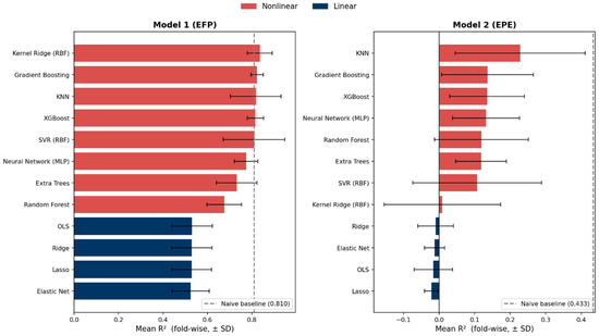
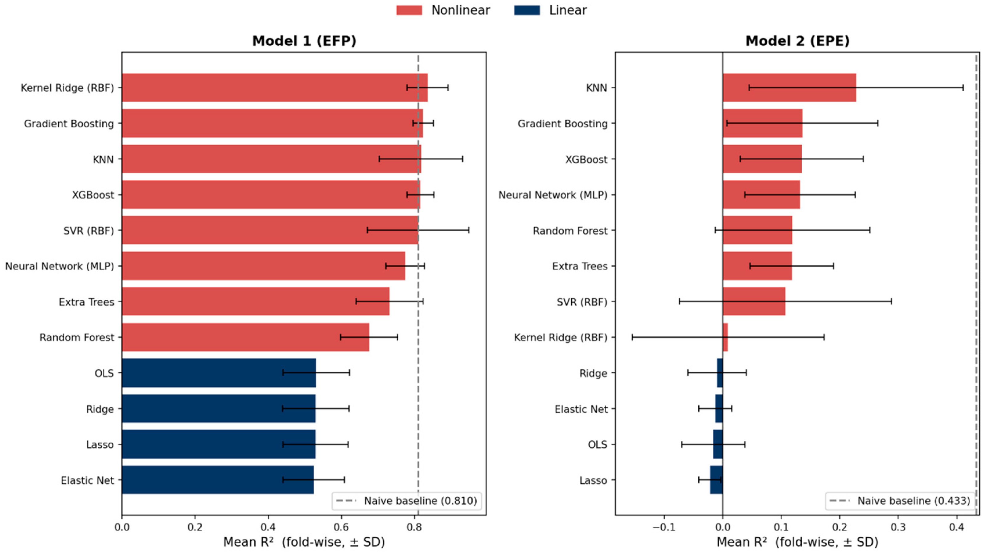
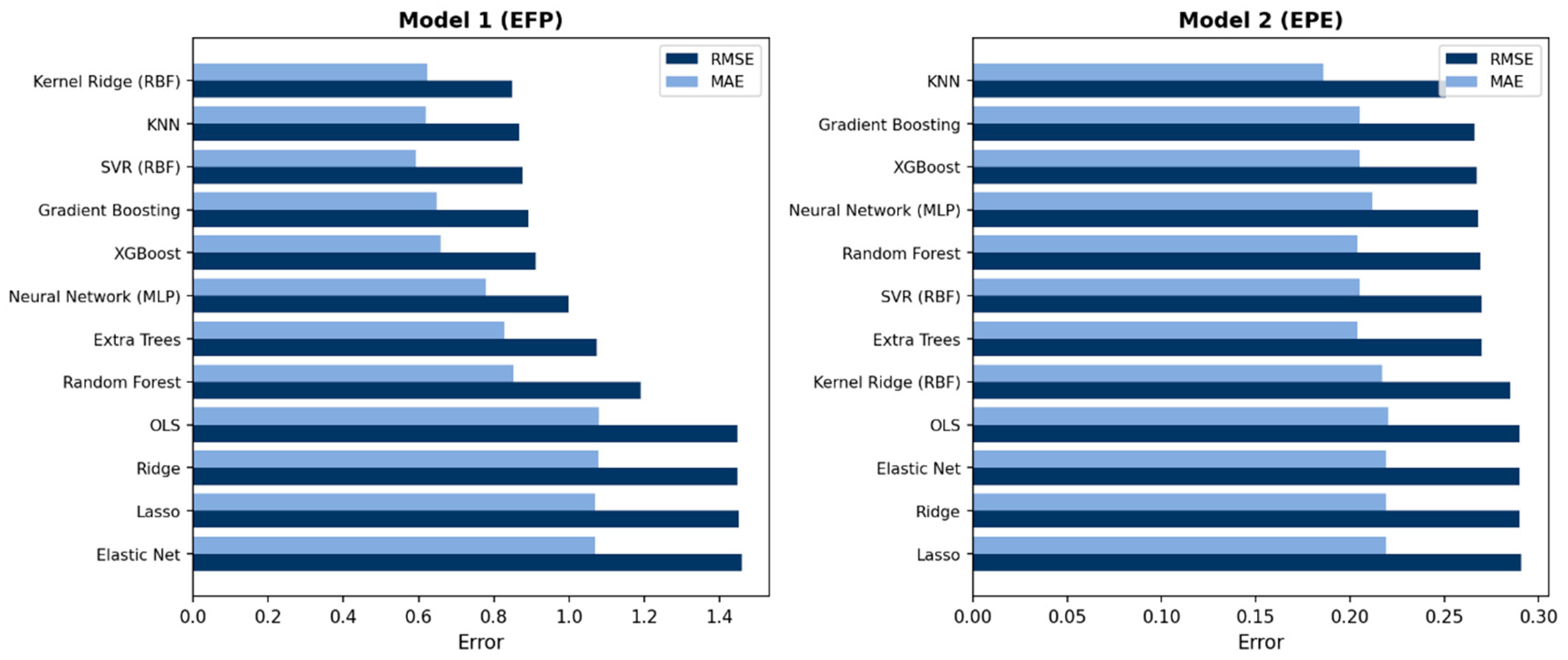
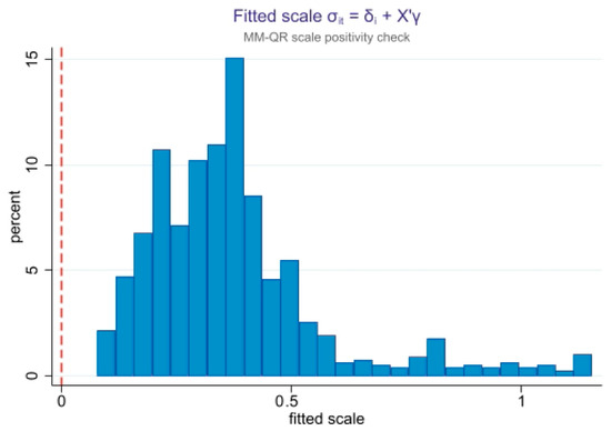
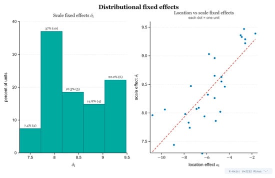
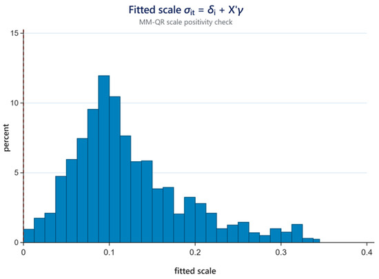
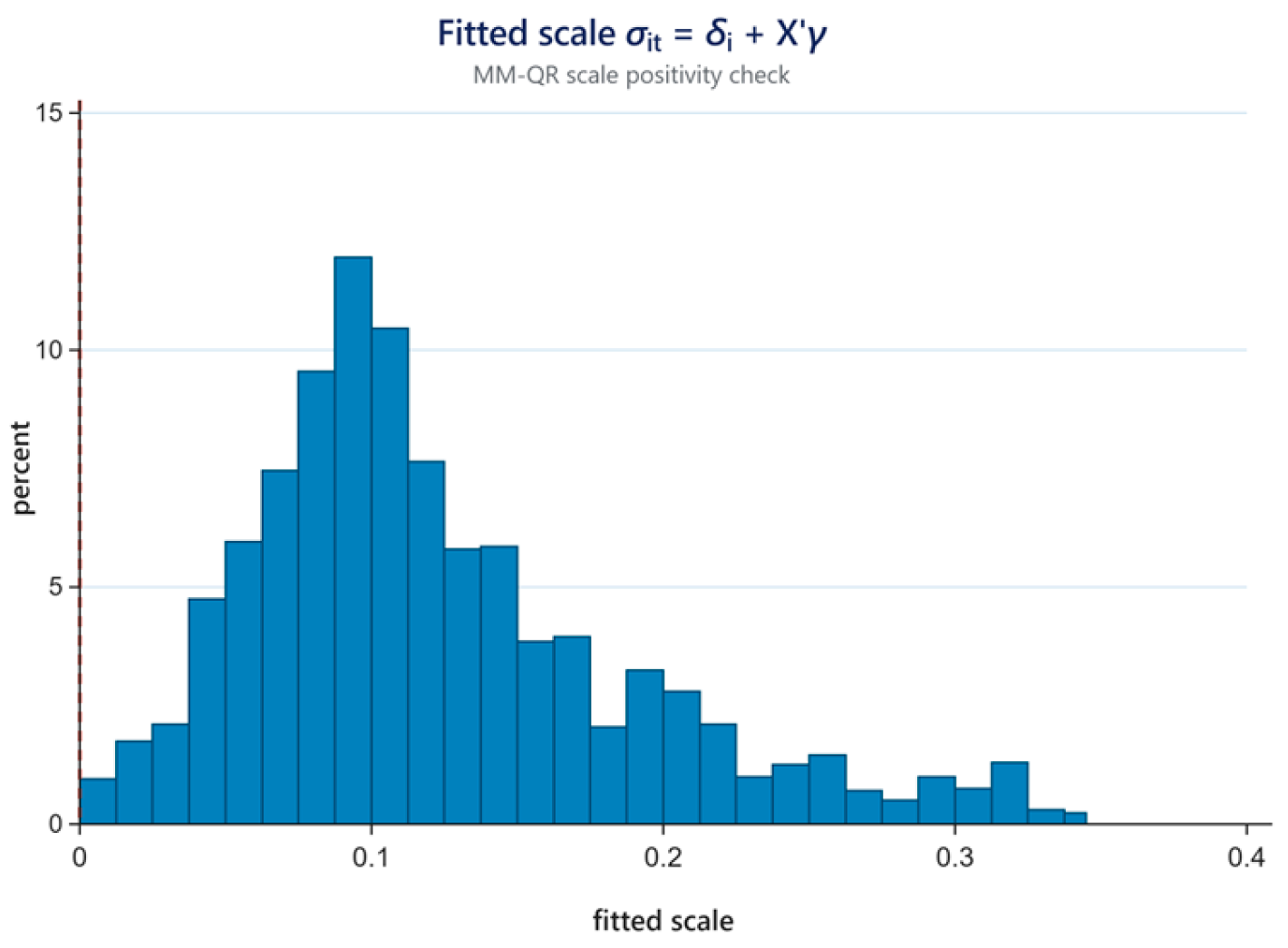
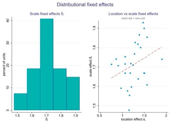
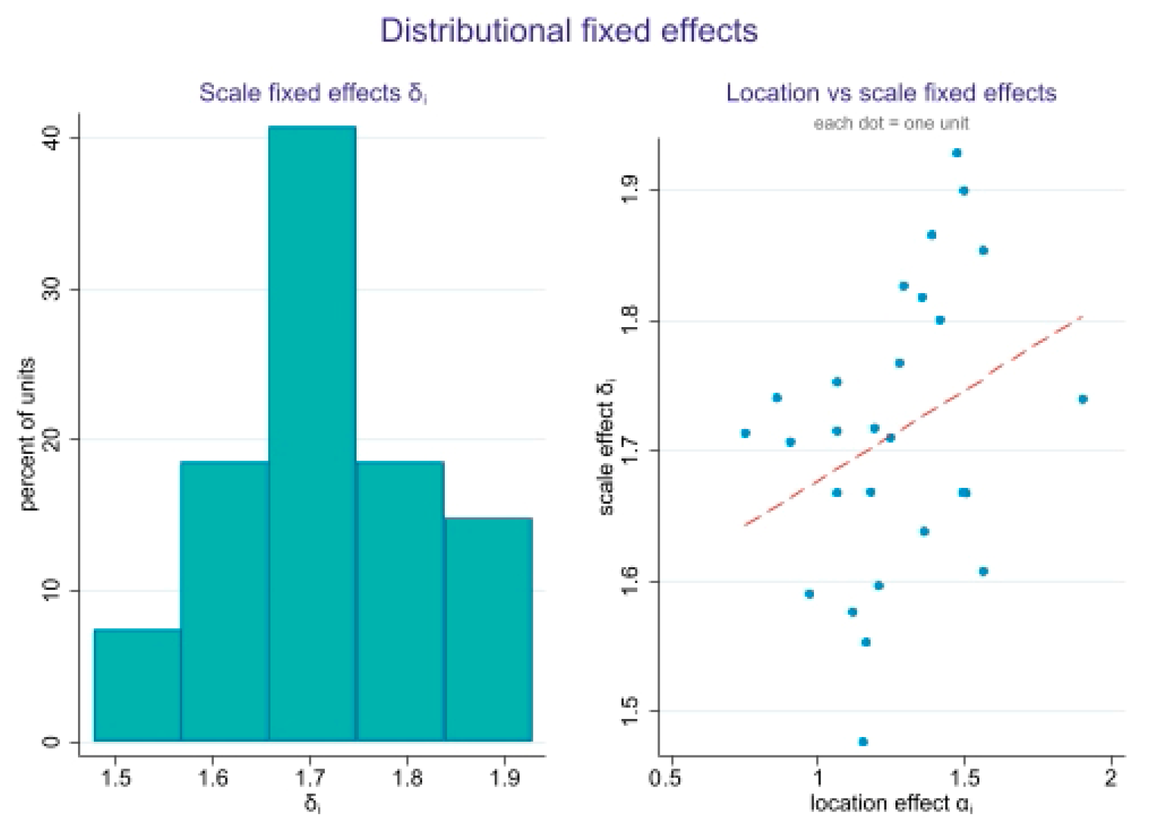

Disclaimer/Publisher’s Note: The statements, opinions and data contained in all publications are solely those of the individual author(s) and contributor(s) and not of MDPI and/or the editor(s). MDPI and/or the editor(s) disclaim responsibility for any injury to people or property resulting from any ideas, methods, instructions or products referred to in the content. |
© 2026 by the authors. Licensee MDPI, Basel, Switzerland. This article is an open access article distributed under the terms and conditions of the Creative Commons Attribution (CC BY) license.