Medium and Short-Term Wind Power Forecasting Using LCNN-Mamba Model Based on Quadratic Decomposition

Abstract

Accurate wind power forecasting is essential for advancing sustainable wind energy utilization, stabilizing new energy power systems, and facilitating the low-carbon and sustainable development of the power industry. Aiming to address the challenges of strong non-stationarity, significant multiscale fluctuations, and the difficulty in jointly modeling local dynamics and long-term dependencies in wind power time series, this study proposes a short-to-medium-term wind power forecasting method based on multiscale decomposition and local-global cooperative modeling. First, Seasonal Trend Decomposition (STL) is employed to extract the trend and seasonal components from the raw time series. The residual series is then subjected to Adaptive Noise-Complemented Empirical Mode Decomposition (CEEMDAN) to reveal the underlying non-stationary characteristics. Based on the dominant frequency characteristics, the decomposed components are reconstructed into high, medium, and low-frequency series, which, together with the trend and seasonal components, form a multidimensional set of input features. Second, to accommodate the time-series characteristics of the multiscale components, we designed an LCNN-Mamba forecasting framework that integrates a Local Convolutional Neural Network (LocalCNN) with a state-space model. The LocalCNN is used to model local and multiscale dynamic features, while the multi-layer Mamba state-space module efficiently captures long-term time-series dependencies, thereby achieving a synergistic enhancement of both local sensitivity and global modeling capabilities. The proposed model was validated using actual operational data from wind farms at two different locations. Experimental results show that the proposed approach outperforms traditional forecasting methods in terms of forecasting accuracy, providing a reliable technical reference for wind power grid-connected operation, power dispatching optimization, and the large-scale and high-quality sustainable development of wind energy resources.

1. Introduction

Against the backdrop of the continuous advancement of the carbon peaking and carbon neutrality strategy, wind energy stands as a core pillar of China’s clean and renewable energy system. Large-scale development and high-efficiency utilization of wind power play a critical role in promoting energy structure transformation and low-carbon operation of power systems [1,2,3]. Large-scale onshore wind bases are mostly transmitted via hybrid cascaded HVDC systems, whose power regulation and fault ride-through strategies will exacerbate wind power volatility and non-stationarity. Accurate wind power prediction is essential to optimize HVDC control schemes and suppress grid oscillation risks, as reported in the study by Liu et al. [4]. Restricted by the inherent randomness, volatility and intermittency of wind resources, wind power generation exhibits strong uncertainty. The large-scale grid connection of wind farms inevitably threatens the secure and stable operation of power grids and interferes with power dispatching decisions, which further restricts the wind power accommodation capacity of power systems [5,6]. Accordingly, high-precision wind power forecasting technology, especially advanced modeling approaches suitable for long time-series analysis and multi-scale feature mining, has become an essential technical guarantee for ensuring grid security, assisting HVDC safe operation and realizing the efficient consumption of wind power [7].

In accordance with time-scale classification criteria, wind power forecasting is divided into ultra-short-term, short-term, medium-and-long-term and long-term modes, which correspond to multiple application scenarios including wind turbine regulation, real-time power dispatching, electricity market trading and power system planning [8]. With the rapid development of data-driven technologies, artificial intelligence algorithms have gradually become the mainstream research direction in wind power forecasting owing to their powerful nonlinear fitting ability. Early research mainly adopted recurrent neural networks (RNNs) [9] and their optimized variants, such as long short-term memory (LSTM) [10] and gated recurrent unit (GRU). Cheng et al. constructed an LSTM-based forecasting model to enhance the prediction accuracy of long-term wind power series [11]. Bi-directional LSTM (BiLSTM) was proposed by Zhang et al. to strengthen the capture capability of sequential correlation characteristics [12]. Zhao et al. developed a CNN-GRU hybrid model, where CNN and GRU were applied to extract spatial and temporal features respectively, so as to optimize the global feature learning performance [13]. Although these models alleviate the long-range gradient vanishing issue through unique gating structures, their inherent sequential operation mode limits the modeling efficiency for ultra-long time-series data.

In the broader field of power time-series forecasting, scholars have also focused on solving two common practical problems of intelligent prediction models: excessive computational costs and dependence on sufficient historical data. Ref. [14] proposed a transfer learning framework for short-term load forecasting, which combines sequence feature extraction and clustering to simplify similarity evaluation, and optimizes the fine-tuning process to reduce computational overhead by more than 92% while ensuring prediction accuracy. Aiming at the dilemma of insufficient training samples in distribution network forecasting tasks, Ref. [15] put forward a multi-task small-sample learning method. It clusters load sequences based on similarity metrics to realize effective knowledge transfer and adopts ensemble learning strategies to suppress overfitting under small-sample conditions. These studies provide valuable references for optimizing the training efficiency and generalization ability of time-series prediction models in power systems.

Recently, Transformer architectures have achieved remarkable prediction performance in wind power forecasting and other time-series tasks [16,17,18], benefited from the self-attention mechanism for global dependency capturing. Yan et al. introduced Transformer into wind power prediction, and the comparative results revealed its superiority over conventional CNN and LSTM models [19]. Nevertheless, the quadratic computational complexity of self-attention leads to a sharp increase in computational overhead and memory consumption with the growth of sequence length, severely restricting its applicability to long-term forecasting tasks. To solve this bottleneck, Zhou et al. proposed the Informer model, which effectively improved computational efficiency via sparse attention and generative decoder design [20]. In addition, state space models (SSMs) have emerged as a novel solution for time-series forecasting. Rangapuram et al. adopted SSMs for time-series prediction, yet the model suffered from limited learning performance due to weak feature recognition, insufficient filtering capacity and single distance-dependent dependency constraints [21]. As an advanced SSM variant, the Mamba model proposed by Gu et al. breaks through the inherent defects of Transformer. It realizes dynamic adaptive attention via selective state space conversion and reduces computational complexity through parallel computing design [22]. However, Mamba exhibits poor adaptability to abrupt fluctuations of non-stationary data and insufficient sensitivity to short-term abnormal features. It remains challenging to balance local dynamic variation and global evolution trends in wind power time-series analysis, especially for wind sequences with intensified non-stationarity caused by HVDC power adjustment.

Signal decomposition technology is widely adopted to eliminate the non-stationarity of original wind power data [23,24,25]. Current research mostly relies on single decomposition algorithms, such as empirical mode decomposition (EMD) [26], ensemble empirical mode decomposition (EEMD) [27] and variational mode decomposition (VMD) [28]. These methods can reduce the difficulty of nonlinear modeling, but still have obvious defects in suppressing modal aliasing and mining multi-scale comprehensive features: single decomposition cannot separate trend and seasonal components in advance, leaving residual trend interference that fails to fully eliminate data non-stationarity. To address such deficiencies, multi-stage and hybrid decomposition strategies have been widely explored. Xiang et al. adopted the VMD-CEEMDAN secondary decomposition framework to fully mine residual fluctuation information [29]. Wang et al. proposed a combined CCVMD-STL decomposition method to integrate data denoising and multi-scale feature extraction [30]. Secondary decomposition can decompose non-stationary original sequences into multiple stable sub-sequences, thus improving prediction accuracy and model interpretability. Most existing hybrid decomposition-deep learning schemes simply combine two-stage decomposition with LSTM, CNN or Transformer. Such frameworks either fail to balance local multi-scale feature extraction and long-sequence global modeling, or incur excessive computational costs, making them unsuitable for online prediction in large-scale HVDC-connected wind farms. Lacking unified decomposition rules and collaborative optimization between decomposition and prediction modules, existing methods struggle to simultaneously address wind power’s non-stationarity and multi-scale coupling fluctuations [31,32]. Therefore, it is urgent to establish an integrated forecasting framework that balances multi-scale feature representation and high-efficiency long-sequence modeling.

Targeting the above limitations, this study develops a novel wind power forecasting framework combining multi-scale secondary decomposition and local–global collaborative modeling. The core innovation lies in the complementary coupling of STL-CEEMDAN secondary decomposition and the Mamba model, which serves as the optimal solution to tackle the non-stationarity and multi-scale fluctuations of wind power time series under the HVDC wind power delivery background. STL is first adopted to separate trend and seasonal components so as to eliminate long-term drift interference, and the residual fluctuation sequence is further processed by CEEMDAN to suppress modal aliasing and realize hierarchical decoupling of multi-scale features. Benefiting from its linear computational complexity, Mamba efficiently mines long-range temporal dependencies of each decomposed stable subsequence, which well remedies the defect that the original Mamba model fails to fit abrupt fluctuations of raw non-stationary wind data. On this basis, a customized LocalCNN module is introduced to capture local short-term abnormal dynamic features, forming a local–global collaborative prediction structure that gives full play to the respective strengths of local feature extraction and global long-sequence modeling. In the preprocessing stage, all decomposed subsequences are reconstructed into high-frequency, medium-frequency and low-frequency components according to dominant frequency characteristics, which are fused with trend and seasonal items to construct multi-dimensional input features for comprehensively describing wind power fluctuation rules. The LocalCNN-Mamba hybrid model is then used to implement high-efficiency time-series prediction. Experimental results verify that the proposed framework achieves outstanding performance in prediction accuracy and numerical robustness. This research can offer reliable technical references for short-term wind power forecasting, refined power grid dispatching as well as the fault ride-through optimization of HVDC wind transmission systems.

2. Methodology

2.1. Data Processing

2.1.1. Data Preprocessing and Partitioning

This paper uses historical operational data from a wind farm in Inner Mongolia as a case study. From the wind farm’s data repository, we selected complete observation data covering the period from 1 January 2021 to 12 March 2023, collecting a total of 76,968 valid observation points as the experimental sample, with a data sampling interval set at 15 min.

In wind power forecasting tasks, raw monitoring data is prone to being affected by equipment malfunctions and environmental disturbances, often containing missing values and outliers. Directly using such data for modeling can distort the statistical characteristics of the time series and reduce the reliability of forecasting results [33,34,35]. Therefore, this paper first conducts data cleaning and repair. Based on the physical constraints of wind turbine operation, a reasonable range of 0–50 MW is defined for the power data; samples exceeding this range are identified as outliers and repaired by linear interpolation. This approach maintains the continuity of the time series while avoiding the introduction of additional assumptions. After processing, the completeness and physical consistency of the data are significantly improved, laying a reliable foundation for subsequent modeling.

To ensure the objectivity of model evaluation, the data is divided into training, validation, and test sets in chronological order at a ratio of 7:1:2. This division strategy prevents information leakage and ensures the validity of the generalization ability assessment. In addition, to address the problem of inconsistent variable units, the Min–Max normalization method is adopted to map the data to the interval [0, 1], thereby improving the numerical stability and convergence efficiency of model training. The calculation formula is presented as follows. It should be noted that the normalization parameters are derived exclusively from the statistics of the training set and are uniformly applied to both the validation and test sets.

$$x^{\prime }={\displaystyle \frac{x-x_{\min }}{x_{\max }-x_{\min }}}$$

(1)

2.1.2. Feature Engineering Analysis

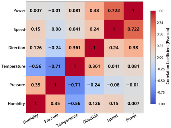
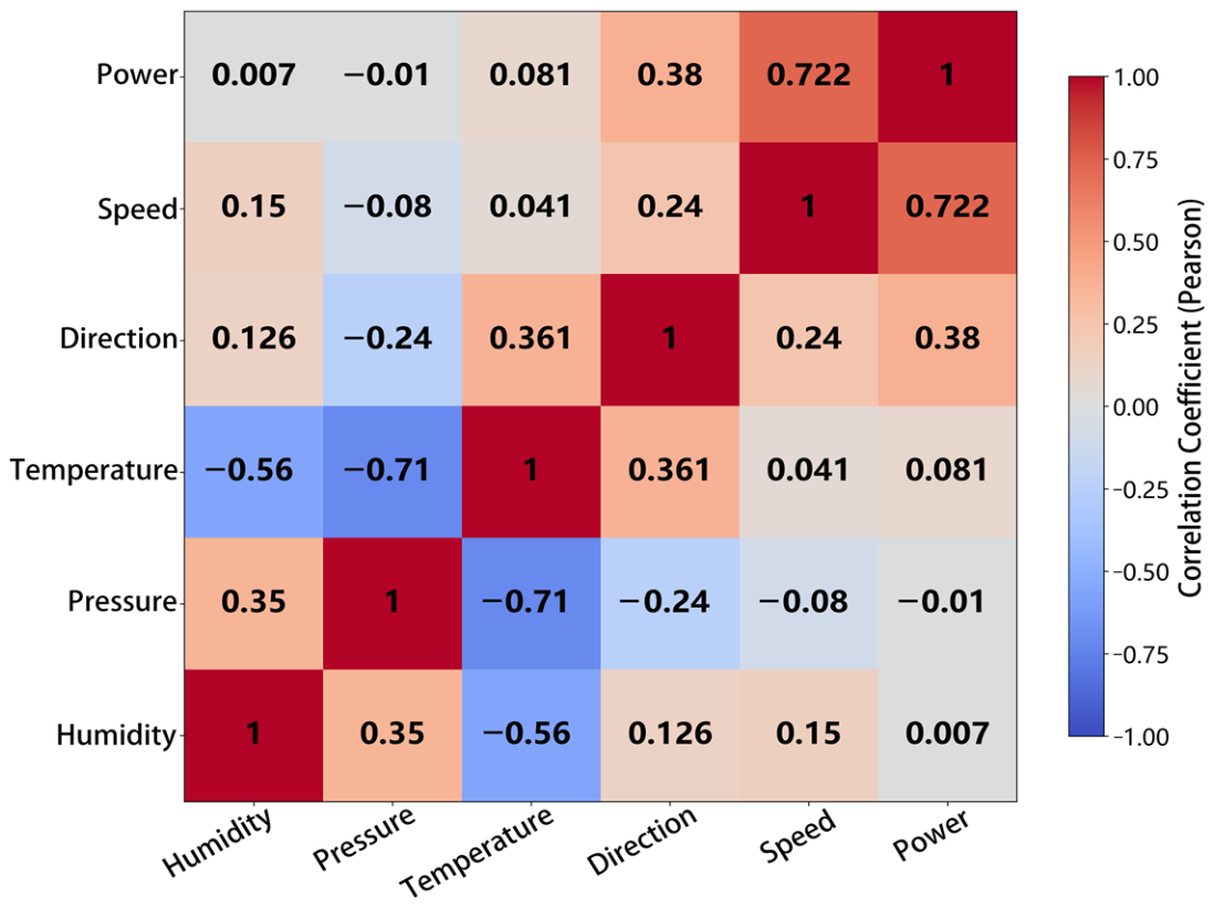
Feature engineering is a critical step in enhancing model performance and generalization ability. By filtering and optimizing original variables, we can effectively reduce interference from redundant information, as well as improve the model’s interpretability and computational efficiency. To quantitatively evaluate the relationships between each variable and the target variable, this paper adopts Pearson’s correlation coefficient to conduct correlation analysis on the features [36]. As illustrated in Figure 1, only wind speed and wind direction show a significant correlation with power, while the linear correlations between the remaining variables and the target variable are weak, suggesting their limited overall contribution.

Figure 1. Heatmap of variable correlations.

Furthermore, a certain degree of correlation exists among the features, indicating potential multicollinearity issues. Such issues may introduce redundant information and increase model complexity in multi-feature modeling. Considering both the strength of variable correlations and feature redundancy, and to achieve model simplification and effective information representation, this study ultimately selects wind speed and wind direction as the input features for modeling. The basic statistical characteristics of the wind power, wind speed and wind direction dataset used in this paper are summarized in Table 1. This approach not only ensures the retention of key information but also enhances the model’s stability and interpretability. During the feature input process, wind speed and power are represented by their raw measured values. However, wind direction, as a meteorological feature with periodic circular characteristics, may lead to disordered biases in model training if its raw angular information is directly used. To address this problem, this study employs a dual-variable encoding strategy using sine and cosine functions to realize continuous mapping of wind direction. Specifically, given the raw wind direction angle θ, the wind direction is decomposed into two orthogonal components, denoted as wind(x) and wind(y), which capture its periodicity in a continuous, linearized form. The corresponding mathematical expressions are given as follows:

$$wind(x)=\cos ({\displaystyle \frac{\theta \pi }{180}})$$

(2)

$$wind(y)=\sin ({\displaystyle \frac{\theta \pi }{180}})$$

(3)

Table 1. Statistics for the dataset.

Variable	Sample Size	Max Value	Min Value	Mean Value
Wind Power/MW	76,968	50.00	0.00	26.59
Wind Speed/(m·s−1)		27.00	0.60	9.42
Wind Direction/°		356.00	4.00	236.93

2.1.3. Secondary Decomposition

Wind power time series are influenced by both meteorological conditions and wind turbine operating states, typically exhibiting pronounced non-stationarity and multi-scale fluctuations. This makes it challenging to effectively capture their underlying patterns through direct modeling. Traditional single-decomposition methods often struggle to balance trend extraction, periodicity characterization, and the separation of high-frequency disturbances, frequently resulting in issues such as modal aliasing. To address this limitation, this paper proposes an STL–CEEMDAN two-stage decomposition framework: first, STL is applied to decompose the original time series, extracting trend and seasonal components to reduce the complexity of the series; subsequently, CEEMDAN is applied to the residual term for adaptive decomposition, thereby enabling more refined characterization of multi-scale features.

STL is a time series decomposition method based on locally weighted regression, which decomposes the original series into three components: trend, seasonal, and residual. The STL algorithm comprises an inner loop and an outer loop: the inner loop iteratively generates the trend, seasonal, and residual components, while the outer loop performs robust weight calculations to mitigate the impact of outliers [37,38]. the corresponding mathematical expressions are as follows:

$$y(t)=T(t)+S(t)+R(t)$$

(4)

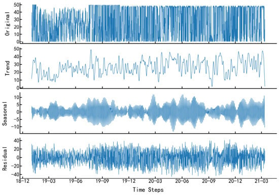
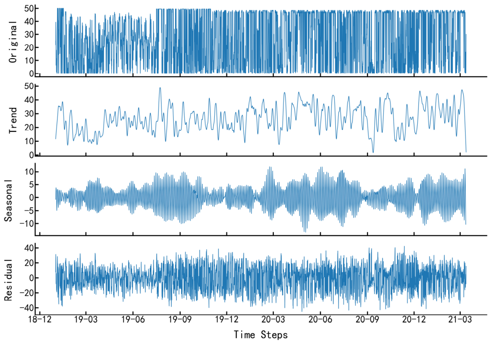
where $y(t)$ is the original wind power time series, $T(t)$ is the trend component, $S(t)$ is the seasonal component, and $R(t)$ indicates the residual component containing high-frequency fluctuations and random disturbances. STL performs iterative smoothing on the time series using local regression (Loess), which ensures the stability of decomposition while exhibiting strong robustness against outliers, making it suitable for wind power data with distinct periodic characteristics. Combined with the decomposition results presented in Figure 2, it can be observed that STL demonstrates excellent separation capability in the preprocessing stage: its trend component smoothly reflects the long-term evolution patterns, the seasonal component exhibits stable periodic oscillations, and the residual component concentrates high-frequency random disturbances, with clear component separation and minimal mutual interference. Building on this, further decomposing the structurally complex residual component using CEEMDAN can deeply reveal its nonlinear and multi-scale information.

Figure 2. STL Exploded view.

By adding adaptive white noise to the original signal and performing multiple ensemble decompositions, CEEMDAN effectively alleviates the modal aliasing problem existing in traditional EMD and EEMD. This method decomposes complex signals into several intrinsic modal functions (IMFs) and a residual term [39], which can be mathematically expressed as follows:

$$R(t)={\displaystyle \sum _{k=1}^{K}IM{F}_k(t)+r(t)}$$

(5)

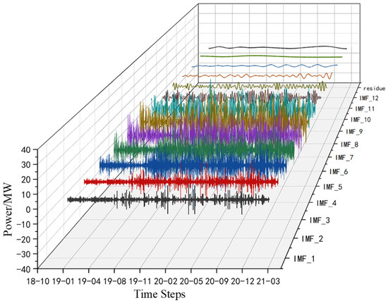
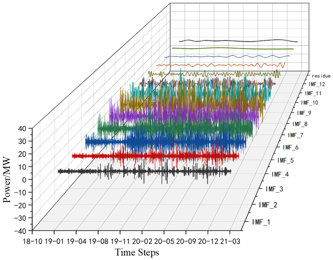
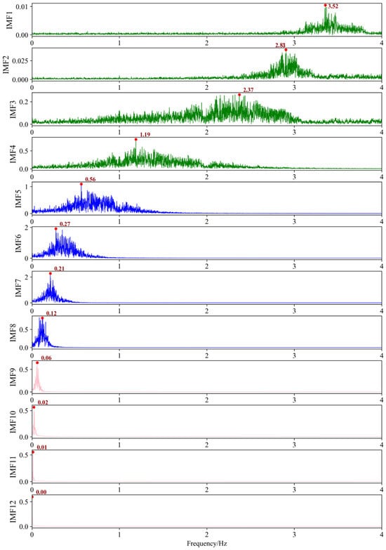
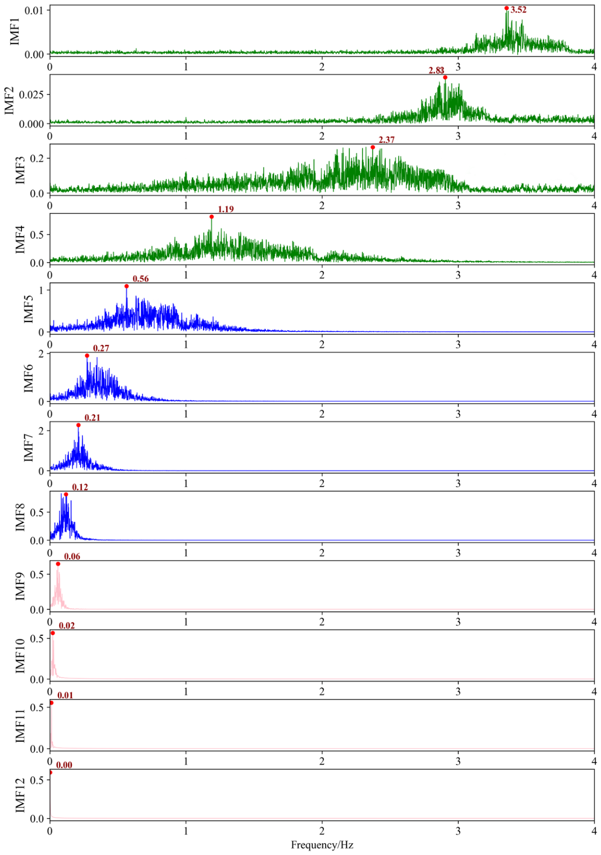
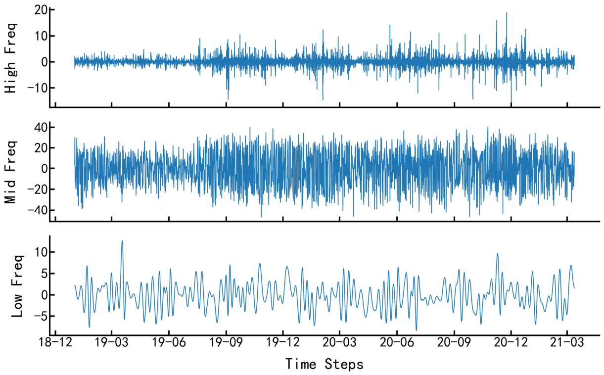
where $IM{F}_k(t)$ is the oscillatory components at different time scales; $r(t)$ is the final residual term. The CEEMDAN decomposition results of the STL residual term are presented in Figure 3. To avoid feature redundancy and increased model complexity induced by inputting all IMF components, this paper further sorts and reconstructs the IMF components based on their dominant frequency characteristics. As illustrated by the Hilbert spectrum of each decomposed IMF component in Figure 4, quantitative frequency thresholds reserved to two decimal places are defined to categorize the components, and the red dots plotted in each panel represent the dominant frequency of every decomposed IMF component: IMFs with dominant frequencies ranging from 1 Hz to 4 Hz are defined as high-frequency components, those with dominant frequencies between 0.1 Hz and 1 Hz are categorized as medium-frequency components, and components with dominant frequencies below 0.1 Hz are grouped into low-frequency components. Different colors are adopted to visually distinguish these three frequency bands. The components are classified in descending order of their dominant frequencies: high-frequency components are merged into a high-frequency sub-sequence, medium-frequency components into a medium-frequency sub-sequence, and low-frequency components together with the residual term into a low-frequency sub-sequence. This approach reduces the feature dimension while retaining key multi-scale information. The three merged frequency bands are illustrated in Figure 5. Finally, the trend and seasonal components obtained from STL decomposition, combined with the high-frequency, medium-frequency, and low-frequency sequences reconstructed by CEEMDAN, form a five-dimensional input feature set. These features are fed into the subsequent forecasting model for joint modeling, providing multi-scale information support for local-global collaborative forecasting.

Figure 3. CEEMDAN Exploded view.

Figure 4. Hilbert Spectrum of CEEMDAN Decomposed IMF Components.

Figure 5. Merged tri-band image.

2.1.4. Comparison of Different Decomposition Methods

To quantify the role of quadratic decomposition in wind power sequence processing, this paper validates its advantages by comparing various signal decomposition methods, including CEEMDAN, EWT, FIF, RLMD, and STL, and constructs four types of quadratic decomposition methods: STL-CEEMDAN, STL-EWT, STL-FIF, and STL-RLMD. Specifically, CEEMDAN suppresses modal aliasing through noise-assisted and integral decomposition; EWT constructs filters based on adaptive spectral segmentation [40]; FIF achieves signal separation via iterative filtering [41]; RLMD performs modulation decomposition based on local envelope means [42]; and STL decomposes time series into trend, seasonal, and residual components using locally weighted regression, thereby providing structural prior information for subsequent fine-grained decomposition.

To quantitatively evaluate the performance of different decomposition methods, four evaluation metrics were selected: the maximum adjacent IMF correlation coefficient (MAC), median baseline drift ratio (MBWR), number of IMFs (N), and total computation time (T). Among these metrics, MAC quantifies the independence between modes, while MBWR reflects frequency purity; smaller values of both indicators indicate better decomposition performance. N represents the level of decomposition detail, and T measures algorithmic efficiency. Experimental results show that among single decomposition methods, CEEMDAN performs superiorly in terms of modal independence and frequency purity, whereas EWT and RLMD exhibit significant limitations in modal independence and frequency separation. FIF achieves balanced overall performance but has limited effectiveness in reducing inter-modal correlation.

In contrast, the quadratic decomposition methods incorporating STL exhibited a significant overall improvement in performance. Among these, STL-CEEMDAN achieved the optimal results in both key metrics—modal independence and frequency purity—outperforming other methods significantly. It effectively suppresses modal aliasing and improves frequency separation accuracy, yielding 12 IMFs and demonstrating high decomposition resolution. Although other quadratic decomposition methods show certain improvements, they still have obvious shortcomings. For instance, STL-FIF has an MBWR as high as 1.13, indicating severe baseline drift in its decomposition results. Although STL-CEEMDAN requires relatively more computation time, this cost is acceptable given its significant advantages in decomposition quality. The evaluation results of all decomposition models are presented in Table 2.

Table 2. Performance metrics of different decomposition models.

Decomposition Model	MAC	MBWR	N	T/s
CEEMDAN	0.35	0.44	16	445.32 s
EWT	0.27	0.23	6	1.54 s
FIF	0.36	0.31	10	4.09 s
RLMD	0.32	0.05	8	1.61 s
STL-CEEMDAN	0.17	0.01	12	538.59 s
STL-EWT	0.62	0.49	6	81.07 s
STL-FIF	0.50	0.65	10	86.42 s
STL-RLMD	0.39	1.13	9	81.30 s

To further analyze the role of the STL in the secondary decomposition, the results of the standalone STL decomposition were evaluated. The results show that the standard deviation of the first-order difference in the trend component $SD(\Delta T)=0.04$, indicating that trend extraction is smooth and stable; the correlation coefficient between the original sequence and the trend component $Corr(X,T)=0.89$, indicating that the trend component effectively characterizes the primary variations in the original sequence; the peak of the seasonal component’s autocorrelation function $AC{F}_{peak}(S)=0.99$, indicating that the periodic structure has been fully extracted; and the correlation coefficient between the trend and seasonal components $\left|Corr(T,S)\right|=0.001$, indicating that the two have achieved good decoupling. The results demonstrate that STL can decompose the original sequence into components with clear structures that are mutually independent, significantly reducing signal complexity.

From a mechanistic perspective, after STL removes the trend and periodic components, the residual signal consists primarily of random fluctuations and mid-to-high-frequency details, with a more dispersed frequency distribution. Building on this, CEEMDAN adaptively separates multiscale oscillatory components through noise-assisted and integral decomposition, avoiding modal aliasing and yielding more independent narrowband IMF components, resulting in STL-CEEMDAN performing optimally on core metrics. EWT relies on clear spectral boundaries and is prone to segmentation errors when processing structurally complex residual signals; FIF is more suitable for stationary signals and has limited ability to separate random fluctuations; RLMD is biased toward low-frequency modulated signals and is prone to aliasing when processing high-frequency random components. Therefore, the performance of the aforementioned methods in the second-order decomposition framework is inferior to that of STL-CEEMDAN.

In summary, STL plays a crucial preprocessing role in the second-order decomposition, while CEEMDAN offers significant advantages in handling complex non-stationary residual signals. The combination of the two effectively improves the decomposition quality of wind power time series, providing more stable and physically meaningful input features for subsequent neural network models. Moreover, this two-stage hybrid decomposition framework realizes hierarchical screening of signal components at the preprocessing stage, which effectively avoids massive repetitive and redundant comparative experiments in the subsequent prediction chapter and streamlines the overall experimental layout of the manuscript. Meanwhile, it establishes a solid theoretical basis for the rationality of adopting multi-scale secondary decomposition rather than single decomposition in wind power forecasting tasks.

2.2. LCNN-Mamba Prediction Model

2.2.1. LCNN Module

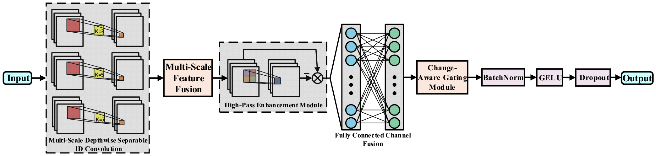
Time series of wind power output often exhibit local dynamic behaviors (e.g., sudden changes, gradual increases, and high-frequency disturbances) on short time scales, which are the primary sources of prediction errors. Affected by HVDC power regulation and random wind fluctuations, such local abrupt and high-frequency features are easily submerged in global long-term trend information, leading the Mamba model to ignore local transient mutation details and degrade prediction accuracy. Therefore, the core design principle of the proposed Local Convolutional Neural Network (LCNN) module is to make up for the inherent deficiency of state-space models in local fine-grained feature extraction. From the perspective of physical engineering significance, it aims to effectively capture wind power ramp events, short-term power fluctuations and abnormal transient disturbances in actual power grid operation, and achieve adaptive enhancement of local sensitive features under complex operating conditions, so as to reduce the prediction error caused by neglect of local dynamic characteristics. This module serves as an embedded local feature enhancement unit that collaborates with subsequent state-space models, as illustrated in Figure 6. The LCNN does not directly undertake the forecasting task; instead, by applying structured local enhancement to the input sequence, it highlights key time-varying features while preserving the original trend information, thereby providing a more discriminative input representation for long-sequence modeling.

Figure 6. Schematic diagram of the LCNN module.

The LCNN module is built on the input time-series feature $X\in R^{B\times L\times C}$, where B, L, and C denote the batch size, sequence length, and number of channels, respectively. Its overall pipeline follows normalization, multi-scale local modeling, high-pass enhancement, channel reorganization, change-aware gating, and residual fusion. First, RMSNorm is applied to the input feature $\tilde{X}$ to alleviate dimensional discrepancies across components. This normalization operation eliminates the magnitude difference between decomposed subsequences with different fluctuation intensities and lays a unified data foundation for subsequent multi-scale local feature extraction. The depthwise separable 1D convolution operator $DWCon{v}_k(\cdot )$ with kernel lengths $k\in (3,5,7)$ is then used to extract local dynamic features at different temporal windows, yielding the local convolution output $H_k$ at the k-th scale. These multi-scale features are averaged to form a unified local response representation H, as formulated below:

$$H_k=DWCon{v}_k(\tilde{X})$$

(6)

$$H={\displaystyle \frac{1}{3}}{\displaystyle \sum _k{H}_k}$$

(7)

Next, a high-pass enhancement operation is constructed using the temporal sliding average pooling operator $AvgPool(\cdot )$, producing the high-pass enhanced local feature $H_{hp}$ to highlight rapid variations in the sequence. In physical essence, this operation filters out slow-varying low-frequency trend components and retains transient high-frequency fluctuation details closely related to wind power prediction errors. The enhanced feature is then processed via temporal-wise channel linear transformation $Con{v}_{1\times 1}(\cdot )$, batch normalization (BN), GELU activation $\varphi (\cdot )$, and dropout regularization $Dropout(\cdot )$ to reorganize cross-channel features, improve representational capacity, and mitigate overfitting, resulting in the local enhanced feature Z. The corresponding formulations are given as

$$H_{hp}=H-AvgPool(H)$$

(8)

$$Z=Dropout(\varphi (BN(Con{v}_{1\times 1}(H_{hp}))))$$

(9)

Meanwhile, a change-aware gating mechanism is constructed based on the absolute value of the first-order difference in the input sequence at time step t, defined as $\Delta X_t$. This parameter-adaptive gating mechanism dynamically adjusts the feature enhancement weight according to the real-time fluctuation intensity of wind power data, avoiding over-enhancement of stable flat segments and insufficient feature extraction of abrupt mutation segments. The sigmoid-activated convolution layer generates the gating weight matrix $G\in (0,1)$ to modulate the intensity of local enhancement. Finally, residual fusion is performed with a scaling coefficient $\alpha$ to control the enhancement magnitude, combining the gated local feature with the original input to achieve a balance between local enhancement and global stability, and producing the LCNN output feature $X^{\prime }$. The mathematical expressions are:

$$\Delta X_t=\left|X_t-X_{t-1}\right|$$

(10)

$$G=\sigma (Con{v}_{1\times 1}(\Delta X))$$

(11)

$$X^{\prime }=X+\alpha (Z\odot G)$$

(12)

2.2.2. Mamba Module

Mamba is an efficient deep learning architecture tailored for long-sequence modeling [43]. Built on state-space model (SSM) theory, it incorporates an input-driven selection mechanism to enhance its expressive power. By integrating linear mapping, gating control, and selective state-space modeling, Mamba can adaptively regulate information flow, emphasize key contextual information, and suppress redundant content. Computationally, Mamba achieves computational efficiency that scales linearly with sequence length through structural reorganization. Combined with parallelization strategies to accelerate inference, it offers both efficiency and performance advantages over traditional SSMs and attention-based models in long-sequence modeling tasks.

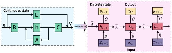
State-space models describe the evolution of a sequence via hidden state variables, transforming input $x(t)\in R^D$ into a representation of hidden state $h(t)\in R^N$ that is recursively updated over time. At its core, the model employs state transitions and input mappings to compress and propagate historical information, a process described by the following linear ordinary differential equation:

$$\dot{h}(t)=Ah(t)+Bx(t)$$

(13)

$$y(t)=Ch(t)$$

(14)

where $y(t)\in R^N$ is the output sequence, and $A\in R^{N\times N}$ and $B,C\in R^{N\times D}$ are learnable matrices. To adapt to deep learning, the SSM is treated as a continuous-time model and discretized using a zero-order holder (ZOH). Therefore, the continuous-time parameters A and B are converted into discrete counterparts $\overline{A}$ and $\overline{B}$ by adopting the time-scale parameter Δ The discretized SSM can be expressed as:

$$h_t=\overline{A}{h}_{t-1}+\overline{B}{x}_t$$

(15)

$$y_t=C{h}_t$$

(16)

$$\overline{A}=\exp (\Delta A)$$

(17)

$$\overline{B}={(\Delta A)}^{-1}\cdot (\exp (\Delta A)-I)\cdot \Delta B$$

(18)

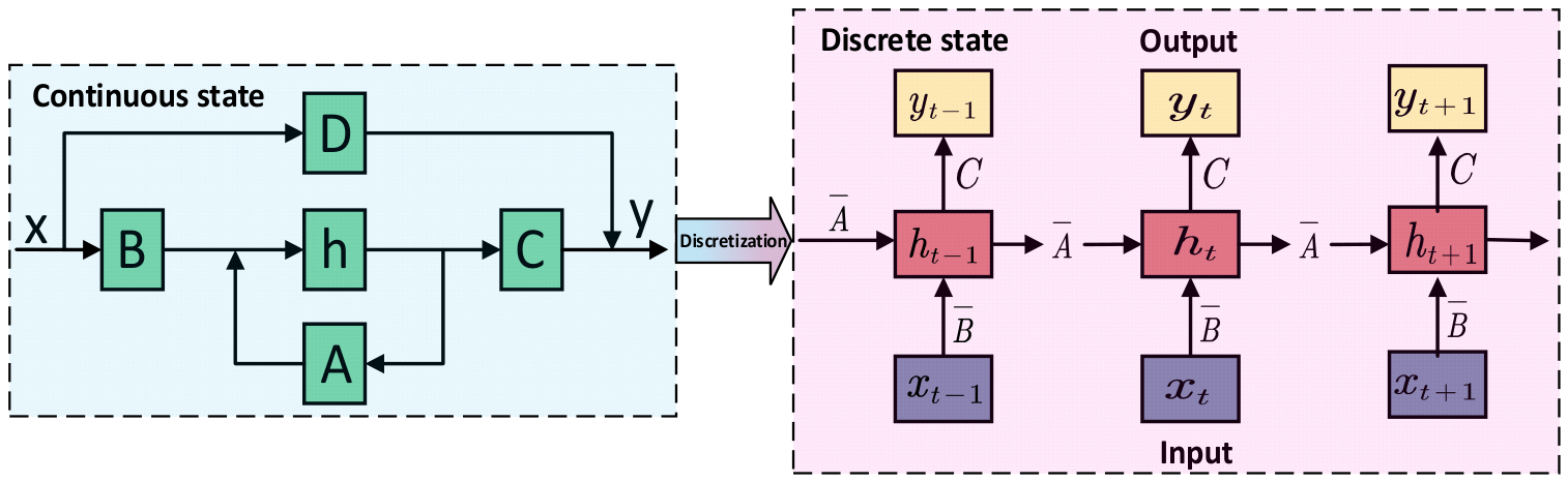
In discrete form, the model can be formulated as a recursive update process, which enables long-sequence data processing with linear computational complexity. From a convolutional perspective, the SSM is equivalent to deploying a structured global convolutional kernel on the input sequence, thereby empowering the model to capture long-range dependencies, as demonstrated in Figure 7. Nevertheless, conventional SSMs adopt fixed parameter settings that fail to adjust dynamically with input variations, which restricts their capacity to extract key information under complex operating conditions.

Figure 7. Block diagram of the SSM in continuous and discrete states.

To tackle this limitation, Mamba integrates a selective modeling mechanism into the SSM framework. It parameterizes state transitions, input projections, and time steps as input-dependent functions, realizing dynamic information filtering and adaptive sequence modeling. In the selective state-space modeling paradigm, model parameters are no longer fixed but dynamically generated from the input sequence, which further strengthens the capability to capture long-range dependencies and key feature information. Specifically, the input mapping matrix B, output mapping matrix C, and time step Δ are all defined as functions of the input variable x:

$$B=S_B(x)$$

(19)

$$C=S_C(x)$$

(20)

$$\Delta ={\tau }_{\Delta }(\Delta +S_{\Delta }(x))$$

(21)

where $x\in R^{B\times L\times D}$ is the input sequence, B is the batch size, L indicates the sequence length, and D is the feature dimension. Accordingly, $B,C\in R^{B\times L\times N}$ is adopted to realize mapping from the input space to the state space, while $\Delta \in R^{B\times L\times D}$ serves to regulate the time scale throughout the discretization procedure. In practical implementation, the functions $S_B(\cdot )$ and $S_C(\cdot )$ generally adopt linear mappings to project input features into the N-dimensional state space. By comparison, $S_{\Delta }(\cdot )$ first generates scalars through low-dimensional linear transformation, and then expands these scalars to a dimension consistent with input channels via the broadcasting mechanism, which enables unified modulation across all feature channels. Furthermore, the Softplus function ${\tau }_{\Delta }(\cdot )$ is incorporated for nonlinear transformation to guarantee positive time steps and improve numerical stability.

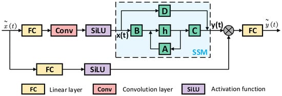
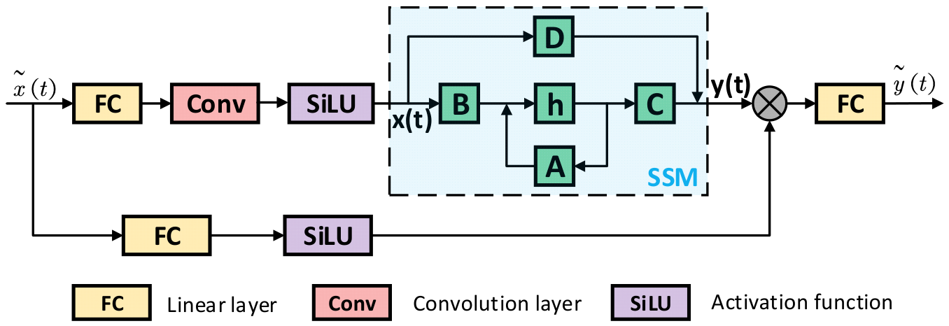
The overall architecture of Mamba consists of repeated Mamba blocks, residual connections, and standard normalization layers. Each Mamba Block follows a core workflow of “feature mapping—local modeling—gated modulation—selective state-space modeling”: the input first undergoes channel mapping via a fully connected layer, extracts local contextual information through convolutional operations, generates gating signals via the SiLU activation function to adaptively modulate feature weights, and finally achieves feature fusion through output mapping and residual connections. This ensures training stability while enhancing the model’s expressive power. The specific structure of the Mamba Block is illustrated in Figure 8. While maintaining linear computational complexity, it integrates local feature extraction with global dependency modeling capabilities, leading to superior performance in long-sequence tasks compared to traditional models.

Figure 8. Mamba Block diagram.

2.2.3. Overall Predictive Model Architecture

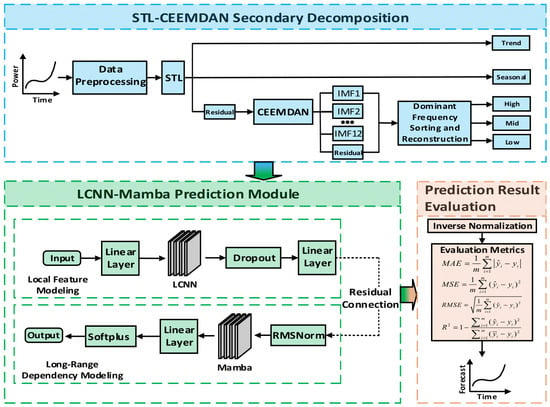
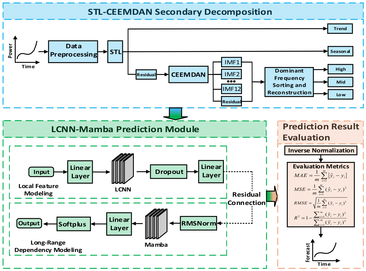
This paper proposes a combined forecasting framework based on STL-CEEMDAN secondary decomposition and LCNN-Mamba. The overall structure of the forecasting model is illustrated in Figure 9. First, after preprocessing the original time series, STL decomposition is applied to decompose the series into trend, seasonal, and residual components; the residual component is further decomposed into multiple intrinsic mode functions (IMFs) and a residual term via CEEMDAN decomposition. Subsequently, based on frequency-domain characteristics, the IMF components are sorted by their dominant frequencies and reconstructed to form high-frequency, medium-frequency, and low-frequency sub-sequences, thereby achieving a multiscale decoupled representation of the original complex non-stationary signal. These decomposition results serve as inputs for the subsequent prediction module, effectively enhancing the model’s capability to capture features across different time scales.

Figure 9. Overall flowchart of the predictive model.

In the prediction phase, a novel LCNN-Mamba hybrid collaborative architecture is custom-built to address the core challenge of balancing local abrupt fluctuations and long-range global trends in multi-scale wind power time series, which represents our core innovative design. First, decomposed input sequences are projected into a unified latent feature space, where the lightweight LocalCNN module with customized convolution kernels extracts fine-grained short-term abnormal dynamic features and greatly enhances the model’s sensitivity to sudden power mutations, effectively remedying the poor capture ability of vanilla Mamba on local short-scale oscillations. The extracted multi-scale local features are then reshaped and normalized, and embedded residual connections are introduced to alleviate feature degradation, smooth gradient propagation and stabilize model training. Next, the optimized Mamba state space model performs deep global modeling on the enriched feature sequences; relying on its linear computational complexity and selective state transition mechanism, it efficiently mines long-distance temporal dependencies and slow-varying global trends, overcoming the quadratic computational bottleneck of Transformer self-attention. Such complementary coupling of LocalCNN’s local feature extraction strengths and Mamba’s efficient long-sequence modeling capacity forms a unique local–global joint prediction paradigm unavailable to single-component models. Finally, nonlinear mapping generates prediction outputs followed by matched reverse reconstruction post-processing, and multiple quantitative evaluation metrics are adopted to comprehensively assess model performance, verifying the effectiveness and strong generalization of the proposed hybrid framework for complex non-stationary time-series forecasting.

3. Experiments and Results

3.1. Preparations

To validate the effectiveness and robustness of the proposed STL-CEEMDAN-LCNN-Mamba hybrid forecasting model in wind power time series forecasting, this paper conducts single-step and multi-step forecasting experiments, considering the non-stationary and highly volatile nature of wind power data. All experiments were performed in a standardized hardware and software environment to ensure the fairness, comparability, and reproducibility of the results. The model was constructed using a mainstream deep learning framework, integrating the STL-CEEMDAN quadratic time series decomposition, LCNN local feature extraction, and Mamba long-sequence modeling modules. Several classical forecasting models were selected as benchmarks for comparative analysis.

Furthermore, in time series forecasting tasks, the selection of model hyperparameters directly affects both the fitting capability and generalization performance. To ensure the rigor and reproducibility of the experiments, this section provides a unified description of the core hyperparameters of the proposed LCNN-Mamba model; the specific configurations are presented in Table 3.

Table 3. Hyperparameters of the LCNN-Mamba model.

Hyperparameters	Value	Hyperparameters	Value
Batch size	64	Deep convolution kernel size	3/5/7
Input sequence length	96	Loss function	SmoothL1Loss
Prediction stride	1	Optimizer	AdamW
Initial learning rate	0.0008	Train/Validation/Test	7/1/2
Weight decay coefficient	0.001	Warmup epochs	16
Number of Mamba residual layers	4	Warmup start factor	0.2
SSM state dimensions	24	Minimum learning rate	1 × 10−5
Feature scaling factor	3	Gradient clipping threshold	1.0
Dropout probability	0.10	High-pass pooling kernel size	9
Number of rounds for early termination	18	Random seed	42, 123, 2024, 666, 999
Maximum number of training iterations	80	Number of independent runs	5

3.2. Evaluation Criteria

A comprehensive quantitative assessment of the proposed model’s performance in ultra-short-term wind power forecasting is conducted in this paper. Four statistical metrics widely used in regression evaluation are selected, namely the Mean Absolute Error (MAE), Mean Squared Error (MSE), Root Mean Squared Error (RMSE), and Coefficient of Determination (R²), to evaluate the model’s predictive performance. The mathematical definitions of these error metrics are as follows:

$$MAE={\displaystyle \frac{1}{m}}{\displaystyle \sum _{i=1}^m\left|{\widehat{y}}_i-y_i\right|}$$

(22)

$$MSE={\displaystyle \frac{1}{m}}{\displaystyle \sum _{i=1}^m{({\widehat{y}}_i-y_i)}^2}$$

(23)

$$RMSE=\sqrt{{\displaystyle \frac{1}{m}}{\displaystyle \sum _{i=1}^m{({\widehat{y}}_i-y_i)}^2}}$$

(24)

$$R^2=1-{\displaystyle \frac{{\displaystyle {\sum }_{i=1}^m{({\widehat{y}}_i-y_i)}^2}}{{\displaystyle {\sum }_{i=1}^m{({\overline{y}}_i-y_i)}^2}}}$$

(25)

where m denotes the total number of samples, $y_i$ and ${\widehat{y}}_i$ represent the i-th observed value and the corresponding predicted value, respectively, and ${\overline{y}}_i$ is the mean of the observed values.

3.3. Model Comparison Experiment

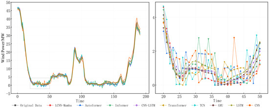
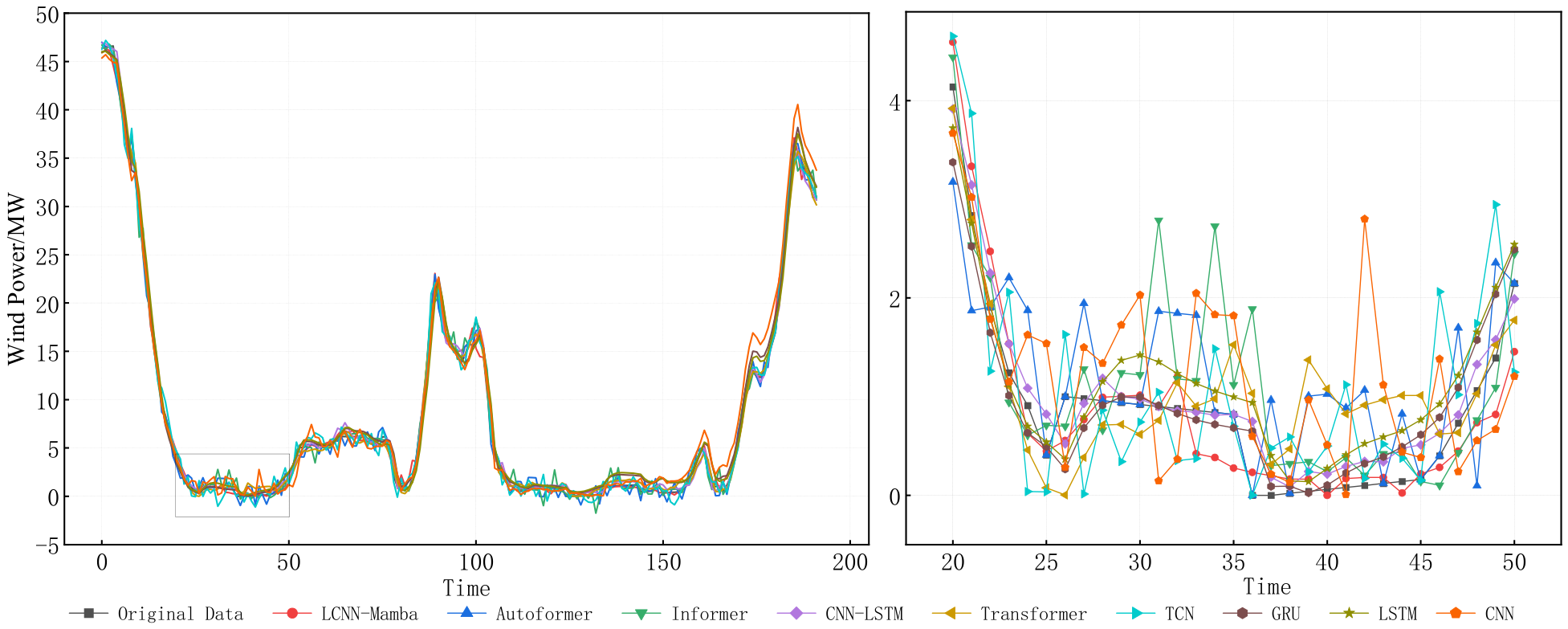
To systematically evaluate model performance on wind power forecasting, this work adopts single-step rolling forecasting with a 15 min time resolution to realize two-day-ahead prediction, where real observed values are used to update the sliding window in each rolling step. Representative samples from the test set are selected for visual comparison. All comparative models use the STL-CEEMDAN secondary decomposition method for data preprocessing. The benchmark methods include recurrent neural networks (RNNs), convolutional neural networks (CNNs), attention-based Transformers and the state-space Mamba model, a high-performance approach for sequence prediction. The proposed LCNN-Mamba model is also included in the comparison. Figure 10 plots the predicted and actual values of all models on the test set, and the enlarged views clearly show the prediction errors under low wind power fluctuations.

Figure 10. Prediction results from different models.

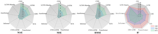
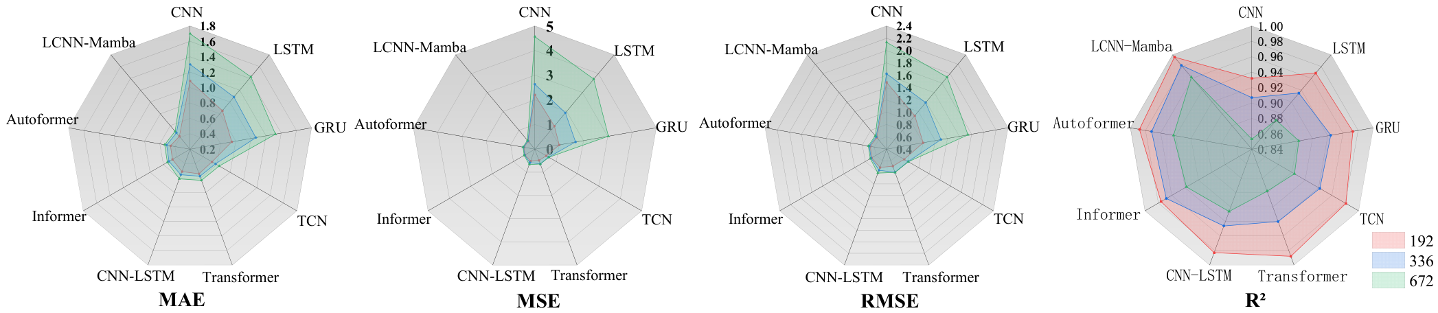
Qualitatively, all comparison models can effectively capture the overall variation patterns and periodic fluctuation trends of wind power time series. As shown in Figure 11, the radar charts of four evaluation metrics intuitively reveal obvious performance gaps among different forecasting frameworks. Significant discrepancies can be observed in their fitting performance and dynamic tracking capabilities during critical intervals featured with violent fluctuations and abrupt changes. Specifically, traditional time series models such as LSTM and GRU are superior in mining temporal dependencies; nevertheless, they generally suffer from response lag and insufficient tracking ability when wind power output changes rapidly and drastically. Restricted by fixed receptive fields, CNN models fail to fully capture short-term abrupt variations and lack dynamic response capacity for extreme fluctuations, which frequently results in peak underestimation, fitting deviations at extreme points and over-smoothing of time series. Benefiting from the global attention mechanism, Transformer achieves relatively satisfying fitting performance yet lacks prediction stability. Within the low-power steady fluctuation range (time steps 20–50), its prediction curve fluctuates sharply with prominent local random errors.

Figure 11. Scatterplot of Performance Metrics for Different Models.

As shown in the local zoomed-in plots, within the low-power fluctuation range, models such as LCNN and CNN-LSTM exhibit significant jitter in their prediction curves and demonstrate weak noise resistance. Although the Mamba model is generally smoother and effectively suppresses noise interference, it shows slight underfitting in certain details. In contrast, LCNN-Mamba achieves the best stability and fitting effect in this range, maintaining smoothness while accurately capturing minor fluctuations, thus realizing optimal overall error control, which can also be intuitively verified from the distribution characteristics of each model on the radar charts.

As summarized in Table 4 and the four groups of radar charts, quantitative evaluation metrics further verify the above qualitative analysis. For the 192-step prediction task, the MAE, MSE and RMSE values of LCNN-Mamba reach 0.418, 0.422 and 0.647 respectively, all of which outperform Mamba and Transformer. Meanwhile, its R² value is 0.996, ranking first among all comparative models. As the prediction step extends to 336 and 672, the forecasting errors of all models rise gradually, and the performance of LSTM and CNN degrades most significantly. Despite the strong long-sequence modeling capacity of the Mamba model, LCNN-Mamba obtains the minimum error increment in long-term forecasting and occupies the most dominant position across all four evaluation dimensions in radar charts, thus achieving the optimal comprehensive prediction performance.

Table 4. Performance metrics of different models at various step sizes.

Predictive Model	Prediction Step Size	MAE	MSE	RMSE	R2
LCNN-Mamba	192	0.418 ± 0.012	0.422 ± 0.015	0.647 ± 0.019	0.996 ± 0.002
	336	0.477 ± 0.014	0.440 ± 0.017	0.663 ± 0.020	0.982 ± 0.003
	672	0.503 ± 0.015	0.470 ± 0.019	0.685 ± 0.023	0.962 ± 0.003
Autoformer	192	0.458 ± 0.014	0.448 ± 0.017	0.669 ± 0.020	0.988 ± 0.003
	336	0.509 ± 0.016	0.471 ± 0.012	0.686 ± 0.021	0.972 ± 0.004
	672	0.534 ± 0.013	0.491 ± 0.019	0.701 ± 0.022	0.943 ± 0.001
Informer	192	0.465 ± 0.014	0.464 ± 0.015	0.681 ± 0.022	0.976 ± 0.001
	336	0.517 ± 0.012	0.479 ± 0.020	0.692 ± 0.025	0.968 ± 0.003
	672	0.542 ± 0.019	0.499 ± 0.019	0.707 ± 0.021	0.938 ± 0.006
CNN-LSTM	192	0.510 ± 0.013	0.515 ± 0.014	0.717 ± 0.016	0.983 ± 0.001
	336	0.552 ± 0.010	0.585 ± 0.019	0.765 ± 0.015	0.946 ± 0.001
	672	0.610 ± 0.016	0.660 ± 0.022	0.812 ± 0.023	0.926 ± 0.002
Transformer	192	0.539 ± 0.021	0.483 ± 0.025	0.694 ± 0.018	0.988 ± 0.005
	336	0.574 ± 0.018	0.637 ± 0.020	0.798 ± 0.016	0.940 ± 0.009
	672	0.631 ± 0.023	0.644 ± 0.022	0.802 ± 0.025	0.898 ± 0.007
TCN	192	0.528 ± 0.016	0.532 ± 0.021	0.729 ± 0.015	0.981 ± 0.007
	336	0.581 ± 0.018	0.645 ± 0.018	0.803 ± 0.026	0.942 ± 0.007
	672	0.637 ± 0.018	0.652 ± 0.022	0.808 ± 0.023	0.904 ± 0.006
GRU	192	0.748 ± 0.019	1.003 ± 0.026	1.001 ± 0.022	0.973 ± 0.003
	336	1.066 ± 0.025	1.678 ± 0.021	1.295 ± 0.030	0.944 ± 0.009
	672	1.323 ± 0.029	3.029 ± 0.018	1.740 ± 0.032	0.902 ± 0.010
LSTM	192	0.852 ± 0.010	1.231 ± 0.018	1.109 ± 0.027	0.969 ± 0.012
	336	1.084 ± 0.009	1.923 ± 0.018	1.386 ± 0.018	0.935 ± 0.011
	672	1.426 ± 0.016	3.714 ± 0.009	1.927 ± 0.024	0.889 ± 0.009
CNN	192	1.086 ± 0.019	2.207 ± 0.017	1.485 ± 0.035	0.932 ± 0.013
	336	1.300 ± 0.019	2.635 ± 0.012	1.623 ± 0.027	0.907 ± 0.023
	672	1.700 ± 0.025	4.566 ± 0.015	2.136 ± 0.030	0.853 ± 0.017

In conclusion, by combining local convolutional feature extraction with state-space modeling, the LCNN-Mamba model achieves an excellent balance between capturing short-term dynamic variations and learning long-range temporal dependencies. It not only fits the overall evolution trend of wind power more accurately, but also possesses stronger robustness and prediction stability under complex fluctuating operating conditions.

3.4. Ablation Experiments on the LCNN-Mamba Model

To systematically evaluate the impact of each component on forecasting performance, we conduct ablation experiments targeting the STL decomposition module, CEEMDAN decomposition module, LCNN convolution module and Mamba temporal module. All experiments adopt identical dataset division, training configuration and hyperparameter settings, with only one component removed each time for controlled comparison. We extract 192 continuous test samples, and comprehensively assess the time series fitting, local fluctuation capturing and global trend learning capacity of each model via quantitative error metrics, residual interval statistics, residual density distribution and visual prediction curve comparison.

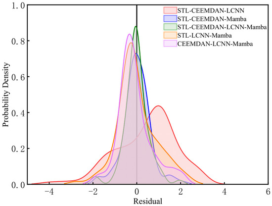
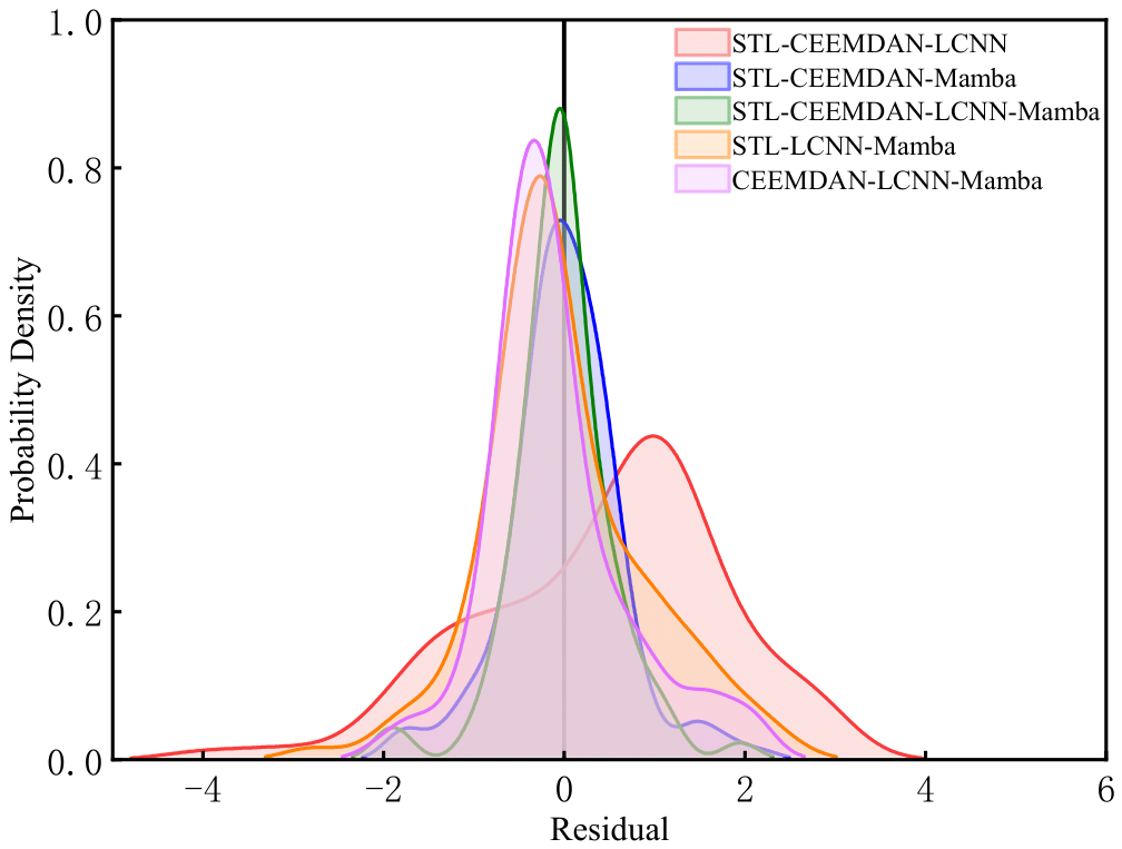
Table 5 lists the 90% confidence error interval and full-sample 100% residual range of all ablation models. The proposed STL-CEEMDAN-LCNN-Mamba obtains the narrowest residual bounds: its 90% error interval is [−0.8912, 0.8582], and the full residual range only spans [−2.2386, 2.2884]. By contrast, models missing any core module present drastically widened residual distribution ranges; the STL-CEEMDAN-LCNN baseline without Mamba owns the maximum residual span of [−4.8334, 3.9870], proving the Mamba unit greatly restricts extreme prediction bias. The residual probability density curve in Figure 12 further verifies the above conclusion. The green curve corresponding to our proposed model peaks closest to zero residual with the narrowest density envelope, meaning most prediction errors concentrate near 0. Other ablation models show wider, flatter density distributions, especially the red curve of STL-CEEMDAN-LCNN, whose residual density spreads far to both positive and negative directions, indicating frequent large deviation predictions.

Table 5. Residual distribution.

Predictive Model	90% Error Interval	100% Error Interval
STL-CEEMDAN-LCNN-Mamba	[−0.8912, 0.8582]	[−2.2386, 2.2884]
STL-CEEMDAN-Mamba	[−1.0304, 0.9136]	[−2.1799, 2.4071]
CEEMDAN-LCNN-Mamba	[−1.2784, 1.4795]	[−2.2883, 2.5173]
STL-LCNN-Mamba	[−1.3371, 1.4966]	[−3.3925, 2.9683]
STL-CEEMDAN-LCNN	[−1.8145, 2.5894]	[−4.8334, 3.9870]

Figure 12. Residual Probability Density Distribution.

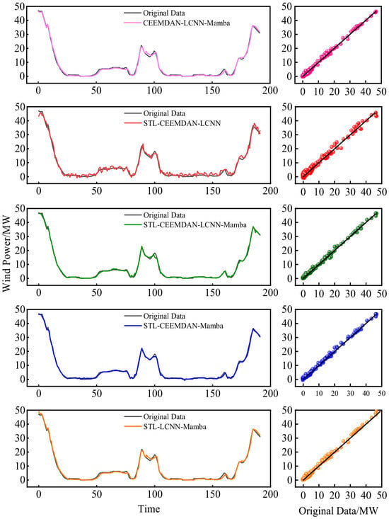
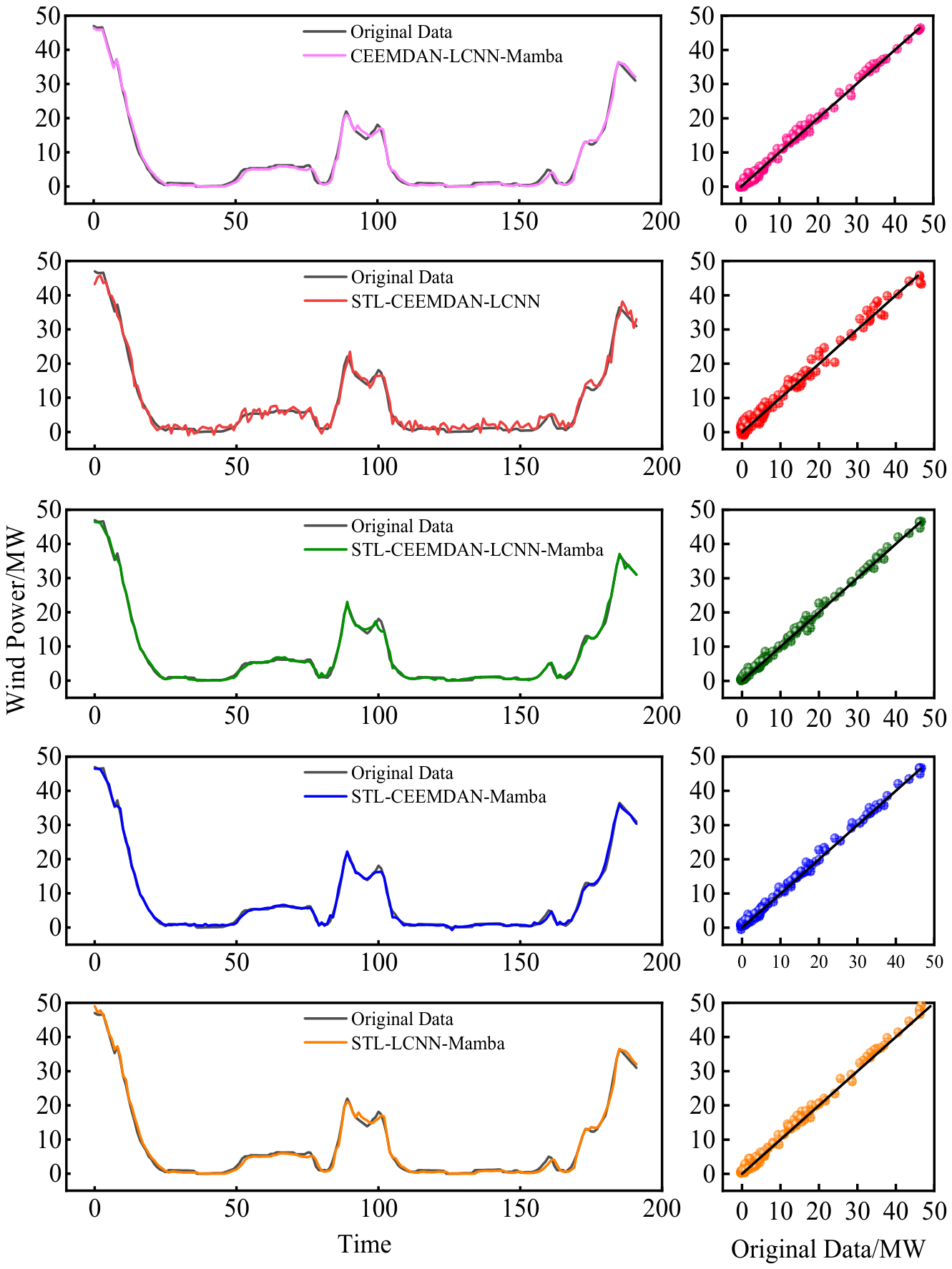
We plot the predicted wind power curves and corresponding correlation scatter plots of all ablation models in Figure 13 for intuitive visual comparison. where the colored scattered dots represent matching pairs of predicted and real wind power values, and the distance from each dot to the diagonal reference line reflects the prediction deviation degree of the model. Consistent with the quantitative metrics, the curve of STL-CEEMDAN-LCNN-Mamba nearly overlaps the original wind power series, and its scatter points tightly converge on the ideal diagonal reference line. By contrast, models missing STL, CEEMDAN, LCNN or Mamba modules show prominent deviations at power peaks and valleys, with scattered points far away from the diagonal, which indicates degraded fitting and generalization performance. Further comparison between CEEMDAN-LCNN-Mamba and the complete STL-CEEMDAN-LCNN-Mamba verifies the necessity of STL seasonal-trend decomposition: eliminating STL raises MAE from 0.418 to 0.580 and reduces R² to 0.957, because undecomposed raw wind power mixes intertwined trend, seasonal and noise components and increases prediction difficulty. Likewise, removing CEEMDAN (STL-LCNN-Mamba) expands residual ranges and enlarges prediction errors, proving that the two-stage STL-CEEMDAN decomposition can decouple mixed signals and lower forecasting complexity. The STL-CEEMDAN-LCNN baseline without Mamba achieves the worst overall performance, with MAE up to 0.933 and R² dropping to 0.979. Its prediction curve is plagued by violent oscillations, as standalone convolutional layers cannot efficiently capture long-range temporal dependencies and tend to introduce redundant noise, thereby impairing the model’s prediction stability and robustness.

Figure 13. Predicted Curves and Scatter Plots from Ablation Experiments.

Table 6 summarizes the averaged quantitative forecasting metrics (MAE, MSE, RMSE, R²) of five ablation models with five repeated random seed runs. Comparing STL-CEEMDAN-Mamba and the complete STL-CEEMDAN-LCNN-Mamba, we observe that embedding the LCNN convolution block delivers steady performance gains: MAE, MSE and RMSE drop by 7.1%, 3.7% and 2.3% separately, while R² rises from 0.989 to 0.996. Although the pure Mamba backbone already captures global long-term wind power trends well, it tends to over-smooth flat segments and fails to reconstruct tiny local fluctuations. The LCNN module compensates this defect by extracting fine-grained local sequence features, aligning predicted curves more closely with subtle power oscillations.

Table 6. Performance metrics for ablation experiments.

Predictive Model	MAE	MSE	RMSE	${\mathbf{R}}^2$
STL-CEEMDAN-LCNN-Mamba	0.418 ± 0.012	0.422 ± 0.015	0.647 ± 0.019	0.996 ± 0.002
STL-CEEMDAN-Mamba	0.450 ± 0.013	0.438 ± 0.013	0.662 ± 0.016	0.989 ± 0.004
CEEMDAN-LCNN-Mamba	0.580 ± 0.018	0.619 ± 0.019	0.786 ± 0.025	0.957 ± 0.007
STL-LCNN-Mamba	0.632 ± 0.023	0.701 ± 0.019	0.837 ± 0.030	0.942 ± 0.005
STL-CEEMDAN-LCNN	0.933 ± 0.019	1.984 ± 0.024	1.409 ± 0.032	0.979 ± 0.005

Overall, STL two-stage decomposition, CEEMDAN signal decomposition, LCNN local feature extraction and Mamba global temporal modeling each carry irreplaceable functions. Individual modules have obvious inherent drawbacks, while the assembled STL-CEEMDAN-LCNN-Mamba model realizes complementary strengths of all components, minimizes residual errors, tightens residual distribution near zero, and achieves optimal wind power forecasting accuracy and stability. The joint qualitative and quantitative results fully validate the rationality and effectiveness of our proposed multi-component hybrid prediction framework.

3.5. Generalization Experiments for the LCNN-Mamba Model

To further validate the generalization performance of the proposed model in complex environments, this paper utilizes historical operational data from 35,040 observation points at a wind farm in Ningxia as the training dataset, with a sampling interval of 15 min. This dataset shares five variables including wind speed, wind direction, temperature, atmospheric pressure and relative humidity with the main experimental dataset. Consistent with the experimental setup, we only take wind speed and wind direction as model input features. The two wind farms are separated by a straight-line distance of over 500 kilometres, with an altitude difference of around 400 m. The Ningxia wind farm sits on semi-desert land characterised by arid weather and sparse vegetation, which differs remarkably from the grassland terrain where the Inner Mongolia experimental wind farm is located. The wind power range of this dataset spans from 0 to 100 MW, exhibiting greater fluctuations and more drastic changes, which imposes higher requirements on the model’s generalization ability and stability.

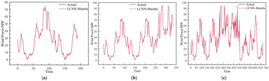
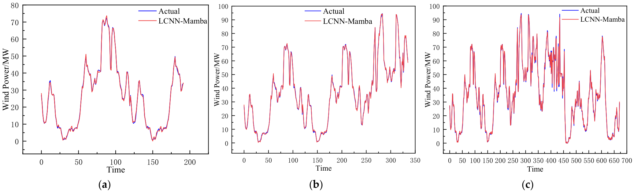
The prediction curves of the LCNN-Mamba model for different time steps are illustrated in Figure 14. Even when confronted with highly random and significantly fluctuating data, the model can still reasonably track the trends of the actual values. The 192-step and 336-step models perform better in regions with consecutive inflection points, closely matching the actual curve; the 672-step model shows slight lag at certain rapid change points. Although all three configurations exhibit a certain degree of error in regions with severe local fluctuations, the overall trend is accurately fitted without significant deviation or systematic distortion, indicating that the model possesses strong dynamic response capabilities under high-fluctuation scenarios.

Figure 14. Generalization results of the LCNN-Mamba model. (a) Prediction results for a 192-step time horizon; (b) Prediction results for a 336-step time horizon; (c) Prediction results for a 672-step time horizon.

As shown in Table 7, all three step-size models maintain high prediction accuracy. The short-step model achieves an RMSE of 0.63 and an R² of 0.996, yielding the smallest error and the best goodness-of-fit. The performance of the medium-step model takes second place with an R² of 0.957, while the long-step model obtains an R² of 0.908 and a relatively larger error. This indicates that under the current conditions of high fluctuation and strong uncertainty, a shorter time window is more conducive to capturing key variation characteristics. In summary, LCNN-Mamba, which relies on Mamba to capture global trends and LCNN to enhance local fitting, still demonstrates favorable generalization performance and stability in scenarios with expanded power ranges and intensified fluctuations.

Table 7. Generalization Performance of LCNN-Mamba Under Different Stride Lengths.

Prediction Step Size	MAE	MSE	RMSE	${\mathbf{R}}^2$
192	0.513 ± 0.018	0.402 ± 0.016	0.634 ± 0.025	0.996 ± 0.004
336	0.584 ± 0.015	0.558 ± 0.013	0.747 ± 0.016	0.957 ± 0.009
672	0.632 ± 0.020	0.670 ± 0.023	0.819 ± 0.029	0.908 ± 0.006

4. Conclusions

To advance sustainable wind energy exploitation and address the forecasting challenge of non-stationary wind power output time series, this paper combines the local feature extraction capability of LCNN with the long-sequence modeling capability of Mamba, proposing an LCNN-Mamba hybrid forecasting model based on STL-CEEMDAN secondary decomposition. Experimental validation leads to the following main conclusions:

(1)

Data processing stage: Applying the STL-CEEMDAN two-stage decomposition to the raw wind power time series—first separating the trend and seasonal components via STL, followed by CEEMDAN-based multiscale decomposition of the residual component—effectively reduces the non-stationarity and complexity of the series. Combined with a dominant frequency ordering and reconstruction strategy, this approach effectively organizes high- and low-frequency information, providing a clear and stable input representation for subsequent modeling. Comparative analysis reveals that this dual decomposition strategy has significant advantages in feature separation and information preservation.

(2)

Forecasting modeling stage: A hybrid LCNN-Mamba architecture is constructed to collaboratively learn multiscale features, where LCNN extracts local temporal patterns and short-term dynamic changes, while Mamba captures the long-term dependencies and global evolutionary characteristics of the series. Through feature mapping and residual mechanisms, information transmission losses are alleviated, which enhances the model’s training stability and convergence efficiency. Experimental results demonstrate that this method maintains excellent prediction accuracy and stability across various data scenarios, exhibiting stronger overall performance and adaptability compared to baseline models.

Although the proposed STL-CEEMDAN-LCNN-Mamba hybrid model achieves favorable prediction performance for multi-step wind power forecasting, the construction of its input feature system still has room for further optimization. Future work will introduce dedicated neural network modules to refine feature engineering processing, so as to fully mine the interactive coupling relationships between multi-meteorological variables and wind power output. From the perspective of practical power system engineering, this model can provide reliable power data support for wind farm dispatching, power grid operation and HVDC system regulation, showing important practical application value. In follow-up research, we will promote the model towards lightweight deployment and on-site application, and further validate its generalization performance on wind power datasets from southern China and other time-series forecasting fields.

References

- Zhu, P.; Ma, Y.; Chen, X.; Li, H. Explore Green Land Use Against the Background of Carbon Peaking and Carbon Neutrality: Take Wind and Solar Power Generation as Examples. Macroecon. Manag. 2024, 11, 45–51. [Google Scholar] [CrossRef]
- Zha, W.T.; Liu, J.; Li, Y.L.; Liang, Y.Y. Ultra-short-term power forecast method for the wind farm based on feature selection and temporal convolution network. ISA Trans. 2022, 129, 405–414. [Google Scholar] [CrossRef] [Scilit] [PubMed]
- Wang, J.J.; Shu, S.Q.; Xu, S.L. A point-interval wind speed prediction model based on entropy clustering and hybrid optimization weighted strategy. Renew. Energy 2025, 244, 122653. [Google Scholar] [CrossRef] [Scilit]
- Liu, K.; Li, B.; Jiang, Q.; Zhang, Y.; Liu, T. Fault ride-through strategy for hybrid cascaded HVDC systems based on controllable LCC. IEEE Trans. Circuits Syst. II Express Briefs 2025, 73, 88–92. [Google Scholar] [CrossRef] [Scilit]
- Li, T.; Ai, L.J.; Yang, Q.S.; Zhang, X.X.; Li, H.; Lu, D.W.; Shen, H.T. Short-term wind power prediction based on multiscale numerical simulation coupled with deep learning. Renew. Energy 2025, 246, 122951. [Google Scholar] [CrossRef] [Scilit]
- He, Y.; Wang, W.; Li, M.; Wang, Q.H. A short-term wind power prediction approach based on an improved dung beetle optimizer algorithm, variational modal decomposition, and deep learning. Comput. Electr. Eng. 2024, 116, 109182. [Google Scholar] [CrossRef] [Scilit]
- Huang, M. Analysis of Wind Power Technology and Photovoltaic Power Generation Technology. Instrum. Technol. Users 2025, 32, 138–140. [Google Scholar]
- Sun, R.; Zhang, T.; He, Q.; Xu, H. Review on Key Technologies and Applications in Wind Power Forecasting. High Volt. Eng. 2021, 47, 1129–1143. [Google Scholar] [CrossRef]
- Medsker, L.R.; Jain, L. Recurrent neural networks. Des. Appl. 2001, 5, 64–67. [Google Scholar]
- Graves, A. Long short-term memory. In Supervised Sequence Labelling with Recurrent Neural Networks; Springer: Berlin/Heidelberg, Germany, 2012; pp. 37–45. [Google Scholar]
- Cheng, M.; Qian, W.; He, X. The Research on Wind Power Prediction Based on Wind Speed Correction. In Proceedings of the 2023 42nd Chinese Control Conference (CCC); IEEE: Piscataway, NJ, USA, 2023; pp. 6309–6314. [Google Scholar] [CrossRef] [Scilit]
- Zhang, Y.M.; Wang, H. Multi-Head Attention-Based Probabilistic CNN-BiLSTM for Day-Ahead Wind Speed Forecasting. Energy 2023, 278, 127865. [Google Scholar] [CrossRef] [Scilit]
- Zhao, Z.; Yun, S.; Jia, L.; Guo, J.; Meng, Y.; He, N.; Li, X.; Shi, J.; Yang, L. Hybrid VMD-CNN-GRU-Based Model for Short-Term Forecasting of Wind Power Considering Spatio-Temporal Features. Eng. Appl. Artif. Intell. 2023, 121, 105982. [Google Scholar] [CrossRef] [Scilit]
- Jiang, B.; Yang, H.; Wang, Y.; Wang, Q.; Geng, H. Transfer Learning-Based Model Training for Short-Term Load Forecasting. J. Mod. Power Syst. Clean Energy 2025, 14, 590–601. [Google Scholar] [CrossRef] [Scilit]
- Jiang, B.; Yang, H.; Wang, Q.; Wang, Y.; Geng, H. Multitask learning for enhanced short-term load forecasting in distribution networks under small sample conditions. CSEE J. Power Energy Syst. 2025, 1–10. [Google Scholar]
- Chen, H.; Wang, Y.; Guo, T.; Xu, C.; Deng, Y.; Liu, Z.; Ma, S.; Xu, C.; Xu, C.; Gao, W. Pre-trained image processing transformer. In Proceedings of the IEEE/CVF Conference on Computer Vision and Pattern Recognition, Nashville, TN, USA, 20–25 June 2021; pp. 12299–12310. [Google Scholar]
- Hofstätter, S.; Zamani, H.; Mitra, B.; Craswell, N.; Hanbury, A. Local self-attention over long text for efficient document retrieval. In Proceedings of the 43rd International ACM SIGIR Conference on Research and Development in Information Retrieval, Virtual Event, 25–30 July 2020; p. 2021. [Google Scholar]
- Wu, N.; Green, B.; Ben, X.; O’Banion, S. Deep transformer models for time series forecasting: The influenza prevalence case. arXiv 2020, arXiv:2001.08317. [Google Scholar]
- Huang, S.; Yan, C.; Qu, Y. Deep Learning Model-Transformer Based Wind Power Forecasting Approach. Front. Energy Res. 2023, 10, 1055683. [Google Scholar] [CrossRef] [Scilit]
- Zhou, H.; Zhang, S.; Peng, J.; Zhang, S.; Li, J.; Xiong, H.; Zhang, W. Informer: Beyond Efficient Transformer for Long Sequence Time-Series Forecasting. Proc. AAAI Conf. Artif. Intell. 2021, 35, 11106–11115. [Google Scholar] [CrossRef] [Scilit]
- Rangapuram, S.S.; Seeger, M.W.; Gasthaus, J.; Stella, L.; Wang, Y.; Januschowski, T. Deep State Space Models for Time Series Forecasting. Adv. Neural Inf. Process. Syst. 31 (NeurIPS 2018) 2018, 31, 7785–7794. [Google Scholar]
- Gu, A.; Dao, T. Mamba: Linear-time sequence modeling with selective state spaces. arXiv 2023, arXiv:2312.00752. [Google Scholar]
- Wang, Y.S.; Pei, L.L.; Li, W.; Zhao, Y.L.; Shan, Y.H. Short-Term Wind Power Prediction Method Based on Multivariate Signal Decomposition and RIME Optimization Algorithm. Expert Syst. Appl. 2025, 259, 125376. [Google Scholar] [CrossRef] [Scilit]
- Liu, Y. A Wind Speed Prediction Method Based on Signal Decomposition Technology Deep Learning Model. Energies 2025, 18, 1136. [Google Scholar] [CrossRef] [Scilit]
- Peng, T.; Jin, J.; Wang, D. Enhanced Wind Speed Forecasting Using Fractal-Guided Signal Decomposition and Optimized Gated Recurrent Unit for Wind Energy Integration. Sustain. Energy Technol. Assess. 2025, 84, 104754. [Google Scholar] [CrossRef] [Scilit]
- Wu, Z.; Huang, N.E. Ensemble Empirical Mode Decomposition: A Noise-Assisted Data Analysis Method. Adv. Adapt. Data Anal. 2009, 1, 1–41. [Google Scholar] [CrossRef] [Scilit]
- Li, H.; Ye, X.; Fu, G. Review on the Application of Signal Decomposition Technology in Power Prediction of New Energy Power Generation. South. Power Syst. Technol. 2023, 17, 3–15. [Google Scholar] [CrossRef]
- Dragomiretskiy, K.; Zosso, D. Variational Mode Decomposition. IEEE Trans. Signal Process. 2014, 62, 531–544. [Google Scholar] [CrossRef] [Scilit]
- Xiang, L.; Liu, J.; Su, H.; Hu, A.; Zhu, Z. Research on Multi-Step Wind Speed Forecast Based on CEEMDAN Secondary Decomposition and LSTM. Acta Energiae Solaris Sin. 2022, 43, 334–339. [Google Scholar] [CrossRef]
- Wang, B.W.; Huang, Y.; Meng, Z.B.; Cao, S.T. Research on Port Container Throughput Forecasting Based on Secondary Decomposition and LSTM Optimized by Algorithm. Navig. China 2025, 48, 121–131. [Google Scholar]
- Sun, Z.; Zhao, M.; Dong, Y.; Cao, X.; Sun, H. Hybrid Model with Secondary Decomposition, Random Forest Algorithm, Clustering Analysis and Long Short Memory Network Principal Computing for Short-Term Wind Power Forecasting on Multiple Scales. Energy 2021, 221, 119848. [Google Scholar] [CrossRef] [Scilit]
- Jin, Z.; Fu, X.; Xiang, L.; Zhu, G.; Hu, A. Informer Learning Framework Based on Secondary Decomposition for Multi-Step Forecast of Ultra-Short Term Wind Speed. Eng. Appl. Artif. Intell. 2025, 139, 109702. [Google Scholar] [CrossRef] [Scilit]
- Lei, P.; Ma, F.; Zhu, C.; Li, T. LSTM Short-Term Wind Power Prediction Method Based on Data Preprocessing and Variational Modal Decomposition for Soft Sensors. Sensors 2024, 24, 2521. [Google Scholar] [CrossRef] [Scilit] [PubMed]
- Ding, J.W.; Chuang, M.J.; Tseng, J.S.; Hsieh, I.Y.L. Reanalysis and Ground Station Data: Advanced Data Preprocessing in Deep Learning for Wind Power Prediction. Appl. Energy 2024, 375, 124129. [Google Scholar] [CrossRef] [Scilit]
- Li, D.; Tang, J.; Liao, S.W.; Huang, F.Y.; Luo, J.J. Ultra-Short-Term Wind Power Prediction Considering Dynamic Interpolation of Missing Values of Time Series Features. Proc. CSEE 2025, 45, 6790–6804. [Google Scholar] [CrossRef]
- Zang, X.; Wang, Z.; Zhang, S.; Bai, M. Short-Term Wind Power Prediction Based on MVMD-AVOA-CNN-LSTM-AM. Int. Trans. Electr. Energy Syst. 2025, 2025, 3570731. [Google Scholar] [CrossRef] [Scilit]
- Li, D.A.; Bai, X.D.; Xia, H.W.; Feng, D. Short-and Medium-Term Photovoltaic Power Prediction Based on STL-Former. J. Eng. Therm. Energy Power 2024, 39, 140–146+153. [Google Scholar] [CrossRef]
- Li, Z.; Ye, Y.; Liu, W.; Lu, A. Short-Term Wind Power Prediction Based on STL-AOA-Transformer Algorithm. In Proceedings of the 2024 9th International Conference on Power and Renewable Energy (ICPRE), Guangzhou, China, 20–23 September 2024; pp. 1390–1395. [Google Scholar]
- Han, B.; Li, C.Q.; Liu, W.L.; Liu, S.; Liu, C.L.; Xu, J.H.; Wang, X. Ultra-Short-Term Photovoltaic Power Forecasting Based on Secondary Decomposition and BiGRU. J. Chin. Soc. Power Eng. 2025, 45, 62–69+79. [Google Scholar] [CrossRef]
- Karijadi, I.; Chou, S.Y.; Dewabharata, A. Wind Power Forecasting Based on Hybrid CEEMDAN-EWT Deep Learning Method. Renew. Energy 2023, 218, 119357. [Google Scholar] [CrossRef] [Scilit]
- Wang, Z.; Wang, Y.; Wang, H.; Tang, N.; Wang, S. Integrating Fast Iterative Filtering and Ensemble Neural Network Structure with Attention Mechanism for Carbon Price Forecasting. Complex Intell. Syst. 2025, 11, 1609. [Google Scholar]
- Li, J.; Liu, M.; Wen, L.; Tian, Z.; Ramirez, C.A.P. Forecasting Model for Short-Term Wind Speed Using Robust Local Mean Decomposition, Deep Neural Networks, Intelligent Algorithm, and Error Correction. Front. Energy Res. 2024, 11, 1336675. [Google Scholar] [CrossRef] [Scilit]
- Wang, Z.; Kong, F.; Feng, S.; Wang, M.; Yang, X.; Zhao, H.; Wang, D.; Zhang, Y. Is Mamba Effective for Time Series Forecasting? Neurocomputing 2025, 619, 129178. [Google Scholar] [CrossRef] [Scilit]
Disclaimer/Publisher’s Note: The statements, opinions and data contained in all publications are solely those of the individual author(s) and contributor(s) and not of MDPI and/or the editor(s). MDPI and/or the editor(s) disclaim responsibility for any injury to people or property resulting from any ideas, methods, instructions or products referred to in the content. |
© 2026 by the authors. Licensee MDPI, Basel, Switzerland. This article is an open access article distributed under the terms and conditions of the Creative Commons Attribution (CC BY) license.