


Abstract
Energy poverty poses a critical threat to global sustainable development by undermining household well-being and deepening social inequality. This study draws on data from 17,778 households across six waves of the China Family Panel Studies (CFPS) from 2012 to 2022 to examine the dynamics, determinants, and predictive patterns of household energy poverty in China. Our study also enhances and optimises the four-quadrant classification framework within the Low-Income, High-Cost (LIHC) framework, which jointly evaluates income and energy expenditure using dynamic thresholds. This approach enables us to identify not only households experiencing energy poverty but also those facing heightened vulnerability. In the sample, 7.96% were classified as energy-poor, 29.10% as at risk of energy poverty, 24.14% as at risk of income poverty, and 38.81% as not at risk, indicating that the number of households facing hidden risks far exceeds that of households identified as poor using traditional binary diagnostic methods. Next, we implement a Bayesian-optimised Extreme Gradient Boosting (XGBoost) model to improve predictive accuracy. Thus, the trained model achieved a prediction accuracy of 78%. We employ Shapley Additive exPlanations (SHAP) analysis to interpret the relative importance and interaction of explanatory variables. Our findings reveal three key patterns. First, households at risk of energy insecurity substantially outnumber those already in energy poverty, indicating a large latent vulnerable population that conventional measures often overlook. Second, housing conditions and energy expenditures remain the dominant structural drivers of energy poverty; however, financial pressures related to healthcare, education, and other non-energy expenditures increasingly intensify vulnerability. Third, Bayesian optimisation significantly enhances the model’s capacity to capture nonlinear relationships and complex household heterogeneity. By integrating dynamic measurement with interpretable machine learning, this study advances methodological approaches to energy poverty assessment and provides robust empirical evidence for early-warning systems, differentiated governance strategies, and targeted policy design in the context of China’s energy transition.
1. Introduction
Energy poverty poses a serious barrier to sustainable development because it undermines human well-being and exacerbates social inequality. The United Nations incorporated access to affordable and clean energy into the 2030 Agenda for Sustainable Development as a core development objective, underscoring its central role in poverty reduction and low-carbon transition strategies [1]. Governments cannot achieve inclusive growth or climate goals without addressing persistent disparities in household energy access and affordability. Household energy poverty manifests differently across development contexts. In many parts of sub-Saharan Africa and South Asia, limited physical access to electricity and clean cooking fuels remains the primary challenge [2]. In contrast, developed economies largely achieve universal access but struggle with affordability. Low-income households often face high energy costs due to inefficient housing, stagnant wages, and volatile energy prices, which push them into energy poverty despite formal access [3]. Even within developing countries, energy poverty is not uniformly distributed since it displays significant multidimensional variation. It varies sharply across urban–rural divides, social groups, regions, and demographic groups, reflecting multidimensional structural inequalities [4].
Several scholars have consistently measured energy poverty using the 10% expenditure rule or the Low-Income–High-Cost (LIHC) indicator proposed by Hills [5]. The LIHC framework conceptualises a four-quadrant space defined by income and energy expenditure thresholds and provides a structured approach to identifying energy-poor households. However, most empirical applications reduce this framework to a static binary classification, labelling households as either “energy-poor” or “non-energy-poor.” This binary approach underutilises the conceptual richness of the four-quadrant design and obscures households that face only one dimension of risk—low income or high energy burden. As a result, many vulnerable households remain analytically invisible, and policy responses overlook emerging risks [6]. At the same time, most studies rely on traditional econometric models to explain energy poverty ex post. While these approaches identify correlates, they rarely provide forward-looking risk prediction or uncover nonlinear interactions among determinants [7,8]. Consequently, policymakers often respond to energy poverty after it materialises rather than preventing it through early warning systems. Bridging this gap requires integrating refined measurement frameworks with predictive and interpretable analytical tools.
China offers a particularly important case for such analysis. As the world’s largest developing country, China simultaneously confronts massive energy demand and pronounced regional disparities. Its household energy poverty reflects both access-related challenges typical of developing economies and efficiency and affordability pressures associated with low-carbon transition pathways. Although the urban–rural energy access gap has narrowed significantly, rural households continue to bear disproportionate transition costs [2]. Social capital mitigates vulnerability unevenly across groups, and the poverty-reduction effects of energy efficiency improvements differ by region [9]. Moreover, a substantial share of households still rely on traditional biomass fuels, exposing them to health risks and limiting clean energy adoption [10]. This layered heterogeneity makes China an ideal context for examining the dynamic evolution and risk stratification of household energy poverty. Against this background, we analyse six waves (2012–2022) of panel data from the China Family Panel Studies (CFPS). The CFPS dataset provides nationally representative, longitudinal, and multidimensional information on household income, energy expenditure, housing conditions, and demographic characteristics. Its panel structure enables us to track vulnerability trajectories and capture dynamic risk transitions over time.
We structure our research around three methodological innovations. First, we refine the LIHC analytical framework by constructing a dynamic four-quadrant classification system with dual thresholds for income and expenditure. Instead of collapsing the framework into a binary outcome, we categorise households into four distinct risk statuses: risk-free, income-at-risk, energy-at-risk, and energy-poor. This design enables granular and dynamic identification of both realised and latent vulnerability conditions. Second, we apply a Bayesian-optimised XGBoost machine learning model to predict household energy poverty. By systematically tuning hyperparameters, we improve classification performance and strengthen early-warning capacity. Third, we employ SHAP analysis to interpret the model’s predictions. This approach quantifies each feature’s marginal contribution and reveals nonlinear interactions among determinants, thereby transforming predictive modelling from a “black box” exercise into an interpretable governance tool. This study contributes to the literature in two principal ways.
Firstly, drawing on the theoretical framework of the Low-Income–High-Cost (LIHC) model, this paper integrates income risk with energy affordability risk and, by setting dynamic thresholds, constructs a comprehensive risk map of energy vulnerability among Chinese households. Compared to the traditional binary (energy-poor/non-energy-poor) classification, this approach identifies ‘potentially vulnerable’ households (such as those with high incomes but high energy costs), thereby expanding the empirical application of the LIHC framework in the context of developing countries, offering a practical improvement for measuring multidimensional energy poverty.
Secondly, this study combines a Bayesian-optimised XGBoost model with the SHAP interpretation tool for the prediction and mechanism analysis of household energy poverty. This marks a fundamental shift from ‘post-event explanation’ to ‘pre-event prediction and mechanism analysis’. Compared to traditional econometric models, such as logistic regression, this method can reveal non-linear interaction effects between variables. This combined approach strikes a good balance between predictive accuracy and model interpretability, providing an analytical tool for dynamic screening and targeted intervention in energy poverty.
2. Literature Review
2.1. From Fuel Poverty to Multidimensional Energy Poverty
Several scholars have widely recognised energy poverty as a global household challenge, yet they have not reached a universally accepted definition [11]. Boardman first introduced the concept of “fuel poverty,” defining households that spend more than 10% of their income on fuel as fuel-poor and identifying low income, rising energy prices, and poor housing efficiency as primary drivers [12]. This definition linked energy deprivation directly to affordability constraints in heating and basic domestic energy services. As energy systems diversified and electricity and clean fuels became central to development, researchers expanded the framework from “fuel poverty” to “energy poverty.” This broader concept captures both accessibility and affordability across multiple energy services [13]. From a sociological perspective, some notable scholars further argue that energy poverty reflects a household’s inability to secure the material and social energy services necessary for dignified living and long-term development [14]. This shift repositioned energy poverty as a multidimensional deprivation rather than a narrow expenditure ratio.
Measurement approaches evolved in parallel. Early single-dimensional indicators—particularly the 10% rule—offered operational simplicity but often misclassified high-income households with high consumption as energy-poor. The LIHC indicator improved precision by jointly comparing income to poverty thresholds and energy expenditure to median needs [5]. Additional refinements, such as minimum energy requirement thresholds, further strengthened identification logic. More recently, some scholars have developed multidimensional indices, including the Energy Development Index (EDI), the Multidimensional Energy Poverty Index (MEPI), and the Energy Poverty Index (EPI) [15,16]. These approaches integrate multiple deprivation dimensions, such as access, affordability, and service quality. However, both fixed-threshold single indicators and composite indices struggle to account for contextual heterogeneity across regions with varying income levels, energy prices, and development stages [17]. Consequently, measurement frameworks often fail to capture dynamic vulnerability and transitional risk.
2.2. A Multidimensional Macro Research Framework on Energy Poverty
With the advancement of the Sustainable Development Goals (SDGs), researchers have increasingly embedded energy poverty within a broader macro-level framework that integrates economic development, governance, regional inequality, and energy transition. From an economic perspective, studies consistently show that energy poverty undermines sustainable growth and reduces subjective well-being. This relationship varies across income groups and time horizons, requiring dimension-specific policy responses [18,19]. Energy poverty not only constrains productivity but also reinforces social inequality.
In the policy domain, scholars demonstrate that renewable energy promotion, efficiency upgrades, and targeted subsidies can alleviate energy poverty. However, governance effectiveness depends on institutional coordination, regional alignment, and precise targeting [20]. Without adaptive governance systems, policy interventions often generate uneven outcomes.
Spatial analyses further reveal significant regional heterogeneity and spillover effects. Some researchers have emphasised the need for differentiated infrastructure investment and coordinated regional strategies to reduce persistent disparities [9]. Comparative studies also identify interconnections between energy poverty and transportation poverty, suggesting that policy priorities must align with national development stages [21].
Notably, some scholars have examined the interaction between energy transition and poverty alleviation. More importantly, they find that low-carbon transitions can either alleviate or exacerbate energy poverty, depending on energy structure, development stage, and complementary policies. Achieving a dual objective of decarbonization and poverty reduction requires targeted subsidies and efficiency improvements tailored to regional needs [22]. Nevertheless, although macro-level research provides valuable insights into structural drivers and policy pathways, it rarely investigates how household-level heterogeneity shapes vulnerability trajectories.
2.3. Micro-Level Household Energy Poverty Gaps and Constraints
As the core micro-unit in energy poverty governance, several studies on household energy poverty have recognised households as the fundamental governance unit of energy poverty. However, a systematic framework for analysing underlying mechanisms has not yet been established. This entails that both the depth and specificity of such research require further enhancement. Expectedly, micro-level studies consistently identify income level and energy expenditure share as core determinants [23]. In addition, housing quality and infrastructure inefficiency further intensify vulnerability by creating a reinforcing cycle of poor conditions, high consumption, and financial strain [24].
From a global research perspective, existing studies on energy poverty predominantly adopt macro perspectives, focusing primarily on macro-level economic linkages and energy transition effects [19,22], as well as regional-scale variations in energy poverty and spatial spillover characteristics [9]. Comparatively, most studies stop at establishing statistical associations. They rarely construct systematic frameworks to analyse transmission pathways, interaction mechanisms, or dynamic transitions. Also, several macro-oriented studies treat household energy poverty as an aggregated component of regional poverty, overlooking how micro-level heterogeneity—such as income structure, housing conditions, and consumption trade-offs—shapes risk formation [25]. As a result, existing research fails to explain how multiple pressures jointly push households from vulnerability into persistent energy poverty [26]. These limitations become more pronounced in developing countries since households often rely on traditional biomass fuels, face unstable electricity infrastructure, and experience volatile income streams [27].
Without micro-level mechanism analysis, policymakers struggle to design effective interventions. Subsidies and retrofit programmes may miss genuinely vulnerable households because researchers have not clarified the causal and interactive pathways underlying risk [28]. Furthermore, weak predictive capacity limits early warning systems, making it difficult to identify households at transitional stages before poverty materialises [26]. To improve governance precision, researchers need to systematically analyse how diverse household characteristics interact dynamically and generate differentiated vulnerability pathways.
2.4. Machine Learning Methods in Energy Poverty Research
Recent advances in big data and artificial intelligence have expanded methodological tools in energy poverty research. For instance, numerous studies increasingly apply machine learning prediction models such as random forests, support vector machines, gradient boosting trees, and ensemble methods to improve prediction and targeting accuracy [29]. Using random forests (as opposed to logistic regression) to analyse complex multidimensional household determinants in the Netherlands [30] and applying decision tree models to evaluate energy efficiency drivers in institutional settings [31] was found to be a more effective method. Likewise, energy poverty prediction models were constructed using ensemble learning methods such as random forest and gradient boosting, combined with socioeconomic impact factor datasets [32].
These models offer flexibility and relatively low development costs, making them suitable for preliminary analysis and moderate-sized datasets. However, they present limitations. Random forests may overfit without regularisation and struggle with high-dimensional sparse data. Logistic regression cannot capture complex nonlinear interactions. Intriguingly, support vector machines often perform poorly in large-scale or highly heterogeneous datasets. Among these approaches, XGBoost offers notable advantages. It efficiently processes large datasets, performs automatic feature selection, incorporates regularisation, and captures nonlinear relationships with high predictive performance [29]. Several studies have combined XGBoost with spatial autocorrelation analysis—using the Global Moran’s I index—to map and forecast regional energy poverty risks [33]. Others have used it to analyse electricity consumption patterns among vulnerable groups [34].
While existing literature on the use of machine learning to study household energy poverty has made some significant inroads into mainstream literature, there is still room for further development. Firstly, in the field of predictive modelling, most research focuses on improving predictive accuracy, treating machine learning models as ‘black boxes’, with relatively less attention paid to model interpretability. Secondly, the scarcity of research integrating system parameter optimisation (such as Bayesian optimisation) with interpretability tools (such as SHAP), particularly in the context of developing countries, informs studies in this focal area. Based on the abovementioned observations, we observe that there is still a wide scope for further exploration in existing research areas across the following three dimensions: (1) The empirical application of multi-dimensional classification frameworks in identifying household energy vulnerability in developing countries can be further explored; (2) Micro-level mechanism analyses tailored towards the context of developing countries (particularly regarding the relationship that exists between housing conditions, expenditure patterns, and non-linear pathways to energy poverty) require more detailed empirical testing; (3) The integration of predictive accuracy with interpretability in machine learning methods applied to research on energy poverty is still in its infancy.
3. Materials and Methods
3.1. Data Sources
We draw on data from the CFPS, a nationally representative longitudinal survey covering 25 provinces, autonomous regions, and municipalities across China. The CFPS provides rich household-level information on income, consumption, housing conditions, demographic characteristics, and social factors, making it particularly suitable for energy poverty analysis. Given that certain key variables were unavailable before 2012 and the latest publicly available released wave is 2022, we construct a balanced six-wave panel dataset covering the period 2012–2022. The biennial survey structure allows us to observe medium-term transitions in household economic and energy conditions. Notably, the dataset includes household income, disaggregated energy expenditures, population size, health status, medical insurance coverage, housing characteristics, and geographical location. All data were processed and analyzed using Stata version 18. We clean the dataset by removing extreme outliers and imputing missing values using consistent panel procedures. After data processing, we retain 17,778 valid household observations. This sample provides a robust empirical foundation for dynamic identification and predictive modelling of household energy poverty.
3.2. Classification Framework
Based on the LIHC metric, we have extended a dynamic four-quadrant classification framework. The framework hinges on two carefully calibrated thresholds: a household income threshold and an energy expenditure threshold.
(1) Income Threshold
Previous international research on energy poverty, including those involving case studies from the Netherlands and the United Kingdom have consistently identified household disposable income as the core determinant of energy affordability. In this study, we define household net income as the horizontal (x-axis) dimension of the framework. Concurrently, relative poverty measurement commonly sets the threshold at 40%, 50%, or 60% of median income, depending on the economic context [35].
For instance, developed economies, such as the European Union (EU) member states, frequently adopt a 60% threshold to define relative poverty. However, applying such a high benchmark in developing nations with pronounced income inequality risks overextending the poverty classification and weakening policy targeting [36,37]. OECD countries often use 50% as a transitional benchmark in relatively balanced income systems [38], yet empirical evidence from middle-income economies shows that this threshold substantially enlarges the poverty population and increases fiscal pressure. Conversely, lower thresholds (e.g., 35%) identify households close to absolute poverty but fail to capture vulnerable groups living just above the poverty line [39]. In China, a large share of households occupy this “near-poor” category: their incomes exceed the absolute poverty line but remain highly sensitive to shocks. To reflect China’s developmental stage and vulnerability structure, we set the income threshold at 40% of the median income plus necessary energy expenditure. This threshold balances precision targeting with recognition of transitional vulnerability [18].
(2) Energy Expenditure Threshold
We define the vertical (y-axis) dimension as the ratio of household energy expenditure to income. The energy expenditure share remains the most widely used operational indicator of energy burden [40,41]. Boardman’s “10% rule” historically defined households spending more than 10% of income on energy as energy-poor [12], and EU research continues to rely on expenditure ratios as a core affordability measure [42]. To refine this threshold in a dynamic and context-sensitive manner, we draw on the classical Environmental Kuznets Curve (EKC) logic, which posits an inverted U-shaped relationship between per capita income and environmental resource consumption [43]. Applied to household energy use, this framework suggests that energy expenditure shares initially rise during income growth as households improve their living standards. After reaching a certain income level, households invest in efficiency improvements, causing the energy expenditure share to decline.
Furthermore, the group within society exhibiting the most rational energy consumption and bearing the most reasonable burden should theoretically be situated near the inflexion point of this inverted U-shaped curve. For instance, households that have satisfied their basic energy needs but have not yet entered the stage of luxury energy consumption should be included in this category. Empirical studies in China confirm this pattern: as income rises, households initially increase energy consumption to enhance living standards before subsequently prioritising energy efficiency improvements [44]. Middle-income households often occupy the “expansion stage,” during which energy expenditure constitutes a relatively high budget share. This group plays a critical role in energy transition dynamics and warrants special policy attention. Based on this logic, we set the energy expenditure threshold at the median proportion of income allocated to energy among households with incomes hovering between 40% and 60% of the overall median income. This benchmark reflects the expenditure level associated with structurally typical, non-luxury energy consumption in transitional income groups.
Although the threshold settings for the classification framework are supported by the aforementioned literature, we have also conducted additional robustness tests for the alternative thresholds mentioned above and compared the classification results with the absolute poverty line to confirm that the threshold-based classification framework used in this study is robust. The specific details are presented in the Appendix A (Table A1, Table A2 and Table A3, and Figure A1).
As illustrated in Figure 1, based on the aforementioned income and expenditure thresholds, we construct a four-quadrant classification system that captures both realised and latent vulnerability. We, therefore, categorise households energy poverty into four risk levels: no risk, income risk, energy risk, and dual risk. Households experiencing dual risk are classified as energy-poor households. Specifically, households with income at or above the income threshold and energy expenditure below the expenditure threshold are classified as the non-risk category. While those with income below the income threshold but energy expenditure below the expenditure threshold are classified as the income-risk category. Whereas those with income at or above the income threshold but energy expenditure above the expenditure threshold are classified as the energy-risk category. Likewise, those with both income below the income threshold and energy expenditure above the expenditure threshold are classified as the energy poverty (dual-risk) category [30].
Figure 1.
Dual-Threshold Classification Framework for Income and Energy Expenditure.
Furthermore, households in the dual-risk quadrant experience simultaneous income insufficiency and excessive energy burden; we classify them as energy-poor. Unlike binary identification approaches, this framework explicitly distinguishes between structural income vulnerability and excessive energy burden, enabling granular risk mapping and early-warning identification. By applying the full conceptual scope of the LIHC framework, we avoided static diagnostics to extend a dynamic, policy-relevant hierarchical system designed to support targeted governance and predictive modelling.
3.3. Variable Selection
We organise the variables into two principal categories. First, we select categorical framework variables that determine a household’s position within the four-quadrant risk framework. Second, we include multidimensional household-level variables for characteristic analysis, model training, and interpretation of predictive mechanisms. Together, these variables form a comprehensive identification system that supports precise measurement and prediction of household energy poverty.
To enhance methodological transparency, the study explicitly defines the computation of dynamic income and energy expenditure thresholds, including whether thresholds are determined annually using sample percentiles or anchored to inflation-adjusted national medians. This clarification ensures replicability and facilitates cross-study comparability.
(1) Classification Variables
We ground the classification variables in the LIHC framework, which defines energy poverty through the dual characteristics of low income and high energy expenditure. Consistent with this theoretical structure, we select household net income and energy expenditure as the core identification variables. This choice aligns international energy poverty theory with China’s specific income distribution patterns and household energy expenditure structure.
(2) Multidimensional Household Characteristics
To capture the complexity of energy vulnerability, we incorporate variables across multiple dimensions. Demographic characteristics (e.g., household size, age structure, gender composition) reflect household energy consumption needs and resilience capacity. For instance, larger households typically exhibit higher energy demand [45]. Geographical and regional variables (urban/rural status, province, region) capture structural disparities in infrastructure and energy access. Differences in supply modes, climate conditions, and development levels can significantly affect household energy burdens [46]. Economic and expenditure structure variables (total income, total expenditure, disaggregated energy and non-energy spending) reveal the trade-offs households make between energy and other essential goods. Energy access and consumption variables (fuel type, cooking energy source, electrification status) directly represent household energy usage patterns and service quality [47]. By integrating these dimensions, we move beyond single-factor analysis and construct a multidimensional explanatory framework capable of identifying both structural drivers and interaction effects. The complete list of variables appears in Table 1.
Table 1.
Variable System Influencing Energy Poverty.
3.4. Model Configuration
We employ the XGBoost algorithm as our primary predictive model. XGBoost improves upon traditional gradient boosting by incorporating regularisation, second-order optimisation, and efficient parallel computation. These enhancements enable the model to process high-dimensional data and capture complex nonlinear relationships—features that are essential for identifying heterogeneous energy poverty risks [32]. We also used the Classification and Regression Trees (CART) as base learners and iteratively added trees to minimise the objective function. Through this sequential boosting process, the model uncovers nonlinear interactions between key variables—such as income, energy expenditure share, and housing characteristics—and household energy poverty status. Simultaneously, Bayesian optimisation is used to efficiently tune the model’s hyperparameters, avoiding the inefficiency and susceptibility to local optima associated with traditional methods like grid search. This strategy provides a robust technical foundation for the accurate classification of energy poverty [48].
Since the predictive performance of the XGBoost model fundamentally depends on the careful configuration of its hyperparameters, its objective function combines a loss function and a regularisation term to balance predictive accuracy against model complexity, defined as:
Here, denotes the loss function, which measures the deviation between predicted and actual values, while represents the regularisation term, which penalises model complexity and mitigates overfitting. After applying a second-order Taylor expansion to the loss function and incorporating the tree-structure regularisation term, the model iteratively optimises performance by adding decision trees, as follows:
In this expression, denotes the prediction from the t-th decision tree. The model iteratively enhances overall predictive performance by optimising this objective function. Key hyperparameters—such as the number of trees, maximum tree depth, and learning rate—directly influence predictive accuracy and generalisation capability.
To meet the hyperparameter optimisation requirements of XGBoost, Bayesian optimisation enables efficient tuning through probabilistic modelling and adaptive search. Improper tuning may lead to overfitting or underfitting, particularly in high-dimensional household data. To enhance performance, we apply Bayesian optimisation rather than conventional grid search. Bayesian optimisation improves efficiency by modelling the probabilistic relationship between hyperparameters and model performance, thereby avoiding exhaustive and computationally costly search procedures. The core logic involves maximising model classification accuracy by constructing a surrogate model that quantifies both the mapping relationship and the uncertainty between hyperparameters and model performance, using an acquisition function to balance “exploration” and “exploitation” [29]. We, therefore, implement the following procedure:
Step 1: Define the Objective Function for Optimisation. We minimise the negative value of the 5-fold cross-validation accuracy from the XGBoost model, which is used as the objective function for Bayesian optimisation. Minimising negative accuracy indirectly maximises classification accuracy.
Step 2: Construct a Gaussian Process (GP) Surrogate Model.
where denotes the mean function, and the kernel function measures the correlation between different parameter configurations.
Step 3: Apply the Expected Improvement (EI) Function as the Acquisition Function. This is expressed as:
In this formulation, denotes the current optimal value of the objective function, and represents the cumulative distribution function and probability density functions of the standard normal distribution, respectively. is the hyperparameter that controls the exploration–exploitation trade-off in EI. Therefore, the EI function balances exploration (searching uncertain regions) and exploitation (refining promising regions).
Step 4: Iteratively Update until Convergence. We update the surrogate model and acquisition function iteratively until improvements stabilise. To ensure model interpretability and address the “black box” limitation of machine learning, we adopt SHAP, which derives from the cooperative game theory [49]. This Bayesian framework enables efficient hyperparameter tuning and substantially improves predictive robustness. For a sample point , its predicted value can be expressed as:
Among these represents the mean prediction across all samples, and denotes the SHAP value for the feature. SHAP values measure each feature’s marginal contribution by averaging across all possible feature combinations, calculated as:
Here, denotes the set of all features, denotes a subset of features, and denotes the contribution of the feature subset to the model output. Unlike traditional feature importance rankings with XGBoost’s built-in feature ranking, SHAP quantifies both the magnitude and direction (positive or negative) of each feature’s impact at the individual household level. This approach enables us to interpret nonlinear effects and interaction pathways. This study, therefore, adopts SHAP as its core interpretation method, thereby enabling models to quantify feature contributions. This advances energy poverty research beyond merely “predicting poverty status” toward “explaining the causes of poverty,” offering a basis for targeted policy interventions [50]. By integrating Bayesian-optimised XGBoost with SHAP interpretation, we move beyond simple classification toward mechanism discovery. The model not only predicts energy poverty status with high accuracy but also explains how and why specific household characteristics influence vulnerability. This integration strengthens the empirical foundation for dynamic monitoring, early warning, and targeted policy intervention.
To ensure the reproducibility of the results, the key settings for Bayesian optimisation were explicitly specified. Hence, the hyperparameter search space included: the number of estimators (100–3000), maximum tree depth (3–20), learning rate (0.01–0.3), and subsampling ratio (0.5–1). Moreover, the optimisation process used the accuracy of five-fold cross-validation as the objective function after performing 50 iterations. The best cross-validation accuracy (0.7933) was achieved at the 29th iteration. However, the optimisation process was terminated when the validation performance stabilised. Thereafter, the final optimal hyperparameters obtained were as follows: n_estimators = 591, max_depth = 3, learning_rate = 0.061.
3.5. Applicability of the LIHC Framework
Building on the traditional LIHC framework, this study incorporates the entire four-quadrant space and employs dynamic thresholds to identify Chinese households in various risk states. In this section, we examine the applicability of this framework within the Chinese institutional context. Statistical datasets were compiled relating to the distribution of four categories of households, broken down by urban and rural areas, as well as by either the presence or absence of a heating charge (Heat Fee > 0), to verify the framework’s suitability and explanatory power regarding the issue of energy poverty among Chinese households. The main findings are as follows.
Step 1: Grouped by urban and rural areas.
Table 2 reveals that the proportion of households facing energy poverty in urban areas stands at 39.60%. This is significantly higher than the 18.87% recorded for rural households. In addition, the proportion of households experiencing energy poverty is similar across the two groups; nevertheless, the risk of income insecurity is significantly higher among rural households (34.23%) than among urban households (13.78%). This indicates that a large number of households are at risk within urban communities, requiring preventive intervention; whereas rural households are more likely to face income shortages; thus, the focus should be on income support. Moreover, the divergence in the distribution of energy and income risks between urban and rural households corresponds precisely to the distinction made within the LIHC framework between ‘cost-based vulnerability’ and ‘income-based vulnerability’.
Table 2.
Distribution of Categories by Urban and Rural Areas (%).
Step 2: Grouped by whether heating costs are included or not.
As can be seen from the results in Table 3, among households with heating costs, 13.29% are energy-poor and 54.51% are at risk of energy poverty. Interestingly, both figures are significantly higher than the 6.42% and 21.79% recorded for households without heating costs. Likewise, the risk-free rate for households with heating costs stands at just 21.05%, indicating that the burden of heating costs is a key driver of energy vulnerability.
Table 3.
Distribution of Category by Heating Charges (%).
Considering the results of the groupings based on urban-rural status and the presence or absence of heating costs, we conclude that the LIHC framework developed in this study is well-suited to the Chinese context and holds considerable value for local application. Furthermore, this analytical framework is compatible with the characteristic nature of China’s urban-rural dichotomy, clearly distinguishing the structural differences between cost-driven vulnerability in urban areas and income-driven vulnerability in rural areas, thereby addressing the shortcomings of single-dimensional measurement indicators. Congruently, it objectively captures the impact of this distinctive institutional arrangement, especially how heating affects household energy costs, thereby reflecting the reality of differing heating patterns between the north and south. Based on the four-quadrant classification framework, our model enables a detailed stratification of household energy risks, effectively identifying groups suffering from severe energy poverty and those at potential risk of falling into such poverty. Hence, our framework provides a sound analytical tool as well as empirical support for the formulation of categorised and differentiated energy governance policies tailored to China’s national conditions.
4. Results
4.1. Descriptive Statistics
We generate box-and-whisker plots of household net income and energy expenditure for 2012–2022 to examine temporal trends in central tendency and dispersion. These distributions provide the empirical basis for subsequent risk classification and model training.
As shown in Figure 2, both median net income and median energy expenditure increase steadily over the study period. Median net income rises from slightly above 20,000 yuan in 2012 to nearly 40,000 yuan in 2022, reflecting sustained economic growth and improvements in household financial capacity. Median energy expenditure simultaneously increases from just over 1000 yuan to more than 2000 yuan, driven by rising living standards, energy price adjustments, and expanding energy use. Income and energy expenditure follow broadly parallel upward trends, consistent with the positive relationship between income growth and household energy demand [51]. However, their dispersion patterns diverge. The income box widens markedly over time, particularly in later years, indicating growing income inequality. The elongation of the whiskers further confirms the expansion of income extremes. This pattern aligns with broader national trends in regional and structural income inequality, especially the faster growth observed in more developed regions [52].
Figure 2.
Distribution of Household Income and Energy Expenditure in China, 2012–2022.
Furthermore, the whiskers extending from the income box, which represent the range of observed values, continue to broaden, reinforcing evidence of widening pure income inequality. In contrast, the dispersion of energy expenditure remains relatively stable. Although the overall distribution shifts upward, the width of the box does not expand substantially. This stability suggests that household energy consumption retains quasi-inelastic characteristics. Households must meet a minimum energy threshold to sustain basic living standards, regardless of income fluctuations. Consequently, after satisfying this baseline, energy expenditure grows at a slower rate than income, preventing unlimited divergence [53]. This asymmetry—widening income inequality alongside relatively stable energy expenditure dispersion—creates structural vulnerability. Households with stagnant or declining relative income face increasing risk because essential energy needs do not contract proportionally.
4.2. Risk Group Characteristics and Difference Testing
Table 4 reports the means, standard deviations, and intergroup difference test re-sults for the four risk categories across key variables. Generally, significant disparities exist among all variables across different risk groups (p < 0.01), suggesting that the four-quadrant classification based on income and energy expenditure possesses strong empirical discriminatory power. This aligns with existing literature, which asserts that energy poverty is jointly determined by income constraints and energy burdens [12]. Regarding the core variables, income and energy expenditure exhibit the most pronounced divergence: the Energy Risk and No Risk groups maintain higher income levels, whereas the Income Risk and Energy Poverty groups are significantly lower. More importantly, the latter also demonstrates a high energy expenditure burden, reflecting typical “double constraint” characteristics. Moreover, the high statistical significance of energy expenditure differences underscores its critical role in identifying household energy vulnerability, which is consistent with prior findings that emphasise energy burden as a core measurement dimension [3].
Table 4.
Comparison of Household Characteristics across Energy Poverty Risk Groups.
Synchronously, differences in consumption structures across risk groups are evident. Notably, the Energy Risk group shows a high overall consumption level, whereas the Income Risk group exhibits generally lower expenditures due to stringent budget constraints. In addition, the Energy Poverty group displays a higher proportion of rigid expenditures—such as energy and healthcare—which crowds out other spending. This expenditure substitution effect implies limited household investment in long-term developmental areas such as education and health [14,15]. By socioeconomic characteristics, the Income Risk and Energy Poverty groups are characterised by higher average ages, lower education levels, and a greater proportion of rural residents. This suggests that ageing, insufficient hu-man capital, and regional development gaps collectively reinforce energy vulnerability [7,16]. Furthermore, we find that energy-poor households rely more heavily on traditional fuels, whereas No Risk households predominantly use clean energy. These disparities in housing and energy conditions further intensify the uneven distribution of energy burdens [13]. In conclusion, the consistent and significant divergence of variables across groups indicates that energy poverty is not merely an income issue, but a multi-dimensional problem shaped by income levels, energy burdens, and structural conditions.
4.3. Feature Analysis
Energy poverty affects multiple dimensions of household welfare, including income stability, health, education, and psychological well-being [54]. To examine these mechanisms, we analyse ten key household characteristics across the four risk categories (Figure 3 and Figure 4).
Figure 3.
Distribution of Individual Development and Welfare Characteristics Across Risk Categories.
Figure 4.
Distribution of Housing Conditions and Consumption Characteristics Across Risk Categories.
Across the dimensions of individual development and welfare characteristics depicted in Figure 3, the four household categories exhibit distinct distributional disparities, with the energy-poor category demonstrating a marked disadvantage.
From the perspective of household income, energy-poor households display clear structural disadvantages. On top of that, income and energy poverty reinforce one another in a cumulative predicament [55]. Low income restricts access to modern energy services, while inadequate energy access constrains productivity, employment opportunities, and wage growth. Consequently, energy-poor households rely on narrower income sources and exhibit low dispersion in income levels, indicating structural stagnation.
Subjective well-being also varies significantly. Energy-poor households report lower happiness levels, reflecting reduced comfort, higher stress, and constrained living conditions [56]. Variation within this group reflects differences in coping capacity and supplementary resources. In contrast, households in the energy-risk category report relatively higher well-being despite elevated energy burdens, largely because stronger income positions buffer cost shocks.
Educational attainment also shows a pronounced gradient as energy-poor households disproportionately consist of individuals with lower education levels, reinforcing intergenerational disadvantage [57]. When households allocate limited resources to basic survival needs, they reduce educational investment, which further constrains long-term mobility [58]. Conversely, risk-free households exhibit higher educational attainment and greater investment capacity.
Health outcomes mirror this stratification. From a health perspective, energy-poor households show higher proportions of poor health, reflecting the combined effects of inadequate heating, reliance on traditional fuels, and financial stress. Regional and income heterogeneity further amplify health disparities within this group.
Across the dimensions of living conditions and consumption characteristics depicted in Figure 4, distinct variations emerge among different household categories, with energy-poor households exhibiting relatively inadequate material conditions overall.
Regarding social gift-giving expenditure, households categorised as energy-poor demonstrate a lower proportion of such spending. Material living conditions reveal additional stratification. Energy-poor households report lower social gift expenditures, reflecting constrained disposable income and prioritisation of essential consumption [59]. Concurrently, limited social networks and avoidance of reciprocal financial obligations further reduce such spending. Thus, to avoid the financial burden of reciprocal gift-giving, these households proactively reduce such outlays.
Housing conditions play a decisive role. Energy-poor households typically reside in smaller, less energy-efficient dwellings. Poor insulation and outdated infrastructure increase required energy input, intensifying vulnerability [60]. Income-risk households exhibit wider dispersion in housing conditions, reflecting internal income heterogeneity.
Fuel composition further distinguishes groups since energy-poor households rely more heavily on traditional fuels such as firewood and coal due to cost constraints and infrastructure limitations. In contrast, risk-free households more frequently adopt clean energy sources, supporting the view that renewable energy access reduces vulnerability [61].
Water access and heating methods reinforce these disparities. Energy-poor households often lack access to high-quality water infrastructure and depend on decentralised or inefficient heating systems [62]. Notably, households experiencing energy poverty possess weak economic foundations, and inadequate access to water resources further intensifies their developmental challenges. With respect to heating methods, households experiencing energy poverty continue to constitute a notable proportion of those relying on non-centralised heating systems, as they cannot afford the exorbitant costs of clean heating equipment [63]. These deficits compound financial and health vulnerabilities.
Regionally, energy-poor households appear across all areas but concentrate more heavily in central and western regions, where economic development, infrastructure quality, and housing conditions lag behind the eastern region [64]. The risk-free group clusters predominantly in eastern provinces, underscoring the strong negative association between regional economic development and energy poverty. Over and above, the feature analysis demonstrates that household energy poverty emerges from the interaction of economic fragility, housing inefficiency, infrastructural constraints, and regional inequality. Rather than representing an isolated expenditure problem, energy poverty reflects a multidimensional vulnerability system that requires stratified and regionally differentiated policy responses.
4.4. Model Evaluation
To further identify the structural characteristics and mechanisms of different risk categories, this study employs machine learning models as auxiliary analytical tools. It should be emphasised that the primary purpose of these models is to support subsequent feature importance analysis and SHAP analysis.
Given that the risk classification framework employed in this study has two core variables—income and energy expenditure—retaining these variables in the model inputs would inevitably result in an overlap of information within the classification criteria, thereby compromising the independence and interpretability of the analytical results. Consequently, a model specification that excludes income and energy expenditure has been adopted, using input variables such as socioeconomic characteristics at the individual and household levels.
To ensure the reliability of model evaluation and minimise the risk of overfitting, the dataset was divided into a training set (80%) and a test set (20%). The test set was not used during model training and hyperparameter optimisation, but was reserved solely for evaluating the model’s out-of-sample predictive capability. In addition, hierarchical 5-fold cross-validation was employed during the training phase for parameter tuning and model selection to enhance the robustness of the evaluation results. Overall, the model achieved an accuracy of 0.8421 on the training set and 0.7888 on the test set, with a generalisation gap of 0.0533 between the two items. Taken together, this gap falls within a reasonable range. No significant performance divergence was also observed, indicating that the model demonstrates good stability across different data splits and possesses a certain degree of generalisability.
The results are shown in Table 5. Importantly, even when the core categorical variables are excluded, to a certain extent, the model can distinguish between different risk categories, achieving an overall accuracy level of about 78%. This indicates that the socioeconomic variables contain important structural information relevant to the risk of energy poverty.
Table 5.
Model Performance Evaluation.
From a classification perspective, the model exhibits marked heterogeneity across different risk categories. In the energy poverty category, the model’s classification ability is relatively limited, with low recall and F1 scores indicating that solely relying on general socioeconomic characteristics makes it difficult to accurately distinguish households in this category. This reflects that energy poverty is highly dependent on its defining variables and that the main characteristics of this category overlap with those of other categories. In contrast, the energy risk category model performs relatively well, with a high recall rate and a balanced F1 score, indicating that energy-related expenditure pressures are characterised to a certain extent by other relevant socioeconomic characteristics. In the income risk category, the model possesses a certain degree of discriminatory power, but a significant proportion of misclassifications occur over time, suggesting that the category boundaries are relatively blurred after excluding core variables. However, the no-risk category model’s overall performance is relatively stable, yet some misclassification might still occur in this process.
Overall, although the model’s classification accuracy declined when income and energy expenditure were excluded, the remaining socioeconomic variables provided meaningful structural information for characterising the differences between distinct risk categories. Synergistically, this provides a reliable foundation for subsequent feature importance analysis that can also offer significant SHAP-based explanations.
Notably, the model results incorporating income and energy expenditure are presented in Table A4 of the Appendix A. Since these variables align with those in the classification framework, the model demonstrates higher classification accuracy. However, the results primarily reflect the internal consistency of the classification rules, since they are not treated as the core basis for analysis in this research but as a supplementary methodological note.
4.5. Feature Importance Analysis
Assessing the contribution of each feature to model predictions not only provides a basis for feature selection but also reveals dynamic trends in the energy and economic sectors through the temporal evolution of feature importance. This offers empirical support for accurately identifying and alleviating energy poverty while upholding social equity [65]. We, therefore, evaluated feature importance to understand how different variables shape predictive outcomes and to trace structural trends in energy vulnerability between 2012 and 2022. Figure 5 presents the ranked importance of features across the four risk groups.
Figure 5.
Ranking of Key Characteristics by Risk Category.
Across the study period, housing expenditure, fuel costs, and electricity bills consistently emerged as dominant predictors. In the energy poverty category, housing expenditure and fuel-related costs ranked highest. High housing expenditure often signals either strong economic capacity or high housing cost burdens. When housing costs reflect better living conditions and energy efficiency, they correlate with lower poverty risk. However, when housing expenses crowd out disposable income, households reduce energy consumption, thereby precipitating energy poverty and reinforcing deprivation [66]. The “year” variable also ranks prominently, capturing cumulative policy effects and structural economic transitions over time. Energy poverty, therefore, reflects a layered interaction between housing burden, energy affordability, and temporal policy dynamics. However, the relationship between housing expenditure and energy poverty may involve bidirectional causality. Households experiencing energy poverty may adjust housing choices downward, potentially generating endogeneity.
In the energy risk category, electricity bills and fuel costs dominate. These variables directly transmit price volatility into household budgets. Energy price fluctuations immediately increase vulnerability, confirming that market-based shocks remain central triggers of energy risk [67].
Within the income risk group, housing expenditure remains influential, but food expenditure and savings gain importance. Food spending represents a fixed survival cost, while savings function as a financial buffer. When housing and energy costs absorb income without adequate savings, households face heightened income instability. Among risk-free households, energy expenditure variables remain important, but their influence distributes more evenly across features. This balanced importance structure reflects financial resilience. Households with liquidity and savings absorb income or price shocks without sacrificing essential consumption.
In the risk-free category, energy consumption characteristics—including fuel and electricity costs—remain highly ranked, underscoring that energy constitutes a basic necessity. Compared to other categories, the distribution of importance among these characteristics is more balanced, reflecting strong household financial resilience. Households with ample liquidity and robust financial buffers can maintain stable consumption levels in response to income or price shocks without reducing essential expenditures such as food and energy to preserve financial equilibrium [57].
In summary, from 2012 to 2022, housing expenditure, fuel costs, and electricity bills consistently emerged as the core determinants of energy poverty identification. Energy expenditure and housing costs jointly constituted the primary sources of pressure driving household energy poverty. Structurally, energy poverty arises from multiple interrelated factors: at its core are energy-related housing variables—namely, housing expenditure, fuel costs, and electricity bills; an intermediate layer comprises economic resilience indicators such as savings and food expenditure; and an outer layer encompasses broader socio-economic characteristics including population structure, transport, and communications. This layered structure confirms that energy poverty is not solely an energy-cost problem. It emerges from the interaction of housing systems, financial resilience, household composition, and broader economic conditions.
Figure 6 shows the ranking structure of the significance of various variable characteristics across China’s four major regions—East, West, Northeast, and Central—with the driving factors in each region exhibiting distinct regional characteristics. In the eastern region, fuel costs (0.140) are significantly more important than other factors, followed by heating costs (0.084), which is consistent with the current situation in the eastern region, where energy prices are more market-oriented, and households face greater pressure from energy consumption costs [68]. In the western regions, heating costs (0.084) and electricity costs (0.083) are the two most significant factors, with their relative importance being almost equal—this reflects the dual constraints of inelastic winter heating demand as well as the cost of the basic electricity tariff in the western regions [68]. In the Northeast region, fuel costs (0.115) rank as the most significant factor, while the impact of ‘year (0.079)’ is significantly greater in this region than in others. This reflects the long-standing pressure of heating costs faced by the Northeast, as well as the dynamic impact of the transition in energy consumption patterns on household energy poverty [69]. For the central region, total expenditure (0.122) is the key influencing factor, followed by the year (0.061) and expenditure on transport and communications (0.058). This indicates that the overall economic status and consumption patterns of households in the central region have a more significant impact on energy poverty levels in China [69].
Figure 6.
Analysis of the importance of features across regions.
Figure 7 reveals the results of the feature importance ranking for urban and rural samples. We find significant differences between the key influencing factors across the two strata. For urban households, housing costs (0.255), electricity bills (0.157), and fuel costs (0.146) are the top three influencing factors, jointly accounting for approximately 55.8% of the total feature importance. This suggests that energy poverty among urban households is primarily driven by fixed housing costs and basic energy bills, which eat into disposable income. For rural households, the impact of housing costs (0.281) is further elevated, while fuel costs (0.172) overtook electricity costs (0.129) to become the second most significant factor. This disparity reflects that rural households rely heavily on purchasing their own fuel (e.g., coal and firewood) but lack access to district heating infrastructure. Consequently, fluctuations in fuel costs have a more direct impact on energy poverty [70]. Furthermore, the rural sample reveals that the significance of ‘year (0.060)’ and ‘household size (0.042)’ is higher than in the urban sample, reflecting long-term trends in rural households’ access to energy and highlights the influence of household size.
Figure 7.
Analysis of the Importance of Urban and Rural Characteristics.
Figure 8 illustrates the changes in the level of importance of various factors between 2012 and 2022, revealing a clear trend in the evolution of the drivers of energy poverty over time. In 2012, housing costs (0.756) were by far the most significant factor, outweighing all others and reflecting the strain of housing costs on household finances, which is a core driver of energy poverty. Between 2014 and 2018, the relative importance of housing costs declined significantly (from 0.395 in 2014 to 0.277 in 2018), whereas the relative importance of fuel costs and electricity bills gradually increased. This implies that, following adjustments to housing policy, the impact of energy consumption costs on energy poverty has become more pronounced [68]. Intriguingly, between 2020 and 2022, the impact of housing costs stabilised (0.286 in 2020 → 0.239 in 2022); however, the relative importance of total expenditure, fuel costs, and electricity bills remained high. Congruently, the relative importance of transport and communication expenditure, as well as factors such as population size, increased, reflecting the combined impact of shifts in household consumption and energy transition patterns on energy poverty [71].
Figure 8.
Analysis of the significance of characteristics by years.
4.6. SHAP Analysis
To explore the patterns of association between various characteristics across different risk categories (energy poverty, income risk, energy risk, risk-free), the contribution mechanisms of each characteristic to risk assessment, and the patterns of dynamic influence, this section employs feature interaction networks, SHAP value distribution swarm plots, time trend charts for key features, and random sample bar charts. Analyses are conducted across four dimensions—interaction relationships, contribution levels, dynamic shifts, and individual variations—to identify core influencing characteristics, their directional effects, and the underlying contribution patterns of features in model predictions.
Notably, the SHAP method is primarily used to explain the predictive behaviour of machine learning models. Moreover, it describes the marginal contribution of each feature to the model’s output and the direction of that contribution, rather than the causal relationships between variables. Therefore, the analysis focuses on identifying the association structure between key features and risk classification outcomes, as well as their relative importance, without making direct inferences about causal mechanisms between variables to avoid over-interpretation. Consequently, the results should be interpreted as model-based interpretative findings rather than conclusions regarding causal identification.
Figure 9 illustrates variations in the interactions between characteristics associated with energy poverty across categories, thereby clarifying the distinct feature correlations within each risk category.
Figure 9.
Interactive Network of Characteristics Across Risk Categories.
The core characteristics of energy poverty encompass electricity bills, fuel costs, and heating expenditures, which exhibit weak correlations with income levels, transportation expenditures, and healthcare expenditures. This pattern suggests that the interactions among variables are relatively sparse and that the overall relationship structure is comparatively simple. Due to insufficient income, residents have limited capacity to afford clean energy. Their reliance on traditional, inefficient energy sources increases energy expenditures, which in turn reduces spending on healthcare and education. This pattern is associated with compromised health outcomes and limited educational opportunities, as reflected the close association between insufficient income, high energy burdens, and constrained household expenditures. [72]. Furthermore, the limited interaction among these characteristics makes this cycle difficult to break.
Furthermore, the core characteristics of income risk include factors such as the year, fuel costs, and heating expenses, which are closely linked to per capita disposable income, transport expenditure, and income levels, exhibiting strong correlations. Risk amplification is reflected in the model through the interactions between these characteristics, with core features occupying central positions within the risk formation mechanism. In addition, fluctuations in household income directly affect energy affordability, while changes in energy expenditure prompt adjustments to related outlays such as transport and daily living costs. These characteristics are associated with income instability and help the model illustrate patterns of risk diffusion [73].
Moreover, the core characteristics of energy risks include electricity charges, fuel costs, and heating expenses, which show moderate correlations with transport expenditure, cooking fuel costs, and income levels. These core characteristics exert a relatively balanced influence on risk, with the complexity of the risk mechanism falling between that of energy poverty and income risk. Therefore, fluctuations in energy prices and supply instability are reflected in the model as changes in energy consumption patterns and related household expenditure structures [74,75]. I Compared with income-risk households, the interactions among income, transport, fuel, and heating expenditures are less concentrated, resulting in a more moderate process of risk diffusion.
The risk-free core features comprise electricity charges, year, and fuel costs, exhibiting high interdependence with numerous other characteristics—such as per capita disposable income, subjective well-being, and transport expenditure—alongside frequent feature interactions. Energy-risk households show moderate interaction complexity. Electricity and fuel costs interact with transport and income variables, but the mechanism is less tightly coupled than in income risk, whereas risk diffusion occurs more gradually. Remarkably, the complex interactions between these numerous features reflect the highest degree of complexity within the model-based feature interaction structure. Adequate income ensures a stable and efficient energy supply, while the synergistic effects of income, well-being, and other factors continuously reinforce this risk-free state, making the emergence of risks highly improbable [76]. Hence, risk-free households exhibit the most complex interaction structure. In addition, electricity costs, income, well-being, and other socio-economic variables strongly reinforce one another. While stable income supports energy affordability, positive feedback between financial capacity and well-being sustains resilience.
Figure 10 illustrates the SHAP interactions between the four key characteristics (housing expenditure, fuel costs, electricity bills, and heating costs) and other relevant characteristics when each construct is treated as a core variable within the energy poverty category. From an overall structural perspective, there are marked differences in the density and connectivity of various subgraphs, reflecting significant heterogeneity in the mechanisms through which each core variable contributes to the formation of energy poverty.
Figure 10.
Comparison of SHAP interaction networks for key variables under the energy poverty category.
The interaction network centred on housing expenditure is generally sparse, with weak connections between other variables and limited interaction strength. This suggests that the impact of housing expenditure on energy poverty has an independent direct effect, with marginal contributions showing little variation across different variable conditions, reflecting a relatively stable budget constraint mechanism [66,77].
Furthermore, networks centred on fuel costs exhibit higher connection density and stronger interactions. Therefore, there is a strong correlation between these costs and variables, such as income levels, total expenditure, and other energy-related expenditure, which indicates that fuel costs not only directly influence energy poverty but also produce an amplifying effect through interactions with household economic circumstances [78]. We, therefore, conclude that fuel costs constitute a fundamental interactive hub driving energy poverty, and their impact exhibits significant conditional dependence [79].
Equally, the complexity of the network of interactions associated with electricity bills is moderate; not only are they strongly linked to other energy expenditure variables, but they also exhibit a degree of correlation with economic variables such as income and total expenditure. This suggests that electricity bills serve as a ‘bridge’ within the energy expenditure system, and their impact on energy poverty encompasses both direct effects and those arising from synergistic interactions between multiple variables [66].
More so, the network of heating costs exhibits a degree of centrality that is strongly connected to a few key variables (such as fuel costs and income levels), whereas the overall density and interconnections are relatively weak. This suggests that its impact is highly context-dependent. While it may influence energy poverty under specific conditions (such as changes in income levels or energy mix), its scope of influence remains relatively limited [80].
As can be seen from the above analysis, the emergence of energy poverty is not driven by a single factor but rather results from the combined effect of various types of variables interacting through distinct patterns. Housing expenditure acts as a relatively independent constraint, fuel costs serve as a key variable within the interaction mechanism, and electricity costs act as a mediating factor linking different elements, whereas heating costs play an amplifying role under specific conditions. This further illustrates the complexity and non-linear nature of the mechanisms underlying energy poverty.
Figure 11 shows distinct directional effects across categories. For energy poverty, low housing expenditure and low energy consumption increase poverty probability. High fuel and electricity spending typically produces negative SHAP values, reflecting stronger economic capacity. In contrast, low energy consumption often signals constrained access rather than efficiency, reinforcing deprivation cycles.
Figure 11.
Honeycomb plot of average SHAP value distributions across risk categories.
In the energy poverty category, housing expenditure, fuel, electricity, and heating costs are key factors influencing energy poverty. High housing expenditure correlates with negative SHAP values of substantial magnitude, indicating superior residential conditions and stable economic circumstances for households. Such households bear a low energy consumption burden and exhibit a low probability of energy poverty. Conversely, low housing expenditure increases this probability [77]. Thus, a higher expenditure on fuel and electricity is associated with a negative SHAP value, indicating greater economic capacity in the model’s predictions. This prevents energy costs from crowding out essential living expenses and thereby reduces the likelihood of energy poverty. In contrast, low energy consumption may trap households in a cycle of “low income → reliance on inefficient appliances → higher energy costs → forced consumption cuts”, constituting a direct manifestation of energy poverty [11].
The distribution of SHAP values for the energy risk category resembles that of the energy poverty category but exhibits distinct differences. Specifically, food and healthcare expenditures exert a weaker influence, while impact factors are more concentrated on energy consumption dimensions—such as fuel costs, electricity bills, and heating expenses. This underscores risks arising directly from energy consumption patterns. Moreover, SHAP values for fuel costs and electricity bills are more tightly clustered in the high-impact range, rendering them more likely to trigger such risks. Without timely intervention, households face an elevated risk of falling into energy poverty. Testing the temporal stability of SHAP rankings through rolling-window estimation would provide further evidence on whether structural drivers remain consistent or shift during macroeconomic shocks.
In the income risk category, high housing and energy expenditures generate strong positive SHAP values, increasing risk probability. Savings, therefore, exert a protective effect. While households with financial buffers show negative SHAP values and lower risk. For households with limited income, disposable funds are primarily allocated to basic survival needs; thus, high energy expenditure crowds out other essential outlays, heightening the probability of income risk. Conversely, low energy consumption reduces this risk [81]. Interestingly, high savings correspond to negative SHAP values, as substantial deposits indicate robust financial buffers and lower income risk, whereas low savings correlate with elevated income risk.
For risk-free households, high energy expenditure correlates positively with risk-free classification, reflecting adequate income capacity. This indicates that favourable economic conditions exert a strong positive influence on risk-free outcomes [80], whereas low energy consumption exerts only a weak inhibitory effect. Later years also produce stronger positive SHAP values, suggesting that macroeconomic development, structural reforms, and digital-economy expansion improved household resilience over time. Over time, emerging economic models—such as the digital economy—have generated employment opportunities and improved household income structures, thereby enhancing households’ capacity to afford energy and alleviating energy poverty [82]. Furthermore, structural reforms implemented over successive years have significantly reduced energy poverty [27], although the conditions conducive to risk-free outcomes were comparatively less favourable in earlier years.
The SHAP trends for the top five features ranked by importance—housing expenditure, year, fuel costs, electricity costs, and heating costs—from 2012 to 2022 are illustrated in Figure 12, clearly demonstrating their dynamic influence on risk category classification.
Figure 12.
SHAP Trends for Key Features, 2012–2022.
The SHAP value for housing expenditure in the energy poverty category was initially substantial and provided significant explanatory power. However, its influence diminished over time, as low housing energy efficiency and high costs in the early period rendered housing expenditure pivotal in determining energy poverty. Subsequent optimisation of housing policies and energy-saving renovations alleviated the constraints that housing costs imposed on energy poverty. In contrast, the SHAP values for energy expenditure characteristics—fuel costs, electricity bills, and heating expenses—fluctuated over time, reflecting the instability of household energy access costs. Contemporary research indicates that policy adjustments and shifts in energy structures during the global green transition are associated with short-term fluctuations in energy prices and supply conditions. Hence, these fluctuations are reflected in the model outputs as changes in energy affordability [83]. Consequently, these fluctuating characteristics reflect both market-driven price variations and external shocks to households stemming from macroeconomic and policy shifts, intensifying the difficulty of households’ “forced trade-offs” between energy consumption and other essential needs.
In the energy risk group, the SHAP value for housing expenditure shows a gradual decline, reflecting households’ passive adjustments in energy and housing consumption [84]. In addition, the impact of fuel charges, electricity bills, and heating costs on risk assessments gradually intensified and stabilised in the later period due to energy market volatility and deepening household fuel dependency. This highlights households’ limited capacity to withstand energy price shocks, which not only readily triggers overspending on energy consumption but also destabilises household finances through imbalances in consumption structure, ultimately increasing the likelihood of falling into energy poverty [29].
In terms of income risk categories, the impact of housing expenditure on the assessment of income risk tends to weaken in the early stages due to adjustments in consumption patterns; however, in the later stages, housing costs rebound, compounded by the dual impact of limited household income adjustment capacity and rising energy prices. Consequently, the influence of energy consumption characteristics—such as fuel and electricity costs—on the assessment of income risk becomes increasingly prominent, creating a negative cycle of ‘income contraction–energy expenditure squeeze’ [85]. This cycle is reinforced by imbalances in consumption patterns, increasing the likelihood of households falling into risk and placing an additional burden on the social security system.
In risk-free households, SHAP values for housing expenditure remain low and stable. However, risk-free households, benefiting from steady income and prudent consumption patterns, can initially buffer against housing expenditure shocks. However, as energy service demands and living standards rise, SHAP values for fuel, electricity, and heating costs increase, amplifying their impact on risk assessments. This signals latent future development risks, necessitating vigilance against their persistent accumulation. More so, the rise in SHAP values toward the latter part of the period reflects the indirect positive impact of macro-level socioeconomic development and policy support on households’ risk-free status [59].
As shown in Figure 13, we analysed the SHAP histogram for a random sample across four risk categories from 2012 to 2022. This reveals the characteristic associative logic between households of different categories.
Figure 13.
SHAP histogram for a random sample.
Energy-poor households arise from significant expenditure pressures. Electricity bills (200) and heating fees (4200) act as positive drivers, with substantial energy expenditures crowding out other household budget allocations. However, total expenditure (301,400) and savings deposits (3,000,000) serve as negative restraining factors, since financial reserves buffer against economic and energy-related risks.Taken together, the core conflict in this household stems from the heavy burden of energy expenses, coupled with difficulties in securing basic livelihood support, highlighting deficiencies in both energy distribution and the social security system [86].
Contemporaneously, the energy-risk household is characterised by low energy expenditure, which in itself is an underlying vulnerability. Advanced age (80) and the survey year (2012) function as positive drivers, indicating that elderly households in earlier periods were more susceptible to energy-related risks. In contrast, housing costs (1080), fuel charges (30), and electricity bills (60) constitute negative suppressing factors, as low-related expenditures reduce the household’s financial burden. Thus, this category of household faces potential energy risks primarily due to a lack of social support.
Overall, households at risk of income instability lack sufficient consumption and assets to withstand income shocks. Equally, no significant positive drivers are present, owing to uniformly low expenditure levels without any single high-cost category straining the budget. Expectedly, negative suppressing factors include total expenditure (86,960), fuel costs (200), electricity costs (400) and the survey year(2012). However, these characteristic values remain within a low range, providing insufficient suppression of risk; thus, this category of household is categorised under income risk.
Concomitantly, risk-free households exhibit a characteristic combination that enables them to withstand financial and energy-related risks. Population size (5), social expenditure (2000), and fuel costs (90) act as positive drivers, with a balanced household structure and robust social support serving as core protective factors. These factors, combined with low energy expenditure, collectively foster a risk-free household state. In addition, low heating fees (0) and moderate electricity expenditures (38) further contribute to maintaining a stable and risk-free state. The survey year (2016) functions as a mild negative suppressor but exerts only a limited influence on the household’s overall resilience. These findings suggest that risk-free households benefit from balanced expenditure structures and stronger adaptive capacity.
5. Discussion
To position this study more clearly within the existing literature, a structured comparison is presented in Table 6. The table contrasts this study with recent representative studies in terms of data context, measurement approaches, variable selection, methodological pathways, and key contributions, thereby providing a transparent and systematic overview of the study’s novelty.
Table 6.
Comparison of Literature.
The findings of this study, despite offering fresh insights, broadly align with existing research on energy poverty. First, regarding identification methodology, we construct a four-quadrant classification framework based on the LIHC indicator. This framework remains consistent with Boardman’s 10% income threshold and Hill’s cross-discrimination income and energy expenditure, both of which emphasise the joint assessment of affordability and cost burden. However, we move beyond the traditional binary logic of LIHC. Rather than classifying households as simply “poor” or “non-poor,” we transform LIHC into a continuous risk-spectrum tool. This shift allows us to identify not only energy-poor households but also those at latent risk [87].
This innovation addresses a major limitation in existing literature. Most studies conduct retrospective poverty identification after deprivation has already materialised. By contrast, our quadrant framework enables forward-looking stratification, particularly important in developing-country contexts characterised by income volatility and exposure to energy price shocks. The approach aligns with the broader academic shift toward multidimensional poverty assessment and strengthens the theoretical applicability of LIHC by embedding it within a dynamic risk-monitoring framework. By expanding LIHC into a four-quadrant risk spectrum, the study assumes that vulnerability precedes observable deprivation. This conceptual shift implicitly aligns with social risk theory and anticipatory governance frameworks, which prioritise prevention over ex-post remediation.
This innovative classification method offers actionable insights for targeted alleviation of energy poverty worldwide. Policy formulation could implement differentiated support measures according to varying risk categories. For instance, households at risk of income insecurity, whose ability to pay for energy is constrained by insufficient or unstable income policy support, should focus on direct income support and measures to maintain energy affordability. In addition, policy instruments such as targeted cash and specific energy subsidies may be employed while integrating such measures in line with existing social security systems to identify and support low-income or vulnerable households through targeted subsidy mechanisms [20]. These policies are typically implemented by either the government or social assistance agencies. Their core function, therefore, lies in directly enhancing household payment capacity, thereby reducing the risk of energy unaffordability.
For households at risk of energy poverty, the primary issue centres on low housing energy efficiency or inefficient energy use. This implies that the policy framework should focus on promoting policies that improve the structural energy efficiency of housing, including energy-saving retrofits of older homes, replacement of inefficient heating, and cooling equipment, to reduce household energy costs [3]. Such policies are typically implemented by local governments in collaboration with housing authorities through project-based initiatives, aiming to reduce energy demand at the source and thereby achieve long-term cost reductions rather than relying solely on subsidies.
For households experiencing energy poverty, a comprehensive, multi-sectoral approach should be adopted to integrate energy support with sound policies on healthcare, education, and housing [58]. While providing targeted energy subsidies, efforts should be made to improve energy infrastructure in underdeveloped regions and strengthen coordination with public service systems. This will definitely break the vicious cycle between energy poverty and the accumulation of household human capital, thereby enhancing long-term sustainability.
For households not currently at risk, policy should shift from ex-post assistance to prevention and capacity-building. Thus, even if concerned households are not currently facing energy payment difficulties, they may still become vulnerable due to in-come fluctuations or energy price shocks. Taken together, through energy-saving incentives, smart energy management, and guidance on green consumption, the possibility of improving household energy efficiency and risk-coping capabilities is enhanced, thereby preventing the spread of potential risks and synergistically enhancing energy security resilience [20].
Second, our findings confirm that household income and energy expenditure remain the core predictive variables of energy poverty. Household income determines payment capacity, while energy expenditure captures affordability pressure [88]. However, deeper analysis reveals that housing expenditure consistently functions as a structural determinant of energy vulnerability [89]. This finding challenges the policy narrative that income transfers alone can resolve [90]. Furthermore, this study demonstrates that income-only subsidies may temporarily ease financial strain but do not address inefficient housing stock or excessive energy demand.
Our results, therefore, reinforce the argument that energy poverty governance must integrate housing policy. Raising energy-efficiency standards in social housing, retrofitting older buildings, and improving insulation can structurally reduce energy demand and lower long-term expenditure burdens. This integrated approach reframes energy poverty as a housing–energy nexus problem rather than a pure income deficit issue. Moreover, we identify a strengthening association between developmental expenditures—particularly healthcare and education—and energy poverty over time. This outcome aligns with research from developing nations [91] and resonates with the perspective that “energy poverty should be understood within the broader framework of social vulnerability and long-term wellbeing” [92].
Using dynamic panel data analysis, we show that energy poverty increasingly constrains households’ ability to invest in human capital. This finding expands prior research that focused primarily on health impacts. This conclusion provides a differentiated complement to Australia-focused research examining the dynamic relationship between energy poverty and health [93]. While that study explored the temporal link between energy poverty and health outcomes, it did not extend to other developmental domains, such as education, or analyse the evolving nature of these correlations. We demonstrate that energy poverty progressively erodes broader developmental capacity, thereby reinforcing intergenerational disadvantage and widening inequality. These results suggest a policy shift toward development-oriented energy governance. Rather than limiting interventions to affordability support, governments could implement integrated “energy-plus” programmes—such as ensuring reliable electricity supply to schools and healthcare facilities or linking energy assistance with education and health subsidies. Such measures would prevent energy deprivation from undermining long-term human development and social mobility.
Ultimately, this study methodologically advances energy poverty research by integrating Bayesian optimisation with XGBoost and SHAP-based interpretability. While previous studies have introduced machine learning into energy poverty analysis, many lack parameter optimisation or transparent interpretation [29]. By optimising hyperparameters through Bayesian search, we improve predictive stability and reduce model variance. By incorporating SHAP, we enhance interpretability, allowing policymakers to understand not only predictions but also why predictions occur. This combination moves the field from static description to dynamic prediction and explanation. It provides a methodological foundation for constructing early-warning systems capable of identifying vulnerable households before severe deprivation occurs.
In practice, such models could support proactive governance by enabling real-time risk detection and tailored intervention. The predictive framework could be extended to simulate counterfactual policy scenarios—such as targeted housing retrofits or income transfers—to estimate potential reductions in risk-category transitions. Over and above, this study integrates an innovative identification framework with advanced predictive modelling to map the full risk spectrum of household energy poverty. It clarifies structural drivers, reveals expanding developmental consequences, and provides an actionable governance framework that is identifiable, predictable, and explainable.
6. Conclusions
6.1. Research Findings
Using CFPS panel data from 2012 to 2022, we developed a dynamic four-quadrant framework to classify and predict household energy poverty in China. By integrating Bayesian-optimised XGBoost with SHAP interpretability, we achieved precise risk identification and mechanism analysis. Four core findings emerge:
First, the scale of vulnerability extends far beyond households currently experiencing energy poverty. A substantial share of households fall into energy or income risk categories, revealing a large latent at-risk population. Second, the model’s accuracy rate, incorporating socio-economic characteristic variables at both the individual and household levels, stands at 78%. This suggests that socio-economic variables can provide meaningful structural information when characterising the differences that exist between various risk categories.
Third, household characteristics and spatial distribution differ markedly across risk groups. Energy-risk households concentrate in central and western regions, where heating infrastructure coverage remains limited, and health and subjective well-being indicators lag. Risk-free households cluster in eastern regions and display balanced socio-economic profiles. These patterns provide clear geographic targeting guidance for intervention design. Fourth, housing expenditure and energy costs remain the central structural drivers of vulnerability. At the same time, the growing correlation between energy poverty and developmental expenditures indicates that energy deprivation increasingly restricts long-term household advancement. Energy poverty has therefore evolved from a subsistence problem into a development constraint. These findings underscore the need to design a tailored and practical policy framework that considers the heterogeneous nature of household energy risks.
6.2. Research Limitations and Future Directions
Despite its contributions, this study has limitations that point toward future research priorities. Firstly, the scope of the indicator system, together with the incorporation of localised variables, requires further refinement. Although income and energy expenditure effectively identify risk categories, key constraints such as housing energy efficiency, regional climatic variations, and the supply of energy services have not yet been fully explored. Housing conditions and natural climatic characteristics both have a direct impact on households’ essential energy requirements and their actual energy costs. However, limitations in the availability of microdata make it difficult to distinguish between centralised and decentralised heating systems, just as variables such as households’ actual energy subsidy income and home ownership status were not sufficient. Although the adaptation of the LIHC framework in the local context in this study represents an interim achievement, its four-quadrant classification logic has transferable value across different contexts and can provide a methodological foundation for future research. Future studies should be supported by multi-source microdata and macroeconomic policy data. In addition, the scope of evaluation indicators can be further expanded to incorporate detailed variables such as heating patterns, energy subsidies, housing characteristics, and climatic conditions. By combining these with multi-level empirical models, it will be possible to provide a more systematic and comprehensive portrayal of the combined impact of multiple real-world constraints and institutional environments on household energy poverty.
Secondly, this study focuses on prediction and interpretability; the relationships that exist between variables are statistical correlations. Although SHAP analysis demonstrates the direction and strength of each feature’s marginal contribution to the prediction, this does not equate to a causal effect in the economic sense. Some variables (such as housing expenditure and energy consumption) may be affected by endogeneity issues. Future studies should consider using panel data, instrumental variable methods, or quasi-experimental designs to explore the causal mechanisms underlying energy poverty in greater depth and to clarify the endogenous relationships between variables. This study did not conduct a causal assessment of specific policy interventions due to time constraints. While our predictive framework identifies risk mechanisms, future research should assess the effectiveness of concrete policy tools. Researchers could employ quasi-experimental designs, pilot programmes, or field experiments to evaluate clean-energy promotion, targeted subsidies, or housing retrofit programmes. Such evidence would refine policy optimisation and improve cost-effectiveness. Overall, this study lays the groundwork for a predictive and explainable energy poverty governance model. Future research that deepens environmental integration and causal evaluation can further strengthen evidence-based policymaking and enhance sustainable energy justice.
Author Contributions
Conceptualisation, H.W. (Hubang Wang) and Q.L.; methodology, H.W. (Hubang Wang); software, H.W. (Hubang Wang); validation, Z.Q., Y.L. and H.W. (Hongli Wang); formal analysis, Q.L.; investigation, Z.Q.; resources, H.W. (Hongli Wang); data curation, S.W.; writing—original draft preparation, Z.Q.; writing—review and editing, Z.Q., Q.L. and Y.L.; visualization, S.W.; supervision, H.W. (Hubang Wang); project administration, H.W. (Hubang Wang); funding acquisition, H.W. (Hubang Wang). All authors have read and agreed to the published version of the manuscript.
Funding
This research was funded by General Project of Humanities and Social Sciences Research of the Ministry of Education of China (CN), Award Number: 21YC910008.
Data Availability Statement
The raw data presented in the study is publicly available at Zenodo at https://doi.org/10.5281/zenodo.19198324.
Conflicts of Interest
The authors declare no conflicts of interest.
Appendix A
The sensitivity analyses we have included comprise tests of alternative income thresholds, tests of alternative energy expenditure thresholds, including joint tests of both income thresholds and energy expenditure ranges, and comparisons with the absolute poverty line. Specifically, the Table is indicated below:
Table A1.
Proportion of energy poverty at different income thresholds (energy expenditure threshold unchanged).
As shown in Table A1, the energy poverty rates under different income thresholds are 13.03%, 16.11%, 18.73%, and 21.13%, respectively. This indicates that when the income threshold rises, more households are classified as low-income. Consequently, the proportion experiencing energy poverty rises accordingly in line with expected trends.
Table A2.
Proportion of energy poverty across different reference groups (fixed income threshold of 40%).
The results in Table A2 indicate that, as the energy expenditure threshold changes, the energy poverty rate begins to vary only from 15.03% to 16.74%, with the baseline figure of 16.11% falling in the middle, whereas the maximum fluctuation climbs to about 1.7 percentage points. This indicates that our choice of energy expenditure thresholds is robust and insensitive to the boundaries of the interval.
We further constructed a heatmap (see Figure A1) that varied across income thresholds (30–60%) and the range of the energy expenditure reference group (comprising various factor combinations). This was used to depict changes in the proportion of households experiencing energy poverty.
Figure A1.
Sensitivity heatmap.
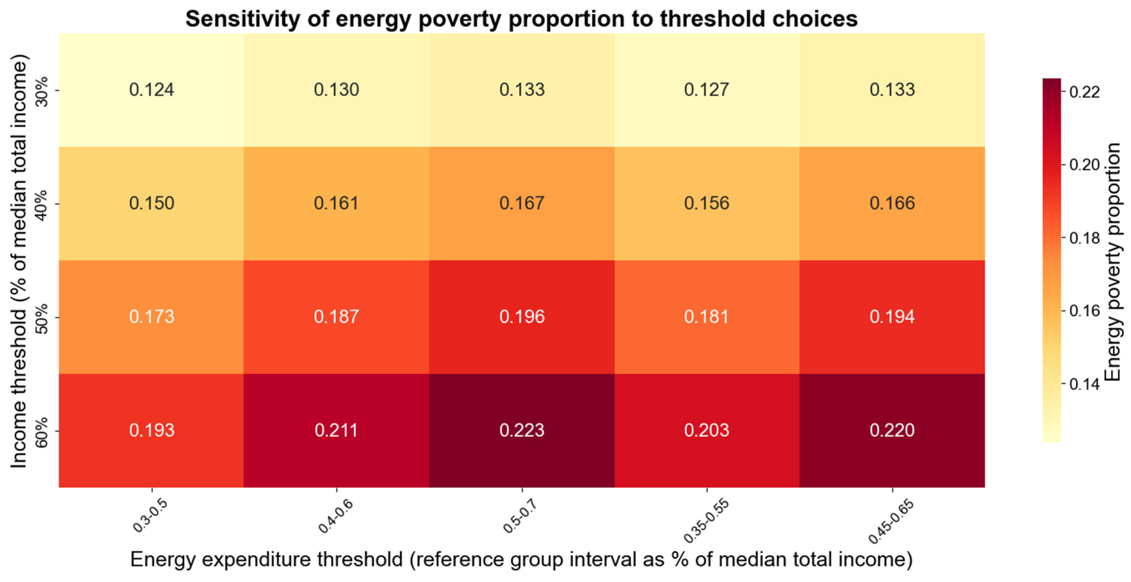
The heatmap clearly illustrates how the proportion of people experiencing energy poverty varies across combinations of income and energy expenditure thresholds. This indicates that the absolute proportion of energy poverty fluctuates between the range of 12.4% and 22.3% depending on the benchmark threshold. Whereas the relative pattern of the proportion of energy poverty rising monotonically as the income threshold increases remains consistent. Moreover, the revenue threshold is the primary factor determining the scale of identification, whereas adjustments to the energy expenditure range result in only minor fluctuations. Therefore, the test of robustness confirms the internal logical consistency of the two-dimensional identification framework developed for this study. While demonstrating that the key findings influencing the identification of energy poverty are not dependent on the choice of specific thresholds, this also indicates that our model exhibits good robustness and reliability.
Based on data from the six periods between 2012 and 2022, we used data obtained from the National Bureau of Statistics of China encompassing the annual rural absolute poverty lines. The annual per capita poverty line for each year was 2625, 2800, 2952, 2995, 3442, and 4000 yuan. Absolute poverty is defined as a household’s per capita disposable income below the poverty line for the corresponding year. The results are depicted in Table A3:
Table A3.
Comparison with the absolute poverty line.
Table A3 indicates that the energy poverty identification method employed in this study exhibits a high degree of consistency in relation to the traditional absolute poverty line. A total of 16,176 household samples, representing 91.2% of the total sample of 17,731 households, were classified as ‘energy-poor/non-energy-poor’ using the LIHC framework—a classification that coincided with the ‘absolute poverty/non-absolute poverty’ classification based on income. The Cohen’s Kappa coefficient of 0.669 indicates a moderate level of agreement between the two. Among the 17,731 households surveyed, 1562 were identified as being in both energy poverty and absolute poverty, whereas 1294 households were identified as being in energy poverty but not in absolute poverty. Thus, their income was slightly above the absolute poverty line, but they were still within energy poverty levels due to the heavy burden of energy costs. Notably, 261 households living in absolute poverty were not identified as energy-poor, since their energy consumption was either low or accruing to a beneficial status of receiving subsidies. Interestingly, when energy poverty captures the dual predicament of ‘low income combined with a high energy burden’, it differs from income poverty despite being highly correlated with it. Hence, the Kappa coefficient confirms the validity and robustness of the classification.
Table A4.
Classification Performance Comparison between Different Models.
Model 1 comprises two core variables: net income and energy expenditure. On the test set, its overall F1 score was 93%, whereas the accuracy, recall, and F1 scores for each risk category ranged between 89% and 97%. This demonstrates robust classification performance and good generalisation ability. Therefore, the model can also serve as a reference model in practical applications, offering both interpretability and reliability.
Similarly, Model 2 achieved near-perfect classification results on the test set: the overall F1 score reached 100%, whereas the precision, recall, and F1 scores for each risk category ranged between 0.99 and 1.00. This result is primarily attributable to the data characteristic attributes, such as when some of the categorical variables included in Model 2 exhibit a high degree of consistency with the defining variables of the risk categories. Consequently, the performance of Model 2 should be interpreted as a theoretical upper bound for performance, reflecting the structural consistency between the classification criteria and input variables.
For the reasons outlined above, the results of Model 2 outlined in this study are not treated as the primary basis for assessing the model’s validity; hence, they are not used to support any policy implications or empirical conclusions. Their inherent value, therefore, lies primarily in verifying the internal consistency of the entire variable system as well as providing a reference for the upper limit of prediction that future research can focus on to achieve robust results under conditions of full disclosure.
References
- Frederick S. Pardee Institute for International Futures (Josef Korbel School of International Studies, University of Denver); United Nations Development Programme (UNDP)). Advancing the SDG Push with Equitable Low-Carbon Pathways; UNDP Flagship Publication No. 4; Frederick S. Pardee Institute for International Futures (Josef Korbel School of International Studies, University of Denver): Denver, CO, USA; United Nations Development Programme (UNDP): New York, NY, USA, 2024; pp. 1–29. Available online: https://www.undp.org/publications/advancing-sdg-push-equitable-low-carbon-pathways (accessed on 10 March 2025).
- International Energy Agency. Tracking SDG7: The Energy Progress Report 2024; International Energy Agency: Paris, France, 2024; Available online: https://documents.worldbank.org/en/publication/documents-reports/documentdetail/099031225175211404 (accessed on 2 January 2025).
- Antunes, M.; Teotónio, C.; Quintal, C.; Martins, R. Energy Affordability Across and Within 26 European Countries: Insights into the Prevalence and Depth of Problems Using Microeconomic Data. Energy Econ. 2023, 127, 107044. [Google Scholar] [CrossRef] [Scilit]
- Addai, B.; Tang, W.; Twumasi, M.A.; Asante, D.; Agyeman, A.S. Access to Financial Services and Lighting Energy Consumption: Empirical Evidence from Rural Ghana. Energy 2022, 253, 124109. [Google Scholar] [CrossRef] [Scilit]
- Hills, J. Getting the Measure of Fuel Poverty: Final Report of the Fuel Poverty Review; 1465-3001; LSE Research Online: London, UK, 2012; Available online: https://eprints.lse.ac.uk/43153 (accessed on 6 December 2024).
- Semple, T.; Rodrigues, L.; Harvey, J.; Figueredo, G.; Gillott, M. A Critical Review of Existing Fuel Poverty Definitions in England: Problematisation, Obfuscation and Compatibility with a Just Energy Transition. Energy Res. Soc. Sci. 2025, 127, 104263. [Google Scholar] [CrossRef] [Scilit]
- Papada, L.; Kaliampakos, D. Artificial Neural Networks as a Tool to Understand Complex Energy Poverty Relationships: The Case of Greece. Energies 2024, 17, 3163. [Google Scholar] [CrossRef] [Scilit]
- Lesala, M.E.; Mukumba, P.; KeChrist, O. Rural Energy Poverty: An Investigation into Socioeconomic Drivers and Implications for Off-Grid Households in the Eastern Cape Province, South Africa. Economies 2025, 13, 128. [Google Scholar] [CrossRef] [Scilit]
- Wang, F.; Zha, D.; Geng, H.; Zhang, C. Regional Disparities and Spatial Convergence in Energy Poverty: Evidence from China’s Rural Areas. Environ. Dev. Sustain. 2025, 1–31. [Google Scholar] [CrossRef]
- Chen, F.; Qiu, H.; Yang, S. Energy Transition of the Poor: Quasi-Experimental Evidence from Poverty Alleviation Relocation Program in China. Energy Policy 2025, 199, 114536. [Google Scholar] [CrossRef] [Scilit]
- Kashour, M.; Jaber, M.M. Revisiting Energy Poverty Measurement for the European Union. Energy Res. Soc. Sci. 2024, 109, 103420. [Google Scholar] [CrossRef] [Scilit]
- Boardman, B. Opportunities and Constraints Posed by Fuel Poverty on Policies to Reduce the Greenhouse Effect in Britain. Appl. Energy 1993, 44, 185–195. [Google Scholar] [CrossRef] [Scilit]
- Sy, S.A.; Mokaddem, L. Energy Poverty in Developing Countries: A Review of the Concept and Its Measurements. Energy Res. Soc. Sci. 2022, 89, 102562. [Google Scholar] [CrossRef] [Scilit]
- Bouzarovski, S.; Damigos, D.; Kmetty, Z.; Simcock, N.; Robinson, C.; Jayyousi, M.; Crowther, A. Energy Justice Intermediaries: Living Labs in the Low-Carbon Transformation. Local Environ. 2023, 28, 1534–1551. [Google Scholar] [CrossRef] [Scilit]
- Nussbaumer, P.; Bazilian, M.; Modi, V. Measuring Energy Poverty: Focusing on What Matters. Renew. Sustain. Energy Rev. 2012, 16, 231–243. [Google Scholar] [CrossRef] [Scilit]
- Khanna, R.A.; Li, Y.; Mhaisalkar, S.; Kumar, M.; Liang, L.J. Comprehensive Energy Poverty Index: Measuring Energy Poverty and Identifying Micro-Level Solutions in South and Southeast Asia. Energy Policy 2019, 132, 379–391. [Google Scholar] [CrossRef] [Scilit]
- Al Kez, D.; Foley, A.; Lowans, C.; Del Rio, D.F. Energy Poverty Assessment: Indicators and Implications for Developing and Developed Countries. Energy Convers. Manag. 2024, 307, 118324. [Google Scholar] [CrossRef] [Scilit]
- Li, Y.; Zhang, W.; Zhao, B.; Sharp, B.; Nie, J. Does Energy Poverty Affect Subjective Well-Being? Evidence from a Cross-Country Analysis. Appl. Econ. 2026, 58, 141–156. [Google Scholar] [CrossRef] [Scilit]
- Igawa, M.; Managi, S. Energy Poverty and Income Inequality: An Economic Analysis of 37 Countries. Appl. Energy 2022, 306, 118076. [Google Scholar] [CrossRef] [Scilit]
- Hosan, S.; Sen, K.K.; Rahman, M.M.; Karmaker, S.C.; Chapman, A.J.; Saha, B.B. Mitigating Energy Poverty: A Panel Analysis of Energy Policy Interventions in Emerging Economies of the Asia-Pacific Region. Energy 2024, 291, 130367. [Google Scholar] [CrossRef] [Scilit]
- Simcock, N.; Jenkins, K.E.H.; Lacey-Barnacle, M.; Martiskainen, M.; Mattioli, G.; Hopkins, D. Identifying Double Energy Vulnerability: A Systematic and Narrative Review of Groups At-Risk of Energy and Transport Poverty in the Global North. Energy Res. Soc. Sci. 2021, 82, 102351. [Google Scholar] [CrossRef] [Scilit]
- Śmiech, S.; Karpinska, L.; Bouzarovski, S. Impact of Energy Transitions on Energy Poverty in the European Union. Renew. Sustain. Energy Rev. 2025, 211, 115311. [Google Scholar] [CrossRef] [Scilit]
- Homsy, G.C.; Kang, K.E. Energy Burden: Exploring the Intersection of Race, Income, and Community Characteristics Across the United States. Energy Res. Soc. Sci. 2025, 127, 104207. [Google Scholar] [CrossRef] [Scilit]
- Waldron, R.; Sugrue, S.; Simcock, N.; Holloway, L. Precarious Lives: Exploring the Intersection of Insecure Housing and Energy Conditions in Ireland. Energy Res. Soc. Sci. 2025, 121, 103992. [Google Scholar] [CrossRef] [Scilit]
- del Río, P.; Burguillo, M.; Kiefer, C.P. Which Are the Main Determinants of Energy Poverty? A Systematic Review of the Literature. Energy Effic. 2025, 18, 58. [Google Scholar] [CrossRef] [Scilit]
- Yue, J.; Chen, S.; Weng, Z.; Xie, Y.; Xu, M. Heterogeneous Characteristics of Household Energy Poverty and Sustainable Development: Perspective from the Household Life Cycle. Energy 2025, 337, 138581. [Google Scholar] [CrossRef] [Scilit]
- Tang, L.; Mahmood, H.; Khalid, S. Examining the Impact of Structural Reforms on Energy Poverty: A Threshold Effect of Energy Affordability. Energy 2025, 320, 135101. [Google Scholar] [CrossRef] [Scilit]
- Vandyck, T.; Della Valle, N.; Temursho, U.; Weitzel, M. EU Climate Action Through an Energy Poverty Lens. Sci. Rep. 2023, 13, 6040. [Google Scholar] [CrossRef] [Scilit] [PubMed]
- Spandagos, C.; Reaños, M.A.T.; Lynch, M.Á. Energy Poverty Prediction and Effective Targeting for Just Transitions with Machine Learning. Energy Econ. 2023, 128, 107131. [Google Scholar] [CrossRef] [Scilit]
- Dalla Longa, F.; Sweerts, B.; van der Zwaan, B. Exploring the Complex Origins of Energy Poverty in The Netherlands with Machine Learning. Energy Policy 2021, 156, 112373. [Google Scholar] [CrossRef] [Scilit]
- Burlig, F.; Knittel, C.; Rapson, D.; Reguant, M.; Wolfram, C. Machine Learning from Schools About Energy Efficiency. J. Assoc. Environ. Resour. Econ. 2020, 7, 1181–1217. [Google Scholar] [CrossRef] [Scilit]
- Gawusu, S.; Jamatutu, S.A.; Zhang, X.; Moomin, S.T.; Ahmed, A.; Mensah, R.A.; Das, O.; Ackah, I. Spatial Analysis and Predictive Modeling of Energy Poverty: Insights for Policy Implementation. Environ. Dev. Sustain. 2026, 28, 851–898. [Google Scholar] [CrossRef] [Scilit]
- Gawusu, S.; Jamatutu, S.A.; Ahmed, A. Predictive Modeling of Energy Poverty with Machine Learning Ensembles: Strategic Insights from Socioeconomic Determinants for Effective Policy Implementation. Int. J. Energy Res. 2024, 2024, 9411326. [Google Scholar] [CrossRef] [Scilit]
- Kim, H.; Kwon, Y.; Choi, Y. Determinants of Electricity Consumption of Energy-Vulnerable Group Using Ensemble Gradient-Boosting Algorithm. KSCE J. Civ. Eng. 2022, 26, 5010–5021. [Google Scholar] [CrossRef] [Scilit]
- Zou, W.; Cheng, X.; Fan, Z.; Lin, C. Measuring and Decomposing Relative Poverty in China. Land 2023, 12, 316. [Google Scholar] [CrossRef] [Scilit]
- Ravallion, M. On Measuring Global Poverty. Annu. Rev. Econ. 2020, 12, 167–188. [Google Scholar] [CrossRef] [Scilit]
- Darvas, Z. Why Is It So Hard to Reach the EU’s Poverty Target? Soc. Indic. Res. 2019, 141, 1081–1105. [Google Scholar] [CrossRef] [Scilit]
- Popova, D. Impact of Equity in Social Protection Spending on Income Poverty and Inequality. Soc. Indic. Res. 2023, 169, 697–721. [Google Scholar] [CrossRef] [Scilit]
- Patel, J.A.; Nielsen, F.B.H.; Badiani, A.A.; Assi, S.; Unadkat, V.; Patel, B.; Ravindrane, R.; Wardle, H. Poverty, Inequality and COVID-19: The Forgotten Vulnerable. Public Health 2020, 183, 110. [Google Scholar] [CrossRef] [Scilit]
- Sovacool, B.K. Defining, Measuring, and Tackling Energy Poverty. Energy Poverty Glob. Chall. Local Solut. 2014, 2, 21–53. [Google Scholar] [CrossRef] [Scilit]
- Siksnelyte-Butkiene, I.; Streimikiene, D.; Lekavicius, V.; Balezentis, T. Energy Poverty Indicators: A Systematic Literature Review and Comprehensive Analysis of Integrity. Sustain. Cities Soc. 2021, 67, 102756. [Google Scholar] [CrossRef] [Scilit]
- Anastasiou, A.; Zaroutieri, E. Energy Poverty and the Convergence Hypothesis Across EU Member States. Energy Effic. 2023, 16, 38. [Google Scholar] [CrossRef] [Scilit]
- Sarkodie, S.A.; Strezov, V. Empirical Study of the Environmental Kuznets Curve and Environmental Sustainability Curve Hypothesis for Australia, China, Ghana and USA. J. Clean. Prod. 2018, 201, 98–110. [Google Scholar] [CrossRef] [Scilit]
- Zheng, J.; Dang, Y.; Assad, U. Household Energy Consumption, Energy Efficiency, and Household Income–Evidence from China. Appl. Energy 2024, 353, 122074. [Google Scholar] [CrossRef] [Scilit]
- Ackermann, I.; Radulescu, D. Unveiling the Energy Price Tag-Assessing the Burden of Household Energy Expenditures Among European Countries. Energy Policy 2026, 208, 114919. [Google Scholar] [CrossRef] [Scilit]
- Choumert-Nkolo, J.; le Roux, L. Leaving the Hearth You Know: Internal Migration and Energy Poverty. World Dev. 2024, 180, 106628. [Google Scholar] [CrossRef] [Scilit]
- Burlinson, A.; Giulietti, M.; Law, C.; Liu, H.-H. Fuel Poverty and Financial Distress. Energy Econ. 2021, 102, 105464. [Google Scholar] [CrossRef] [Scilit] [PubMed]
- Sultana, N.; Hossain, S.Z.; Almuhaini, S.H.; Düştegör, D. Bayesian Optimization Algorithm-Based Statistical and Machine Learning Approaches for Forecasting Short-Term Electricity Demand. Energies 2022, 15, 3425. [Google Scholar] [CrossRef] [Scilit]
- Lundberg, S.M.; Erion, G.; Chen, H.; DeGrave, A.; Prutkin, J.M.; Nair, B.; Katz, R.; Himmelfarb, J.; Bansal, N.; Lee, S.-I. From Local Explanations to Global Understanding with Explainable AI for Trees. Nat. Mach. Intell. 2020, 2, 56–67. [Google Scholar] [CrossRef] [Scilit] [PubMed]
- Aas, K.; Jullum, M.; Løland, A. Explaining Individual Predictions When Features Are Dependent: More Accurate Approximations to Shapley Values. Artif. Intell. 2021, 298, 103502. [Google Scholar] [CrossRef] [Scilit]
- Piao, X.; Managi, S. Household Energy-Saving Behavior, Its Consumption, and Life Satisfaction in 37 Countries. Sci. Rep. 2023, 13, 1382. [Google Scholar] [CrossRef] [Scilit]
- Zhu, M. Unveiling Complexities: Income Inequality and Inequality of Opportunity in China. Rev. Dev. Econ. 2025, 29, 670–717. [Google Scholar] [CrossRef] [Scilit]
- Ceglia, F.; Marrasso, E.; Samanta, S.; Sasso, M. Addressing Energy Poverty in the Energy Community: Assessment of Energy, Environmental, Economic, and Social Benefits for an Italian Residential Case Study. Sustainability 2022, 14, 15077. [Google Scholar] [CrossRef] [Scilit]
- Tu, G.; Morrissey, K.; Sharpe, R.A.; Taylor, T. Combining Self-Reported and Sensor Data to Explore the Relationship Between Fuel Poverty and Health Well-Being in UK Social Housing. Wellbeing Space Soc. 2022, 3, 100070. [Google Scholar] [CrossRef] [Scilit]
- Hao, N.; Peng, B.; Tang, K.; Wu, J. Does Energy Poverty Trap Exist in Chinese Cities? Evidence from Evaluating the Co-Evolution of Energy Consumption and Income. Cities 2024, 150, 105082. [Google Scholar] [CrossRef] [Scilit]
- Yang, H.; Li, X.; Yan, J. The Impact of Energy Poverty on Subjective Well-Being: Evidence from China. Humanit. Soc. Sci. Commun. 2025, 12, 379. [Google Scholar] [CrossRef] [Scilit]
- Mustre-del-Río, J.; Sánchez, J.M.; Mather, R.; Athreya, K. The Effects of Macroeconomic Shocks: Household Financial Distress Matters. Rev. Financ. Stud. 2025, 38, 564–604. [Google Scholar] [CrossRef] [Scilit]
- Nsenkyire, E.; Nunoo, J.; Sebu, J.; Iledare, O. Household Multidimensional Energy Poverty: Impact on Health, Education, and Cognitive Skills of Children in Ghana. Child. Indic. Res. 2023, 16, 293–315. [Google Scholar] [CrossRef] [Scilit]
- Middlemiss, L. Who Is Vulnerable to Energy Poverty in the Global North, and What Is Their Experience? Wiley Interdiscip. Rev. Energy Environ. 2022, 11, e455. [Google Scholar] [CrossRef] [Scilit]
- Qi, X.; Chen, J.; Wang, J.; Liu, H.; Ding, B. The Impact of Urbanization on the Alleviation of Energy Poverty: Evidence from China. Cities 2024, 151, 105130. [Google Scholar] [CrossRef] [Scilit]
- Adjei-Mantey, K.; Inglesi-Lotz, R.; Amoah, A. Environmental Consciousness and Household Energy Poverty in Ghana. Glob. Environ. Change 2024, 88, 102896. [Google Scholar] [CrossRef] [Scilit]
- Shi, H.; Li, S.; Zhang, J. The Impact of Water Scarcity on Energy Poverty and Its Mechanism: Evidence from a Rural Household Analysis in Northern China. Water Policy 2025, 27, 615–638. [Google Scholar] [CrossRef] [Scilit]
- Burguillo, M.; del Río, P.; Juez-Martel, P. Does Energy Poverty Influence Decarbonisation Through Electrification of the Heating Sector? Energy Build. 2024, 312, 114110. [Google Scholar] [CrossRef] [Scilit]
- Lu, S.; Ren, J. A Global Spatial–Temporal Energy Poverty Assessment and Social Impacts Analysis. Int. J. Energy Res. 2024, 2024, 8247272. [Google Scholar] [CrossRef] [Scilit]
- Cervantes, M.Á.M.; Solís, L.R. Energy Poverty and Social Justice in Mexico: The Rights of Electricity Consumers. Electr. J. 2024, 37, 107372. [Google Scholar] [CrossRef] [Scilit]
- Karpinska, L.; Śmiech, S. Multiple Faces of Poverty. Exploring Housing-Costs-Induced Energy Poverty in Central and Eastern Europe. Energy Res. Soc. Sci. 2023, 105, 103273. [Google Scholar] [CrossRef] [Scilit]
- Zalostiba, D.; Kiselovs, D. A review: The Energy Poverty Issue in the European Union and Latvia. Latv. J. Phys. Tech. Sci. 2021, 58, 227–248. [Google Scholar] [CrossRef] [Scilit]
- Gao, Z.; Jia, Z.; Zhang, C.; Gao, S.; Yang, X.; Hao, Y. Energy Poverty in China: Measurement, Regional Inequality, and Dynamic Evolution. Energies 2026, 19, 143. [Google Scholar] [CrossRef] [Scilit]
- Wang, Y.; Xu, B. Assessing the Effective Drivers of Energy Poverty Reduction in China: A Spatial Perspective. Energy 2025, 320, 135427. [Google Scholar] [CrossRef] [Scilit]
- Lu, C.; Wan, S. Determinants of Energy Poverty Among Chinese Households: Risk Prediction Model Using Machine Learning Algorithms. Energy 2025, 337, 138502. [Google Scholar] [CrossRef] [Scilit]
- Feng, J.; Chen, Y.; Gulzar, F.; Mirzaliev, S.; Alofaysan, H.; Mark, P. The Dynamics of Energy Poverty in China: Household Level Analysis and Mitigation Strategies. Energy Sci. Eng. 2025, 13, 2011–2021. [Google Scholar] [CrossRef] [Scilit]
- Apergis, N.; Polemis, M.; Soursou, S.-E. Energy Poverty and Education: Fresh Evidence from a Panel of Developing Countries. Energy Econ. 2022, 106, 105430. [Google Scholar] [CrossRef] [Scilit]
- Martiskainen, M.; Sovacool, B.K.; Lacey-Barnacle, M.; Hopkins, D.; Jenkins, K.E.; Simcock, N.; Mattioli, G.; Bouzarovski, S. New Dimensions of Vulnerability to Energy and Transport Poverty. Joule 2021, 5, 3–7. [Google Scholar] [CrossRef] [Scilit]
- Matschoss, K.; Laakso, S.; Rinkinen, J. Disruptions and Energy Demand: How Finnish Households Responded to the Energy Crisis of 2022. Energy Res. Soc. Sci. 2025, 121, 103977. [Google Scholar] [CrossRef] [Scilit]
- Bardazzi, R.; Gastaldi, F.; Iafrate, F.; Pansini, R.V.; Pazienza, M.G.; Pollastri, C. Inflation and Distributional Impacts: Have Mitigation Policies Been Successful for Vulnerable and Energy Poor Households? Energy Policy 2024, 188, 114082. [Google Scholar] [CrossRef] [Scilit]
- Banna, H.; Alam, A.; Chen, X.H.; Alam, A.W. Energy Security and Economic Stability: The Role of Inflation and War. Energy Econ. 2023, 126, 106949. [Google Scholar] [CrossRef] [Scilit]
- Lambin, X.; Schleich, J.; Faure, C. The Energy Efficiency Gap in the Rental Housing Market: It Takes Both Sides to Build a Bridge. Energy J. 2023, 44, 75–92. [Google Scholar] [CrossRef] [Scilit]
- Haider, S.; Mahapatra, B.; Mohammad, S.; Mitra, A. Understanding the Socioeconomic Determinants of Cooking Fuel Expenditure in Uttar Pradesh, India. Discov. Sustain. 2024, 5, 182. [Google Scholar] [CrossRef] [Scilit]
- Das, I.; Rogers, B.; Nepal, M.; Jeuland, M. Fuel Stacking Implications for Willingness to Pay for Cooking Fuels in Peri-Urban Kathmandu Valley, Nepal. Energy Sustain. Dev. 2022, 70, 482–496. [Google Scholar] [CrossRef] [Scilit]
- Jiang, K.; Xing, R.; Luo, Z.; Li, Y.; Wang, J.; Zhang, W.; Zhu, Y.; Men, Y.; Shen, G.; Tao, S. Unclean but Affordable Solid Fuels Effectively Sustained Household Energy Equity. Nat. Commun. 2024, 15, 9761. [Google Scholar] [CrossRef] [Scilit]
- Eisfeld, K.; Seebauer, S. The Energy Austerity Pitfall: Linking Hidden Energy Poverty with Self-Restriction in Household Use in Austria. Energy Res. Soc. Sci. 2022, 84, 102427. [Google Scholar] [CrossRef] [Scilit]
- Zambrano-Monserrate, M.A. Mapping the Impact of Artificial Intelligence on Energy Poverty: New Evidence from Spatial Panel Models. Energy Econ. 2025, 151, 108909. [Google Scholar] [CrossRef] [Scilit]
- Hussain, S.A.; Razi, F.; Hewage, K.; Sadiq, R. The Perspective of Energy Poverty and 1st Energy Crisis of Green Transition. Energy 2023, 275, 127487. [Google Scholar] [CrossRef] [Scilit]
- Della Valle, N.; Maduta, C.; D’Agostino, D.; Koukoufikis, G. Unpacking Energy Vulnerability in the European Union: Linking Thermal Discomfort with Adaptive Capacity. Energy Res. Soc. Sci. 2025, 129, 104376. [Google Scholar] [CrossRef] [Scilit]
- Großmann, K.; Oettel, H.; Sandmann, L. At the Intersection of Housing, Energy, and Mobility Poverty: Trapped in Social Exclusion. Energies 2024, 17, 1925. [Google Scholar] [CrossRef] [Scilit]
- Waldron, R.; Sugrue, S.; Wijburg, G.; Manzo, L.K. The ‘Double Precarity’of Housing and Energy Conditions: Lived Experiences and Structural Drivers. Energy Res. Soc. Sci. 2025, 129, 104373. [Google Scholar] [CrossRef] [Scilit]
- Drago, C.; Gatto, A. Measuring Energy Poverty and Energy Vulnerability. Sustain. Cities Soc. 2023, 92, 104450. [Google Scholar] [CrossRef] [Scilit]
- Wang, Y.; Lin, B. Can Energy Poverty Be Alleviated by Targeting the Low Income? Constructing a Multidimensional Energy Poverty Index in China. Appl. Energy 2022, 321, 119374. [Google Scholar] [CrossRef] [Scilit]
- Mei, X.; Seo, B.K. The Relationships Among Housing, Energy Poverty, and Health: A Scoping Review. Energy Sustain. Dev. 2024, 83, 101568. [Google Scholar] [CrossRef] [Scilit]
- Zhao, J.; Dong, K.; Dong, X.; Shahbaz, M. How Renewable Energy Alleviate Energy Poverty? A Global Analysis. Renew. Energy 2022, 186, 299–311. [Google Scholar] [CrossRef] [Scilit]
- besnİLİ memİŞ, O.; Aydin, R. Indirect Impact of Public Expenditures and Inflation on Energy Poverty: Empirical Evidence from 32 Developing Countries. Appl. Econ. 2025, 57, 805–822. [Google Scholar] [CrossRef] [Scilit]
- Rakotomena, M.; Ricci, O. Measuring Energy Poverty: A Climate-Aware Multidimensional Approach. Soc. Indic. Res. 2025, 180, 943–969. [Google Scholar] [CrossRef] [Scilit]
- Prakash, K.; Churchill, S.A.; Smyth, R. Perception and Reality of Energy Poverty in Australia: Do They Shape Voting Intentions? Aust. Econ. Rev. 2025, 58, 131–139. [Google Scholar] [CrossRef] [Scilit]
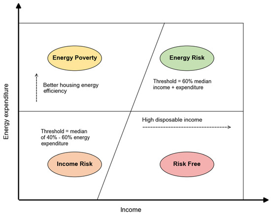
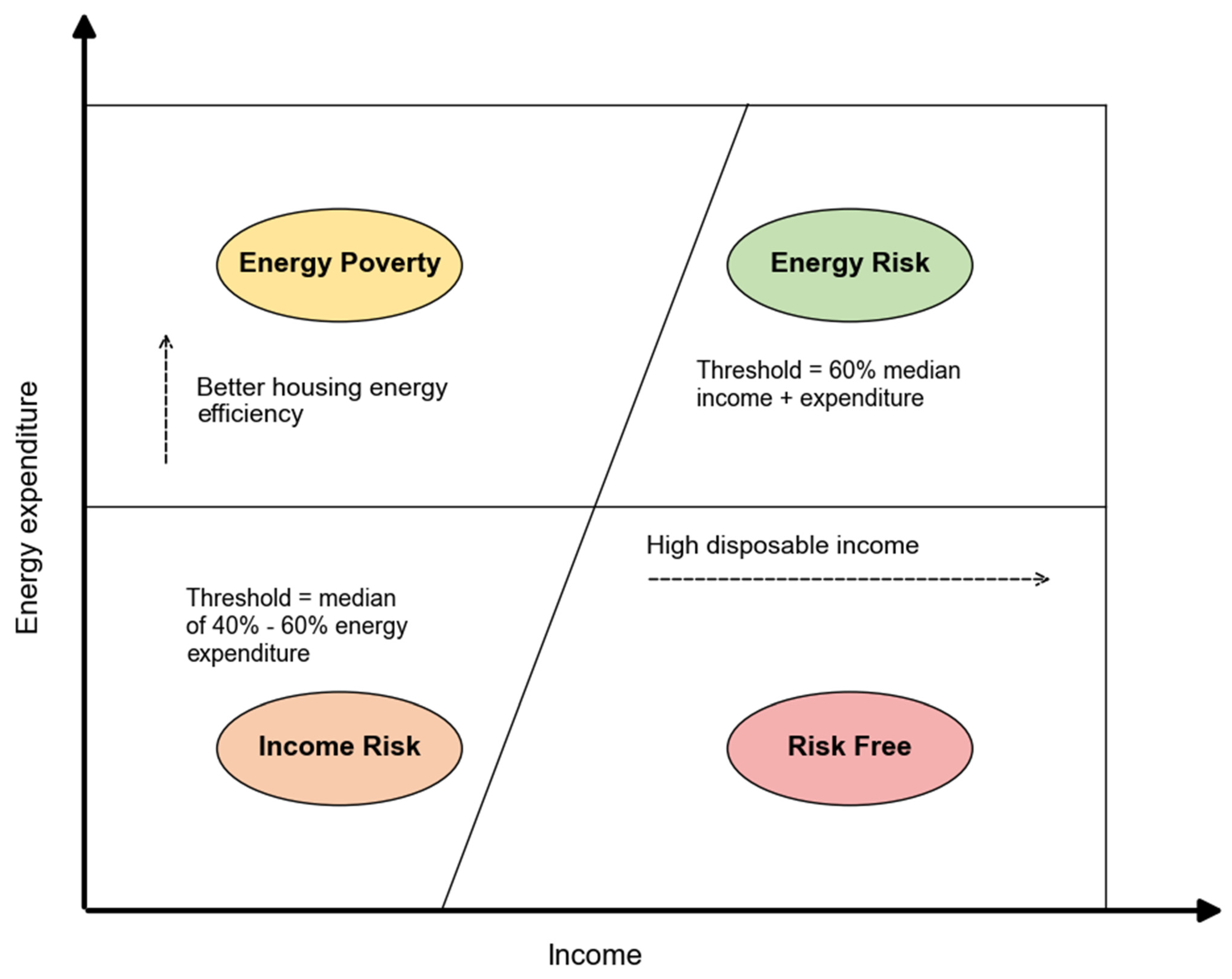
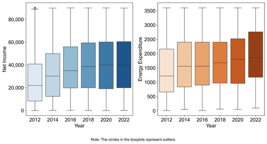
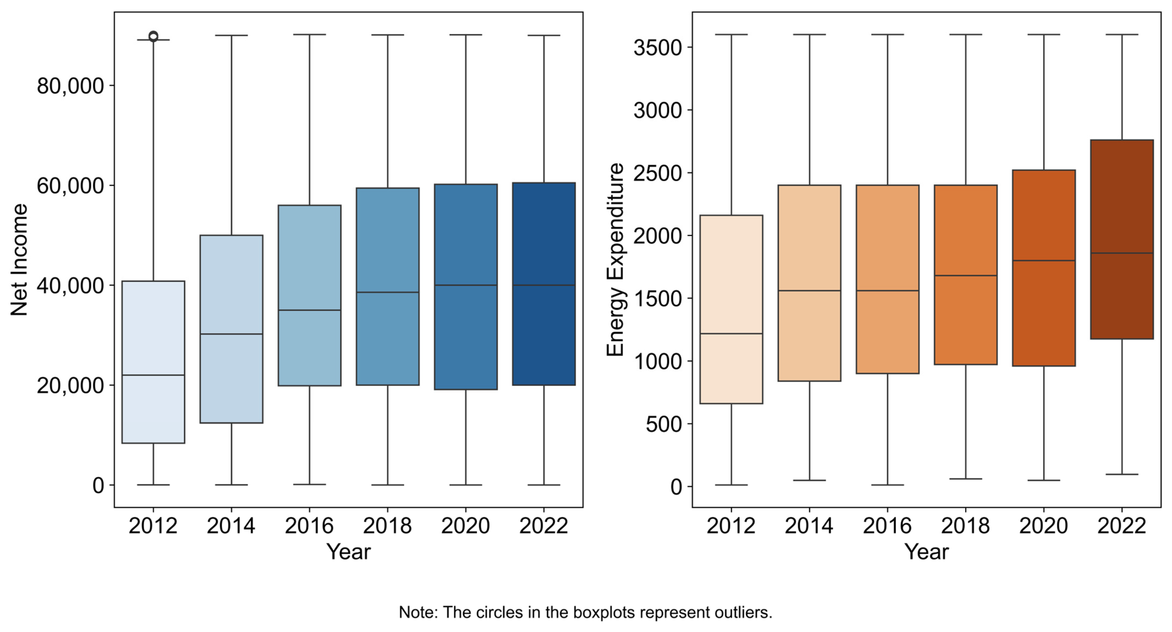
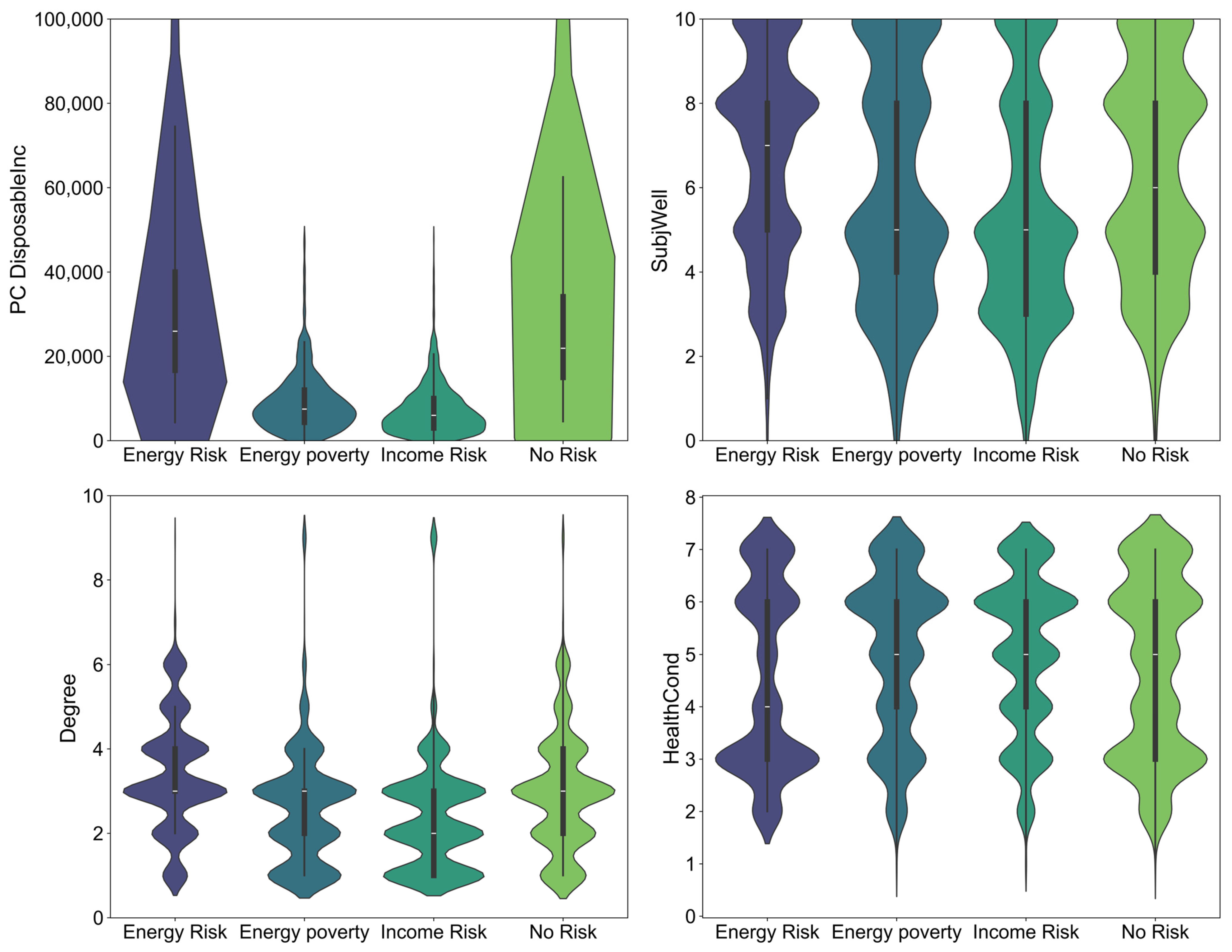
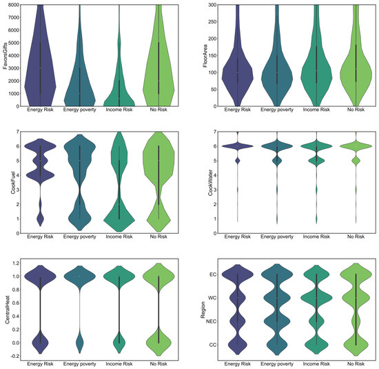
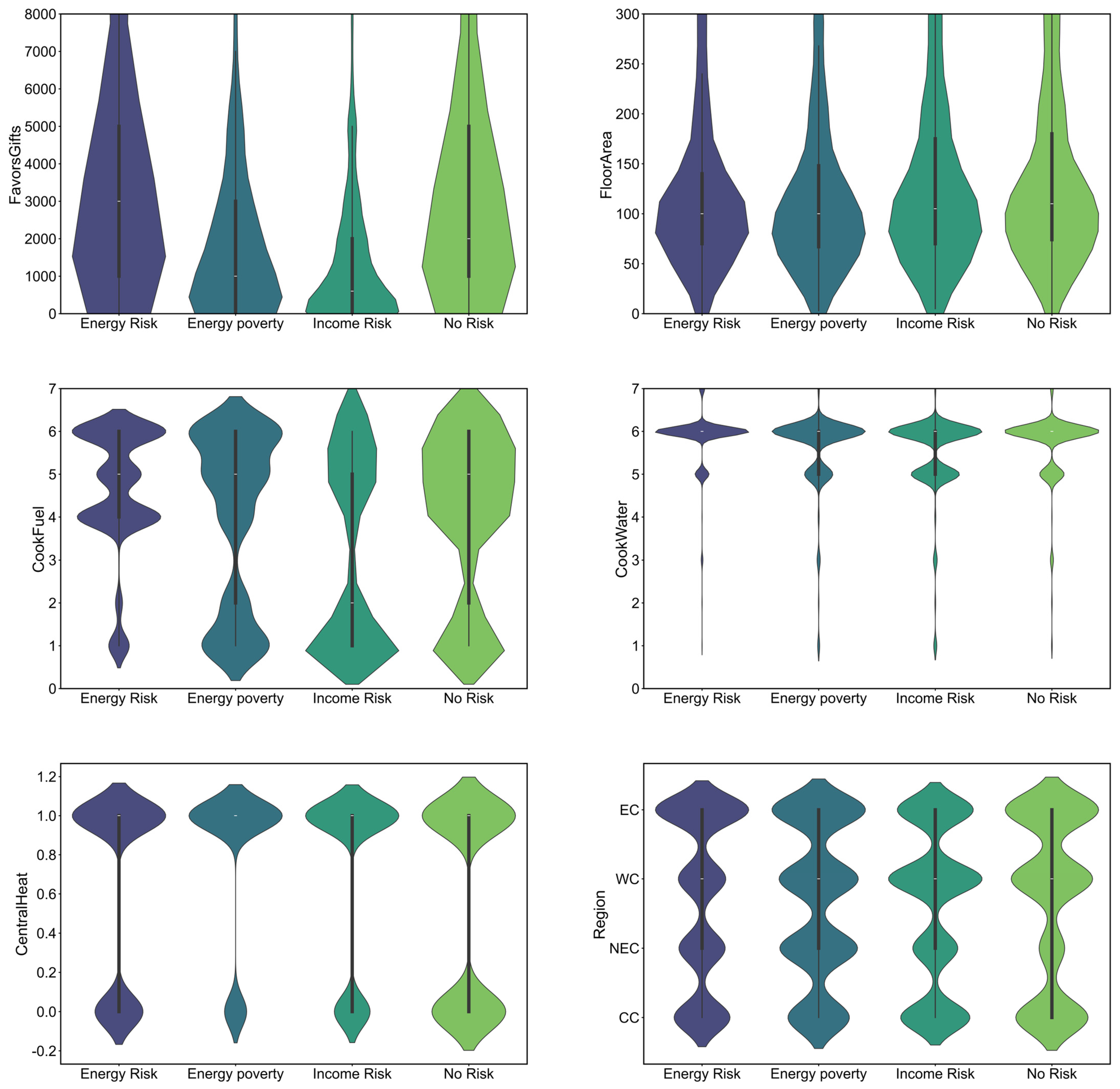
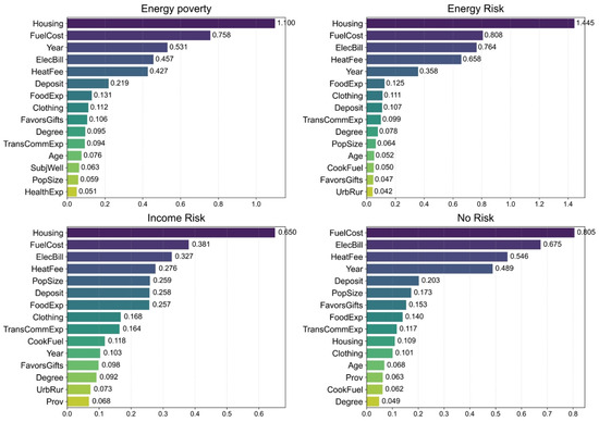
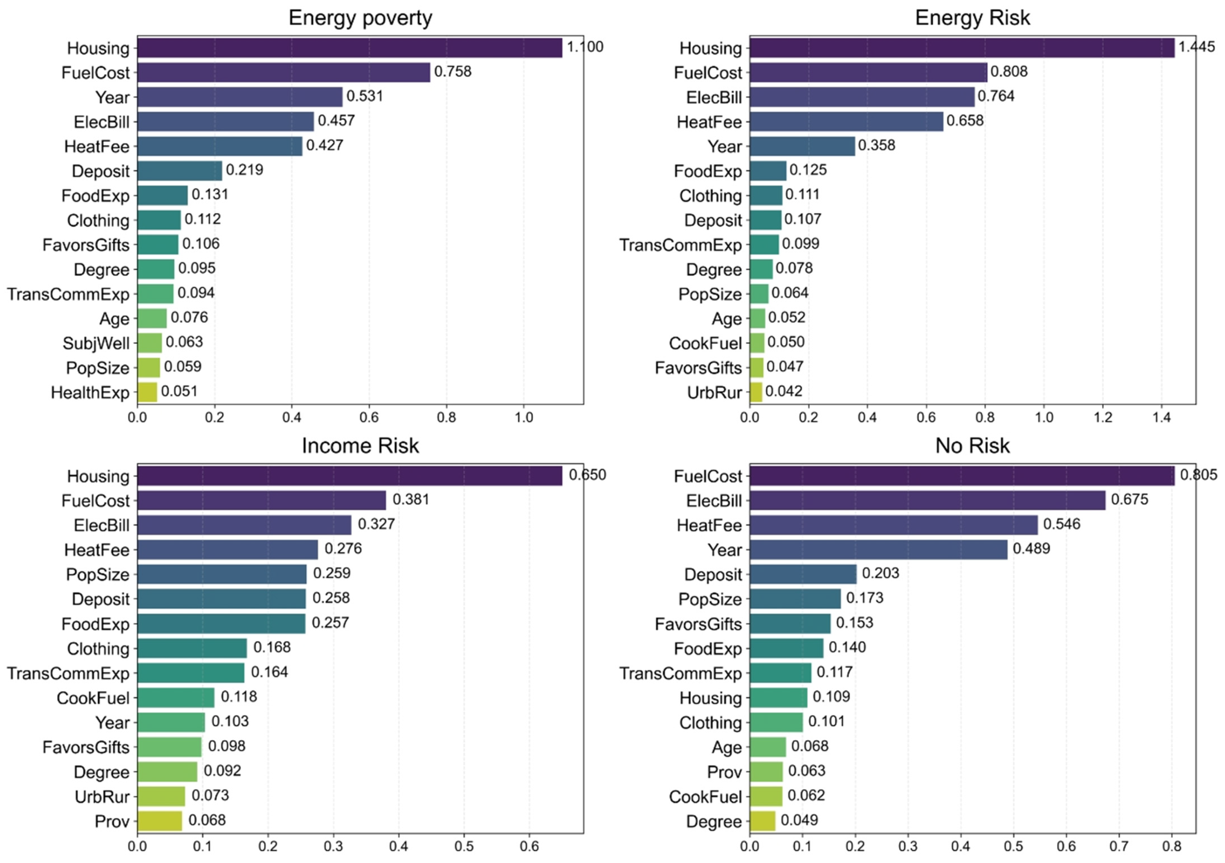
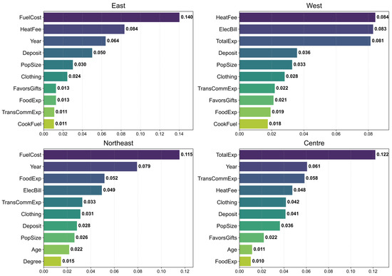
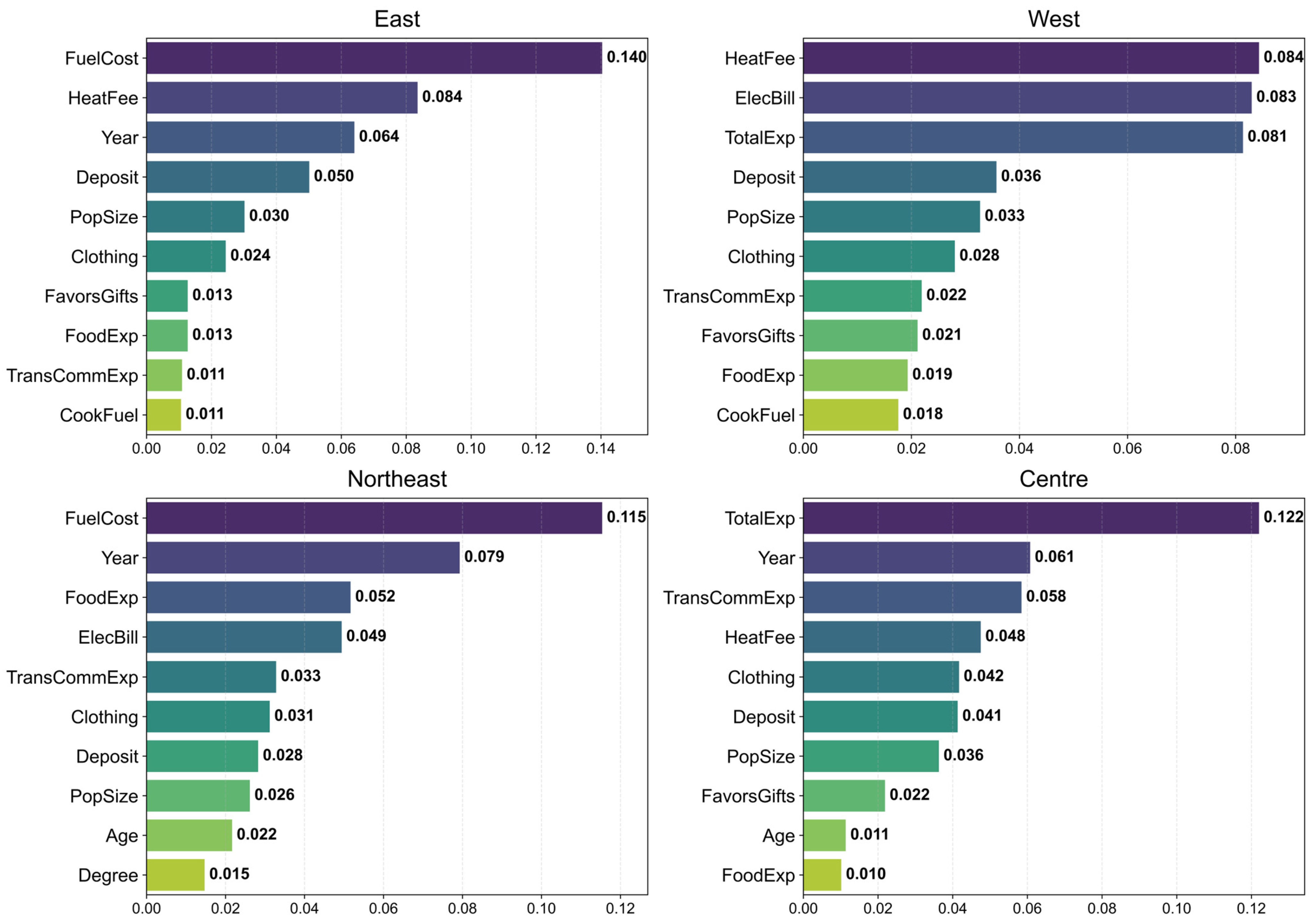
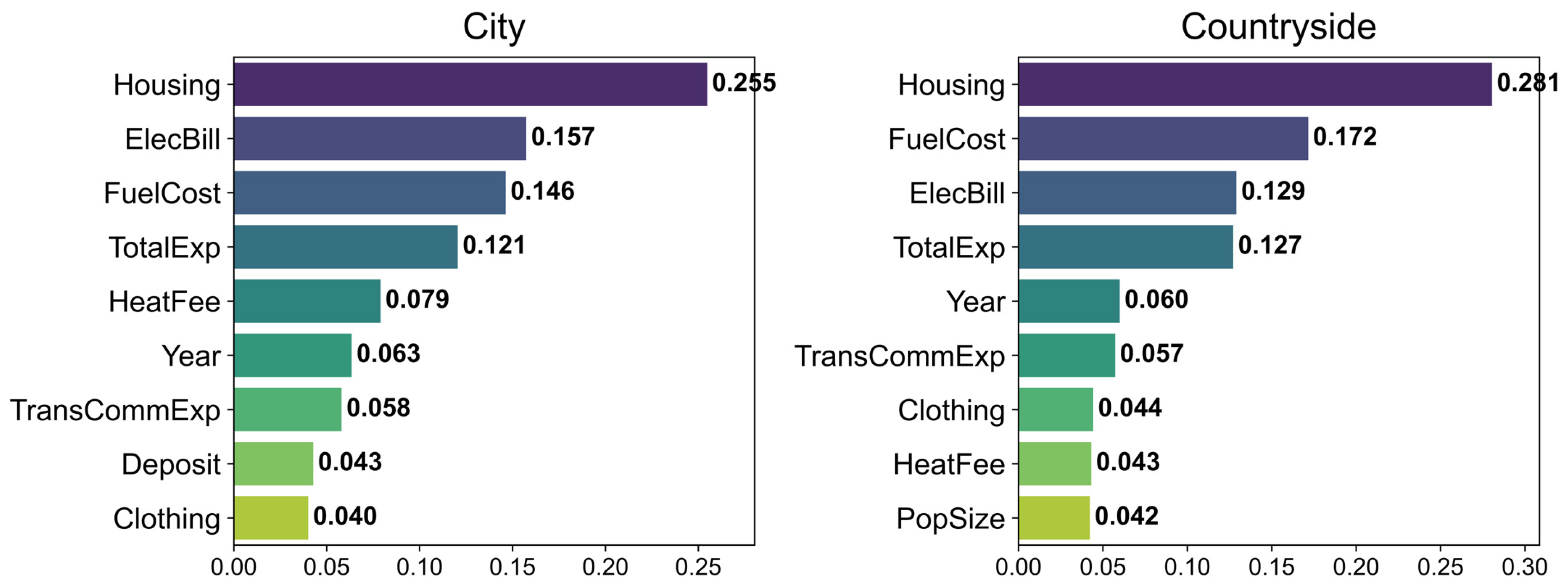
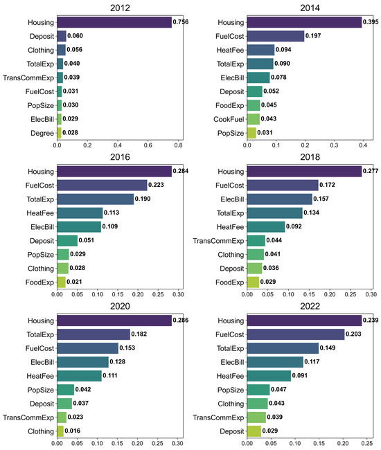
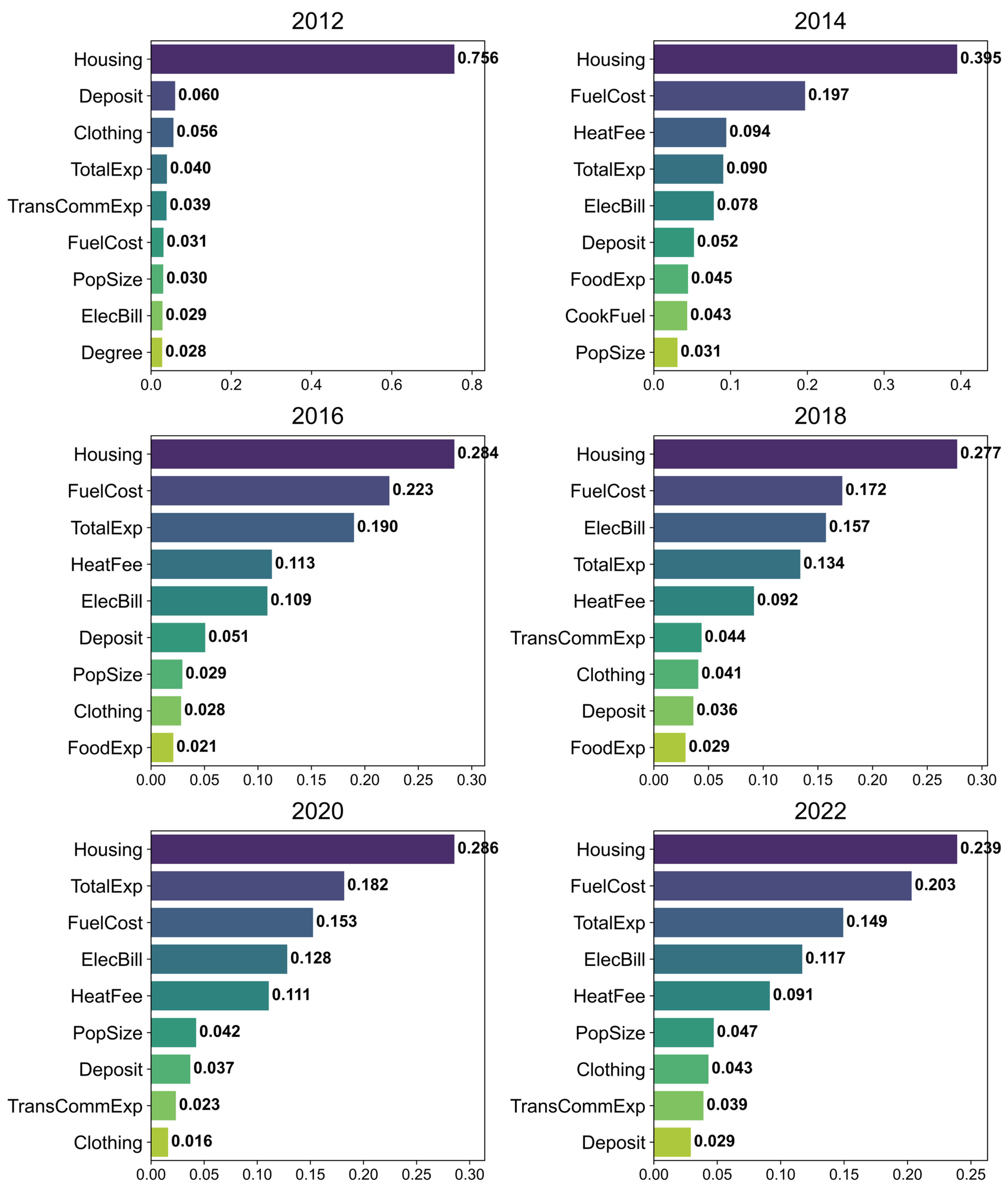
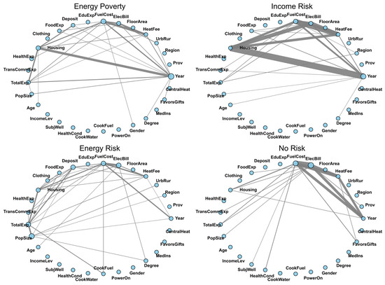
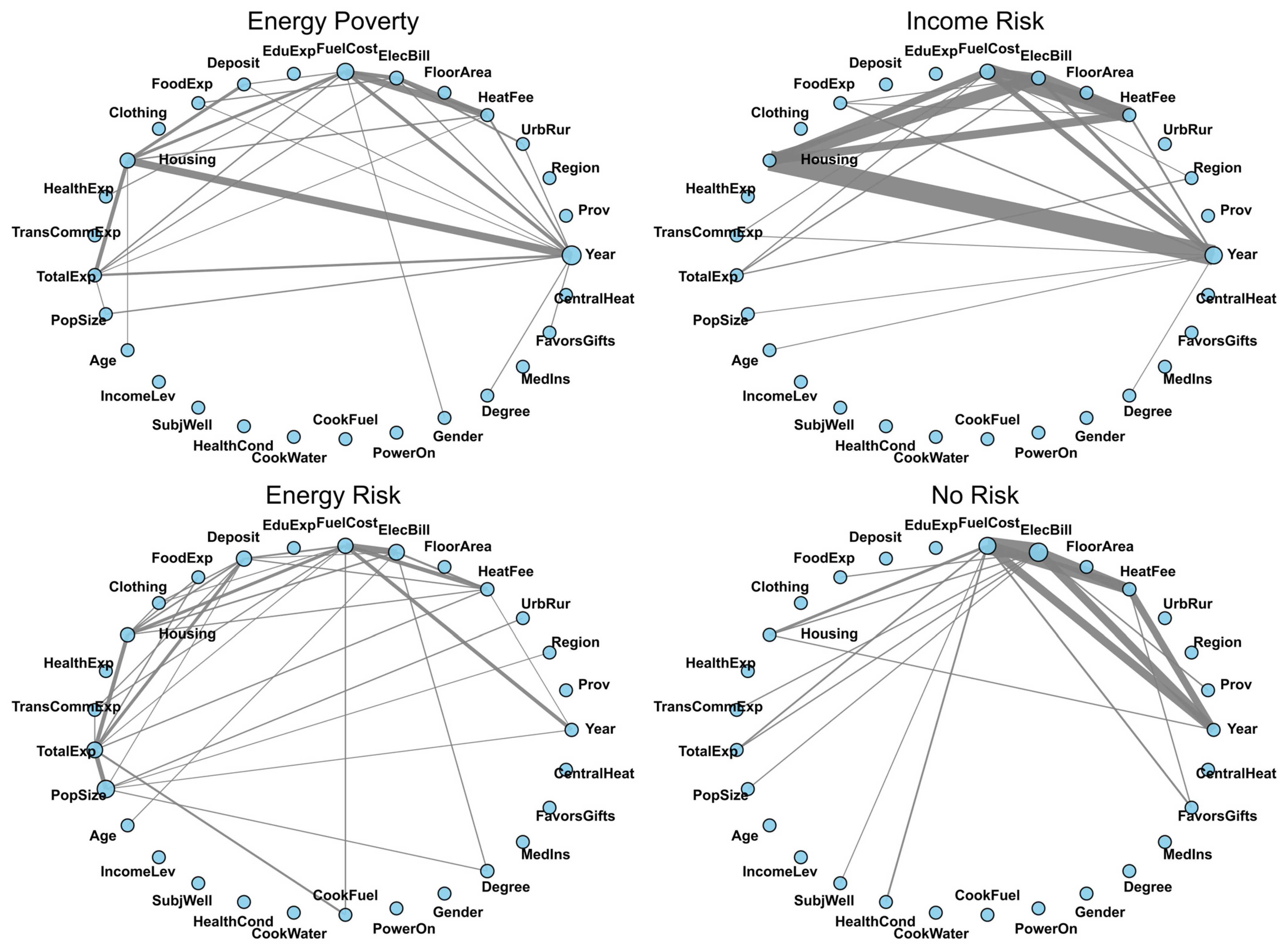
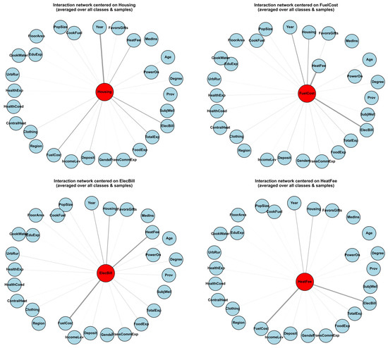
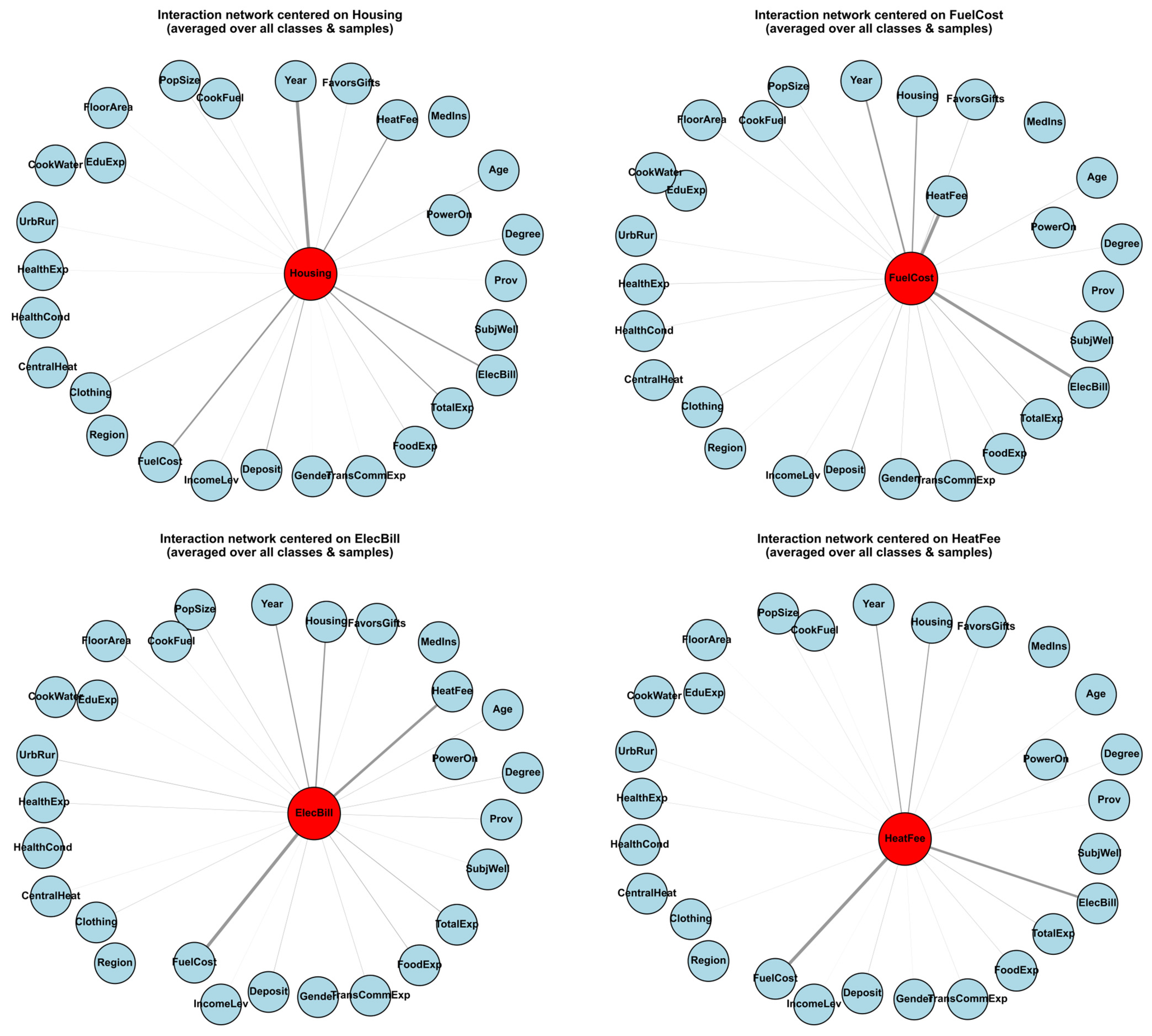
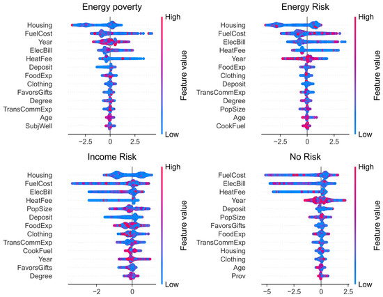
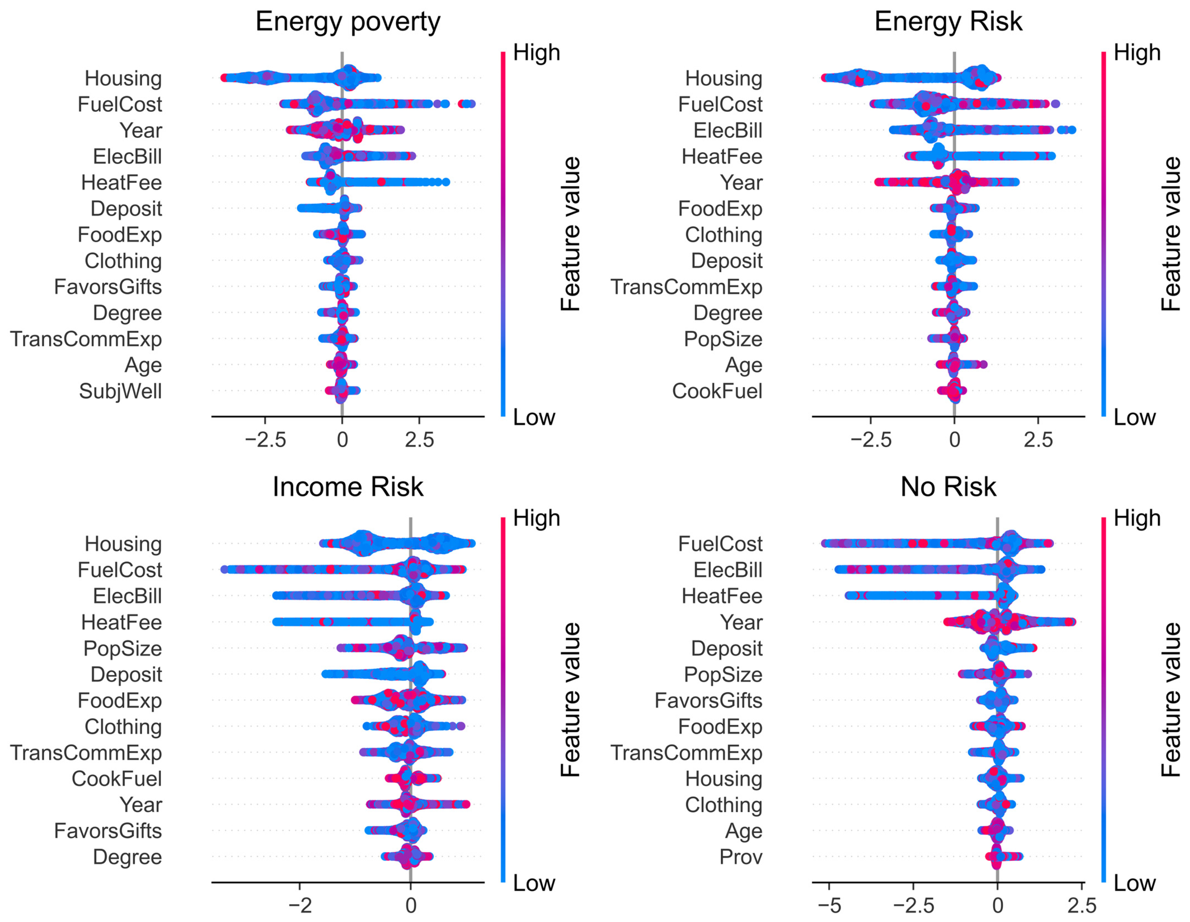
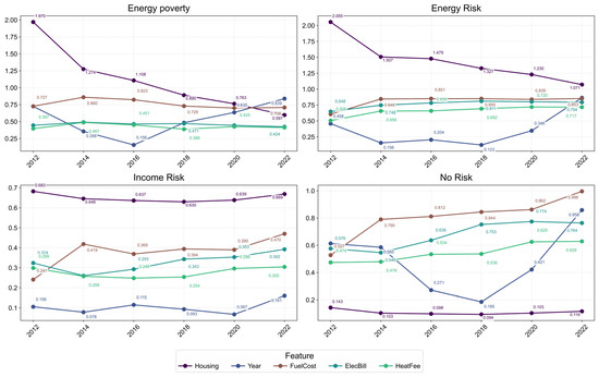
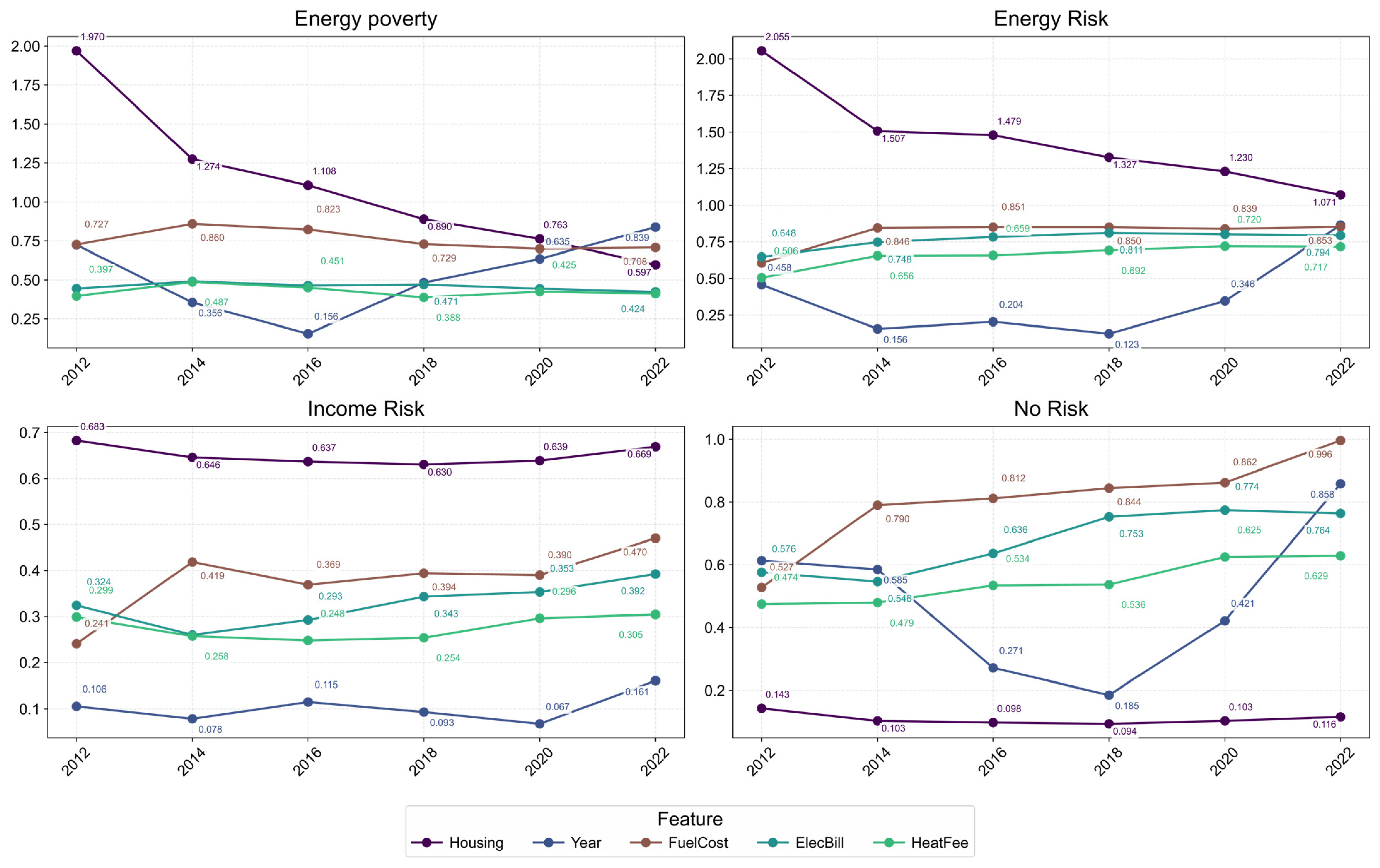
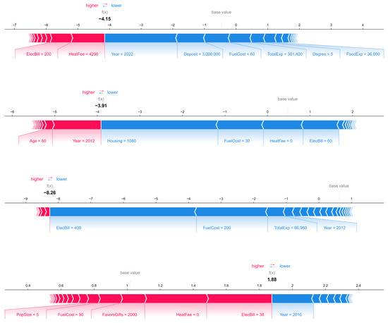
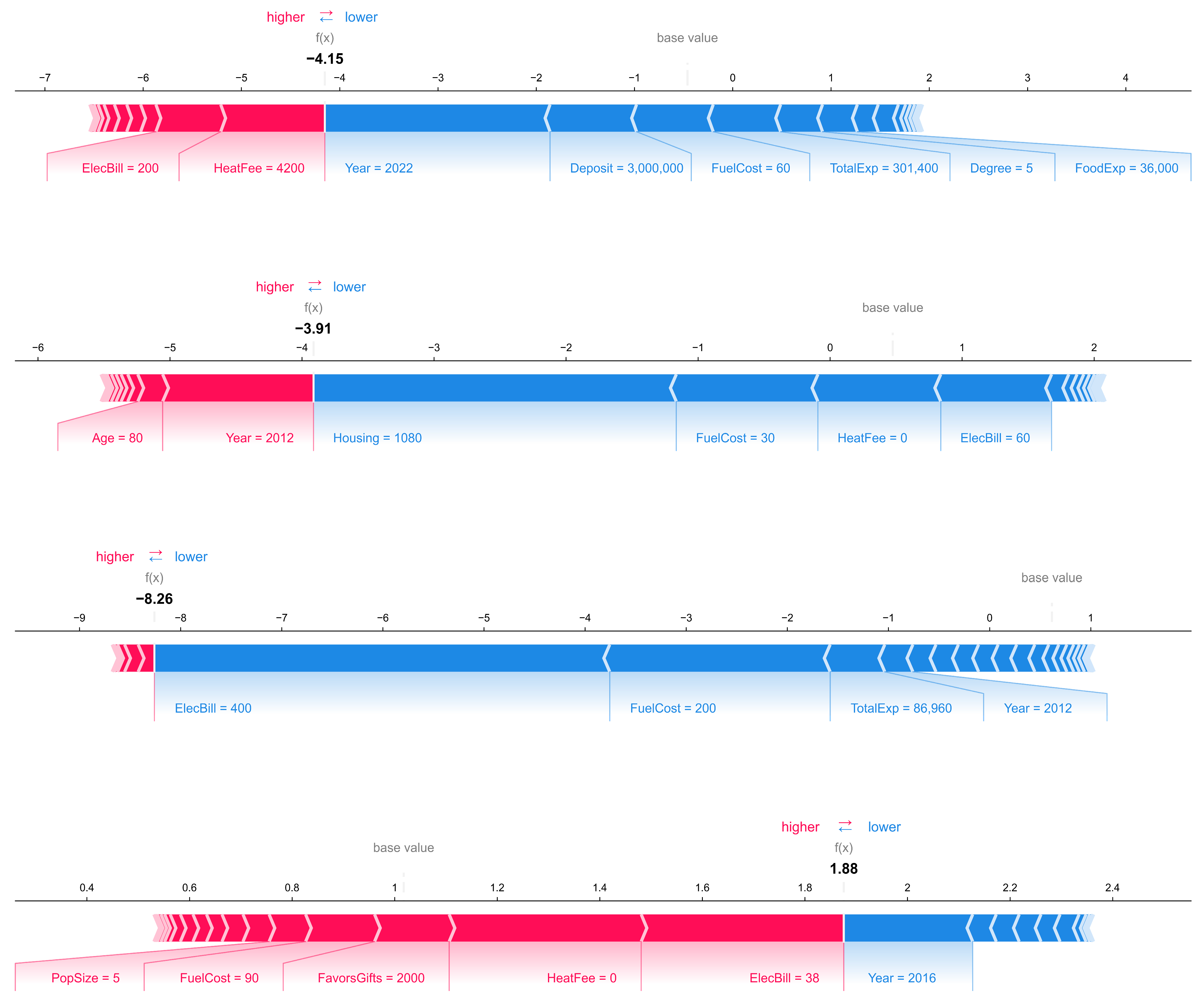

Disclaimer/Publisher’s Note: The statements, opinions and data contained in all publications are solely those of the individual author(s) and contributor(s) and not of MDPI and/or the editor(s). MDPI and/or the editor(s) disclaim responsibility for any injury to people or property resulting from any ideas, methods, instructions or products referred to in the content. |
© 2026 by the authors. Licensee MDPI, Basel, Switzerland. This article is an open access article distributed under the terms and conditions of the Creative Commons Attribution (CC BY) license.