Shadow Size Distribution Analysis for Automated Classification of Wood Chip Particle Size Distribution Under Bulk Conditions

Abstract

Italy is one of Europe’s largest consumers of wood pellets, while domestic production remains comparatively limited. In parallel, wood chips (WC) represent a strategic biofuel for power generation, where particle size distribution (PSD) affects handling and storage. Conventional PSD assessment relies on time-consuming methodology. This study proposes a patent-pending image-processing approach (Shadow Size Distribution—SSD analysis) for PSD classification of WC under bulk conditions. One hundred samples were characterized via both standard analysis and SSD. PSD data were aggregated into fine and coarse macro-fractions and used to define binary class labels. Multivariate analyses (PERMANOVA, PCA) and Support Vector Classifier (SVC) models were employed to evaluate the discriminative capability of SSD features. PCA revealed coherent relationships between PSD macro-variables and key shadow descriptors, particularly shadow number and area. The best SVC configuration achieved 0.77 test accuracy, with strong recall for coarse samples. Although overall performance was constrained by dataset size and imbalance, the results demonstrate that SSD features retain meaningful granulometric information, supporting further development toward automated, in-line PSD monitoring systems. From a sustainability perspective, the proposed SSD-based approach enables faster and potentially in-line monitoring of biomass quality, supporting more efficient combustion processes, reduced emissions, and improved resource management in bioenergy systems.

1. Introduction

Italy is among the leading European consumers of wood pellets for residential use [1]. Between 2015 and 2024, Italy imported an average of approximately 2.067 thousand tonnes of wood pellets per year, accounting for about 29% of total European imports, which averaged roughly 7.232 thousand tonnes annually over the same period [2]. However, national production does not fully match consumption levels [3,4].

In recent years, the average annual wood pellet production in Europe amounted to approximately 17.170 thousand tonnes. Within this context, Germany, Austria, and Estonia recorded average outputs of 2.884, 1.439, and 1.428 thousand tonnes, respectively. In contrast, Italy achieved an average production of about 396 thousand tonnes, corresponding to roughly 2.3% of total European production over the same period [2]. This discrepancy may partly be explained by the comparatively high costs associated with pellet production and plant maintenance [5,6].

Consequently, several studies have begun investigating the use of Wood Chips (WC) and mini-WC as an alternative to pellets for residential stoves, focusing on their energetic efficiency, emissions, and potential cost advantages [7,8]. However, the Italian context currently lacks a robust network of production facilities or suppliers for mini-WC, as producers still face limited market demand for large-scale operations [8].

Expanding the scope beyond domestic applications, the utilization of WC for energy production constitutes a key strategic element for many European countries [9,10]. In Italy, numerous thermoelectric power plants are fueled by WC and other types of solid biomass, whose number has increased in recent years [11,12].

For the economic and environmental sustainability of woody biomass, it is critical that the biomass exhibits high-quality characteristics [13]. Such quality is influenced by multiple parameters, including nitrogen content, ash content, and moisture content, which directly impact combustion efficiency, greenhouse gas emissions, and the propensity for equipment corrosion [14,15].

ISO 17225-9 [16] establishes the physical and chemical parameters with which WC must comply in order to be classified as a high-quality industrial material. Among the parameters considered by the standard, calorific value, and ash content are among the most extensively monitored and studied, both in research contexts and in quality control activities. However, the standard considers an additional aspect that is often overlooked: Particle Size Distribution (PSD) [15,17,18].

The PSD of WC derives from multiple interacting factors, including the type of chipper and its cutting mechanism (disc or drum), the wood species and its moisture condition, the characteristics of the incoming feedstock (e.g., whole logs versus branches), and the operational productivity or working speed of the chipping process [19].

PSD also affects several operational aspects, including the material’s flowing properties during automated handling [20], therefore directly affecting boiler feeding efficiency [21]. It also affects logistical aspects related to transporting materials beyond forest harvesting sites and the aeration and fermentation dynamics of WC stockpiles [22,23]. PSD may also directly or indirectly affect combustion efficiency, and consequently on emission levels [24]. For instance, the length of wood pellets directly affects combustion efficiency as it can lead to more or less irregular fuel bed formation, creating air pockets that affect combustion kinetics [25,26,27]. Therefore, a similar effect can reasonably be expected in WC as the PSD varies.

The PSD of solid biofuels is typically determined using standardised sieve analysis procedures such as ISO 17827-1 [28], which are based on the mechanical separation of a representative sample into size classes using calibrated sieves. The resulting mass distribution across size fractions provides a quantitative description of fuel heterogeneity and is widely used to classify biomass fuels and assess their handling and combustion behavior. However, this methodology is relatively time-consuming and may be affected by operator-dependent variability.

Consequently, numerous studies have investigated the use of alternative methodologies for assessing PSD. For instance, Febbi et al. [29,30] investigated the application of image-processing techniques for the clusterization of WC fractions into distinct PSD-clusters. Gil et al. [31] adopted a comparable methodology to assess the PSD of WC and corn stalks, focusing however on more limited particle size fractions (0.1–5 mm).

Although previous studies have applied image-processing techniques, the analysed particles generally need to remain static during image acquisition. Conversely, Hartmann et al. [32] and Labati et al. [33] proposed dynamic approaches in which the PSD of WC is assessed during free fall. Although these techniques have varying degrees of accuracy, they share one key limitation that makes them difficult to apply in industrial contexts: the need for the particles to be clearly separated [29,30,31,32]. Such limitations make it difficult to integrate these techniques into automated systems for directly measuring PSD within industrial biomass combustion processes. In thermoelectric power plants, biomass is handled and stored in bulk hindering the clear separation of particles required by conventional image processing measurement methods. In this context, improving the monitoring and control of biomass quality parameters such as PSD is essential not only for process optimization but also for enhancing the environmental and economic sustainability of bioenergy supply chains.

This study presents a novel patent-pending image-processing method for the size classification of WC under stacked or bulk conditions. The approach, previously validated for the dimensional classification of wood pellets under bulk conditions [27,34], addresses the limitations of ISO-based and conventional image analysis techniques by enabling dimensional characterization without the need for isolated particles. The methodology, hereinafter referred to as Shadow Size Distribution (SSD) analysis, is based on the correlation between particle size and the geometric features of shadows generated under controlled lateral illumination. Although this paper does not apply the methodology in an industrial setting, the minimal hardware requirements make it inherently suitable for in-line deployment. This enables the methodology to be extended beyond controlled laboratory conditions and applied effectively in dynamic, real-world operating environments. Thus, by enabling real-time or near-real-time assessment of biomass characteristics under bulk conditions, the proposed methodology contributes to the development of more sustainable energy systems through improved efficiency, reduced waste, and enhanced process control.

2. Materials & Methods

This section provides a detailed description of the materials used and methodological approach employed in the study. The workflow includes sample collection and preparation, conventional PSD analysis, SSD analysis, preliminary and advanced statistical analyses, and the development, tuning, and validation of PSD classification models.

2.1. Sample Preparation and Conventional Analysis

A total of 100 WC samples, each weighing approximately 2.5 kg, were collected directly from thermoelectric power plants located throughout Italy. In accordance with standard ISO 14780 [35], each sample was homogenized and reduced by quartering to obtain 100 representative subsamples, each weighing approximately 500 g. These subsamples were then stabilized and subjected to PSD analysis using the method described in ISO 17827 [28].

PSD analysis was performed using an AS400 sieve shaker (Retsch, Haan, Germany) equipped with standard sieves (63, 45, 31.5, 16, 8, and 3.15 mm) arranged in descending order, with a collection pan for fines (<3.15 mm). In the subsequent text, commas will be omitted for the sake of brevity; thus, 3.15 and 31.5 will become 3 and 31, respectively. The analysis was carried out in accordance with ISO 17827-1, which requires samples to be conditioned to a moisture content below 20% prior to sieving. According to the standard procedure, particles longer than 100 mm were first separated and weighed. The remaining sample was then placed in the sieve stack and sieved for 15 min at 170 rpm, with the rotation direction reversed after 7 min.

After sieving, the material retained on each sieve and in the collection pan is recovered and weighed using a precision balance. The PSD is expressed as the mass percentage of each size fraction relative to the total sample mass. After each analysis, the sample was recovered and subjected to SSD analysis [27,34].

2.2. Shadow Size Distribution Analysis

The SSD methodology builds upon a previously developed prototypal imaging system designed to characterize bulk samples through the analysis of shadow patterns generated under controlled illumination. This approach was first introduced and thoroughly described in the paper that initially proposed and applied it [34]. For a detailed explanation, the reader is referred to the cited literature. For completeness, a brief overview is provided here, and a concise description of the system is included in the appendix (Appendix A).

The system comprises a dark room housing a sample tray and a Raspberry Pi 4B computational unit and a Raspberry Pi camera. The dark room minimizes external light interference and ensures reproducible imaging conditions, while the sample is leveled on the tray prior to acquisition.

Images are captured and processed using software developed in Python and based on the OpenCV library [36]. The processing pipeline automatically binarizes the acquired images to remove the foreground and isolate the shadows produced by the interaction between incident light and the sample. From the segmented shadows, the software extracts a set of quantitative descriptors (SSD-based features), including the number of detected shadows and statistical, geometric, and morphological features related to their size and shape (

Table 1. SSD-based features extracted from the acquired images after segmentation. The reported descriptors include quantitative parameters related to the number of detected shadows, as well as their geometric and morphological properties.

Shadow-Based Features	Tag	Description	Mathematical Description
Number of Shadows	$N_{os}$	Number of objects or shadows detected in the image.	-
Average dimension of Shadows	$Are{a}_{PX}$	Average size (in pixels) of the shadows.	${\displaystyle \frac{1}{n}}{\displaystyle {\displaystyle \sum }_{i=1}^n}Are{a}_i$
Eccentricity	-	Measures the average elongation of the shadows; a value of 0 indicates a circular shape, while higher values signify greater elongation.	$\sqrt{1-{\displaystyle \frac{{\left(\mathrm{Minor} \mathrm{Axis} \mathrm{Length}\right)}^2}{{\left(\mathrm{Major} \mathrm{Axis} \mathrm{Length}\right)}^2}}}$
Solidity	-	The average ratio of pixels in the detected shadows to the pixels in their convex hull, indicating the compactness of the objects.	${\displaystyle \frac{Contour Area}{Convex Hull Area}}$
Entropy	-	A quantitative measure of noisiness in the image; high entropy indicates a complex mix of black and white pixels, while low entropy suggests a simpler, less varied composition.	$-{\displaystyle {\displaystyle \sum }_{i=0}^1}{p}_i{\log }_2\left(p_i\right)$
Extent	-	The average ratio of pixels in the shadows to the total number of pixels in their bounding boxes, providing a measure of the objects’ coverage within their bounding regions.	${\displaystyle \frac{Object Area}{Bounding Rectangle Area}}$

). These SSD-based features are automatically stored in a structured dataset for subsequent analysis.

In the original system configuration, multiple illumination angles were tested to evaluate their influence on shadow formation. In the present study, only the upper-light source was used, as it provided the best performance in the previous work. Apart from this modification, the hardware setup, acquisition procedure, and image-processing workflow remain consistent with those previously described.

2.3. Preliminary Statistical Analysis and Label Generation

Descriptive statistical analysis was used to explore the dataset, and its main characteristics were visualised using scatter plots, box plots, and a heatmap to identify underlying patterns and trends. To support the development of subsequent classification models, the PSD variables were pre-processed by aggregating the data from each sieve into two macro-features. Specifically, the PSD features were grouped into a fine fraction, representing the sum of components associated with particle sizes below 16 mm (Equation (1)), and a coarse fraction, representing the sum of components associated with sizes above 16 mm (Equation (2)). This threshold was selected in accordance with the standard classification of woody biomass (ISO 17827-1, Table 1) [37].

An intermediate fraction was initially considered; however, due to the limited dataset size, a three-class subdivision would have resulted in unbalanced and statistically weak groups, and was therefore not adopted.

A ratio between the coarse and fine fractions was then defined (Equation (3)) to quantify their relative predominance. To ensure a robust threshold estimation, extreme high values in the ratio distribution were identified using an interquartile range (IQR)-based criterion (upper fence) and excluded solely for the computation of the threshold. The median of the filtered distribution was then used as a data-driven threshold. This threshold was subsequently applied to classify all samples: those with a ratio lower than the median were labelled as belonging to the fine class, while those with a ratio equal to or greater than the median were assigned to the coarse class (Equation (4)). This approach provided a compact and informative feature representation while ensuring a balanced and statistically robust categorisation of the dataset for the subsequent classification stage. From this point onward, the raw PSD features corresponding to individual sieve fractions were discarded, and the analysis was conducted exclusively on the aggregated macro-features defined by Equations (1) and (2):

$$F_{\mathrm{fine}}={\displaystyle \sum }_{i\in f}PS{D}_i,\hspace{1em}f=\{<3, 3–8, 8–16\}$$

(1)

$$F_{\mathrm{coarse}}={\displaystyle \sum }_{i\in c}PS{D}_i,\hspace{1em}c=\{16–31, 31–45, 45–63, 63–100,>100\}$$

(2)

$$R={\displaystyle \frac{F_{\mathrm{coarse}}}{F_{\mathrm{fine}}}}$$

(3)

$$\begin{array}{c}Class Label=\left\{\begin{array}{cc}PS{D}_{fine},& R<\mathrm{median}\left(R_{\mathrm{clean}}\right)\\ PS{D}_{coarse},& R\ge \mathrm{median}\left(R_{\mathrm{clean}}\right)\end{array}\right.\end{array}$$

(4)

2.4. Advanced Statistical Analysis

To evaluate multivariate differences between PSD classes, a permutational multivariate analysis of variance (PERMANOVA) was performed [38]. Since PSD data are compositional, meaning their components always sum to a constant value, a centred log-ratio (CLR) transformation was applied. This transformation removes the artificial correlations typical of compositional data. A Euclidean distance matrix was then computed from the CLR-transformed data using pairwise distances between samples [39], and this matrix was used as input for PERMANOVA (with 999 permutations), with class membership as the grouping factor. Additionally, a permutational analysis of multivariate dispersions (PERMDISP) was conducted on the same distance matrix to verify the homogeneity of dispersions between groups and to ensure that the PERMANOVA results reflected actual differences between group centroids, rather than differences in within-group variability [38,40].

Following the PERMANOVA analysis, the new dataset, comprising SSD-based features (Table 1) and macro-descriptive PSD variables (Equations (1) and (2)), was investigated using Principal Component Analysis (PCA) to explore the statistical variance and correlation of the data. PCA works by deriving linear combinations of the original variables that maximize variance, producing orthogonal and uncorrelated components (Principal Components, or PCs) ranked according to the proportion of variance they explain [41]. The first few PCs typically capture most of the dataset’s variability, enabling the identification of underlying patterns, correlations, and structures among variables. To ensure comparability across parameters measured on different scales, all variables were scaled prior to PCA. The results were subsequently analyzed through scatter plots to assess sample distribution and loading plots to evaluate the relative contribution of each variable to the PCs.

2.5. Model Development

The objective of the model development was to assess the capability of a Support Vector Classifier (SVC) to assign samples to predefined PSD classes (Equation (4)) based on SSD-based features (Table 1). All possible non-empty combinations of one to six SSD-based features were generated and systematically evaluated, resulting in 63 distinct feature subsets. Please, refer to the appendix (Appendix B) for the pseudo-code of this section.

The dataset was first split into training and test sets using a 70%-30% stratified partition. For each feature combination, model training and hyperparameter tuning were performed using 5-fold stratified cross-validation (CV). Within each fold, the training subset was augmented using Synthetic Minority Over-sampling Technique (SMOTE) with the number of nearest neighbours dynamically set to min(5, minority_class_size—1) to avoid numerical issues. SMOTE was applied exclusively to the training portion of each fold to prevent data leakage, synthetically increasing the representation of minority class samples to match the majority class size [42].

Hyperparameter tuning of a SVC was performed using grid search over the regularization parameter C ∈ {0.1, 1, 10, 50}, kernel (linear, rbf, or poly), polynomial degree (degree ∈ {2, 3, 4}, applicable only to the polynomial kernel), and kernel coefficient γ ∈ {scale, auto}, resulting in up to 72 hyperparameter configurations per feature subset (with unused parameters ignored by the estimator). Prior to SVC training, all features were standardised to zero mean and unit variance within each CV fold to ensure that features with different magnitudes contributed equally to the decision boundary.

SVC works by identifying an optimal decision boundary, or hyperplane, that separates data points belonging to different classes in a high-dimensional space. Its objective is to maximize the margin, which is the distance between the decision boundary and the nearest data points from each class [43].

Given the 63 possible non-empty feature combinations, up to 72 hyperparameter configurations, and 5 CV folds, a maximum total of 22,680 model fits were performed during the exhaustive search procedure. The best model for each feature combination was selected based on the highest mean CV accuracy. The relative importance of each feature was estimated by calculating the frequency with which it appeared among the twenty highest-ranking model configurations based on CV accuracy. For each feature, a weighted score was also computed by summing the CV accuracy of each top-performing model in which the feature was present, normalized over all features. This analysis reflects how often a feature co-occurs with high-performing models, rather than its direct predictive contribution, and should therefore be interpreted as an exploratory indicator of feature relevance, complementary to the classification results.

2.6. Model Evaluation

The classification performance of the models was assessed using multiple complementary metrics. For each model, accuracy, precision, recall, and specificity were derived from the confusion matrix counts (TP, TN, FP, FN) computed on the independent test set. CV accuracy was additionally reported to evaluate model generalization during training and guide hyperparameter selection, while test accuracy provided an unbiased assessment of out-of-sample performance. Together, these metrics allowed a comprehensive evaluation of model predictive capability and the trade-offs between false positives and false negatives. The confusion matrix was also reported for the best-performing model, showing the distribution of correct and incorrect classifications across both classes.

2.7. Computational Environment

Statistical analyses, dataset split into train-test, image processing procedures, data visualization, and model development were performed in Python (version 3.13.7). The following libraries were used: NumPy [44], pandas [45], SciPy [46], scikit-bio [47], scikit-learn [48], imbalanced-learn [49], Matplotlib [50], Seaborn [51], and OpenCV.

3. Results and Discussion

3.1. Preliminary PSD Characterization

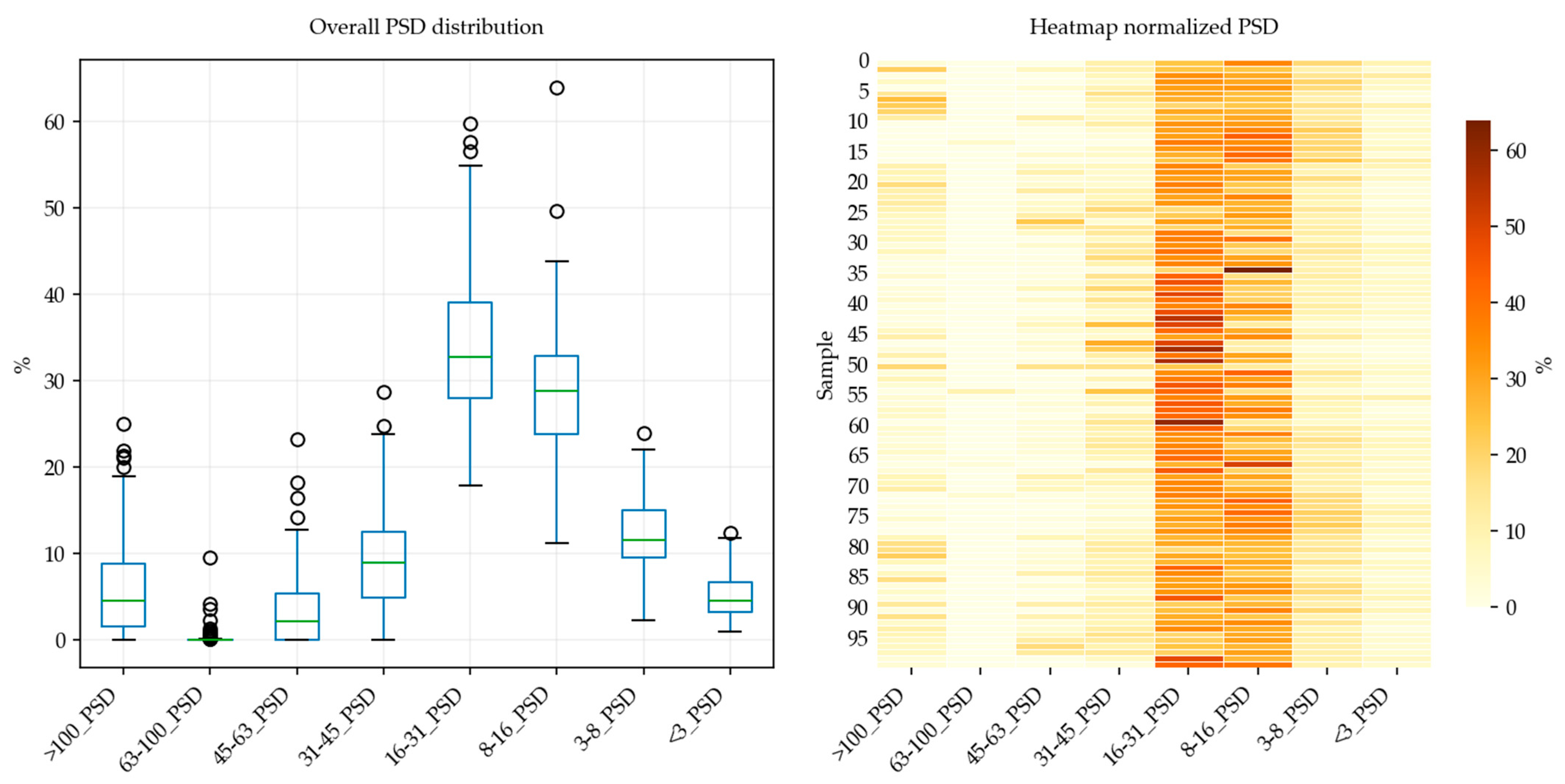
The boxplot analysis (Figure 1) indicates that the PSD across the 100 samples is primarily dominated by intermediate fractions, with the 16–31 mm and 8–16 mm sieves showing the highest median contributions (approximately 32% and 28%, respectively). These fractions therefore constitute the main component of the samples. The 3–8 mm fraction provides a secondary contribution, whereas the 63–100 mm fraction is consistently underrepresented across the dataset. Both the 8–16 mm and 16–31 mm fractions also exhibit the greatest variability, characterized by wide dispersion and the presence of outliers, which suggests significant heterogeneity among samples within the dominant size classes.

The normalized heatmap further corroborates these observations, highlighting the prevalence of the 16–31 mm and 8–16 mm fractions through consistently higher intensity values across most samples. In contrast, the <3 mm and 63–100 mm fractions are characterized by uniformly low intensity, indicating limited contribution to the overall PSD. Notably, a subset of samples (e.g., 1, 5–9, and 20) displays elevated values in the >100 mm fraction, suggesting the presence of distinct sub-populations with increased coarse material content and confirming heterogeneity within the dataset.

Finally, the application of Equation (4) resulted in the classification of 53 samples as coarse and 47 as fine, confirming a slight predominance of coarse material within the investigated population. The classification threshold was set at a coarse/fine ratio of 1.176, corresponding to the median of the ratio distribution after excluding 6 observations (6.0% of the dataset) identified as high-value outliers via the IQR criterion (upper fence = 2.578). To assess the sensitivity of the classification to the threshold choice, alternative thresholds were tested at ±10% and ±20% of the reference value. Variations of ±10% (thresholds of 1.058 and 1.293) resulted in 8 and 9 samples changing class, respectively, whereas ±20% variations (thresholds of 0.941 and 1.411) affected 17 and 20 samples out of 100. These results indicate a moderate sensitivity to threshold selection in the ±10% range, and a higher but still bounded sensitivity at ±20%, supporting the robustness of the median-based approach for this dataset.

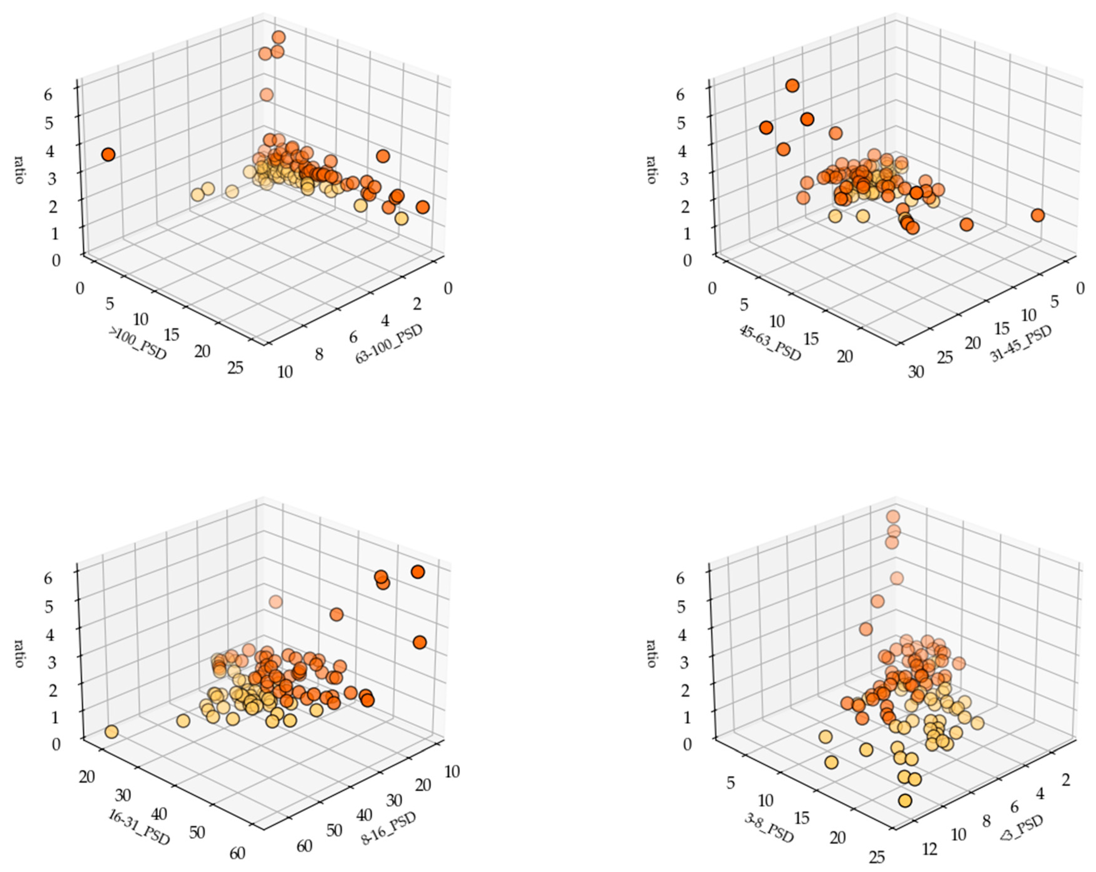
The 3D scatter plots (Figure 2) illustrate the distribution of samples according to R (Equation (3)) across pairwise PSD fractions, highlighting a clear separation between classes. Samples classified as coarse systematically occupy higher positions along the R axis regardless of the specific fraction pair considered, confirming the robustness of the ratio as a discriminant parameter. The spatial arrangement of points also suggests internal variability within each class, particularly among intermediate fractions, consistent with the heterogeneity previously observed in Figure 1.

3.2. Multivariate Structure of PSD Classes

PERMANOVA revealed a statistically significant difference in multivariate space between the two PSD classes (pseudo-F = 22.93, p = 0.001, 999 permutations, n = 100), indicating that the two groups occupy distinct regions. However, the subsequent PERMDISP test also returned a significant result (F = 11.15, p = 0.002, 999 permutations), suggesting that the two groups differ not only in their centroids but also in their within-group dispersion. Thus, the PERMANOVA result may partly be influenced by differences in multivariate variability rather than solely by differences between groups. For this reason, the PERMANOVA outcome should be interpreted with caution, as the assumption of homogeneous dispersions was not met.

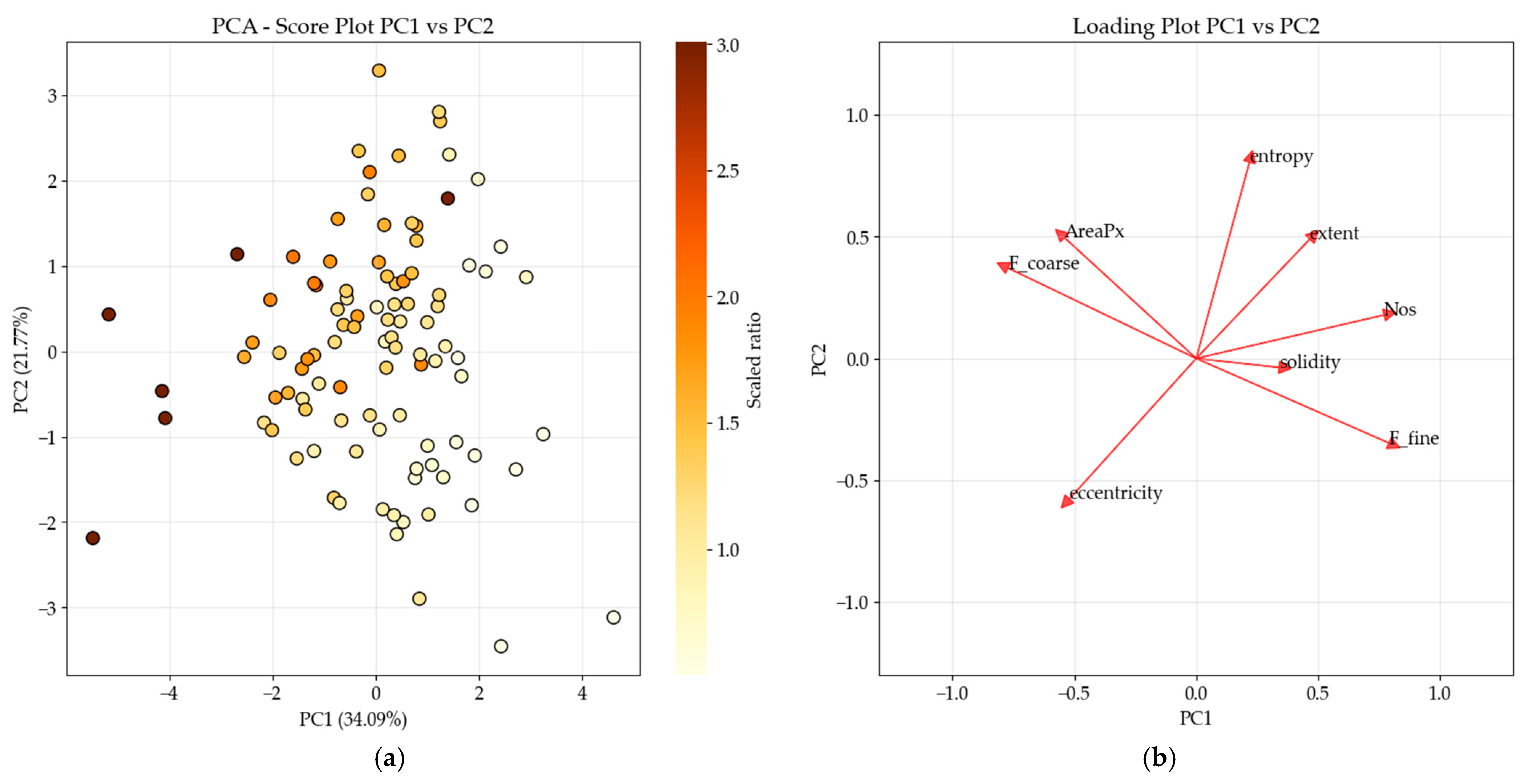
However, the PCA biplot of the first two PCs (Figure 3), which together account for approximately 56% of the total variance, visually supports the separation between the two classes, with a clear separation among them along the PC1 (Figure 3a). Examining the loading plot (Figure 3b), the relationships among variables in multivariate space reveal a strong inverse correlation between $F_{\mathrm{fine}}$, the PSD macro-variable derived from Equation (1), and $Are{a}_{PX}$. Thus, samples characterized by a finer PSD tend to generate smaller shadows, whereas an increase in the coarse fraction corresponds to larger average shadow areas.

The orientation of the vectors associated with $F_{\mathrm{fine}}$, $F_{\mathrm{coarse}}$, and $N_{os}$ suggests a correlation between sample coarseness and the number of generated shadows: coarser samples tend to produce fewer but larger shadows, while finer samples generate a greater number of smaller ones. This relationship, although weaker, is consistent with the findings of previous studies [27,34]. $N_{\mathrm{os}}$ also appears slightly inversely correlated to $Eccentricity$, indicating that a greater number of shadows is associated with more circular and less elongated shapes. While the near-perpendicular orientation between $F_{\mathrm{fine}}$ and $Eccentricity$ indicates an absence of direct relationship between the two variables, the weak covariation between $N_{\mathrm{os}}$ and $F_{\mathrm{fine}}$ still suggests an indirect effect of grain size on shadow morphology: finer samples tend to produce more shadows, which are on average more compact and circular in shape. Overall, PC1 primarily captures the gradient related to PSD and its influence on $Are{a}_{PX}$ and $N_{os}$, whereas PC2 reflects morphological and structural shadow properties, including elongation ($Eccentricity$), spatial coverage ($Extent$), and image complexity ($Entropy$).

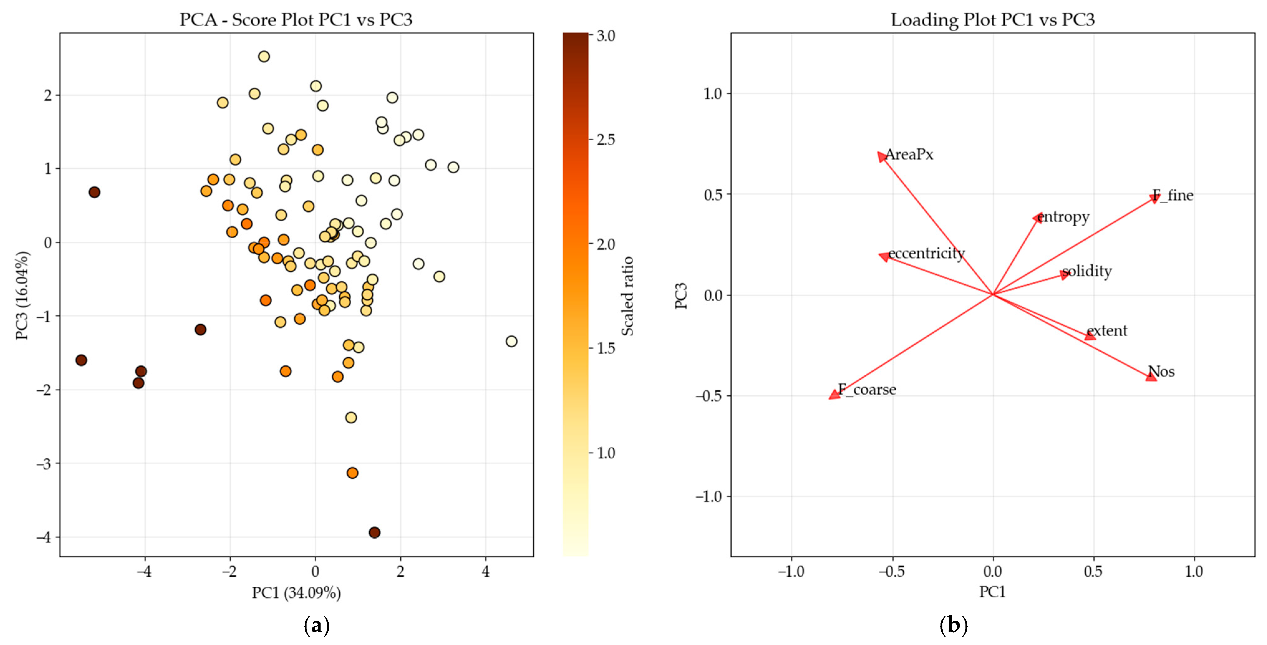
In the PC1-PC3 loading plot (Figure 4b), PC3 accounts for 16% of the total variance, bringing the cumulative explained variance of the first three components to approximately 72%. The most distinctive feature of this axis is the strong positive loading of $Are{a}_{PX}$ combined with the negative loadings of both $F_{\mathrm{coarse}}$ and $N_{\mathrm{os}}$. This configuration suggests that PC3 captures a size-driven source of variability: samples dominated by coarse fractions, which generate fewer shadows, tend to produce larger individual shadow areas, whereas finer samples, despite yielding a higher number of shadows, show a reduction in mean shadow size, likely reflecting geometric fragmentation of shadow coverage as grain number increases. $Eccentricity$ retains a weak negative projection on PC3, consistent with its behaviour in PC2, while $F_{\mathrm{fine}}$, $Entropy$, and $Solidity$ cluster with moderate positive loadings on both PC1 and PC3, confirming their co-variation with fine content.

In conclusion, these results effectively synthesize the multifaceted nature of the dataset, demonstrating that the interplay between PSD variables and shadow metrics serves as a robust and reliable basis for characterizing the analyzed classes/sample discrimination.

3.3. PSD Classification Model Results

This section presents the performance of the SVC models developed for PSD classification. First, model performance is analyzed as a function of the number of included features, comparing the accuracies during training (CV-Train), validation (out-of-fold, OOF) and independent test set (Section 3.3.1). Next, a frequency-based evaluation of feature importance is reported (Section 3.3.2). Finally, overall model behaviour is summarised across all evaluated configurations (Section 3.3.3).

3.3.1. Model Performances Based on Number or Features

Model assessment by number of features reveals a consistent pattern across training, validation, and test phases. Single-feature models show the most limited average performance across all stages (CV-Train = 0.63, OOF = 0.59, Test Accuracy = 0.53, Recall = 0.49, Specificity = 0.58), reflecting the restricted discriminative capacity of each predictor taken individually.

With two features, all metrics improve moderately (CV-Train = 0.68, OOF = 0.65, Test Accuracy = 0.57, Recall = 0.55, Specificity = 0.59). Three-feature models show a more pronounced increase in training score (CV-Train = 0.77) alongside further gains in OOF and test performance (OOF = 0.69, Test Accuracy = 0.58, Recall = 0.62), suggesting that a third feature meaningfully contributes to capturing the variability of the data.

Four-feature models achieve the highest average performance on the independent test set (CV-Train = 0.80, OOF = 0.70, Test Accuracy = 0.62, Recall = 0.66, Specificity = 0.58), representing the optimal point in the trade-off between model complexity and generalization capability. Notably, the gap between OOF and the independent test set remains moderate (approximately 0.10), suggesting that a limited overfitting.

Beyond four features, a divergence between training and test performance becomes apparent. Five-feature models maintain a high CV-Train (0.78) and OOF (0.69), but Test Accuracy drops to 0.59 and Specificity declines to 0.51, indicating that gains observed during cross-validation do not fully transfer to the independent test set. The six-feature model shows the highest OOF (0.70) paired with a CV-Train of 0.80, yet Test Accuracy falls to 0.57, Specificity drops to 0.43, consistent with a progressive tendency towards overfitting and bias toward the positive class as dimensionality increases.

Overall, these results indicate that four features represent the optimal balance between sensitivity and specificity across all evaluation phases, whereas increasing the number of features beyond this threshold produces an increasing train–test discrepancy without stable gains in generalization (

Table 2. Average performances of the best models per number of features.

Features	Train Accuracy	OOF Accuracy	OOF Std. Dev.	Test Accuracy	Test Precision	Test Recall	Test Specificity
1	0.63	0.59	0.09	0.53	0.53	0.49	0.58
2	0.68	0.65	0.08	0.57	0.60	0.55	0.59
3	0.77	0.69	0.09	0.58	0.60	0.62	0.53
4	0.80	0.70	0.08	0.62	0.64	0.66	0.58
5	0.78	0.69	0.08	0.59	0.61	0.66	0.51
6	0.80	0.70	0.10	0.57	0.58	0.69	0.43

1 = Nos; 2 = Nos, Extent; 3 = Nos, Extent, Eccentricity; 4 = Nos, Extent, Eccentricity, Entropy; 5 = Nos, AreaPx, Solidity, Extent, Eccentricity; 6 = Nos, AreaPx, Solidity, Extent, Eccentricity, Entropy.

).

3.3.2. Feature Contributions

Among the evaluated feature subset combinations, the 20 best-performing models were identified separately by OOF accuracy and by test accuracy, yielding two parallel frequency-based relevance analyses. For each ranking, the frequency of occurrence of each feature across the top-20 models was computed, together with a normalized weighted score proportional to the cumulative accuracy of the models in which the feature appeared. Collectively, both sets of top-20 models included all six candidate features at least once.

$Extent$ emerged as the most recurrent feature in the OOF-based ranking (frequency = 16, weighted score = 0.2334) but showed markedly lower occurrence on the test set (frequency = 7, weighted score = 0.11), suggesting that its contribution may be more context-dependent and less stable across evaluation conditions.

${Area}_{PX}$ displayed consistent presence across both rankings (OOF: frequency = 15, weighted score = 0.22; test: frequency = 14, weighted score = 0.21), pointing to a reliable and moderate relevance regardless of the evaluation set.

$N_{os}$ showed an inverse pattern between the two rankings: it appeared with intermediate frequency among the top OOF models (frequency = 13, weighted score = 0.19) but was the most recurrent feature on the test set (frequency = 15, weighted score = 0.23), suggesting that its discriminative value may be more apparent on unseen data than during OOF validation.

$Entropy$ displayed broadly consistent presence across both rankings (OOF: frequency = 11, weighted score = 0.16; test: frequency = 13, weighted score = 0.20), indicating a stable and moderate contribution to model performance.

$Solidity$ ranked fifth in both analyses (OOF: frequency = 8, weighted score = 0.11; test: frequency = 7, weighted score = 0.10), reflecting a marginal and consistent role.

Finally, $Eccentricity$ ranked last in the OOF-based ranking (frequency = 6, weighted score = 0.08) but showed comparatively higher recurrence on the test set (frequency = 10, weighted score = 0.15), suggesting that its discriminative value may emerge more clearly on unseen data.

It should be noted that these rankings reflect co-occurrence patterns rather than causal feature importance, and should be interpreted as exploratory indicators of feature relevance, complementary to the classification metrics reported above.

3.3.3. Overall Performance

Considering all 63 evaluated configurations, the average cross-validation accuracy was 0.75 ± 0.09, with a peak of 0.93, while the average test accuracy was 0.58 ± 0.08.

However, a closer examination of the top-20 models ranked by test accuracy reveals substantially higher performance. In this subset, test accuracy ranges from 0.63 to 0.76, the best configuration (two features, $N_{os}$ and $Entropy$) having with a recall of 0.94 and a specificity of 0.57. Notably, this model yields only one false negative and six false positives on the test set (TP = 15, FP = 6, FN = 1, TN = 8), indicating a strong ability to detect coarse samples while maintaining a moderate but non-negligible capacity to correctly identify fine ones.

Among the top-20 models, the median test accuracy is 0.66, and eight configurations reach or exceed this value. The highest specificity observed in this group is 0.643 (achieved by three different models, e.g., $N_{os}$, $Are{a}_{PX}$, $Entropy$), whereas the highest recall reaches 0.937 (exclusively by the top model). Across these top performers, recall (0.88 ± 0.06) consistently exceeds specificity (0.63 ± 0.09), reflecting a persistent bias toward the coarse class. This asymmetry is likely due to both the moderate class imbalance in the dataset and the intrinsically higher separability of coarse samples, which generate fewer and larger shadows with more distinct patterns. Nevertheless, these findings remain preliminary. The limited sample size amplifies variability and may overestimate the performance gap between classes. Increasing the number of observations is expected to improve both model stability and the balance between sensitivity and specificity.

4. Conclusions

The present study provides a preliminary yet structured assessment of the applicability of the Shadow Size Distribution (SSD) approach for automated classification of wood chip particle size distribution (PSD) under bulk conditions. Despite the preliminary nature of the study, the statistical analyses consistently demonstrate that SSD-derived features retain meaningful PSD information.

PCA highlighted clear and interpretable relationships between PSD features and shadow descriptors, especially in terms of shadow number and average area. This confirms that the SSD feature space embeds physically consistent information related to particle size, supporting its validity as a proxy for PSD characterization.

From an operational perspective, the proposed SSD system presents several advantages over conventional sieve-based analysis (ISO 17827-1). Traditional sieving requires approximately 15–20 min per sample, excluding preparation and handling time, and involves manual operations, dedicated laboratory equipment, and operator-dependent variability. In contrast, the SSD approach enables image acquisition and processing within a time scale on the order of seconds to a few minutes, depending on implementation, with minimal operator intervention. This results in a significantly higher throughput and opens the possibility for near-real-time or fully in-line monitoring.

In terms of cost and infrastructure, conventional sieving requires mechanical equipment, periodic maintenance, and labor, whereas the SSD system relies on relatively low-cost components such as camera, controlled illumination, embedded computing unit and software (please refer to the appendix for a more detailed description of the instrumentation, or to the paper that introduced the SSD-analysis [34]). Once deployed, SSD can operate continuously with limited marginal cost per measurement, making it potentially more suitable for high-frequency monitoring scenarios.

Regarding industrial feasibility, the SSD approach is inherently compatible with bulk material conditions, which represent a major limitation for most existing image-based PSD methods. The use of controlled illumination within an enclosed acquisition chamber mitigates the effects of variable ambient lighting. However, challenges related to dust accumulation, lens contamination, and long-term stability under continuous operation must be considered. These issues can be addressed through standard industrial solutions such as protective enclosures, air purging systems, and periodic automated cleaning.

Additionally, the simplicity of the hardware setup facilitates integration into conveyor-based systems or sampling points within biomass handling lines. However, it is important to underline that the present study remains at a laboratory-scale validation stage, and further investigations under real industrial operating conditions are required before full-scale deployment can be considered.

From a classification standpoint, the results indicate a slightly lower predictive reliability for the $PS{D}_{fine}$ class compared to $PS{D}_{coarse}$. This is reflected in consistently lower specificity values relative to recall, suggesting a higher tendency to misclassify fine samples as coarse. This behaviour may be attributed both to dataset imbalance and to intrinsic differences in feature representation: coarse samples tend to generate fewer and larger shadows, resulting in more distinct and separable patterns, whereas fine samples produce a higher number of smaller and more heterogeneous shadows, leading to increased feature overlap and reduced class separability.

From a practical standpoint, the SSD method does not aim to fully replace standardized sieving procedures, which remain necessary for certification and compliance. Instead, it should be viewed as a complementary tool for rapid screening, process monitoring, and early detection of deviations in biomass quality. Its ability to provide frequent, automated measurements can improve process control, optimize combustion efficiency, and reduce operational variability.

Future developments should focus on two main directions. First, expanding the dataset, second, further validation under real industrial conditions is required to quantify system performance in the presence of environmental variability and to refine the hardware configuration accordingly. Additional work should also explore alternative machine learning models and regression-based approaches for direct PSD classification.

Overall, the SSD approach represents a promising step toward the digitalization and automation of biomass quality assessment. While still at a developmental stage, its combination of speed, low cost, and compatibility with bulk conditions supports its potential applicability in industrial settings, particularly for continuous monitoring and decision-support systems in bioenergy supply chains.

5. Patent

The method for analyzing the dimensional class of objects by examining the shadows cast by objects arranged in groups or in bulk is the subject of a pending patent. The pending patent No. 102024000017878 dated 31/07/2024 has been submitted to the Italian Patent and Trademark Office—UIBM and is titled “Computer implemented method for the analysis of the dimensional class of objects”.