A Deep Learning-Based Approach for High-Dimensional Industrial Steam Consumption Prediction to Enhance Sustainability Management

Abstract

The continuous increase in industrialized sustainable development and energy demand, particularly in the use of steam, highlights the critical importance of efficient energy forecasting for sustainability. While current deep learning models have proven effective, they often involve numerous hyperparameters that are challenging to control and optimize. To address these issues, this research presents an innovative deep learning model, automatically fine-tuned using an improved RIME optimization algorithm (IRIME), with the aim of enhancing accuracy in energy forecasting. Initially, the bidirectional gated recurrent unit (BiGRU) exhibited promising results in prediction tasks but encountered difficulties in handling the complexity of high-dimensional time-series data related to industrial steam. To overcome this limitation, a bidirectional temporal convolutional network (BiTCN) was introduced to more effectively capture long-term dependencies. Additionally, the integration of a multi-head self-attention (MSA) mechanism enabled the model to more accurately identify and predict key features within the data. The IRIME-BiTCN-BiGRU-MSA model achieved outstanding predictive performance, with an R² of 0.87966, MAE of 0.25114, RMSE of 0.34127, and MAPE of 1.2178, outperforming several advanced forecasting methods. Although the model is computationally complex, its high precision and potential for automation offer a promising tool for high-precision forecasting of industrial steam emissions. This development supports broader objectives of enhancing energy efficiency and sustainability in industrial processes.

1. Introduction

As estimated by International Energy Agency (IEA), fossil fuels, including coal, oil, and natural gas, make up 80% of global energy use. If current trends continue, energy consumption is expected to rise by over 50% by 2030 [1]. The industrial sector alone is responsible for 37% of global energy use and 18.4% of carbon emissions [2]. With the increasing energy demand in the refining and power generation industries, the production and utilization of high-temperature steam have become crucial [3]. Accurate steam forecasting is essential for ensuring stable and efficient steam network operations, especially in large-scale plants with extensive and complex piping systems [4]. Optimizing energy prediction systems not only improves the quality and consistency of steam delivery but also reduces steam losses and operational costs, contributing to the sustainability of industrial operations [5]. Accurate steam prediction in thermal power generation is crucial for ensuring operational efficiency, system stability, and cost-effectiveness [6]. As thermal power plants rely heavily on steam produced from the combustion of fossil fuels, fluctuations in steam production can significantly impact system reliability. Effective steam forecasting not only optimizes plant performance but also supports sustainable energy management, making it a key factor in addressing the complexities of modern energy supply and demand [7]. The sustainability of steam prediction in thermal power generation, particularly in coal- and natural-gas-fired plants, plays a pivotal role in ensuring the longevity and efficiency of these systems in the face of increasing global energy demands [8], as the reserve of energy resources diminishes and the need for energy grows due to advancements in technology and rising living standards [9]. In order to meet the increasing demand for sustainable development, it is necessary to use the consumable resources of the world in the most productive manner and at the minimum level and to keep its negative effects on human health and environment at the lowest level possible [10]. In addition, by improving the precision of steam demand forecasts through physical, statistical, and hybrid methods, energy providers can significantly reduce waste and enhance the operational sustainability of their power plants [11]. Therefore, the sustainability of steam prediction in thermal power generation is critical for maintaining operational efficiency, reducing energy waste, and optimizing resource use in industrial sectors such as coal- and gas-fired power plants [12]. The purpose of this study is to explore deep learning-based approaches and propose a predictive model, IRIME-BiTCN-BiGRU-MSA, specifically designed for forecasting high-dimensional steam consumption in industrial settings to enhance sustainable management practices.

2. Related Work

Deep learning [13], a key area of focus in artificial intelligence research, is increasingly gaining attention for its ability to leverage vast datasets and extract complex features to accurately predict resource efficiency. By doing so, it plays a critical role in minimizing energy waste and fostering sustainable development. In pursuit of enhancing the accuracy of sustainability-driven efficiency forecasting, Dettori proposed deep learning as a method that can predict blast furnace exhaust gas production and consumption, and demonstrated that deep learning is a faster and smarter way to optimize operational efficiency in engineering processes [14].

Bidirectional gated recurrent unit (BiGRU) is a type of feedback neural network that includes connections of neurons to themselves within the topology of a feedforward neural network. It has garnered widespread attention due to its powerful performance in processing time-series data. Lin et al. used an RNN based on price features to predict financial index fluctuations, demonstrating the potential of RNN in forecasting tasks [15]. Building on this, Fang, Xia et al. proposed an enhanced deep RNN-LSTM algorithm and a stacked GRU-RNN method for renewable energy and power load forecasting, successfully solving the long-term dependency modeling problem and succeeding at capturing time series. The time characteristics in the data significantly improved the prediction accuracy and model stability, demonstrating the advantages of RNN-type models in processing complex time-series data [16,17]. Dai et al. developed a hybrid ensemble optimized BiGRU method for short-term photovoltaic generation forecasting, significantly enhancing the model’s performance in handling non-stationary data and highlighting the adaptability and accuracy of BiGRU in forecasting applications [18]. The advantage of BiGRU lies in its ability to simultaneously capture forward and backward information in time-series data, thereby improving the model’s capacity to handle long-term dependencies and complex features. Additionally, BiGRU demonstrates lower computational complexity and faster training speed compared to traditional RNN and LSTM, making it highly effective for large-scale datasets of industrial steam volumes.

Despite the significant progress made by researchers, certain limitations remain. BiGRU may encounter performance bottlenecks when dealing with extremely long time-series data. Furthermore, there is room for improvement in the extraction of complex features. Therefore, Jia, Fakir and others used LSTM and CNN on real datasets of multiple steam boiler dynamic processes and experimentally concluded that the computational cost of convolutional neural networks (CNNs) is lower, and the CNN-LSTM hybrid model also proved that the hybrid model is the best model for predicting the output power of industrial steam turbines, further demonstrating that integrated CNN can effectively enhance the robustness and generalization ability of the industrial steam consumption prediction model [19,20].

Temporal convolutional networks (TCNs) are a class of convolutional neural networks that include convolutional layers and pooling layers, enabling the extraction of multi-dimensional features from time-series data. TCN have demonstrated their versatility and effectiveness across various predictive tasks, particularly in energy forecasting and industrial applications. Peng et al. developed a local enhancing transformer with a temporal convolutional attention mechanism for predicting the remaining useful life of bearings, illustrating the effectiveness of TCN integrated with other advanced techniques in temporal forecasting [21]. Zhang et al. applied bidirectional temporal convolutional net-works (BiTCNs) for predicting electric vehicle battery swapping demand, demonstrating improved accuracy by processing data from both past and future contexts [22]. Shi et al. applied the TCN-BiGRU neural network to predict PM2.5 concentration, further demonstrating the effectiveness of combining TCN and BiGRU models for forecasting tasks [23]. Incorporating TCNs into these models ensures that they can handle the complexity of energy consumption data while maintaining privacy, demonstrating the ability of TCNs to work in synergy with other techniques to enhance prediction performance and better adapt to the task of industrial steam volume prediction.

However, despite the synergy between TCNs and GRUs enabling robust handling of long-range dependencies, efficient parallel processing, and bidirectional data handling to enhance performance, the feature extraction capabilities and attention mechanisms of these models remain limited. Consequently, some researchers have begun exploring more precise feature extraction models to further enhance their ability to capture features and attend to temporal patterns in time-series data.

The Transformer model, based on the self-attention mechanism, effectively highlights key information, ensuring it persists as time steps increase, thereby better learning dependencies between distant information in time series [24]. However, it requires significant computational resources and can be challenging to train on large datasets. Ma et al.’s method, combining ConvLSTM and self-attention networks, captures spatiotemporal dependencies and improves prediction accuracy [25]. Despite its high performance, it may suffer from high complexity and longer training times. Bi, Zhang, and Wang, among others, proposed a method that integrates a multi-head attention mechanism with LSTM, leveraging the strengths of both LSTM and CNNs to achieve high predictive accuracy and applicability [26,27]. Despite achieving remarkable predictive accuracy and reliability, this integration can be complex and resource-intensive, which may hinder efficient forecasting of industrial steam volumes. Therefore, to reduce the complexity of deep learning models while maintaining predictive performance, the use of automated hyperparameter optimization is particularly crucial.

Deep learning models are complex and nonlinear, making manual adjustment of these parameters time-consuming and challenging to achieve optimal results. Hyperparameter optimization can systematically search and evaluate different hyperparameter combinations, thereby achieving optimal performance within limited computational re-sources and time. Gülmez proposed a deep Long Short-Term Memory (LSTM) network combined with the Artificial Rabbits Optimization (ARO) algorithm for stock price prediction, demonstrating that ARO effectively optimizes LSTM hyperparameters, improving prediction accuracy and robustness [28]. Wang et al. developed a ship energy usage prediction method using Genetic Algorithm (GA) and LSTM, showing that GA significantly enhances the model’s adaptability and accuracy [29]. Guo et al. proposed a Particle Swarm Optimization (PSO) and GRU-based model for goaf coal temperature prediction, which excels in capturing subtle temperature variations and outperforms traditional methods [30]. Li et al. introduced a Bayesian Optimized Spatial-Temporal Attention-enhanced LSTM (BO-STA-LSTM) for building energy prediction, significantly improving prediction accuracy through Bayesian optimization [31]. Naheliya et al. investigated a short-term traffic flow prediction model based on the Moth-Flame Optimization Algorithm (MFOA) and Bidirectional LSTM (Bi-LSTM), achieving higher accuracy and efficiency in traffic flow prediction [32]. In summary, these studies underscore the crucial role of optimization algorithms in tuning hyperparameters for deep learning models, demonstrating that various optimization methods can significantly enhance predictive performance and efficiency. Such approaches are particularly well suited for optimizing prediction models in the context of complex data, such as industrial steam volume forecasting. Table 1 below highlights the research related to the above algorithms.

Table 1. Overview of various deep learning-based methods in forecasting applications.

Method	Key Findings	Limitations	Refs
RNN/LSTM/GRU Models	1. RNN, LSTM, and GRU demonstrate exceptional performance in handling complex time series and capturing long- and short-term dependencies.	1. May encounter performance bottlenecks when processing extremely long time-series data.	[15,16,17,18]
	2. BiGRU excels in capturing both forward and backward information in time series, offering advantages in computational efficiency.	2. Limited capability in extracting complex features.
TCN and Hybrid Models	1. TCN is effective in extracting multi-dimensional features from time-series data, making it suitable for a variety of predictive tasks.	1. Limited feature extraction capabilities and attention mechanisms.	[21,22,23]
	2. The combination of TCN with BiGRU enhances the ability to handle long-term dependencies and complex data.	2. Still room for improvement in certain applications.
Transformer and Variants	1. The Transformer, based on self-attention mechanisms, excels in learning long-range dependencies.	1. High computational resource requirements and training complexity.	[24,25,26,27]
	2. Integrating multi-head attention mechanisms and convolutional layers enhances feature capture and prediction accuracy.	2. High complexity, with lengthy tuning and training times.
Hyperparameter Optimization Algorithms	1. Hyperparameter optimization algorithms significantly improve the predictive performance and efficiency of deep learning models.	1. Challenges in achieving optimization within limited computational resources and time.	[28,29,30,31,32]
	2. Systematic search for optimal hyperparameter combinations enhances model adaptability and accuracy.	2. Increased complexity may pose challenges in model debugging.

In summary, this research develops a deep learning model specifically designed to address time-series prediction problems characterized by large magnitude, nonlinearity, and strong coupling in industrial steam volume prediction. Initially, BiGRU was utilized to learn both historical and future information, capturing short-term dependencies effectively. However, BiGRU alone faced challenges in handling long sequences due to issues like gradient explosion or vanishing gradients. To overcome these limitations, BiTCN was introduced. By splitting the dataset and inputting it into BiTCN, long sequences were converted into multiple short sequences, reducing spatial complexity and addressing gradient issues. Despite these improvements, there remained challenges in fully capturing the periodicity and intricate dependencies within the time-series data. To further enhance the model’s performance, the multi-head attention mechanism was incorporated. This mechanism allowed the model to focus on various parts of the input data, improving its ability to capture the periodic patterns and long-term dependencies more effectively. However, achieving optimal performance required fine-tuning several hyperparameters, which posed an additional challenge. To address this issue, IRIME is an improved optimization algorithm that surpasses common optimization algorithms such as GA, PSO, and GWO in terms of convergence speed and efficiency in escaping local optima. Therefore, this research will use IRIME for hyperparameter optimization. IRIME combines a good point set strategy, subtraction-average-based optimization, and an Adaptive Cauchy–Gaussian Mutation Optimization Strategy, significantly enhancing the performance of the RIME optimization algorithm. By optimizing parameters such as the learning rate, the number of BiTCN neurons, the number of BiGRU filters, and regularization parameters, the model’s predictive performance and efficiency have been significantly enhanced, aiming to efficiently carry out industrial steam volume forecasting tasks.

The remainder of this paper is organized as follows. In Section 3, the advantages and disadvantages of the model, as well as its structure, are introduced, and the integration of BiTCN-BiGRU-MSA is discussed. Section 4 describes the establishment and improvement of the RIME optimization algorithm and its purpose. Section 5 presents the experimental results of the proposed IRIME-BiTCN-BiGRU-MSA and compares its performance with SOTA methods. Section 6 summarizes this research.

3. Model Establishment

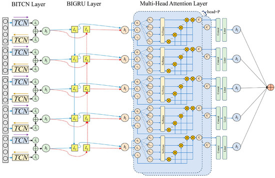
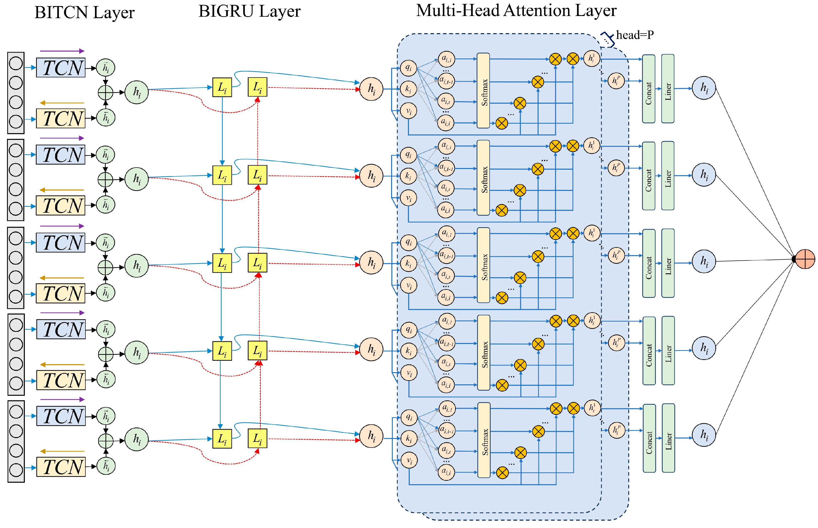
In this research, a sophisticated deep learning model designed to enhance data processing capabilities and improve prediction accuracy is introduced. While TCN layers excel at extracting spatial features, they often fall short in capturing long-term dependencies in time-series data. To overcome this limitation, GRU layers that process information from both past and future states are incorporated, thereby significantly improving time-series prediction accuracy. To further enhance the model, bidirectional structures are employed for both the TCN and GRU. This bidirectional approach enables the model to capture dependencies in both temporal directions, offering a more comprehensive understanding of the data. However, BiTCN and BiGRU alone are not sufficient to fully capture complex data interactions and relationships. Therefore, a Multi-Scale Attention mechanism is integrated. The MSA processes multiple information flows in parallel, effectively capturing intricate and dynamic relationships within the data. The combined framework of BiTCN, BiGRU, and MSA is illustrated in Figure 1, showcasing how these components synergistically work together to enhance the model’s performance.

Figure 1. BiTCN-BiGRU-MSA model framework.

3.1. BiGRU

The GRU model, a simplified version of the LSTM, employs recursion to extract global information from time-series data, using specialized gates—namely, the update and reset gates—to mitigate gradient dispersion and facilitate long-term memory retention with reduced computational overhead and retains its effectiveness while featuring a simpler structure, fewer parameters, and improved convergence [33]. To better capture the contextual information in sequential data, GRU employs a bidirectional strategy to improve model performance.

$$D_T=\sigma (w_d[h_{T-1},x_T]+b_d)$$

(1)

where $x$ represents the input data, $h$ represents the output of GRU unit, $d$ represents the reset gate, and $r$ represents the update gate. The update gate determines the degree to which the current prediction point retains information from previous points, and it controls the current input $x_T$ and the hidden state $h_{T-1}$, output $D_T$ between 0 and 1. $\sigma$ represents the sigmoid activation function, which outputs values between 0 and 1, $Te{a}_T$ is the input matrix at time step $T$. $h_{T-1}$ is the hidden state from the previous time step $T-1$. $w_d$ is the weight matrix of the update gate, and $b_d$ is the bias matrix of the update gate.

The reset gate controls how much historical information should be ignored and determines whether the storage unit should remove unnecessary detection features.

$$R_T=\sigma (w_r[h_{T-1},x_T]+b_r)$$

(2)

where $w_r$ is the weight matrix of the reset gate, and $b_r$ is the bias matrix of the reset gate.

The new state ${\stackrel{⌢}{h}}_T$ based on the update gate is calculated.

$${\stackrel{⌢}{h}}_T=tahn(w_h[D_T{h}_{T-1},x_T]+b_h)$$

(3)

where $w_h$ is the weight matrix of the output of GRU unit, and $b_h$ is the bias matrix of the output of GRU unit.

The state $h$ at the current time step $T$ based on the reset gate is calculated.

$$h_T=(1-D_T)h_{T-1}+D_T{\stackrel{⌢}{h}}_T$$

(4)

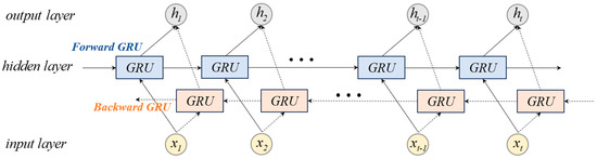
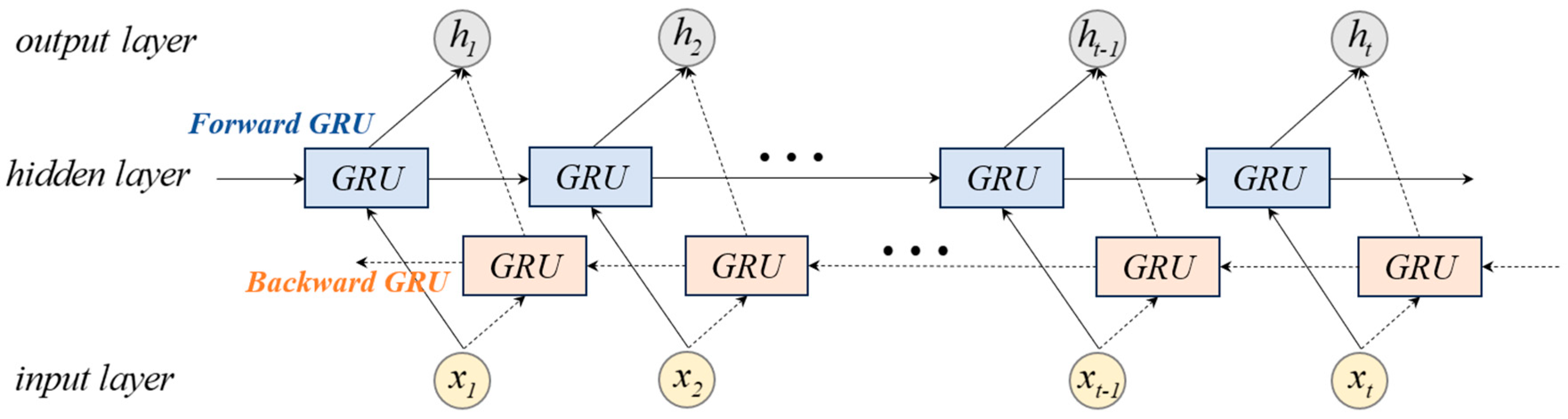
An effective load forecasting model must be capable of extracting hidden features and complex variations from sequential data. However, similar to traditional RNNs, the GRU can only capture forward information. To address this limitation, this research incorporates bidirectional temporal convolution to capture comprehensive information and proposes a BiGRU model. In the encoder, the BiGRU layer is composed of two independent GRU networks. These networks are interconnected at adjacent depths, ensuring that the hidden state from a previous depth can be transferred unidirectionally to the next hidden state. This structure enables feature extraction in both forward and backward directions. Figure 2 illustrates the structural diagram of BiGRU. The BiGRU model can be represented as follows:

$$h_T=F(\overrightarrow{h_T},\overleftarrow{h_T)}$$

(5)

where $\overrightarrow{h_T}$ and $\overleftarrow{h_T}$ represent the hidden states of the forward and backward GRU, respectively. $F$ denotes the method of combining outputs from both directions, such as multiplication, averaging, summation, etc. This research adopts the weighted summation method.

Figure 2. BiGRU structural diagram.

3.2. BiTCN

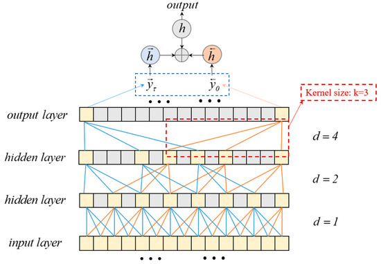
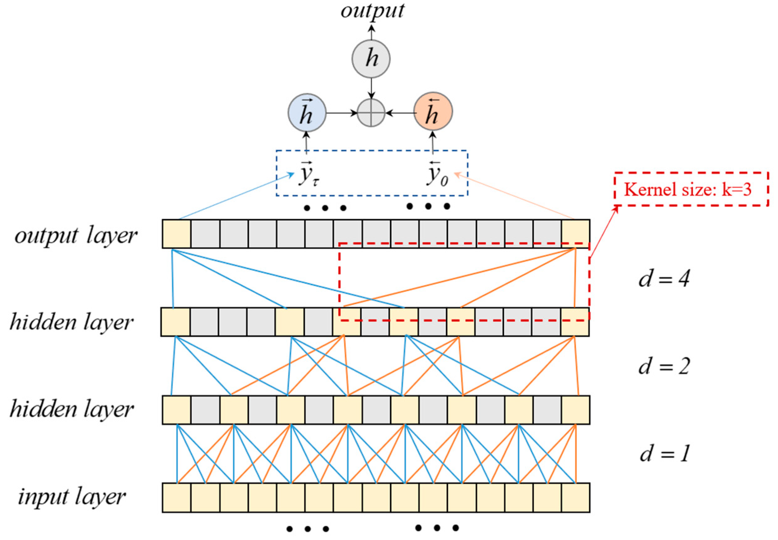
To overcome the limitations of BiGRU in handling high-dimensional sequential data, TCN is introduced. By using convolution operations and causal convolutions, it can capture long-range dependencies with enhanced feature recognition capabilities while maintaining the model’s computational parallelism and stability. TCN is a neural network model designed for time-series prediction, incorporating dilated causal convolution (DCC) and residual connections (RCs) [34]. Traditional TCNs only perform forward convolutions on the input sequence, neglecting the hidden information in the backward direction. This limitation hinders their ability to learn associations between current features and subsequent features. To overcome this issue, this research leverages the capability of BiTCNs to simultaneously capture both forward and backward features of time-series data. This functionality enhances feature extraction, aiding in the more effective identification of long-term dependencies within the data. Additionally, the time-series data are divided into sliding windows, and relevant variables associated with the research objectives are selected to extract features from each window, thereby improving the capture of temporal dependencies. The structure of the BiTCN is illustrated in Figure 3.

Figure 3. BiTCN structural diagram.

To solve the problem of information leakage from the future to the present in traditional convolutional neural networks when dealing with time-series data, this research employs a special convolutional neural network structure, that is, causal convolution. Its principle is to calculate the value $y_r=f(x_1,x_2,...,x_{\tau })$ at time $\tau$ in the previous layer based on the value at time $\tau$ and previous values $[x_1,x_2,...,x_{\tau }]$ in the next layer. The calculation $y_r$ only depends on inputs before the current time point, and $f$ is a one-dimensional causal convolution kernel. To effectively capture the long-term characteristics of sequences, causal convolution requires additional layers or a larger receptive field. Therefore, BiTCN utilizes dilated convolution to achieve a larger receptive field with fewer layers while maintaining the dimensionality of feature mappings. By employing dilated convolution for interval sampling, the complexity of the network structure and the computational burden of the model can be significantly reduced, making the TCN model’s receptive field more flexible and capable of learning a more comprehensive set of time-series information features. For the one-dimensional input sequence $x\in R^n$ and convolution kernel filter $\{0,...,k-1\}\to R$, the expanded convolution of elements in the sequence is defined as follows:

$$h(s)={\displaystyle \sum _{i=0}^{k-1}f(i)}\cdot x_{s-d\cdot i}$$

(6)

where $k$ is the size of the convolution kernel, and $s-d\cdot i$ represents the direction of the past. d is the dilation factor, which determines how many zeros are inserted between two adjacent convolution kernels. After each convolution layer in the input sequence, d grows exponentially, allowing BiTCN to achieve a larger receptive field after several convolutions.

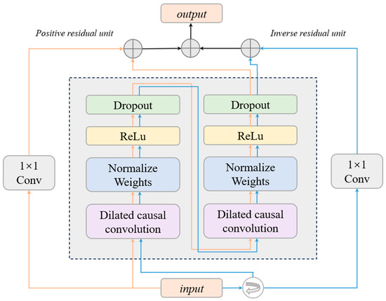
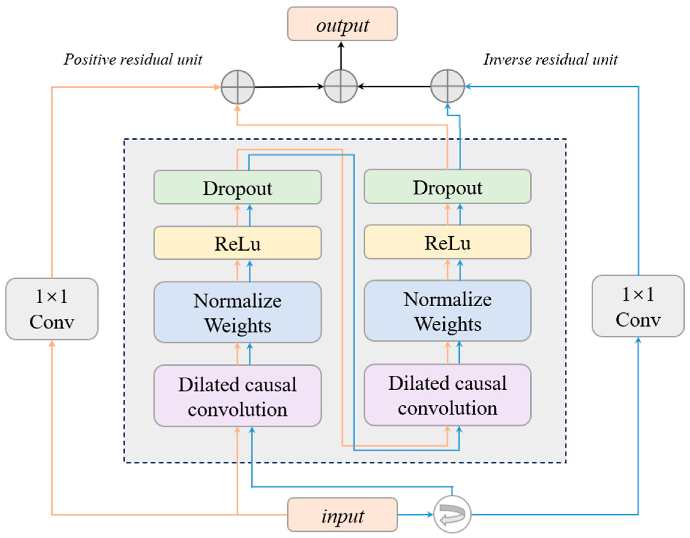
However, the increased receptive field of BiTCN brings issues such as gradient vanishing and slow convergence. Thus, residual blocks are introduced. In each residual module, convolution operations are performed through two layers of dilated convolutions, and weight normalization is applied via Weight Norm to standardize the input to hidden layers and address the gradient vanishing issue. The inclusion of Dropout can effectively solve the problem of model overfitting. The residual connection formula can be represented as follows:

$$o=Activation(x+H(x))$$

(7)

where x is the input data, and $H(x)$ represents the residual network. Through residual connections, gradient vanishing is prevented, making the neural network more stable, while also achieving efficient feature extraction of the sequence. The residual blocks are illustrated in Figure 4.

Figure 4. The structure of residual block in BiTCN.

Therefore, through the superior performance of BiTCN in extracting and utilizing temporal features, it is possible to address the gradient vanishing problem that often impedes BiGRU ability to capture long-term dependencies.

3.3. Multi-Head Attention

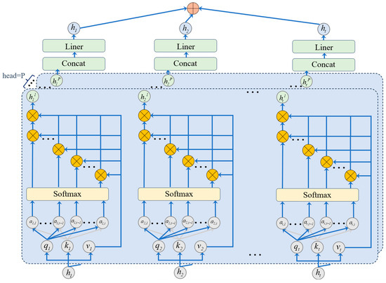
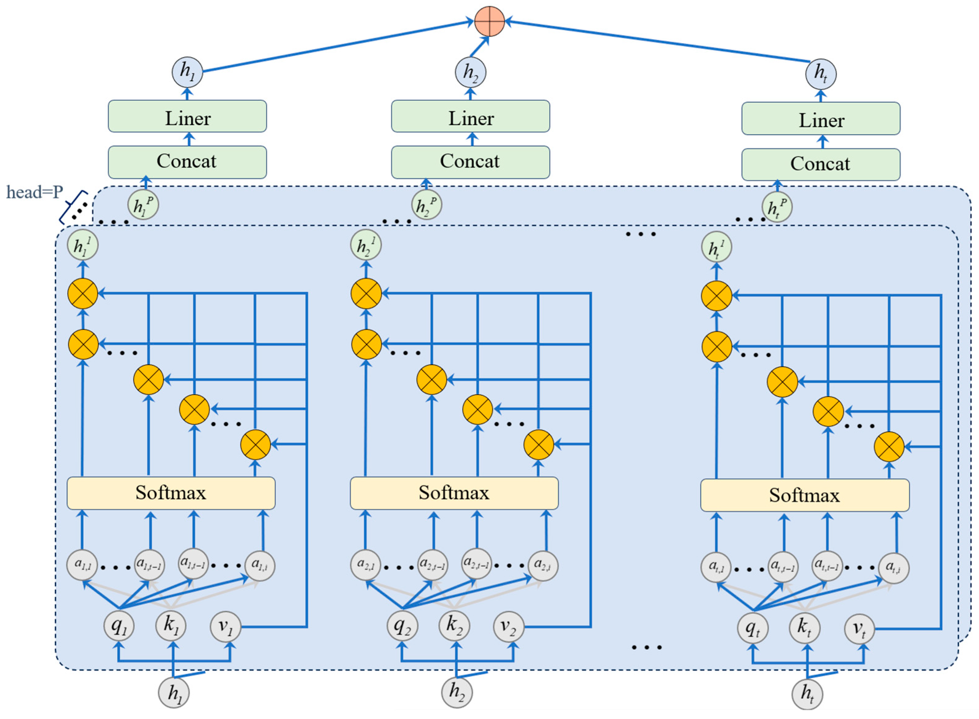
To address the issues of information decay, insufficient memory, and weak local feature extraction encountered by the BiGRU-BiTCN model when processing very long sequences, this research introduces a multi-head self-attention mechanism to enhance the model’s predictive ability. The multi-head self-attention mechanism surpasses the capabilities of the self-attention mechanism [35]. The multi-head attention mechanism allows for the learning of related information across different representational subspaces. Additionally, the introduction of disagreement regularization aims to enhance the diversity of information captured by each attention head, thereby improving the model’s ability to learn the varied and complementary aspects of the data [36]. The structure of the multi-head attention mechanism is illustrated in Figure 5.

Figure 5. Multi-head attention model structure diagram.

The calculation process of the multi-head attention mechanism algorithm is as follows: Suppose the input dimension of the attention mechanism is d and the output dimension is m, the input vector $x_i$ is transformed into key $q_i$, query $k_i$, and value $v_i$ matrices, with the specific calculation formula as follows:

$$q_i=W_q\times x_i$$

(8)

$$k_i=W_k\times x_i$$

(9)

$$v_i=W_v\times x_i$$

(10)

Then, $q_i$, $k_i$ and $v_i$ are divided into vectors according to the number of heads in the attention mechanism, with each head corresponding to the query, key, and value as shown below:

$$q_i=\left[\begin{array}{l}{q}_{i,1}\hfill \\ \cdots \hfill \\ q_{i,c}\hfill \end{array}\right],k_i=\left[\begin{array}{l}{k}_{i,1}\hfill \\ \cdots \hfill \\ k_{i,c}\hfill \end{array}\right],v_i=\left[\begin{array}{l}{v}_{i,1}\hfill \\ \cdots \hfill \\ v_{i,c}\hfill \end{array}\right]$$

(11)

The softmax function is used to normalize the factors, and the calculation formula for the attention weight ${\widehat{a}}_{i,k,j}$ of the j-th attention head of the k-th sequence for the i-th sequence is as follows:

$${\widehat{a}}_{i,k,j}=softmax({\displaystyle \frac{q_{i,j}^T\odot k_{k,j}}{\sqrt{d}}})$$

(12)

Each element in the matrix ${\widehat{a}}_{i,k,j}\in (0,1)$ is composed of k heads together, indicating the distance or similarity from $x_i$ to $x_k$, with a larger value indicating greater similarity. The output $y_i$ of sequence $x_i$ concatenates the attention structure of each head into a column vector by columns, where the calculation formula for the output $y_{i,j}$ of the j-th head is represented as follows:

$$y_{i,j}={\displaystyle \sum _{k=1}^n{\widehat{a}}_{i,k,j}\times v_{k,j},i\in \{1,2,...,n\},j}\in \{1,2,...,s\}$$

(13)

Therefore, after introducing the multi-head attention mechanism, the model can simultaneously focus on different parts of the input sequence. This enables it to capture a wider range of patterns and dependencies within the data, thereby enhancing its overall accuracy and robustness.

4. Improved RIME Optimization Algorithm

To automate the hyperparameter tuning of deep learning models and minimize the excessive consumption of human resources, heuristic algorithms have been widely employed in the automatic optimization of model parameters. These methods are favored due to their robustness and efficiency in navigating the hyperparameter space. RIME [37] is a metaheuristic algorithm inspired by the natural phenomenon of frost and ice formation, similar to other optimization algorithms like Particle Swarm Optimization (PSO) and grey wolf optimizer (GWO) by the natural phenomenon of frost and ice formation. It simulates the growth processes of soft rime and hard rime, developing search strategies for soft rime and penetration mechanisms for hard rime. This approach facilitates both exploratory and exploitative behaviors in optimization methods. However, the traditional RIME tends to converge slowly in the early stages and is prone to getting trapped in local optima in later stages, making it unsuitable for optimizing hyperparameters in deep learning models. To address the limitations of traditional RIME, the research has made several improvements, detailed in the following process:

4.1. Traditional RIME

RIME consists of two main components: specifically, Section 4.1.1 and Section 4.1.2.

4.1.1. Simulating the Movement of Soft Rime Particles Within Frost Ice

This component proposes a soft rime search strategy primarily for exploration within the algorithm. It features a unique method of gradual exploration and development, allowing the algorithm to continually switch between broad exploration and focused development, thereby achieving high efficiency and precision.

4.1.2. Simulating the Intercrossing Behavior Among Hand Rime Molecules

This component introduces a hard rime penetration mechanism primarily for exploiting the algorithm. This mechanism facilitates effective information exchange among molecules through dimensional cross-swapping between ordinary and optimal molecules, enhancing the algorithm’s ability to exploit the search space efficiently.

4.1.3. RIME Model

Assuming a RIME cluster $R$ composed of $n$ rime molecules, and each rime molecule consists of $S_i$ rime particles $d$, cluster $x_{ij}$ can be represented as follows:

$$R=\left[\begin{array}{l}{S}_1\\ S_1\\ ⋮\\ S_n\end{array}\right]=\left[\begin{array}{llll}{x}_{11}& x_{12}& \cdots & x_{1d}\\ x_{21}& x_{22}& \cdots & x_{2d}\\ ⋮& ⋮& \ddots & ⋮\\ x_{n1}& x_{n2}& \cdots & x_{nd}\end{array}\right]$$

(14)

In a light wind environment, the growth height of frost ice is random, allowing frost particles to freely cover most of the substrate surface while slowly growing in the same direction. Inspired by this growth pattern, the soft frost search strategy leverages the strong randomness and coverage of frost particles to rapidly explore the entire search space during early iterations, thereby avoiding local optima. Based on the motion characteristics of frost particles, the formula for updating the frost particle position is as follows:

$$x_{ij}^{new}=x_{best,j}+r_1\beta \cos \theta \left[h\left(U{b}_{ij}-L{b}_{ij}\right)+L{b}_{ij}\right],r_2<E$$

(15)

where $x_{ij}^{new}$ is the updated position of the rime particle, $x_{best.j}$ is the rime particle in dimension $R$ of the best rime molecule within cluster $j$, parameter $r_1$ is a random number within $(-1,1)$, controlling the movement direction of the rime particle, parameter $h$ is the adhesion degree, a random number within $(0,1)$, used to control the distance between the centers of two rime particles, $U{b}_{ij}$ and $L{b}_{ij}$ are the upper and lower bounds of the escape space, respectively, limiting the effective movement area of the rime particle, and parameter $r_2$ is a random number within $(0,1)$, which, along with $E$, controls whether the rime particles coalesce, i.e., whether the position of the rime particle is updated. Tip: i and j in this part are not the same parameters as those in the previous part.

In Equation (16), $\beta$ represents the environmental factor, which simulates the impact of external conditions based on the iteration count to ensure the convergence of the algorithm. It can be represented as follows:

$$\beta =1-{\displaystyle \frac{\left[\frac{Wt}{T}\right]}{W}}$$

(16)

where $W$ is used to control the number of segments in the above step function, with a default value of 5, $t$ is the current iteration number, and $T$ is the maximum number of iterations.

In Equation (17), $\cos \theta$ changes with the number of iterations and can be represented as follows:

$$\theta ={\displaystyle \frac{\pi t}{10T}}$$

(17)

In Equation (18), $E$ is the adhesion coefficient, which affects the condensation probability of a rime molecule and increases with the number of iterations. It can be represented as follows:

$$E={\left({\displaystyle \frac{t}{T}}\right)}^2$$

(18)

Under strong wind conditions, the growth of hard frost is more direct. Inspired by the phenomenon of penetration, the penetration mechanism of hard frost can be applied to update the molecular positions in algorithms. This allows particles within the algorithm to interchange, thereby enhancing the algorithm’s convergence capabilities and ability to escape local optima. Consequently, the formula for particle interchange is as follows:

$$x_{ij}^{new}=x_{best.j},r_3<F^{normr}(S_i)$$

(19)

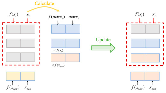
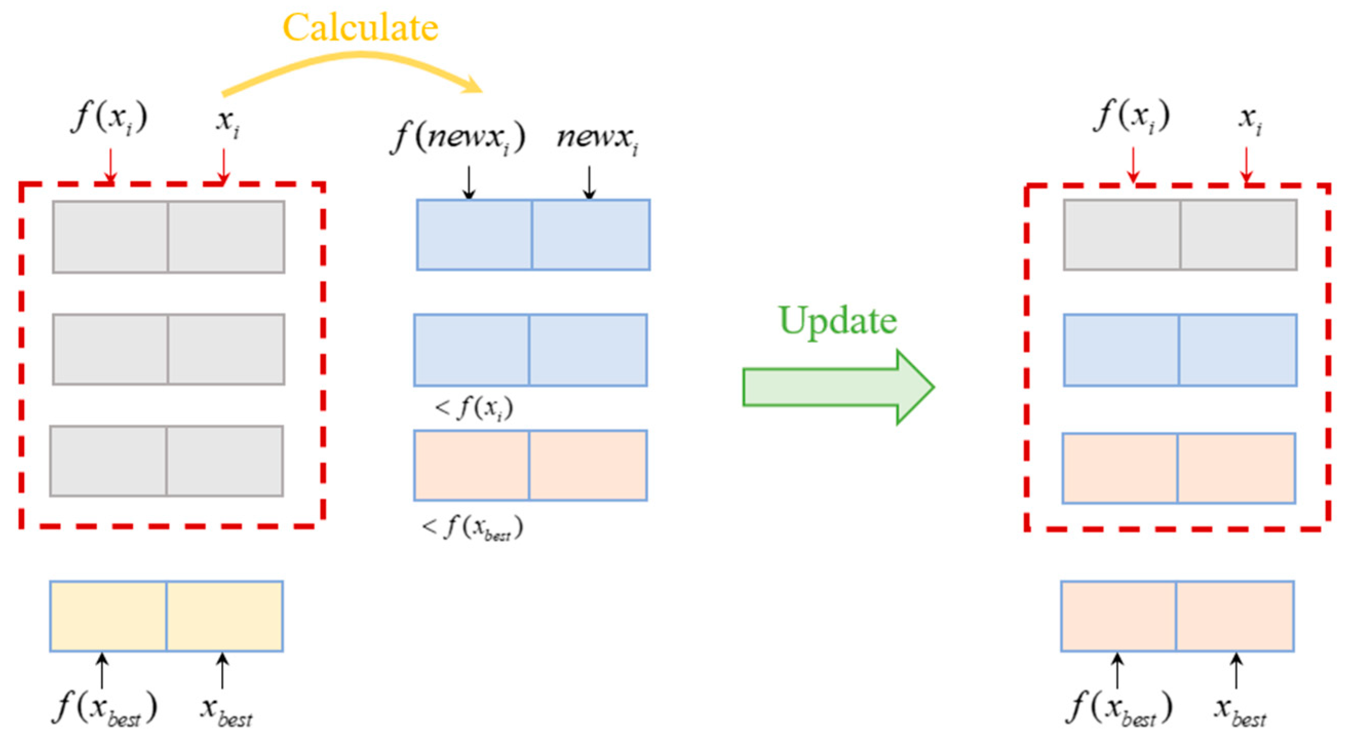
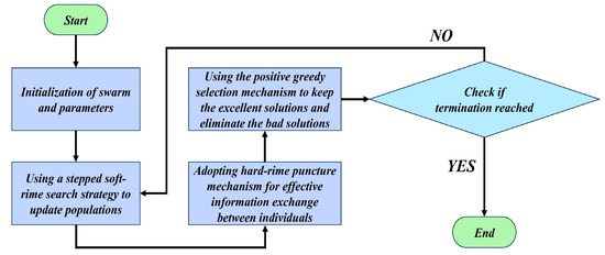
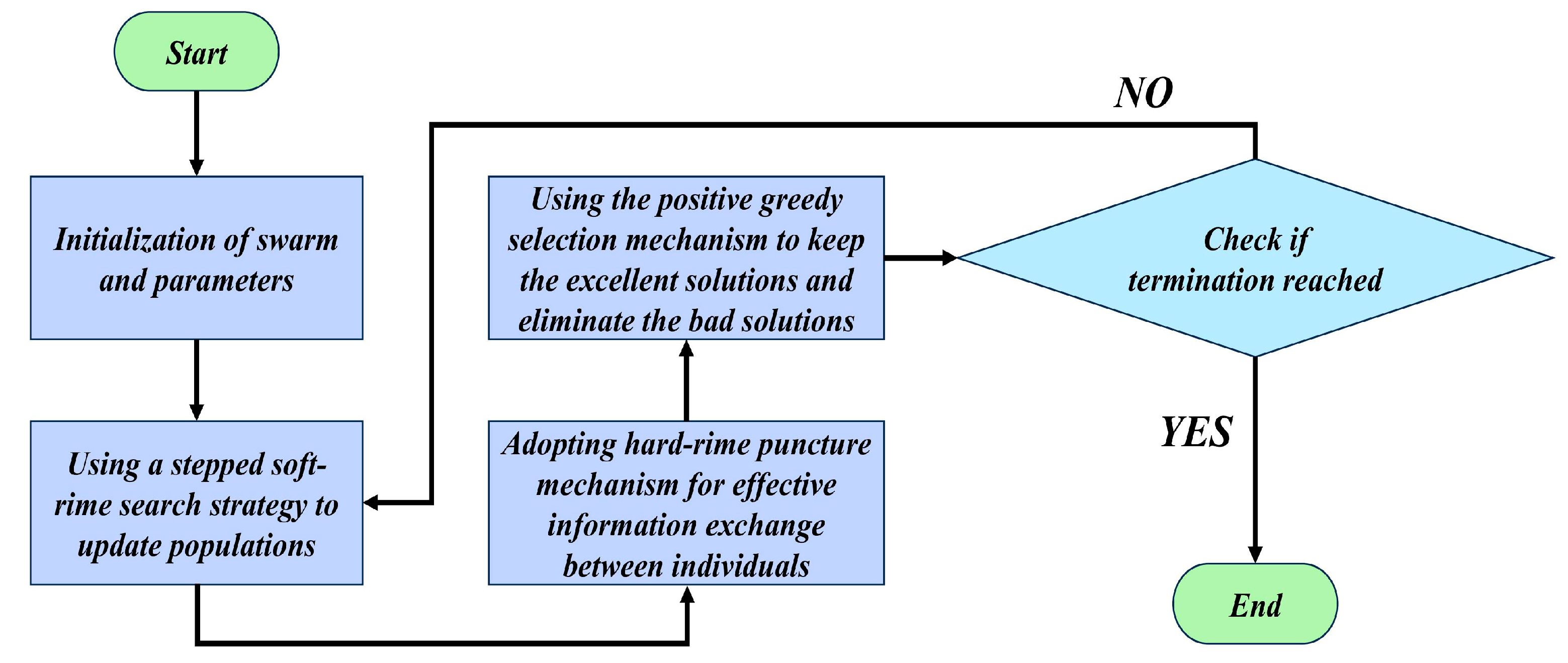
RIME introduces a more proactive greedy selection strategy that not only participates in recording the best solution but also directly influences the update process of the population to enhance global search efficiency. Specifically, this strategy compares the fitness values of agents before and after updates. If the fitness of an agent post-update is better than before, it is replaced with the new solution. This way, agents within the population are continuously replaced with more optimal agents, thereby improving the overall quality of solutions. The specific steps are as follows:

Let $x_i$ represent the position of the $i$ particle, and $f(x_i)$ represent its fitness value. The new fitness value and position are given by $f(new{x}_i)$ and $new{x}_i$, respectively. The global optimum fitness value and corresponding position are represented by $f(x_{best})$ and $x_{best}$. The update mechanism flowchart is shown in Figure 6.

Figure 6. Greedy update mechanism flowchart.

For each particle $i$, first compare its new fitness value with the current fitness value. If the new fitness value is better, update the fitness value and position of the particle to the new values. Next, compare the new fitness value of the particle with the global optimum fitness value. If the new fitness value is still better, further update the global optimum fitness value and its corresponding position.

This method ensures that the overall quality of the population improves after each iteration. Although this may mean that the performance of some agents could be worse than before, overall, it evolves towards a more optimal direction. In this way, the algorithm can more effectively balance exploration and exploitation, driving the solutions towards global optimality. The flowchart of RIME is shown in Figure 7.

Figure 7. Flowchart of RIME.

4.2. Good Point Set Initialization Strategy

The traditional initialization of RIME uses uniformly distributed random numbers, resulting in a uniform and random population distribution. This aids in the extensive exploration of initial solutions within the search space. However, this method does not always ensure the diversity and quality of the population, especially in complex optimization problems. To improve the initial quality of the population and accelerate the algorithm’s convergence speed, a good point set strategy [38] has been introduced to initialize the population.

The principle of the good point set is based on defining a series of special points within a unit cube in D-dimensional Euclidean space, known as “Good Point Set” due to their uniformity and low discrepancy characteristics. For any given r in $G_D$, a good point set can be constructed using a specific sequence generation method. This method relies on a simple formula that generates the coordinates of a point by multiplying the value of r on each dimension by a factor k, and taking its fractional part (denoted as $\{\cdot \}$). Here, k is an integer ranging from 1 to n, where n represents the total number of points generated.

One of the key characteristics of the good point set is its very low discrepancy, meaning the distribution of the good point set is very close to a perfect uniform distribution. The specific magnitude of the discrepancy is given by formula $\phi (n)=C(r,\epsilon )n^{-1+\epsilon }$. Here, $\epsilon$ is an arbitrarily small positive number, and $C(r,\epsilon )$ is a constant that depends only on $r$ and $\epsilon$, indicating that the discrepancy decreases as the number of points n increases.

To generate these special good points, this research opted for a method based on prime numbers p and the cosine function to determine the value of r, with the calculation method as follows:

$$r=2\cos ({\displaystyle \frac{2k\pi }{p}}), k\in [1,\mathrm{D}]$$

(20)

$$p=\min \{x\in P:{\displaystyle \frac{x-3}{2}}\ge D\}$$

(21)

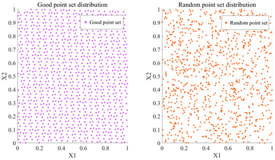
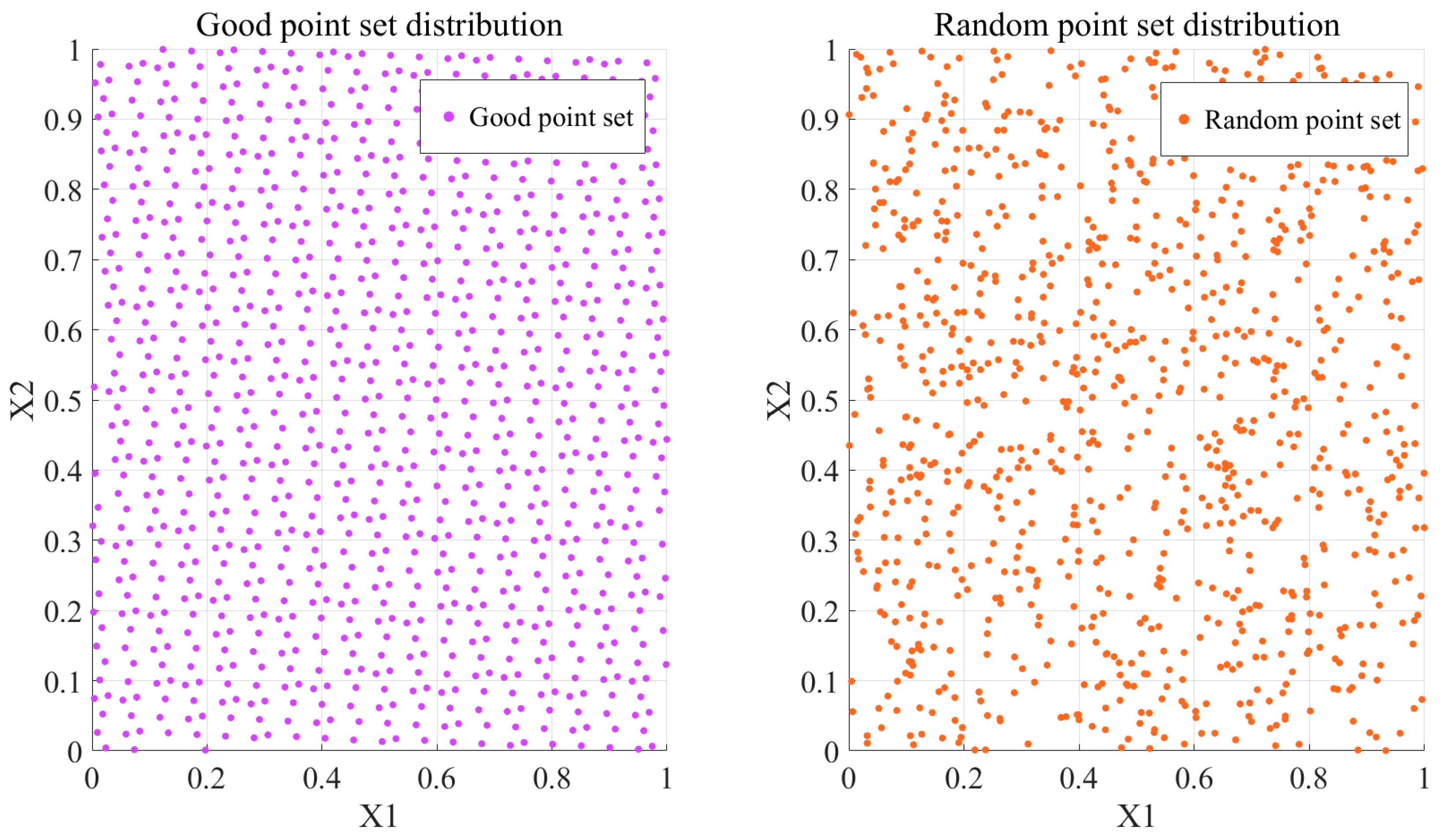
where $p$ is a specific prime number, the smallest prime number that satisfies condition $(p-3)/2\ge D$. This choice ensures that the good points are not only evenly distributed but also possess good mathematical properties, helping to effectively cover the entire search area in multi-dimensional space. The effect is illustrated in Figure 8.

Figure 8. Comparison of good point set strategy and random distribution initialization of population.

By observing the graphic, it is clear that the population of the RIME initialized using the good point set method exhibits a more uniform distribution. This uniform distribution helps improve the convergence speed of the algorithm and reduces the likelihood of the algorithm getting trapped in local optima.

4.3. Search Mechanism Integration Strategy

To address the slower convergence rate of the RIME position update process in the initial iterations, this research introduces the subtractive-average-based optimization (SABO) [39] search strategy to quickly locate potential optimization areas within the search space, thereby accelerating convergence speed and improving the algorithm’s exploration efficiency in the early stages of iteration.

It is noteworthy that the concept of calculating the arithmetic mean in SABO is entirely distinct, based on a special operator “${-}_v$”, which is defined as follows:

$$A{-}_{v}B=sign(F(A)-F(B))(A-\overrightarrow{v}*B)$$

(22)

where $\overrightarrow{v}$ is a vector with dimension m, and the operator “$*$” represents the Hadamard product of two vectors. $F(A)$ and $F(B)$ are the values of the objective functions of the search agents, respectively.

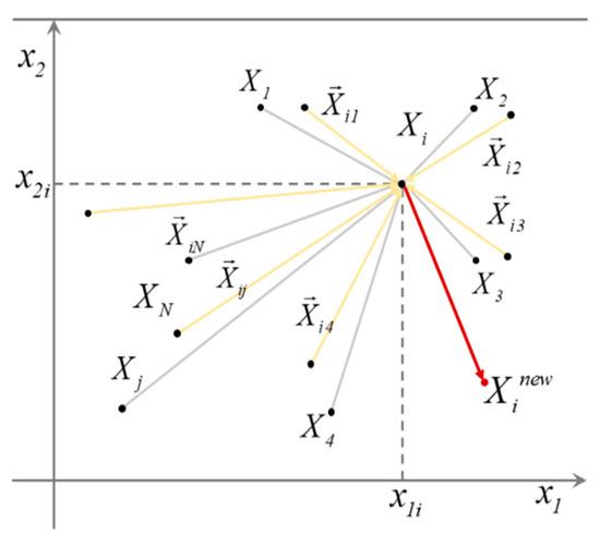
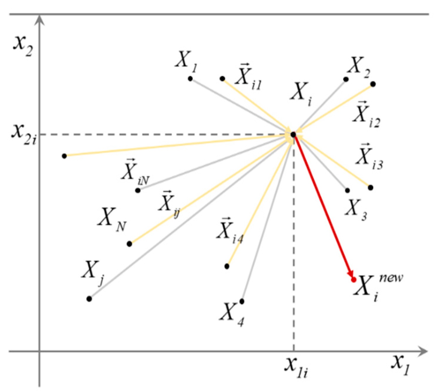
In the SABO search strategy, the new position $x_i^{new}$ is calculated by adding the average difference between the vector ${\overrightarrow{r}}_i$ and all search agents to the current position $x_i$. Here, ${\overrightarrow{r}}_i$ is a vector of dimension $m$, indicating direction and magnitude, and ${\displaystyle \frac{1}{N}}{\displaystyle {\sum }_{j=1}^N(x_i{-}_v{x}_j)}$ calculates the average of the positional differences between agent $i$ and all other agents j, where $N$ is the total number of search agents, that is,

$$x_i^{new}=x_i+{\overrightarrow{r}}_i*{\displaystyle \frac{1}{N}}(x_i{-}_v{x}_j),i=1,2,...,N$$

(23)

This method utilizes global information within the population to guide each search agent towards the direction of the average difference, aiming to find more optimal solution space areas. The schematic diagram of this search strategy is shown in Figure 9.

Figure 9. SABO search implementation process.

Combining the SABO search strategy, the search mechanism can accelerate convergence speed while maintaining exploration diversity, effectively balancing the global and local search capabilities of RIME. Especially in the early stages of iteration, this strategy can rapidly increase the search intensity of the algorithm, accelerate convergence towards the optimization region, and help improve the efficiency and accuracy of the algorithm in solving complex optimization problems.

4.4. Adaptive Cauchy–Gaussian Mutation Strategy

In the later stages of RIME iteration, to enhance exploration capabilities and avoid trapping the algorithm in local optima, an Adaptive Cauchy–Gaussian Mutation Strategy [40] was introduced. This strategy merges the long-tail attribute of the Cauchy distribution with the concentration tendency attribute of the Gaussian distribution. The dynamic adjustment of mutation intensity is achieved by adjusting the weight ratio of the Cauchy and Gaussian distributions during the mutation process, thus adapting to the different characteristics of the search space areas.

Specifically, the strategy implements the update of individual positions through the following expression:

$$x_i=x_i\cdot (\beta \cdot C(0,1)+(1-\beta )\cdot N(0,1))$$

(24)

where $\beta$ controls the weight of the Cauchy and Gaussian distributions in the mutation, dynamically adjusted based on the current iteration number t out of the maximum number of iterations T.

$$\beta =0.9-\log (\mathrm{t}+1)\cdot {\displaystyle \frac{(0.9-0.1)}{\log (T+1)}}$$

(25)

In the initial phase of the iteration process, the algorithm relies more on the Cauchy distribution for detailed local search, which helps to rapidly improve the quality of the solution. As the iterations progress, that is, as the iteration number increases, $\beta$ gradually decreases, thereby gradually increasing the proportion of the Gaussian distribution component, utilizing its concentration tendency characteristics to enhance global search capabilities. This strategy aims to improve the ability to escape local optima and explore unknown areas in the later stages of the algorithm.

When continuous iterations show no significant improvement, indicating a search stagnation, the algorithm increases the proportion of the Cauchy distribution. This mechanism is implemented by monitoring a stagnation counter; if stagnation is detected for five consecutive iterations, the Cauchy–Gaussian mutation is applied. Such an adaptive adjustment mechanism allows the algorithm to intelligently balance exploration and exploitation based on actual progress and historical search effectiveness, effectively avoiding premature convergence while retaining the potential to find global optima.

By introducing the Adaptive Cauchy–Gaussian Mutation Strategy, RIME can more effectively adapt to different stages in the process of solving complex optimization problems, enhancing the algorithm’s robustness and solving efficiency.

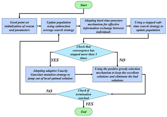
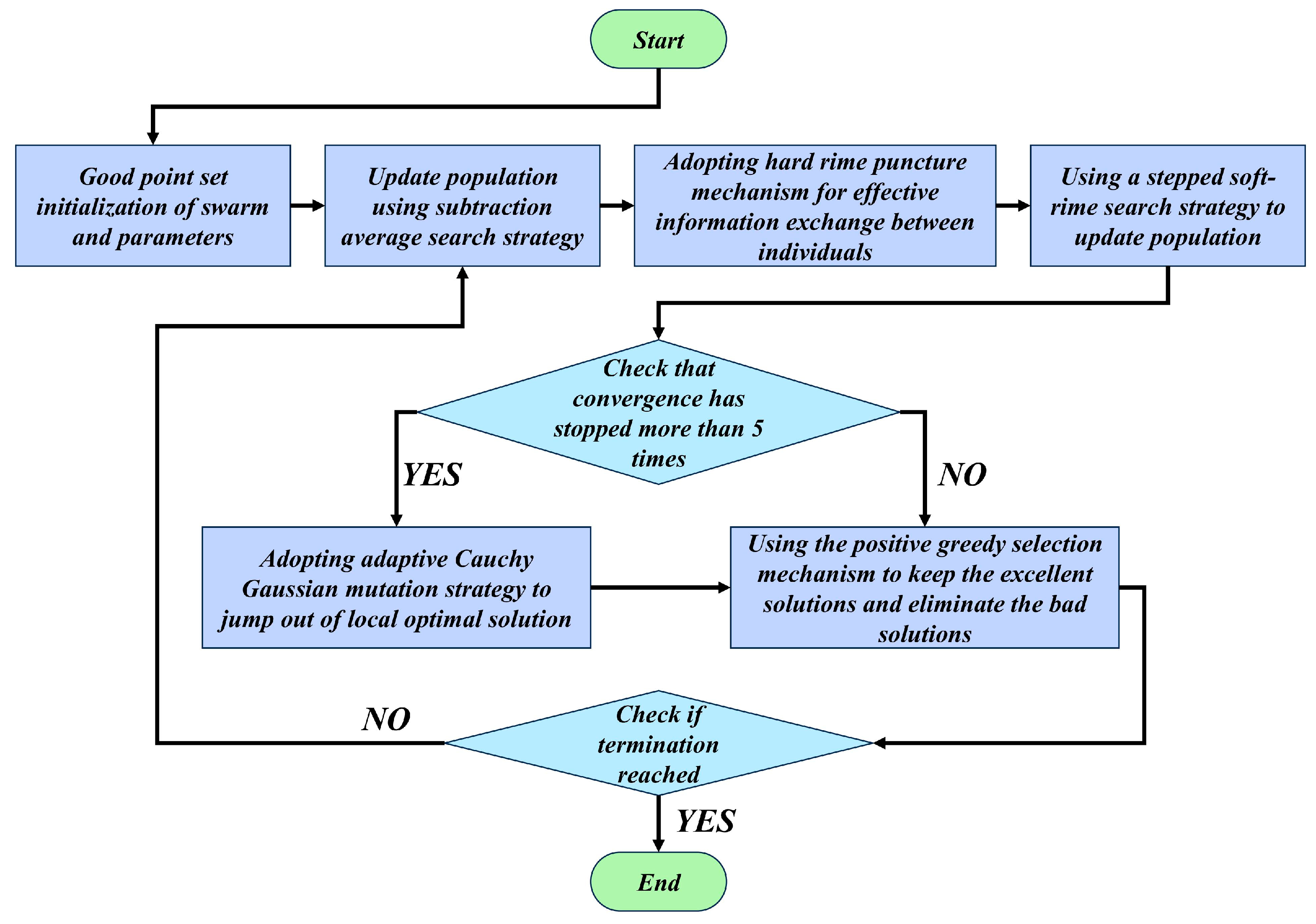
Therefore, the flowchart of the improved RIME is shown in Figure 10.

Figure 10. Flowchart of the IRIME.

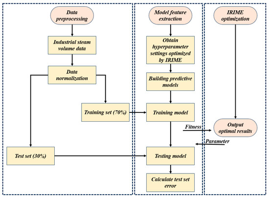
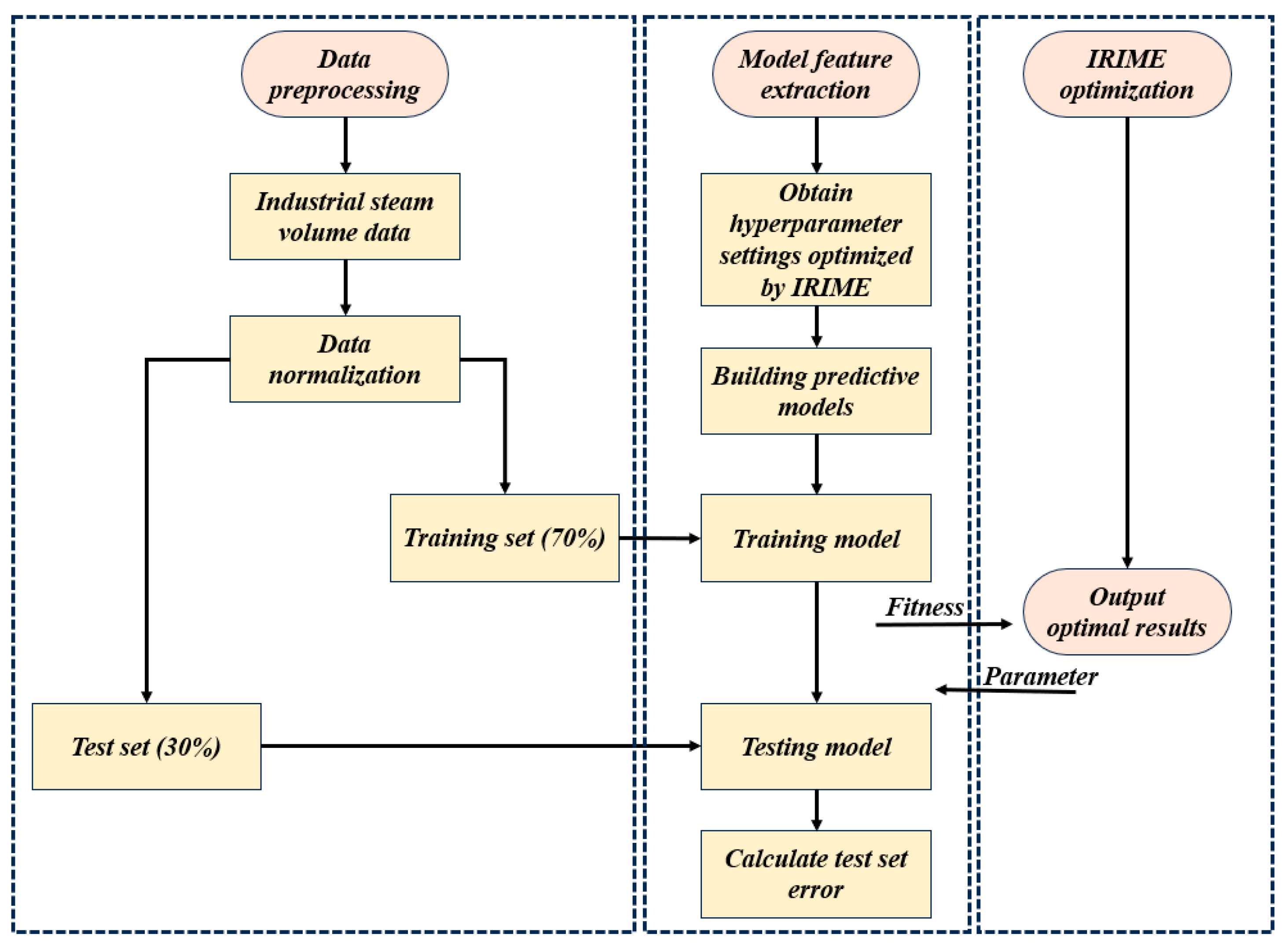
In this research, IRIME is applied to the hyperparameter optimization of a model that integrates BiTCN, BiGRU, and a multi-head attention mechanism. The model’s framework is divided into a data preprocessing module, a model feature extraction module, and an IRIME optimization module. The data preprocessing module performs data preprocessing operations and splits the dataset into training and test sets in a 7:3 ratio. The IRIME optimization module moves the rime particles based on fitness, integrating the good point set strategy, subtractive averaging optimization, and Adaptive Cauchy–Gaussian Optimization Strategy, to achieve iterative optimization of the global optimum solution and the population structure. The feature extraction module decodes the hyperparameters optimized by IRIME, acquiring learning rates, the number of BiTCN neurons, the number of BiGRU filters, and regularization parameters. It then uses the training set for model training, predicts the test set, calculates errors, and feeds them back into the optimization module until the loss function converges. The overall model framework is specifically shown in Figure 11.

Figure 11. IRIME-BiTCN-BiGRU-MSA framework diagram.

5. Experiment and Analysis

5.1. Data Collection

In this experiment, the study utilizes an industrial steam quantity prediction dataset, which is 835 KB in size and comprises 2888 data points with 38 feature variables, labeled as V0–V37 with the target variable is designated as “Target”. This dataset contains desensitized data collected from boiler sensors at a minute-level frequency, aiming to predict steam production based on the boiler’s operating conditions. Table 2 provides descriptive statistics, including the mean, maximum, minimum, and standard deviation values for each field in the dataset. (The industrial steam volume data are sourced from https://tianchi.aliyun.com/competition/entrance/231693, accessed on 16 September 2024).

Table 2. Descriptive statistics.

Fields	Mean	Max	Min	Std
TIME	1444.5	2888	1	833.84
V0	0.1231	2.121	−4.335	0.928
V1	0.0561	1.918	−5.122	0.9415
V2	0.2897	2.828	−3.42	0.9112
V3	−0.0678	2.457	−3.956	0.9703
V4	0.0129	2.689	−4.742	0.8884
V5	−0.5586	0.489	−2.182	0.518
V6	0.1829	1.895	−4.576	0.9181
V7	0.1162	1.918	−5.048	0.9551
V8	0.1779	2.245	−4.692	0.8954
V9	−0.1695	1.335	−12.891	0.9538
V10	0.0343	4.83	−2.584	0.9683
V11	−0.3645	1.455	−3.16	0.8585
V12	0.0232	2.657	−5.165	0.8941
V13	0.1957	2.475	−3.675	0.9228
V14	0.0161	2.558	−2.455	1.0156
V15	0.0961	4.314	−2.903	1.033
V16	0.1135	2.861	−5.981	0.9831
V17	−0.0435	2.023	−2.224	0.6559
V18	0.055	4.441	−3.582	0.9535
V19	−0.1149	3.431	−3.704	1.1089
V20	−0.1862	3.525	−3.402	0.7885
V21	−0.0566	2.259	−2.643	0.7815
V22	0.3029	2.018	−1.375	0.6392
V23	0.156	1.906	−5.542	0.9788
V24	−0.0218	2.423	−1.344	1.0334
V25	−0.0517	7.284	−3.808	0.916
V26	0.0721	2.98	−5.131	0.8898
V27	0.2724	0.925	−1.164	0.2704
V28	0.1377	4.671	−2.435	0.9299
V29	0.0976	4.58	−2.912	1.0612
V30	0.0555	2.689	−4.507	0.9019
V31	0.1278	2.013	−5.859	0.873
V32	0.0208	2.395	−4.053	0.9026
V33	0.0078	5.465	−4.627	1.007
V34	0.0067	5.11	−4.789	1.0033
V35	0.1978	2.324	−5.695	0.9857
V36	0.0307	5.238	−2.608	0.9708
V37	−0.1303	3	−3.63	1.0172
Target	0.1264	2.538	−3.044	0.984

5.2. Experimental Setup

The hardware configuration for the simulation experiment is detailed in Table 3.

Table 3. Configuration description.

Configuration	Description
CPU Model	Intel i7-11800H
Operating System	Windows 10 Pro
System Memory	16.0 GB
GPU Model	NVIDIA RTX-3060
GPU Memory	13.9 GB
Code Environment	MATLAB 2023b

To ensure the reproducibility of the experiment, it is necessary to ensure that the initial parameters of the algorithm are set consistently. The selection of parameters is based on understanding of the problem domain and previous research experience to ensure the effectiveness and generalization capability of the algorithm across different datasets and scenarios. The initial parameter settings for several key algorithms are shown in Table 4.

Table 4. Initial parameter settings.

Algorithm Name	Parameter	Initial Setting
BiGRU BiTCN-BiGRU BiTCN-BiGRU-MSA RIME-BiTCN-BiGRU-MSA IRIME-BiTCN-BiGRU-MSA	Learning Rate	0.0001
	Number of Neurons	10
	Number of Filters	20
	Regularization Parameter	0.00001
	Gradient Threshold	1
	Optimizer	Adam
	Max Training Iterations	100
	Attention Heads	5
	Attention Keys	10
RIME IRIME	Learning Rate	0.0001
	Number of Neurons	10

This study focuses on leveraging deep learning methods to predict industrial steam demand, emphasizing sustainability and efficiency in energy management and process optimization. By learning from historical production data, the project aims to forecast future steam demand without performing preprocessing on this high-dimensional, unstructured dataset, preserving its original complexity. To ensure the model’s effectiveness, a 7:3 data split ratio was implemented, providing sufficient training data while maintaining enough test data to validate the model’s generalization capability. The data are split based on its collection and recording sequence, which captures real-world trends and patterns in steam demand. This approach not only preserves the continuity of the time-series data but also simulates the real-world distribution, enabling a robust evaluation of the model’s predictive performance. To better simulate real-world industrial applications, this study deliberately forgoes data preprocessing to more effectively test the model’s sensitivity to raw data distributions and its ability to identify inherent patterns. This approach aims to demonstrate the potential of deep learning techniques in accurately predicting steam demand, thereby contributing to more sustainable and efficient energy management, optimizing production processes, and reducing energy costs for enterprises.

In this study, the performance of the models is quantified using four metrics: coefficient of determination (R²), mean absolute error (MAE), root mean square error (RMSE), and mean absolute percentage error (MAPE). The significance of these metrics and their specific calculation formulas are outlined as follows:

Coefficient of Determination (R²): This reflects the degree of correlation between the predicted values and the actual values. The closer its value is to 1, the higher is the accuracy of the predictions. The calculation formula is as follows:

$$R^2=1-{\displaystyle \frac{{\displaystyle {\sum }_{i=1}^n{(y_i-{\stackrel{⌢}{y}}_i)}^2}}{{\displaystyle {\sum }_{i=1}^n{(y_i-{\overline{y}}_i)}^2}}}$$

(26)

where $y_i$ represents the actual value, ${\stackrel{⌢}{y}}_i$ represents the predicted value, and ${\overline{y}}_i$ represents the average value of the actual values.

Mean Absolute Error (MAE): This measures the average level of the absolute differences between predicted values and actual values, where a smaller value indicates higher prediction accuracy. The calculation formula is as follows:

$$MAE={\displaystyle \frac{1}{n}}{\displaystyle \sum _{i=1}^n|y_i-{\widehat{y}}_i|}$$

(27)

Root Mean Square Error (RMSE): This measures the square root of the average of the squares of the differences between predicted values and actual values, giving greater weight to larger errors. The calculation formula is as follows:

$$RMSE=\sqrt{{\displaystyle \frac{1}{n}}{\displaystyle \sum _{i=1}^n{(y_i-{\widehat{y}}_i)}^2}}$$

(28)

Mean Absolute Percentage Error (MAPE): This represents the percentage of the prediction error relative to the actual value, used to measure the accuracy of the prediction. The calculation formula is as follows:

$$MAPE={\displaystyle \frac{100\%}{n}}{\displaystyle \sum _{i=1}^n\left|\frac{y_i-{\widehat{y}}_i}{y_i}\right|}$$

(29)

Relative Error (RE): This refers to the difference between the predicted value and the actual value relative to the actual value itself, typically used to evaluate the accuracy of individual predictions. The calculation formula is as follows:

$$RE={\displaystyle \frac{|y_i-{\widehat{y}}_i|}{y_i}}\times 100\%$$

(30)

These evaluation metrics collectively form a comprehensive assessment framework, which not only evaluates the overall predictive performance of the model but also identifies the model’s performance in specific situations. In applications like industrial steam quantity prediction, synthesizing the evaluation results of these metrics can provide a more accurate understanding of the model’s strengths and potential areas for improvement. This enables continuous optimization of the model to achieve higher prediction accuracy.

5.3. Performance Testing

In this study, 12 international standard test functions are employed to evaluate the performance of the improved IRIME. These test functions include single-modal functions, multi-modal functions, and composite benchmark functions, which are used to assess the algorithm’s local search capability, global search expansion capability, and exploration and exploitation capability, respectively. By comparing with existing algorithms such as Grey Wolf Optimization (GWO) [41], Particle Swarm Optimization (PSO) [42], Dragonfly Algorithm (DA) [43], and traditional RIME, a comprehensive understanding of the IRIME performance relative to industry standards can be obtained. This allows for the discovery of its unique characteristics in solving optimization problems. The specific standard test functions are detailed in Table 5.

Table 5. 12 International standard test functions.

Function	Dim	Search Interval
$f_1(x)={\displaystyle {\sum }_{t=1}^n{x}_t^2}$	30	[−100, 100]
$f_2(x)={\displaystyle {\sum }_{t=1}^n\left|x_i\right|}+{\displaystyle {\prod }_{i=1}^n\left|x_i\right|}$	30	[−10, 10]
$f_3(x)={\displaystyle {\sum }_{t=1}^n{({\displaystyle {\sum }_{j=1}^i{x}_j})}^2}$	30	[−100, 100]
$f_4(x)=\max ,\left\{\right|x,|,1\le i\le n\}$	30	[−100, 100]
$f_5(x)={\displaystyle {\sum }_{i=1}^{n-1}[100(x_{i+1}-x_i^2}{)}^2+{(x_i-1)}^2]$	30	[−30, 30]
$f_6(x)={\displaystyle {\sum }_{i=1}^n[x_i^2}-10\cos (2\pi x_i)+10]$	30	[−5.12, 5.12]
$f_7(x)=-20\exp \left(-0.2\sqrt{{\displaystyle \frac{1}{n}}{\displaystyle \sum _{i=1}^n{x}_i^2}}\right)-\exp \left({\displaystyle \frac{1}{n}}{\displaystyle \sum _{i=1}^n\cos (2\pi x_i)}\right)+20+e$	30	[−32, 32]
$f_8(x)={\displaystyle \frac{1}{4000}}{\displaystyle {\sum }_{i=1}^n{x}_i^2}-{\displaystyle {\prod }_{i=1}^n\cos (\frac{x_i}{\sqrt{i}})+1}$	30	[−600, 600]
$\begin{array}{c}{f}_9(x)={\displaystyle \frac{\pi }{n}}\left\{{\displaystyle \sum _{i=1}^{n-1}\begin{array}{l}{(y_i-1)}^2\\ [1+10{\sin }^2(\pi y_{i+1})]\\ +{(y_n-1)}^2\end{array}}\right\}+{\displaystyle \sum _{i=1}^{n}u(x_i,10,100,4)}\\ y_i=1+{\displaystyle \frac{x_i+1}{4}}\end{array}$	30	[−50, 50]
$f_{10}(x)={\left({\displaystyle \frac{1}{500}}+{\displaystyle {\sum }_{j\ne 1}^{25}\frac{1}{j+{\displaystyle {\sum }_{i=1}^2{(x_i-a_{ij})}^6}}}\right)}^{-1}$	2	[−65, 65]
$f_{11}(x)=4x_1^2-2.1x_1^4+{\displaystyle \frac{1}{3}}{x}_1^6+x_1{x}_2-4x_2^2+4x_2^4$	2	[−5, 5]
$f_{12}(x)=-{\displaystyle {\sum }_{i=1}^4{c}_i\exp \left(-{\displaystyle {\sum }_{j=1}^3{a}_{ij}{(x_j-p_j)}^2}\right)}$	3	[1, 3]

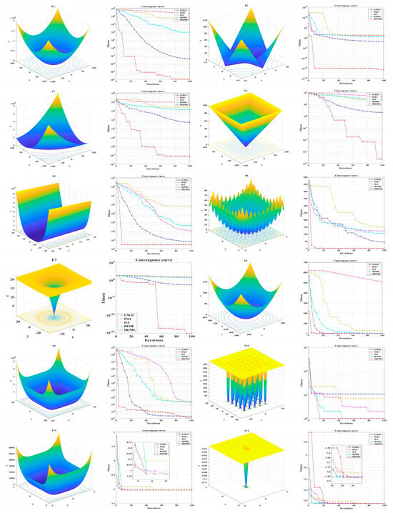
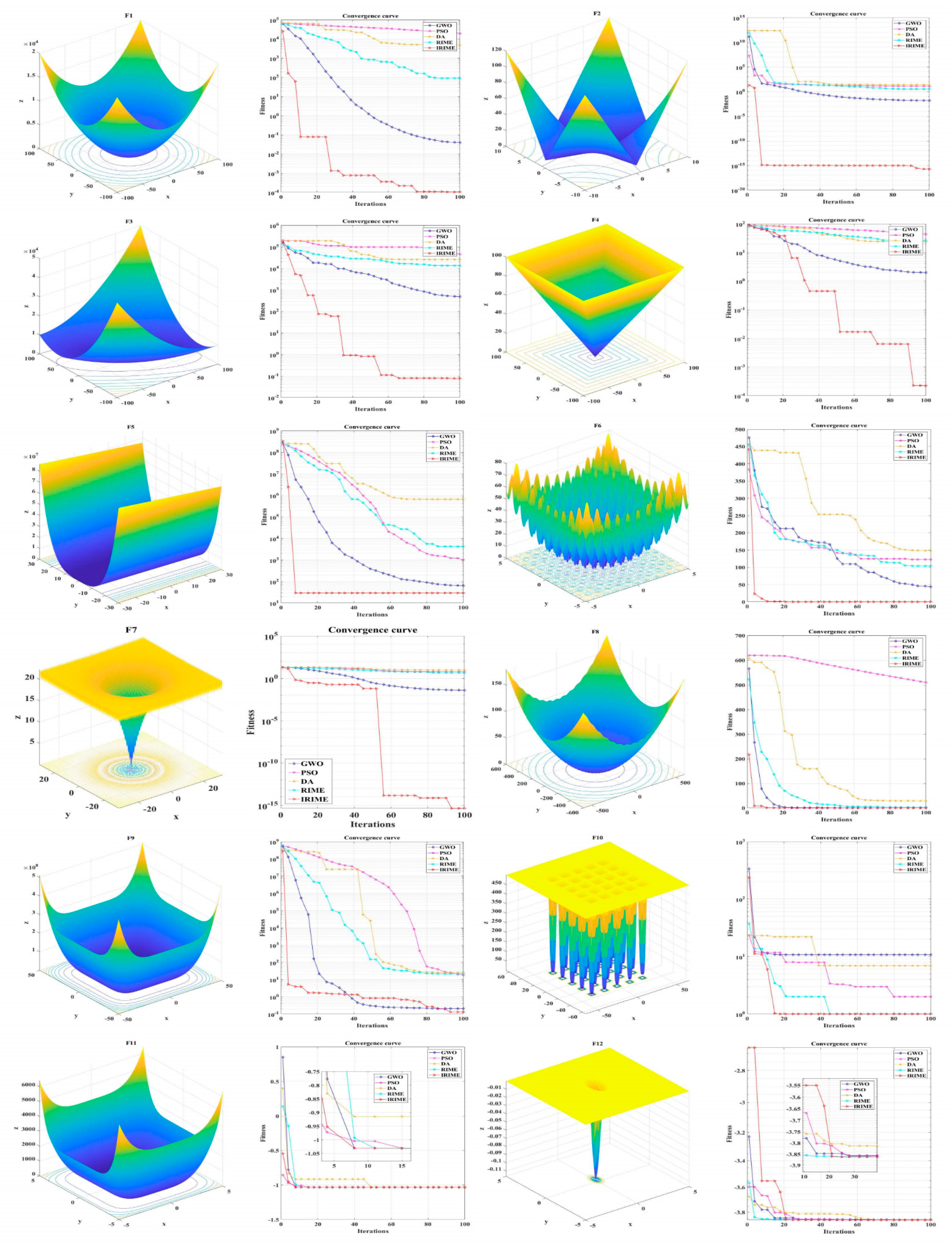
The convergence curves of the IRIME algorithm and other comparable algorithms (including GWO, PSO, DA, and RIME) for various functions are shown in Figure 12.

Figure 12. Convergence curves of IRIME and high-performance algorithms (In this figure, dark blue is GWO, pink is PSO, brown is DA, light blue is RIME, and red is IRIME).

In the experimental setup, the population size was fixed at 30, and the maximum number of iterations was set to 100.

Each test function was independently run 50 times, and the best value was recorded after each run. As shown in Table 6, IRIME consistently demonstrates outstanding global optimal solutions across all 12 test functions. For single-modal functions (F1–F5), IRIME nearly approaches the theoretical optimal value. Taking function F1 as an example, the IRIME algorithm achieves an average of 2.28 × 10⁻⁵, with a standard deviation of only 1.5564 × 10⁴, significantly outperforming other algorithms in these metrics. This result convincingly demonstrates the significant advantages of IRIME in terms of accuracy and stability. Moving on to the multi-modal functions’ (F6–F9) testing phase, the performance of the IRIME is equally impressive. On functions F6, F7, F8, and F9, not only does IRIME achieve excellent scores in terms of averages, but its standard deviation is also the lowest. This indicates that the IRIME exhibits high stability and precision in solving multi-modal problems. For the composite benchmark functions (F10–F12), the IRIME algorithm does not always maintain the lowest average in some cases. However, overall, its performance still demonstrates high computational accuracy and stability. For example, in the testing of F10, although IRIME’s average is not the lowest among all algorithms, its convergence speed is the fastest, highlighting its significant advantage in handling complex multi-modal problems. Although the results for F12 indicate that IRIME’s average is not the lowest on that function, its outstanding performance on other test functions, especially its high computational accuracy and stability in solving optimization problems with complex landscapes, is commendable. In summary, the IRIME exhibits excellent performance in both single-modal and multi-modal test functions in this study, especially compared to the GWO, PSO, DA, and RIME algorithms, demonstrating significant improvements in computational accuracy and stability. These findings highlight the potential and practical value of the IRIME algorithm in solving complex optimization problems, particularly in situations where high-precision and high-stability solutions are desired.

Table 6. Comparison results of IRIME and high-performance algorithms.

	GWO		PSO		DA		RIME		IRIME
	AVG	STD	AVG	STD	AVG	STD	AVG	STD	AVG	STD
F1	1.7942 × 10−2	1.5309 × 10−2	1.7054 × 104	1.7995 × 103	3.6188 × 103	2.0412 × 103	1.2974 × 102	4.3086 × 101	2.2800 × 10−5	1.5564 × 10−4
F2	2.3108 × 10−2	7.5232 × 10−3	1.0465 × 101	2.8749 × 100	2.0963 × 101	9.1670 × 100	1.1699 × 101	3.9202 × 100	3.1300 × 10−5	1.2214 × 10−4
F3	3.2028 × 102	2.4076 × 102	4.9790 × 104	1.7603 × 104	1.8148 × 104	9.4512 × 103	1.2019 × 104	3.8530 × 103	4.8024 × 10−3	1.1822 × 10−2
F4	1.3498 × 100	5.9735 × 10−1	4.3955 × 101	1.4225 × 100	3.9583 × 101	1.1796 × 101	2.9888 × 101	6.2407 × 100	3.2491 × 10−3	6.7025 × 10−3
F5	3.5174 × 101	2.6547 × 101	3.2226 × 103	2.0533 × 103	1.6881 × 106	1.9398 × 106	1.4396 × 104	1.5741 × 104	2.8921 × 101	9.1640 × 10−2
F6	3.5848 × 101	1.5876 × 101	9.6355 × 101	1.9030 × 101	1.9342 × 102	4.2351 × 101	1.1541 × 102	2.2349 × 101	1.6700 × 10−5	8.4700 × 10−5
F7	2.5125 × 10−2	9.5823 × 10−3	6.0335 × 100	9.1977 × 10−1	1.2445 × 101	2.7824 × 100	4.7160 × 100	5.2323 × 10−1	1.2761 × 10−3	4.3745 × 10−3
F8	6.8186 × 10−2	6.1216 × 10−2	5.4090 × 102	4.7154 × 101	3.6042 × 101	1.8891 × 101	2.3231 × 100	5.5948 × 10−1	2.3920 × 10−4	1.0358 × 10−3
F9	3.5464 × 10−1	2.6871 × 10−1	9.3972 × 100	3.5755 × 100	3.5495 × 105	1.3329 × 106	2.6188 × 101	7.4742 × 101	1.8101 × 10−1	6.5753 × 10−2
F10	6.5963 × 100	4.3432 × 100	1.6517 × 100	1.3495 × 100	3.0483 × 100	2.5395 × 100	1.0179 × 100	1.4058 × 10−1	1.1370 × 100	4.4884 × 10−1
F11	−1.0316 × 100	5.8600 × 10−7	−1.0316 × 100	1.0056 × 10−4	−1.0316 × 100	4.5100 × 10−8	−1.0316 × 100	1.0200 × 10−5	−1.0316 × 100	8.5000 × 10−5
F12	−3.8607 × 100	2.9033 × 10−3	−3.8535 × 100	3.6607 × 10−2	−3.8570 × 100	1.2994 × 10−2	−3.8628 × 100	2.8900 × 10−5	−3.8621 × 100	1.0536 × 10−3

5.4. Model Prediction

The aim of this study is to explore a complex deep learning model IRIME-BiTCN-BiGRU-MSA for the prediction task of industrial steam quantity. This model integrates various advanced techniques, designed to effectively capture patterns and dependencies in time-series data, which is crucial for optimizing energy utilization and improving industrial efficiency. During the model training process, particular attention is paid to the evolution of the loss function, which is a key metric for assessing the accuracy of model predictions. By closely monitoring changes in the loss function, adjustments to the model’s parameters and structure can be made promptly to maximize its performance. The formula for calculating the loss value is as follows:

$$Loss={\displaystyle \frac{1}{n}}{\displaystyle {\sum }_{i=1}^n{(y_i-{\stackrel{⌢}{y}}_i)}^2}$$

(31)

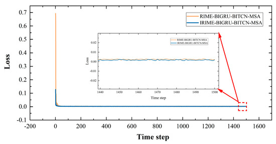
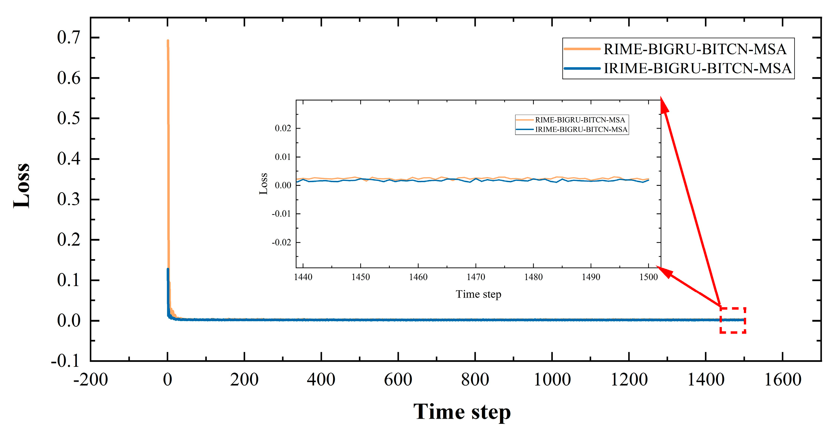
The loss plot illustrates the variation in loss values over time during the training process, providing researchers with an intuitive understanding of model learning efficiency and overfitting risk. By analyzing the loss plot, insights into the model’s performance on the training dataset can be gained. A decreasing loss value indicates that the model is continuously improving its ability to predict future industrial steam quantity. The loss plot is depicted in Figure 13.

Figure 13. Comparative model training loss graph.

This figure uses the number of training iterations as the x-axis and loss value as the y-axis, separately showcasing the performance of two optimization algorithms. The curve corresponding to the IRIME is consistently lower than that of the traditional RIME throughout the entire training process, particularly in the later stages of training. This indicates that the improved algorithm can more effectively reduce the model’s loss values, thereby enhancing prediction accuracy. Compared to the traditional RIME, IRIME not only accelerates the training process but also achieves significant reductions in loss values. This directly reflects the improvement in predictive accuracy of the improved model.

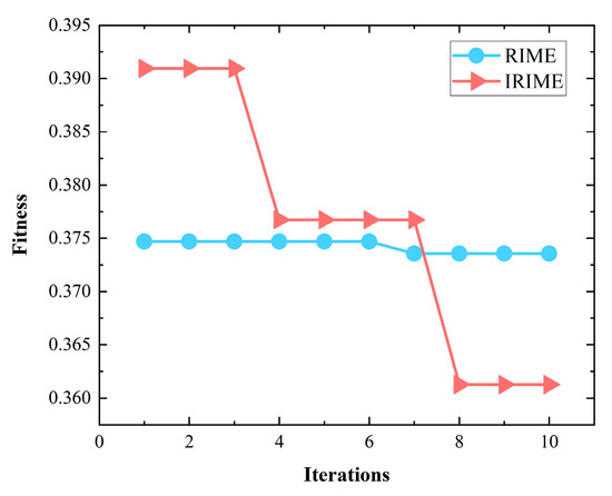
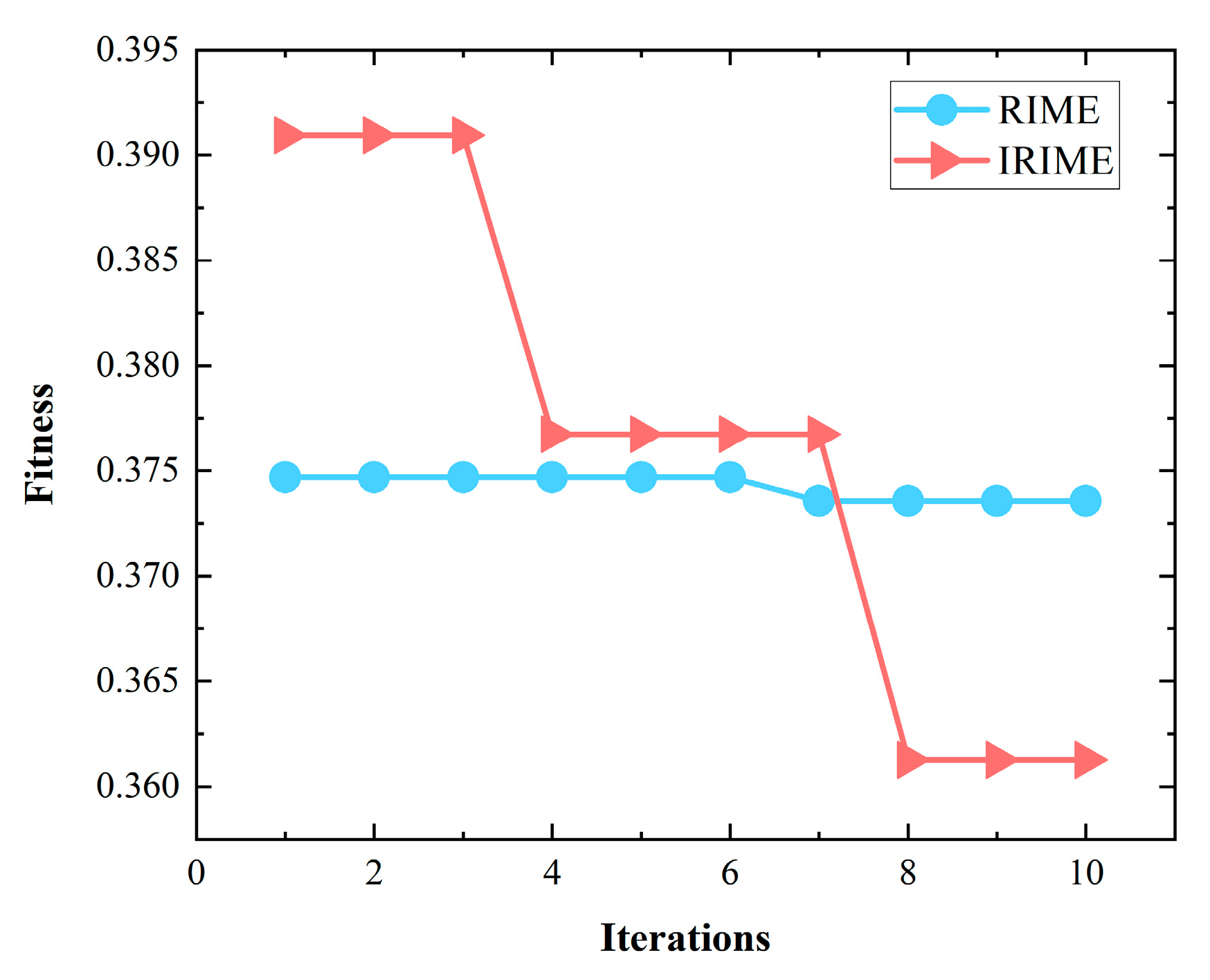
Figure 14 depicts that the curve corresponding to the IRIME converges more rapidly to lower loss values compared to the curve of the RIME. Particularly in the middle to later stages of training, the IRIME shows significantly faster convergence speed. This indicates that IRIME can effectively adjust model parameters during the optimization process to adapt to the training data.

Figure 14. Comparison graph of RIME model convergence values before and after improvement.

From Table 7, it is evident that IRIME-BiTCN-BiGRU-MSA shows improvements in all evaluation metrics compared to RIME-BiTCN-BiGRU-MSA. Specifically, R² increases from 0.84778 to 0.87966, indicating an improvement in the model’s goodness of fit to the data. MAE decreases from 0.28794 to 0.25114, RMSE decreases from 0.38383 to 0.34127, and MAPE decreases from 1.3146 to 1.2178. The reduction in these three metrics indicates an enhancement in prediction accuracy. RE decreases from 36.72% to 32.02%, indicating an improvement in prediction efficiency.

Table 7. Comparison results of evaluation metrics.

Method	R2	MAE	RMSE	MAPE	RE
RIME-BiTCN-BiGRU-MSA	0.84778	0.28794	0.38383	1.3146	36.72%
IRIME-BiTCN-BiGRU-MSA	0.87966	0.25114	0.34127	1.2178	32.02%

In summary, these results validate the effectiveness of the RIME and its improved version, IRIME. The improvements observed in key performance indicators demonstrate significant enhancements in accuracy, goodness of fit, and prediction efficiency with the IRIME.

5.5. Ablation Study

In study, ablation experiments are considered a crucial method for gaining deeper insights into the contributions of individual model components to prediction accuracy. By systematically removing or modifying different parts of the model, the impact of each component can be quantitatively evaluated, revealing the most critical factors affecting prediction outcomes. This approach not only enhances the interpretability of the model but also helps guide further optimization efforts. Subsequently, by comparing the performance of models under different configurations, including BiGRU, BiTCN-BiGRU, and their variants, the results of the ablation experiments are presented to gain a deeper understanding of the roles and importance of each component.

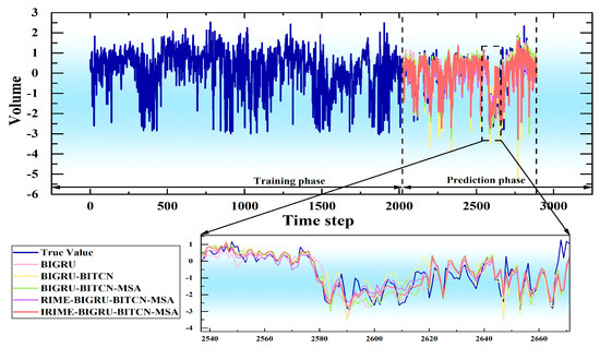
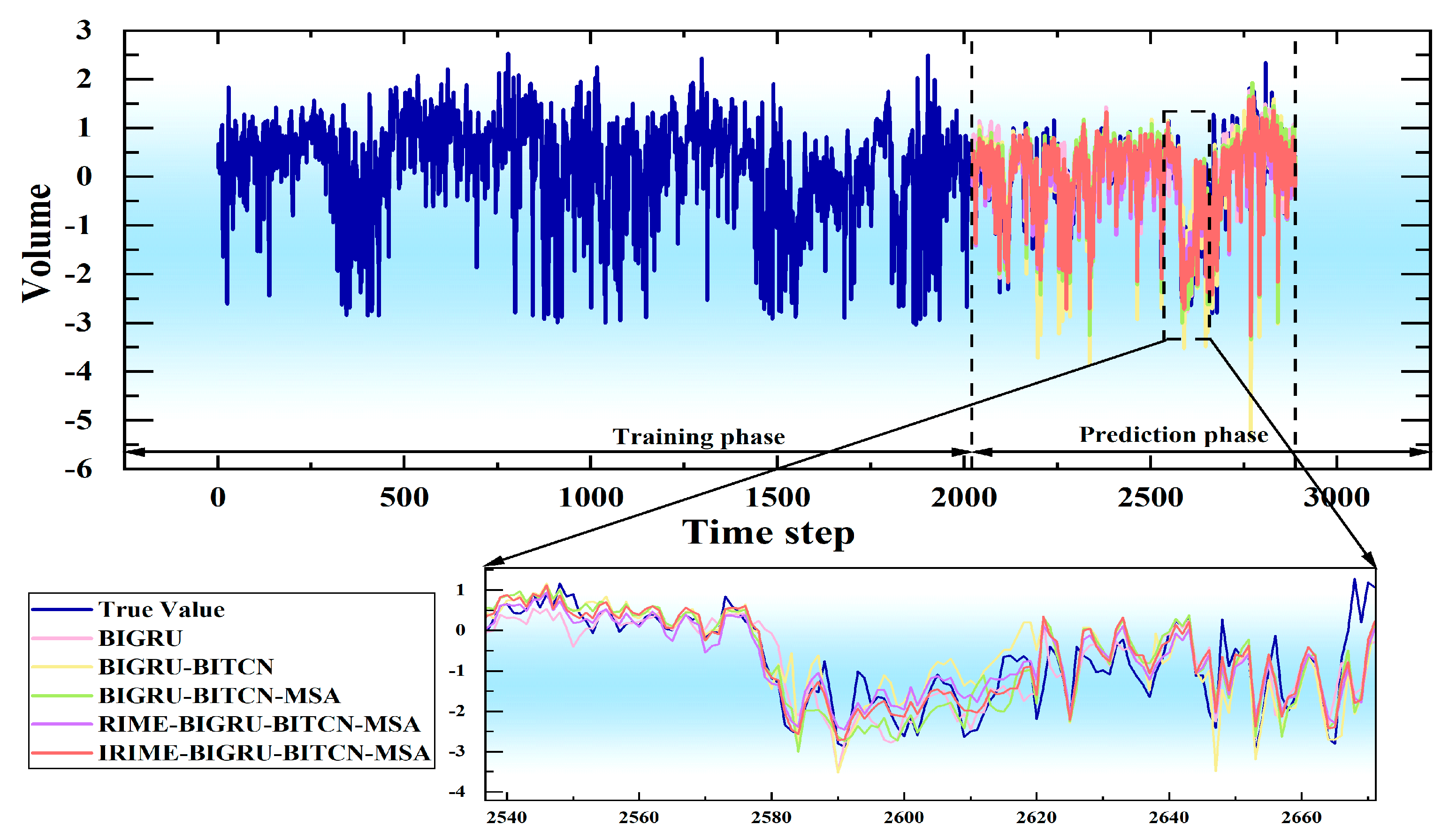
In order to visually assess the prediction accuracy of the IRIME-BiTCN-BiGRU-MSA method, Figure 15 compares the prediction results of this method with BiGRU, BiTCN-BiGRU, BiTCN-BiGRU-MSA, and RIME-BiTCN-BiGRU-MSA on the test set. It can be observed that the prediction results of IRIME-BiTCN-BiGRU-MSA (red) are relatively close to the true value (deep blue), with small deviations and very close curves, indicating that the improved model has good prediction performance.

Figure 15. Model ablation test fitting.

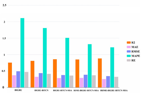
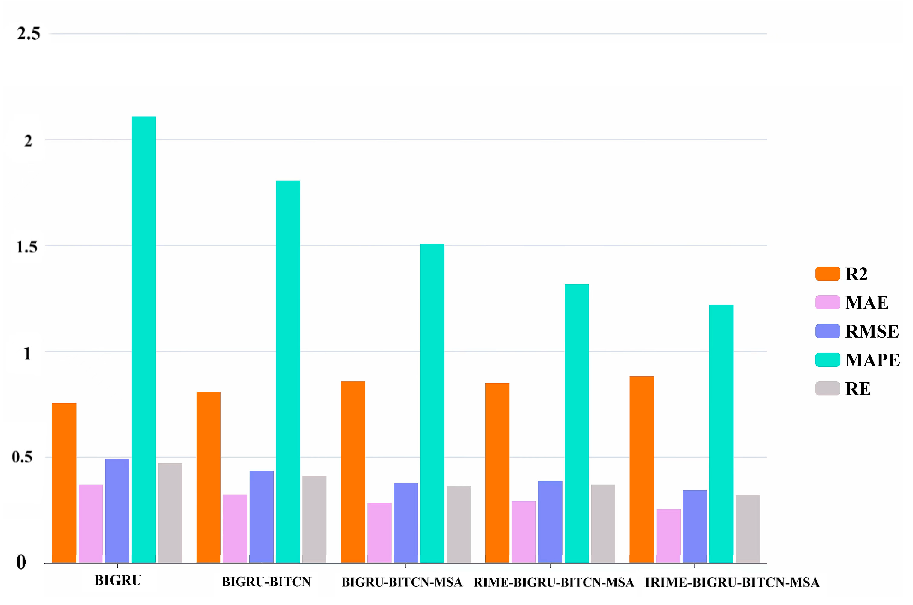
Table 8 and Figure 16 demonstrate that the IRIME-BiTCN-BiGRU-MSA model achieved an R² of 0.87966, MAE of 0.25114, RMSE of 0.34127, MAPE of 1.2178, and RE of 32.02%, significantly improving the performance over BiGRU. These enhancements highlight the effectiveness of BiTCN for capturing long-range dependencies, the multi-head self-attention mechanism for modeling complex relationships, and the IRIME technique for optimizing hyperparameters, resulting in a more robust and high-performing model.

Table 8. Summary of evaluation metric statistics.

Method	R2	MAE	RMSE	MAPE	RE
BiGRU	0.75288	0.36741	0.48905	2.108	46.85%
BiTCN-BiGRU	0.80598	0.32094	0.43334	1.8052	40.92%
BiTCN-BiGRU-MSA	0.85509	0.28128	0.3745	1.5066	35.87%
RIME-BiTCN-BiGRU-MSA	0.84778	0.28794	0.38383	1.3146	36.72%
IRIME-BiTCN-BiGRU-MSA	0.87966	0.25114	0.34127	1.2178	32.02%

Figure 16. Model ablation evaluation metrics comparison histogram.

5.6. Control Experiment

In this study, comparative experiments are crucial steps used to assess the performance and efficiency of different model structures. In this study, we compared our model with BiLSTM [44], CNN-BiGRU-SA [45], WOA-BiLSTM [46], and COA-CNN-LSTM [47]. These models are all recently published advanced methods, and comparing with them allows for a more comprehensive demonstration of the superior performance and effectiveness of the method proposed in this study for handling complex prediction tasks. The specific parameters are shown in Table 9.

Table 9. Initial parameter settings of comparative methods.

Algorithm Name	Parameter Initial	Configuration
BiLSTM CNN-BiGRU-SA WOA-BILSTM COA-CNN-LSTM	Learning Rate	0.0001
	Number of Neurons	10
	Number of Filters	20
	Regularization Parameter	0.00001
	Gradient Threshold	1
	Optimizer	Adam
	Max Training Iterations	100
	Attention Heads	1
	Attention Keys	10
WOA COA	Learning Rate	3
	Number of Neurons	10

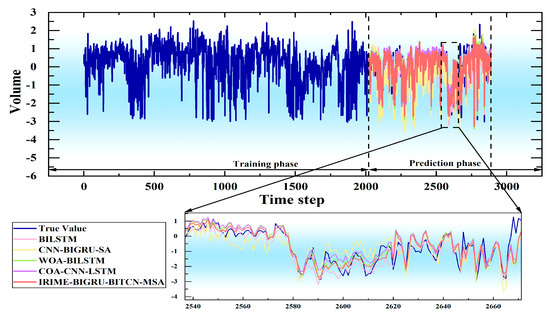
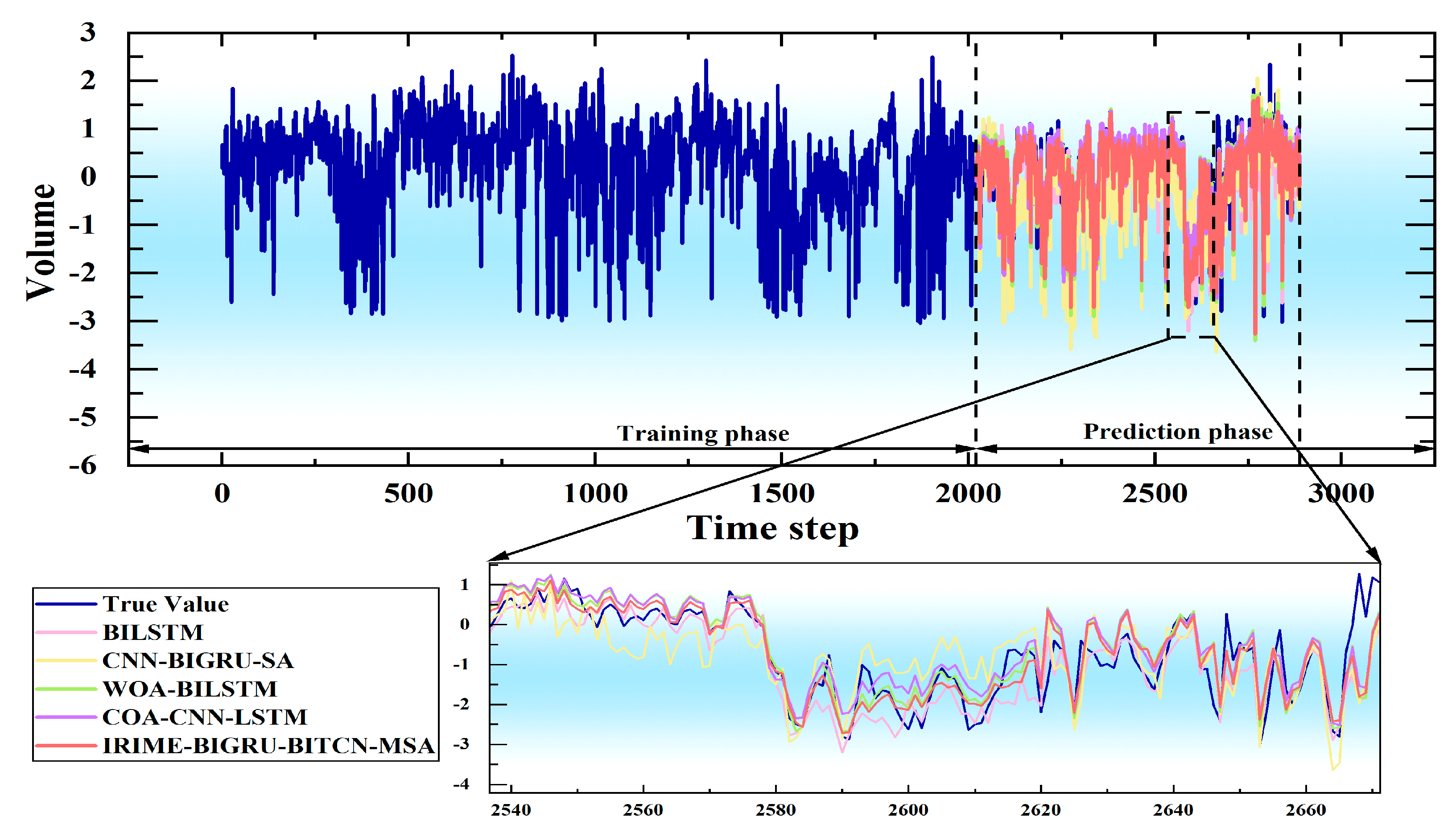
Figure 17 illustrates the comparison of prediction results between IRIME-BiTCN-BiGRU-MSA and BILSTM, CNN-BiGRU-SA, WOA-BILSTM, and COA-CNN-LSTM. It can be observed that the prediction results of IRIME-BiTCN-BiGRU-MSA (red) closely match the true value (dark blue), with relatively smaller deviations compared to other methods. This indicates that our model achieves higher prediction accuracy.

Figure 17. Model comparison test fitting.

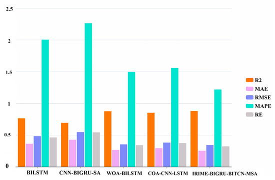
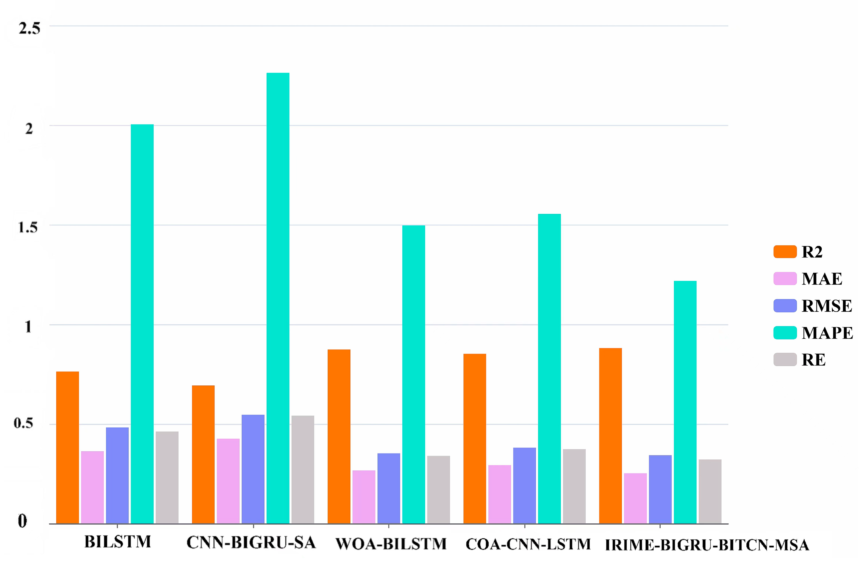
Table 10 and Figure 18 clearly show that the IRIME-BiTCN-BiGRU-MSA model outperforms other models across nearly all metrics. This includes the traditional BILSTM, the CNN-BiGRU-SA model, which combines convolutional neural networks and self-attention mechanisms, as well as the WOA-BILSTM and COA-CNN-LSTM models enhanced by optimization algorithms. Specifically, the IRIME-BiTCN-BiGRU-MSA model achieves an R² of 0.87966, an MAE of 0.25114, an RMSE of 0.34127, a MAPE of 1.2178, and an RE of 32.02%. These experimental results further prove the effectiveness and progressiveness of our model design.

Table 10. Summary of evaluation metrics.

Method	R2	MAE	RMSE	MAPE	RE
BILSTM	0.76182	0.36069	0.48013	2.0049	45.99%
CNN-BiGRU-SA	0.69217	0.42439	0.54583	2.2639	54.12%
WOA-BILSTM	0.87264	0.26515	0.35109	1.4974	33.81%
COA-CNN-LSTM	0.85109	0.2915	0.37964	1.5543	37.17%
IRIME-BiTCN-BiGRU-MSA	0.87966	0.25114	0.34127	1.2178	32.02%

Figure 18. Histogram comparing algorithm evaluation metrics.

6. Conclusions

This research successfully developed an efficient and accurate deep learning prediction model, the IRIME-BiTCN-BiGRU-MSA model. Initially, the model employed BiGRU to handle time-series data, but BiGRU faced challenges with long-term dependencies, often leading to gradient vanishing problems. To address this, BiTCN was introduced, improving the model’s ability to capture long-range dependencies by leveraging convolutional operations, thus mitigating the gradient vanishing issue. However, while BiTCN enhanced temporal feature extraction, it still struggled with capturing complex nonlinear relationships within the data. To overcome this, the multi-head self-attention mechanism was incorporated, enabling the model to globally compute data correlations and better capture intricate relationships. Despite these improvements, the model still faced challenges with optimizing hyperparameters effectively. By combining deep learning techniques with optimization algorithms, the IRIME technique was introduced to optimize hyperparameters, leading to a more robust and high-performing model. Through extensive testing on real datasets, the model demonstrated significant advantages across multiple key performance indicators, achieving an R² of 0.87966, MAE of 0.25114, RMSE of 0.34127, MAPE of 1.2178, and RE of 32.02%, surpassing other deep learning prediction models. This research not only improves the accuracy of industrial steam consumption prediction but also provides valuable insights and references for further research and practical applications of deep learning in the industrial domain. By accurately predicting steam demand, engineers can effectively manage energy usage, optimize production processes, reduce energy costs, and mitigate environmental impacts, thereby promoting sustainable industrial production.

Looking ahead, this research envisions that these efforts in model optimization, advanced data processing, and feature engineering, along with interdisciplinary applications, enhanced model interpretability, and the development of real-time prediction systems, will significantly improve the performance of industrial steam consumption prediction models. Specifically, by incorporating more sophisticated deep learning techniques and optimizing data processing workflows, the models’ accuracy and generalization capabilities are expected to undergo substantial enhancements. Moreover, extending the model’s application to other sectors such as electricity demand forecasting and water resource management will not only validate its universality and robustness but also contribute to broader sustainability goals. By integrating these models into real-time monitoring systems, instantaneous prediction and adjustment can be achieved, driving real-time optimization and boosting production efficiency. These advancements are expected to accelerate progress in the field of industrial steam consumption prediction, while also offering valuable insights for promoting sustainability through the wider application of deep learning technologies across various industrial sectors.

References

- Suganthi, L.; Samuel, A.A. Energy models for demand forecasting—A review. Renew. Sustain. Energy Rev. 2012, 16, 1223–1240. [Google Scholar] [CrossRef] [Scilit]
- Ahmad, T.; Chen, H.; Guo, Y.; Wang, J. A comprehensive overview on the data driven and large scale based approaches for forecasting of building energy demand: A review. Energy Build. 2018, 165, 301–320. [Google Scholar] [CrossRef] [Scilit]
- Sourcebook, A. Improving Steam System Performance: A Sourcebook for Industry; Elsevier: Amsterdam, The Netherlands, 2004. [Google Scholar]
- Bütün, H.; Kantor, I.; Maréchal, F. Incorporating location aspects in process integration methodology. Energies 2019, 12, 3338. [Google Scholar] [CrossRef] [Scilit]
- Wu, Y.; Wang, R.; Wang, Y.; Feng, X. An area-wide layout design method considering piecewise steam piping and energy loss. Chem. Eng. Res. Des. 2018, 138, 405–417. [Google Scholar] [CrossRef] [Scilit]
- Wu, Y.K.; Hong, J.S. A literature review of wind forecasting technology in the world. In Proceedings of the 2007 IEEE Lausanne Power Tech, Lausanne, Switzerland, 1–5 July 2007; pp. 504–509. [Google Scholar]
- Rahman, M.N.; Esmailpour, A. An efficient electricity generation forecasting system using artificial neural network approach with big data. In Proceedings of the 2015 IEEE First International Conference on Big Data Computing Service and Applications 2015, Redwood City, CA, USA, 30 March–2 April 2015; IEEE: Piscataway, NJ, USA, 2015; pp. 213–217. [Google Scholar]
- Çakir, U.; Comakli, K.; Yüksel, F. The role of cogeneration systems in sustainability of energy. Energy Convers. Manag. 2012, 63, 196–202. [Google Scholar] [CrossRef] [Scilit]
- Abusoglu, A.; Kanoglu, M. Exergetic and thermoeconomic analyses of diesel engine powered cogeneration: Part 1-Formulations. Appl. Therm. Eng. 2009, 29, 234–241. [Google Scholar] [CrossRef] [Scilit]
- Onat, N.; Bayar, H. The sustainability indicators of power production systems. Renew. Sustain. Energy Rev. 2010, 14, 3108–3115. [Google Scholar] [CrossRef] [Scilit]
- Kanoglu, M.; Dincer, I. Performance assessment of cogeneration plants. Energy Convers. Manag. 2009, 50, 76–81. [Google Scholar] [CrossRef] [Scilit]
- Hanus, K.; Variny, M.; Illés, P. Assessment and prediction of complex industrial steam network operation by combined thermo-hydrodynamic modeling. Processes 2020, 8, 622. [Google Scholar] [CrossRef] [Scilit]
- Hu, Y.; Man, Y. Energy consumption and carbon emissions forecasting for industrial processes: Status, challenges and perspectives. Renew. Sustain. Energy Rev. 2023, 182, 113405. [Google Scholar] [CrossRef] [Scilit]
- Dettori, S.; Matino, I.; Colla, V.; Speets, R. A Deep Learning-based approach for forecasting off-gas production and consumption in the blast furnace. Neural Comput. Appl. 2022, 34, 911–923. [Google Scholar] [CrossRef] [Scilit] [PubMed]
- Lin, Y.F.; Huang, T.M.; Chung, W.H.; Ueng, Y.L. Forecasting fluctuations in the financial index using a recurrent neural network based on price features. IEEE Trans. Emerg. Top. Comput. Intell. 2020, 5, 780–791. [Google Scholar] [CrossRef] [Scilit]
- Fang, X.; Zhang, W.; Guo, Y.; Wang, J.; Wang, M.; Li, S. A novel reinforced deep RNN-LSTM algorithm: Energy management forecasting case study. IEEE Trans. Ind. Inform. 2021, 18, 5698–5704. [Google Scholar] [CrossRef] [Scilit]
- Xia, M.; Shao, H.; Ma, X.; De Silva, C.W. A stacked GRU-RNN-based approach for predicting renewable energy and electricity load for smart grid operation. IEEE Trans. Ind. Inform. 2021, 17, 7050–7059. [Google Scholar] [CrossRef] [Scilit]
- Dai, Y.; Yu, W.; Leng, M. A hybrid ensemble optimized BiGRU method for short-term photovoltaic generation forecasting. Energy 2024, 299, 131458. [Google Scholar] [CrossRef] [Scilit]
- Jia, X.; Sang, Y.; Li, Y.; Du, W.; Zhang, G. Short-term forecasting for supercharged boiler safety performance based on advanced data-driven modelling framework. Energy 2022, 239, 122449. [Google Scholar] [CrossRef] [Scilit]
- Fakir, K.; Ennawaoui, C.; El Mouden, M. Deep Learning Algorithms to Predict Output Electrical Power of an Industrial Steam Turbine. Appl. Syst. Innov. 2022, 5, 123. [Google Scholar] [CrossRef] [Scilit]
- Peng, H.; Jiang, B.; Mao, Z.; Liu, S. Local enhancing transformer with temporal convolutional attention mechanism for bearings remaining useful life prediction. IEEE Trans. Instrum. Meas. 2023, 72, 1–12. [Google Scholar] [CrossRef] [Scilit]
- Zhang, L.; Wu, N.; Han, S.; Xiao, J.; Ruan, S. Electric vehicle battery swapping demand prediction based on feature selection and bidirectional temporal convolutional network. In Proceedings of the 2023 IEEE International Conference on Energy Internet (ICEI) 2023, Shenyang, China, 24–26 November 2023; pp. 340–345. [Google Scholar]
- Shi, T.; Li, P.; Yang, W.; Qi, A.; Qiao, J. Application of TCN-biGRU neural network in PM 2.5 concentration prediction. Environ. Sci. Pollut. Res. 2023, 30, 119506–119517. [Google Scholar] [CrossRef] [Scilit]
- Vaswani, A.; Shazeer, N.; Parmar, N.; Uszkoreit, J.; Jones, L.; Gomez, A.N.; Kaiser, L.; Polosukhin, I. Attention is all you need. Advances in Neural Information Processing Systems. arXiv 2017, arXiv:1706.03762. [Google Scholar]
- Ma, X.; Zheng, B.; Jiang, G.; Liu, L. Cellular Network Traffic Prediction Based on Correlation ConvLSTM and Self-Attention Network. IEEE Commun. Lett. 2023, 27, 1909–1912. [Google Scholar] [CrossRef] [Scilit]
- Bi, J.; Ma, H.; Yuan, H.; Zhang, J. Accurate prediction of workloads and resources with multi-head attention and hybrid LSTM for cloud data centers. IEEE Trans. Sustain. Comput. 2023, 8, 375–384. [Google Scholar] [CrossRef] [Scilit]
- Zhang, Y.M.; Wang, H. Multi-head attention-based probabilistic CNN-BiLSTM for day-ahead wind speed forecasting. Energy 2023, 278, 127865. [Google Scholar] [CrossRef] [Scilit]
- Gülmez, B. Stock price prediction with optimized deep LSTM network with artificial rabbits optimization algorithm. Expert Syst. Appl. 2023, 227, 120346. [Google Scholar] [CrossRef] [Scilit]
- Wang, K.; Hua, Y.; Huang, L.; Guo, X.; Liu, X.; Ma, Z.; Ma, R.; Jiang, X. A novel GA-LSTM-based prediction method of ship energy usage based on the characteristics analysis of operational data. Energy 2023, 282, 128910. [Google Scholar] [CrossRef] [Scilit]
- Guo, J.; Chen, C.; Wen, H.; Cai, G.; Liu, Y. Prediction model of goaf coal temperature based on PSO-GRU deep neural network. Case Stud. Therm. Eng. 2024, 53, 103813. [Google Scholar] [CrossRef] [Scilit]
- Li, G.; Wang, Y.; Xu, C.; Wang, J.; Fang, X.; Xiong, C. BO-STA-LSTM: Building energy prediction based on a Bayesian optimized spatial-temporal attention enhanced LSTM method. Dev. Built Environ. 2024, 18, 100465. [Google Scholar] [CrossRef] [Scilit]
- Naheliya, B.; Redhu, P.; Kumar, K. MFOA-Bi-LSTM: An optimized bidirectional long short-term memory model for short-term traffic flow prediction. Phys. A Stat. Mech. Its Appl. 2024, 634, 129448. [Google Scholar] [CrossRef] [Scilit]
- She, D.; Jia, M. A BiGRU method for remaining useful life prediction of machinery. Measurement 2021, 167, 108277. [Google Scholar] [CrossRef] [Scilit]
- Zhang, D.; Chen, B.; Zhu, H.; Goh, H.H.; Dong, Y.; Wu, T. Short-term wind power prediction based on two-layer decomposition and BiTCN-BiLSTM-attention model. Energy 2023, 285, 128762. [Google Scholar] [CrossRef] [Scilit]
- Ru, Y.; An, G.; Wei, Z.; Chen, H. Epilepsy detection based on multi-head self-attention mechanism. PLoS ONE 2024, 19, e0305166. [Google Scholar] [CrossRef] [Scilit] [PubMed]
- Li, X.; Wei, Z.; Lyu, Z.; Yuan, X.; Xu, J.; Zhang, Z. Federated Reinforcement Learning Based on Multi-head Attention Mechanism for Vehicle Edge Caching. In International Conference on Wireless Algorithms, Systems, and Applications; Springer: Cham, Switzerland, 2022; pp. 648–656. [Google Scholar]
- Su, H.; Zhao, D.; Heidari, A.A.; Liu, L.; Zhang, X.; Mafarja, M.; Chen, H. RIME: A physics-based optimization. Neurocomputing 2023, 532, 183–214. [Google Scholar] [CrossRef] [Scilit]
- Liu, S.; Jin, Z.; Lin, H.; Lu, H. An improve crested porcupine algorithm for UAV delivery path planning in challenging environments. Sci. Rep. 2024, 14, 20445. [Google Scholar] [CrossRef] [Scilit] [PubMed]
- Trojovský, P.; Dehghani, M. Subtraction-average-based optimizer: A new swarm-inspired metaheuristic algorithm for solving optimization problems. Biomimetics 2023, 8, 149. [Google Scholar] [CrossRef] [Scilit] [PubMed]
- Rugema, F.X.; Yan, G.; Mugemanyi, S.; Jia, Q.; Zhang, S.; Bananeza, C. A cauchy-Gaussian quantum-behaved bat algorithm applied to solve the economic load dispatch problem. IEEE Access 2020, 9, 3207–3228. [Google Scholar] [CrossRef]
- Mirjalili, S.; Mirjalili, S.M.; Lewis, A. Grey wolf optimizer. Adv. Eng. Softw. 2014, 69, 46–61. [Google Scholar] [CrossRef] [Scilit]
- Wang, D.; Tan, D.; Liu, L. Particle swarm optimization algorithm: An overview. Soft Comput. 2018, 22, 387–408. [Google Scholar] [CrossRef] [Scilit]
- Meraihi, Y.; Ramdane-Cherif, A.; Acheli, D.; Mahseur, M. Dragonfly algorithm: A comprehensive review and applications. Neural Comput. Appl. 2020, 32, 16625–16646. [Google Scholar] [CrossRef] [Scilit]
- Guo, Y.; Li, Y.; Qiao, X.; Zhang, Z.; Zhou, W.; Mei, Y.; Lin, J.; Zhou, Y.; Nakanishi, Y. BiLSTM multitask learning-based combined load forecasting considering the loads coupling relationship for multienergy system. IEEE Trans. Smart Grid 2022, 13, 3481–3492. [Google Scholar] [CrossRef] [Scilit]
- Zhou, G.; Guo, Z.; Sun, S.; Jin, Q. A CNN-BiGRU-AM neural network for AI applications in shale oil production prediction. Appl. Energy 2023, 344, 121249. [Google Scholar] [CrossRef] [Scilit]
- Song, Y.; Xie, H.; Zhu, Z.; Ji, R. Predicting energy consumption of chiller plant using WOA-BiLSTM hybrid prediction model: A case study for a hospital building. Energy Build. 2023, 300, 113642. [Google Scholar] [CrossRef] [Scilit]
- Abou Houran, M.; Bukhari, S.M.S.; Zafar, M.H.; Mansoor, M.; Chen, W. COA-CNN-LSTM: Coati optimization algorithm-based hybrid deep learning model for PV/wind power forecasting in smart grid applications. Appl. Energy 2023, 349, 121638. [Google Scholar] [CrossRef] [Scilit]
Disclaimer/Publisher’s Note: The statements, opinions and data contained in all publications are solely those of the individual author(s) and contributor(s) and not of MDPI and/or the editor(s). MDPI and/or the editor(s) disclaim responsibility for any injury to people or property resulting from any ideas, methods, instructions or products referred to in the content. |
© 2024 by the authors. Licensee MDPI, Basel, Switzerland. This article is an open access article distributed under the terms and conditions of the Creative Commons Attribution (CC BY) license (https://creativecommons.org/licenses/by/4.0/).