Explainable LightGBM of Plant-Growth Responses Across Diverse LED Experiments

Abstract

Interpreting plant-growth responses across diverse light-emitting diode (LED) experiments requires attention to differences in species, lighting conditions, measurements, and experimental design. This study combines a descriptive comparison of six public LED-growth resources with an explainable Light Gradient Boosting Machine (LightGBM 4.6.0) case study. The resources cover sweet pepper, lettuce, soybean, Arabidopsis, European yew, and ornamental plants; regression modeling and SHapley Additive exPlanations (SHAP 0.50.0) analysis were conducted only on sweet pepper. Of 144 original observations, 71 complete records were retained for dry-biomass prediction. On the original held-out test set, LightGBM Model A outperformed ridge regression (R² = 0.755 versus 0.460; RMSE = 0.136 versus 0.216 g; MAE = 0.104 versus 0.185 g). However, leave-one-temporal-replicate-out cross-validation favored ridge regression (mean R² = 0.600 ± 0.191) over LightGBM (0.078 ± 0.248). Excluding instrument gain and additional harvest-related predictors reduced LightGBM R² to 0.111. SHAP ranked chlorophyll-fluorimeter gain and LED treatment highest in Model A, whereas LED treatment and initial plant height led Model B. The resource comparison identifies challenges in comparing lighting treatments and growth measurements, while the case study demonstrates sensitivity to predictor availability and validation design. Together, these findings clarify the requirements for applying explainable LightGBM to diverse LED experiments without establishing cross-species predictive generalizability or causal lighting effects.

1. Introduction and Justification of Study

Light is a central environmental variable in controlled plant production because its duration, intensity, and spectral composition influence photosynthesis, morphology, development, biomass allocation, and quality. Tunable light-emitting diode (LED) systems permit precise adjustment of these properties across greenhouse, indoor-farm, growth-chamber, propagation, and speed-breeding applications [1]. Extensive photobiological research has documented how plants respond to different regions of the light spectrum, with red, blue, green, and far-red wavelengths associated with distinct physiological and developmental responses [2]. Red and far-red light are primarily perceived by phytochromes, which regulate plant development, stem elongation, and shade-avoidance responses. Blue light is detected by cryptochromes and phototropins, which influence stomatal opening, chloroplast movement, and photomorphogenesis. Photoreceptor signaling also interacts with endogenous hormones to regulate elongation. In Arabidopsis, blue-light-activated CRY1 interacts with GID1 and DELLA proteins, inhibits gibberellin-induced DELLA degradation, and thereby restrains hypocotyl elongation [3]. This provides a mechanistic example of how light perception can modify growth through hormone signaling; the pathway was not measured in the present sweet-pepper analysis. Furthermore, different LED wavelengths influence chlorophyll biosynthesis and photosynthetic performance, contributing to variations in plant growth and biomass accumulation [4]. In addition to spectral quality, photoperiod and light intensity play key roles in shaping growth trajectories and biomass outcomes [5]. These lighting factors rarely act independently; instead, plant responses emerge from complex and nonlinear interactions among multiple light parameters.

As LED systems become increasingly tunable, experiments involve combinations of spectral composition, intensity, and temporal regimes [6]. Statistical models can represent such effects through specified terms and interactions, whereas tree-based machine learning offers a flexible approach to learning nonlinear relationships. LightGBM is an efficient implementation of gradient-boosted decision trees [7]. It has been applied to agricultural data together with explainability methods [8]. The value of this approach depends on the dataset and validation design, particularly when sample sizes are small [9].

Despite their predictive power, machine learning models are often criticized for limited interpretability, which can hinder their acceptance in plant science and horticultural research [10]. Explainable artificial intelligence (XAI) methods address this limitation by providing transparent insights into how models generate predictions. SHapley Additive exPlanations (SHAPs) offer a principled framework for quantifying the contribution of individual input features to model outputs [11,12]. SHAP has been applied in agricultural contexts including soil analysis, irrigation assessment, disease detection, and yield prediction, enabling researchers to interpret model behavior and assess feature importance in a transparent manner [13,14,15,16]. In the context of plant growth modeling, SHAP can be used to identify which experimental variables most strongly influence predicted outcomes and to evaluate the stability of these influences across different modeling conditions [17].

Previous research has examined plant responses to LED treatments [4], while a related study used logistic regression and SHAP for LED-based plant-growth analysis [18]. The present study examines the comparability of diverse LED-growth resources and uses continuous biomass prediction to investigate LightGBM feature attribution and validation sensitivity. This connects the broader challenge of interpreting heterogeneous LED experiments with a focused empirical analysis, without assuming that explanatory patterns from one experiment transfer to other species or conditions.

The study has two complementary components: a descriptive comparison across six diverse LED experiments and a LightGBM–SHAP case study using sweet-pepper dry biomass. The objectives were to (i) characterize differences in plant material, lighting conditions, measurements, and experimental structure across the six resources; (ii) evaluate LightGBM biomass prediction against a ridge-regression benchmark within sweet pepper; (iii) identify influential predictors using SHAP; and (iv) examine how feature exclusion and grouped validation affect interpretation. The cross-experiment component concerns dataset comparability, whereas all fitted models, performance metrics, and SHAP attributions concern the sweet-pepper case study. This distinction defines the scope of the analysis across diverse experiments and avoids treating within-study associations as evidence of cross-species transfer or causal treatment effects.

2. Materials and Methods

2.1. Diverse LED Experiments and Scope of Analysis

Six public LED-growth resources were examined to compare plant material, lighting conditions, measurement scales, and experimental context [2,5,19,20,21,22]. They span food crops, a model species, ornamental seedlings, and a woody gymnosperm (Table 1), providing the descriptive basis for the comparison across diverse LED experiments. Sweet pepper supplied the data for the LightGBM–SHAP case study and ridge-regression benchmark. The other five resources were examined descriptively; no models were fitted to them, and no cross-species pooling or common unit conversion was performed.

Table 1. Diverse public LED-growth experiments examined for descriptive comparison. Sweet pepper supplied the data for the LightGBM–SHAP case study; the remaining resources were not used for model fitting or validation.

Dataset DOI	Plant Material	Lighting Contrast	Experimental Context
10.6084/m9.figshare.22299847	Sweet pepper (Capsicum annuum)	12 h baseline; white or red–blue extension	Greenhouse; insect/parasitoid treatments
10.6084/m9.figshare.27260871.v1	Lettuce (Lactuca sativa ‘Rex’ and ‘Rouxai’)	12 blue-green-red-far-red spectra	Indoor production; two temporal blocks
10.5061/dryad.rfj6q578c	Soybean (Glycine max; diverse maturity groups)	Red–blue versus full-spectrum white	Controlled speed-breeding environment
10.57745/ZCFBUT	Arabidopsis thaliana (four genotypes)	Six LED spectra plus neon control	Growth chambers; three biological replicates
10.1371/journal.pone.0266777.s003	European yew (Taxus baccata)	LED spectrum and intensity	Smart greenhouse; woody species
10.6084/m9.figshare.6946136	Begonia, geranium, petunia, and snapdragon	Six sole-source LED spectra	Controlled-environment ornamental seedlings

The source files examined contained 144 sweet-pepper records, 384 lettuce records (192 per cultivar), 1292 soybean worksheet records, 83 Arabidopsis records, 180 European-yew biometric records and 60 metabolomic records, and 122 rows in each of four ornamental-species worksheets. These are source-table counts, not necessarily numbers of independent experimental units, and the worksheets were not combined. For sweet pepper, complete-case selection retained 71 records and 15 Model A predictors; 73 records (50.7%) were excluded. Plant height was expressed in centimeters, dry biomass in grams, and Fv/Fm as a dimensionless ratio. Preprocessing removed incomplete records and explicit target or mass-component variables; Model B excluded further predictors as described in Section 2.2.

LED treatment identifiers were interpreted within their source experiments. Differences in spectral composition, light intensity, and photoperiod mean that similarly numbered treatments need not represent equivalent exposures. Consequently, LED treatment importance in the sweet-pepper model cannot be used to rank treatments in lettuce, soybean, Arabidopsis, European yew, or ornamental plants. The descriptive comparison identifies this limitation; it does not constitute numerical harmonization for pooled modeling.

Lighting conditions were compared by spectral composition, photon flux density, and daily lighting duration where these details were available. Sweet pepper received a 12 h white-light baseline, with either no extension or a 6 h white or red–blue extension [21]. Lettuce received twelve blue-green-red-far-red treatments at a target total photon flux density of approximately 176 μmol m⁻² s⁻¹ and a 20 h photoperiod; total photon flux includes far-red and is not interchangeable with conventional PPFD [5]. Ornamental seedlings received six mint-white, red, blue, and green combinations at PPFD 160 μmol m⁻² s⁻¹ for 18 h daily [22]. Soybean compared red–blue and full-spectrum lighting, Arabidopsis compared six LED spectra with a neon control, and European yew received supplemental greenhouse lighting [2,19,20]. A complete treatment-level inventory of spectra, photon flux densities, and photoperiods for all six resources is not established here. These descriptions therefore support contextual comparison, not numerical equivalence or pooled treatment coding.

For the sweet-pepper analysis, complete records were selected and feature sets were defined before model fitting. The same retained observations were used to compare models, and a fixed random seed was used for the original train–test split.

Table 2 defines the 15 predictors reported for Model A and the dry-biomass target. Predictors include LED treatment, structural growth measurements, chlorophyll fluorescence measurements, the fluorimeter gain setting, and experimental descriptors. Instrument gain is a measurement setting, not an indicator of biomass accumulation. Harvest block, temporal replicate, cage code, and insect treatment describe aspects of the experimental design. Their inclusion permits prediction within the observed data but does not establish their availability or usefulness in a new experiment.

Table 2. Feature definitions used in model development, including variable descriptions and their roles in the predictive pipeline.

Feature Name	Description	Role
LED Treatment	Encoded identifier representing the applied LED lighting treatment	Input
Chlorophyll-Fluorimeter Gain	Fluorimeter setting; not biomass gain	Input
Initial Plant Height (Day 16)	Plant height measured at the early growth stage (16 days after planting)	Input
Raw Final Plant Height	Final plant height measured at harvest (raw measurement)	Input
Corrected Final Plant Height	Final plant height after correction for measurement artifacts	Input
Plant Height Increase	Difference between final and initial plant height	Input
Leaf Number	Total number of leaves per plant	Input
Leaf Number (Excluding Aphid Sampling)	Leaf count excluding leaves sampled for aphid analysis	Input
Fv/Fm Ratio (Unscaled)	Raw maximum quantum efficiency of photosystem II (Fv/Fm)	Input
Fv/Fm Ratio (Scaled)	Scaled maximum quantum efficiency of photosystem II (Fv/Fm)	Input
Harvest Block	Source takedown-block identifier describing the harvest grouping	Input
Temporal Replicate	Identifier indicating the temporal replicate of the experiment	Input
Cage Code	Identifier of the experimental cage	Input
Insect Treatment	Indicator of insect treatment condition	Input
Fluorescence Leaf Position	Leaf position used for chlorophyll fluorescence measurement	Input
Total Dry Mass	Final plant dry biomass used as the prediction target	Target

Plant dry biomass was selected as the response variable because it provides a quantitative indicator of accumulated plant growth and organic matter production. Unlike fresh biomass, dry biomass is less directly influenced by differences in plant water content, making it useful for evaluating growth performance. However, differences in plant species, developmental stages, and growth characteristics may influence biomass accumulation and its interpretation. Therefore, dry biomass should be considered a general indicator of plant growth rather than a directly equivalent measure of physiological performance across all species.

2.2. Data Preprocessing and Leakage Control

Data preprocessing used complete-case selection and excluded variables representing fresh-mass or dry-mass components directly related to the total dry-mass target before model training.

Two LightGBM configurations were evaluated using the same retained observations. Model A included 15 predictors after exclusion of explicit target and mass-component variables. Model B retained six predictors from Model A, including LED treatment, initial plant height (day 16), harvest block, leaf number (total number of leaves per plant), temporal replicate, and insect treatment. These names follow the definitions in Table 2. The retained set combines treatment conditions, baseline plant size, leaf count, and experimental descriptors. Model B was evaluated as a reduced-feature sensitivity analysis after exclusion of instrument gain and selected other measurements.

The distinction between association and leakage depends on how and when a predictor was measured. A variable may correlate strongly with dry biomass without being derived from it, while a harvest-time measurement may be unavailable for early-stage prediction. Model B retains leaf number and harvest block; excluding instrument gain and other selected measurements therefore does not establish that all retained inputs are available before harvest. The analyses assess contemporaneous biomass estimation and feature sensitivity, rather than validated early-stage prediction.

The source variable gain represents the chlorophyll-fluorimeter instrument gain setting rather than biomass accumulation. Although it is not derived from total dry mass, it was correlated with the target (r = 0.760). Excluding gain reduced LightGBM R² from 0.755 to 0.562; excluding additional harvest-related predictors reduced R² to 0.111. These changes indicate dependence on measurement-related and harvest-time information.

2.3. Regression Models and Evaluation

LightGBM was used to model nonlinear relationships between the selected predictors and sweet-pepper dry biomass. Ridge regression provided a regularized linear benchmark. For the ridge-LightGBM benchmark, both algorithms used the same source predictors, target observations, and evaluation partitions.

The original held-out evaluation used 56 training observations and 15 test observations from the 71 retained records. Model A and Model B used the same observations, split, and LightGBM hyperparameters, allowing the effect of feature exclusion to be examined separately from changes in the test sample.

Predictive performance was assessed using the coefficient of determination (R²), root mean squared error (RMSE), and mean absolute error (MAE). R² is dimensionless; RMSE and MAE are expressed in grams. Metrics were calculated on the held-out test observations and, separately, on the validation observations in each grouped cross-validation fold.

Leave-one-temporal-replicate-out cross-validation evaluated transfer across four temporal replicates of the sweet-pepper experiment. In each of the four folds, one entire replicate was reserved for validation and the other three were used for training. Each validation fold contained approximately 17–18 observations, and no cage identifiers overlapped between training and validation sets. Ridge regression and LightGBM used the same source predictors and validation partitions.

2.4. SHAP Analysis

SHAP values were computed using TreeExplainer (specialized explainability algorithm within the open-source SHAP 0.50.0 library) for the same 56 training observations in both LightGBM configurations. Global feature importance was summarized by the mean absolute SHAP value for each feature. These values are expressed in grams, matching the dry-biomass prediction scale, and describe the fitted models on the training observations.

SHAP analysis was performed separately for Model A and Model B to assess changes in predictor ranking and contribution magnitude after feature exclusion. Attributions were interpreted as model-dependent associations, not causal effects or a test proving the absence of information leakage.

3. Experimental Results

3.1. Model Performance Evaluation

On the original held-out test set, LightGBM Model A achieved R² = 0.755, RMSE = 0.136 g, and MAE = 0.104 g, compared with R² = 0.460, RMSE = 0.216 g, and MAE = 0.185 g for ridge regression (Table 3). This comparison favors LightGBM for the selected test observations. The grouped cross-validation results below provide a separate assessment of transfer between temporal replicates.

Table 3. Held-out test performance of ridge regression and LightGBM Model A for sweet-pepper dry-biomass prediction.

Model	R2	RMSE (g)	MAE (g)
Ridge Regression	0.460	0.216	0.185
LightGBM Regression (Model A)	0.755	0.136	0.104

The held-out comparison evaluates predictions for observations in the selected split, whereas grouped cross-validation evaluates predictions for an entire temporal replicate excluded from training. Performance remains conditional on each algorithm’s preprocessing and parameter settings.

Using the same observations, train–test partition, and LightGBM hyperparameters, the reduced-feature Model B achieved R² = 0.111, RMSE = 0.259 g, and MAE = 0.197 g, compared with R² = 0.755, RMSE = 0.136 g, and MAE = 0.104 g for Model A. The decline after reducing the predictor set from 15 to six indicates sensitivity to the excluded information. Table 4 reports the mean and standard deviation (SD) of each metric across the four folds.

Table 4. Grouped cross-validation performance of ridge regression and LightGBM. Values are mean ± SD across four folds, each withholding one entire temporal replicate of the sweet-pepper experiment; individual fold scores are not reported.

Model	R2 (Mean ± SD)	RMSE (g; Mean ± SD)	MAE (g; Mean ± SD)
Ridge Regression	0.600 ± 0.191	0.098 ± 0.038	0.082 ± 0.028
LightGBM Regression	0.078 ± 0.248	0.155 ± 0.061	0.118 ± 0.045

Grouped cross-validation favored ridge regression over LightGBM: mean R² was 0.600 versus 0.078, mean RMSE was 0.098 versus 0.155 g, and mean MAE was 0.082 versus 0.118 g (Table 4). Ridge regression also had smaller across-fold standard deviations for all three metrics. The reversal of the original held-out ranking indicates that the apparent LightGBM advantage depends on the data partitioning strategy.

3.2. SHAP Global Feature Importance Analysis

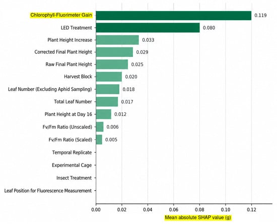
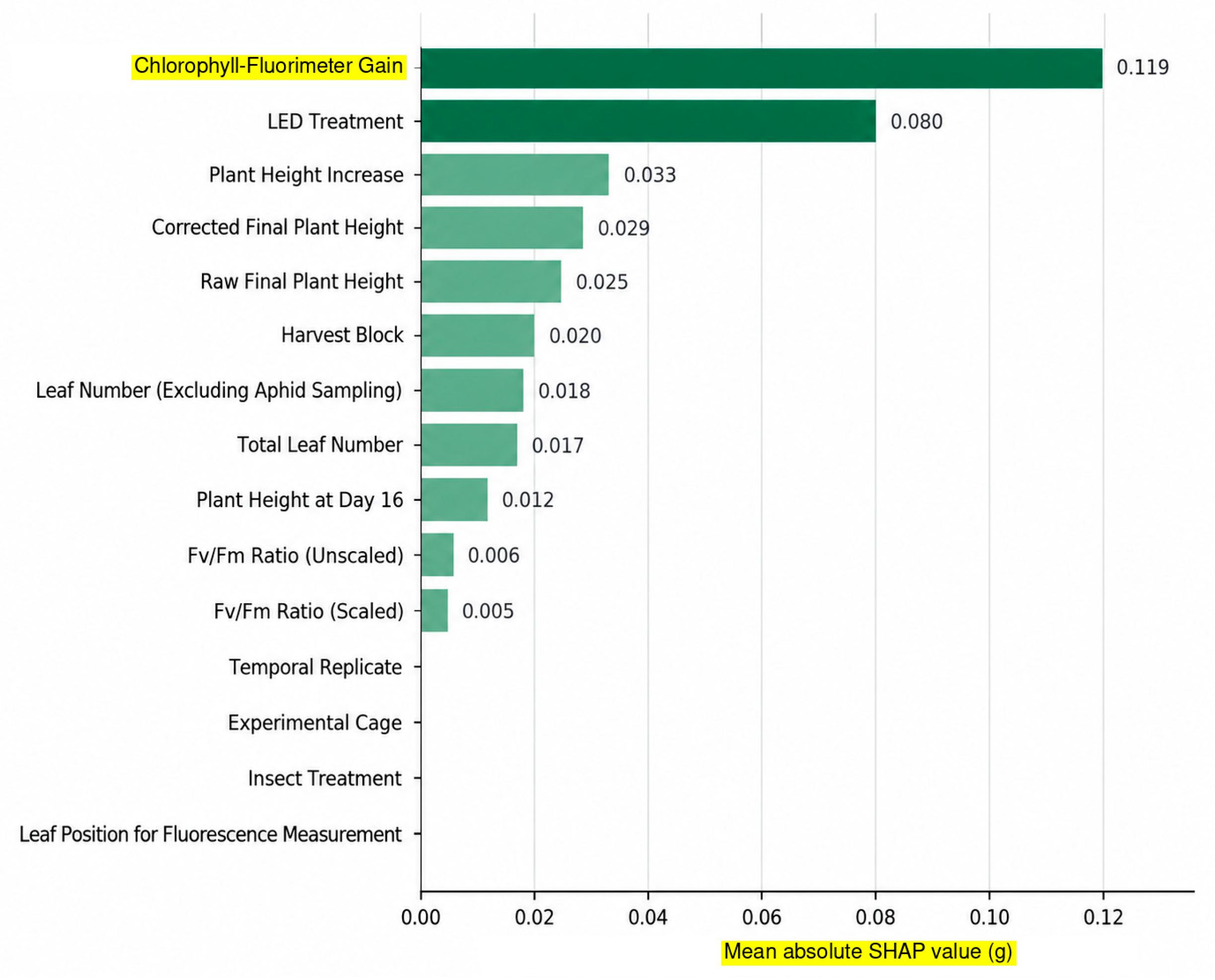
In Model A, chlorophyll-fluorimeter gain had the largest mean absolute SHAP value (0.119481 g), followed by LED treatment (0.080051 g), plant height increase (0.033137 g), corrected final plant height (0.029427 g), and raw final plant height (0.024537 g). Harvest block contributed approximately 0.020 g (Figure 1). Leaf number excluding aphid sampling (0.017892 g) and total leaf number (0.016609 g) contributed less, followed by initial plant height at day 16 (0.011934 g). Chlorophyll fluorescence variables had mean absolute SHAP values below 0.0061 g, while temporal replicate, cage code, insect treatment, and fluorescence leaf position had near-zero values.

Figure 1. Global feature importance for LightGBM Model A, expressed as mean absolute SHAP values (g) across 56 training observations. Mean absolute SHAP values represent the average magnitude of each feature’s contribution to predicted dry biomass relative to the model’s expected prediction. Values are expressed in grams because the model predicts dry biomass in grams. Larger values indicate greater average influence on predictions, without indicating whether the feature increases or decreases predicted biomass. Chlorophyll-fluorimeter gain denotes the instrument setting, not biomass gain. Harvest block corresponds to the source takedown-block variable. Descriptive feature labels are used consistently with Table 2 and Section 3.2.

The near-zero contributions of these experimental descriptors indicate limited reliance by the fitted model, not an absence of experimental or biological significance. Grouping may still affect generalization, as the cross-validation results demonstrate.

These global importance values summarize the magnitude of feature contributions across the training observations. They do not indicate the direction of a feature’s association with predicted biomass.

Model A relied most on the fluorimeter setting, treatment information, and structural measurements. Instrument gain is a measurement setting whose predictive contribution may be specific to the source instrument or experiment; it is not a measure of biomass accumulation.

SHAP values describe predictive contributions within the fitted model and do not establish causal relationships or biological mechanisms.

For Model B, the leading mean absolute SHAP values were LED treatment (0.119 g), initial plant height at day 16 (0.085 g), and harvest block (0.036 g). The comparison used the same 56 training observations and TreeExplainer method as Model A. LED treatment remained prominent in both models, but the leading predictors and contribution magnitudes changed. This shared predictor therefore does not establish overall ranking stability, particularly given Model B’s lower predictive accuracy.

3.3. LightGBM Model Configuration

The LightGBM configuration used for the reported regression analyses is summarized in Table 5. The same configuration was retained for Model A and Model B. Performance was assessed on held-out observations and through grouped cross-validation, as described in Section 2.3.

Table 5. LightGBM hyperparameter configuration and evaluation metrics used for biomass prediction.

Parameter	Value	Description
Number of Estimators	500	Number of boosting trees used in the model
Learning Rate	0.05	Step size controlling the contribution of each tree
Number of Leaves	31	Maximum number of leaves per decision tree
Subsample	0.8	Training-row sampling fraction; effective only when bagging is enabled
Column Sample by Tree	0.8	Fraction of features randomly selected for each tree
Random State	42	Fixed seed to ensure reproducibility
Categorical Features	Specified explicitly	Enables native handling of categorical variables by LightGBM
Objective	Regression	Predict continuous plant dry biomass
Evaluation Metrics	R2, RMSE, MAE	Metrics used to assess model performance

The row-sampling fraction in Table 5 takes effect only when bagging frequency is greater than zero.

4. Discussion

This study considers explainable LightGBM analysis in the context of diverse LED-growth experiments through a six-resource comparison and a sweet-pepper modeling case study. The comparison establishes differences in species, lighting contrasts, measurement scales, and experimental structure; the case study examines how these methodological concerns arise in a fitted biomass model. SHAP describes the contributions of measured variables to sweet-pepper predictions. It does not provide a common ranking of physiological responses across the six resources or establish causal lighting mechanisms.

Feature exclusion changed both predictive performance and SHAP importance. Instrument gain was the leading predictor in Model A, whereas LED treatment and initial plant height led Model B. The reduction in held-out R² from 0.755 to 0.111 indicates that Model A depended strongly on information excluded from Model B. These changes warrant caution when transferring the model to settings where harvest-time measurements or source-specific instrument settings are unavailable.

LED spectral composition can influence photosynthesis, morphology, and biomass accumulation [23]. However, the high SHAP importance of LED treatment here reflects its contribution to model predictions, not a statistical test of a lighting effect. Structural measurements such as plant height and leaf number also contribute predictive information. These associations depend on the experimental conditions and cannot be used to identify an optimal spectrum or establish a physiological mechanism.

Previous work has examined machine learning for crop prediction [24], including a LightGBM–SHAP framework [25]. In the present case study, LightGBM outperformed ridge regression on the original test split, but the ranking reversed under grouped cross-validation. Differences in datasets, experimental design, and validation procedures preclude direct comparison of performance across studies. The six-resource comparison provides context for these differences, while the quantitative contribution is the examination of predictive performance, feature sensitivity, and model attribution within sweet pepper.

Chlorophyll fluorescence (Fv/Fm) reflects the maximum quantum efficiency of photosystem II and is commonly used to assess plant photosynthetic performance and stress responses [26]. Its relatively low SHAP importance may indicate that Fv/Fm exhibited limited variation under the experimental conditions or that its predictive information overlapped with other growth-related variables. In contrast, LED treatment showed greater predictive importance, potentially reflecting differences in spectral composition, light intensity, and photoperiod that influence photosynthesis, plant morphology, and biomass accumulation [27]. However, the lower SHAP contribution of Fv/Fm does not imply that photosynthetic efficiency is physiologically unimportant, as SHAP values represent model-based predictive contributions rather than direct biological effects.

SHAP provides additive feature attributions for individual predictions [11], making model reliance more transparent. In this study, comparing explanations across feature sets exposed sensitivity to predictor selection. SHAP does not validate the experimental design, establish physiological causation, or rule out information leakage; those questions require examination of measurement timing, source definitions, and independent validation.

The grouped results suggest that the nonlinear relationships learned by LightGBM were sensitive to experimental variation and the small sample available for training. Ridge regression’s stronger performance across withheld temporal replicates supports the use of a simpler benchmark and shows why a single random split cannot establish generalizability.

Several limitations remain. Complete-case selection retained 71 of 144 original records, excluding 73 records (50.7%) and potentially changing the distribution of treatments or experimental groups. The small retained sample limits precision and model complexity. SHAP explanations were evaluated on training observations, and correlated predictors may share predictive information. The findings are restricted to the sweet-pepper experiment and cannot establish performance in other species, environments, or lighting regimes.

Leave-one-temporal replicate-out cross-validation provides an assessment of transfer within sweet pepper, but four folds offer only a limited estimate of variability. Table 4 summarizes the completed analysis as mean ± SD; individual fold scores are not presented. Future work will rerun grouped validation with systematic retention and reporting of each fold’s temporal-replicate identifier, training and validation sample sizes, and R², RMSE, and MAE for both algorithms. This will allow performance differences among replicates to be examined directly.

Taken together, the resource comparison and case study identify two requirements for interpreting plant-growth responses across diverse LED experiments: comparable definitions of predictors and outcomes, and validation that respects experimental grouping. The sweet-pepper analysis illustrates why feature availability and validation design matter for LightGBM–SHAP interpretation. Applying this approach to the other resources would require study-specific preprocessing and independent evaluation.

5. Conclusions

This study combines a descriptive comparison of six diverse LED-growth experiments with a LightGBM regression model interpreted using SHAP in a sweet-pepper case study. The comparison documents differences relevant to modeling plant-growth responses, while the case study quantifies how selected predictors contribute to dry-biomass predictions. Thus, the study addresses explainable LightGBM within a diverse experimental context while limiting quantitative inference to the experiment used for model fitting and evaluation.

Within the sweet-pepper case study, LightGBM performed better on the original test split, whereas ridge regression performed better when entire temporal replicates were held out. Instrument gain, LED treatment, and structural measurements were influential in Model A, but the reduced-feature configuration had substantially lower predictive accuracy. These results show that model interpretation depends on predictor availability and validation design.

The combined findings support careful use of LightGBM and SHAP to examine plant-growth prediction under LED lighting. The diversity of the six resources motivates explicit treatment definitions, measurement provenance, and experimental grouping, while the sweet-pepper results demonstrate the importance of feature sensitivity and validation. Future work should document fold-level performance and sample sizes, extend model evaluation to additional LED experiments, and assess transfer after defining comparable outcomes and predictors.

References

- Al Murad, M.; Razi, K.; Jeong, B.R.; Samy, P.M.A.; Muneer, S. Light emitting diodes (Leds) as agricultural lighting: Impact and its potential on improving physiology, flowering, and secondary metabolites of crops. Sustainability 2021, 13, 1985. [Google Scholar] [CrossRef] [Scilit]
- Harrison, D.; Da Silva, M.; Wu, C.; De Oliveira, M.; Ravelombola, F.; Florez-Palacios, L.; Acuña, A.; Mozzoni, L. Effect of light wavelength on soybean growth and development in a context of speed breeding. Crop Sci. 2021, 61, 917–928. [Google Scholar] [CrossRef] [Scilit]
- Xu, P.; Chen, H.; Li, T.; Xu, F.; Mao, Z.; Cao, X.; Miao, L.; Du, S.; Hua, J.; Zhao, J.; et al. Blue light-dependent interactions of CRY1 with GID1 and DELLA proteins regulate gibberellin signaling and photomorphogenesis in Arabidopsis. Plant Cell 2021, 33, 2375–2394. [Google Scholar] [CrossRef] [Scilit]
- Modarelli, G.C.; Paradiso, R.; Arena, C.; De Pascale, S.; Van Labeke, M.C. High Light Intensity from Blue-Red LEDs Enhance Photosynthetic Performance, Plant Growth, and Optical Properties of Red Lettuce in Controlled Environment. Horticulturae 2022, 8, 114. [Google Scholar] [CrossRef] [Scilit]
- Kelly, N.; Runkle, E.S. Dependence of far-red light on red and green light at increasing growth of lettuce. PLoS ONE 2024, 19, e0313084. [Google Scholar] [CrossRef] [Scilit]
- Lee, J.H.; Kwon, Y.B.; Roh, Y.H.; Choi, I.L.; Kim, J.; Kim, Y.; Yoon, H.S.; Kang, H.M. Effect of Various LED Light Qualities, Including Wide Red Spectrum-LED, on the Growth and Quality of Mini Red Romaine Lettuce (cv. Breen). Plants 2023, 12, 2056. [Google Scholar] [CrossRef] [Scilit]
- Ke, G.; Meng, Q.; Finley, T.; Wang, T.; Chen, W.; Ma, W.; Ye, Q.; Liu, T.-Y. LightGBM: A Highly Efficient Gradient Boosting Decision Tree. Adv. Neural Inf. Process. Syst. 2017, 30. Available online: https://dl.acm.org/doi/10.5555/3294996.3295074 (accessed on 30 November 2025).
- Kawakura, S.; Hirafuji, M.; Ninomiya, S.; Shibasaki, R. Analyses of Diverse Agricultural Worker Data with Explainable Artificial Intelligence: XAI based on SHAP, LIME, and LightGBM. Eur. J. Agric. Food Sci. 2022, 4, 11–19. [Google Scholar] [CrossRef] [Scilit]
- Ryo, M. Explainable artificial intelligence and interpretable machine learning for agricultural data analysis. Artif. Intell. Agric. 2022, 6, 257–265. [Google Scholar] [CrossRef] [Scilit]
- Kawakura, S.; Hirafuji, M.; Ninomiya, S.; Shibasaki, R. Adaptations of Explainable Artificial Intelligence (XAI) to Agricultural Data Models with ELI5, PDPbox, and Skater using Diverse Agricultural Worker Data. Eur. J. Artif. Intell. Mach. Learn. 2022, 1, 27–34. [Google Scholar] [CrossRef] [Scilit]
- Lundberg, S.M.; Lee, S.-I. A Unified Approach to Interpreting Model Predictions. Adv. Neural Inf. Process. Syst. 2017, 30, 1–3. [Google Scholar] [CrossRef] [Scilit]
- Dey, S.; Chowdhury, T.R. A Comparative Survey of SHAP and LIME: Explaining Machine Learning Models for Transparent AI. Int. J. Innov. Res. Technol. 2024, 11, 827–835. [Google Scholar]
- Celik, M.F.; Isik, M.S.; Taskin, G.; Erten, E.; Camps-Valls, G. Explainable Artificial Intelligence for Cotton Yield Prediction With Multisource Data. IEEE Geosci. Remote Sens. Lett. 2023, 20, 8500905. [Google Scholar] [CrossRef] [Scilit]
- Huang, F.; Zhang, Y.; Zhang, Y.; Nourani, V.; Li, Q.; Li, L.; Shangguan, W. Towards interpreting machine learning models for predicting soil moisture droughts. Environ. Res. Lett. 2023, 18, 074002. [Google Scholar] [CrossRef] [Scilit]
- Hussein, E.E.; Zerouali, B.; Bailek, N.; Derdour, A.; Ghoneim, S.S.M.; Santos, C.A.G.; Hashim, M.A. Harnessing Explainable AI for Sustainable Agriculture: SHAP-Based Feature Selection in Multi-Model Evaluation of Irrigation Water Quality Indices. Water 2025, 17, 59. [Google Scholar] [CrossRef] [Scilit]
- Patil, P.; Pamali, S.K.; Devagiri, S.B.; Sushma, A.S.; Mirje, J. Plant Leaf disease detection using XAI. In Proceedings of the 2024 3rd International Conference on Artificial Intelligence for Internet of Things, AIIoT; IEEE: Piscataway, NJ, USA, 2024. [Google Scholar] [CrossRef] [Scilit]
- Saha, S.; Ghimire, A.; Md, M.; Gonee Manik, T.; Tiwari, A.; Ahsan, M.; Imran, U. Exploring benefits, overcoming challenges, and shaping future trends of artificial intelligence application in agricultural industry. USA J. Am. J. Agric. Biomed. Eng. 2024, 6, 11–28. [Google Scholar] [CrossRef] [Scilit]
- Bin Mohd Nizam, M.N.; Ooi, S.Y.O.; Pang, Y.H.; Lee, I.E. Analyzing the Effect of LED Light on Plant Growth Using Logistic Regression and SHAP-Based Explainable AI Models. In Proceedings of the 2025 International Conference on Information and Communication Technology, ICoICT; IEEE: Piscataway, NJ, USA, 2025. [Google Scholar] [CrossRef] [Scilit]
- Chardon, F. Data on the Influence of LED Light Spectrum on Plant Growth, NUE, and Seed Yield in Controlled Conditions [Data Set]; Recherche Data Gouv, V1; Fabien Chardon (INRAE): Versailles, France, 2024. [Google Scholar] [CrossRef]
- Chiocchio, I.; Barbaresi, A.; Barbanti, L.; Mandrone, M.; Poli, F.; Torreggiani, D.; Trenta, M.; Tassinari, P. Effects of LED supplemental lighting on the growth and metabolomic profile of Taxus baccata cultivated in a smart greenhouse. PLoS ONE 2022, 17, e0266777. [Google Scholar] [CrossRef] [Scilit]
- Fraser, J.L.; Abram, P.K.; Dorais, M. Supplemental LED lighting improves plant growth without impeding biological control of aphids with parasitoids in a tri-trophic greenhouse system. J. Pest Sci. 2024, 97, 1343–1354. [Google Scholar] [CrossRef] [Scilit]
- Park, Y.; Runkle, E.S. Spectral effects of light-emitting diodes on plant growth, visual color quality, and photosynthetic photon efficacy: White versus blue plus red radiation. PLoS ONE 2018, 13, e0202386. [Google Scholar] [CrossRef] [Scilit]
- Soufi, H.R.; Roosta, H.R.; Fatehi, F.; Ghorbanpour, M. Spectral composition of LED light differentially affects biomass, photosynthesis, nutrient profile, and foliar nitrate accumulation of lettuce grown under various replacement methods of nutrient solution. Food Sci. Nutr. 2023, 11, 8143. [Google Scholar] [CrossRef] [Scilit]
- Jabed, M.A.; Azmi Murad, M.A. Crop yield prediction in agriculture: A comprehensive review of machine learning and deep learning approaches, with insights for future research and sustainability. Heliyon 2024, 10, e40836. [Google Scholar] [CrossRef] [Scilit]
- Dangi, A.; Rathore, D.K. A LightGBM-SHAP Framework for Accurate and Interpretable Crop Yield Prediction. In Proceedings of the 2025 IEEE International Conference on Recent Advances in Computing and Systems, ReACS; IEEE: Piscataway, NJ, USA, 2025. [Google Scholar] [CrossRef] [Scilit]
- Xia, Q.; Tang, H.; Fu, L.; Tan, J.; Govindjee, G.; Guo, Y. Determination of Fv/Fm from Chlorophyll a Fluorescence without Dark Adaptation by an LSSVM Model. Plant Phenomics 2023, 5, 0034. [Google Scholar] [CrossRef] [Scilit]
- Silva, M.D.; Vasconcelos, J.M.; da Silva, F.B.; Bailão, A.S.d.O.; Guedes, Í.M.R.; Vilela, M.d.S.; Costa, A.C.; Rosa, M.; Silva, F.G. Growing in red: Impact of different light spectra and lighting conditions on lentil microgreens growth in vertical farming. Front. Plant Sci. 2024, 15, 1515457. [Google Scholar] [CrossRef] [Scilit]
Disclaimer/Publisher’s Note: The statements, opinions and data contained in all publications are solely those of the individual author(s) and contributor(s) and not of MDPI and/or the editor(s). MDPI and/or the editor(s) disclaim responsibility for any injury to people or property resulting from any ideas, methods, instructions or products referred to in the content. |
© 2026 by the authors. Licensee MDPI, Basel, Switzerland. This article is an open access article distributed under the terms and conditions of the Creative Commons Attribution (CC BY) license.