Four-Wheel EMB Brake Torque Allocation Based on Wheel-End Dynamic Reachable Sets Under Low-Voltage Supply Constraints

Highlights

What are the main findings?

• Wheel-end dynamic reachable sets adapt brake torque commands to transient EMB capability under low-voltage supply and actuator degradation.
• In the three capability-limited cases, 71.4–88.9% of nominal wheel commands require projection; under rear-left degradation, peak yaw rate is reduced by 78.0% relative to static allocation.

What are the implications of the main findings?

• The projection–redistribution structure causes limited intervention in the tested normal-supply case and recovers more braking demand than the fixed QP-D benchmark under synchronized low voltage.
• Strongly asymmetric wheel-end voltages reveal a trade-off between longitudinal braking-demand satisfaction and yaw coordination, motivating future yaw moment constraints.

Abstract

Four-wheel electromechanical braking (EMB) systems may receive nominal brake torque commands that exceed transient actuator capability under low-voltage supply or degradation. This study proposes a brake torque allocation method based on wheel-end dynamic reachable sets, defined here as one-step torque intervals permitted by voltage-dependent magnitude and application/release rate limits from the previous actual output. A single-wheel EMB model identifies the capability boundaries. Each interval is updated using the wheel’s bus voltage, capability coefficient, previous-cycle actual torque, and control period. Nominal commands are projected onto these intervals, and residual demand is redistributed according to the remaining margins. MATLAB/Simulink–CarSim simulations compare the method with fixed-ratio, static saturation, and dynamic-bound quadratic programming (QP-D) allocation. Under a synchronized 24 V supply, DRA reduces integrated brake demand deficit by 28.8% relative to the fixed QP-D benchmark. Under rear-left degradation, it reduces the peak yaw rate by 78.0% relative to static allocation. These results support capability-aware command allocation in the tested model. Strongly unequal voltages nevertheless produce the largest yaw response with DRA, identifying yaw-aware coordination as a necessary extension for this operating regime.

1. Introduction

Electromechanical braking (EMB) replaces hydraulic transmission with an electric motor and mechanical drivetrain to generate wheel-end clamping force [1,2]. Its modular and independently controllable architecture supports brake-by-wire and X-by-wire chassis development [3,4]. Four-wheel actuation enables brake force coordination and fault reconfiguration but requires attention to both system safety [5] and the available capability of individual actuators [6].

Brake-by-wire control has been reviewed extensively [7]. Existing allocation studies address driving force distribution [8], adaptive vehicle control [9], multi-actuator energy efficiency [10], reinforcement-learning torque allocation [11], and brake-by-wire safety/efficiency objectives [12]. Multi-objective torque distribution and adaptive braking force strategies further illustrate the importance of vehicle-level objectives [13,14]. At the actuator level, sensorless estimation [15], screw transmission design [16], and thermal management [17] affect the achievable response. Split-friction and actuator-fault allocation [18] and single-wheel-failure stability control [19] highlight the consequences of unequal wheel-end capability.

Fixed-ratio allocation does not explicitly impose actuator limits, whereas static saturation imposes only steady-state magnitude limits. EMB electrical, transmission, and clamping dynamics also restrict the change in output over one control cycle [20]. Under reduced or unequal supply voltage, the available magnitude and application/release rates can differ among wheels. The present method therefore updates the admissible wheel torque interval from the previous actual output rather than using a static limit alone.

Set-based control allocation has an established foundation: attainable moment sets describe control authority under actuator constraints [21], dynamic quadratic programming incorporates actuator dynamics and rate restrictions [22], and attainable/required moment set comparisons support actuator configuration assessment [23]. Here, “dynamic reachable set” denotes a one-step output set of a reduced, rate-bounded torque model, not a multistep reachable tube or the exact reachable set of the full nonlinear EMB state. The contribution is its voltage-dependent wheel-end construction and closed-form integration with brake demand projection and redistribution. Unlike Static, it incorporates transient rate limits; unlike the QP-D implementation considered here, it requires no iterative optimization. This distinction does not imply universal superiority over optimized allocation.

The main contributions are threefold. First, a single-wheel EMB model is used to identify separate voltage-dependent magnitude, application rate boundaries, and release rate boundaries. Second, these maps are combined with wheel-specific capability, previous actual torque, and the control period to construct dynamic reachable intervals and a closed-form projection–redistribution allocator. Third, four controlled co-simulation cases quantify command infeasibility and the resulting longitudinal/yaw trade-offs, including the limitation under strongly unequal wheel voltages.

2. Materials and Methods: Wheel-End Dynamic Reachable Sets Under Low-Voltage Supply Constraints

2.1. Necessity of Modeling the Wheel-End Dynamic Reachable Set

The calibration framework separates the actuator’s steady-state magnitude limit from its application and release rates. These quantities provide the wheel-end constraints used by the allocation layer.

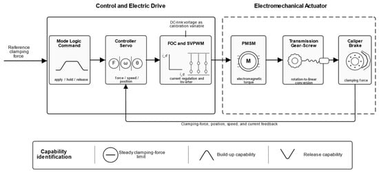
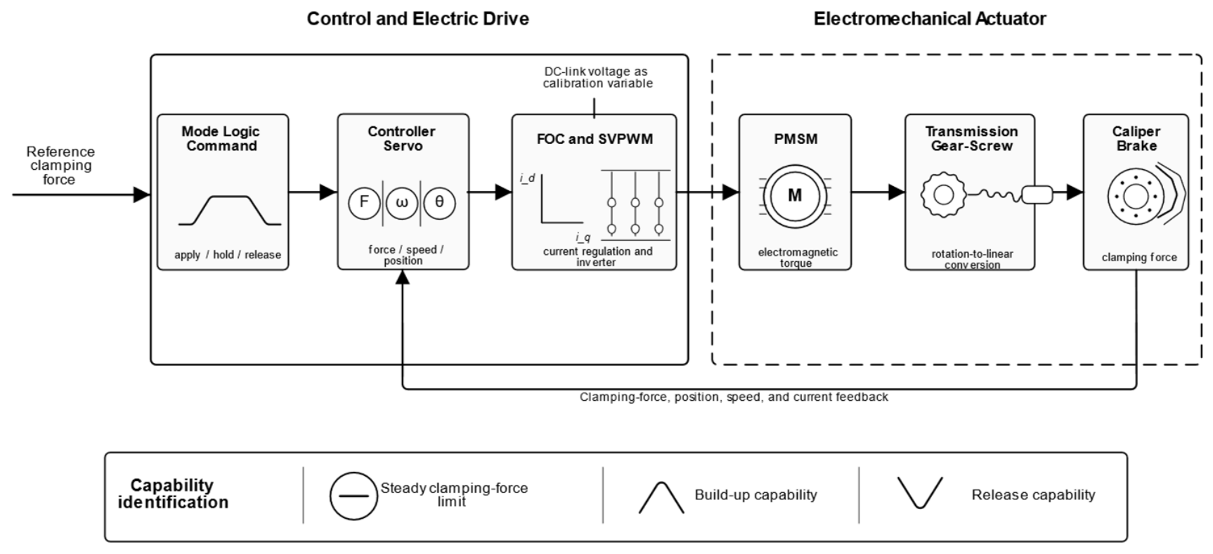
Under normal supply and identical wheel conditions, the lower-level actuators can generally track the nominal upper-level brake torque commands. When the bus voltage decreases, wheel supply states become unequal, or local actuator capability degrades; however, both the maximum output and the transient response rate become wheel-dependent. Commands based on an ideal actuator assumption may then exceed the available capability, increase tracking error, and create a transient left–right torque imbalance [24,25,26]. As shown in Figure 1, a single-wheel EMB is therefore used for capability calibration. The framework comprises the control and electric drive subsystem and the electromechanical actuator subsystem. DC bus voltage is the calibration variable, and the steady-state clamping force limit and the force application and release rates are the identified outputs.

Figure 1. Single-wheel EMB actuator capability calibration framework.

2.2. Single-Wheel EMB Actuator Model and Signal Flow

The single-wheel calibration model comprises a DC bus, a three-phase two-level inverter, field-oriented control (FOC) with space vector pulse-width modulation (SVPWM), a permanent-magnet synchronous motor (PMSM), reduction gearing, a ball screw, and a caliper load. Inputs are target clamping force and DC bus voltage; outputs include clamping force, screw displacement, motor speed, and d- and q-axis currents. Bus voltage is varied while the physical and controller parameters in Table 1 remain fixed.

Table 1. Main parameters of the single-wheel EMB calibration model.

Parameter	Value
Stator resistance	0.57 Ω
d- and q-axis inductance	8.5 mH
Permanent-magnet flux linkage	0.0155 Wb
Number of pole pairs	4
Rotor moment of inertia	3.42 × 10−5 kg·m2
Viscous damping coefficient	2.024 × 10−4 N·m·s·rad−1
SVPWM switching frequency	2 kHz
Reduction ratio	26.1
Ball-screw lead	5 mm/rev
Reduction mechanism efficiency	0.9
Ball-screw efficiency	0.9
Initial brake clearance	0.2 mm
d-axis current PI gains (Kp, Ki)	1, 1
q-axis current PI gains (Kp, Ki)	20, 1 × 10−4
Clamping force PID gains (Kp, Ki, Kd)	4, 1 × 10−5, 0.001
Clamping-force-to-brake torque coefficient KFT	0.1896 N·m/N

2.2.1. PMSM and Drive Control Model

In the synchronous rotating reference frame, the PMSM voltage equations can be written as:

$$u_d=R_s{i}_d+L_d{\displaystyle \frac{d{i}_d}{dt}}-{\omega }_e{L}_q{i}_q$$

(1)

$$u_q=R_s{i}_q+L_q{\displaystyle \frac{d{i}_q}{dt}}+{\omega }_e(L_d{i}_d+{\psi }_f)$$

(2)

The electromagnetic torque is:

$$T_e=\left({\displaystyle \frac{3}{2}}\right)p\left[{\psi }_f{i}_q+\left(L_d-L_q\right)i_d{i}_q\right]$$

(3)

The calibration model uses zero d-axis current control. Proportional–integral (PI) current controllers generate voltage commands, which are transformed using the inverse Park transformation and applied through SVPWM. Reduced bus voltage contracts the available voltage vector space and constrains current/torque build-up. Related studies address predictive current regulation [27], force-sensor fault tolerance [28], multi-loop clamping force control [29], contact point handling [30], nonlinear compensation [31], and variable universe fuzzy proportional–integral–derivative (PID) control [32].

2.2.2. Mechanical Transmission and Clamping Force Model

The motor angle is converted into axial displacement through the reduction mechanism and ball screw:

$$s={\displaystyle \frac{l_s{\theta }_m}{2\pi i_g}},x=s-x_0$$

(4)

where s is the axial displacement of the ball screw and x is the effective compression displacement after the initial clearance is eliminated. A piecewise nonlinear function is used to describe the relationship between clamping force and displacement, and the clamping force is converted into the equivalent motor shaft load torque as follows:

$$F_n(x)=\left\{\begin{array}{c}356.767x,x\le 0.112\\ -1805x^3+\mathrm{27,290}{x}^2-6036x+376.2,x>0.112\end{array}\right.$$

(5)

$$T_L={\displaystyle \frac{F_n{l}_s}{2\pi {\eta }_s{\eta }_g{i}_g}}$$

(6)

Capability calibration is performed in the clamping force domain and converted to wheel brake torque using Tb = KFT Fn, with KFT = 0.1896 N·m/N. The same conversion coefficient is used for calibration and the full-vehicle interface. Table 1 lists the actuator and controller parameters used in this study.

Equation (5) uses a published piecewise empirical clamping-force–displacement relation, also reported by Zou et al. ([33], Equation (24)), rather than a new fit identified in this study. The original point-level fitting dataset and its fit error statistics are not available in the present record; a new sample count or fitting accuracy is therefore not attributed to this relation. The actuator’s physical parameters were supplied for the study from product-related technical information; product-identifying details are confidential. These parameter inputs and the numerical controller settings in Table 1 do not constitute an independent experimental validation of the actuator model.

2.3. Influence of Low-Voltage Supply Constraints on Wheel-End Output Capability

The DC bus voltage determines the voltage space available to the inverter, which can be summarized by the following constraint:

$$u_d^2+u_q^2\le u_{\mathrm{m}\mathrm{a}\mathrm{x}}^2\left(U_{dc}\right)$$

(7)

When $U_{dc}$ decreases, the available voltage margin is reduced. During rapid clamping force build-up, reverse release, or periods of high motor back electromotive force, current regulation and electromagnetic torque response become more strongly constrained. After transmission through the mechanical drivetrain and caliper load, this effect appears as supply-dependent changes in the maximum steady-state clamping force, maximum rising rate, and maximum falling rate.

The steady-state clamping force limit is not assumed to be a linear function of bus voltage. Instead, it is treated as an effective capability boundary identified from the specified actuator model, controller parameters, and calibration command. For a given supply voltage, the single-wheel capability parameters are expressed as:

$F_{n,\mathrm{m}\mathrm{a}\mathrm{x}}\left(U_{dc}\right), {\dot{F}}_{n,\mathrm{u}\mathrm{p}}^{\mathrm{m}\mathrm{a}\mathrm{x}}\left(U_{dc}\right), {\dot{F}}_{n,\mathrm{d}\mathrm{o}\mathrm{w}\mathrm{n}}^{\mathrm{m}\mathrm{a}\mathrm{x}}\left(U_{dc}\right).$ The first term describes the steady-state magnitude capability, whereas the latter two terms describe the dynamic capability in the brake application and release directions, respectively. These three voltage-dependent mappings provide the single-wheel actuator capability boundaries. In Section 3, each wheel’s capability coefficient, the actual output of its previous cycle, and control period are further incorporated to form an online dynamic reachable interval.

2.4. Calibration of Wheel-End Capability Boundaries at Different Supply Voltages

2.4.1. Calibration Conditions and Data Processing

Clamp–hold–release simulations are performed at DC bus voltages of 12, 24, 36, and 48 V. The target clamping force steps from 0 to 50 kN at 0.5 s and is released to 0 at 3.0 s. The 18 and 30 V cases are not used for boundary fitting and are reserved for validating the piecewise linear interpolation.

The four equally spaced nodes cover a controlled sweep from severe undervoltage to the nominal 48 V supply; they are not claimed as standardized fault thresholds. The 50 kN input is a single-actuator calibration excitation, not a wheel-force demand derived from vehicle mass or target deceleration. With the adopted KFT, it corresponds to 9480 N·m at one wheel. Its purpose is to expose supply-dependent response under a common high command; vehicle braking demand is generated separately from pedal input in Section 3.1. Table 2 summarizes the excitation and processing settings.

Table 2. Capability boundary calibration and data-processing settings.

Parameter	Symbol	Setting
Main calibration bus voltage	Udc	12, 24, 36, 48 V
Interpolation-validation voltage	Uval	18, 30 V
Target clamping force	Fnref	50 kN
Brake application command time	tapply	0.5 s
Release command time	trelease	3.0 s
Fixed simulation step	Ts	5 × 10−5 s
Moving-average window	TMA	0.5 ms
Local fitting window	Tfit	5 ms

The steady-state clamping force is taken as the mean value over 2.8–3.0 s. To suppress SVPWM switching ripple, the raw clamping force is first processed using a 0.5 ms moving average. The local slope is then calculated by least-squares line fitting within a 5 ms sliding window. A 10 ms window is used only for sensitivity analysis and is not used for the main results.

2.4.2. Capability Boundary Extraction and Calibration Results

For a given bus voltage $U_{dc}$, the maximum steady-state clamping force is defined as the steady-state mean during the holding phase. The application rate limit is defined as the maximum positive local fitted slope during brake application, whereas the release rate limit is defined as the magnitude of the most negative local fitted slope during release:

$$F_{n,\mathrm{m}\mathrm{a}\mathrm{x}}\left(U_{dc}\right)=\mathrm{m}\mathrm{e}\mathrm{a}\mathrm{n}\left[{\bar{F}}_n\left(t\right)\right], t\in \left[2.8,3.0\right]\hspace{0.17em}\mathrm{s};$$

(8)

$${\dot{F}}_{n,\mathrm{u}\mathrm{p}}^{\mathrm{m}\mathrm{a}\mathrm{x}}\left(U_{dc}\right)=\mathrm{m}\mathrm{a}\mathrm{x}{\mathrm{S}\mathrm{l}\mathrm{o}\mathrm{p}\mathrm{e}}_{5\hspace{0.17em}\mathrm{m}\mathrm{s}}\left[{\bar{F}}_n\left(t\right)\right];$$

(9)

$${\dot{F}}_{n,\mathrm{d}\mathrm{o}\mathrm{w}\mathrm{n}}^{\mathrm{m}\mathrm{a}\mathrm{x}}\left(U_{dc}\right)=\mathrm{m}\mathrm{a}\mathrm{x}\left\{-{\mathrm{S}\mathrm{l}\mathrm{o}\mathrm{p}\mathrm{e}}_{5\hspace{0.17em}\mathrm{m}\mathrm{s}}\left[{\bar{F}}_n\left(t\right)\right]\right\}.$$

(10)

All three capability indices increase monotonically with bus voltage. The release rate limit is approximately 3.6–3.7 times the corresponding application rate limit, reflecting the asymmetric dynamics associated with elastic release and return control. Repeating the calculation with a 10 ms local fitting window changes each index by less than 1%, indicating that the identified rate boundaries are insensitive to the selected fitting-window length.

2.4.3. Capability Mapping and Interpolation Validation

Piecewise linear interpolation provides continuous capability estimates from the discrete calibration nodes in Table 3. It preserves the ordering of the tabulated values without introducing the curvature of an insufficiently identified nonlinear fit. The 18 and 30 V cases are withheld midpoints of the 12–24 V and 24–36 V intervals. Their relative errors in steady-state force, rising rate, and falling rate are 0.45%, 1.57%, and 2.10% at 18 V and 1.98%, 0.44%, and 2.82% at 30 V. These checks support interpolation at the tested interior points; they do not establish a uniform error bound, especially near 12 V. Further lower-bound and denser voltage checks are needed before extending this calibration claim.

Table 3. Identified EMB capability boundaries at different DC bus voltages.

Udc (V)	Fn,max (kN)	Rising Rate (kN/s)	Falling Rate (kN/s)
12	11.39	51.12	182.79
24	24.20	137.33	489.03
36	36.72	230.08	837.74
48	49.44	325.38	1213.85

Because the 48 V response approaches the 50 kN command, Table 3 provides effective boundaries for the specified excitation and controller, not absolute actuator maxima. The maps apply to the 12–48 V calibration range and fixed mechanical/controller conditions. Temperature, friction, wear, and other supply states require additional scheduling variables or updated capability estimates. The implementation includes below-12 V handling, but the present cases do not validate that branch or justify extrapolating these maps below their calibration range.

3. Four-Wheel EMB Brake Torque Allocation Based on Wheel-End Dynamic Reachable Sets

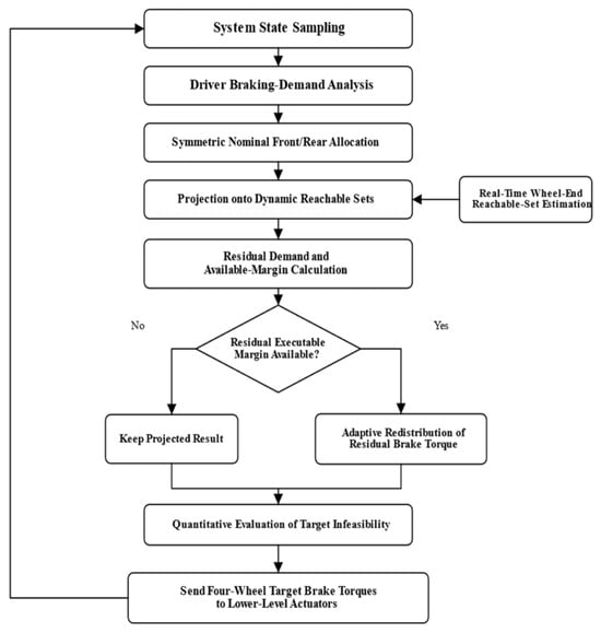
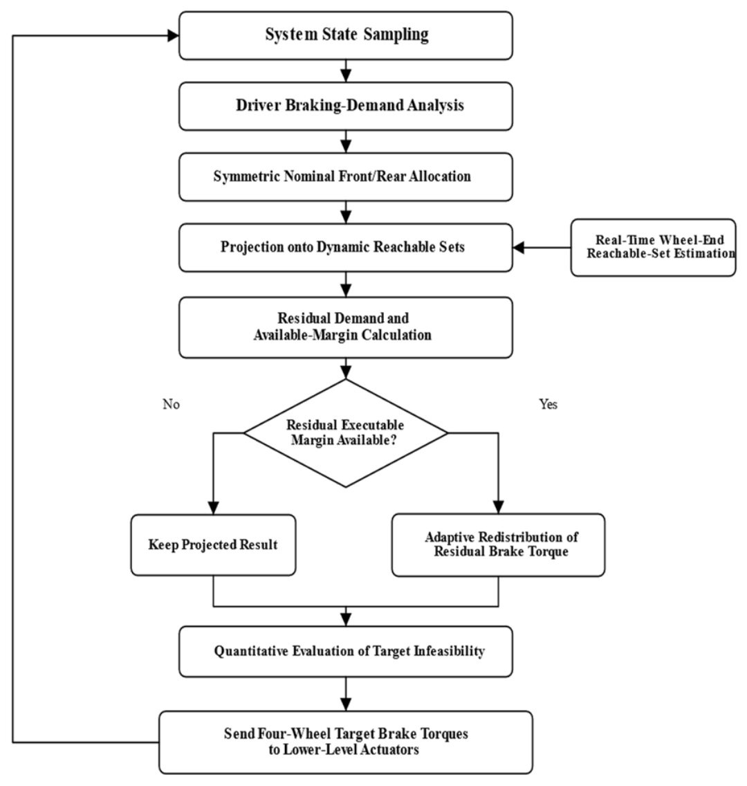
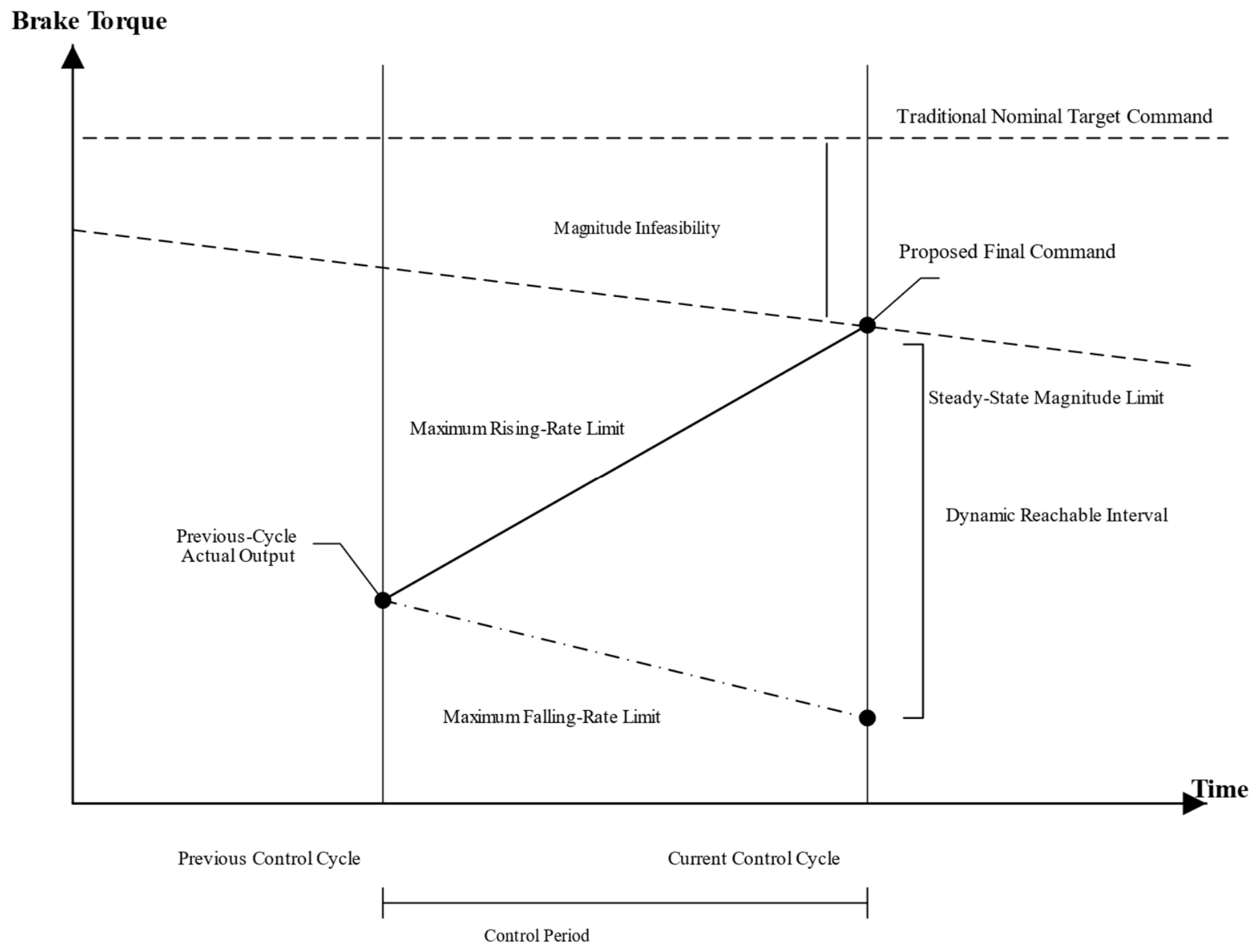
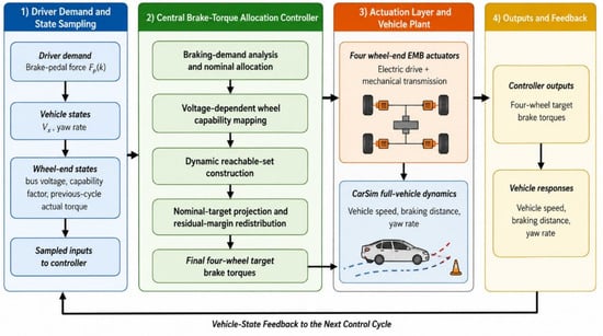
The controller extends the single-wheel capability maps to four wheel-specific dynamic intervals and then projects nominal targets and redistributes residual demand. Figure 2 summarizes this allocation procedure.

Figure 2. Four-wheel EMB brake torque allocation procedure.

3.1. Nominal Brake Torque Allocation

The proposed method retains the original vehicle-level braking-demand calculation and modifies only the wheel-level allocation to account for current actuation capability. To isolate the effect of the dynamic reachable-set constraint, a fixed front-rear axle ratio is adopted for the nominal allocation. The front-axle share is β = 0.60, and the rear-axle share is 0.40 in all cases. This fixed front-biased setting is used to isolate actuator-capability correction, not claimed as an optimum overload transfer or adhesion. Larger β loads the front-wheel intervals earlier; smaller β shifts the demand and residual margins rearward. Adaptive axle allocation can be coupled to the same wheel-end constraints.

The central controller obtains the total target vehicle brake torque from the driver brake-pedal input:

$$T_b^{\mathrm{d}\mathrm{e}\mathrm{m}}\left(k\right)=K_p\mathrm{m}\mathrm{a}\mathrm{x}\left[F_p\left(k\right)-F_{p,0},\hspace{0.17em}0\right]$$

(11)

where $F_p\left(k\right)$ is the brake-pedal input in the kth control cycle, $F_{p,0}$ is the pedal dead zone, $K_p$ is the braking-demand conversion coefficient, and $T_b^{\mathrm{d}\mathrm{e}\mathrm{m}}\left(k\right)$ is the total target vehicle brake torque.

Let the nominal front-axle brake torque allocation coefficient be $\beta$. The front- and rear-axle target brake torques are then expressed as:

$$T_{b,f}^{\mathrm{n}\mathrm{o}\mathrm{m}}\left(k\right)=\beta T_b^{\mathrm{d}\mathrm{e}\mathrm{m}}\left(k\right)$$

(12)

$$T_{b,r}^{\mathrm{n}\mathrm{o}\mathrm{m}}\left(k\right)=\left(1-\beta \right)T_b^{\mathrm{d}\mathrm{e}\mathrm{m}}\left(k\right)$$

(13)

For the straight-line braking cases considered in this study, the front- and rear-axle target torques are distributed symmetrically between the left and right wheels, yielding:

$$T_{b,\mathrm{F}\mathrm{L}}^{\mathrm{n}\mathrm{o}\mathrm{m}}\left(k\right)=T_{b,\mathrm{F}\mathrm{R}}^{\mathrm{n}\mathrm{o}\mathrm{m}}\left(k\right)={\displaystyle \frac{\beta T_b^{\mathrm{d}\mathrm{e}\mathrm{m}}\left(k\right)}{2}}$$

(14)

$$T_{b,\mathrm{R}\mathrm{L}}^{\mathrm{n}\mathrm{o}\mathrm{m}}\left(k\right)=T_{b,\mathrm{R}\mathrm{R}}^{\mathrm{n}\mathrm{o}\mathrm{m}}\left(k\right)={\displaystyle \frac{\left(1-\beta \right)T_b^{\mathrm{d}\mathrm{e}\mathrm{m}}\left(k\right)}{2}}$$

(15)

Let the wheel-end index set be $\mathcal{I}=\{\mathrm{F}\mathrm{L},\mathrm{F}\mathrm{R},\mathrm{R}\mathrm{L},\mathrm{R}\mathrm{R}\}$. The nominal target brake torques of the four wheels can then be written uniformly as $T_{b,i}^{\mathrm{n}\mathrm{o}\mathrm{m}}\left(k\right)$, $i\in \mathcal{I}$. These nominal allocation results satisfy the total vehicle braking demand but do not account for each wheel’s current supply state or actual actuation capability. Their feasibility therefore needs to be further constrained by the dynamic reachable set.

3.2. Construction of the Wheel-End Dynamic Reachable Set

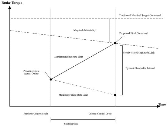
The wheel-end dynamic reachable set is jointly determined by the steady-state magnitude boundary and the rate boundaries over adjacent control cycles. According to the calibration results in Section 2, the mappings from bus voltage to the maximum achievable brake torque, maximum rising rate, and maximum falling rate are written as:

$$T_b^{\mathrm{m}\mathrm{a}\mathrm{x}}=f_T\left(U_{\mathrm{d}\mathrm{c}}\right)$$

(16)

$$r_{T,\mathrm{u}\mathrm{p}}^{\mathrm{m}\mathrm{a}\mathrm{x}}=f_{\mathrm{u}\mathrm{p}}\left(U_{\mathrm{d}\mathrm{c}}\right)$$

(17)

$$r_{T,\mathrm{d}\mathrm{o}\mathrm{w}\mathrm{n}}^{\mathrm{m}\mathrm{a}\mathrm{x}}=f_{\mathrm{d}\mathrm{o}\mathrm{w}\mathrm{n}}\left(U_{\mathrm{d}\mathrm{c}}\right)$$

(18)

For wheel $i$ in control cycle $k$, the measured bus voltage $U_{\mathrm{d}\mathrm{c},i}\left(k\right)$ yields the nominal capability boundaries under the current supply state:

$${\overline{T}}_{b,i}\left(k\right)=f_T\left[U_{\mathrm{d}\mathrm{c},i}\left(k\right)\right]$$

(19)

$${\overline{r}}_{b,i,\mathrm{u}\mathrm{p}}\left(k\right)=f_{\mathrm{u}\mathrm{p}}\left[U_{\mathrm{d}\mathrm{c},i}\left(k\right)\right]$$

(20)

$${\overline{r}}_{b,i,\mathrm{d}\mathrm{o}\mathrm{w}\mathrm{n}}\left(k\right)=f_{\mathrm{d}\mathrm{o}\mathrm{w}\mathrm{n}}\left[U_{\mathrm{d}\mathrm{c},i}\left(k\right)\right]$$

(21)

where ${\overline{T}}_{b,i}\left(k\right)$ is the maximum achievable brake torque, and ${\overline{r}}_{b,i,\mathrm{u}\mathrm{p}}\left(k\right)$ and ${\overline{r}}_{b,i,\mathrm{d}\mathrm{o}\mathrm{w}\mathrm{n}}\left(k\right)$ are the maximum brake torque rising and falling rates, respectively. To describe local degradation of wheel-end actuator capability, a capability coefficient ${\eta }_i\left(k\right)$ is introduced and constrained by 0 < ${\eta }_i\left(k\right)$ ≤ 1. It is set to 1 in the healthy state and to a value below 1 under degradation [20]. This study assumes a global proportional degradation of actuator performance and therefore uses a single capability coefficient. More complex non-proportional fault modes require a refined degradation model and are outside the present scope. The capability-adjusted boundaries are as follows: specifically, the same coefficient scales the maximum torque and both rate limits; ηRL = 0.3 therefore retains 30% of each healthy voltage-dependent boundary. This is a controlled proportional-derating case, not a fault-specific physical law or a standard-defined threshold. Non-proportional faults can instead use separate magnitude, application rate coefficients, and release rate coefficients without changing Equations (25)–(27).

$$T_{b,i}^{\mathrm{c}\mathrm{a}\mathrm{p}}\left(k\right)={\eta }_i\left(k\right){\overline{T}}_{b,i}\left(k\right)$$

(22)

$$r_{b,i,\mathrm{u}\mathrm{p}}\left(k\right)={\eta }_i\left(k\right){\overline{r}}_{b,i,\mathrm{u}\mathrm{p}}\left(k\right)$$

(23)

$$r_{b,i,\mathrm{d}\mathrm{o}\mathrm{w}\mathrm{n}}\left(k\right)={\eta }_i\left(k\right){\overline{r}}_{b,i,\mathrm{d}\mathrm{o}\mathrm{w}\mathrm{n}}\left(k\right)$$

(24)

The dynamic restriction as the actuator moves from its previous actual output toward the current target must also be considered. Let the actual brake torque in the previous control cycle be $T_{b,i}\left(k-1\right)$ and the control period be $T_s$. The dynamic upper and lower boundaries in the current cycle are then:

$$T_{b,i}^U\left(k\right)=\mathrm{m}\mathrm{i}\mathrm{n}\left[T_{b,i}^{\mathrm{c}\mathrm{a}\mathrm{p}}\left(k\right),\hspace{0.17em}{T}_{b,i}\left(k-1\right)+r_{b,i,\mathrm{u}\mathrm{p}}\left(k\right)T_s\right]$$

(25)

$$T_{b,i}^L\left(k\right)=\mathrm{m}\mathrm{a}\mathrm{x}\left[0,\hspace{0.17em}{T}_{b,i}\left(k-1\right)-r_{b,i,\mathrm{d}\mathrm{o}\mathrm{w}\mathrm{n}}\left(k\right)T_s\right]$$

(26)

At the first allocation update, the previous-output memory is initialized from the actuator’s initial actual torque; it is zero for the initially released brakes in the reported cases. Subsequent updates use the previous sampled actual torque, not the previous command. For a nonzero initial brake preload, that initial measured or estimated output must be used instead.

Accordingly, the dynamic reachable set of wheel $i$ in control cycle $k$ is defined as:

$${\Omega }_i\left(k\right)=\left[T_{b,i}^L\left(k\right),\hspace{0.17em}{T}_{b,i}^U\left(k\right)\right]$$

(27)

The interval is the one-step reachable output set of the stated magnitude/rate-bounded model. It is an engineering approximation to the full actuator dynamics. Its position and width depend on the previous actual output, supply voltage, capability coefficient, and control period, as illustrated in Figure 3.

Figure 3. Relationship between the dynamic boundary and the nominal target command.

3.3. Target Brake Torque Correction and Evaluation

The nominal target brake torque $T_{b,i}^{\mathrm{n}\mathrm{o}\mathrm{m}}\left(k\right)$ does not explicitly account for the current capability of each wheel. To ensure that the issued command lies within the achievable range, the nominal target is first projected onto the corresponding dynamic reachable set:

$$T_{b,i}^P\left(k\right)={\Pi }_{{\Omega }_i\left(k\right)}\left[T_{b,i}^{\mathrm{n}\mathrm{o}\mathrm{m}}\left(k\right)\right]$$

(28)

The projection operator can be expanded as:

$$T_{b,i}^P\left(k\right)=\mathrm{m}\mathrm{i}\mathrm{n}\left\{T_{b,i}^U\left(k\right),\hspace{0.17em}\mathrm{m}\mathrm{a}\mathrm{x}\left[T_{b,i}^L\left(k\right),\hspace{0.17em}{T}_{b,i}^{\mathrm{n}\mathrm{o}\mathrm{m}}\left(k\right)\right]\right\}$$

(29)

When the nominal target lies inside the dynamic reachable set, the projected result remains unchanged. When the nominal target exceeds the dynamic upper or lower boundary, the projection is set to the corresponding boundary. The total projected target torque carried by the four wheels is:

$$T_b^P\left(k\right)=\sum _{i\in \mathcal{I}}{T}_{b,i}^P\left(k\right)$$

(30)

The difference between the total vehicle braking demand and the projected total target torque is defined as:

$$\Delta T_b\left(k\right)=T_b^{\mathrm{d}\mathrm{e}\mathrm{m}}\left(k\right)-T_b^P\left(k\right)$$

(31)

When $\Delta T_b\left(k\right)$ is greater than 0, some wheels are limited by their capability boundaries and the projected total brake torque is below the driver demand; when $\Delta T_b\left(k\right)$ is less than 0, some wheels are constrained by the falling-rate limit during brake release and cannot yet decrease to the nominal target in the current cycle.

For the case in which $\Delta T_b\left(k\right)$ is greater than 0, the residual rising margin of each wheel below its dynamic upper boundary is first calculated:

$$H_{i,\mathrm{u}\mathrm{p}}\left(k\right)=T_{b,i}^U\left(k\right)-T_{b,i}^P\left(k\right)$$

(32)

The total residual rising margin of the four wheels is:

$$H_{\Sigma ,\mathrm{u}\mathrm{p}}\left(k\right)=\sum _{i\in \mathcal{I}}{H}_{i,\mathrm{u}\mathrm{p}}\left(k\right)$$

(33)

The brake torque that can actually participate in compensation is:

$$\Delta T_{b,\mathrm{u}\mathrm{p}}\left(k\right)=\mathrm{m}\mathrm{i}\mathrm{n}\left[\Delta T_b\left(k\right),\hspace{0.17em}{H}_{\Sigma ,\mathrm{u}\mathrm{p}}\left(k\right)\right]$$

(34)

When $H_{\Sigma ,\mathrm{u}\mathrm{p}}\left(k\right)$ is greater than 0, the compensation is distributed in proportion to each wheel’s residual margin relative to the total margin:

$$\Delta T_{b,i,\mathrm{u}\mathrm{p}}\left(k\right)={\displaystyle \frac{H_{i,\mathrm{u}\mathrm{p}}\left(k\right)}{H_{\Sigma ,\mathrm{u}\mathrm{p}}\left(k\right)}}\Delta T_{b,\mathrm{u}\mathrm{p}}\left(k\right)$$

(35)

During brake release, when $\Delta T_b\left(k\right)$ is less than 0, the residual falling margin of each wheel is defined as:

$$H_{i,\mathrm{d}\mathrm{o}\mathrm{w}\mathrm{n}}\left(k\right)=T_{b,i}^P\left(k\right)-T_{b,i}^L\left(k\right)$$

(36)

$$H_{\Sigma ,\mathrm{d}\mathrm{o}\mathrm{w}\mathrm{n}}\left(k\right)=\sum _{i\in \mathcal{I}}{H}_{i,\mathrm{d}\mathrm{o}\mathrm{w}\mathrm{n}}\left(k\right)$$

(37)

When $\Delta T_b\left(k\right)<0$ and $H_{\Sigma ,\mathrm{d}\mathrm{o}\mathrm{w}\mathrm{n}}\left(k\right)>0$, the brake torque that must be reduced and its wheel-end allocation are:

$$\Delta T_{b,\mathrm{d}\mathrm{o}\mathrm{w}\mathrm{n}}\left(k\right)=\mathrm{m}\mathrm{i}\mathrm{n}\left[-\Delta T_b\left(k\right),H_{\Sigma ,\mathrm{d}\mathrm{o}\mathrm{w}\mathrm{n}}\left(k\right)\right]$$

(38)

$$\Delta T_{b,i,\mathrm{d}\mathrm{o}\mathrm{w}\mathrm{n}}\left(k\right)={\displaystyle \frac{H_{i,\mathrm{d}\mathrm{o}\mathrm{w}\mathrm{n}}\left(k\right)}{H_{\Sigma ,\mathrm{d}\mathrm{o}\mathrm{w}\mathrm{n}}\left(k\right)}}\Delta T_{b,\mathrm{d}\mathrm{o}\mathrm{w}\mathrm{n}}\left(k\right)$$

(39)

After projection and residual-margin redistribution, the final target brake torque of each wheel is:

$$T_{b,i}^{\mathrm{r}\mathrm{e}\mathrm{f}}\left(k\right)=T_{b,i}^P\left(k\right)+\Delta T_{b,i,\mathrm{u}\mathrm{p}}\left(k\right)-\Delta T_{b,i,\mathrm{d}\mathrm{o}\mathrm{w}\mathrm{n}}\left(k\right)$$

(40)

Because the compensation is always limited by the current dynamic margin, the final target brake torque satisfies:

$$T_{b,i}^{\mathrm{r}\mathrm{e}\mathrm{f}}\left(k\right)\in {\Omega }_i\left(k\right), i\in \mathcal{I}$$

(41)

If the remaining executable margin of the four wheels is still insufficient to compensate for the total vehicle braking demand, the unresolved brake torque demand in the current cycle is defined as:

$$T_b^{\mathrm{r}\mathrm{e}\mathrm{m}}\left(k\right)=\mathrm{m}\mathrm{a}\mathrm{x}\left\{0,T_b^{\mathrm{d}\mathrm{e}\mathrm{m}}\left(k\right)-\sum _{i\in \mathcal{I}}{T}_{b,i}^{\mathrm{r}\mathrm{e}\mathrm{f}}\left(k\right)\right\}$$

(42)

The unresolved demand is calculated and reported to the vehicle-level controller each cycle. It is not accumulated into a command integrator, preventing windup in this residual-demand channel; this property alone is not a proof of complete actuator or vehicle closed-loop stability.

To quantitatively evaluate the match between target commands generated by different allocation methods and actual wheel-end responses, let the evaluation interval contain $N$ samples. For wheel $i$, let the final target brake torque and actual brake torque be $T_{b,i}^{\mathrm{r}\mathrm{e}\mathrm{f}}\left(k\right)$ and $T_{b,i}^{\mathrm{a}\mathrm{c}\mathrm{t}}\left(k\right)$, respectively. The four-wheel mean absolute brake torque tracking error is defined as:

$$E_{\mathrm{M}\mathrm{A}\mathrm{E}}={\displaystyle \frac{1}{4N}}{\displaystyle \sum _{k=1}^N}\sum _{i\in \mathcal{I}}\left|T_{b,i}^{\mathrm{a}\mathrm{c}\mathrm{t}}\left(k\right)-T_{b,i}^{\mathrm{r}\mathrm{e}\mathrm{f}}\left(k\right)\right|$$

(43)

The metric is expressed in N·m, and a smaller value indicates closer tracking between the final target torque and the actual wheel-end output. For each comparison method, the target term is the final command sent to the wheel-end actuator by that method, ensuring a consistent comparison.

To evaluate the mismatch between a candidate target command and the wheel-end dynamic reachable set, let the candidate command of wheel $i$ be $T_{b,i}^c\left(k\right)$. Its instantaneous infeasible amount relative to the dynamic reachable set is defined as:

$$e_{\mathrm{i}\mathrm{n}\mathrm{f},i}\left(k\right)=\left|T_{b,i}^c\left(k\right)-{\Pi }_{{\Omega }_i\left(k\right)}\left[T_{b,i}^c\left(k\right)\right]\right|$$

(44)

When the candidate command lies inside ${\Omega }_i\left(k\right)$, $e_{\mathrm{i}\mathrm{n}\mathrm{f},i}\left(k\right)=0$; when it lies outside the dynamic reachable set, this index equals the distance between the candidate command and the nearest achievable boundary. Time-domain accumulation over the entire braking process gives the cumulative dynamic infeasibility:

$$J_{\mathrm{i}\mathrm{n}\mathrm{f}}=T_s{\displaystyle \sum _{k=1}^N}\sum _{i\in \mathcal{I}}{e}_{\mathrm{i}\mathrm{n}\mathrm{f},i}\left(k\right)$$

(45)

where $T_s$ is the brake torque allocation control period and $J_{\mathrm{i}\mathrm{n}\mathrm{f}}$ is expressed in N·m·s. A smaller value indicates a lower mismatch between the candidate target command and the instantaneous wheel-end dynamic capability. To distinguish target commands before and after dynamic-reachable-set correction, the following quantities are further defined:

$$J_{\mathrm{r}\mathrm{a}\mathrm{w}}=J_{\mathrm{i}\mathrm{n}\mathrm{f}}\left(T_{b,i}^{\mathrm{n}\mathrm{o}\mathrm{m}}\right)$$

(46)

$$J_{\mathrm{f}\mathrm{i}\mathrm{n}\mathrm{a}\mathrm{l}}=J_{\mathrm{i}\mathrm{n}\mathrm{f}}\left(T_{b,i}^{\mathrm{r}\mathrm{e}\mathrm{f}}\right)$$

(47)

where $J_{\mathrm{r}\mathrm{a}\mathrm{w}}$ reflects the mismatch between the nominal allocation command and the current wheel-end capability, whereas $J_{\mathrm{f}\mathrm{i}\mathrm{n}\mathrm{a}\mathrm{l}}$ reflects the dynamic feasibility of the final issued command. Because DRA uses projection to constrain the final target inside the dynamic reachable set, its $J_{\mathrm{f}\mathrm{i}\mathrm{n}\mathrm{a}\mathrm{l}}$ value being close to zero is a constraint-consistency result determined by the algorithmic structure. Therefore, the subsequent simulations evaluate performance jointly using $E_{\mathrm{M}\mathrm{A}\mathrm{E}}$ and the vehicle longitudinal and yaw responses.

3.4. Feasibility, Sensitivity, and Computational Properties

For nonempty intervals, projection places each wheel command inside its bounds. During demand increase, the compensation fraction is min(ΔT, ΣHi)/(ΣHi), which lies between zero and one whenever ΣHi > 0. Each increment is therefore no greater than its available margin Hi. The same argument applies to release margins. Equations (40) and (41) consequently preserve interval membership and bound the issued command by the modeled magnitude limit. Reapplying this argument gives per-cycle feasibility conditional on valid, nonempty intervals; it does not establish recursive feasibility through arbitrary abrupt capability loss. An incompatible lower/upper bound requires supervisory handling rather than an assumed feasible projection.

Endpoint sensitivity follows directly from Equations (25) and (26). With fixed active limits, a previous torque error shifts the corresponding rate endpoint by the same amount, and a rate error δr changes it by Ts δr. Changing the allocation period by δTs changes the rate contribution by r δTs. On a linear map segment, voltage error propagates through that segment’s slope; proportional capability error changes each boundary in proportion to its healthy mapped value. Min/max and projection operations are continuous and nonexpansive in their scalar inputs for fixed bounds. These observations identify error pathways, not a closed-loop robustness guarantee: optimistic capability estimates can permit unachievable commands, while underestimated capability sacrifices usable braking demand.

DRA uses a fixed sequence of map interpolation, min/max operations, projection, margin sums, and proportional redistribution. With a fixed-size calibration table, arithmetic work and storage scale as O(n) for n wheels; no iterative optimizer is invoked. The allocation period is 0.01 s (100 Hz). This operation-level comparison is distinct from measured CPU time: target-processor worst-case execution time and scheduling margin remain implementation-validation tasks. Appendix A gives the complete QP-D formulation and fixed numerical settings.

4. Results and Discussion

The four methods are compared using MATLAB/Simulink–CarSim co-simulation under normal supply, synchronized low voltage, unequal wheel voltages, and single-wheel degradation. Baseline retains fixed-ratio allocation; Static adds magnitude saturation; QP-D and DRA use the same capability map definitions, wheel supply/degradation inputs, 0.01 s allocation period, and previous-actual-torque convention. Their instantaneous intervals depend on their respective actual torque histories. QP-D additionally includes yaw and output-change penalties and a soft yaw constraint; the algorithms therefore do not have identical allocation objectives. Appendix A documents the fixed QP-D benchmark.

The evaluation interval starts at t = 1.0 s, when the pedal reaches 350 N, and ends at the first decrease in longitudinal speed to 0.5 km/h. Thus the 0.8–1.0 s pedal ramp is excluded from the reported duration and distance but included in the simulated histories. Reported quantities include braking duration/distance, actual total torque, integrated demand deficit, peak and root mean square (RMS) yaw rate, and additional braking yaw moment. The peak total torque uses the simultaneous sum of actual wheel outputs. Figure 9 reports offline nominal-command infeasibility and projection frequency; these are model consistency measures, not independent experimental validation. Each case is deterministic; numerical differences describe the stated runs and are not statistical confidence estimates.

4.1. Co-Simulation Platform and Test Cases

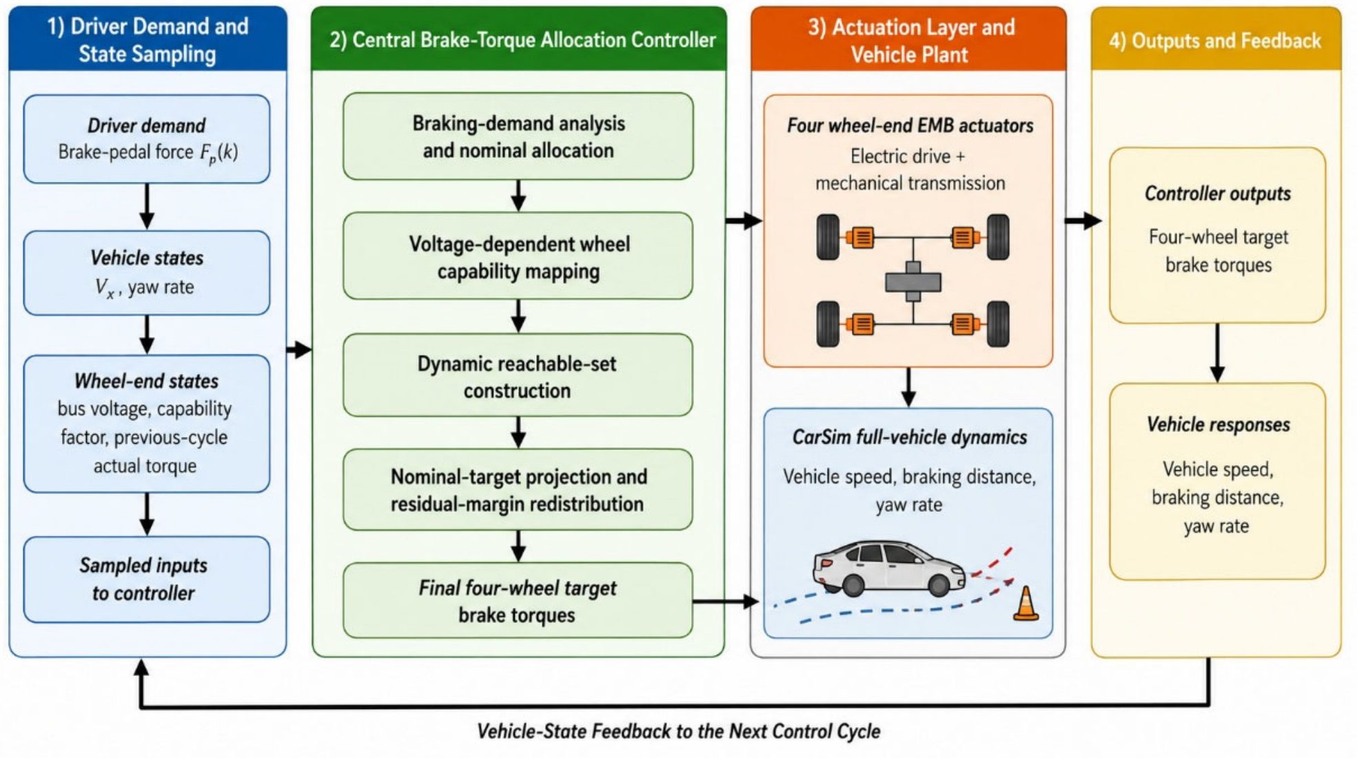
The co-simulation platform consists of an upper-level brake torque allocation controller, four EMB actuator models, and a CarSim full-vehicle dynamics model. The upper-level controller calculates the total vehicle braking demand from the driver input and updates the wheel-end dynamic reachable boundaries using each wheel’s bus voltage and capability coefficient. It then corrects the nominal brake torque commands and redistributes torque according to the residual dynamic margin of each wheel.

The wheel-end models describe the dynamic relationship between target brake torque, clamping force, and actual brake torque. CarSim receives the four actual wheel torques and calculates vehicle speed, travel distance, yaw rate, and other vehicle states. The resulting information flow is braking-demand generation, target-torque allocation, actuator response, and vehicle-dynamics feedback. Figure 4 shows the platform topology, while Table 4 and Table 5 list the simulation parameters and test cases, respectively. All four allocation methods use identical vehicle parameters, a 350 N brake input, simulation step size, and initial conditions; only the wheel-end bus voltages and capability coefficients vary among cases.

Figure 4. MATLAB/Simulink–CarSim co-simulation platform.

Table 4. Co-simulation platform settings.

Category	Parameter	Setting
Initial vehicle state	Initial longitudinal speed	80 km/h
Road condition	Road type	Flat, straight road
Road condition	Road friction coefficient	0.85; identical left/right adhesion
Driver input	Steering-wheel angle	0°
Driver input	Throttle opening	0
Brake input	Pedal-force profile	0–0.8 s: 0 N
Brake input	Pedal-force profile	0.8–1.0 s: increases from 0 to 350 N
Brake input	Pedal-force profile	1.0–6.0 s: held at 350 N
Brake input	Pedal-force profile	6.0–6.2 s: decreases to 0 N
Brake input	Pedal-force profile	6.2–8.0 s: held at 0 N
Simulation setting	Simulation time	8 s
Simulation setting	CarSim co-simulation step	0.0005 s
Controller setting	DRA control period	0.01 s

Table 5. Test-case settings.

Case	Condition	Setting
Comparison methods	Brake torque allocation	Baseline, Static, QP-D, DRA
Case 1	Normal supply	Wheel voltages [48, 48, 48, 48] V; all capability coefficients = 1
Case 2	Synchronized low voltage	Wheel voltages [24, 24, 24, 24] V; all capability coefficients = 1
Case 3	Unequal wheel voltages	[FL, FR, RL, RR] = [48, 36, 24, 12] V; all capability coefficients = 1
Case 4	Rear-left capability degradation	All wheel voltages = 48 V; RL capability coefficient = 0.3; the other three = 1

MATLAB/Simulink R2022b (The MathWorks, Inc., Natick, MA, USA) implements allocation and the four EMB models; CarSim 2019 (Mechanical Simulation Corporation, Ann Arbor, MI, USA) supplies the C-Class Hatchback vehicle model through the Simulink co-simulation interface. The CarSim configuration uses AB-2 integration with a 0.0005 s model step and a 0.025 s output-file interval. These settings are distinct from the 0.01 s allocation period and the 0.00005 s single-wheel calibration step in Table 2. Figure 4 identifies the exchanged physical signals: issued wheel torques drive the EMB models, actual actuator outputs enter the vehicle model, and vehicle states provide the response metrics. Table 4 separates the vehicle, input, and timing settings.

Table 5 varies one actuator-side factor at a time. Voltages and capability coefficients are held constant within each case to isolate the allocation response; the online equations accept time-varying sampled inputs, but abrupt sags and recovery require separate validation. The common friction coefficient of 0.85 isolates actuator capability on a straight, uniform-adhesion road. Low-adhesion and split-friction cases additionally require tire-force/slip constraints and coordinated stability control; conclusions here are limited to the stated road conditions.

4.2. Normal Four-Wheel Supply

Under normal four-wheel supply, all wheel bus voltages are set to 48 V and all capability coefficients are 1. This case is used to determine whether the dynamic reachable-set constraint introduces an additional loss of longitudinal braking performance when wheel-end capability is sufficient and left–right symmetric.

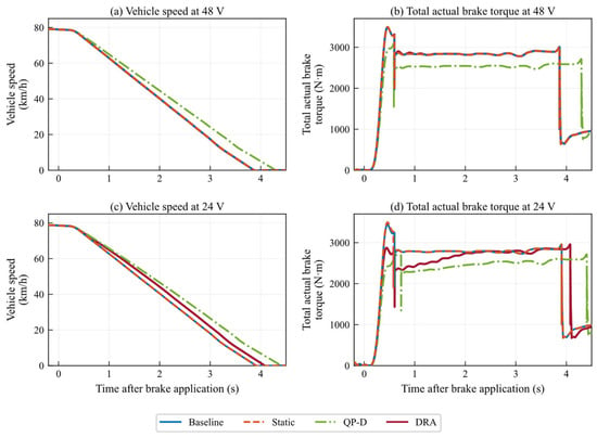
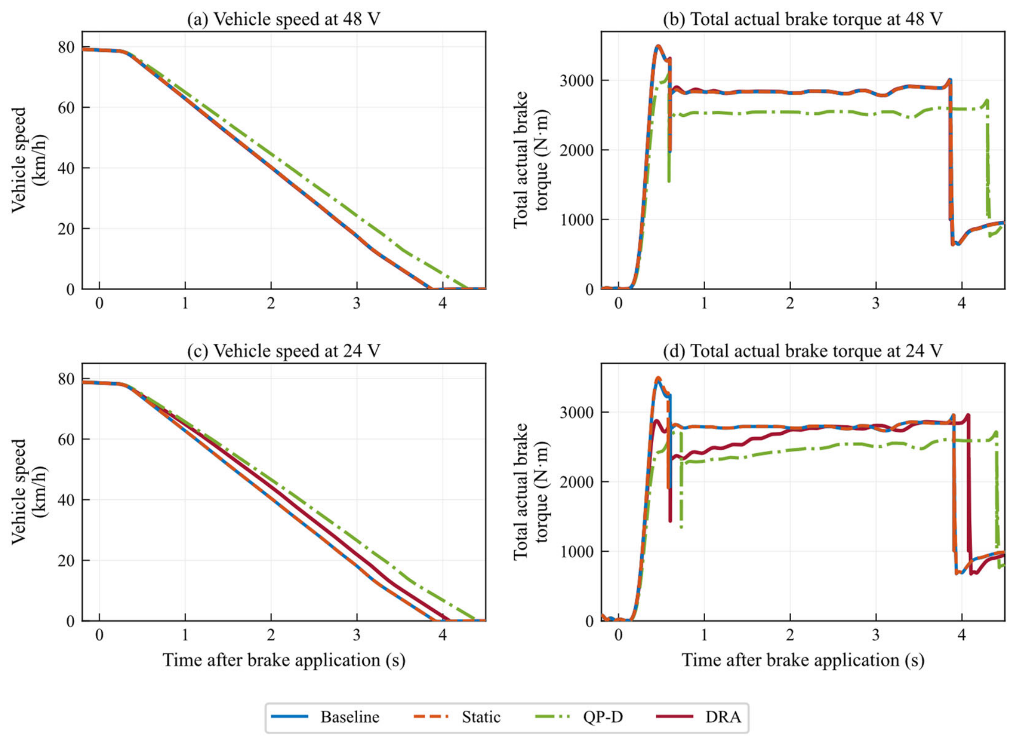
Figure 5a shows nearly overlapping speed responses for Baseline, Static, and DRA, whereas QP-D decelerates more slowly. The respective brake-onset speeds are 78.69, 78.69, 78.70, and 78.69 km/h. Durations and distances are collected in Table 6. DRA and Static differ by approximately 0.005 s and 0.08 m in this deterministic case; these small differences indicate limited intervention here, not a statistically established improvement or universal nominal transparency.

Figure 5. Longitudinal responses: (a,b) all wheels at 48 V; (c,d) all wheels at 24 V. All capability coefficients equal 1.

Table 6. Braking duration and distance from t = 1.0 s to the 0.5 km/h threshold.

Case	Method	Duration (s)	Distance (m)
48 V	Baseline	3.6440	40.3310
48 V	Static	3.6440	40.3310
48 V	QP-D	4.0700	45.1368
48 V	DRA	3.6390	40.2558
24 V	Baseline	3.6820	40.5037
24 V	Static	3.6820	40.5067
24 V	QP-D	4.1770	46.8876
24 V	DRA	3.8525	43.5829
Unequal voltages	Baseline	3.6275	39.9706
Unequal voltages	Static	3.4590	38.2231
Unequal voltages	QP-D	3.2465	37.4179
Unequal voltages	DRA	3.4475	38.2046
RL degradation	Baseline	3.6335	40.2456
RL degradation	Static	3.5770	39.6950
RL degradation	QP-D	4.2075	49.9272
RL degradation	DRA	3.6550	42.3916

Figure 5b shows that the peak total actual brake torques of Baseline, Static, and DRA are all 3491.9 N·m, whereas that of QP-D is 3096.9 N·m. The peak and RMS yaw rates are zero for all four methods, indicating that no additional directional response is generated when the left–right supply and capability states are symmetric.

QP-D travels approximately 12% farther than DRA in the nominal case, with integrated demand deficits of 3444.1 and 1974.4 N·m·s, respectively. This is a material benchmark difference, not an intrinsic consequence of quadratic programming. Its objective balances demand tracking against deviation from the previous actual output; during torque build-up these objectives can compete even with zero yaw. Appendix A discloses the normalization, all weights, constraints, and fallback. The aggregate results do not isolate the contributions of weighting, actuator lag, or fallback events, so they are not used to establish optimal tuning or exclude implementation-related effects. The comparison supports the stated fixed configuration rather than a ranking of all QP allocators.

The nominal case therefore assesses the intervention introduced by dynamic capability correction; it is not used as evidence of improved nominal braking effectiveness.

4.3. Synchronized Four-Wheel Low-Voltage Case

To analyze the influence of an overall reduction in supply voltage on brake torque allocation, all four wheel bus voltages are reduced to 24 V while the capability coefficients remain 1. Because the four-wheel supply state remains symmetric, this case mainly reflects how reduced wheel-end torque build-up capability under low voltage affects longitudinal vehicle response.

As shown in Figure 5c, the braking durations of Baseline, Static, QP-D, and DRA are 3.6820, 3.6820, 4.1770, and 3.8525 s, respectively, and the corresponding braking distances are 40.5037, 40.5067, 46.8876, and 43.5829 m. Relative to QP-D, DRA reduces braking duration by 7.77% and braking distance by 7.05%, indicating a smaller longitudinal-performance penalty while satisfying the low-voltage dynamic capability constraints.

In Figure 5d, the peak total actual brake torques of Baseline, Static, QP-D, and DRA are 3444.2, 3497.1, 2714.1, and 2913.5 N·m, respectively. Their integrated brake demand deficits are 2167.6, 2173.0, 3863.0, and 2749.5 N·m·s, respectively. The integrated deficit of DRA is 28.8% lower than that of QP-D, showing lower demand loss than the disclosed fixed QP-D configuration in this case.

Relative to Static, DRA increases braking distance by 7.59% and decreases peak actual total torque by 16.69%. This is a genuine longitudinal cost, not a safety benefit by itself. Static permits commands beyond the one-step rate boundary, whereas DRA modifies them before issue. The result demonstrates a trade-off between modeled command feasibility and stopping performance; acceptable vehicle-level operation also requires adequate deceleration and directional stability.

Because the four-wheel capabilities remain symmetric, the yaw rate is zero for all four methods. DRA enforces the transient capability constraints but incurs a moderate longitudinal-performance penalty relative to Static, which enforces only steady-state magnitude limits.

4.4. Unequal Four-Wheel Voltage Case

In the unequal-voltage case, the bus voltages of FL, FR, RL, and RR are set to 48, 36, 24, and 12 V, respectively. The steady-state output and dynamic-rate capabilities therefore differ substantially among wheels. This case is used to examine the relationship between longitudinal braking-demand satisfaction and left–right brake-force coordination under asymmetric capability.

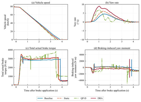
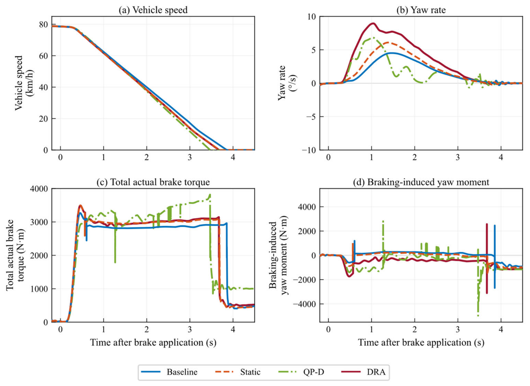
As shown in Figure 6a,c and Table 6, DRA and Static have nearly equal braking distances (38.2046 and 38.2231 m). Their integrated demand deficits are 1395.9 and 1413.6 N·m·s, respectively. QP-D gives both a shorter distance (37.4179 m) and a smaller deficit (887.1 N·m·s) than DRA in this case; Baseline gives 39.9706 m and 1976.7 N·m·s.

Figure 6. Vehicle responses with [FL, FR, RL, RR] voltages = [48, 36, 24, 12] V and all capability coefficients = 1.

Figure 6b shows peak yaw rates of 4.51, 6.10, 6.84, and 8.95°/s for Baseline, Static, QP-D, and DRA; the corresponding RMS values are 2.4710, 3.3278, 3.0645, and 5.1788°/s. DRA produces the largest peak and RMS yaw response. Its RMS is approximately 1.69 times that of QP-D, demonstrating a substantial directional-control limitation under the specified asymmetric capability.

Figure 6d shows that the peak additional braking yaw moment of DRA is 1738.7 N·m, lower than the 2810.3 N·m of QP-D. However, the absolute integral of the yaw moment for DRA is 1590.4 N·m·s, which is higher than the 1438.8 N·m·s of QP-D. This result indicates that the vehicle yaw response depends not only on the instantaneous peak but also on the duration and direction of the additional yaw moment. The command-level yaw proxy constrained in QP-D must be distinguished from the vehicle-response moment calculated from actual outputs; a soft constraint on the former is not a hard bound on the latter.

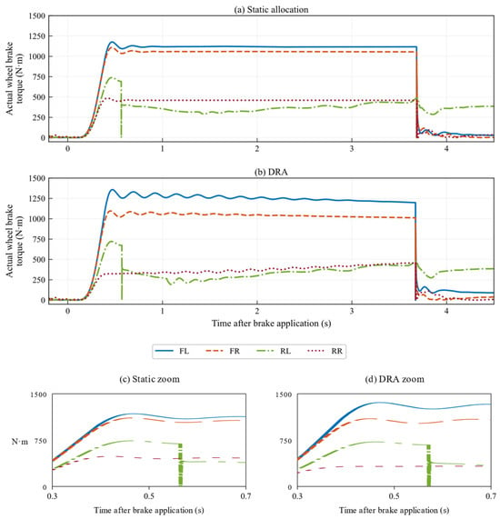
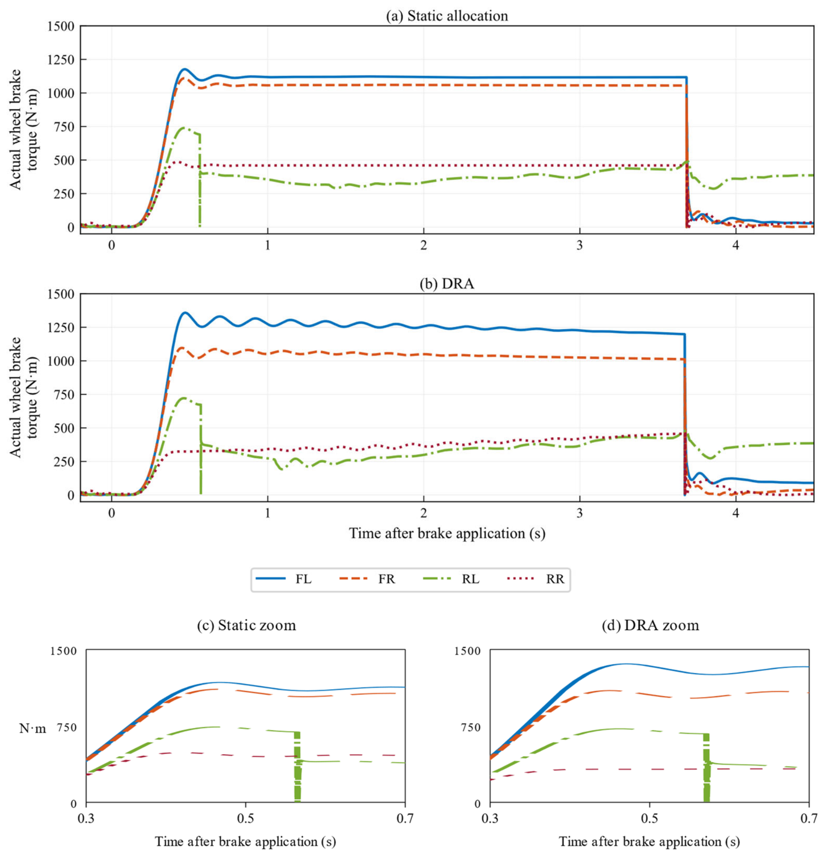
Figure 6 compares the methods in terms of vehicle speed, total actual brake torque, yaw rate, and additional braking yaw moment. To further examine the formation of wheel-end outputs, Figure 7 compares the four actual wheel brake torques of Static and DRA.

Figure 7. Actual wheel torques at [FL, FR, RL, RR] = [48, 36, 24, 12] V; all capability coefficients = 1. (a) Static; (b) DRA; (c,d) corresponding enlarged views around 0.5 s on the plotted time-after-brake-application axis. Enlargements use the original plotted curves, without new simulation data.

Figure 7 shows a strongly limited 12 V right-rear output and unequal compensating outputs at the other wheels. The DRA law allocates residual demand in proportion to scalar margins, without left–right pairing or yaw moment weighting. Greater available margin can therefore draw compensation toward one side. This mechanism is consistent with the persistent torque imbalance and larger absolute moment integral, even though DRA has a smaller moment peak than QP-D. The result also explains why peak moment alone does not predict the ordering of yaw-rate responses.

A yaw-aware extension can retain the same wheel-end bounds while selecting the redistribution increment subject to a constraint on the predicted command-level moment, |c^T(Tproj + ΔT) − Mz,ref| ≤ Mz,allow, together with the available increment margins. Alternatively, a moment-error penalty can be combined with demand recovery. The desired moment and allowable error must come from vehicle-level coordination, and conflicting demand/yaw constraints need explicit prioritization. This is an integration formulation, not an additional controller evaluated in the present results. The observed limitation concerns the current scalar redistribution law and does not remove the need for voltage-dependent wheel-end constraints.

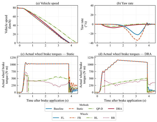
4.5. Rear-Left Actuator Capability-Degradation Case

Single-wheel EMB degradation creates a conflict between longitudinal braking-demand satisfaction and lateral stability because the left–right brake-force symmetry is broken [34]. To analyze allocation under single-wheel actuator degradation, all four wheel bus voltages are set to 48 V, while the capability coefficient of the rear-left (RL) wheel is reduced to 0.3 and those of the other three wheels remain at 1. This case is used to examine the differences among the allocation methods in longitudinal braking efficiency and yaw suppression when the degraded wheel is output-limited. The value 0.3 is a severe illustrative derating chosen to expose redistribution clearly, not a standard-mandated threshold. Under the stated proportional model, coefficients 1.0, 0.7, 0.5, and 0.3 retain 100%, 70%, 50%, and 30% of each healthy boundary, respectively. This algebraic scaling should not be interpreted as a vehicle-response sweep or as monotonic yaw improvement with coefficient changes.

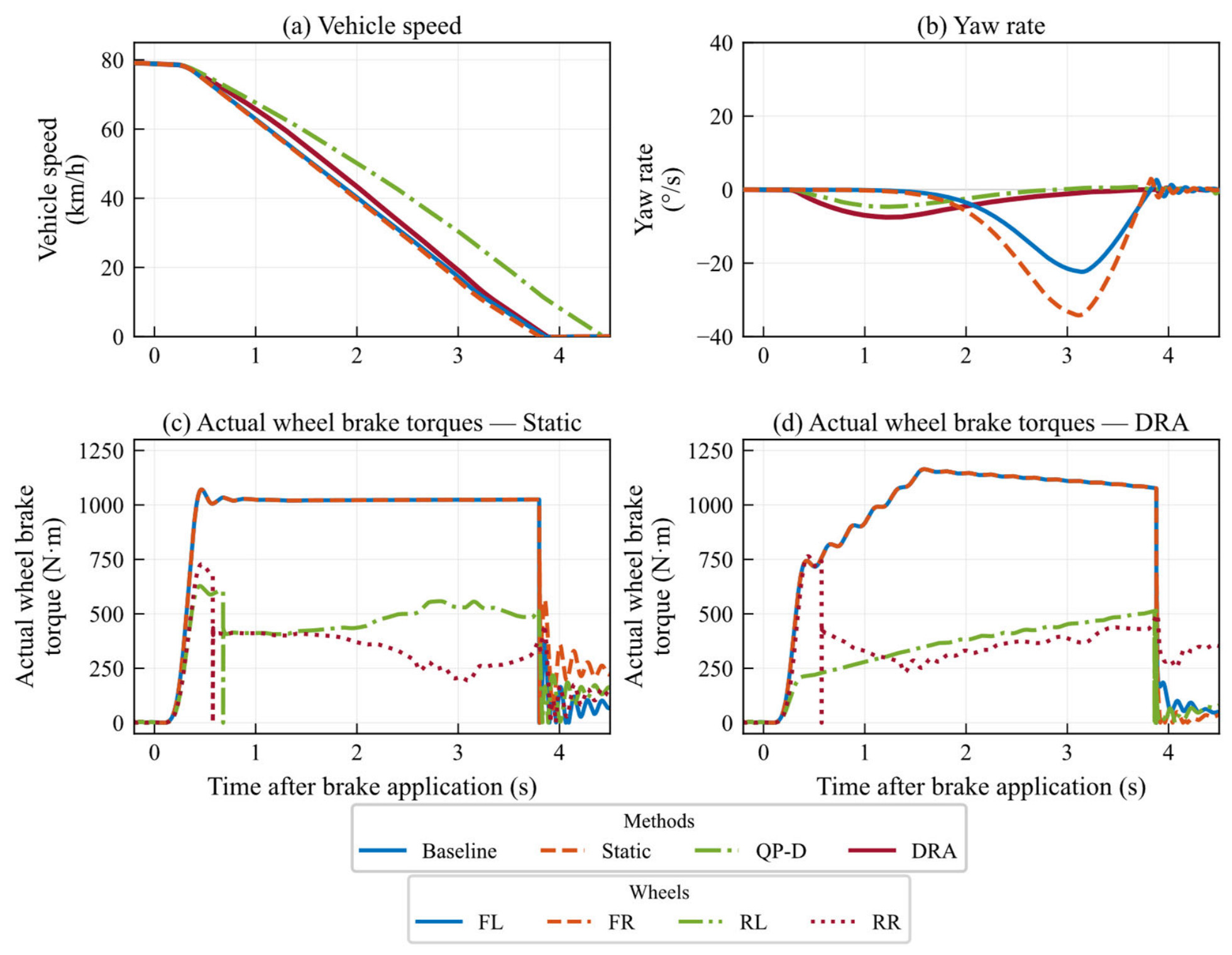
As shown in Figure 8a, the braking durations of Baseline, Static, QP-D, and DRA are 3.6335, 3.5770, 4.2075, and 3.6550 s, respectively, and the braking distances are 40.2456, 39.6950, 49.9272, and 42.3916 m. The corresponding integrated brake demand deficits are 2013.6, 1914.7, 3932.5, and 2045.8 N·m·s. Relative to Baseline and Static, DRA increases braking distance by 5.33% and 6.79%, respectively.

Figure 8. Vehicle and wheel-end responses with all wheels at 48 V, ηRL = 0.3, and the other capability coefficients = 1.

In Figure 8b, the peak yaw rates of Baseline, Static, QP-D, and DRA are 22.38, 34.20, 4.68, and 7.52°/s, respectively. Relative to Baseline and Static, DRA reduces peak yaw rate by 66.4% and 78.0%, and reduces RMS yaw rate by 59.1% and 73.5%, respectively. These results show that dynamic capability constraints and redistribution using the remaining capability of healthy wheels can substantially mitigate the directional response caused by single-wheel degradation.

Figure 8c,d show that Static mainly imposes a steady-state magnitude limit on the degraded wheel, whereas DRA reduces the command according to the wheel’s dynamic capability and redistributes the remaining demand among the healthy wheels. QP-D further decreases the peak yaw rate to 4.68°/s; however, relative to QP-D, DRA shortens the braking distance by 15.09% and reduces the integrated brake demand deficit by 47.98%.

In this degradation case, QP-D gives the smaller yaw response while DRA gives the shorter distance and lower demand deficit. These outcomes demonstrate different allocation priorities in the same modeled actuator environment rather than a single best method across all vehicle objectives.

4.6. Overall Evaluation of Vehicle Performance and Dynamic Feasibility

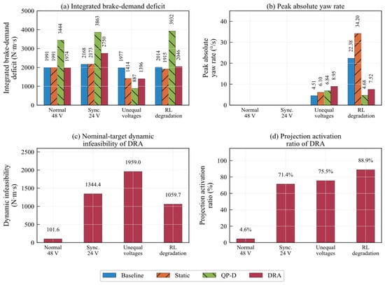
For an overall comparison, Figure 9a,b present the integrated brake demand deficit and peak yaw rate, respectively, while Figure 9c,d show the cumulative dynamic infeasibility of the DRA nominal targets and the projection-trigger ratio. These feasibility indices are reconstructed offline from the saved actual wheel torques, bus voltages, and capability coefficients using the same capability maps as the online controller. They therefore quantify whether the nominal targets lie within the corresponding one-step dynamic intervals.

Figure 9. Vehicle-performance and dynamic-feasibility metrics.

The offline reconstruction shows that the cumulative dynamic infeasibility of the DRA nominal targets is 101.6, 1344.4, 1959.0, and 1059.7 N·m·s under normal 48 V supply, synchronized 24 V supply, unequal wheel voltages, and rear-left degradation, respectively. The corresponding projection-trigger ratios are 4.6%, 71.4%, 75.5%, and 88.9%. Projection is rarely activated in the normal case, whereas the trigger ratio exceeds 70% in all three capability-limited cases, indicating that nominal allocation frequently falls outside the one-step dynamic reachable range.

Table 6 consolidates braking duration and distance over the common evaluation definition. The extra digits preserve the original simulation outputs for traceability; they do not imply equivalent experimental accuracy.

4.7. Functional Safety Considerations and Validation Limits

The common actuator model provides a controlled model-in-the-loop (MIL) comparison, but using it for both calibration and evaluation does not independently validate physical EMB behavior. The interpolation checks test held-out voltages within that model; zero final-command infeasibility tests allocation consistency. Independent current, speed, clamping force, and torque measurements are needed to assess model mismatch. A subsequent bench/HIL campaign should validate the actuator first and then examine voltage transients, temperature/wear, non-proportional faults, low/split adhesion, and combined steering/braking. Repeating an unchanged deterministic run would not characterize these uncertainties; meaningful variability estimates require defined perturbations or independent measurements.

In a functional safety architecture such as that addressed by ISO 26262 [35], DRA is an allocation layer, not a complete safety mechanism. Bus voltage, previous actual torque, and capability coefficients are available model signals in the reported cases. Production integration requires a diagnostic/estimation layer with range, plausibility, freshness, and fault-persistence checks. Capability coefficients would have to be obtained from validated health estimation, not inferred from the allocation equations alone. Overestimating capability can make the modeled interval optimistic; signal-validation faults therefore need supervisory intervention.

The implemented residual-demand output in Equation (42) provides a supervision interface. Emergency thresholds must depend on required deceleration, speed, yaw, demand-deficit duration, and the vehicle hazard analysis; no universal threshold or ASIL claim is assigned here. A safety supervisor must also detect incompatible intervals and multi-wheel loss of capability. DRA cannot recover braking torque that no wheel can deliver. A fail-operational or fail-safe response requires vehicle-specific redundancy, diagnostics, and a validated fallback, distinct from the numerical QP fallback in Appendix A. Below-12 V handling in the implementation is likewise not evidence of validated severe-undervoltage braking.

Strong asymmetry needs particular attention: the unequal-voltage result precludes treating current DRA redistribution as a standalone yaw-safety function. A yaw monitor and coordinated yaw/tire-force constraints are required for that application. Functional safety integration additionally requires hazard analysis, integrity allocation, diagnostic coverage, dependent-failure assessment, and execution-time verification. These system-level obligations are separated from the command-feasibility properties established in Section 3.4.

5. Conclusions

This study addresses the possibility that nominal four-wheel EMB brake torque commands may exceed transient actuator capability under low-voltage supply or unequal wheel-end capability. The proposed allocation method identifies voltage-dependent steady-state and torque-rate boundaries using a single-wheel EMB model. These boundaries are combined with each wheel’s real-time bus voltage, capability coefficient, previous-cycle actual torque, and control period to construct a one-step dynamic reachable interval. Nominal-target projection and residual-margin redistribution then adapt the issued wheel commands to the currently available actuation capability.

The deterministic co-simulations show limited intervention in the tested normal-supply case and a smaller longitudinal penalty than the fixed QP-D benchmark under synchronized low voltage. Under rear-left degradation, DRA reduces peak yaw rate by 78.0% relative to Static while accepting a braking-distance penalty. Under unequal voltages, however, DRA has the largest yaw response and does not outperform QP-D longitudinally. These findings locate the contribution at actuator-capability-aware allocation rather than universal vehicle-performance optimality.

Projection-trigger ratios exceed 70% in all three capability-limited cases, showing that static magnitude limits alone inadequately represent the modeled cycle-to-cycle capability. Conditional on valid, nonempty intervals, the projection–redistribution structure keeps issued commands within those intervals. The current evidence is limited to the specified actuator model and straight-line road cases. Independent actuator validation and yaw-/tire-force-aware integration are the next steps toward broader application.

References

- Zhao, L.; Yang, S.; Qu, J. Research Progress of EMB Systems Key Technology. J. Beijing Univ. Aeronaut. Astronaut. 2025, 51, 1037–1047. (In Chinese) [Google Scholar] [CrossRef]
- Li, C.; Zhuo, G.; Tang, C.; Xiong, L.; Tian, W.; Qiao, L.; Cheng, Y.; Duan, Y. A Review of Electro-Mechanical Brake (EMB) System: Structure, Control and Application. Sustainability 2023, 15, 4514. [Google Scholar] [CrossRef] [Scilit]
- Zhang, L.; Wang, Q.; Chen, J.; Wang, Z.P.; Li, S.H. Brake-by-wire system for passenger cars: A review of structure, control, key technologies, and application in X-by-wire chassis. eTransportation 2023, 18, 100292. [Google Scholar] [CrossRef] [Scilit]
- Heydrich, M.; Lenz, M.; Ivanov, V.; Stoev, J.; Lecoutere, J. Concept of an Electromechanical Brake-By-Wire System for Battery-Electric Vehicles; SAE Technical Paper 2025-01-8804; SAE International: Warrendale, PA, USA, 2025. [Google Scholar] [CrossRef] [Scilit]
- Peng, J.; Wu, T.; Chu, L.; Rong, J.; Yang, X.; Meng, Y. Electro-Mechanical Brake System Architectural Design and Analysis Based on Functional Safety of Vehicles. Actuators 2024, 13, 346. [Google Scholar] [CrossRef] [Scilit]
- Li, Q.; Tang, J.; Zhang, B.; Chen, Y.; Wang, Y. Research on Fault-Tolerant Control of Multi-Actuator for Distributed Drive Electric Vehicles. Automot. Eng. 2023, 45, 2251–2259. (In Chinese) [Google Scholar] [CrossRef]
- Hua, X.; Zeng, J.; Li, H.; Huang, J.; Luo, M.; Feng, X.; Xiong, H.; Wu, W. A Review of Automobile Brake-by-Wire Control Technology. Processes 2023, 11, 994. [Google Scholar] [CrossRef] [Scilit]
- Peng, X.; Xing, X.; Cui, Q.; Huang, J. Research on Driving Force Distribution Control Method of Distributed Electric Vehicles. Automot. Eng. 2022, 44, 1059–1068. (In Chinese) [Google Scholar] [CrossRef]
- Temiz, O.; Cakmakci, M.; Yildiz, Y. Integrated vehicle control using adaptive control allocation. Int. J. Adapt. Control Signal Process. 2023, 37, 1803–1826. [Google Scholar] [CrossRef] [Scilit]
- Dalboni, M.; Martins, G.; Tavernini, D.; Montanaro, U.; Soldati, A.; Concari, C.; Dhaens, M.; Sorniotti, A. On the energy efficiency potential of multi-actuated electric vehicles. IEEE Trans. Veh. Technol. 2024, 73, 11150–11167. [Google Scholar] [CrossRef] [Scilit]
- Jafari, R.; Sarhadi, P.; Paykani, A.; Refaat, S.S.; Asef, P. Optimal torque allocation for all-wheel-drive electric vehicles using a reinforcement learning algorithm. In Proceedings of the 2024 13th Mediterranean Conference on Embedded Computing (MECO), Budva, Montenegro, 11–14 June 2024; pp. 1–5. [Google Scholar] [CrossRef] [Scilit]
- Li, Y.-Y.; Siampis, E. Control allocation for electric vehicles with brake-by-wire to optimise safety and energy efficiency across full envelope of operation. In Proceedings of the 2025 IEEE Vehicle Power and Propulsion Conference (VPPC), Hangzhou, China, 22–25 October 2025. [Google Scholar] [CrossRef] [Scilit]
- Li, Q.; Li, Z.; Tang, J.; Wang, Y.; Zhang, B.; He, D. Multi-Objective Torque Distribution Strategy for Distributed Drive Electric Vehicles. Automot. Eng. 2025, 47, 489–498. (In Chinese) [Google Scholar] [CrossRef]
- Liu, J.; Bu, L.; Fu, B.; Zheng, J.; Wang, G.; He, L.; Hu, Y. Research on Adaptive Distribution Control Strategy of Braking Force for Pure Electric Vehicles. Processes 2023, 11, 1152. [Google Scholar] [CrossRef] [Scilit]
- Jneid, M.S.; Zöldy, M.; Harth, P. Sensorless optimal control of electronic wedge brake based on dynamic model and Kalman filter state multiple-estimation. Proc. Inst. Mech. Eng. Part D J. Automob. Eng. 2024, 238, 2802–2816. [Google Scholar] [CrossRef] [Scilit]
- Abusaima, M.; Abuzied, H. Simulation of screw size effect on performance of electro-mechanical braking system. Discov. Appl. Sci. 2024, 6, 64. [Google Scholar] [CrossRef] [Scilit]
- Park, P.; Choi, H.; Lee, S.; Jeong, S.; Lee, H. Development of a novel electro-mechanical brake motor thermal management system for nonuniform heating under extreme thermal conditions. Energy Convers. Manag. 2025, 325, 119406. [Google Scholar] [CrossRef] [Scilit]
- Ji, Y.H.; Liu, Y.C. Force Allocation Control for Distributed Drive Electric Vehicles under Split-Friction Regions and Actuator Faults. ISA Trans. 2022, 129, 398–412. [Google Scholar] [CrossRef] [Scilit] [PubMed]
- Zhou, J.; Di, Y.; Miao, X. Single-Wheel Failure Stability Control for Vehicle Equipped with Brake-by-Wire System. World Electr. Veh. J. 2023, 14, 177. [Google Scholar] [CrossRef] [Scilit]
- Yan, Z.; Peng, H.; Chen, X.; Yan, M. Design, Modeling, and Control of Electronic Mechanical Brake System: A Review. SAE Int. J. Veh. Dyn. Stab. NVH 2024, 8, 467–489. [Google Scholar] [CrossRef] [Scilit]
- Durham, W.C. Attainable Moments for the Constrained Control Allocation Problem. J. Guid. Control Dyn. 1994, 17, 1371–1373. [Google Scholar] [CrossRef] [Scilit] [PubMed]
- Härkegård, O. Dynamic Control Allocation Using Constrained Quadratic Programming. J. Guid. Control Dyn. 2004, 27, 1028–1034. [Google Scholar] [CrossRef] [Scilit]
- Zhang, J.; Söpper, M.; Holzapfel, F. Attainable Moment Set Optimization to Support Configuration Design: A Required Moment Set Based Approach. Appl. Sci. 2021, 11, 3685. [Google Scholar] [CrossRef] [Scilit]
- Schrade, S.; Röhler, A.; Nowak, X.; Verhagen, A.; Schramm, D. Safety Concepts for Future Electromechanical Brake Actuators. SAE Int. J. Passeng. Veh. Syst. 2024, 17, 185–197. [Google Scholar] [CrossRef] [Scilit]
- Li, X.; Qin, K.; Zheng, H.; Kaku, C. A Control and Fault-Tolerant Strategy Based on Electromechanical Brake System; SAE Technical Paper 2025-01-8265; SAE International: Warrendale, PA, USA, 2025. [Google Scholar] [CrossRef] [Scilit]
- Zhao, Y.; Lin, H.; Li, B. Clamping Force Sensorless Control Strategies for Electromechanical Brake Systems. J. Beijing Univ. Aeronaut. Astronaut. 2023, 49, 2711–2720. (In Chinese) [Google Scholar] [CrossRef]
- Wang, Y.; Hu, Z.; Li, Y.; Zhang, X.; Cui, Y. Current Predictive Control of Electro-Mechanical Braking System for Unmanned Tracked Vehicles. Trans. Beijing Inst. Technol. 2024, 44, 792–800. (In Chinese) [Google Scholar] [CrossRef]
- Zhao, Y.; Lin, H.; Elahi, H.; Miao, F.; Riaz, S. Clamping Force Sensor Fault Analysis and Fault-Tolerant Control of the Electromechanical Brake System. Arab. J. Sci. Eng. 2023, 48, 6011–6023. [Google Scholar] [CrossRef] [Scilit]
- Chen, Q.; Lv, Z.; Tong, H.; Zeng, D.; Ouyang, L.; Liu, Q. Study on Multi-Closed Loop Control of Electro-Mechanical Braking for Electric Vehicles Based on Clamping Force. Proc. Inst. Mech. Eng. Part D J. Automob. Eng. 2024, 238, 4245–4254. [Google Scholar] [CrossRef] [Scilit]
- Meng, Y.; Wu, T.; Rong, J.; Yang, X.; Peng, J.; Chu, L. Clamping Force Control of Electromechanical Brake Actuator Considering Contact Point between Friction Lining and Brake Disc. Actuators 2024, 13, 345. [Google Scholar] [CrossRef] [Scilit]
- Qiao, L.; Xiong, L.; Zhuo, G.; Shu, Q. A Nonlinear Characteristics Identification and Compensation Control Method for Electromechanical Brake System; SAE Technical Paper 2025-01-8810; SAE International: Warrendale, PA, USA, 2025. [Google Scholar] [CrossRef] [Scilit]
- Chen, Q.; Lv, Z.; Tong, H.; Xiong, Z. Clamping Force Control Strategy of Electro-Mechanical Brake System Using VUF-PID Controller. Actuators 2023, 12, 272. [Google Scholar] [CrossRef] [Scilit]
- Zou, J.; Yan, H.; Yan, Y.; Huang, X. EMB System Design and Clamping Force Tracking Control Research. Modelling 2025, 6, 72. [Google Scholar] [CrossRef] [Scilit]
- Jiang, H.; Sun, T.; Yang, K.; Chen, Y. Symmetry breaking under single-wheel failure: Coordinated fault-tolerant control of EMB for emergency braking and lateral stability. Symmetry 2026, 18, 480. [Google Scholar] [CrossRef] [Scilit]
- ISO 26262-1:2018; Road Vehicles—Functional Safety—Part 1: Vocabulary. International Organization for Standardization, ISO: Geneva, Switzerland, 2018.
Disclaimer/Publisher’s Note: The statements, opinions and data contained in all publications are solely those of the individual author(s) and contributor(s) and not of MDPI and/or the editor(s). MDPI and/or the editor(s) disclaim responsibility for any injury to people or property resulting from any ideas, methods, instructions or products referred to in the content. |
© 2026 by the authors. Published by MDPI on behalf of the World Electric Vehicle Association. Licensee MDPI, Basel, Switzerland. This article is an open access article distributed under the terms and conditions of the Creative Commons Attribution (CC BY) license.