


Abstract
To meet real-time control requirements on expressway mainlines, this paper builds an observation–demand model centered on recurrent congestion and short-term congestion fronts and develops a joint planning method for UAV cruise paths and speeds. The method converts long-term priors and short-term forecasts into a priority field and speed constraints. With centerline guidance and a time-metric strategy, it generates trajectories that follow the mainline alignment and support low-speed cruising and loitering in key segments. On this basis, an automated framework comprising five layers, including data, orchestration, planning, execution, and safety, is established to achieve a stable mapping from observation demands to executable trajectories and speed profiles. The study provides actionable paths for proactive observation of recurrent congestion and short-term fronts and lays a practical foundation for integration with mainline control measures.
1. Introduction
The operational state of an expressway mainline exhibits pronounced spatiotemporal dynamics. Roadside monitoring and manual response are prone to observation and reaction delays during congestion formation and propagation; the queue-tail front is difficult to locate in time, and sensitive segments are hard to cover continuously. Low-altitude UAVs can reach targets quickly and maneuver flexibly to conduct proactive observations and collect state information within a mainline corridor, providing supplementary information for control decisions such as metering, diversion, and information guidance; however, under limited endurance and with corridor boundaries and no-fly constraints, uniform cruising or purely geometric shortest paths cannot match the traffic state and the spatial distribution of observation value. They therefore fail to satisfy refined requirements on where to observe, when to observe, and at what speed to observe.
In current expressway mainline congestion monitoring and short-term early warning, two approaches are commonly used. The first relies on ground sensors. Data are collected at mainline cross sections and ramp locations, and the queue tail and front position are inferred with models such as LWR. Such approaches are often affected by detector spacing, sampling periods, and processing pipelines, leading to delayed front updates and coarse spatial ranges. They cannot promptly provide fine-grained positional constraints for execution-layer adjustments when the front drifts [1,2]. Such state information supports mainline control decisions. Ramp metering is a representative feedback strategy to regulate mainline demand and delay spillback [3]. Variable speed limits are another widely used measure to influence motorway traffic flow and mitigate congestion evolution [4]. The second approach is based on UAV cruising. Typical methods set evenly spaced waypoints along the mainline centerline and perform round-trip cruising at a constant speed or first generate a feasible path using RRT* and then fly it at a fixed speed. These methods usually lack a mechanism to convert the spatial distribution of observation values and front-update results into reallocation of subsequent flight segments and tightening of speed, so front capture relies more on spatiotemporal coincidence. UAVs may pass by with insufficient loitering time, making it difficult to form stable and continuous coverage within the front band [5].
Recent reviews have consolidated UAV applications in highway systems and traffic and safety analyses and have emphasized deployment factors related to autonomy, communication, and safety assurance [6,7,8]. Complementary surveys and bibliometric analyses of UAV motion planning have summarized sampling-based planning and constraint handling for autonomous operation [9,10,11]. In traffic applications, UAV platforms can acquire traffic data for monitoring and provide an aerial alternative to fixed detectors [12]. Automated multi-vehicle trajectory extraction frameworks have been proposed for UAV video, enabling microscopic traffic analysis based on trajectories [13]. Vehicle detection and tracking approaches for UAV imagery have been investigated to support aerial traffic surveillance [14]. Real-time estimation of traffic flow parameters from UAV video has also been explored using motion cues such as optical flow [15]. Methods to extract key traffic parameters from UAV video with cross-validation using on-board vehicle data have been reported to improve reliability [16]. UAV-derived trajectories have been used for shockwave identification and traffic parameter estimation in complex traffic environments [17]. Trajectory extraction in congested traffic conditions using UAVs has been studied, which is relevant to recurrent bottleneck monitoring [18]. Recent work has also demonstrated synchronized multi-point UAV monitoring to support traffic analysis and decision support workflows [19].
To support real-time control of expressway mainlines, an observation–demand model centered on recurrent congestion and short-term congestion fronts is constructed, providing unified inputs such as the observation corridor, priority field, speed constraints, and dynamic boundaries. Based on these inputs, a centerline-guided and time-metric CLG-TP-RRT* joint planning method for path and speed is proposed, generating trajectories and speed profiles that follow the mainline alignment and enable low-speed cruising and loitering in key segments. For engineering deployment, an automated execution framework consisting of data, orchestration, planning, execution, and safety is developed to achieve a stable mapping from observation demands to executable trajectories and speed curves. Informative path planning emphasizes trading off information gain and flight time, which motivates demand-aware cruise organization [20,21]. For traffic applications, UAV path planning has been studied for traffic estimation and detection of non-recurrent congestion, supporting the need for front-oriented observation [22].
The remainder of this paper is organized as follows. Section 2 summarizes expressway mainline control requirements and formulates observation demands. Section 3 presents the CLG-TP-RRT* joint planning method for path and speed. Section 4 describes the automated execution framework. Section 5 presents a case study on the Qingyin Expressway. Section 6 discusses modeling assumptions, parameter configuration, computational feasibility, and deployment aspects. Section 7 concludes the paper. Table 1 summarizes the main modules of the proposed method and their key inputs and outputs.
Table 1.
Summary of the main modules and outputs.
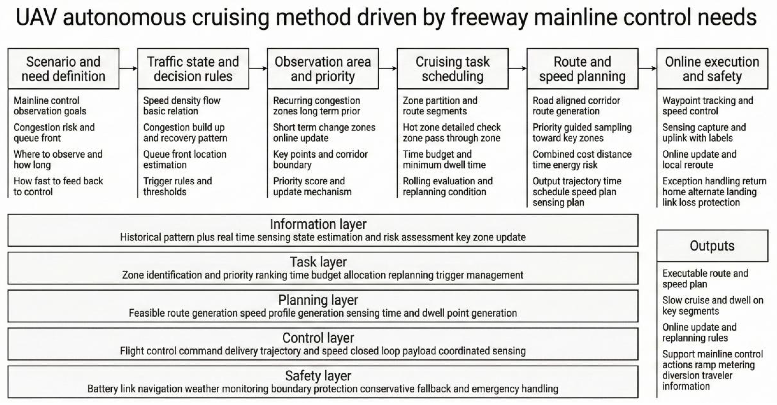
Figure 1 presents the technical roadmap of the UAV autonomous cruising method driven by expressway mainline control needs.
Figure 1.
Technical roadmap.
2. Expressway Mainline Control Requirements
Expressway mainline traffic control targets segments that exhibit recurrent congestion yet are not necessarily congested at all times. Controllers need to obtain the operating state of a segment before congestion forms, assess the risk of queue growth and queue-tail spillback, and determine the activation timing and effective scope of measures such as metering, diversion, and information guidance. Low-altitude UAVs can reach the area rapidly and maneuver flexibly; they can take off in advance during expected peak-congestion periods and collect state information above the mainline corridor to support judgments on whether congestion will occur, its impact range, and its duration. Accordingly, mainline control needs can be summarized into two types of outputs. The first is determining the potential impact range of concern and defining the upstream and downstream boundaries of the observation corridor. The second is establishing criteria for congested and near-congested states and specifying the traffic parameters to be measured.
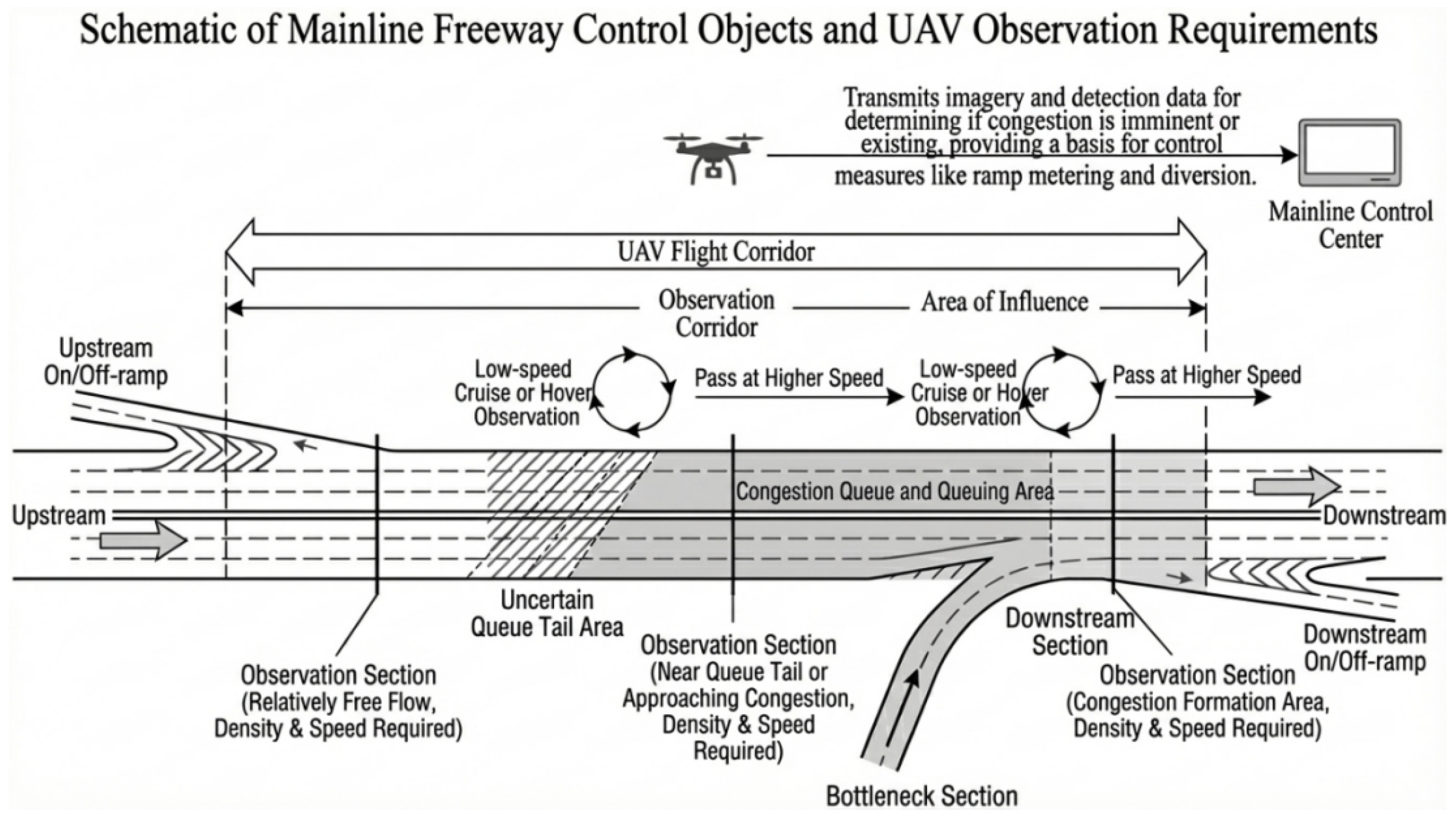
Mainline control focuses primarily on density and speed. Density indicates whether traffic is approaching saturation, while speed reflects whether operations have significantly deteriorated. Both can be inferred from nadir-view UAV imagery. Traffic volume is informative on short time scales, but it often requires stable observation windows and is therefore better treated as an auxiliary variable. Accordingly, observation demands concentrate on two executable tasks. The first task is defining criteria for congested and near-congested states so that measurable density and speed can be mapped to discrete operating levels and key observation segments can be marked. The second task is estimating, under given arrival and discharge conditions, the maximum possible queue length and the potential impact range so as to determine the mainline interval that the UAV should cover and to align the observation-corridor boundaries with actual entrances and exits [23]. Figure 2 illustrates the expressway mainline control targets and the corresponding UAV observation demands considered in this study.
Figure 2.
Schematic of expressway mainline control targets and UAV observation demands.
Observation–demand modeling is based on the macroscopic triangular fundamental diagram and kinematic-wave theory [24]. Let the local density be , the flow rate be q, the jam density be , the free-flow speed be , and the congestion wave speed be w; then the fundamental diagram can be written as
Accordingly, the critical density and capacity are obtained as
Between free-flow and congested states, the queue-tail shockwave speed is given by the Rankine–Hugoniot condition as
where and correspond to the upstream arrival state, and and correspond to the state determined by downstream discharge capacity. Using the mainline arc-length coordinate s to represent location, let the bottleneck or key control point be at , and given the prediction horizon T. When , the queue spills back upstream; its maximum possible length within the time window is
Accordingly, the predicted queue-tail position can be obtained as . The possible range of the short-term queue-tail front is denoted as , and a fixed-length buffer around the queue-tail position is constructed as
where is the uncertainty buffer distance of the front. The speed constraint induced by is taken as a piecewise-constant value
where is the low-speed observation speed near the queue tail.
State identification requires converting congestion and near-congestion into decision rules with density and speed as variables. Based on the triangular fundamental diagram, a segment satisfying or can be classified as congested, where is the speed threshold consistent with the congested branch. Near-congestion characterizes the early stage of queue-tail formation and growth; a segment satisfying and exhibiting a persistent increase in density or a persistent decrease in speed can be classified as near-congested, where is the warning density threshold. According to these rules, the operating level at any mainline point can be determined by the density–speed combination, and segments can be labeled as potential bottlenecks, key segments near the queue tail, or relatively stable passing segments [25].
The spatial heterogeneity of recurrent congestion along the mainline is characterized by a longitudinal prior function , where s denotes the arc-length coordinate along the mainline. It integrates historical congestion frequency and duration to describe long-term structural risk and to derive segment-wise speed policies. Let the baseline speed upper bound be , the system speed limit be , and the low-speed intensity parameter be . The longitudinal speed upper bound is defined as
The allowable speed is
In this way, the speed upper bound is automatically tightened in long-term high-risk segments and near the short-term front to support low-speed observations and short loitering, while a higher cruising speed is maintained in stable segments to improve endurance utilization.
3. UAV Cruise Path Planning
To translate time- and position-level observation demands into an executable cruise trajectory and speed profile, the UAV is required to fly efficiently along the mainline alignment and to form stable low-speed observations in high-risk recurrent-congestion arc segments and near the front. For convenience, denote the determined observation-corridor boundaries and the flyable area by , and denote the no-fly zones and obstacle areas defined by maps and control requirements by . The planning output is a trajectory , which satisfies geometric constraints and speed constraints , where is the arc-length projection of the trajectory onto the mainline centerline.
Sampling-based planners such as the rapidly exploring random tree (RRT) provide an efficient way to explore feasible paths under obstacle and corridor constraints [26].
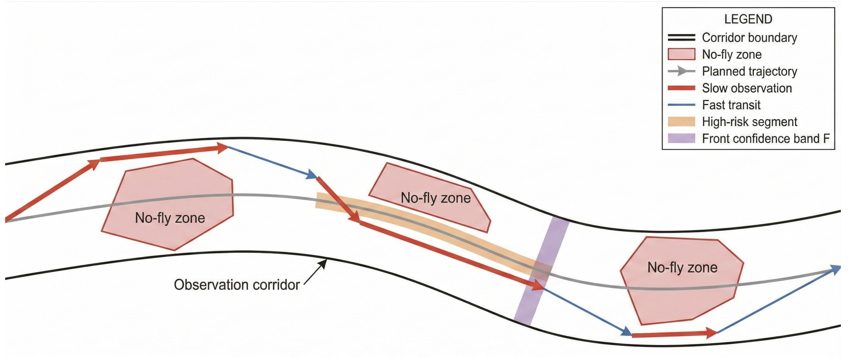
For path generation, a CLG-TP-RRT* method is adopted. It introduces mainline-centerline guidance into the RRT* random-sampling tree framework so that sampled points and tree nodes preferentially extend along the mainline direction during expansion and rewiring. This reduces ineffective lateral growth within the corridor cross section and improves alignment with the mainline geometry. For any sampled point x, its centerline arc-length coordinate is obtained by projection , and a distance metric with different weights along the longitudinal and lateral directions is used in nearest-neighbor search and rewiring to ensure geometric consistency with the mainline within the feasible domain [27]. Figure 3 provides a schematic of the UAV cruise path planning process adopted in this study.
Figure 3.
Schematic of UAV cruise path planning.
The sampling strategy directly incorporates long-term risk and short-term front information into the sampling probability to improve coverage efficiency of key arc segments. The sampling distribution is set as
where is the base random term, controls the bias strength toward high-risk recurrent-congestion arc segments, controls the bias strength toward the vicinity of the front confidence band, and is an indicator function. Without sacrificing global exploration capability, this setting enables the tree to form feasible connections faster in high-risk arc segments and near the front band .
Informed sampling variants such as Informed RRT* show that focusing samples within an admissible heuristic region can accelerate convergence, which inspires heuristic focusing under corridor constraints [28].
Edge cost uses a time-based metric, ensuring consistency between path search and the allowable-speed function. For any edge e, the cost is defined as
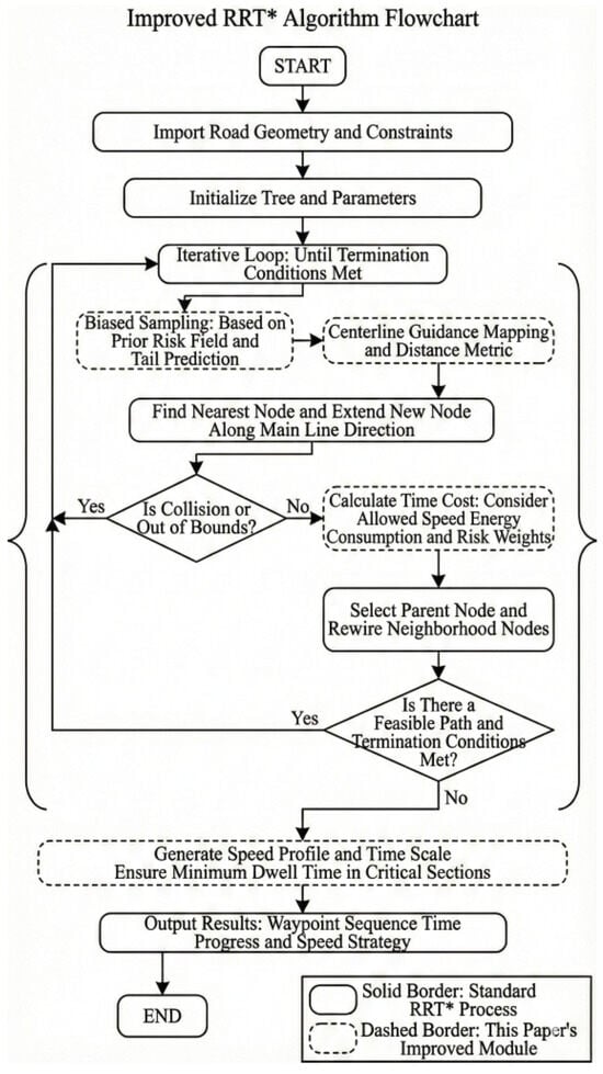
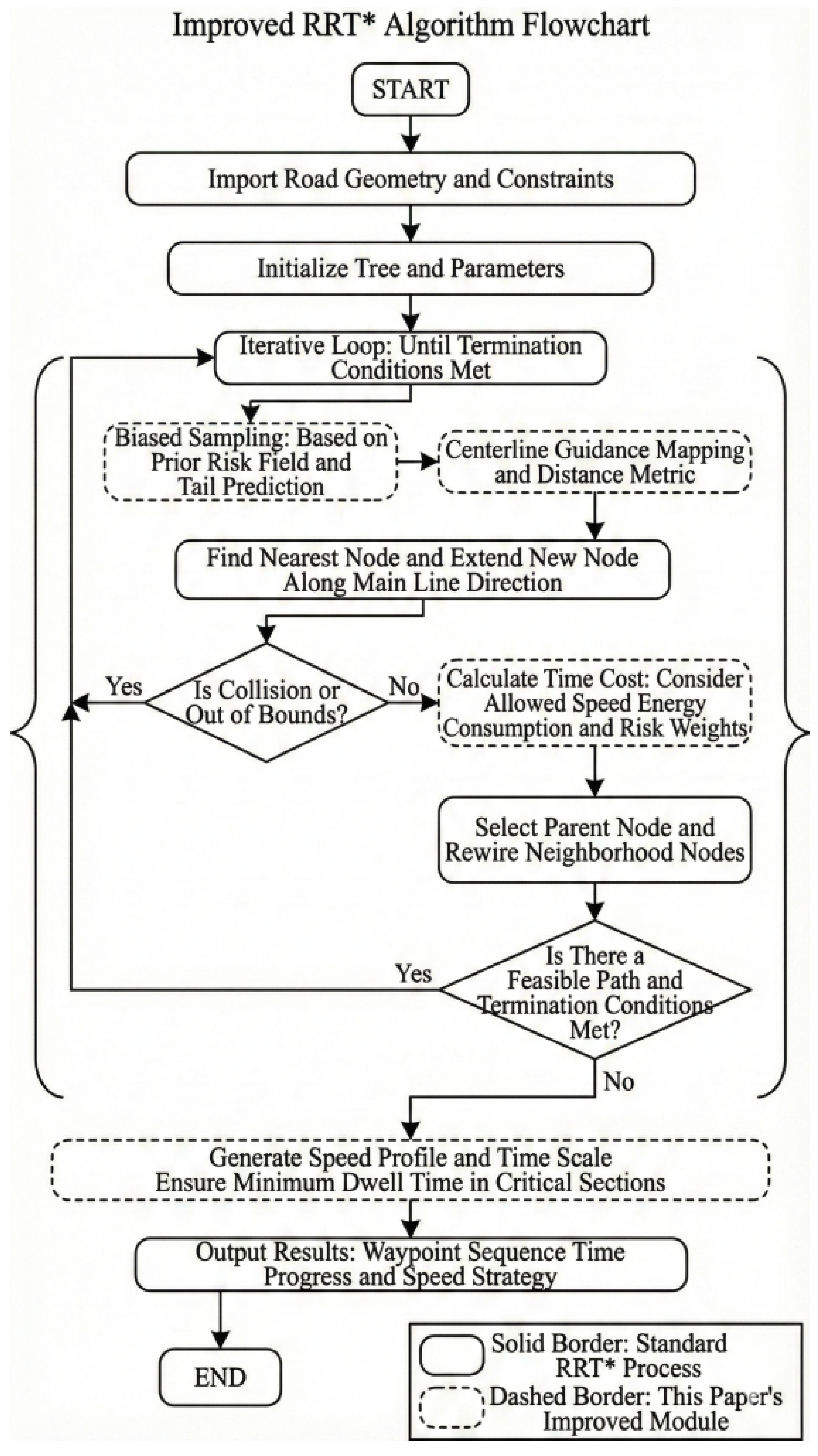
which explicitly converts differences in speed upper bounds across arc segments into differences in time cost. Consequently, key segments naturally obtain higher time weights due to lower allowable speeds. After the path is generated, a speed profile is constructed along the final trajectory using arc-length parameterization and satisfies . A stable observation speed is used within key segments, and smooth acceleration/deceleration is applied at segment boundaries to ensure speed continuity, thereby producing a waypoint sequence, time scale, and speed profile that can be directly used for autonomous flight execution. Figure 4 summarizes the CLG-TP-RRT* algorithm as a flowchart.
Figure 4.
Flowchart of the CLG-TP-RRT* algorithm.
From a computational perspective, CLG-TP-RRT* follows the standard RRT* loop of sampling, nearest neighbor search, steering, collision checking, and rewiring. With a balanced spatial index such as a kd tree, nearest neighbor and neighborhood queries have expected complexity for n nodes, and the overall expected complexity for n samples is for the search operations, while a naive implementation can degenerate toward in the worst case. Centerline guidance adds a projection and an anisotropic metric evaluation per query, which is , and the time-metric edge cost evaluation is when is represented as a piecewise function along s. Therefore, the asymptotic order is consistent with RRT*, and the main effect is on constant factors.
4. Automated Implementation of UAV Flight Missions
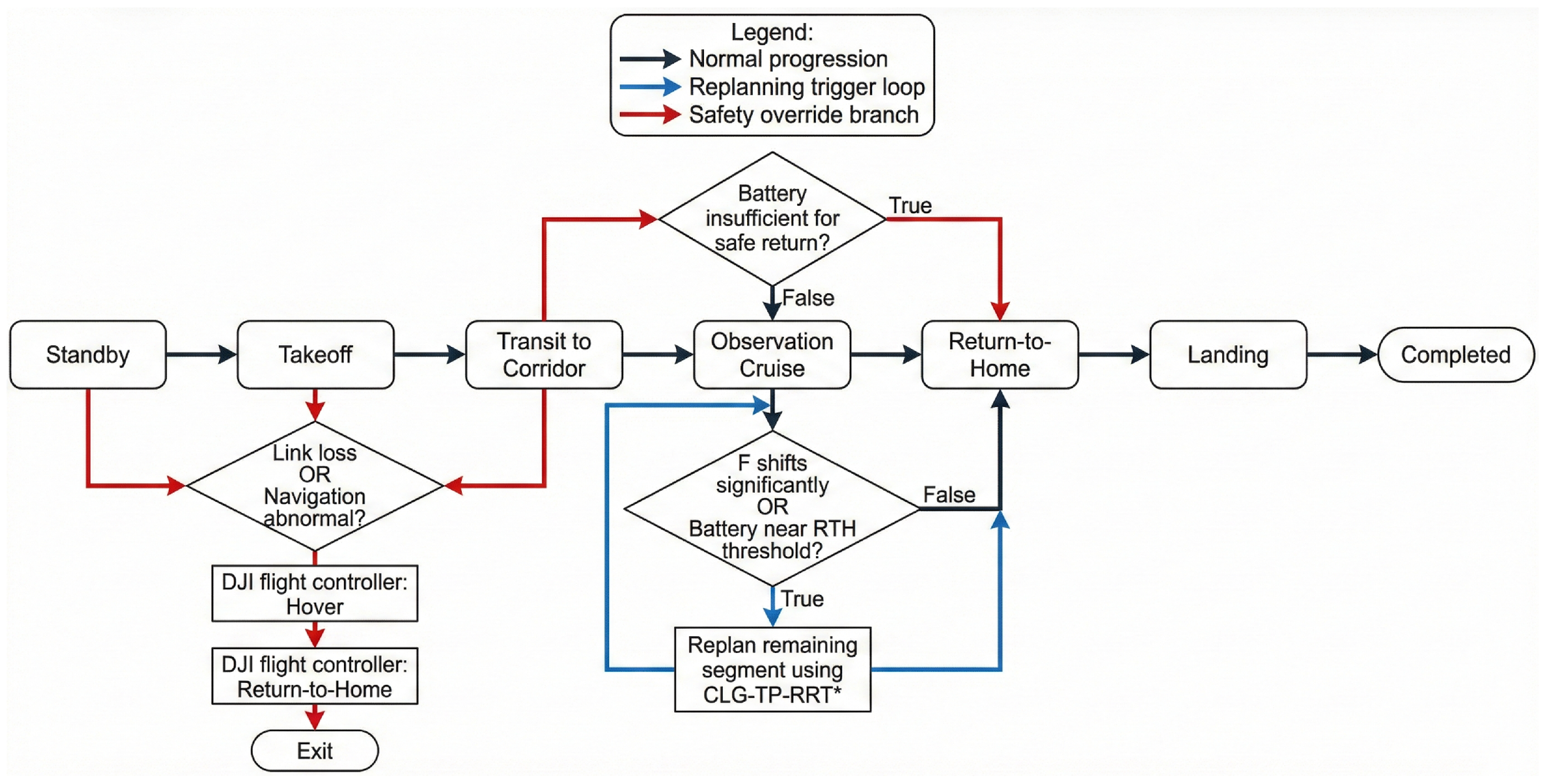
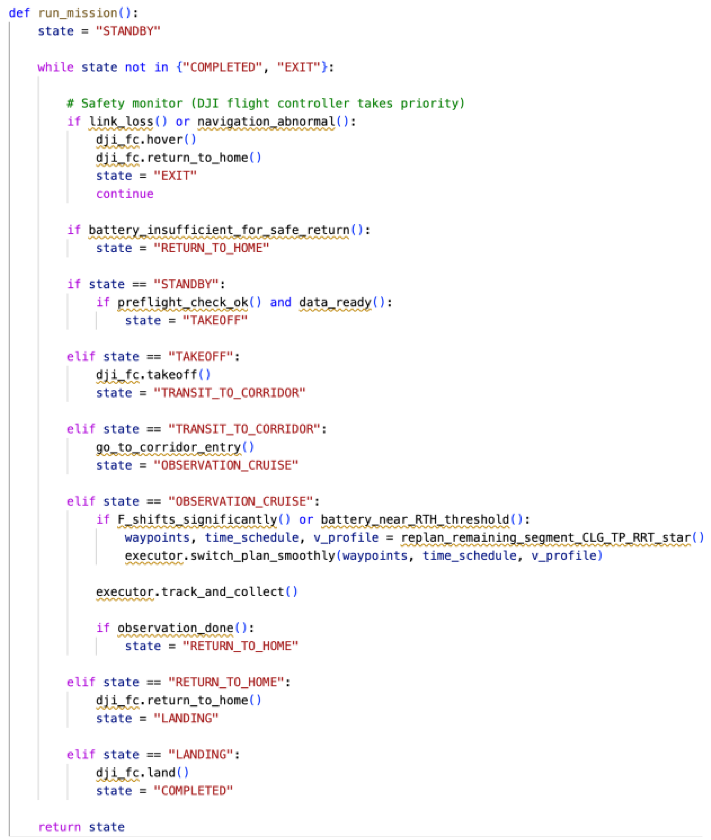
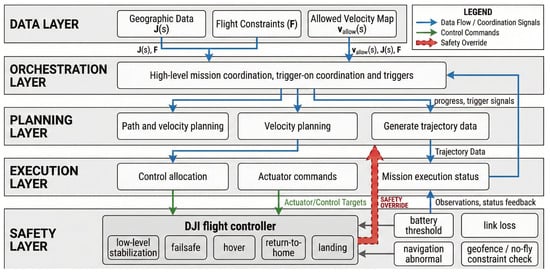
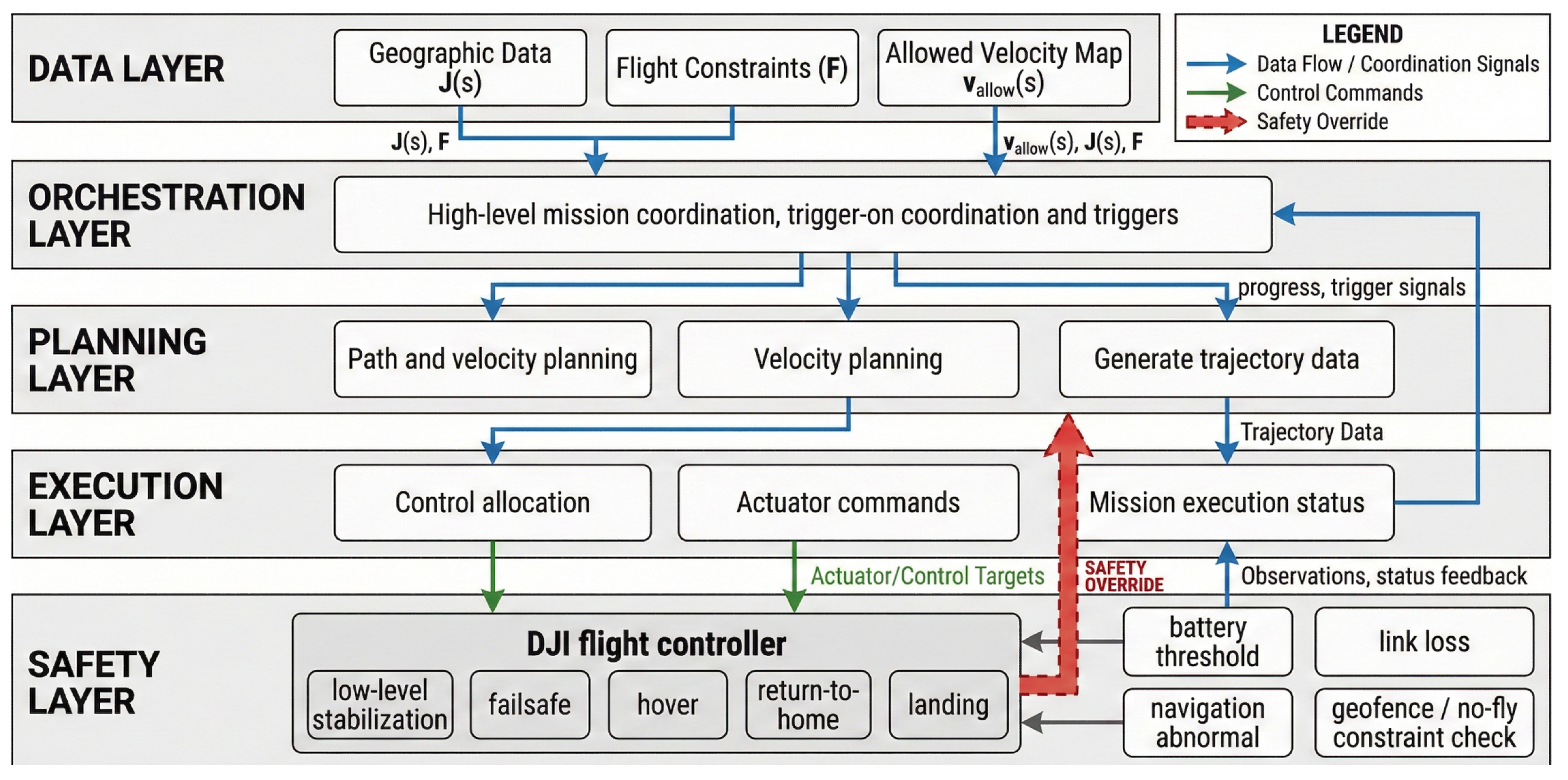
The automated implementation framework for UAV flight missions adopts a hierarchical structure consisting of a data layer, an orchestration layer, a planning layer, an execution layer, and a safety layer, and tasks run in a rolling manner under a unified state machine. The workflow design and pseudocode are shown in Figure 5 and Figure 6.
Figure 5.
Workflow of automated UAV flight missions.
Figure 6.
Pseudocode of automated UAV flight missions.
The data layer organizes historical statistics, roadside detections, and onboard observations into unified mainline arc-length-coordinate data and maintains the prior function , updating it based on real-time observations and forecasts and , providing consistent inputs for task orchestration and path planning. According to the mission endurance budget and remaining battery, the orchestration layer consolidates the observation-corridor boundaries and low-speed demands of key arc segments into a task description and sets triggers for online replanning. Trigger events mainly include drift, remaining battery approaching the return-to-home threshold, and communication/navigation anomalies. Under feasible-space constraints , the planning layer calls CLG-TP-RRT* to generate a waypoint sequence that satisfies as well as the time scale and speed profile , and performs rolling updates only for the remaining flight segments when replanning is triggered. The execution layer converts the waypoint sequence and time scale into trackable spatial reference trajectories and time–progress curves, sending position and speed targets to the autopilot, driving the payload to complete image acquisition and transmission according to segment strategies, and feeding deviations and abnormal states back to the orchestration and safety layers. At the bottom level, the safety layer relies on DJI flight-control functions such as attitude stabilization, fail-safe protection, and return-to-home capability to constrain planning and execution commands, continuously monitoring battery, link, navigation, and weather information, and checking the current trajectory against for boundary violations. When risks arise, it preferentially triggers hovering, return-to-home, or nearby emergency landing provided by the DJI flight controller, ensuring that the system still satisfies safety constraints under unexpected events. Figure 7 illustrates the layered architecture of the autonomous UAV cruise task.
Figure 7.
Layered architecture of the autonomous UAV cruise task.
The task state machine includes standby, takeoff, transfer, observation cruising, return, and landing. After a mission is created and parameters are loaded on the ground station, it enters standby. After pre-flight checks and environmental assessment pass, it enters takeoff, during which the autopilot performs takeoff and completes positioning and heading stabilization, followed by transfer to reach the entrance of the observation corridor. After entering observation cruising, the execution layer issues targets in a rolling manner according to the waypoint sequence and time scale and switches between low-speed observation and fast traversal based on the speed profile ; when significant drift occurs or the battery approaches the return-to-home threshold, the orchestration layer triggers replanning. The planning layer calls CLG-TP-RRT* to update the waypoint sequence, the time scale, and , and the execution layer smoothly switches to the new solution to continue cruising. When the observation-end condition is met or safety thresholds are triggered, the mission enters return, during which the autopilot returns and lands at the takeoff/landing site. If link interruption, navigation failure, or sudden weather changes occur at any stage, the safety layer takes over directly and switches to conservative strategies, terminating the mission and landing nearby if necessary.
5. Case Study
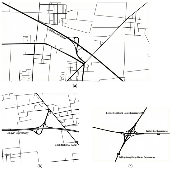
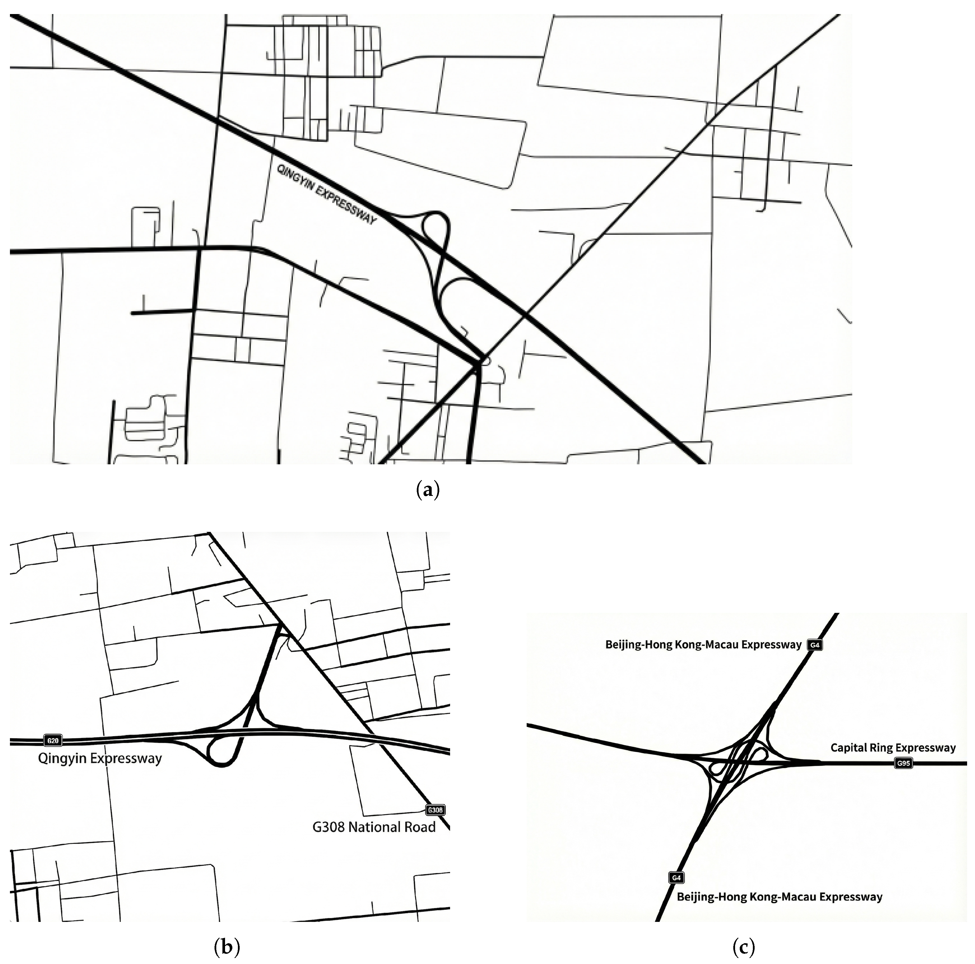
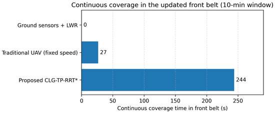
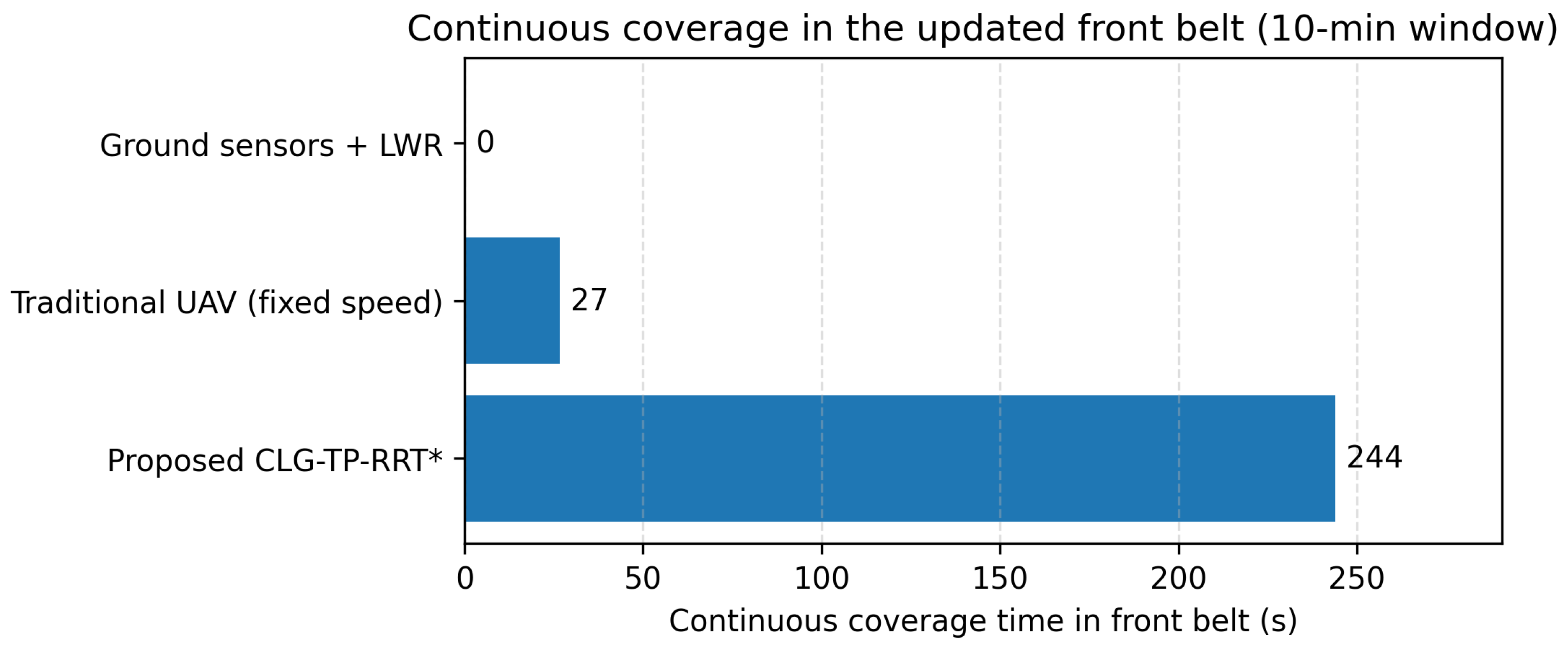
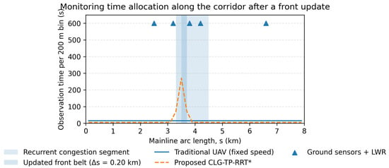
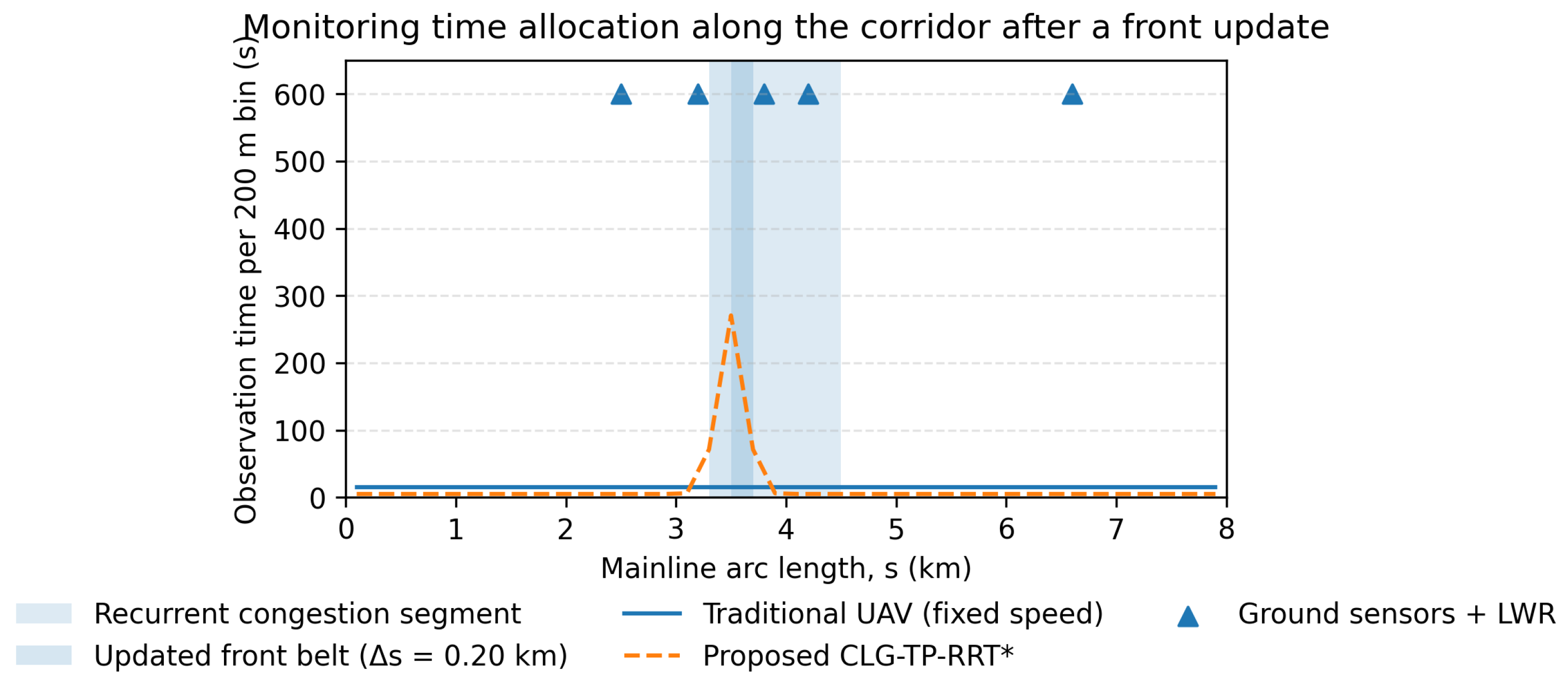
Recurrent congestion belts are frequently observed near interchanges and toll-station areas on expressway mainlines. Three representative scenarios with different corridor geometries and recurrent-congestion patterns are considered, as shown in Figure 8: Scenario S1 (Figure 8a) corresponds to the Zhaoxian interchange area on the Qingyin Expressway; Scenario S2 (Figure 8b) corresponds to a frequently congested segment near the Luancheng toll-station area on the Qingyin Expressway; and Scenario S3 (Figure 8c) corresponds to the Jingshi interchange between the Beijing–Hong Kong–Macau Expressway and the Capital Ring Expressway. For each scenario, sampling-based planners are executed in independent runs with different random seeds, and the mean and standard deviation of key metrics are reported, while the ground-sensor scheme and the traditional fixed-speed cruise are deterministic under the same settings. Table 2 lists the key parameters and configuration used in the case study. Figure 9, Figure 10, Figure 11 and Figure 12 present the results for Scenario S1, and Table 3 summarizes the quantitative comparison across all scenarios. Unless otherwise stated, the common model and algorithm parameters follow Table 2.
Figure 8.
Schematic road networks of three representative expressway scenarios used for validation. (a) Zhaoxian segment, Qingyin Expressway. (b) Luancheng toll-station area, Qingyin Expressway. (c) Jingshi interchange, Beijing–Hong Kong–Macau Expressway.
Table 2.
Key parameters and configuration in the case study.
Figure 9.
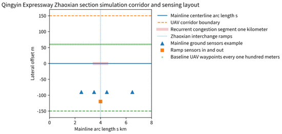
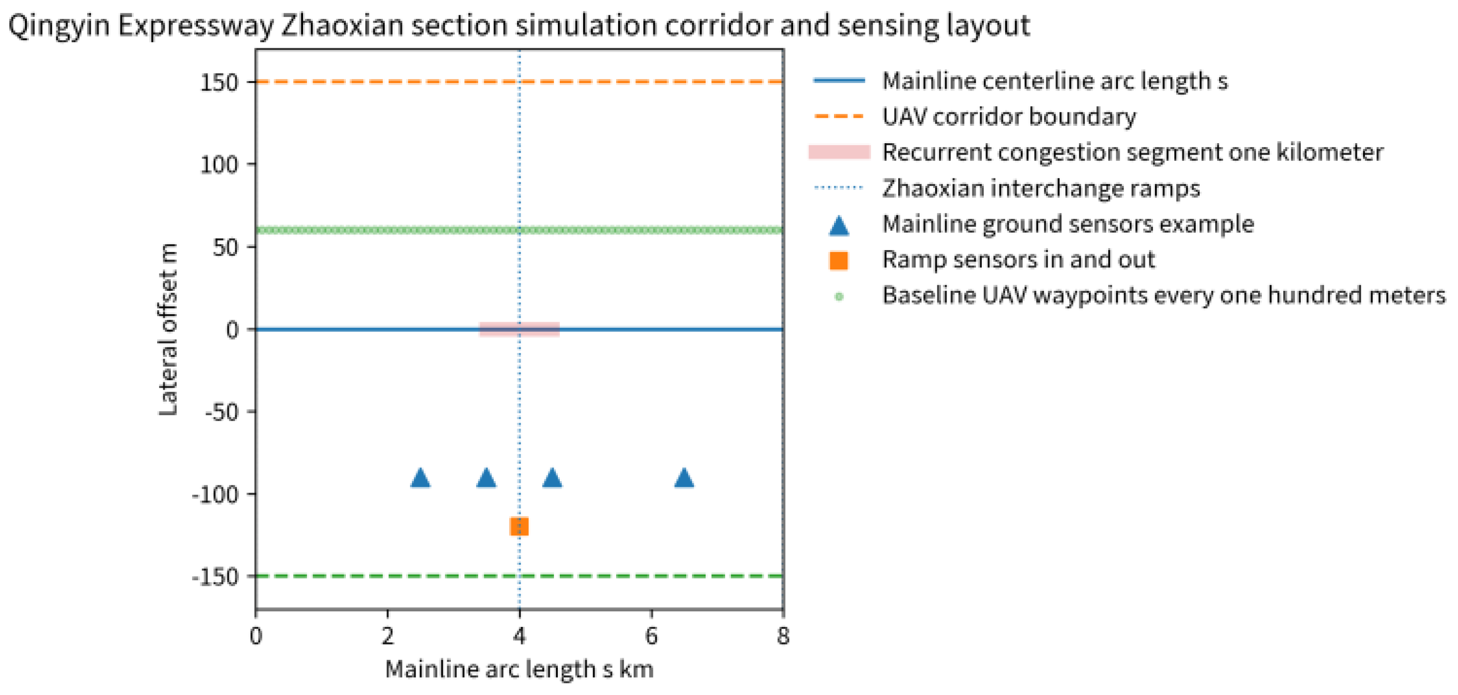
Recurrent congestion belt and monitoring layout on the Zhaoxian segment of the Qingyin Expressway.
Figure 10.
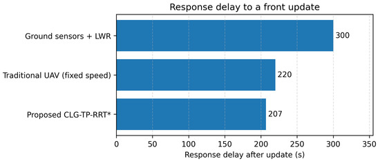
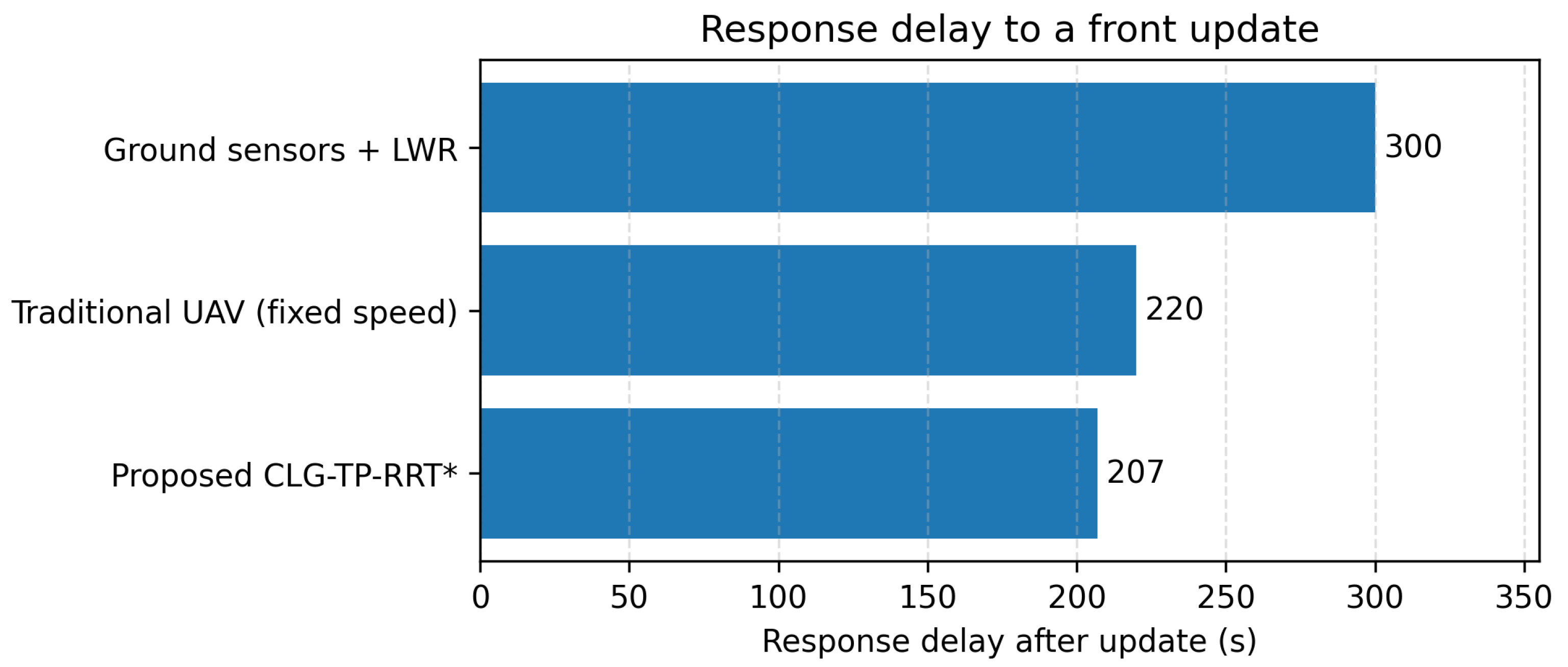
Response delay to a front update among the three methods (Scenario S1).
Figure 11.
Continuous coverage time of the front belt among the three methods (Scenario S1).
Figure 12.
Distribution of observation time along the mainline within 10 min after the update (Scenario S1).
Table 3.
Multi-scenario quantitative comparison of response delay and front-belt continuous coverage (mean ± std; repeated planning runs for sampling-based methods).
In Scenario S1 (Qingyin Expressway Zhaoxian segment in Hebei Province), a stable recurrent congestion belt exists near the interchange, and the typical congested length is about 1 km. An arc-length coordinate s is defined along the mainline. The upstream end of the analysis corridor is set to , and the driving direction is taken as the positive s direction. The corridor length is km. The alignment point of the Zhaoxian interchange is located at km, and the recurrent congestion belt is within km.
The prior function represents the longitudinal pattern of recurrent congestion and can be obtained from historical speed and density series projected onto s and normalized. In this case study, is represented by a piecewise profile that assigns within km and applies linear transitions within km and km.
The short-horizon front band is updated using the kinematic-wave relationship. Fundamental-diagram parameters are set as , , and . The upstream arrival is . The discharge is before the update and after the update. The prediction window is . The update trigger time is , and the effective update on the ground side lags to . The half-width of the front belt is set to for the ground scheme and for the UAV scheme. For segment labeling in the observation–demand model, a speed threshold of is adopted, and the warning density is set as .
For the traditional UAV scheme, waypoints are placed every 100 m along the centerline, and the UAV cruises at a constant speed of . For the proposed method, , , , and are used to construct . The biased sampling parameters are set as , , and . Loitering is applied within the front belt, with a duration of 120 s before the update and 180 s after the update to concentrate observation time on the high-value segment after the update. Two stronger baselines are included. The standard RRT* baseline uses uniform sampling and the Euclidean metric within the same corridor. The adaptive replanning baseline (Ref. [22]) updates its waypoint organization toward the updated front but maintains a fixed cruise speed (i.e., without tightening inside the front belt). The parameter settings are summarized in Table 2.
For Scenario S2, the corridor length is set to km, and the recurrent congestion belt is within km, which is consistent with the congested area influenced by the toll-station operations; the updated front belt is centered at km with m for the UAV scheme. The upstream arrival is , and the discharge changes from to after the update. For Scenario S3, the corridor length is km, and the recurrent belt is within km; the updated front belt is centered at km with m for the UAV scheme. The upstream arrival is , and the discharge changes from to after the update. Other settings follow Scenario S1.
Figure 9 shows the location of the Zhaoxian interchange, the recurrent congestion segment, and the sensing conditions of the three methods under the s coordinate. The three methods are compared within the same corridor and under the same background. The ground-based scheme relies on discrete measurement points and performs LWR analysis accordingly; the traditional UAV scheme forms a fixed cruising organization using evenly spaced waypoints along the centerline; and the proposed method synchronously adjusts subsequent flight organization and speed allocation after the short-term front update so that the updated information can be directly converted into executable spatial migration and temporal reallocation.
Two metrics are used to quantify the effectiveness of a front update. The response delay is defined as , where s denotes the front-update event time, and denotes the earliest time at which the method can provide an observation within the updated front belt. For the ground-sensor scheme, corresponds to the time when the updated front estimate becomes available after the processing pipeline; for UAV schemes, is the first time the UAV enters the updated belt after the update and any replanning maneuver. The continuous coverage time is defined as the longest uninterrupted time spent inside the updated front belt within the 10 min window after .
Figure 10 compares the response delay after a front update. Due to processing lag, the ground sensor + LWR scheme shows an effective response delay of 300 s after the event; in the traditional UAV scheme with uniformly spaced waypoints and constant-speed cruising, a hit depends on the spatiotemporal coincidence between the trajectory and the updated front, resulting in a delay of 220 s. After the update is triggered at s, the proposed method reallocates subsequent flight segments toward the updated front through online replanning and proactively decelerates and turns under the constraint, reducing the delay to 207 s. This result indicates that once front drift occurs, the proposed method is more likely to yield timely and consistent responses rather than relying on the chance of a cruise trajectory passing by.
Figure 11 compares the continuous coverage time of the front belt within 10 min after the update. The ground-based scheme is dominated by point observations and cannot form continuous coverage over the front belt, yielding a continuous coverage time of 0 s. The traditional constant-speed UAV cruising scheme stays for a limited time near the front belt, resulting in 27 s of continuous coverage. In the proposed method, slow-speed observation is formed within the front belt under the constraints of and , and loitering is superimposed, increasing the continuous coverage time to 244 s. This improvement indicates that the advantage lies primarily in coverage quality rather than merely in reachability; limited endurance can be converted more reliably into sustained observation within the front belt, thereby strengthening the evidence for assessing queue spillback risk and the affected range.
Figure 12 presents the distribution of observation time projected along s within 10 min after the update. The lightly shaded band indicates the recurrent congestion segment, and the darker band indicates the updated front belt and corresponds to the UAV scheme with m. The ground-based scheme provides stable information at several fixed points but lacks spatial continuity. The observation time distribution of the traditional constant-speed UAV cruising scheme is relatively scattered and fails to maintain a stable focus on the updated front. By contrast, the proposed method forms a pronounced time concentration near the updated front belt, reflecting that online replanning actively migrates the observation budget toward the new front, while and the loitering mechanism ensure that time can stay in high-value segments rather than being consumed by uniform-speed traversal, thereby achieving higher coverage density and stronger continuous tracking capability within the same time window.
Generality beyond Scenario S1 is assessed on Scenarios S2 and S3. Table 3 reports the response delay to a front update and the continuous coverage time within the updated front belt for five methods, including the standard RRT* planner and the adaptive replanning baseline (Ref. [22]) (mean ± std; repeated planning runs for sampling-based methods). Across the three scenarios, the proposed method consistently reduces response delay compared with the traditional cruise scheme, and its main advantage lies in forming substantially longer continuous tracking within the front belt.
In Table 3, Table 4, Table 5 and Table 6, several continuous-coverage standard deviations appear as 0.0. This is because, under the adopted s-parameterized execution, the time spent inside the belt is dominated by the prescribed in-belt speed bound and the fixed loitering schedule once the belt is reached; the remaining seed-to-seed variation is below the reporting precision and is rounded to 0.0.
Table 4.
Ablation study in Scenario S1 (mean ± std; ).
Table 5.
Sensitivity analysis of key parameters in Scenario S1 for the proposed method (mean over runs; one-at-a-time perturbation).
Table 6.
Robustness evaluation in Scenario S1 under wind disturbances, communication latency, and front localization/prediction errors (mean ± std; ).
The contribution of centerline guidance, the time-metric edge cost, and biased sampling is isolated through an ablation study in Scenario S1, where each component is removed while keeping other settings unchanged. Table 4 shows that centerline guidance contributes primarily to reducing response delay, the time metric improves the time allocation toward the updated front, and biased sampling stabilizes the response across repeated runs; removing all three components recovers the standard RRT* baseline.
Sensitivity of the proposed method to key parameters is further examined. Specifically, the triangular fundamental-diagram parameters , the speed-policy and belt parameters , the sampling weights , and the congestion threshold are perturbed by (one-at-a-time) in Scenario S1. Table 5 summarizes the mean response delay and continuous coverage time. The results indicate that the proposed method is relatively insensitive to moderate perturbations in traffic-flow parameters and weights, while the front-belt half-width and the in-belt speed have the most direct impact on the achievable continuous tracking time.
Robustness under practical disturbances is also evaluated, including wind-induced airspeed degradation, communication latency, and front localization/prediction errors. Table 6 shows that the proposed method degrades gracefully: communication latency primarily shifts the response delay, wind increases response delay and reduces continuous coverage through reduced airspeed, and localization errors mainly reduce the effective continuous tracking inside the front belt.
Representative faults (navigation failures, GPS drift, communication loss, and sudden weather changes) are injected, and the safety module response is recorded. Table 7 reports the activation and interruption times.
Table 7.
Logic-level fault-injection safety-response stress tests in Scenario S1 (proposed method; monitoring cycle 1 s).
These tests follow a deterministic fault-injection protocol in the mission state machine. The activation times are quantized by the 1 s monitoring cycle, and the recovery/interruption times correspond to configured timeouts (e.g., bounded hold durations for re-localization or link recovery). Under these defined envelopes, the success rate indicates whether the safety layer switches the vehicle into the intended conservative mode and completes recovery or safe termination.
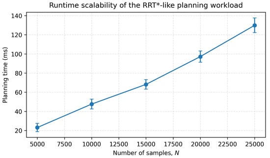
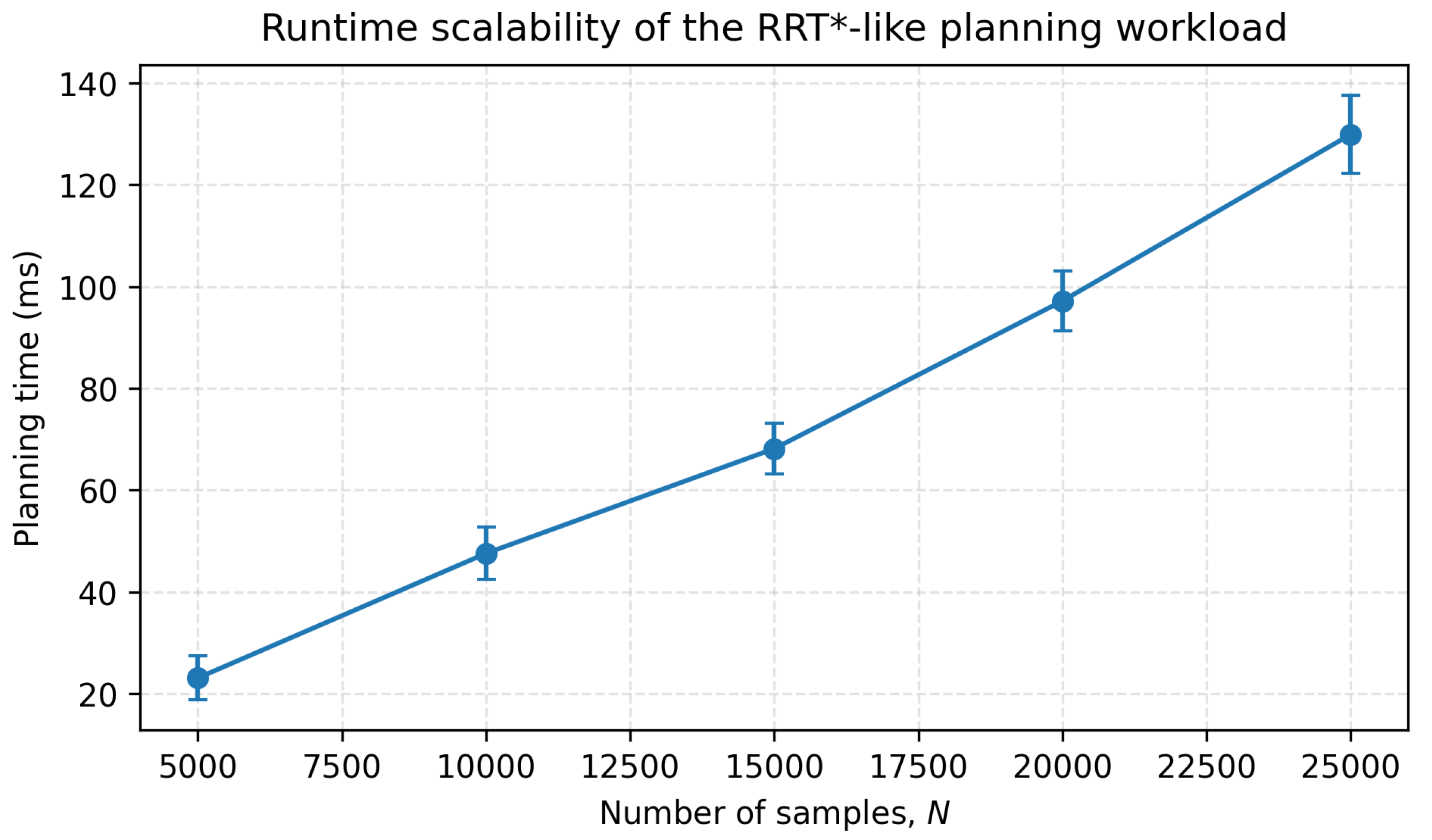
Finally, the computation time of initial planning and online replanning is reported for the sampling-based methods in the prototype implementation. Table 8 lists the measured times along with the sample budgets used for each planner. Since runtime grows with the number of samples, dividing the mean times by the corresponding sample counts gives comparable costs on a per-sample basis (init: 54.1/51.5/48.9 ms per samples for standard RRT*, adaptive replanning, and CLG-TP-RRT*; replan: 50.4/48.9/47.1 ms per samples, respectively). Figure 13 further shows the scaling with the sample budget in an RRT*-like neighbor-search workload.
Table 8.
Computation time for initial planning and replanning (mean ± std; ).
Figure 13.
Runtime scalability of the RRT*-like planning workload used for computation-time reporting.
6. Discussion
The response-delay reduction is modest because the front update becomes effective after a non-negligible ground-side processing lag (300 s), and all methods still need to traverse essentially the same physical distance to reach the updated front belt. As shown in Table 3 and Table 4, CLG-TP-RRT* shortens the response delay by about 6% (approximately 9–22 s across Scenarios S1–S3) relative to the traditional fixed-speed UAV baseline. Compared with the standard RRT* planner and the adaptive replanning baseline (Ref. [22]), the gains primarily come from coupling the front update with both centerline-guided exploration and in-belt speed tightening, which reallocates monitoring time toward the updated belt rather than only relocating waypoints. Therefore, the more pronounced benefit is in tracking quality: the method consistently forms longer continuous coverage within the front belt, which is valuable when the front evolves over time and the monitoring window is limited.
Although components such as centerline guidance, biased sampling, and time-based costs are individually known in sampling-based motion planning, the present formulation couples them with a traffic-demand model (recurrent belt and short-horizon front) and an arc-length speed policy so that online replanning reallocates monitoring time toward an evolving front belt under corridor and speed constraints. This coupling targets expressway-mainline control requirements, where the objective is sustained, front-aware coverage rather than geometric shortest paths.
The observation–demand model adopts a triangular fundamental diagram and kinematic-wave logic to produce a tractable front-belt estimate and a longitudinal priority field. These macroscopic assumptions are appropriate when the corridor exhibits a dominant longitudinal bottleneck and the control objective emphasizes queue-tail spillback and its immediate impact range. In mixed traffic or in segments with strong lane-changing effects, the lane-level behavior is aggregated into effective macroscopic parameters, so calibration of and thresholds becomes more important. Multi-bottleneck interactions and complex corridor geometries may yield multiple fronts or fragmented congestion patterns; in such cases, the framework can accommodate richer estimators by updating the front band (e.g., multiple belts or a probabilistic belt map) and the prior field without changing the planning loop.
Parameter configuration is designed to be scenario-transferable rather than purely manual. The recurrent belt and can be obtained by projecting historical speed/density series onto the arc-length coordinate and normalizing congestion frequency and duration. The front-belt half-width can be set from the combined uncertainty of front localization and communication/processing latency, while and are bounded by local regulations and sensing requirements for stable imaging. The one-at-a-time sensitivity test in Table 5 indicates that the delay/coverage metrics are relatively insensitive to moderate perturbations of traffic-flow parameters and sampling weights, whereas and directly affect the achievable continuous tracking time. In practice, calibration of , conservative selection of , and subsequent tuning of against the robustness protocol in Table 6 provide a repeatable workflow for new corridors.
Robustness to disturbances and prediction errors is summarized in Table 6. Communication latency primarily shifts response delay in an approximately additive manner, while wind-induced airspeed degradation increases response delay and slightly reduces belt adherence. Front localization/prediction errors can noticeably reduce continuous coverage when the front estimate becomes noisy. The current prototype uses an s-parameterized speed profile with smooth acceleration/deceleration at segment boundaries; therefore, the commanded profile is consistent with bounded speed transitions, but explicit acceleration/turn-rate limits are not yet optimized. These limits can be incorporated by constraining the steering step and by adding dynamic feasibility terms to the edge cost, while the same disturbance protocol can be retained for verification.
Communication and computation requirements are compatible with online replanning. The front updates and replanning outputs (updated belt parameters, waypoint sequence, and speed schedule) are lightweight compared with the video stream, so they can be transmitted at a low rate with timestamps, while latency manifests as the additive delay observed in Table 6. On the computation side, the prototype implementation reports sub-100 ms initial planning and sub-60 ms replanning times for the proposed method (Table 8), and Figure 13 shows the expected scaling with the sample budget in an RRT*-like neighbor-search workload. Safety responses under representative adverse conditions (Table 7) indicate that conservative fallback behaviors can be integrated without destabilizing the monitoring process, which supports integration with corridor geofencing and routine operational procedures. In deployment, compliance with low-altitude airspace regulations and coordination with existing traffic management workflows remain prerequisites; richer trajectory optimizers (e.g., energy-aware multi-criteria or MPC-based planners) can be introduced in the planning layer when consistent dynamic and energy models are available.
7. Conclusions
This study addresses key issues of mainline observation and presents an end-to-end procedure from observation–demand modeling to joint planning of path and speed and further to automated execution. The observation–demand model converts long-term congestion and short-term fronts into computable priorities and speed constraints, and the planning strategy centers on centerline guidance and time-based metrics to generate trajectories and speed profiles that balance efficiency and information-gathering quality, while the hierarchical execution system links data, orchestration, planning, execution, and safety into a closed loop, enhancing deployability and controllability.
This work still has limitations. The evaluation focuses mainly on a typical corridor and a single UAV and needs to be extended in terms of scenario diversity, disturbance intensity, and coupling with in-route control measures. Future work will validate the approach for multi-UAV cooperation, complex corridors, and multi-source sensing conditions and will refine parameter tuning and interface details in field applications to promote integration with mainline control systems.
Author Contributions
Conceptualization, W.L. and Y.Y.; Methodology, W.L. and Y.Y.; Software, W.L. and Y.Y.; Validation, Y.Y.; Formal analysis, W.L. and Y.Y.; Investigation, W.L. and Y.Y.; Resources, G.L.; Data curation, W.L.; Writing—original draft, Y.Y.; Writing—review & editing, W.L. and G.L.; Visualization, W.L.; Supervision, G.L.; Project administration, W.L. All authors have read and agreed to the published version of the manuscript.
Funding
This research was funded by Key R&D projects in Guangxi (AB24010221, AB24010124).
Data Availability Statement
The original contributions presented in this study are included in the article. Further inquiries can be directed to the corresponding author(s).
Conflicts of Interest
The authors declare no conflict of interest.
References
- Lighthill, M.J.; Whitham, G.B. On kinematic waves. II. A theory of traffic flow on long crowded roads. Proc. R. Soc. Lond. A 1955, 229, 317–345. [Google Scholar] [CrossRef] [Scilit]
- Richards, P.I. Shock waves on the highway. Oper. Res. 1956, 4, 42–51. [Google Scholar] [CrossRef] [Scilit]
- Papageorgiou, M.; Hadj-Salem, H.; Blosseville, J.-M. ALINEA: A local feedback control law for on-ramp metering. Transp. Res. Rec. 1991, 1320, 58–64. [Google Scholar]
- Papageorgiou, M.; Kosmatopoulos, E.; Papamichail, I. Effects of variable speed limits on motorway traffic flow. Transp. Res. Rec. 2008, 2047, 37–48. [Google Scholar] [CrossRef] [Scilit]
- Kanistras, K.; Martins, G.; Rutherford, M.J.; Valavanis, K.P. A survey of unmanned aerial vehicles (UAVs) for traffic monitoring. In Proceedings of the 2013 International Conference on Unmanned Aircraft Systems (ICUAS), Atlanta, GA, USA, 28–31 May 2013; pp. 221–234. [Google Scholar] [CrossRef] [Scilit]
- Butilă, E.V.; Boboc, R.G. Urban traffic monitoring and analysis using unmanned aerial vehicles (UAVs): A systematic literature review. Remote Sens. 2022, 14, 620. [Google Scholar] [CrossRef] [Scilit]
- Liu, H.; Ma, R. Sky’s-Eye Perspective: A Multidimensional Review of UAV Applications in Highway Systems. Appl. Sci. 2025, 15, 11199. [Google Scholar] [CrossRef] [Scilit]
- Obaid, L.; Hamad, K.; Al-Ruzouq, R.; Abu Dabous, S.; Ismail, K.; Alotaibi, E. State-of-the-art Review of Unmanned Aerial Vehicles and Artificial Intelligence for Traffic and Safety Analyses: Recent Progress, Applications, Challenges, and Opportunities. Transp. Res. Interdiscip. Perspect. 2025, 33, 101591. [Google Scholar] [CrossRef] [Scilit]
- Debnath, D.; Vanegas, F.; Sandino, J.; Hawary, A.F.; Gonzalez, F. A Review of UAV Path-Planning Algorithms and Obstacle Avoidance Methods for Remote Sensing Applications. Remote Sens. 2024, 16, 4019. [Google Scholar] [CrossRef] [Scilit]
- Luo, J.; Tian, Y.; Wang, Z. Research on Unmanned Aerial Vehicle Path Planning. Drones 2024, 8, 51. [Google Scholar] [CrossRef] [Scilit]
- Wu, Q.; Su, Y.; Tan, W.; Zhan, R.; Liu, J.; Jiang, L. UAV Path Planning Trends from 2000 to 2024: A Bibliometric Analysis and Visualization. Drones 2025, 9, 128. [Google Scholar] [CrossRef] [Scilit]
- Salvo, G.; Caruso, L.; Scordo, A.; Guido, G.; Vitale, A. Traffic data acquirement by unmanned aerial vehicle. Eur. J. Remote Sens. 2017, 50, 343–351. [Google Scholar] [CrossRef] [Scilit]
- Khan, M.A.; Ectors, W.; Bellemans, T.; Janssens, D.; Wets, G. Unmanned aerial vehicle-based traffic analysis: Methodological framework for automated multivehicle trajectory extraction. Transp. Res. Rec. 2017, 2626, 25–33. [Google Scholar] [CrossRef] [Scilit]
- Wang, L.; Chen, F.; Yin, H. Detecting and tracking vehicles in traffic by unmanned aerial vehicles. Autom. Constr. 2016, 72, 294–308. [Google Scholar] [CrossRef] [Scilit]
- Ke, R.; Li, Z.; Tang, J.; Pan, Z.; Wang, Y. Real-time traffic flow parameter estimation from UAV video based on ensemble classifier and optical flow. IEEE Trans. Intell. Transp. Syst. 2019, 20, 54–64. [Google Scholar] [CrossRef] [Scilit]
- Shan, D.; Lei, T.; Yin, X.; Luo, Q.; Gong, L. Extracting key traffic parameters from UAV video with on-board vehicle data validation. Sensors 2021, 21, 5620. [Google Scholar] [CrossRef] [Scilit] [PubMed]
- Khan, M.A.; Ectors, W.; Bellemans, T.; Janssens, D.; Wets, G. Unmanned aerial vehicle-based traffic analysis: A case study for shockwave identification and flow parameters estimation at signalized intersections. Remote Sens. 2018, 10, 458. [Google Scholar] [CrossRef] [Scilit]
- Kim, E.-J.; Park, H.-C.; Ham, S.-W.; Kho, S.-Y.; Kim, D.-K. Extracting vehicle trajectories using unmanned aerial vehicles in congested traffic conditions. J. Adv. Transp. 2019, 2019, 9060797. [Google Scholar] [CrossRef] [Scilit]
- Kabashkin, I.; Kulmurzina, A.; Nadimov, B.; Tlepiyeva, G.; Sansyzbayeva, Z.; Sultanov, T. Traffic Monitoring Using UAV: Multi-Point Monitoring and Analysis. Drones 2025, 9, 370. [Google Scholar] [CrossRef] [Scilit]
- Popović, M.; Vidal-Calleja, T.; Hitz, G.; Chung, J.J.; Sa, I.; Siegwart, R.; Nieto, J. An informative path planning framework for UAV-based terrain monitoring. Auton. Robot. 2020, 44, 889–911. [Google Scholar] [CrossRef] [Scilit]
- Hollinger, G.A.; Sukhatme, G.S. Sampling-based robotic information gathering algorithms. Int. J. Robot. Res. 2014, 33, 1271–1287. [Google Scholar] [CrossRef] [Scilit]
- Yahia, C.N.; Scott, S.E.; Boyles, S.D.; Claudel, C.G. Unmanned aerial vehicle path planning for traffic estimation and detection of non-recurrent congestion. Transp. Lett. 2022, 14, 849–862. [Google Scholar] [CrossRef] [Scilit]
- Newell, G.F. A simplified theory of kinematic waves in highway traffic, part I: General theory. Transp. Res. Part B Methodol. 1993, 27, 281–287. [Google Scholar] [CrossRef] [Scilit]
- Daganzo, C.F. The cell transmission model: A dynamic representation of highway traffic consistent with the hydrodynamic theory. Transp. Res. Part B Methodol. 1994, 28, 269–287. [Google Scholar] [CrossRef] [Scilit]
- Treiber, M.; Kesting, A. Traffic Flow Dynamics: Data, Models and Simulation; Springer: Berlin/Heidelberg, Germany, 2013. [Google Scholar] [CrossRef] [Scilit]
- LaValle, S.M. Rapidly-Exploring Random Trees: A New Tool for Path Planning; Technical Report TR 98-11; Computer Science Department, Iowa State University: Ames, IA, USA, October 1998. [Google Scholar]
- Karaman, S.; Frazzoli, E. Sampling-based algorithms for optimal motion planning. Int. J. Robot. Res. 2011, 30, 846–894. [Google Scholar] [CrossRef] [Scilit]
- Gammell, J.D.; Srinivasa, S.S.; Barfoot, T.D. Informed RRT*: Optimal sampling-based path planning focused via direct sampling of an admissible ellipsoidal heuristic. In Proceedings of the IEEE/RSJ International Conference on Intelligent Robots and Systems (IROS), Chicago, IL, USA, 14–18 September 2014; pp. 2997–3004. [Google Scholar] [CrossRef] [Scilit]

Disclaimer/Publisher’s Note: The statements, opinions and data contained in all publications are solely those of the individual author(s) and contributor(s) and not of MDPI and/or the editor(s). MDPI and/or the editor(s) disclaim responsibility for any injury to people or property resulting from any ideas, methods, instructions or products referred to in the content. |
© 2026 by the authors. Published by MDPI on behalf of the World Electric Vehicle Association. Licensee MDPI, Basel, Switzerland. This article is an open access article distributed under the terms and conditions of the Creative Commons Attribution (CC BY) license.