


Abstract
Battery management systems must estimate state of health (SOH) early in a cell’s life. This study examines how much of the reported estimation accuracy depends on the measurement protocol rather than the estimator. A physics-based fade curve, Random Forest, XGBoost version 3.3.0, a physics-assisted hybrid and a gated recurrent unit are compared using leave-one-cell-out validation on four NASA PCoE cells over early-life windows of 20–100 cycles. Training and evaluation observations are both drawn from cycles 1 to W; therefore, the primary task is cross-cell SOH estimation within an observed window, not future-cycle forecasting. A separate temporal evaluation yields higher forecasting RMSE, by factors of 1.9–4.3 relative to in-window estimation. At 50 cycles, XGBoost achieves a pooled RMSE of 0.024 SOH units, compared with 0.044 for the fade curve. Removing the recorded discharge duration feature increases RMSE by 34%. In a separate diagnostic comparison, a single time-under-load feature achieves lower RMSE than the full nine-feature set. Neither the fade curve estimate nor cycle index improves XGBoost when added as a feature. On common SOH support, the increase in R2 with window length is attributable to the widening test target distribution. A comparative analysis of four variable-current cells provides complementary evidence.
1. Introduction
Lithium-ion batteries can degrade through cycling and calendar ageing. A key parameter monitored by a battery management system (BMS) is the state of health (SOH), commonly expressed as the ratio of current available discharge capacity to a reference or rated capacity. Reliable SOH estimates support maintenance planning, pack balancing and range or runtime estimation [1,2,3]. Manufacturing variability and dependence on temperature and usage profiles complicate SOH estimation. A further practical limitation is that a BMS or fleet operator may initially have access to only a short segment of a cell’s operating history [4,5].
Battery SOH estimation methods include physics-based or semi-empirical models and data-driven approaches. The parametric relationships of capacity fade (e.g., exponential or power law dependence on cycle count) can be fit using physics-based or semi-empirical modelling approaches and may provide interpretability and data efficiency; however, model performance may be dependent on the assumed degradation behaviour that represents the cell. The performance of data-driven prognostic models can depend on the size and diversity of the training data [6]. Machine learning approaches include feature-engineered tree ensembles [7] and other data-driven methods [8]. Prior work has shown that early-cycle signals can contain information useful for predicting later battery life before substantial capacity fade is apparent, although this evidence concerns cycle life prediction and should not be equated directly with SOH estimation in the present four-cell study [9]. Physics-informed approaches seek to combine physical knowledge with learned models [10,11,12,13].
A single question of practical interest is seldom studied directly within a family of models under the same evaluation regime: what is the relation between estimation accuracy and the quantity of early-life cycling data that is available? Answering it requires comparative studies on fully open data that hold the train/test split, the cross-validation scheme and the data window identical across model families, and that separate the contribution of the measurement protocol from that of the estimator.
The dataset used in this study is the open NASA Prognostics Center of Excellence (PCoE) battery dataset [14], comprising repeated charge, discharge and impedance measurements for four 18650-format lithium-ion cells (B0005, B0006, B0007 and B0018) tested at room temperature. Prior studies have investigated battery capacity and SOH estimation using data-driven models, including transformer-based capacity estimation [15,16]; these works provide methodological context, as every study used the same NASA subset. A comparative study of five modelling strategies is assessed by leave-one-cell-out cross-validation at the 20, 50 and 100 cycle windows. First, the study quantifies how much of the accuracy attainable on this benchmark derives from the constant current measurement protocol rather than from the estimator, using information-matched feature ablations. Second, it shows that the improvement in R2 commonly reported as a function of observation-window length can arise from the widening distribution of test targets and reports an evaluation on a common SOH support that separates the two effects. Third, it establishes that appending a scalar physics-derived estimate to a tree ensemble cannot improve it, whatever fade curve is used, and identifies the structural reason. Fourth, it distinguishes quantitatively between estimating SOH within an observed early-life window and predicting future SOH from early-life measurements.
The objectives of this study are as follows: (i) to quantify how much of the SOH estimation accuracy attainable on this benchmark derives from the constant current measurement protocol rather than from the estimator; (ii) to characterise how estimation accuracy depends on the quantity of early-life data available, holding the evaluation support fixed so that the comparison is not confounded by a changing test distribution; (iii) to compare five modelling approaches, namely an empirical physics-based fade curve, Random Forest, XGBoost, a physics-assisted hybrid and a compact GRU, under one identical leave-one-cell-out protocol, and to establish what a physics-derived input feature can contribute to a tree ensemble; (iv) to distinguish estimation of SOH within an observed early-life window from prediction of future SOH, and to quantify the difference; and (v) to state the limits that a four-cell, single-chemistry, single-temperature dataset places on the conclusions that can be drawn, together with the further work required before the framework could be applied in an operational battery management system.
The remainder of this paper is organised as follows: Section 2 reviews related work on physics-based, data-driven, hybrid and transfer learning approaches to SOH estimation, and on prior use of the dataset. Section 3 describes the dataset, the parsing and quality control procedure, the definition of the SOH ground truth and the leave-one-cell-out protocol. Section 4 sets out the engineered per-cycle features. Section 5 describes the five modelling approaches and the configuration of each. Section 6 reports and discusses the results, covering accuracy across models and early-cycle windows, accuracy as a function of available early-cycle data, evaluation on a common SOH support, the distinction between early-window estimation and future-cycle forecasting, prediction and residual behaviour, feature importance and the discharge duration ablation, the influence of per-cell cutoff voltage, sensitivity to modelling and feature extraction settings, the effect of input representation on the sequence model, the structural behaviour of physics-assisted feature integration, a companion variable-current evaluation, computational cost, remaining useful life, applicability to battery management systems, and the limitations of the study. Section 7 concludes.
2. Related Work
Some recent reviews overview the field of battery health monitoring and state estimation of electric vehicles and stationary electric storage, including physics-based and data-driven and hybrid cell-, module- and pack-level methods [1,2,3,4,5]. The scope of the literature review indicates the variety of methods that is actively employed and encourages a direct comparison between model’s families of the type described in this study. Random Forest and XGBoost are tree-based methods that have been used for SOH and capacity estimation using features engineered on charge and discharge curves, often providing good accuracy at modest computational cost and some interpretability through feature importance [17,18,19,20]. Chen et al. used an enhanced deep extreme learning machine with the extraction of health indicators using charge and discharge curves [21].
Deep learning models have been used for battery SOH and remaining useful life (RUL) estimation. Long Short-Term Memory (LSTM) and related architectures have been applied to cycling time series and degradation trajectories [22,23,24]. Hybrid RUL methods combining recurrent networks with other signal processing or learning components have also been proposed [25,26]. The generalisation of these approaches relies on the amount of temporal data covered in the training set, on the model design and evaluation protocol; the cited studies are not sufficient to assert that any such model truly needs a “large training corpus” [27,28]. This is because in the current work, only three cells are used for training and the sequence diversity for the GRU is limited.
In addition to the exclusively data-driven methods, a deep body of literature exists on physically inspired feature engineering based on charge and discharge voltage curves. One of the most long-standing methods is incremental capacity (IC) analysis, which calculates the derivative dQ/dV, with the location and size of IC peaks systematically changing with degradation to give interpretable health indicators [29,30,31]. Other proposed feature sets that are modelled on the basis of voltage curves and other aging signatures have been suggested [32,33,34]. Recent efforts have integrated the characteristics of IC with machine learning regressors [35] or utilised explainable feature fragment approaches that utilise graph attention mechanisms to estimate SOH [36]. In the current study, we adapt IC curve extraction to the discharge branch of the NASA PCoE protocol, since capacity ground truth in this dataset is only reported on discharge cycles.
Transfer learning has been investigated to address limited aging data and adapt SOH estimators across cells, cell types or operating conditions [37,38,39]. The leave-one-cell-out protocol used here is not itself transfer learning; rather, it is a cross-cell generalisation evaluation in which each model is trained on three cells and tested on the held-out fourth cell without per-cell calibration. This evaluation is related to transfer learning methods discussed in the literature [40]. Recent studies also combine learned components with physics-based degradation knowledge, including physics-informed neural networks [10], comparative studies of physics-informed diagnostic models [11], physics-informed reinforcement learning [12] and hybrid degradation prediction models [13]. The hybrid model in this study is deliberately minimal: a fade curve prediction is supplied as an additional XGBoost input feature, allowing for the value of that physics-derived feature to be assessed without introducing a more complex architecture.
Earlier research has focused on battery capacity, SOH estimation and RUL estimation with various data sets and modelling approaches. These encompass transformer models for capacity estimation [15,16], training set size and diversity effects on prognostic accuracy [6] and machine learning pipelines for SOH estimation [7]. Additionally, research has been conducted on the voltage curve health features for several public datasets such as NASA, CALCE, and Oxford and UL-PUR data [34]. The publications cited here serve as the basis for this work; however, duplication of data sets and/or cell subset should be credited only when the source specifically calls out the same set and subset. Subsequent recent research has investigated multi-modal fusion of operational electric vehicle fleet data [41]; explainable feature fragment methods, relying on graph attention networks [36]; and explainable machine learning protocols, using electrochemical impedance spectra [42], reflecting a larger trend towards both more accurate and more interpretable SOH estimation, as well as recent survey research [43].
The literature reviewed in Section 2 leaves three gaps that this work addresses. First, where a feature is coupled to the regression target by the measurement protocol itself, as discharge duration is to discharged capacity under constant current discharge, the reported accuracy reflects the protocol as much as the estimator; ablations that isolate this contribution are rarely reported. Second, accuracy is typically reported at a single early-life data window rather than as a function of it, and where several windows are compared the evaluation support usually changes with the window, so that the resulting trend confounds data availability with the variance of the test targets. Third, the term physics-informed is applied to a broad class of methods ranging from constrained loss functions to a single appended input feature, without establishing what information a given coupling is able to transmit. A related distinction, often described in the same terms, separates the estimation of a cell’s present SOH from an early-life observation window from the prediction of its future SOH from early-life measurements.
3. Dataset and Preprocessing
This work uses the NASA Prognostics center of excellence (PCoE) Battery Data Set [14], namely, the BatteryAgingARC-FY08Q4 subset with the B0005, B0006, B0007 and B0018 cells. The data set is openly accessible and was retrieved directly through the NASA-hosted archive that is linked to the PCoE data set repository page.
The four cells were cycled at room temperature (24 °C) in a repeated sequence of charge, discharge and electrochemical impedance spectroscopy operations until the NASA end-of-life criterion of 30 percent capacity fade was met, corresponding to a fall from the 2.0 A·h rated capacity to 1.4 A·h. Charging used a 1.5 A constant current phase to 4.2 V followed by a constant voltage phase until the charge current fell to 20 mA. Discharge was carried out at a 2 A constant current to a per-cell cutoff voltage of 2.7 V for B0005, 2.5 V for B0006 and B0018, and 2.2 V for B0007, as stated in the dataset documentation. The cutoff voltages actually recorded are slightly lower than these nominal values because of the coarse sampling interval, and the resulting differences between cells are examined in Section 6.7. Independent secondary sources describe these cells as 18650-format LiCoO2; this is not stated in the dataset documentation itself and is therefore not relied upon in this work.
It only uses discharge cycles, since in this dataset, capacity which is the foundation of the SOH ground truth is only recorded on discharge. Ground truth SOH is defined as
The four mat files were parsed to give 168 discharging cycles each of B0005, B0006, and B0007 and 132 discharging cycles of B0018 with a total of 636 discharging cycles. Both data quality rules used, i.e., rejecting cycles with missing or non-positive capacity and rejecting cycles with less than ten recorded voltage or time samples, did not remove cycles. Table 1 provides the cell-level summary and the entire preprocessing decisions along with their justification are recorded in the repository.
Table 1.
Summary of the four NASA PCoE cells.
Model evaluation uses leave-one-cell-out cross-validation over the four cells. For each early-cycle window W, the feature table is first restricted to discharge cycles with index 1 to W, and the resulting rows are then split by cell, so that the three training cells and the held-out cell both contribute observations drawn from the same cycle range. No observation beyond cycle W is used in any role. The task evaluated throughout Section 6.1 to Section 6.10 is therefore cross-cell estimation of SOH within an observed early-life window, and not prediction of future SOH from early-life measurements. The two tasks are distinct, and Section 6.4 reports a complementary temporal evaluation that quantifies the difference between them.
The data is in four cells of one chemistry that was cycled at one temperature (24 °C). No such claims are made, and it cannot support generalisation claims among chemistries, temperature or usage profiles. The data of CALCE was omitted to ensure that the four-cell comparison was internally consistent in terms of cycling protocol and temperature; the complete rationale behind this is documented in the corresponding repository.
4. Feature Engineering
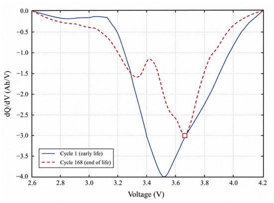
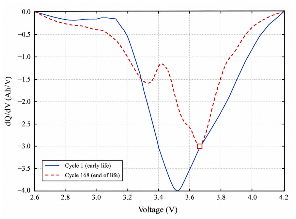
The following are the features obtained of the raw voltage, current, temperature and time series in each discharge cycle. Full derivations are given in the source code that accompanies it. The dQ/dV is calculated on the discharge branch, starting with 35 voltage bins, selected to match the 150 to 250 raw samples that are usually available in one cycle, then a five-point moving average smoothing pass. Two characteristics, |dQ/dV| are recorded. One of the common methods in the literature is charge branch IC analysis; however, the discharge cycles are the ones that bear the label of carrying capacity in this data set; this is recorded in the repository notes. Figure 1 presents the resulting curve and extracted peak of an early-life and an end-of-life cycle of cell B0005 where despite the physical behaviour, the peak flattens with ageing and shifts.
Figure 1.
Incremental capacity (dQ/dV) curve for an early-life and an end-of-life battery.
The remaining features are the start and end voltage of the recorded cycle and the maximum and the rise in temperature. The end-voltage feature is taken as the final recorded voltage sample of the cycle. Because the record continues after the discharge load is removed, that sample is measured once the cell has partly relaxed and is therefore not the discharge cutoff voltage; across the four cells it lies between 0.87 and 1.18 V above the measured cutoff.
All features were examined against ground truth SOH before model training. Within each cell, discharge duration correlates strongly with SOH (r ≈ 0.97), while the internal resistance estimate shows a negative correlation (|r| = 0.64–0.96), consistent with increasing resistance as SOH declines. Under the fixed 2 A constant current protocol, discharged capacity is approximately proportional to time under load, explaining the strong duration SOH correlation. Regressing capacity on time under load yields R2 values of 0.9995–0.99998, with implied currents of 2.015–2.029 A, consistent with the nominal load. The duration feature used in this study represents the full recorded cycle, including the post-load rest interval, and is therefore a noisier proxy for time under load. No windowing is applied during feature extraction; early-cycle windows are imposed subsequently by restricting the discharge cycle rows available for training and evaluation.
5. Modelling Approaches
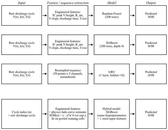
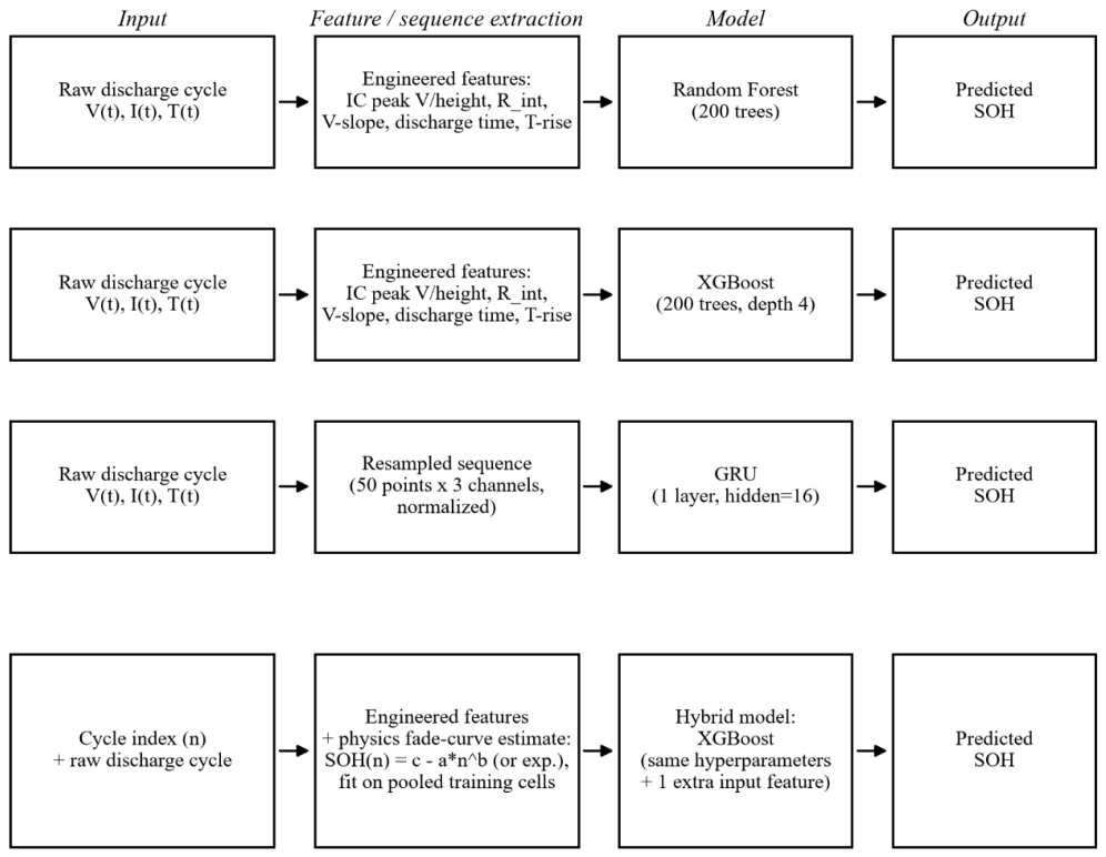
Figure 2 summarises the model architectures compared: Random Forest and XGBoost on engineered per-cycle features, the GRU on resampled raw sequences, and the physics-assisted hybrid, in which the pooled fade curve estimate enters XGBoost as one additional input feature. It is also tested as an independent predictor, the physics fade curve baseline. Evaluation of all models is done at the same leave-one-cell-out protocol at three early-cycle windows W ∈ {20, 50, 100}: a run only transparently observes discharge cycles with cycle index ≤ W, simulating the condition where only the first W cycles of operating history have been recorded.
Figure 2.
Model architectures layout of the proposed system.
Individually, a power law model, SOH(n) = c − a · nb, and an exponential model, SOH(n) = A · exp(−k · n) + C, are each fitted by nonlinear least squares to the pooled (cycle index, SOH) pairs of the three training cells, constrained to cycles not exceeding W. The functional form with the lowest training RMSE is retained. The trained model is then used on the held-out test cell with only cycle index and no per-cell calibration data of the test cell. The zero-shot, population fit physics model is thus a natural baseline, which can be directly compared to the leave-one-cell-out setup of the machine learning models instead of an optimistic per-cell fit.
On the engineered per-cycle features of the three cells used in training, a Random Forest regressor (200 trees, maximum depth 6) and an XGBoost regressor (200 trees, maximum depth 4, learning rate 0.1) are trained on the engineered per-cycle features of the three training cells and tested on the held-out cell. Instead of tuning hyperparameters per-fold, hyperparameters are fixed a priori, which allows for the leave-one-cell-out comparison to be test set-adjacent tuning-free. The model configurations and hyperparameters used for all five approaches, including the physics-assisted hybrid and GRU sequence model, are summarised in Table 2.
Table 2.
Hyperparameters and configuration of every model.
The projected SOH of the physics baseline, calculated without any idea of the test cell is provided as one more input feature to an XGBoost model with the hyperparameters, trained and tested in the same way.
Each discharge cycle voltage, current and temperature series is resampled to 50 on a normalised time axis [0,1], resulting in constant-length inputs despite varying raw sample counts and lengths across cycles, and z-score normalised with training fold statistics. The resampled sequences are sent to a single-layer GRU (hidden size 16) and a linear output layer, which are trained separately in all combinations of window and fold with Adam (learning rate 0.01, 150 epochs, mean squared error loss).
6. Results and Discussions
6.1. Accuracy Across Models and Early-Cycle Windows
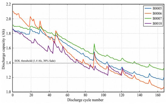
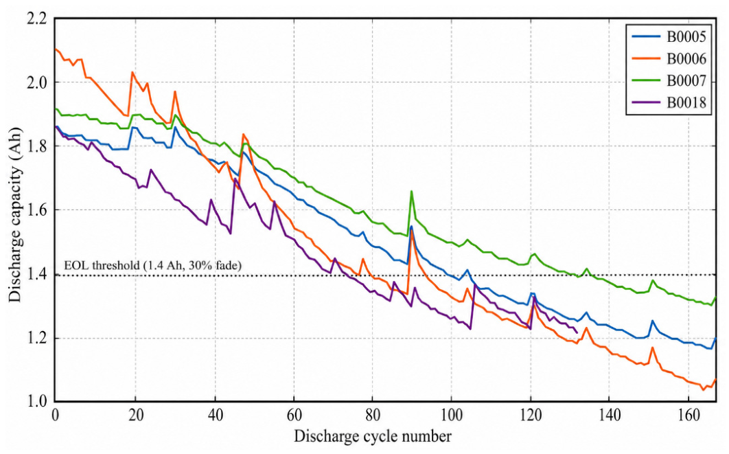
Each model and window uses its pooled predictions, combining all four leave-one-cell-out folds, to compute RMSE, mean absolute error (MAE) and the coefficient of determination (R2), as shown in Table 3. The mean training and inference time per fold is also reported to describe computational cost. RMSE and MAE are treated as the primary metrics. R2 is reported as a supplementary measure and is not comparable across windows, because the variance of the test targets against which it is normalised grows with the window length; Section 6.3 quantifies this effect and reports an evaluation on a common SOH support. Paired Wilcoxon signed rank tests were applied to per-cell RMSE differences between model pairs at each window. With only four cells (n = 4), the smallest attainable two-sided p-value is 0.125; therefore, no comparison reaches conventional significance thresholds. The reported RMSE and R2 rankings should consequently be interpreted as descriptive evidence rather than statistically conclusive differences. Figure 3 shows the capacity fade curves of the four cells against discharge cycle number, together with the end-of-life threshold. The observed non-monotonic capacity recovery excursions are consistent with previously reported relaxation effects in this dataset, associated with rest periods between cycling blocks rather than measurement noise.
Table 3.
Pooled performance and computational cost of every model at each early-cycle window, aggregated over the four leave-one-cell-out folds.
Figure 3.
Discharge capacity fade curves for cells B0005, B0006, B0007 and B0018 (data: NASA PCoE Battery Data Set [14]).
The non-monotonic excursions correspond to the capacity recovery relaxation effect associated with rest periods between cycling blocks.
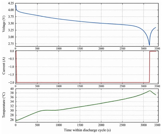
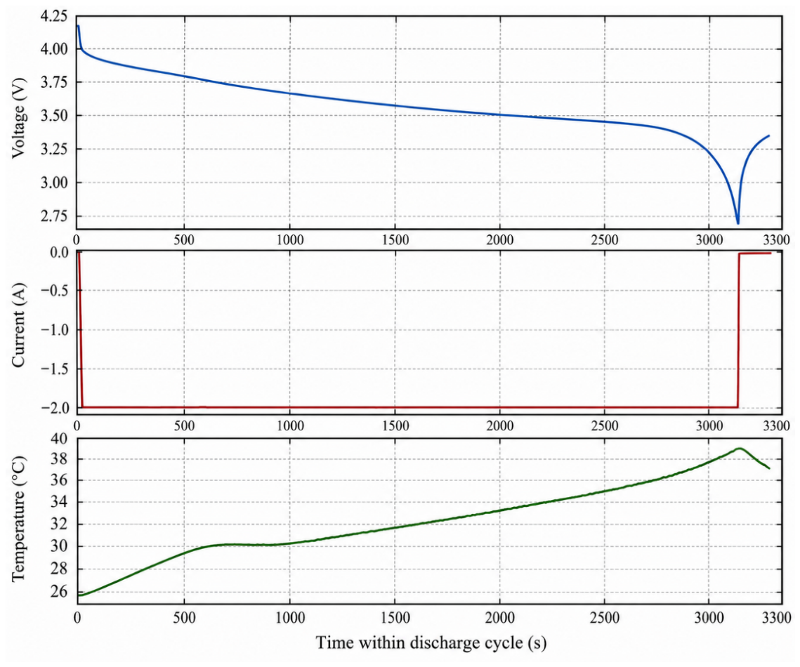
One such single-cycle profile is presented in Figure 4, where terminal voltage, load current and cell surface temperature are plotted versus time during one discharge cycle of cell B0005. The profile validates a constant current discharge shape as hypothesised in all the feature extraction.
Figure 4.
Single-cycle voltage, current and temperature profile (cell B0005, cycle 50).
The incremental capacity feature alone was plotted which compared the dQ/dV curve of an early-life cycle with that of an end-of-life cycle of the same cell. The fact that the extracted peak has shifted and flattened is evidence of the fact that the feature is responding to an ageing-related change in the shape of the curve, as opposed to noise.
At the 20-cycle window, all models yield negative pooled R2 values, indicating limited predictive performance for unseen cells under leave-one-cell-out evaluation. This suggests that 20 early discharge cycles may provide insufficient information to capture cross-cell variability in degradation behaviour. With only three cells available for training (60 training rows), the limited diversity of degradation trajectories may constrain generalisation. Performance improves as longer early-life windows are considered.
Predictive performance improves for the tree-based models at the 50-cycle window. XGBoost achieves R2 = 0.683 and Random Forest R2 = 0.580, compared with −0.098 for the physics-based baseline. At 100 cycles, XGBoost reaches R2 = 0.887, while the physics-based baseline improves to R2 = 0.658. The tree-based models have a slightly larger pooled RMSE in the 100-cycle window than in the 50-cycle window, rising by around 6% for XGBoost and 13% for Random Forest even though R2 increases. This divergence arises because the longer window spans a broader range of SOH values and therefore a larger target variance against which R2 is normalised; Section 6.3 confirms this attribution by repeating the comparison on a common SOH support. RMSE and MAE are therefore used as the main metrics and R2 as a supplementary one. While plain XGBoost produces the lowest RMSE at both windows, the physics-assisted hybrid does not show any measurable improvement under the conditions evaluated, and Section 6.10 identifies the structural reason for this.
The GRU achieves the lowest predictive performance across all windows, with R2 = 0.140 at 100 cycles. Two factors contribute. The first is the limited number of training sequences available under the four-cell leave-one-cell-out design. The second, examined in Section 6.9, is that the normalised time axis used to resample each cycle removes absolute discharge duration from the GRU input, so the sequence model does not receive the quantity that contributes most to the accuracy of the tree-based models.
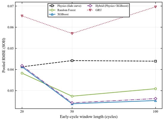
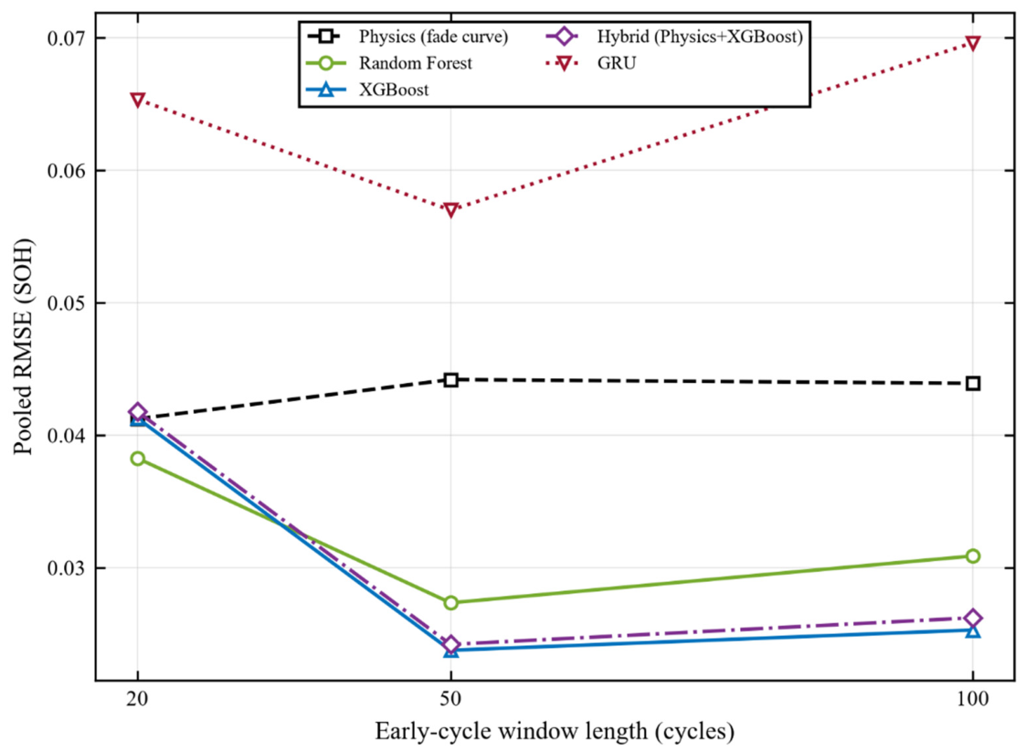
To assess variation across held-out cells, per-fold results are reported alongside pooled metrics. At the 50-cycle window, XGBoost RMSE on the full feature set ranges from 0.0090 for B0005 to 0.0363 for B0006. B0006 is the most difficult held-out cell across all tested windows. Because successive cycles within each cell are correlated, the four cells—not individual cycles—constitute the independent evaluation units, limiting the strength of statistical inference. Figure 5 illustrates the variation in pooled RMSE across early-cycle windows for all five models.
Figure 5.
Pooled RMSE as a function of the early-cycle data window.
6.2. Accuracy as a Function of Available Early-Cycle Data
To examine the effect of window length, the duration-free feature set was evaluated at 20, 30, 40, 50, 60, 80 and 100 cycles using the same leave-one-cell-out protocol and fixed hyperparameters. XGBoost pooled RMSE values were 0.0399, 0.0352, 0.0316, 0.0318, 0.0314, 0.0268 and 0.0319, respectively. Random Forest showed a similar trend, with RMSE decreasing from 0.0413 at 20 cycles to a minimum of 0.0308 at 80 cycles. Typically, errors diminish up to 40 cycles then fluctuate. Across the 40-, 50- and 60-cycle windows, the per-cell RMSE ranged from 0.019 to 0.043, while the difference in pooled RMSE between those three windows was only 0.0004 for XGBoost; across all seven windows, the per-cell range widens to 0.018–0.060.
Both models had the lowest RMSE at 80 cycles and increased RMSE value at 100 cycles. This increase could be due to increased degradation in later cycles, but this has not been confirmed. Direct comparisons should be made with caution as different cycle sets may be evaluated in different windows. The XGBoost RMSE rose around 19% between 80 and 100 cycles, and the R2 value is almost the same (0.818 and 0.819, respectively).
The results describe the association between data availability at early cycles and prediction error and do not provide a minimum cycle threshold. Errors tend to go down as early life history length increases under the evaluated protocol, but with a non-monotonic trend that does not provide a specific “too little is too much” rule.
6.3. Evaluation on a Common SOH Support
Because each early-cycle window spans a different range of SOH values, the coefficient of determination is normalised by a different target variance at each window. Across the four held-out cells, the standard deviation of the test targets rises from 0.0338 SOH units at the 20-cycle window to 0.0751 at the 100-cycle window, so the variance against which R2 is computed increases by a factor of 4.9. An evaluation in which every window is scored on the same SOH range therefore separates the effect of additional training data from the effect of a changing test distribution.
A single SOH interval shared by all four cells at all windows does not exist in this dataset. At the 20-cycle window the intersection of the four cells’ SOH ranges is empty, the lower bound of 0.9338 set by B0006 exceeding the upper bounds of 0.9282 and 0.9275 set by B0005 and B0018; B0006 begins above the rated capacity, with a first-cycle SOH of 1.0177. A per-cell construction is used instead. Within a cell the SOH range at a given window is contained in its range at any longer window, because the maximum is fixed by the first cycle and the minimum falls as the window grows, so the intersection across all windows is exactly that cell’s range at the shortest window evaluated. Restricting the evaluation rows of every window to that band gives each cell an identical test support at all windows while the training window continues to grow. The bands are therefore determined by the data rather than selected. From the 40-cycle window onwards, the evaluation set is identical at every window and comprises 118 observations, against 80 at the 20-cycle window and 108 at the 30-cycle window.
Table 4 reports the comparison. Under the common support the pooled RMSE of XGBoost improves from 0.0413 at the 20-cycle window to 0.0243 at the 50-cycle window and then varies within approximately 0.006 without further systematic improvement, which reproduces and confirms the plateau identified in Section 6.2. The behaviour of R2 is different: under the unrestricted evaluation it rises from −0.488 to 0.887, whereas under the common support it reaches 0.368 at the 50-cycle window and does not increase thereafter, ending at 0.021 at the 100-cycle window. The physics baseline shows the same pattern more starkly, its unrestricted R2 rising to 0.658 at the 100-cycle window while its common support value remains between −0.63 and −0.79 at every window. The improvement in R2 with observation window length reported under the unrestricted evaluation is therefore attributable to the widening distribution of test targets rather than to improved estimation. The ranking of the model families is largely unaffected, changing at two of the seven windows and in both cases between models separated by less than 0.002 RMSE. This analysis provides a more controlled basis for interpreting observation window effects than the unrestricted comparison alone.
Table 4.
Pooled RMSE (SOH units) and R2 for XGBoost, and physics baseline.
6.4. Early-Window Estimation Versus Future Cycle Forecasting
The protocol defined in Section 3 draws both the training and the evaluation observations from cycles 1 to W, so the quantity estimated is contemporaneous with the measurements rather than ahead of them. Predicting future SOH from early-life measurements is a distinct task, and a complementary temporal evaluation was carried out to quantify the difference. Two additional protocols were defined alongside the primary one. In the first, the models are trained on cycles 1 to W of the three training cells and evaluated on cycles beyond W of the held-out cell. In the second, the held-out cell’s own cycles 1 to W are added to the training set, which reflects the situation of a battery management system that holds its own cell’s early history. In both cases the split is strictly temporal and no observation beyond cycle W enters training, a condition verified by automated checks on every fold.
Table 5 reports the outcome for XGBoost on the full feature set. Forecasting later-life SOH is between 1.9 and 4.3 times less accurate in RMSE than estimating SOH within the observed window, and every machine learning model returns a negative pooled R2 at every window under both temporal protocols. Supplying the held-out cell’s own early history reduces the error by 6 to 17 percent at windows of 40 cycles and above. The ordering of the model families also differs between the two tasks: the physics baseline, which is the least accurate model for in-window estimation at every window, is the most accurate of those evaluated at the 40-cycle window under the temporal protocol, reaching a pooled RMSE of 0.0396 against 0.0967 for XGBoost, while at the 80-cycle window its error rises to 0.1475 and it becomes the least accurate. A parametric fade curve extrapolates beyond the fitted range, whereas a tree ensemble predicts within the range of target values present in its training data and so cannot follow a trajectory into more degraded states; the instability of the fade curve at longer windows reflects the selection of its functional form on in-window training error alone, without a criterion for extrapolation behaviour.
Table 5.
Pooled RMSE (SOH units) for XGBoost on the full feature set under the primary in-window protocol (A) and under two temporal protocols, with window in discharge cycles.
This evaluation is reported as a complementary analysis and does not replace the primary protocol for which the study was designed. Its value is in establishing that results obtained for cross-cell estimation within an early-life window should not be read as evidence of forecasting capability, and that the relative standing of physics-based and data-driven models depends on which of the two tasks is being performed. Neither model family is reliable for forecasting at the present sample size.
6.5. Prediction and Residual Behaviour
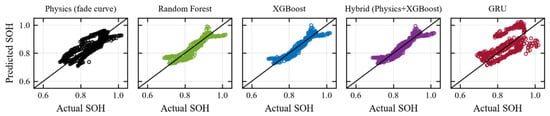
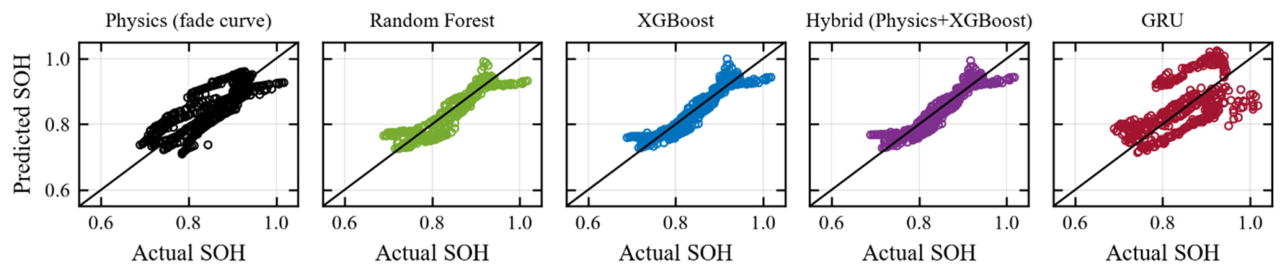
Figure 6 presents the predicted versus actual SOH scatter plot of all the five models at the 100-cycle window, pooled across the four leave-one-cell-out folds. The physics baseline has an artificially high SOH over-fitting to the more heavily degraded cells, which can be explained by the fact that it is not a per-cell fit but a population-level curve. XGBoost, Random Forest and the hybrid model follow the diagonal in the mid-SOH range but flatten a bit at the largest observed SOH values, a regression-towards-the-mean effect at the edges of the training distribution. GRU predictions are graphically more dispersed and more biased.
Figure 6.
Predicted versus actual SOH for all five models.
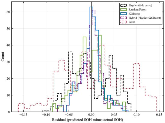
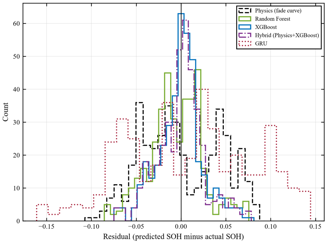
Figure 7 presents the distributions of residual error, consistent with the other views: residuals are tighter and more symmetric for XGBoost, Random Forest and the hybrid model, and wider and more biased for the physics baseline and GRU.
Figure 7.
Distribution of residual errors for all five models at the 100-cycle window.
6.6. Feature Importance and the Discharge Duration Ablation
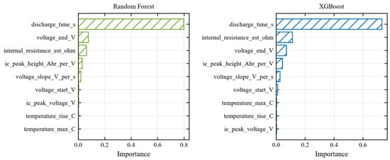
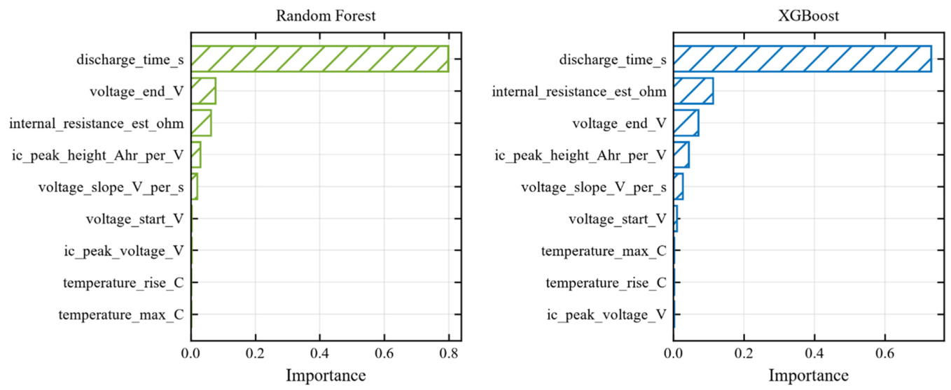
Figure 8 presents the mean feature importance of the Random Forest and XGBoost models, averaged over the four leave-one-cell-out folds of the 100-cycle window. Discharge duration is the most important feature in both models, with a score of about 0.80 in Random Forest and 0.73 in XGBoost, exceeding internal resistance, end-of-discharge voltage and the incremental capacity features.
Figure 8.
Mean feature importance for Random Forest and XGBoost.
Under the constant current discharge to a fixed cutoff voltage used in this dataset, the charge removed is approximately the product of current and time under load, so discharge duration is closely related to the capacity from which the SOH target is derived: a less degraded cell takes longer to reach the same cutoff voltage at the same current. The duration feature actually used is the full recorded cycle length rather than the time under load, and is therefore a noisier form of that quantity, but the dependence remains. The high accuracy of the tree-based models is thus obtained on a task in which one feature is close to a capacity readout, and the ablation reported below quantifies how much of that accuracy the feature accounts for.
Four information-matched configurations were therefore compared at each window: a cycle index-only baseline, a duration-only baseline, the full engineered feature set, and the full set with the duration feature removed. Folds, hyperparameters and all other settings were held identical across the four.
Removing discharge duration raises pooled XGBoost RMSE from 0.0238 to 0.0318 at the 50-cycle window, an increase of 34%, and from 0.0253 to 0.0319 at 100 cycles, an increase of 26%. The comparative result nevertheless holds: the duration-free model reaches R2 = 0.431 at 50 cycles against the physics baseline at R2 = −0.098, and R2 = 0.819 at 100 cycles against 0.658. At both windows the duration-only baseline and the full-minus-duration model give the same pooled RMSE to four decimal places, 0.0318 and 0.0319 respectively, so this one feature carries about as much information on its own as the eight remaining engineered features do on theirs. Since the full nine-feature set is substantially better than either subset, the two groups carry partly complementary information, and the voltage-, resistance- and incremental capacity-based indicators contribute a real independent signal rather than a redundant one.
A further configuration bounds the protocol effect from above. Replacing the full-record duration with the time under load alone, computed from the current trace, gives a pooled RMSE of 0.0196 at 50 cycles and 0.0144 at 100 cycles from that single feature, better than the full nine-feature set at either window. This confirms that the accuracy attainable on this dataset is governed largely by the near-deterministic Coulomb-counting relationship created by the constant current protocol, and not by model capacity. The full-record duration feature was retained in the reported models rather than being replaced by the time under load, so that the configuration evaluated here matches the one described in Section 4, and Section 6.11 examines whether the dependence persists under variable-current loading; the time-under-load result is reported as a diagnostic of the protocol, not as a proposed estimator.
6.7. Influence of Per-Cell Discharge Cutoff Voltage
The four cells are discharged to different cutoff voltages, and the effect of this heterogeneity on the leave-one-cell-out evaluation was examined directly. The cutoff actually reached on each cycle was measured as the lowest voltage recorded while the discharge load was applied. Table 6 reports the result alongside the nominal values stated in the dataset documentation. The measured cutoffs are between 0.04 and 0.10 V below nominal, a consequence of the approximately 18 s sampling interval, and B0007 discharges to between 0.31 and 0.56 V below the other three cells. Consistent with this, B0007 has the longest median time under load and is the only cell that does not reach the 30 percent fade criterion within its recorded life.
Table 6.
Nominal and measured discharge cutoff voltage.
The measurement also clarifies the end-voltage feature introduced in Section 4. Because each record continues after the load is removed, the final recorded voltage is measured after partial relaxation and lies between 0.87 and 1.18 V above the measured cutoff. The length of the recorded rest interval differs substantially between cells, with median values of 311 s for B0005, 395 s for B0006, 118 s for B0007 and 271 s for B0018, so the differences between cells in this feature reflect both the cutoff voltage and the logging schedule. The feature nevertheless carries a clear degradation signal, correlating with SOH within each cell at between −0.74 and −0.96.
Cutoff heterogeneity propagates into the evaluation through four routes. A lower cutoff extracts more charge, so for a given degradation state, B0007 records a higher capacity and, against the fixed 2.0 A·h denominator, a higher SOH. A lower cutoff also lengthens the time under load, so the duration-to-SOH relationship learned from three cells is systematically offset when applied to a cell discharged to a different cutoff. The end-voltage feature is affected as described above. Finally, the incremental capacity features are binned over the observed voltage range of each cycle, so a wider range is divided into the same number of bins at coarser resolution.
A sensitivity analysis was carried out in which B0007 was excluded and the leave-one-cell-out evaluation repeated over the remaining three cells with identical models, hyperparameters and random seed. Pooled RMSE generally increases rather than decreases, by up to a factor of 1.46 for XGBoost at the 50-cycle window, and the ordering of the model families changes at the 20-, 40- and 50-cycle windows while remaining unchanged at the 80- and 100-cycle windows. This comparison changes two conditions simultaneously, since removing a cell also reduces each training fold from three cells to two, and the two effects cannot be separated at this sample size. The analysis therefore does not establish that cutoff variation is without effect; what it does show is that the ordering of closely spaced models at short windows is sensitive to the composition of a four-cell panel, which is a concrete demonstration of the statistical limitation noted in Section 6.1.
6.8. Sensitivity to Modelling and Feature Extraction Settings
Robustness was assessed using nested leave-one-cell-out cross-validation, with hyperparameters selected through an inner search over a predefined grid using only the three training cells. The resulting error, which is not informed by the held-out cell, is 0.0365 for Random Forest and 0.0317 for XGBoost at the 50-cycle window, and 0.0309 and 0.0275 at the 80-cycle window. These values lie within 0.0008 RMSE of the fixed configurations used throughout; the nested procedure is marginally better in two of the four cases and marginally worse in the other two, which indicates that the fixed configurations were not favourably tuned. Across the whole predeclared grid the total spread in pooled RMSE is 0.0016 to 0.0046 depending on window and model, against pooled RMSE values of approximately 0.03; the number of trees contributes a marginal effect of at most 0.0004, and maximum depth is the only parameter with an appreciable influence. No configuration was selected using held-out-cell performance.
Sensitivity to incremental capacity extraction settings was assessed across nine combinations of voltage bin counts and smoothing widths. Across these settings, the total spread in pooled RMSE is 0.0023 to 0.0050, again against pooled RMSE values of approximately 0.03, with the selected configuration ranking third to fifth of nine depending on the model and window. Although peak voltage extraction varies substantially (r = −0.33 for 20 bins and seven-point smoothing relative to the baseline), the resulting pooled RMSE remains within this range. These results suggest that the main conclusions are relatively insensitive to the extraction settings, although the extracted features themselves are sensitive to parameter selection.
6.9. Input Representation and the Sequence Model Comparison
The sequence model receives each discharge cycle resampled to 50 points on a time axis normalised to the unit interval, as described in Section 5. Normalising the time axis divides out the absolute length of the cycle, so the GRU does not receive discharge duration, which Section 6.6 identifies as the most influential feature for the tree-based models. The comparison reported in Table 3 is therefore not matched in the information available to each model family, and an additional evaluation was carried out to quantify the consequence.
Four input configurations were compared, holding the folds, the cycles evaluated, the random seed, the hidden size, the optimiser, the learning rate, the number of epochs and the loss function identical to the configuration in Table 2. The first reproduces the published input representation. The second supplies absolute discharge duration as an additional scalar. The third supplies discharge duration together with cycle index. The fourth supplies absolute elapsed time as a fourth sequence channel. Scalar inputs are standardised using training fold statistics only, and no configuration was selected on the basis of held-out performance. Table 7 reports the pooled results.
Table 7.
Pooled RMSE (SOH units) of the GRU under four input configurations.
Restoring the discarded information improves the sequence model substantially at the longer windows. Supplying discharge duration reduces pooled RMSE by 16 percent at the 50-cycle window and 34 percent at the 100-cycle window, and supplying duration together with cycle index reduces it by 23 and 45 percent, respectively, raising R2 at the 100-cycle window from 0.143 to 0.738. Measured against the gap to XGBoost on the same observations, the best configuration closes 38 percent of that gap at the 50-cycle window and 70 percent at the 100-cycle window. At the 20-cycle window, the additional inputs instead increase the error, by between 18 and 23 percent, which is consistent with the limited number of training sequences available at that window. The GRU remains less accurate than XGBoost at every window, so the ranking reported in Table 3 is unchanged; what the analysis establishes is that a substantial part of the difference originates in the input representation rather than in the model architecture or the sample size alone, and the discussion in Section 6.15 is framed accordingly.
These additional configurations were evaluated in a software environment whose deep learning library version differs from the one used for Table 3. The reproduced baseline matches the published values at the 20- and 100-cycle windows to within 0.001 RMSE and differs by 0.005 at the 50-cycle window. All four configurations in Table 7 were evaluated in the same environment, so the comparison between them is internally consistent.
6.10. Physics-Assisted Feature Integration in a Tree Ensemble
The physics-assisted hybrid supplies the fade curve estimate to XGBoost as one additional input feature. The fade curve is fitted on the pooled cycle index and SOH pairs of the three training cells within the window and applied to the held-out cell using cycle index alone, so no information from the held-out cell enters the fit. Both candidate functional forms are strictly decreasing in cycle index, which means that the appended feature is a strictly monotonic transformation of cycle index and carries no per-cell measurement. Across the folds its correlation with cycle index lies between −0.995 and −0.998.
A gradient-boosted tree ensemble partitions each feature at thresholds and is therefore invariant to any strictly monotonic transformation of an individual feature: the induced partition, and hence the fitted model, is unchanged. Appending a fade curve estimate to such an ensemble consequently cannot provide information beyond the ordering already carried by cycle index, whatever the quality of the fade curve. Table 8 demonstrates this directly. Appending the fade curve estimate and appending cycle index give identical pooled RMSE to five decimal places at every window. An oracle configuration, in which the fade curve is fitted on the held-out cell’s own data and which is reported solely as a theoretical upper bound because it uses information that would not be available in practice, gives the same values again, although the two feature vectors differ numerically by up to 0.047 SOH units.
Table 8.
Pooled RMSE (SOH units) of XGBoost with the nine engineered features.
The representativeness of the fade curve was examined separately. A single population curve fitted to all four cells has an in-sample RMSE two to four times larger than curves fitted to each cell individually, with a per-cell bias of up to 0.046 SOH units, so the pooled curve does not describe the individual trajectories closely. This supports the view that the empirical fade model is a coarse description of cell-specific degradation, but the equivalence result shows that improving it would not alter the hybrid’s predictions. The limitation applies to the specific strategy of appending a scalar physics estimate to a tree ensemble, and not to physics-informed approaches in general. Couplings that are not monotonic functions of cycle index, such as predicting the residual from a physics model rather than supplying its output as an input feature, constraining the loss function, or using physics-derived quantities that vary within a discharge cycle, are not subject to this equivalence and remain open directions.
6.11. Companion Evaluation Under Variable-Current Loading
The NASA Randomized Battery Usage Data Set, Part 2 [44,45] was used to evaluate four 18650 cells (RW3-RW6) cycled at room temperature between 4.2 V and 3.2 V with discharge currents drawn randomly between 0.5 and 4 A. Reference charge and discharge cycles performed after every 50 random walk cycles provide the capacity ground truth, each checkpoint containing two replicate reference discharges that are averaged before SOH is formed. Because the dataset documentation states no rated capacity for these cells, SOH is defined relative to each cell’s own first reference capacity rather than to a nominal rating. The first barrier is excluded as a target because no random walk history precedes it, leaving 69 targets. For a target at checkpoint k, model inputs are drawn only from random walk activity recorded before that checkpoint; all characterisation steps, including reference charge and discharge, pulsed load and low-current steps, are excluded wherever they occur, and imputation statistics are fitted on training cells only within each fold.
The relationship between discharge duration and capacity weakens under variable loading, with R2 values of 0.700–0.814, compared with 0.9995–0.99998 under constant current loading. Residual standard deviation increases to 0.205–0.212 Ah, a 60–250-fold increase over the constant current results.
Using 69 leave-one-cell-out reference checkpoint targets, the combined usage history and present-state model achieves a pooled RMSE of 0.0281 SOH units, compared with 0.1159 for the training fold mean baseline. Duration-only and usage history-only models achieve RMSE values of 0.0378 and 0.0402, respectively, while removing both feature groups increases RMSE to 0.0777. At the widest window, duration is the most important individual feature (0.4153), although usage history features collectively account for 0.4962. At a narrower window, duration importance falls to 0.1110, while usage history features account for 0.7671. Thus, duration remains informative under variable loading, but its predictive contribution depends on the observation window.
The companion variable-current evaluation extends the investigation to four additional NASA cells, with reference checkpoints representing successive stages of cell ageing. These checkpoints are treated as sequential observations rather than independent replicates. The analysis differs from the main study in its SOH reference (initial reference capacity rather than rated capacity), feature set (incremental capacity features are excluded because random walk voltage profiles are non-monotonic), and evaluation unit (checkpoints summarising 50 cycles). Therefore, it provides complementary evidence on measurement protocol dependence, rather than directly comparable results or independent external validation under real-world EV driving conditions.
6.12. Computational Cost
Mean per-fold training time was about 0.05 to 0.06 s in the case of physics baseline and 0.09 to 0.16 s in the case of XGBoost and the hybrid model, to 0.31 to 0.43 s in the case of Random Forest and 5.26 to 6.71 s in the case of GRU. Every model had an inference time of at most about 0.02 s per fold, and the physics baseline under 0.5 ms (Table 3). All five methods are cheap at inference when a BMS or fleet analytics application requires retraining model periodically but needs to score new data cheaply and often. The training cost of the GRU is approximately 12 to 61 times that of the tree-based models across the windows evaluated, and 33 to 49 times that of XGBoost specifically. Combined with its lower accuracy in this data regime, this makes it the least attractive option in the present setting, although the result is specific to the small number of cells considered here and would be expected to change with a larger cell population and a longer training budget.
6.13. Remaining Useful Life
A full leave-one-cell-out RUL regressor was not attempted because only three cells (B0005, B0006 and B0018) reach the 30% fade end-of-life criterion within the observed cycle range, providing insufficient independent training cells. Supplementary Analysis (Table S1 and Figure S1) extrapolates the Section 5 fade curve model to the end-of-life threshold, yielding mixed results: errors of six cycles for B0006 and 25 cycles for B0005, while B0018 does not reach the threshold within 400 cycles. These results indicate that early-window physics-based extrapolation is unreliable with the available data; therefore, no RUL prediction claim is made.
6.14. Applicability to Battery Management Systems
Translating these results into an operational battery management system requires several developments, which the present study scopes rather than delivers. The engineered features are defined over a complete discharge cycle: the duration, start and end voltages, voltage slope, temperature statistics and incremental capacity descriptors all presuppose a discharge from a full charge to the cutoff voltage, and the internal resistance proxy additionally requires a rest interval immediately before the load is applied. An electric vehicle discharges from whatever state of charge is present to whatever state of charge the journey ends at, so complete cycles of this kind are rarely available and most of the present features would require redefinition for partial discharge segments. The incremental capacity features are the most sensitive in this respect, since a partial voltage span alters both the binning and the peak that is selected.
Operating conditions impose two further requirements. All cells considered here were cycled at 24 °C, so the study provides no evidence on temperature generalisation, and two of the nine features are absolute temperature quantities that would be evaluated outside their training distribution in a vehicle operating across a wide ambient range. Under variable loading the near-deterministic relationship between discharge duration and capacity does not hold, as Section 6.11 shows, although the companion evaluation also indicates that a feature set built on cumulative usage history retains useful predictive value in that setting, which suggests the appropriate direction for a field-oriented feature design. Training the models additionally requires reference capacity measurements, which are available in a laboratory or from fleet vehicles taken out of service but not from a vehicle in normal use; inference itself requires no such measurement.
Computational cost is not a constraint. As Table 3 shows, inference takes at most approximately 0.02 s per fold for all five models, which corresponds to microseconds per cycle and is well within the capability of battery management hardware, while training is an offline activity performed at fleet level. The estimator is, however, cycle-level and batch-oriented rather than recursive, and produces a point estimate without an associated uncertainty, whereas a deployed system would typically require a continuously updated estimate with a confidence interval. A realistic validation pathway would therefore combine partial discharge feature definitions, data gathered at several temperatures, representative drive cycle loading, and measurements at module and pack level, followed by a recursive formulation with uncertainty quantification. The value of the present study for that pathway lies in identifying which part of the accuracy reported on laboratory benchmarks depends on the measurement protocol, and therefore which part should not be expected to transfer.
6.15. Discussion and Limitations
Tree-based models provide useful SOH estimates from several tens of early discharge cycles. Pooled RMSE shows no consistent improvement beyond approximately 40 cycles, and the common support evaluation in Section 6.3 confirms that this plateau is a property of the estimation task rather than of the evaluation design, while the accompanying rise in R2 is attributable to the widening distribution of test targets. The physics-based baseline is less accurate overall for in-window estimation, and the GRU underperforms the tree-based models for the two reasons identified in Section 6.9. These findings describe a trend rather than a minimum data threshold; larger-scale validation is required before deployment criteria can be established.
Discharge duration is both the most influential feature and an important limitation. Under fixed current discharge to a fixed cutoff voltage, duration is closely related to discharged capacity and therefore to the SOH target. Excluding duration increases RMSE by 34% at 50 cycles and 26% at 100 cycles, while preserving the model ranking. Consequently, the reported XGBoost RMSE of 0.025 SOH units at 100 cycles should not be assumed to transfer to field conditions with variable loads. The companion evaluation indicates that duration dependence weakens under randomised loading but persists.
The physics-assisted hybrid does not improve upon plain XGBoost. The equivalence analysis in Section 6.10 shows that this outcome is structural: a gradient-boosted tree ensemble is invariant to strictly monotonic transformations of an individual feature, and the fade curve estimate is a strictly monotonic function of cycle index, so appending it cannot create partition information that cycle index would not already provide. The term physics-assisted is therefore appropriate: the model incorporates a physics-motivated input but does not impose physical constraints on its architecture or loss function. This finding concerns the specific strategy of appending a scalar physics estimate to a tree ensemble and should not be read as a general statement about physics-informed methods, which include formulations that constrain the model structure or the loss function directly.
The scope of the present investigation is defined by several factors. The primary evaluation uses four cells of one chemistry at 24 °C, which bounds statistical inference and generalisability; the leave-one-cell-out design makes the fullest use of this population by evaluating every cell as an unseen cell in turn. Extending the evaluation to further cells of the same dataset was considered. The BatteryAgingARC-FY08Q4 subset used here comprises exactly these four cells, and published descriptions of the remaining groups of the NASA PCoE Battery Data Set indicate different discharge current levels, and in one group a second ambient temperature, so incorporating them would alter the operating conditions that the controlled design holds fixed rather than enlarge the sample under matched conditions. No additional cells were therefore included. Independent external validation on a separate cell population has not been performed, and the companion evaluation of Section 6.11, which uses four additional cells under a different loading protocol, is complementary evidence on protocol dependence rather than external validation of the main results. The dependence of the engineered features on the constant current discharge protocol bounds the transferability of the absolute error values, as Section 6.6 and Section 6.11 quantify. Different cycle sets are evaluated across windows in the unrestricted comparison, which Section 6.3 addresses through the common support evaluation. The GRU uses a deliberately compact, CPU-trainable architecture, and larger or pretrained sequence models may behave differently. RUL prediction remains outside the validated scope of this study and is limited to the illustrative Supplementary Analysis. Section 6.14 sets out the further development required before the framework could be applied in an operational battery management system.
7. Conclusions
This study built a reproducible pipeline, running from raw and unmodified NASA PCoE.mat files through feature engineering and five model families to a controlled leave-one-cell-out evaluation, in order to establish how much of the accuracy reported for early-life SOH estimation is attributable to the measurement protocol rather than to the estimator. On this four-cell dataset, tree-based machine learning, and XGBoost in particular, outperforms a population fit physics baseline for cross-cell estimation within an observed early-life window once several tens of early cycles are available. Estimation error falls as early-cycle history accumulates up to approximately 40 cycles and changes little thereafter, a plateau that is confirmed when every window is evaluated on a common SOH support; the accompanying improvement in R2 is shown to reflect the widening distribution of test targets rather than improved estimation. The available four-cell dataset and tested windows do not establish a definitive minimum data threshold. Discharge duration is the dominant feature under the fixed-current protocol of this dataset: removing it raises pooled RMSE by 26% to 34% while preserving the ranking of the model families, and a single time-under-load feature outperforms the full nine-feature set, which locates a substantial part of the attainable accuracy in the measurement protocol rather than in model capacity. The compact GRU showed lower predictive performance than the tree-based models, in part because the normalised time axis removes absolute discharge duration from its input; restoring that information reduces its error substantially without closing the gap. A complementary temporal evaluation shows that predicting future SOH from early-life data is a measurably harder task than estimating SOH within the observed window. A companion evaluation under randomised variable current loading indicates that the duration dependence weakens substantially without disappearing. The study is limited to four cells of one chemistry at one temperature and does not include independent external validation, so the absolute accuracy values reported here should be treated as specific to this dataset and protocol.
Supplementary Materials
The following supporting information can be downloaded at: https://www.mdpi.com/article/10.3390/wevj17110613/s1, Section S1: Illustrative remaining-useful-life analysis; Section S2: Data and code provenance; Table S1: Early-window physics extrapolation of the end-of-life cycle; Figure S1: Physics fade-curve extrapolation.
Author Contributions
Conceptualization, methodology, investigation, formal analysis, writing—original draft preparation, and supervision, G.A.; validation, resources, data curation, software, writing—review and editing, and visualization, U.S., S.J. and S.R.S. All authors have read and agreed to the published version of the manuscript.
Funding
Woosong University’s Academic Research Funding—2026.
Data Availability Statement
All results in the main text were obtained from the Li-ion Battery Aging Data Set of the NASA Ames Prognostics Center of Excellence (PCoE), specifically the BatteryAgingARC files for cells B0005, B0006, B0007 and B0018. The companion variable current evaluation in Section 6.11 used the NASA Randomized Battery Usage Data Set, Part 2 (uniform distribution discharge, room temperature), comprising cells RW3, RW4, RW5 and RW6. Both datasets are openly available from the NASA Prognostics Data Repository and were used without modification; no new experimental data were generated in this study. The analysis code, the preprocessing and quality control decisions, the engineered feature definitions and the scripts that regenerate every table and figure reported here and in the Supplementary Materials are available from the corresponding author on reasonable request.
Conflicts of Interest
The authors declare no conflicts of interest.
References
- Waseem, M.; Lakshmi, G.S.; Amir, M.; Ahmad, M.; Suhaib, M. Advancement in Battery Health Monitoring Methods for Electric Vehicles: Battery Modelling, State Estimation, and Internet-of-Things Based Methods. J. Power Sources 2025, 633, 236414. [Google Scholar] [CrossRef] [Scilit]
- Li, M.; Xu, W.; Zhang, S.; Liu, L.; Hussain, A.; Hu, E.; Zhang, J.; Mao, Z.; Chen, Z. State of Health Estimation and Battery Management: A Review of Health Indicators, Models and Machine Learning. Materials 2025, 18, 145. [Google Scholar] [CrossRef] [Scilit] [PubMed]
- Pradhan, S.K.; Chakraborty, B. Battery Management Strategies: An Essential Review for Battery State of Health Monitoring Techniques. J. Energy Storage 2022, 51, 104427. [Google Scholar] [CrossRef] [Scilit]
- Su, L.; Xu, Y.; Dong, Z. State-of-Health Estimation of Lithium-Ion Batteries: A Comprehensive Literature Review from Cell to Pack Levels. Energy Convers. Econ. 2024, 5, 224–242. [Google Scholar] [CrossRef] [Scilit]
- Zhang, Q.; Rong, H.; Zhao, D.; Pei, M.; Dong, X. A Critical Review of the State Estimation Methods of Power Batteries for Electric Vehicles. Energies 2025, 18, 3834. [Google Scholar] [CrossRef] [Scilit]
- Nagulapati, V.M.; Lee, H.; Jung, D.; Brigljevic, B.; Choi, Y.; Lim, H. Capacity Estimation of Batteries: Influence of Training Dataset Size and Diversity on Data Driven Prognostic Models. Reliab. Eng. Syst. Saf. 2021, 216, 108048. [Google Scholar] [CrossRef] [Scilit]
- Roman, D.; Saxena, S.; Robu, V.; Pecht, M.; Flynn, D. Machine Learning Pipeline for Battery State-of-Health Estimation. Nat. Mach. Intell. 2021, 3, 447–456. [Google Scholar] [CrossRef] [Scilit]
- Rout, S.; Samal, S.K.; Gelmecha, D.J.; Mishra, S. Estimation of State of Health for Lithium-Ion Batteries Using Advanced Data-Driven Techniques. Sci. Rep. 2025, 15, 30438. [Google Scholar] [CrossRef] [Scilit] [PubMed]
- Severson, K.A.; Attia, P.M.; Jin, N.; Perkins, N.; Jiang, B.; Yang, Z.; Chen, M.H.; Aykol, M.; Herring, P.K.; Fraggedakis, D.; et al. Data-Driven Prediction of Battery Cycle Life before Capacity Degradation. Nat. Energy 2019, 4, 383–391. [Google Scholar] [CrossRef] [Scilit]
- Deng, Y.; Du, C.; Ren, Z. A Novel Method for Estimating the State of Health of Lithium-Ion Batteries Based on Physics-Informed Neural Network. Batteries 2025, 11, 49. [Google Scholar] [CrossRef] [Scilit]
- Navidi, S.; Thelen, A.; Li, T.; Hu, C. Physics-Informed Machine Learning for Battery Degradation Diagnostics: A Comparison of State-of-the-Art Methods. Energy Storage Mater. 2024, 68, 103343. [Google Scholar] [CrossRef] [Scilit]
- Salem, N.M.; Mohamed, A. Physics-Informed Hybrid Reinforcement Learning for Estimating Lithium-Ion Battery State of Health. Sci. Rep. 2025, 15, 43819. [Google Scholar] [CrossRef] [Scilit] [PubMed]
- Eltamaly, A.M.; Almutairi, Z. Hybrid Physics-Informed Machine Learning Framework for Calibration-Free Degradation Prediction of Lithium-Ion Batteries. Sci. Rep. 2026, 16, 26217. [Google Scholar] [CrossRef] [Scilit] [PubMed]
- Saha, B.; Goebel, K. Battery Data Set; NASA Prognostics Data Repository, NASA Ames Research Center: Moffett Field, CA, USA, 2007. Available online: https://phm-datasets.s3.amazonaws.com/NASA/5.+Battery+Data+Set.zip (accessed on 17 November 2026).
- Liu, X.; Yang, C.; Meng, Y.; Zhu, J.; Duan, Y. Capacity Estimation of Li-Ion Battery Based on Transformer-Adversarial Discriminative Domain Adaptation. AIP Adv. 2023, 13, 075113. [Google Scholar] [CrossRef] [Scilit]
- Modekwe, G.; Al-Wahaibi, S.; Lu, Q. Transformer-Based Capacity Prediction for Lithium-Ion Batteries with Data Augmentation. IFAC-PapersOnLine 2024, 58, 408–413. [Google Scholar] [CrossRef] [Scilit]
- Wang, G.; Lyu, Z.; Li, X. An Optimized Random Forest Regression Model for Li-Ion Battery Prognostics and Health Management. Batteries 2023, 9, 332. [Google Scholar] [CrossRef] [Scilit]
- Hu, J.; Chang, J.; Zhang, Z.; Wang, C.; Jian, X.; Wang, J.; Liu, Q. A Hybrid XGBoost-Augmented Gaussian Process Framework for Accurate Battery State-of-Health Estimation. J. Electrochem. Soc. 2026, 173, 050510. [Google Scholar] [CrossRef] [Scilit]
- Liu, X. Comparative Machine Learning Approaches for Battery Capacity Prediction Using Random Forest and LSBoost Regression Algorithms. J. Electrochem. Soc. 2026, 173, 050511. [Google Scholar] [CrossRef] [Scilit]
- Khan, W.; Aziz, A.; Yousaf, M.Z.; Renhai, F.; Mao, Y.; Latif, M.W.; Tonghao, W.; Khan, B.; Mabunda, N.E.; Ali, A. Hybrid XGBoost-LSTM Model for State-of-Health Prediction of Lithium-Ion Batteries under Different Thermal Conditions. Int. J. Electrochem. Sci. 2026, 21, 101218. [Google Scholar] [CrossRef] [Scilit]
- Chen, Y.; Meng, J.; Ming, S.; Tong, G.; Qi, Z. Improved Deep Extreme Learning Machine for State of Health Estimation of Lithium-Ion Battery. Int. J. Energy Res. 2024, 2024, 8892634. [Google Scholar] [CrossRef] [Scilit]
- Iftikhar, M.; Shoaib, M.; Altaf, A.; Iqbal, F.; Villar, S.G.; Dzul Lopez, L.A.; Ashraf, I. A Deep Learning Approach to Optimize Remaining Useful Life Prediction for Li-Ion Batteries. Sci. Rep. 2024, 14, 25838. [Google Scholar] [CrossRef] [Scilit] [PubMed]
- Chen, C.; Wei, J.; Li, Z. Remaining Useful Life Prediction for Lithium-Ion Batteries Based on a Hybrid Deep Learning Model. Processes 2023, 11, 2333. [Google Scholar] [CrossRef] [Scilit]
- Song, B.; Yue, G.; Guo, D.; Wu, H.; Sun, Y.; Li, Y.; Zhou, B. Prediction of the Remaining Useful Life of Lithium-Ion Batteries Based on Mode Decomposition and ED-LSTM. Batteries 2025, 11, 86. [Google Scholar] [CrossRef] [Scilit]
- Fan, Y.; Lin, Z.; Wang, F.; Zhang, J. A Hybrid Approach for Lithium-Ion Battery Remaining Useful Life Prediction Using Signal Decomposition and Machine Learning. Sci. Rep. 2025, 15, 8161. [Google Scholar] [CrossRef] [Scilit] [PubMed]
- Yu, J.; Cai, Y.; Huang, Y.; Yang, X. Remaining Useful Life Prediction of Lithium-Ion Batteries Based on FEEMD-LSTM-TAM-OKELM. AIP Adv. 2024, 14, 115229. [Google Scholar] [CrossRef] [Scilit]
- Zhang, Z.; Liu, P.; Ge, W.; Lai, Y. Remaining Useful Life Prediction of Lithium-Ion Battery Based on New Health Factor in Long Short-Term Memory Network. In Proceedings of the 2023 7th International Conference on Deep Learning Technologies (ICDLT 2023); ACM: New York, NY, USA, 2023; pp. 103–108. [Google Scholar]
- Bairwa, B.; Pareek, K.; Jadoun, V.K. Cycle Based State of Health Estimation of Lithium Ion Cells Using Deep Learning Architectures. Sci. Rep. 2025, 15, 37078. [Google Scholar] [CrossRef] [Scilit] [PubMed]
- Fan, Y.; Qiu, J.; Wang, S.; Yang, X.; Liu, D.; Fernandez, C. Incremental Capacity Curve Health-Indicator Extraction Based on Gaussian Filter and Improved Relevance Vector Machine for Lithium-Ion Battery Remaining Useful Life Estimation. Metals 2022, 12, 1331. [Google Scholar] [CrossRef] [Scilit]
- Hamed, H.; Yusuf, M.; Suliga, M.; Ghalami Choobar, B.; Kostos, R.; Safari, M. An Incremental Capacity Analysis-Based State-of-Health Estimation Model for Lithium-Ion Batteries in High-Power Applications. Batter. Supercaps 2023, 6, e202300140. [Google Scholar] [CrossRef] [Scilit]
- Han, D.; Zhou, N.; Chen, Z. Enhancing State of Health Prediction Accuracy in Lithium-Ion Batteries through a Simplified Health Indicator Method. Batteries 2024, 10, 342. [Google Scholar] [CrossRef] [Scilit]
- Zhang, Y.; Liu, Y.; Wang, J.; Zhang, T. State-of-Health Estimation for Lithium-Ion Batteries by Combining Model-Based Incremental Capacity Analysis with Support Vector Regression. Energy 2022, 239, 121986. [Google Scholar] [CrossRef] [Scilit]
- Su, L.; Tao, S.; Chen, Y.; Zou, C.; Zhang, X. Incremental Capacity Feature Selection for Lithium-Ion Battery State of Health Estimation Considering Estimation Capability and Efficiency. Cell Rep. Phys. Sci. 2026, 7, 103083. [Google Scholar] [CrossRef] [Scilit]
- Wu, J.; Liu, Z.; Zhang, Y.; Lei, D.; Zhang, B.; Cao, W. Data-Driven State of Health Estimation for Lithium-Ion Battery Based on Voltage Variation Curves. J. Energy Storage 2023, 73, 109191. [Google Scholar] [CrossRef] [Scilit]
- Li, X.; Ju, L.; Geng, G.; Jiang, Q. Data-Driven State-of-Health Estimation for Lithium-Ion Battery Based on Aging Features. Energy 2023, 274, 127378. [Google Scholar] [CrossRef] [Scilit]
- Luan, W.; Cai, H.; Wang, X.; Zhao, B. State of Health for Lithium-Ion Batteries Based on Explainable Feature Fragments via Graph Attention Network and Bi-Directional Gated Recurrent Unit. Sensors 2025, 25, 5953. [Google Scholar] [CrossRef] [Scilit] [PubMed]
- Sahoo, S.; Hariharan, K.S.; Agarwal, S.; Swernath, S.B.; Bharti, R.; Han, S.; Lee, S. Transfer Learning Based Generalized Framework for State of Health Estimation of Li-Ion Cells. Sci. Rep. 2022, 12, 13173. [Google Scholar] [CrossRef] [Scilit] [PubMed]
- Yang, Y.; Xu, Y.; Nie, Y.; Li, J.; Liu, S.; Zhao, L.; Yu, Q.; Zhang, C. Deep Transfer Learning Enables Battery State of Charge and State of Health Estimation. Energy 2024, 294, 130779. [Google Scholar] [CrossRef] [Scilit]
- Xing, Q.; Zhang, M.; Fu, Y.; Wang, K. Transfer Learning to Estimate Lithium-Ion Battery State of Health with Electrochemical Impedance Spectroscopy. J. Energy Storage 2025, 110, 115345. [Google Scholar] [CrossRef] [Scilit]
- Ozarslan, E.B.; Kursun, S. Transfer Learning for Battery Health Estimation: A Comprehensive Meta-Analysis of Models, Strategies, and Domain Transfer Scenarios. Ionics 2026, 32, 3865–3921. [Google Scholar] [CrossRef] [Scilit]
- Liu, H.; Li, C.; Hu, X.; Li, J.; Zhang, K.; Xie, Y.; Wu, R.; Song, Z. Multi-Modal Framework for Battery State of Health Evaluation Using Open-Source Electric Vehicle Data. Nat. Commun. 2025, 16, 1137. [Google Scholar] [CrossRef] [Scilit] [PubMed]
- Akther, L.; Alam, M.S.; Ali, M.; AlAqil, M.A.; Khanam, T.; Ali, M.F. Optimized Explainable Machine Learning Protocol for Battery State-of-Health Prediction Based on Electrochemical Impedance Spectra. Electronics 2025, 14, 4869. [Google Scholar] [CrossRef] [Scilit]
- Demirci, O.; Taskin, S.; Schaltz, E.; Acar Demirci, B. Review of Battery State Estimation Methods for Electric Vehicles—Part II: SOH Estimation. J. Energy Storage 2024, 96, 112703. [Google Scholar] [CrossRef] [Scilit]
- Bole, B.; Kulkarni, C.; Daigle, M. Adaptation of an Electrochemistry-Based Li-Ion Battery Model to Account for Deterioration Observed under Randomized Use. In Proceedings of the Annual Conference of the Prognostics and Health Management Society; PHM Society: Fort Worth, TX, USA, 2014. [Google Scholar] [CrossRef] [Scilit]
- Bole, B.; Kulkarni, C.; Daigle, M. Randomized Battery Usage Data Set; NASA Prognostics Data Repository, NASA Ames Research Center: Moffett Field, CA, USA, 2014. Available online: https://phm-datasets.s3.amazonaws.com/NASA/11.+Randomized+Battery+Usage+Data+Set.zip (accessed on 17 November 2026).

Disclaimer/Publisher’s Note: The statements, opinions and data contained in all publications are solely those of the individual author(s) and contributor(s) and not of MDPI and/or the editor(s). MDPI and/or the editor(s) disclaim responsibility for any injury to people or property resulting from any ideas, methods, instructions or products referred to in the content. |
© 2026 by the authors. Published by MDPI on behalf of the World Electric Vehicle Association. Licensee MDPI, Basel, Switzerland. This article is an open access article distributed under the terms and conditions of the Creative Commons Attribution (CC BY) license.