


Abstract
Accurate energy consumption prediction is essential for range estimation and operational planning of light electric vehicles, particularly in urban environments where driving conditions and rider behaviour vary considerably. This paper presents a physics-based energy model of a nominal 350 W stand-up micro-mobility e-scooter under urban Sub-Saharan African conditions, incorporating experimentally identified drivetrain efficiency, battery electrical characteristics, and thermal behaviour. The model integrates longitudinal vehicle dynamics, a measured motor–controller efficiency map, a second-order battery equivalent-circuit model with hysteresis, and a lumped thermal model. Parameters were identified through battery hybrid pulse power characterisation, constant-current discharge testing, and chassis dynamometer measurements. Eight instrumented road rides in Stellenbosch, South Africa, with one scooter and one rider, were used for evaluation, with three reserved for independent validation without prior parameter adjustment. The model predicts specific energy consumption across a measured range of 14.90–22.05 Wh/km, with a pooled mean absolute energy error of 2.85%. These findings present both the achievable accuracy and an observability limitation of speed-driven energy models in real-world application of light electric vehicles.
1. Introduction
Micro-mobility is personal transport by lightweight, usually single-person vehicles such as e-bikes and e-scooters, ridden mainly for short trips within a city [1]. Shared fleets have grown quickly in Europe and North America, where operators such as Bird, Lyft, and Voi now offer scooters as a flexible, on-demand alternative to short car journeys [2,3]. That growth has not yet reached Sub-Saharan Africa, where stand-up scooters of the kind studied here remain uncommon due to specific legislation, although the region is well suited to them. With the region being energy-poor, about eight in ten of the 730 million people worldwide who lack access to electricity are living there [4]. A vehicle whose battery pack is a fraction of the size of a car’s [5] places far less strain on the scarce supply and infrastructure limits.
Two-wheelers are already widespread in the region. Registered motorcycles in Sub-Saharan Africa rose from under 5 million in 2010 to an estimated 27 million in 2022, around 80% of them in commercial use [6]. Electrification efforts have started, with electric two-wheeler sales in Africa reaching about 70,000 in 2025, over 80 times the figure at the start of the decade [7]. Fewer than half of urban roads are paved, and poor surfaces have pushed commercial transport towards motorcycles, which cope with potholed and broken roads better than larger vehicles [8]. A stand-up scooter with small wheels is therefore confined to the paved share of that network, which limits it to short, sealed-road urban trips. Typical trips are also often short, with users of app-based motorcycle-taxi services in Nairobi travelling an average of 5.2 km on their most recent trip [9], well within the practical range of a stand-up scooter. Short trips also consume only a small amount of energy each, allowing for lower-cost battery packs to be utilized.
Predicting how much energy a light electric vehicle consumes over a given route underlies range estimation, battery sizing, and potential fleet planning. The usual tool is a backward-facing physics model, which takes a measured speed trace as given and works back through the drivetrain to the battery [10]. It needs no driver model, and each time step is a direct calculation, so simulations run quickly [10]. Adams et al. [11] used this approach for a recent motorcycle model. A forward-facing model instead starts from a driver or controller command and integrates the vehicle dynamics forward to obtain speed. Lakshmanan et al. [12] took this approach for a recent two-wheeler, using a driver block that lets the model represent limits acting on the vehicle’s motion, while Yuniarto et al. [13] took it for a seated electric scooter. A backward-facing formulation is adopted here, so speed is prescribed, and the battery current limit is applied as a constraint on the demand path.
Two refinements are reported to improve light-electric-vehicle energy models: The first replaces a constant powertrain efficiency with an operating-point-dependent map indexed by speed and torque. Fixed efficiencies fail to capture the losses that dominate low-speed, low-load operation [14], and operating-point maps are reported as an accurate and computationally inexpensive way to model these losses [15]. The second replaces the internal-resistance representation with a battery model of first or second order, identified experimentally or simulated, which better captures transient response during dynamic driving [16].
Both refinements presuppose parameters, which are commonly taken from datasheets, comparable machines, or published values rather than measured on the vehicle being modelled. A recent two-wheeler study is typical, assuming its road-load coefficients and a constant 95% transmission efficiency, fixing the gradient at zero, and omitting regenerative braking [12]. Validation practice compounds the challenge. Energy models of light electric vehicles are often assessed on a chassis dynamometer, a test bench, or standard certification cycles, where the load is controlled and the input is known exactly [17,18]. The errors reported therefore bound what the model does on a rig rather than on a road.
Standard cycles also fit this operating context poorly. Certification procedures such as the Worldwide Harmonised Light Vehicle Test Procedure were developed for light-duty passenger vehicles [19], which differ greatly in mass and duty from micro-mobility vehicles. Measured GPS-derived cycles are preferred, and for electric minibus taxis in Sub-Saharan African paratransit, simulated cycles overestimated the energy per distance by a mean of 14% against measured tracking data [20].
The closest published work is on larger machines. Adams et al. [11] modelled an electric motorcycle from longitudinal dynamics and dynamometer-derived efficiency maps and validated it on six road trips in Nairobi. They later added field-oriented control, battery current, and voltage limiting, along with a first-order equivalent circuit without temperature dependence [15]. Among smaller vehicles, Genikomsakis et al. [21] validated a seated scooter model on nine field routes, with battery losses reduced to a single efficiency. Solgi et al. [18] modelled the electrical system of a stand-up scooter but tested it only on laboratory benches. Table 1 summarises these and related studies.
Table 1.
Energy models for electric two-wheelers and comparable vehicles. Errors are signed relative errors (model minus measured, divided by measured), unless stated.
Three gaps follow: First, no validated road-based energy model of a stand-up micro-mobility scooter has been reported. The one published model of a stand-up machine was evaluated on a bench, and the field-validated models are of seated scooters, mopeds, and motorcycles. Second, no light-electric-vehicle energy model has been reported in which the drivetrain efficiency map, the battery equivalent circuit, and the thermal behaviour are all identified from the vehicle under test. Third, and more consequential for these models, no work has established where the residual error in such a model resides. Accuracy is conventionally reported as a pooled statistic. This shows how well a model performs, but not which part of it is responsible when it does not.
This paper presents an experimentally parameterised energy model for stand-up electric scooters, developed to predict energy consumption and battery behaviour under realistic urban operating conditions. The model combines vehicle dynamics, drivetrain characteristics, battery electrical and thermal behaviour, and the manufacturer’s battery current limit. Component parameters are experimentally determined from a nominal 350 W scooter, and the model is validated using instrumented real-world rides in Stellenbosch, South Africa. The methodology is designed to be repeatable for other stand-up scooters.
The main contributions of this paper are as follows:
- A parameterised energy model that predicts battery current, voltage, state of charge, temperature, energy consumption, and range from measured driving conditions.
- A repeatable experimental characterisation methodology using battery and chassis dynamometer testing to obtain the electrical, thermal, and drivetrain parameters required by the model.
- Real-world validation against eight instrumented rides, including three independent validation cases not used during model parameterisation.
2. Vehicle and Drivetrain Modelling
Energy models of electric vehicles follow the energy from the battery to the road, along with the heat that the conversion losses release along the way. The battery supplies electrical energy, the inverter turns it into the currents that drive the motor, and the motor delivers torque at the wheel, where the vehicle spends it against inertia, gradient, rolling resistance, and aerodynamic drag. Under braking, the flow reverses. At every stage, some energy is lost as heat, which increases the component temperatures. The model draws on data describing the trip and the environment, such as a speed trace, road gradient, and ambient temperature. This section sets out each stage in the order that a backward-facing model calculates it, from the wheel back to the battery, with the main modelling alternatives in the literature: the vehicle dynamics, the motor, the inverter, the battery, and the thermal behaviour.
2.1. Longitudinal Vehicle Dynamics
The tractive force required at the wheel is the sum of inertial, aerodynamic, gradient, and rolling-resistance components [23]:
where is the tractive force at the wheel, and , , , and are its inertial, aerodynamic, gradient, and rolling-resistance components, all in newtons. The rotating parts of the drivetrain have to be accelerated along with the vehicle. This is usually carried by a rotational inertia factor (dimensionless), giving an effective mass , where m is the gross mass of the vehicle, rider, and load (kg). The components are
where v is the vehicle speed (m/s), the acceleration (m/s2), the air density (kg/m3), the drag coefficient, the frontal area (m2), g the gravitational acceleration (m/s2), the road gradient angle (rad), and the rolling-resistance coefficient. Gross mass m is used for the gradient and rolling terms, since rotational inertia does not contribute to either. Mechanical power demand at the wheel follows as
where is in watts, positive under traction and negative under braking. The road-load coefficients can be taken from published values, estimated, or identified on the vehicle itself by coast-down testing [15,24].
2.2. Motor
The motor converts electrical power into the mechanical power required at the wheel, and the same machine acts as a generator under braking. Its operating point follows from vehicle speed and tractive force through the wheel radius and, in a geared drivetrain, the transmission ratio. With a ratio of unity,
where is the motor angular speed (rad/s), the torque at the wheel (N m), and the wheel radius (m).
Typical stand-up scooters use direct drive brushless DC (BLDC) motors or permanent-magnet synchronous motors (PMSMs). Both of these motor types use an outer rotor with permanent magnets attached to the wheel hub, with the main differentiator being the waveform of the three-phase currents supplied. BLDC motors are far more common amongst smaller scooters due to their high torque and low complexity. The motor loses energy as copper loss in the windings, iron loss in the core, and loss in the permanent magnets, and the share of each changes across the torque–speed plane [25]. Copper loss is the ohmic loss of the phase current, proportional to the square of the current and the phase resistance [14]. Torque in a permanent-magnet machine is proportional to phase current [14], so copper loss grows with the square of torque and dominates at high torque, whereas iron and magnet losses depend on speed and flux frequency and make up a larger share of the loss at high speed [25]. The torque that the motor can deliver is bounded by an envelope that falls with speed once the back-electromotive force approaches the available voltage [25].
The losses can be represented in several ways. The simplest is a constant efficiency [12], which cannot capture the losses that dominate low-speed, low-load operation [14]. Reduced-order motor and inverter loss models are used in the simplified powertrain framework of Davis, in which copper loss follows the phase current and the inverter loss is scaled with torque [14]. Lastly, an efficiency map gives the efficiency at each speed and torque. Efficiency maps can be calculated from analytical equivalent-circuit models or finite-element analysis, which trade accuracy against calculation effort [26], or measured on a dynamometer [11].
2.3. Inverter and Power Flow
The inverter converts the direct-current supply of the battery into the alternating currents that drive the motor windings and, through the same switching devices, returns regenerated current to the battery. Its losses are the conduction losses of the power switches while they carry current and the switching losses each time they change state [27]. The inverter can be given its own efficiency map or loss model, as in the motor and inverter maps of Adams et al. [11] and the reduced-order loss models of Davis [14]. Where the inverter cannot be measured separately, the motor and inverter can be described by a single combined efficiency measured between the battery terminals and the wheel, where is the inverter efficiency.
Under traction, the battery supplies the wheel power plus the conversion losses and any auxiliary load . Under braking, the machine runs as a generator, and only a fraction of the wheel power returns to the battery:
where is the power at the battery terminals (W, positive on discharge), the auxiliary load (W), and the regenerative recovery factor. The wheel power is positive in traction and negative in braking, and the constant auxiliary load, added in both cases, reduces the net power returned during braking. Losses therefore act in both power-flow directions, raising the demand when driving and reducing what is recovered when braking [14]. The recovered fraction may be a constant or may depend on operating conditions such as speed and state of charge, and auxiliary consumption is sometimes left out altogether [15].
The controller also limits the battery current to a safe operating limit set by the manufacturer. In a forward-facing model, this limit is imposed by reducing the torque command, so the simulated vehicle slows [15]. A backward-facing model cannot do this, because its speed is prescribed.
2.4. Battery
Lithium-ion batteries have become the mainstream power battery for electric vehicles because of their energy density, rate performance, and cycle life, and they have displaced nickel–cadmium, nickel–metal-hydride, and lead–acid batteries, which could not meet the requirements of electric vehicles [28]. Nickel manganese cobalt oxide (NMC) and lithium iron phosphate (LFP) are the most commonly used lithium chemistries in electric vehicles. NMC offers the higher energy density and LFP the better thermal stability [29].
Lithium-ion cells are modelled either from their electrochemistry or with an equivalent circuit that reproduces the terminal behaviour without resolving the internal processes [30]. Thévenin-type equivalent circuits are computationally efficient and effective for state estimation [31], and they differ mainly in the number of RC branches. An open-circuit source behind a single internal resistance reproduces the instantaneous voltage drop but not the polarisation that builds and relaxes afterwards. One RC branch gives the first-order Thévenin model, and one to five branches are used in practice, with the number chosen for the accuracy required and the identification method available [32]. Each added branch improves the transient accuracy under dynamic driving [16], but its parameters are more demanding to identify in both accuracy and experimental time [15]. For lithium-ion cells, two time constants have been identified as the best trade-off between accuracy and complexity, keeping curve-fitting errors within 1 mV [33]. For a circuit with n RC branches, the terminal voltage is an open-circuit source without the ohmic and polarisation drops:
where is the terminal voltage (V), the open-circuit voltage (V), the ohmic resistance (), h a hysteresis voltage (V, zero where hysteresis is not modelled), I the current (A, positive on discharge), and , , and the polarisation voltage, resistance, and capacitance of branch j, with time constant .
Lithium-ion cells can also hold an open-circuit offset that depends on whether the cell was last charged or discharged, so a single open-circuit curve cannot represent both directions. One way to carry this is the one-state hysteresis model of Plett [30], in which h relaxes towards the branch set by the current direction at a rate proportional to charge throughput:
where is the hysteresis rate constant (1/(A s)), M the maximum hysteresis magnitude (V), and the sign of the current. Under sustained discharge, , and under sustained charge, , so the total swing between branches is . The state of charge is commonly tracked by Coulomb counting,
where is the state of charge (fraction of usable capacity), its initial value, and the usable capacity (A s). Coulomb counting accumulates error over time and depends on an accurate initial state [16]. The circuit parameters are not constant: they vary with state of charge and temperature [31], and they are generally held in lookup tables and interpolated at each time step.
2.5. Thermal Behaviour
Every loss described above ends as heat, and temperature changes the parameters that produce it: winding resistance rises with temperature [34], and the battery resistances also vary with it [31]. Over short drive cycles, the thermal behaviour is sometimes left out, on the grounds that temperature effects are small [15]. Where it is modelled, the simplest representation is a single lumped thermal mass for each component—a common simplification when the internal temperature distribution is not of interest [31]. For the motor, lumped-parameter thermal networks, which divide the machine into several thermal nodes, are among the main methods of estimating motor temperatures [35], and the temperature distribution of the inverter devices can be calculated by finite-element analysis [27].
For the battery, heat is generated by the ohmic and polarisation losses and lost to the surroundings:
where is the heat generation rate, the heat flow to the surroundings (both in W), the battery temperature, the ambient temperature (K), the thermal resistance to ambient (K/W), and the lumped thermal capacitance (J/K). When the circuit parameters are indexed by , the battery and thermal models are coupled in both directions: the battery supplies , and the resulting temperature changes the parameters that generate it.
3. Energy Model Development
The model is backward-facing, since the speed trace of each ride is known in advance and the aim is energy and range prediction rather than simulation of the rider. It takes a speed trace, a road gradient profile indexed by distance, an ambient temperature, and a gross vehicle mass, and it returns battery current, terminal voltage, state of charge, pack temperature, and cumulative energy (Figure 1). Its parts follow the energy path of Section 2: longitudinal dynamics, a battery current limit on the demand path, the drivetrain, the battery with its thermal model, and energy accounting. The battery and thermal parts are coupled in both directions.
Figure 1.
Structure of the energy model. Dashed arrows are feedback paths.
The model was implemented in MATLAB and Simulink, both R2026a, as five subsystems fed by an input block (Figure 2). The force subsystem computes the road-load forces and, using the terminal voltage fed back from the battery subsystem, whether the current limit binds. The power subsystem converts tractive force and speed into battery power. The battery subsystem resolves current, terminal voltage, and state of charge and passes its heat generation to the temperature subsystem, which returns the pack temperature. Metrics accumulate distance, energy, and range.
Figure 2.
The Simulink implementation of the energy model.
3.1. Longitudinal Dynamics
The tractive force follows Equations (1)–(3) at each time step. Before simulation, the acceleration is computed as the time derivative of the speed trace, and the gradient angle— for an elevation change over a distance step —is mapped from the distance-indexed elevation profile onto the ride’s time base. Both enter the model as time series alongside the speed trace. The gross mass and the road-load coefficients , , and , along with the rotational inertia factor and the wheel radius, enter as vehicle parameters, and Equation (5) converts the result into the wheel speed and torque passed to the drivetrain.
3.2. Battery Current Limiting
The controller enforces a sustained battery current limit , the manufacturer’s safe operating limit for the vehicle. The limit is applied as a constraint on the demand path between the longitudinal and drivetrain subsystems. At each time step, the acceleration that the trace demands is compared against the acceleration that the current ceiling would permit at that speed and gradient, and the vehicle is treated as limited when the demand exceeds what the ceiling can deliver. While the state is active, the battery current is held at the ceiling rather than at the value the trace would imply, which is what allows the model to reproduce the flat-topped current plateaus of a vehicle held at its limit. The limited operating points lie at the edge of the measured torque envelope, so the drivetrain map is replaced there by a speed-indexed at-limit efficiency , identified from road rides.
The state engages when the filtered demand reaches of the force ceiling and releases below , with the demand passed through a first-order lag of s, where and are the engagement and release thresholds as fractions of the force ceiling and is the filter time constant. Separate thresholds prevent chattering on measurement noise. These three values were selected, and the mean energy prediction over the eight rides varies by less than 1% across ranges of 0.85 to 0.95, 0.65 to 0.75, and 0.5 to 2 s, respectively. The consequence of this arrangement is that the limiter state must be inferred from the speed trace rather than observed.
The at-limit efficiency is the ratio of wheel work to battery energy over all primary-ride samples with measured battery current above 15.3 A, pooled in speed bins starting at the speeds of Table 2. The model interpolates linearly between them.
Table 2.
At-limit efficiency used by the model.
3.3. Drivetrain Model
Where the motor drives the wheel directly, as a hub motor does, the transmission ratio in Equation (5) is unity and no geared transmission loss arises. Conversion losses are carried by a single combined motor-and-controller efficiency map bounded by a torque envelope , regeneration by a speed-dependent recovery factor , and the auxiliary load by a constant . The map is measured between the battery terminals and the wheel, so the controller’s own auxiliary consumption is contained in it. Where electrical and mechanical braking are blended on one lever and the logged signals cannot separate them, regenerative recovery is capped at the maximum regenerative torque that the machine can produce, and deceleration beyond the cap is treated as pure mechanical braking.
3.4. Battery and Thermal Model
The battery is represented by a second-order equivalent circuit, in Equation (7), with the one-state hysteresis term of Equation (8).
The pack is modelled as identical series cell-strings, consistent with its series–parallel topology, where is the number of series groups and a cell-string is one series group, so the string current equals the pack current, , , and the heat generated by the pack is , where is the pack voltage and the pack current. Equivalent-circuit parameters are reported at the pack level and stored at the cell-string level, related by and , where and are a pack-level resistance and capacitance, respectively, while and are their cell-string equivalents. , , and both RC pairs are held in lookup tables indexed by state of charge and pack temperature. The tabulated open-circuit voltage is referenced to the mean of the charge and discharge branches, so M is half the measured branch separation rather than the separation itself. Each simulation starts from a known state of charge, so Coulomb counting has no sensor drift to correct. Regenerative current in the model is bounded by the pack’s charge limit.
The pack is treated as a single lumped thermal mass, with set to the ambient temperature of each ride, and the reversible entropic heat is neglected. The battery is the only part with a thermal model because its parameters depend on temperature and it self-heats during a ride, whereas the motor and inverter losses are contained in the combined efficiency map, which is normalised to a common temperature.
3.5. Energy and Range
Battery energy is accumulated as and specific consumption as , where d is the distance travelled. Range follows by dividing the usable pack energy by the specific consumption.
4. Characterisation of Component Parameters
This section describes the vehicle under test and presents the measurements that parameterise the model: the battery equivalent circuit and thermal parameters (Section 4.2), the drivetrain efficiency map, the torque envelope and regenerative behaviour (Section 4.3), and the road-load parameters (Section 4.4).
4.1. Vehicle Under Test
The vehicle is a Pantha Sport HR9, a stand-up folding electric scooter sold for private use. It weighs 15.5 kg unladen and is driven by a nominal 350 W direct-drive hub motor in the front wheel, supplied as an unbranded OEM unit under the label HH36V26HB and rated at 36 V. The wheel radius was measured as 0.108 m with the vehicle unladen and is held constant in the model.
Motor commutation and current regulation are handled by a Shenzhen HobbyWing ZYD9044-CNF612-HR9 field-oriented controller. The controller enforces a battery current limit, measured at 15.583 A, constant to within 0.03 A across state of charge, pack voltage, and temperature within the current-limited regime. The motor is current-limited up to about 15 km/h, above which the drive becomes voltage-limited (flux weakening) and the achievable torque falls with speed. The rated top speed is 25 km/h, but higher speeds are reached in normal use, and the attainable speed varies with the pack’s state of charge. Therefore, the dynamometer testing extends to 28 km/h. The controller is treated as a black box throughout, characterised at the battery terminals and wheel surface rather than modelled internally.
Energy is stored in a Dongguan CHY CHY10S3P pack, a 10S3P arrangement of ten series groups of three parallel 18650 NMC cells. It is rated at 6.0 Ah and 37 V nominal, 222 Wh, and reaches 42 V fully charged. A 30 V floor was adopted as the end-of-discharge condition for all capacity and characterisation tests.
The controller reports pack voltage, current, and speed over a serial bus at 50 Hz, the measured reference for validation, with the current channel calibrated against oscilloscope measurements of battery current.
4.2. Battery Characterisation
The equivalent-circuit parameters were identified from the pack by hybrid pulse power characterisation (HPPC)—the pulse test defined for traction batteries [36]—using 10 s pulses as is usual for NMC cells [32], supported by constant-current discharges and logged surface temperature. Measurements used a PicoScope, a clamp meter, and a bidirectional supply (Figure 3). All parameters are reported here at the pack level and stored in the model at the cell-string level.
Figure 3.
Battery characterisation test arrangement.
4.2.1. Usable Capacity
The pack was discharged from full charge to the 30 V floor at three constant currents (Table 3, Figure 4), setting the state-of-charge reference for every other parameter. Capacity fell from 5.37 Ah at C/3 to 5.14 Ah at 1.5C, between 86 and 90% of the 6.0 Ah nominal rating. Summing the charge removed across the HPPC sweep gave 5.28 Ah independently, within 0.4%, and 5.30 Ah was adopted as the reference for all further total energy metrics.
Table 3.
Usable capacity at three discharge rates.
Figure 4.
Constant-current discharges to the 30 V floor.
4.2.2. Open-Circuit Voltage
Open-circuit voltage was measured in two ways (Figure 5): rested anchors at each HPPC level, and the C/3 curve corrected using the measured load-to-rest offset. The two agree to within 0.08 V above 14% state of charge. The lowest anchor sits on the near-vertical knee, where a small charge-counting error maps to a large voltage difference, and carries correspondingly more uncertainty. Both measurements were taken while discharging, so this is the discharge branch, 37.6 mV per cell-string below the charge branch. That separation is carried by the hysteresis term of Equation (8), which is defined about the mean of the two branches, so the tabulated curve is offset by half the measured separation.
Figure 5.
Open-circuit voltage against state of charge.
4.2.3. Equivalent-Circuit Parameters
is the instantaneous terminal-voltage step at pulse turn-on, , where and are the terminal voltages at rest and immediately after turn-on, minus a 4.1 m interconnect resistance from the supply leads. The RC branches come from a double-exponential fit to the post-pulse relaxation, , where is the rested voltage and t the time since the pulse ended, with the slow constant fitted to the tail alone so that it is not masked by the faster recovery. The fitted amplitudes are the branch voltages at the end of the pulse, not their settled values: a branch of time constant reaches only of its full polarisation within a pulse of length , so
where and are the resistance and capacitance of branch j, the fitted relaxation amplitude, I the pulse current, and the pulse length. At s, this is a 0.7 to 6% correction on the fast branch but a factor of 5.3 on the slow one, where s means that only 19% of the diffusion polarisation develops within the pulse. Since shows no significant variation with state of charge ( s) and is the least repeatable quantity measured, its campaign mean is used in the correction so that follows the amplitude rather than the scatter of the time constant.
The identified parameters are shown in Figure 6 and listed in full in Table 4. These are pack-terminal values. The model works per series group of the 10S3P pack, with and . For one of the three parallel cells, these become and . is the largest single term at 0.18 , but the diffusion branch is of the same order at 111 to 161 m, so the two together set the sustained response. is an order of magnitude smaller at 21 to 31 m. All three rise towards both ends of the state-of-charge range. The relaxation contains two well-separated time constants, of about 3 s and 47 s, which a single branch cannot represent together.
Figure 6.
Identified pack resistances against state of charge.
Table 4.
Identified pack-level equivalent-circuit parameters. is the relaxation-fit amplitude, and follows from Equation (12) with s.
4.2.4. Rate Dependence and Charge/Discharge Asymmetry
The 1C parameters were compared against pulses at 1.5C and, at selected levels, on charge (Figure 7). is nearly independent of both rate and direction, within 5% from 1C to 1.5C and 2 to 5% between discharge and charge. falls 16 to 19% from 1C to 1.5C. This is expected: charge-transfer resistance is not a true constant but the local slope of a nonlinear voltage–current relation, so it decreases as current rises [30]. is rate-independent to within 3%. The asymmetry is small in : 2.5 to 5.3% stiffer on charge, but large in , roughly half its discharge value on charge throughout. The model uses the 1C values, so the rate dependence of is not represented; since is an order of magnitude smaller than and , its effect on terminal voltage is small.
Figure 7.
Rate and direction dependence of and .
4.2.5. Thermal Parameters
and were obtained from the pack surface temperature logged during the same 1C and 1.5C discharges, over which the pack warmed from 17.0 to 28.0 °C in 52.6 min and from 15.3 to 30.5 °C in 34.3 min. follows from the initial slope and from the steady-state rise, each divided by the heat generated, so both scale with it while their product—and hence, the fitted trajectory—is set by the measured temperatures alone. A joint fit gives J/K and K/W, tracking the measurements to an RMSE of 0.5 and 0.7 °C (Figure 8). Thermal imaging confirms that the warming is distributed across the cell block rather than localised.
Figure 8.
Measured and modelled pack surface temperature; 1C and 1.5C discharges.
The campaign was run at a single ambient temperature, so the temperature dependence of the resistances could not itself be measured. It is carried by an Arrhenius relation applied to , , and alike:
where is the resistance at temperature T (K), the resistance at the reference temperature , the activation energy (J/mol), and the universal gas constant (J/(mol K)), with the capacitances scaled inversely so that the time constants are unaffected. The value used, 10,000 J/mol, is the activation-energy form of a linear temperature-sensitivity coefficient of %/K, fitted from the five primary validation rides rather than independently measured, related by . It is therefore neither independently measured nor taken from a reference, and it should not be compared against published activation energies for lithium-ion internal resistance, which follow different fitting procedures. Applying a single coefficient to all three resistances also represents the aggregate temperature sensitivity of the pack rather than the separate charge-transfer and diffusion mechanisms, which have different activation energies. The voltage error of the battery model driven by the measured current is flat for between 7000 and 12,000 J/mol. Halving the coefficient or raising it by 50% changes the ride energy by less than 0.5% on each primary ride.
4.2.6. Model Behaviour
The identified parameter set was checked against two tests probing different timescales (Figure 9). The constant-current discharges test the model over minutes to hours: it follows the plateau and the end-of-discharge knee at all three rates, with no retuning between them, confirming that the open-circuit curve, the capacity reference, and the ohmic drop are consistent across the operating range. The HPPC pulses test the fast transient response: the model tracks all five levels from 88% to 13% state of charge to an RMSE of 24 to 42 mV, steady across the range, resolving both the instantaneous ohmic step and the multi-second relaxation. The residual is unstructured and comparable to the measurement noise on the voltage trace. The lowest level is excluded, as with its open-circuit anchor, since the near-vertical knee makes it ill-conditioned. Each level is referenced to its own rested voltage, so this comparison tests the transient response rather than the open-circuit anchor.
Figure 9.
Simulated and measured pack voltage.
4.3. Drivetrain Characterisation
The drivetrain efficiency map, torque envelope, and regenerative recovery factor were measured on a chassis dynamometer. Efficiency here is the combined motor-and-controller efficiency of Equation (6), measured between the battery terminals and the wheel, so no separate inverter efficiency applies. The dynamometer drum is a motorcycle wheel, so a mounting frame was built to hold the scooter’s driven wheel pressed against it, coupled to the load motor and torque transducer through a chain drive. The rig applies a resisting torque for traction tests or drives the drum at a commanded speed for regeneration tests, logging battery voltage and current, one-phase current, and the controller telemetry stream at every point (Figure 10). No laboratory power supply was used. The scooter was disassembled, and only its own battery, controller, and hub motor were tested together, so the map describes the drivetrain as it operates on the vehicle.
Figure 10.
Chassis dynamometer test arrangement.
Wheel torque was measured with the drum-mounted transducer, corrected for driveline losses relative to a zero-load baseline, and each point normalised to a common 30 °C by a copper-resistance correction.
4.3.1. Efficiency Map and Torque Envelope
Forty-four operating points were measured across seven speed columns from 2 to 28 km/h. The scooter held the target speed on its own throttle while the dynamometer load was stepped and the throttle retrimmed after each step, with the load being raised monotonically until the drive could no longer hold speed, which defines the envelope for that column. Five load steps at 10 and 15 km/h were repeated in a second run, and the motor current at each step, which tracks wheel torque, agreed within 2%. Points were linearly interpolated onto a regular grid and drawn as iso-efficiency contours bounded by the envelope (Figure 11)—the standard presentation for machine characterisation [25]. The axes are motor speed and wheel torque, matching the lookup table, with vehicle speed on a secondary axis.
Figure 11.
Combined motor-and-controller efficiency map. White circles: measured operating points. Dashed line: battery power limit at the wheel (389 W). Below 2 km/h, the lowest tested speed, the map is extended from the measured points.
The surface shows the expected efficiency island: losses that do not scale with torque dominate at light load, copper loss rises with the square of current at high load [25], and efficiency peaks between the two. Peak efficiency is 78.4% at 25 km/h and 4.2 N m. The lowest efficiencies, at low speed and high torque, come mainly from the controller rather than the motor. During these tests, with the scooter’s normal push-to-start mode disabled, the controller was observed not to hold steady control at these speeds and to cut out when the scooter was not accelerating. This may be a controller tuning effect—because Hall-sensor pulses arrive far apart at low speed—or a built-in protection mechanism. Without access to the controller firmware, the cause could not be verified.
Table 5 summarises the envelope. Efficiency climbs from 54% at 5 km/h to 78% at 25 km/h with diminishing gains at each step, and the 28 km/h column falls back marginally from 25 km/h. Maximum torque holds near 10.8 N m from 5 to 15 km/h, set by the 15.583 A current limit, and then falls steeply to 4.3 N m at 28 km/h. The dashed line in Figure 11 is the battery power limit at the wheel: 389 W, the mechanical power delivered at the measured torque envelope’s corner (15 km/h), extended forward at constant power. Above about 15 km/h, the envelope leaves the constant-torque region and enters the field-weakening region of the map [25], where its power eases below this line.
Table 5.
Peak efficiency and torque envelope by speed.
The phase-current fundamental is consistent with 14 pole pairs (28 poles), and the electrical frequency stays below 200 Hz throughout, reaching 156 Hz at 28 km/h. Mechanical power eases from 389 W to 310 W by 28 km/h rather than holding level (Table 5). The 389 W peak exceeds the 350 W label, which is therefore a nominal rather than a maximal rating. The measured auxiliary power is 1.2 W at 28.7 mA with the headlight off.
4.3.2. Regenerative Braking
Regeneration was measured by driving the wheel at a fixed speed while applying the scooter brake, so that the motor generates and current returns to the pack. Braking torque is the difference between braked and unbraked transducer readings in the same session, scaled by the chain factor, which removes the sensor zero and the driveline drag together. Conversion efficiency is the recovered electrical power divided by the mechanical braking power, with each point checked against the energy balance , which closes to approximately unity under moderate and hard braking, where is the mechanical braking power, the recovered electrical power, the RMS phase current, and the per-phase winding resistance.
Recovered power scales strongly with speed, from about 20 W at 5 km/h to 410 W at 25 km/h, since recoverable power follows the back-electromotive force and, therefore, the speed (Figure 12). Conversion efficiency peaks at 72 to 77% under moderate braking between 15 and 25 km/h, falling to 64% at 10 km/h. Below roughly 8 km/h, the battery current reverses and the pack is net discharged, reaching W at 5 km/h under the hardest braking tested there, because there is too little back-electromotive force to generate. A negative value in Figure 12 therefore means that no power is recovered and that the battery loses energy in the attempt to regenerate at such low speed. The model clips at zero rather than representing this reversal, so this discharge is neglected below the reversal speed. This is the one choice in this section that is non-conservative, since it understates consumption rather than overstating it. The maximum recovery measured was 13.3 A peak and 9.9 A sustained at 25 km/h. Useful regeneration therefore occupies a narrow window of moderate braking above about 10 km/h, which matters for a duty cycle dominated by low-speed urban traffic.
Figure 12.
Regenerative recovered power and conversion efficiency against speed.
The harder-braking curve is the one carried into the model, since real riding decelerations are closer to those levels and the moderate-braking set includes a 5 km/h point whose energy balance closes to only 0.89 against 0.96 or better elsewhere. That choice under-predicts rather than over-predicts recovered energy, which is the safer error for a range estimate. Efficiency in light braking carries much larger uncertainty, since the braking torque there is a small difference between two larger, drift-prone readings. That point is marked with hatching in Figure 12 rather than plotted as reliably as the rest. The points where current reverses are a distinct operating regime and are excluded from the efficiency curves, remaining visible as negative values in the recovered-power panel.
4.4. Road-Load Parameters
The road-load parameters are set as follows: On a stand-up scooter, the upright rider presents most of the frontal area, so was derived from the rider rather than taken as a generic value. For the 1.93 m rider, stature and shoulder breadth give 0.51 to 0.60 m2 for the body, and an assumed 0.12 m2 for the vehicle brings to 0.70 m2.
The drag coefficient was taken as 0.85, slightly above published values for similar vehicles. Computational fluid dynamics of a stand-up kick scooter with an upright rider gives 0.76 to 0.79 in straight-ahead flow and 0.80 to 0.81 under crosswind [37], while coast-down testing of an electric two-wheeler gives 0.81 [24].
A rolling-resistance coefficient of is used as the baseline. Trailer measurements of nine e-scooter tyres, five of them 8.5-inch, report coefficients between 0.007 and 0.026 on level painted concrete, with an 8.5-inch pneumatic tyre measuring 0.020 [38]. Published e-scooter measurements are confined to a single prepared surface, and the effect of road quality on rolling resistance for e-scooters remains uncharacterised.
4.5. Parameter Summary
Table 6 lists the vehicle and model parameters.
Table 6.
Vehicle and model parameters.
5. Road Test Results and Validation
This section presents the validation and discussion of the model against eight instrumented rides: the battery model driven by measured current, the assembled model’s energy consumption, the range that it implies, and the terminal voltage and battery current.
5.1. Validation Campaign
To validate the model proposed in Section 3, the characterisation results from Section 4 were used and compared against eight instrumented rides recorded around Stellenbosch, South Africa. Standard certification cycles were not used, for the reasons given in Section 1. The model is intended for route and fleet planning, so it is judged on ride energy and on 1 Hz voltage and current rather than on the sample-level accuracy that a battery management system would need.
The eight rides fall into two groups: Five were surveyed with ground-classified LiDAR and were used to establish the at-limit efficiency —a speed-indexed efficiency that replaces the drivetrain map while the limiter is engaged—so they are treated as the primary validation set. The other three are independent checks: each was recorded and simulated afterwards with no LiDAR survey and with nothing adjusted in advance, so road surface and ambient temperature entered the model as best estimates rather than as values chosen with the ride in view. These test the model under the conditions that a fleet operator would actually supply, where the inputs are less well known, and are reported separately for that reason. The at-limit efficiency, the Arrhenius coefficient, and the rolling resistance of each primary ride were established from the primary rides only. None of the three independent rides informed any parameter, and no preprocessing was adjusted for them.
Table 7 describes the routes. They span a factor of five in cumulative climb per kilometre, average speeds from 13.7 to 18.9 km/h, and ambient temperatures from 7 to 20 °C. The vehicle mass was set per ride from the rider’s measured mass on the day plus the 15.5 kg scooter, giving 97 to 109 kg gross. The road gradient was derived from ground-classified LiDAR returns where survey coverage existed, and from fused barometric and GPS altitude otherwise. All routes were sealed asphalt in similar condition. Rolling resistance was held at the 0.020 baseline on the three independent rides. On the five primary rides, it was instead solved directly from each ride’s free-running steady segments, by inverting the road-load balance, giving values between 0.020 and 0.023. Taking the battery current limit as active above 15.3 A, the vehicle spends between 8.7 and 50.3% of each validation ride against it.
Table 7.
Validation rides. Climb is cumulative elevation gain per kilometre.
Two features of the set qualify how far the results generalise: Paradyskloof I and Paradyskloof II cover much the same roads, although the routes are not identical. Paradyskloof II was ridden in strong wind on a wet surface. Paradyskloof I was ridden in settled weather but with the rider carrying a 10 kg backpack. Consumption differed by 18.8%, so the pair illustrates the combined influence of conditions and load rather than providing a controlled repeat. Second, the three independent rides are also the three without LiDAR coverage, so elevation source and group membership coincide exactly. No comparison between the groups can cleanly attribute a difference to either factor.
Point-by-point voltage and current errors were computed after block-averaging both signals identically to 1 Hz. A model cannot resolve detail finer than its coarsest input, which is the 1 Hz elevation profile, and the current calibration was established on quasi-steady bins, so at 50 Hz the reference itself would carry unquantified transient error. The comparator study down-samples its input telemetry to 1 Hz for the same reason [15]. Energy is integrated at the native 50 Hz on both sides instead, since averaging voltage and current separately before multiplying them overstates the energy that flowed, although the effect on the pooled mean absolute error is below 0.02 percentage points.
The metrics are mean absolute error, RMSE, measured range, normalised RMSE, and Pearson’s r [15]. The coefficient of determination is reported for energy but not for voltage, since a terminal voltage has small variance and penalises that geometry regardless of model quality. The state of charge is compared against a Coulomb count of the measured current at the pack’s measured 5.30 Ah capacity, rather than against the controller’s own value, which is quantised in five-point steps.
Reference uncertainty bounds what can be resolved. Telemetry voltage is quantised at 0.1 V, a random error that averages out. The current calibration’s residual ranges from 0.09 A on the steady points used to check it to 0.46 A on the dynamic ramp used to derive it. Against the pooled mean ride current of about 9 A, that places the uncertainty in measured consumption between roughly 1 and 5%—a conservative bound treating the residual as fully correlated across a ride rather than as noise that would average out.
5.2. Battery Model Results
The battery subsystem is the only one with an independently measured input signal (telemetry current). Torque and tractive force exist only on the dynamometer, so those subsystems were verified there instead. Driving the battery subsystem with the measured current therefore isolates the equivalent-circuit model from everything upstream of it.
Terminal voltage is then reproduced to 0.254 V RMSE at , which is 3.6% of the roughly 7 V range over a ride.
The residual is larger than the 24 to 42 mV of the HPPC multi-pulse check in Section 4.2, and the difference is one of excitation rather than of model quality. The HPPC pulses are isolated current steps at controlled temperature. A drive cycle is continuous broadband excitation with the pack self-heating by 9 to 18 K throughout, so an increase of that order between the two is expected.
5.3. Energy Consumption Results
Across the eight rides, the model predicts specific energy consumption with a mean absolute error of 2.85% and a mean bias of % (Table 8). Each error is the model value minus the measured value, divided by the measured value, and is computed from unrounded values. The mean absolute error gives each ride equal weight. The pooled error lies within the 1 to 5% reference uncertainty of Section 5.1, so it shows agreement rather than a finer accuracy. Its 95% bootstrap interval over the eight rides is 1.4 to 4.3%.
Table 8.
Predicted and measured specific energy consumption.
The between-route agreement matters more than the pooled error. Measured consumption varies from 14.90 to 22.05 Wh/km—a 48% spread—and the model reproduces that spread rather than pulling every route toward the mean (Figure 13). This spread is far larger than the measurement uncertainty, so the agreement between routes is resolved by the data. Pearson’s r between measured and modelled consumption is 0.963. Taken about the line of equality, so that bias counts against the model and no slope or offset is fitted, the coefficient of determination is 0.909 and the residual scatter is 0.70 Wh/km. Converting each ride to the range that the 196 Wh usable pack would deliver, the measured and modelled ranges agree within 0.75 km on every ride and within 0.35 km on six of the eight (Figure 14b).
Figure 13.
Modelled against measured specific energy consumption. Grey line: line of equality.
Figure 14.
Validation by ride: (a) energy error; (b) full-charge range; (c) voltage and current NRMSE. In (a), blue: primary rides, red: independent rides.
The three independent checks give a mean absolute error of 3.20% against 2.64% on the primary set. Those three rides carried coarser elevation data and estimated surface and temperature inputs, which is the quality of input that a fleet operator would supply, and both figures sit within the measurement uncertainty of Section 5.1. The difference between the primary and independent mean absolute errors is not statistically significant (permutation test, ).
5.4. Range
Range and consumption are quoted at the pack (battery output) rather than the wall socket (which includes charging losses). Across the eight validation rides, the scooter used between 14.90 and 22.05 Wh/km at the pack, averaging 18.60 Wh/km. On 196 Wh of usable capacity, this projects, from partial-discharge rides rather than a full-discharge road test, to a full-charge range of roughly 9 to 13 km. The range assumes that the consumption measured on each ride holds throughout the discharge. It also assumes that the full 196 Wh of usable energy is available, whereas delivered capacity at the 1.5C ride rate is about 3% lower and would shorten the range by about the same fraction. Riding style and conditions move consumption by more than the routes themselves do, so range for this vehicle is better expressed as a band than as a single figure.
A retail listing for this model claims a range of 18 to 25 km per charge on the same battery [39], roughly twice what the measurements here project. Manufacturer figures of this kind are typically obtained under idealised conditions, such as flat ground, a light rider, and a gentle riding mode, rather than the mixed urban terrain and riding style captured here. Some gap is therefore expected, although its size illustrates how far a catalogue figure can diverge from road use.
The cumulative climb per kilometre varies by a factor of five across the eight rides, yet it accounts for only a small part of the difference in consumption between them. Seven of the eight routes return to their starting elevation. Brandwacht does not: it runs point to point and finishes 26 m below where it started, which is why it consumes less than its 23.8 m/km of climb would suggest. A commute with a sustained net rise in one direction would consume more than these figures indicate, and correspondingly less on the return.
Terrain has a second effect that does not appear in the consumption figures. The controller holds the battery current at a fixed ceiling, so on a steep enough gradient the vehicle cannot draw more power and operates in a current-restricted zone. In this zone, speed may decrease and driving time may increase due to uphill conditions.
A reference commute of 5 km each way consumes 186 Wh at the pack, about 95% of usable capacity.
5.5. Terminal Voltage and Battery Current
At the 1 Hz comparison bandwidth, the pooled terminal voltage RMSE is 0.696 V, or 9.8% of the range each ride traverses, at (Table 9). Battery current tracks at 3.15 A RMSE, 12.7% of the range, at . Most of the residual is timing rather than magnitude, which integrates out over a ride. That is why the energy totals of Section 5.3 are an order of magnitude tighter than the instantaneous agreement suggests. Driven by measured current instead, the battery model alone reaches 0.254 V at (Section 5.2), better than any signal in Table 9. The two errors are not independent, since terminal voltage depends on current, but the battery model is clearly not what limits the result.
Table 9.
Voltage and current agreement at 1 Hz. NRMSE is RMSE over the measured range.
Figure 15 shows both signals for the rides with the highest and lowest limiter occupancy, and the current traces show what the aggregate statistics conceal. Rozendal spends half of its time against the battery current limit, and the modelled current sits on the measured plateaus and follows the regenerative excursions. Its larger energy error comes mostly from short episodes where the vehicle is at the limit and the model is not. Paradyskloof II shows the opposite failure: the shapes still match, but the model reaches the ceiling repeatedly where the vehicle does not, and the voltage sags correspondingly deeper. These are the same model with the same parameters.
Figure 15.
Measured and modelled terminal voltage and battery current: Rozendal (left) and Paradyskloof II (right). Dashed line: battery current limit.
The modelled state of charge tracks a Coulomb count of the measured current to within a few percentage points on every ride, finer than the five-point quantisation of the controller’s own display.
Regenerative current never reached the pack’s charge limit: the largest recovery observed across 718 s of braking was 12.96 A, with no accumulation at any fixed value, indicating that recovery was limited by rider braking demand rather than by the controller.
5.6. Discussion
5.6.1. Distribution of the Residual Error
The model and the vehicle agree on whether the battery current limit is active for 75.5% of samples (measured current above 15.3 A). Over those samples, the accumulated energy difference is 2.8% of the energy measured across all eight rides. In the remaining samples, the two engage or release the limit a moment apart, and the model over-predicts in some of these episodes and under-predicts in others, so the effect largely cancels in the ride totals.
Refining the physical submodels further would not close this gap: they already agree with measurement to 2.8% wherever the limiter state is known, and powertrain modelling shows that motor efficiency errors matter far less for a scooter than for a larger vehicle [22]. Part of that agreement rests on the at-limit efficiency, which was derived from the primary rides. Re-deriving it with each ride left out in turn shifts the pooled mean absolute error by 1.5 percentage points.
5.6.2. Observability of the Limiter State
The disagreement is structural, not a modelling shortcoming. A rider holding partial throttle and a rider at full throttle with the controller clamping current can produce an identical speed trace. Only the throttle signal, which a backward-facing model does not have, tells the two apart. Decoding the rider command from the controller bus confirms this directly: the vehicle reaches its current limit almost exclusively when the throttle command is saturated, in 94 to 99.9% of limited samples, although full throttle does not always reach the limit. A throttle log would remove the dominant error term, but no speed-only dataset, real or synthetic, can supply one, so this is a limit on what a speed-driven model can observe rather than a deficiency that further tuning would fix.
The same ambiguity applies to any light electric vehicle whose controller clamps battery current, and it is likely more pronounced at this scale: a nominal 350 W motor gives little margin over ordinary riding demand, so the ceiling is reached often. For range or fleet planning, the accuracy that such a model can offer is set by how often the duty cycle drives the vehicle against its limit, not by the fidelity of its physical submodels.
5.6.3. Parameter Sensitivity
Following the comparator study [15], each assumed or externally supplied parameter was varied by % and % in turn, with all others held fixed, and the change in specific energy consumption was recorded (Figure 16). Parameters measured directly on the vehicle—the equivalent-circuit set and the drivetrain efficiency map among them—were not varied. The analysis was run on the five primary rides.
Figure 16.
Change in specific energy consumption for a % change in each parameter; mean of the five primary rides with the range over the rides. The aerodynamic term applies equally to , , and .
Gross mass has the largest mean effect, at and %, followed by rolling resistance ( and %) and the aerodynamic term ( and %). The order of the larger terms changes from ride to ride, and gross mass is the largest on four of the five. Rolling resistance, the aerodynamic term, road gradient, and ambient temperature each change energy by less than 3% on every ride, and gross mass by up to 5% for a 10% decrease. Ambient temperature is the smallest effect on every ride, at about 0.1%.
Kinetic energy returns to its starting value on a ride that begins and ends at rest, and potential energy does so on a route that returns to its starting elevation, so inertial and gravitational work cancel in the mechanical balance. Mass still matters, because it enters the rolling resistance and because energy spent accelerating or climbing is drawn at the motoring efficiency but returned at the lower regenerative efficiency. Road gradient is the exception to the expected direction: consumption falls slightly as the profile steepens (% on average for %). Between 60 and 80% of the climbing samples on the five primary rides are at the current limit, where the model holds the force at its ceiling and, with the speed prescribed, cannot slow the vehicle. The climbs therefore add little energy, while the descents still reduce propulsive draw in full. On the real vehicle, a steeper climb would be taken more slowly, so this sign is a property of the prescribed-speed formulation rather than of the vehicle. Ambient temperature acts only where the limit is active, through the pack voltage, and the energy quoted is at the battery terminals, so the lower internal losses of a warmer pack do not appear in it.
The cumulative climb per kilometre varies by a factor of five across the eight rides but accounts for only 13% of the variance in measured consumption. Decomposing the mean resistive force while motoring gives a gradient of 27.0 N, inertia of 22.7 N, rolling resistance of 21.5 N, and aerodynamic term of 11.1 N, so at these speeds aerodynamic drag is the smallest of the four terms rather than the dominant one. This is why the estimated rather than measured values of , , and noted in Section 4.4 change the energy result by less than 3% over a % range.
One finding falls outside the % framework. The elevation profile is indexed by distance, so a registration offset applies the correct gradient at the wrong point on the route. On Paradyskloof I, a 10 m offset changes the ride total by between and % and a 25 m offset by between and %—more than a 10% error in the gradient itself. Horizontal GPS accuracy on these rides, read from the logging app’s own reported horizontalAccuracy field [40], was 3 to 10 m. Elevation registration therefore matters more than elevation accuracy, which is an argument for LiDAR coverage independent of its vertical precision, and refines the identification of slope estimation as the principal residual bias source in comparable work [11].
The input uncertainties bound the comparison as follows: On the measured side, the uncertainty is set by the current calibration (Section 5.1). On the modelled side, a 5% wheel-radius uncertainty changes the modelled energy through the motor-speed lookup by under 0.5%, and an assumed 1% gross-mass uncertainty by up to 0.5%. As independent terms, these combine in quadrature to under 1%. The current calibration and the elevation registration offset quantified above are therefore the largest terms in the comparison.
5.6.4. Comparison with Existing Work
Directly comparable results are scarce, and the studies that exist differ in vehicle class and in validation basis, so the comparison below is indicative rather than like-for-like.
Among physics-based energy models, Fiori et al. [17] report a mean absolute error of 5.9% for a passenger car across six certification cycles measured on a chassis dynamometer, with individual cycle errors between 0.33% and 16.11%. Yuniarto et al. [13] reported % against chassis dynamometer measurement and % on road for a seated electric scooter, and Davis [14] validated a simplified powertrain model of a passenger vehicle against laboratory test data over standard drive cycles. On roads, Adams et al. [11] reported energy per distance errors between 0.4 and 11.3% for an electric motorcycle over six trips, and Genikomsakis et al. [21] reported mean absolute percentage errors between 3.56 and 8.67% across cross-validation runs for a seated electric scooter over nine routes. The full-powertrain model of the same motorcycle predicted trip energy to within 2.71% on five of six trips and 10.65% on the sixth [15]. The pooled mean absolute error of 2.85% obtained here, and 3.20% on the three independent rides, sits at the favourable end of that spread.
At the signal level, the comparable figure is the battery model driven by measured current. For the motorcycle, that gives a terminal voltage NRMSE—RMSE over the measured range—of 0.085 to 0.174 [15]. Computed the same way here, the equivalent circuit gives 0.254 V over a range of about 7 V—an NRMSE of about 0.036 (Section 5.2)—on a pack of 37 V nominal against 72 V, where a given absolute error is a larger fraction of the working range. With the model supplying its own current rather than being given the measured one—a harder test—the terminal voltage NRMSE here is still 0.078 to 0.135. The battery current NRMSE of 0.089 to 0.206 is the weaker signal, for the reason set out in Section 5.6.1: the current residual is dominated by sub-second timing differences at limiter transitions, which penalise a point metric while integrating out of the energy total.
Measured consumption of 14.90 to 22.05 Wh/km falls within the 11.5 to 22.5 Wh/km ninety-percent interval reported for active riding across a 100-city European shared e-scooter dataset, whose mean is 15.9 Wh/km [2], with the upper end here reflecting the terrain of the routes ridden. The agreement is a check on the measurement rather than on the model, since the duty cycle, rider mass, and vehicle all differ.
5.6.5. Limitations
The two limiter errors act in opposite directions and partly cancel in the pooled bias, so a drive cycle with a markedly different balance of limited and free-running operation would not cancel in the same proportion, so any application of the model should quote the expected limiter occupancy alongside the result.
The Arrhenius coefficient governing the temperature dependence of the equivalent-circuit parameters was identified from the five primary rides rather than from a second bench temperature, with the three independent rides excluded from its construction. The dependence is real and active: the pack rises 9 to 18 K within a ride, enough to shift the resistances measurably within a single ride. Its magnitude would nonetheless be better established by repeating a subset of the pulse tests at a second cell temperature. On the drivetrain side, the map is normalised to 30 °C and the motor has no thermal model, so the change in copper loss as the windings warm or cool during a ride is not represented.
The drag coefficient, frontal area, and rolling-resistance coefficient were estimated rather than measured, and Section 5.6.3 shows that a 10% error in any of them changes the ride energy by less than 3%. The wheel radius is known to about 5%, since it varies with tyre pressure and rider load. Across a % sweep, it changes the ride energy by less than 1% on each of the primary rides, so no conclusion here depends on it.
Three parameters of the limiter itself—the engagement and release thresholds, and the response lag—were selected rather than measured. They govern the timing of transitions rather than the current that the model draws while limited, which is why their effect appears in the point metrics of Section 5.5 more than in the energy totals.
Finally, eight rides on one vehicle with one rider is a narrow basis independent of any error above. The claims are bounded to that vehicle and rider on the sealed asphalt roads of Stellenbosch, and other surfaces would need their own rolling resistance. The 48% spread in measured consumption across the eight routes shows how far conditions and riding style alone can move the result. For a different rider, vehicle, or road, the sensitivity analysis in Section 5.6.3 shows directly how consumption would change, with gross mass and rolling resistance having the largest effect.
6. Conclusions
A physics-based energy model of a nominal 350 W stand-up micro-mobility scooter was built in MATLAB and Simulink from coupled longitudinal, drivetrain, battery, thermal, and energy subsystems, with a battery current limit applied as a constraint on the demand path. Component parameters were measured on the vehicle rather than assumed wherever the equipment allowed. Pack-level hybrid pulse power characterisation gave a second-order equivalent circuit with hysteresis resolved across state of charge. Instrumented discharges gave a lumped thermal model reproducing pack temperature to within 0.7 °C. Chassis dynamometer testing gave the combined motor and controller efficiency map, the torque envelope, and the regenerative braking characteristic.
The assembled model was validated against eight instrumented rides on public roads: five informing model development, and three run afterwards as independent checks with no parameter adjusted in advance and coarser elevation data. It predicts specific energy consumption to a mean absolute error of 2.85% at a bias of %, with the independent rides at 3.20% against 2.64% for the primary set. Terminal voltage is reproduced to 0.696 V RMSE and battery current to 3.15 A at the 1 Hz comparison bandwidth. More useful than the pooled error is that the model reproduces the differences between routes: measured consumption spans 14.90 to 22.05 Wh/km—a 48% range—tracked at a coefficient of determination of 0.909 about the line of equality. The other validated models in Table 1 cover passenger cars, seated scooters, mopeds, and motorcycles, and the one stand-up scooter model was tested on a bench only. This model adds road validation for a stand-up scooter—a vehicle small enough that its current limit is reached often—and represents that limit. Its battery model, with hysteresis and temperature dependence, also gives terminal voltage and pack temperature, so battery loading can be assessed alongside range.
Most of the residual error traces to one mechanism. Over the 75% of riding where model and vehicle agree on whether the current limit is active, the accumulated energy difference is 2.8% of the measured total—a figure that supports the road-load, battery and thermal submodels, although part of it rests on the at-limit efficiency. The remaining quarter carries the rest, in brief episodes where the two limiter states engage or release a moment apart. The reason the limiter state cannot be recovered exactly is structural: a rider holding partial throttle and a rider at full throttle with the controller clamping current produce the same speed trace, and only the throttle signal distinguishes them. Decoding the rider command from the controller bus confirms that the vehicle reaches its limit almost exclusively at full throttle, in 94 to 99.9% of limited samples. A model driven by measured speed therefore faces an observability limit rather than a deficiency that further tuning would remove, and the same ambiguity applies to any light electric vehicle whose controller clamps battery current.
On 196 Wh of usable capacity, the scooter projects to a full-charge range of 9 to 13 km, extrapolated from partial-discharge rides and roughly half the 18 to 25 km claimed in the retail listing. Riding style and conditions influence consumption more than terrain does, because on a route returning to its starting elevation, gravity assists propulsion on the descent, repaying most of the climbing energy through reduced propulsive draw rather than through regenerative braking, whose conversion efficiency (Section 4.3.2) is too low to account for it alone. A 10 km commuting day uses about 95% of usable capacity, leaving no margin.
These findings are demonstrated for one vehicle and one rider on sealed asphalt roads in Stellenbosch. The limiter state, the at-limit efficiency, the Arrhenius coefficient, and the range projection also depend on modelling assumptions rather than direct measurement. Four directions follow from these limitations: Repeating a subset of the pulse tests at a second cell temperature would establish the Arrhenius coefficient independently of the validation data. A hold-speed measurement at the current limit would replace the at-limit efficiency table with a direct measurement, and a coast-down test would establish the aerodynamic group and rolling resistance in the same way. Fitting a brake lever displacement sensor would allow mechanical and regenerative braking to be separated—the largest remaining gap in mechanistic detail, and one shared with comparable work on electric motorcycles. Extending the validation to a second vehicle, rider, and city would test whether the parameters transfer or are specific to this machine.
Author Contributions
Conceptualization, S.B.; methodology, B.C. and S.B.; software, B.C.; validation, S.B.; formal analysis, B.C. and S.B.; investigation, B.C. and S.B.; resources, S.B.; data curation, B.C.; writing—original draft preparation, B.C.; writing—review and editing, S.B.; visualization, B.C.; supervision, S.B.; project administration, S.B.; funding acquisition, S.B. All authors have read and agreed to the published version of the manuscript.
Funding
This research received financial support from the Western Cape Government Motorised Transport (WC GMT), contract number S009285; and Catalytic Finance through the Subnational Climate Fund, contract number S010624.
Data Availability Statement
The original contributions presented in this study are included in the article. Further inquiries can be directed to the corresponding author.
Acknowledgments
Acknowledgement and appreciation are extended to the Electric Mobility Lab at Stellenbosch University for their experimental support.
Conflicts of Interest
The authors declare no conflicts of interest.
References
- International Transport Forum. Safe Micromobility; Technical Report; OECD/ITF: Paris, France, 2020; Available online: https://www.itf-oecd.org/safe-micromobility (accessed on 24 September 2026).
- Jia, R.; Gao, K. Life-cycle analysis of shared e-scooter: Data-driven approaches in 100 EU cities. Transp. Res. Part D Transp. Environ. 2025, 148, 105009. [Google Scholar] [CrossRef] [Scilit]
- Hollingsworth, J.; Copeland, B.; Johnson, J.X. Are e-scooters polluters? The environmental impacts of shared dockless electric scooters. Environ. Res. Lett. 2019, 14, 084031. [Google Scholar] [CrossRef] [Scilit]
- International Energy Agency. Access to Electricity Stagnates, Leaving Globally 730 Million in the Dark; Technical Report; IEA: Paris, France, 2025; Available online: https://www.iea.org/commentaries/access-to-electricity-stagnates-leaving-globally-730-million-in-the-dark (accessed on 24 September 2026).
- Weiss, M.; Cloos, K.C.; Helmers, E. Energy efficiency trade-offs in small to large electric vehicles. Environ. Sci. Eur. 2020, 32, 46, Erratum in Environ. Sci. Eur. 2020, 32, 83. https://doi.org/10.1186/s12302-020-00360-3. [Google Scholar] [CrossRef] [Scilit]
- Bishop, T.; Courtright, T. The Wheels of Change: Safe and Sustainable Motorcycles in Sub-Saharan Africa; Technical Report; FIA Foundation: London, UK, 2022; Available online: https://www.fiafoundation.org/resources/the-wheels-of-change-safe-and-sustainable-motorcycles-in-sub-saharan-africa (accessed on 25 February 2026).
- International Energy Agency. Global EV Outlook 2026; Technical Report; IEA: Paris, France, 2026; Available online: https://www.iea.org/reports/global-ev-outlook-2026 (accessed on 16 September 2026).
- Kumar, A.; Barrett, F. Stuck in Traffic: Urban Transport in Africa; Africa Infrastructure Country Diagnostic Background Paper 1; World Bank: Washington, DC, USA, 2008; Available online: https://documents1.worldbank.org/curated/en/671081468008449140/pdf/0Urban1Trans1FINAL1with0cover.pdf (accessed on 25 February 2026).
- Weru, B.; Mugo, J. Ride Hailing Survey: Usage of App-Based Mobility Services in Nairobi, Kenya; Technical Report; PARS Research for GIZ TraCS: Nairobi, Kenya, 2020; Available online: https://changing-transport.org/publications/ride-hailing-survey/ (accessed on 26 February 2026).
- Wipke, K.B.; Cuddy, M.R.; Burch, S.D. ADVISOR 2.1: A User-Friendly Advanced Powertrain Simulation Using a Combined Backward/Forward Approach. IEEE Trans. Veh. Technol. 1999, 48, 1751–1761. [Google Scholar] [CrossRef] [Scilit]
- Adams, H.; Botha, S.; Booysen, M.J. A Validated Physics-Based Powertrain Model for an Electric Motorcycle in Sub-Saharan Africa. World Electr. Veh. J. 2026, 17, 90. [Google Scholar] [CrossRef] [Scilit]
- Lakshmanan, P.; Abhishek, A.; Verma, B.K.; Ram, S.K. Performance Assessment of Two-Wheeler Electric Vehicle Batteries Using Multi-Mode Drive Cycles. World Electr. Veh. J. 2024, 15, 145. [Google Scholar] [CrossRef] [Scilit]
- Yuniarto, M.N.; Wiratno, S.E.; Nugraha, Y.U.; Sidharta, I.; Nasruddin, A. Modeling, Simulation, and Validation of An Electric Scooter Energy Consumption Model: A Case Study of Indonesian Electric Scooter. IEEE Access 2022, 10, 48510–48522. [Google Scholar] [CrossRef] [Scilit]
- Davis, K. Simplified Electric Vehicle Powertrain Modelling. Ph.D. Thesis, University College Cork, Cork, Ireland, 2020. [Google Scholar]
- Adams, H.C.; Botha, S.; Booysen, M.J. A Validated Full-Powertrain Digital Twin of an Electric Motorcycle Developed for Sub-Saharan African Conditions. World Electr. Veh. J. 2026, 17, 432. [Google Scholar] [CrossRef] [Scilit]
- Selvaraj, V.; Vairavasundaram, I. A comprehensive review of state of charge estimation in lithium-ion batteries used in electric vehicles. J. Energy Storage 2023, 72, 108777. [Google Scholar] [CrossRef] [Scilit]
- Fiori, C.; Ahn, K.; Rakha, H.A. Power-based electric vehicle energy consumption model: Model development and validation. Appl. Energy 2016, 168, 257–268. [Google Scholar] [CrossRef] [Scilit]
- Solgi, S.; Stadler, A.; Pourhossein, K.; Jahic, A.; Plenz, M.; Schulz, D. Modeling, Simulation, and Performance Evaluation of a Commercial Electric Scooter. World Electr. Veh. J. 2025, 16, 529. [Google Scholar] [CrossRef] [Scilit]
- Grano, E.; Villani, M.; De Carvalho Pinheiro, H.; Carello, M. Are We Testing Vehicles the Right Way? Challenges of Electrified and Connected Vehicles for Standard Drive Cycles and On-Road Testing. World Electr. Veh. J. 2025, 16, 94. [Google Scholar] [CrossRef] [Scilit]
- Giliomee, J.H.; Hull, C.; Collett, K.A.; McCulloch, M.; Booysen, M.J. Simulating mobility to plan for electric minibus taxis in Sub-Saharan Africa’s paratransit. Transp. Res. Part D Transp. Environ. 2023, 118, 103728. [Google Scholar] [CrossRef] [Scilit]
- Genikomsakis, K.N.; Mitrentsis, G.; Savvidis, D.; Ioakimidis, C.S. Energy consumption model of electric scooter for routing applications: Experimental validation. In Proceedings of the 2017 IEEE 20th International Conference on Intelligent Transportation Systems (ITSC), Yokohama, Japan, 16–19 October 2017; pp. 1–6. [Google Scholar] [CrossRef] [Scilit]
- Saxena, S.; Gopal, A.; Phadke, A. Electrical Consumption of Two-, Three- and Four-Wheel Light-Duty Electric Vehicles in India. Appl. Energy 2014, 115, 582–590. [Google Scholar] [CrossRef] [Scilit]
- Gaete-Morales, C.; Kramer, H.; Schill, W.P.; Zerrahn, A. An open tool for creating battery-electric vehicle time series from empirical data, emobpy. Sci. Data 2021, 8, 152. [Google Scholar] [CrossRef] [Scilit] [PubMed]
- Falai, A.; Giuliacci, T.A.; Misul, D.; Paolieri, G.; Anselma, P.G. Modeling and On-Road Testing of an Electric Two-Wheeler towards Range Prediction and BMS Integration. Energies 2022, 15, 2431. [Google Scholar] [CrossRef] [Scilit]
- Roshandel, E.; Mahmoudi, A.; Kahourzade, S.; Yazdani, A.; Shafiullah, G. Losses in Efficiency Maps of Electric Vehicles: An Overview. Energies 2021, 14, 7805. [Google Scholar] [CrossRef] [Scilit]
- Roshandel, E.; Mahmoudi, A.; Kahourzade, S.; Soong, W.L. Efficiency Maps of Electrical Machines: A Tutorial Review. IEEE Trans. Ind. Appl. 2023, 59, 1263–1272. [Google Scholar] [CrossRef] [Scilit]
- Ding, X.; Du, M.; Zhou, T.; Guo, H.; Zhang, C.; Chen, F. Comprehensive comparison between SiC-MOSFETs and Si-IGBTs based electric vehicle traction systems under low speed and light load. Energy Procedia 2016, 88, 991–997. [Google Scholar] [CrossRef] [Scilit]
- Zhang, G.; Li, M.; Ye, Z.; Chen, T.; Cao, J.; Yang, H.; Ma, C.; Jia, Z.; Xie, J.; Cui, N.; et al. Lithium Iron Phosphate and Layered Transition Metal Oxide Cathode for Power Batteries: Attenuation Mechanisms and Modification Strategies. Materials 2023, 16, 5769. [Google Scholar] [CrossRef] [Scilit] [PubMed]
- Assi, M.; Amer, M. A Comparative Analysis of Lithium-Ion Batteries Using a Proposed Electrothermal Model Based on Numerical Simulation. World Electr. Veh. J. 2025, 16, 60. [Google Scholar] [CrossRef] [Scilit]
- Plett, G.L. Battery Management Systems, Volume I: Battery Modeling; Artech House: Norwood, MA, USA, 2015. [Google Scholar]
- Naseri, F.; Gil, S.; Barbu, C.; Cetkin, E.; Yarimca, G.; Jensen, A.C.; Larsen, P.G.; Gomes, C. Digital twin of electric vehicle battery systems: Comprehensive review of the use cases, requirements, and platforms. Renew. Sustain. Energy Rev. 2023, 179, 113280. [Google Scholar] [CrossRef] [Scilit]
- Białoń, T.; Niestrój, R.; Skarka, W.; Korski, W. HPPC Test Methodology Using LFP Battery Cell Identification Tests as an Example. Energies 2023, 16, 6239. [Google Scholar] [CrossRef] [Scilit]
- Chen, M.; Rincón-Mora, G.A. Accurate Electrical Battery Model Capable of Predicting Runtime and I-V Performance. IEEE Trans. Energy Convers. 2006, 21, 504–511. [Google Scholar] [CrossRef] [Scilit]
- Dellinger, J.H. The Temperature Coefficient of Resistance of Copper. Bull. Bur. Stand. 1911, 7, 71. [Google Scholar] [CrossRef] [Scilit]
- Wallscheid, O. Thermal Monitoring of Electric Motors: State-of-the-Art Review and Future Challenges. IEEE Open J. Ind. Appl. 2021, 2, 204–223. [Google Scholar] [CrossRef] [Scilit]
- Christophersen, J.P. Battery Test Manual for Plug-In Hybrid Electric Vehicles, Revision 3; Technical Report INL/EXT-14-32849; Idaho National Laboratory: Idaho Falls, ID, USA, 2014. [Google Scholar] [CrossRef] [Scilit]
- Acarer, S.; Arslan, E.; Uyulan, Ç. Aerodynamic investigation of an e-scooter and rider system through computational fluid dynamics approach. In Proceedings of the 10th International Automotive Technologies Congress (OTEKON 2020), Bursa, Turkey, 6–7 September 2021. [Google Scholar]
- Stilwell, G.; Gooch, S.; Lafitte, M. Comparison of e-scooter tyre performance using rolling resistance trailer. Proc. Des. Soc. 2024, 4, 1457–1466. [Google Scholar] [CrossRef] [Scilit]
- Pantha Sport. Pantha Sport Kids Aluminium E-Scooter (8.5’), 2026. Retailer Listing, Loot.co.za. Available online: https://www.loot.co.za/product/pantha-sport-kids-aluminium-escooter-85/cphp-7987-g390 (accessed on 26 September 2026).
- Choi, K.T. Awesome-Sensor-Logger: Units and Coordinate Systems (UNITS.md), 2026. GitHub Repository Documentation for the Sensor Logger App. Available online: https://github.com/tszheichoi/awesome-sensor-logger/blob/main/UNITS.md (accessed on 21 September 2026).
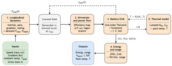
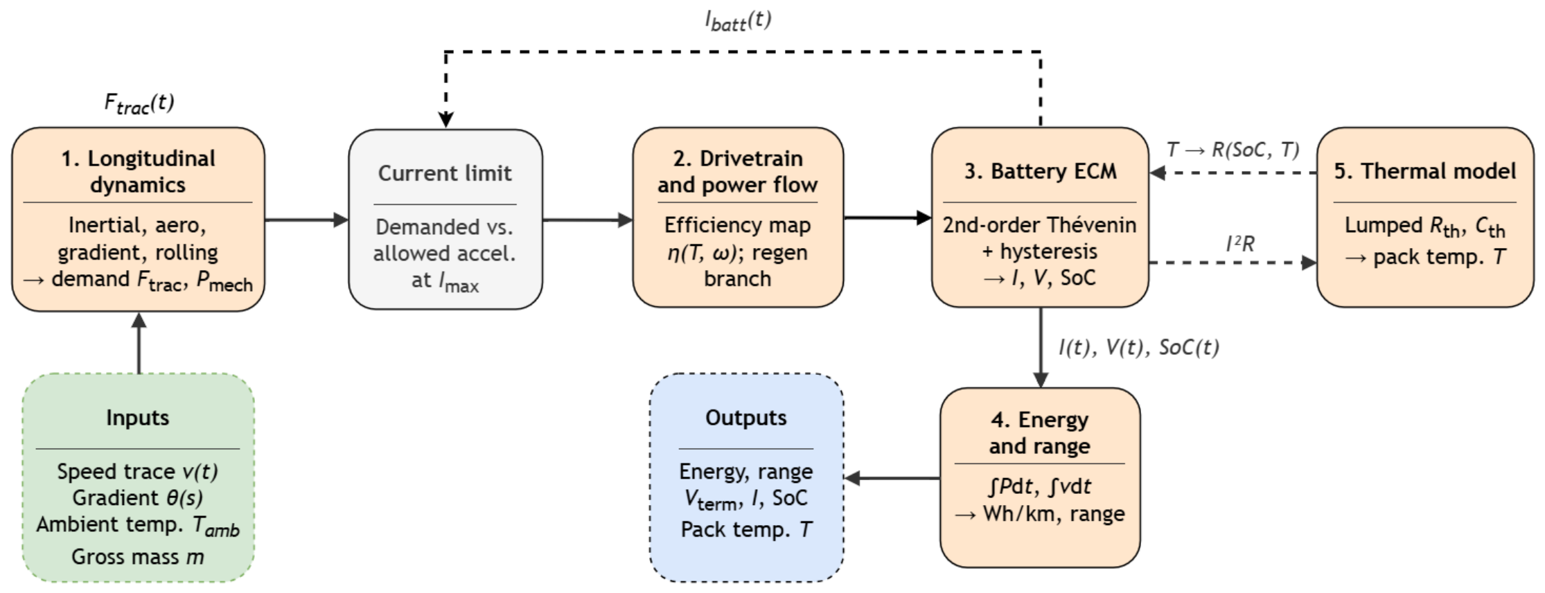
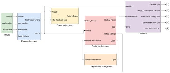
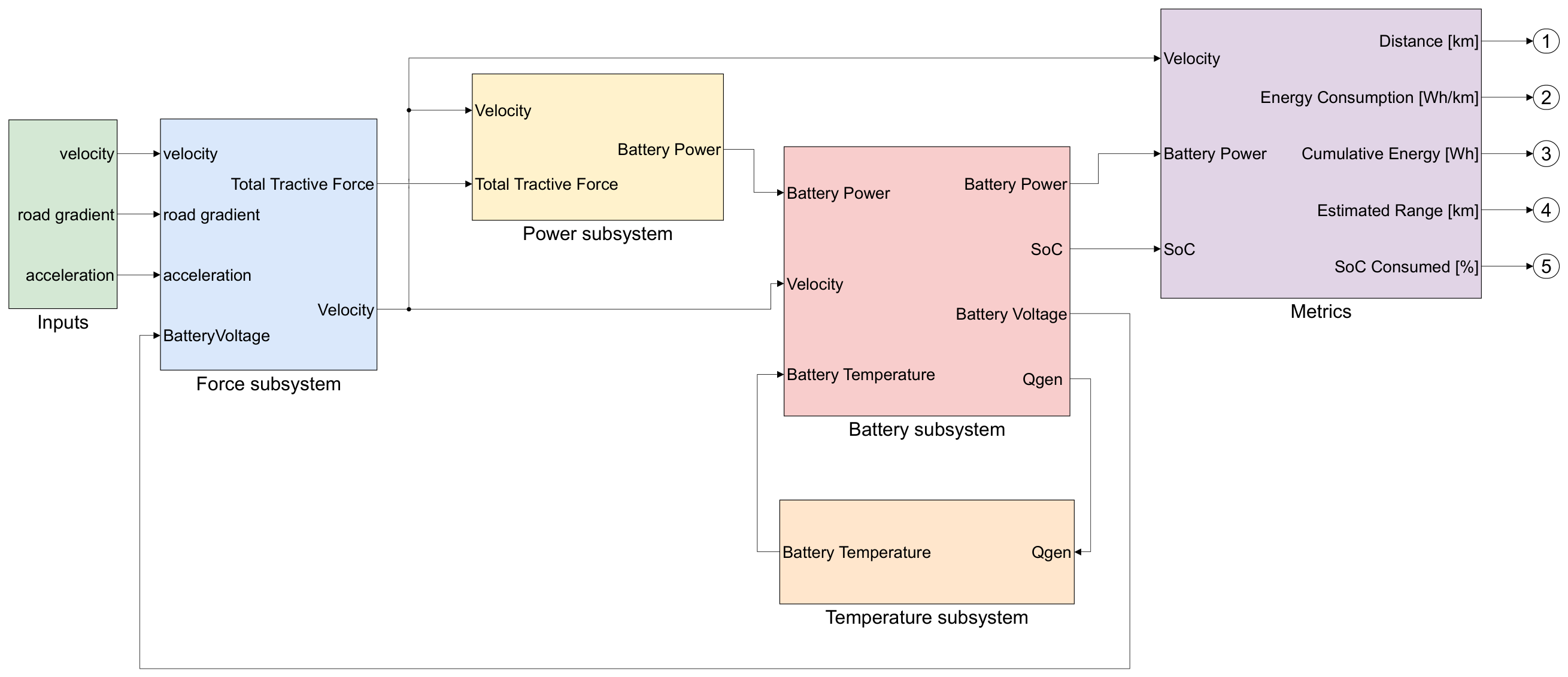
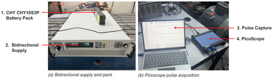
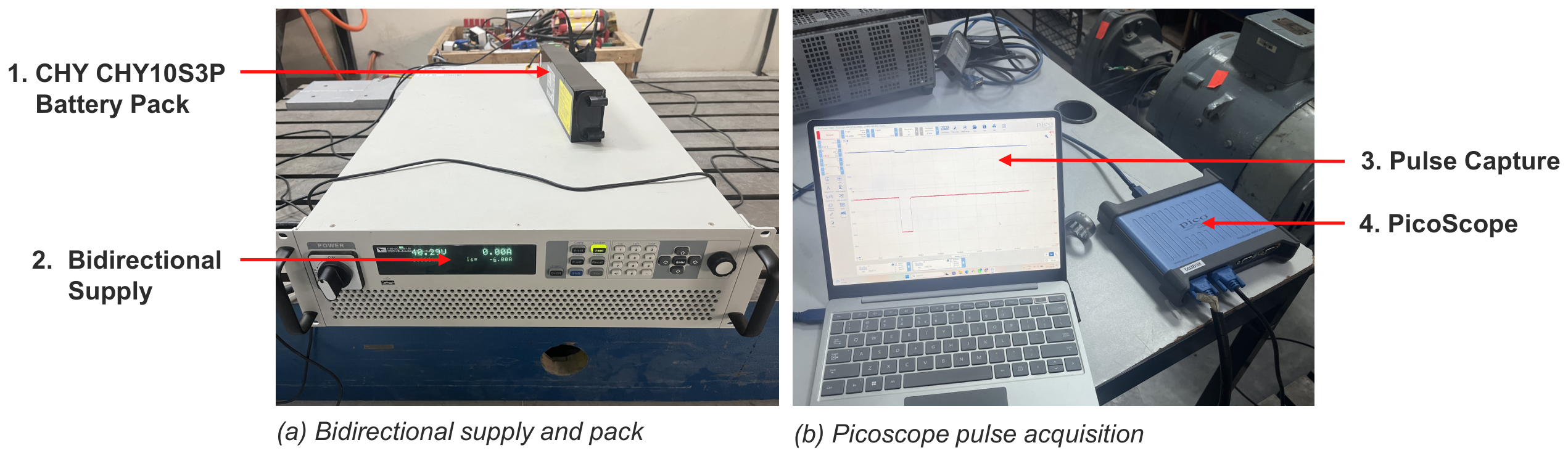
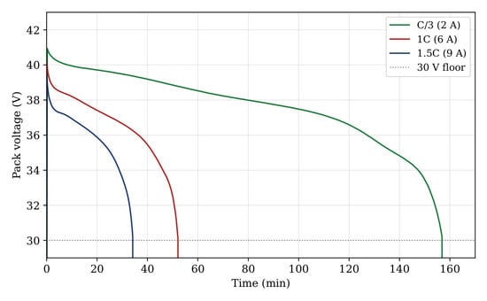
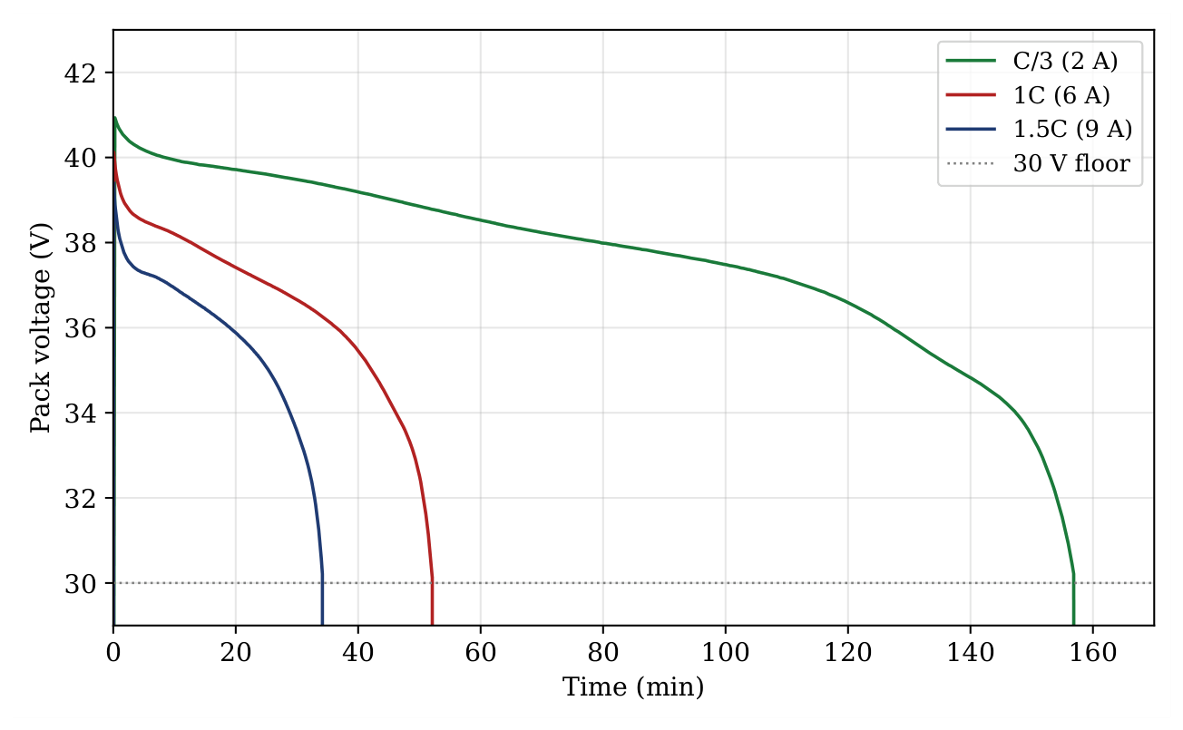
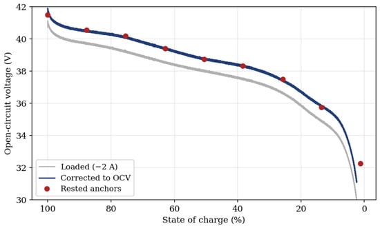
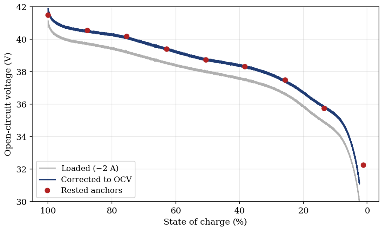
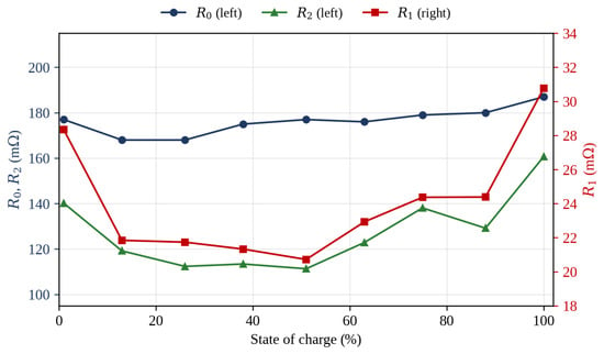
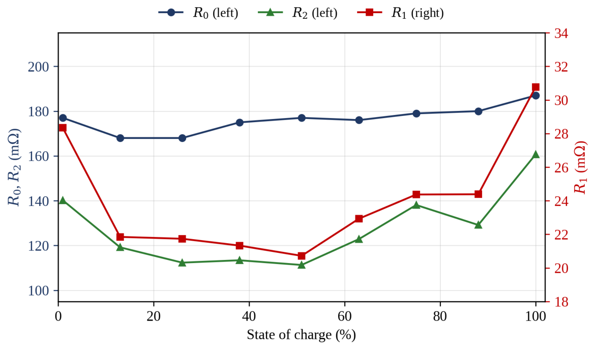
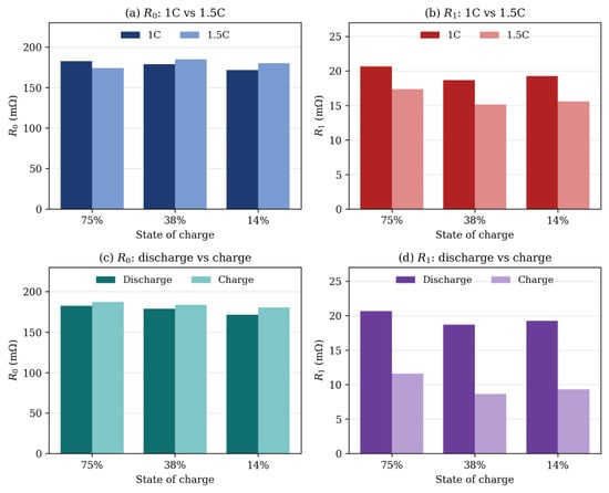
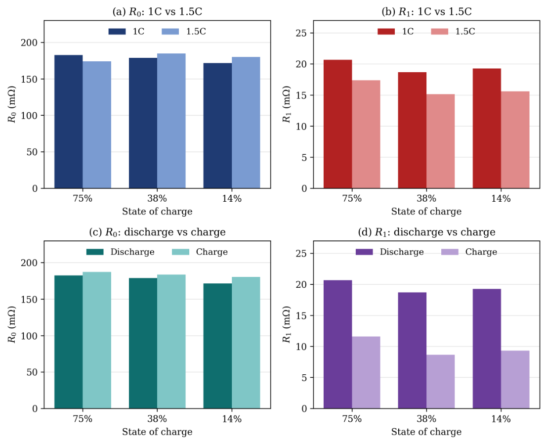
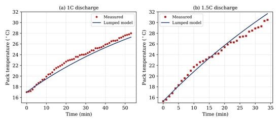
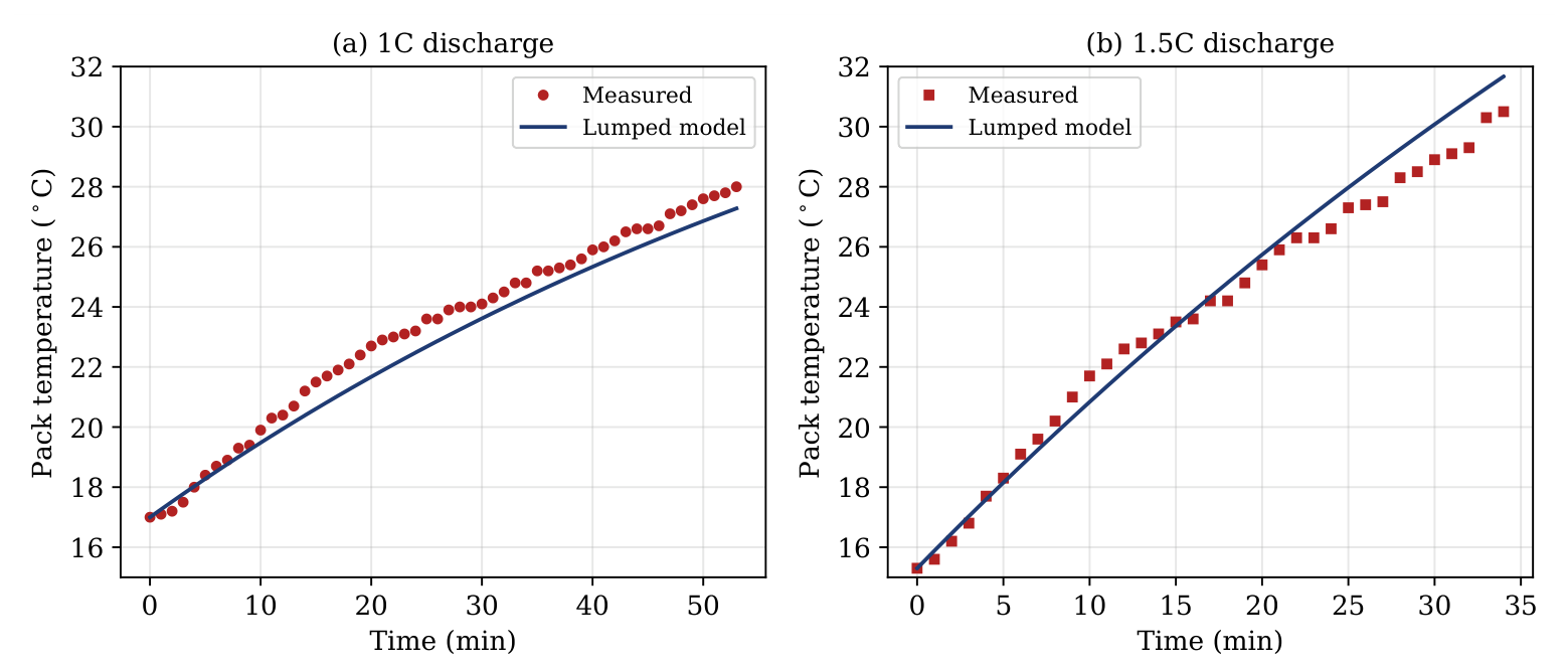
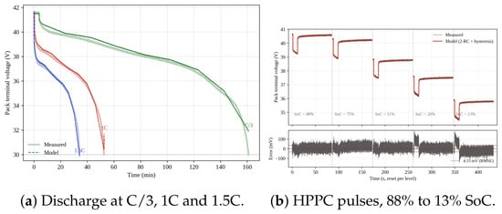
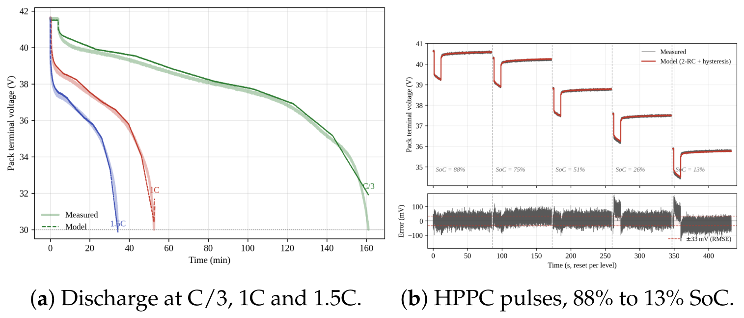
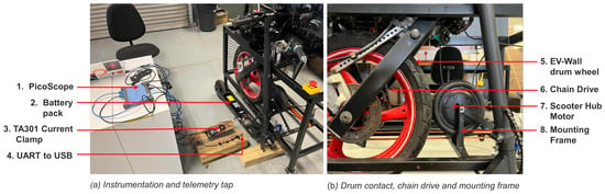
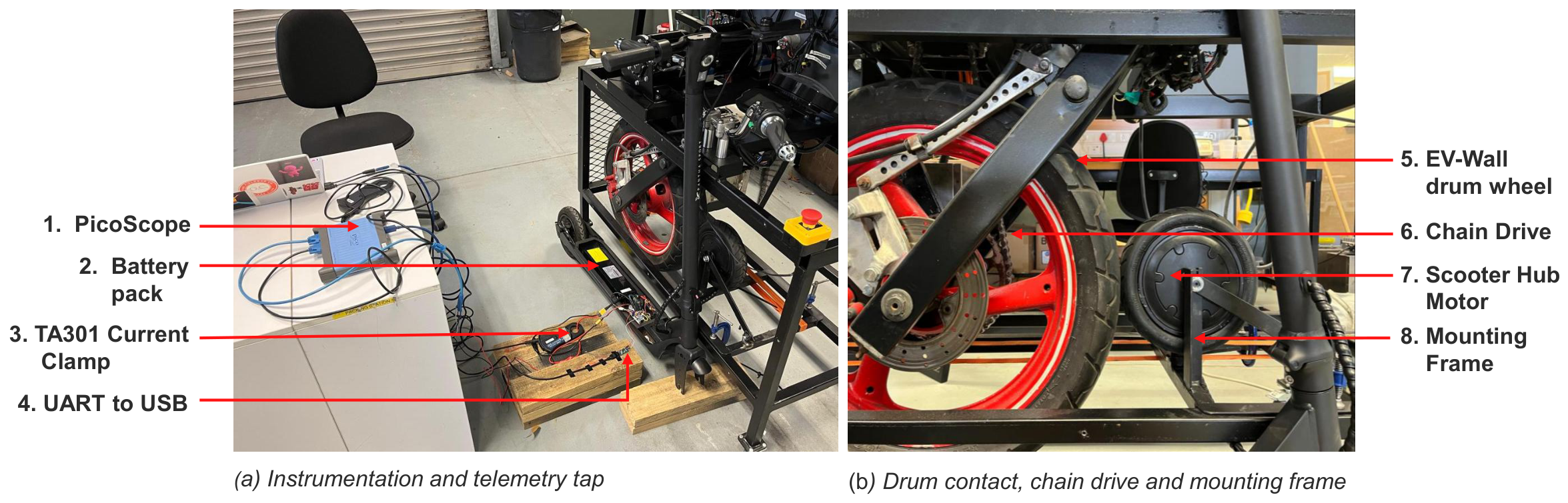
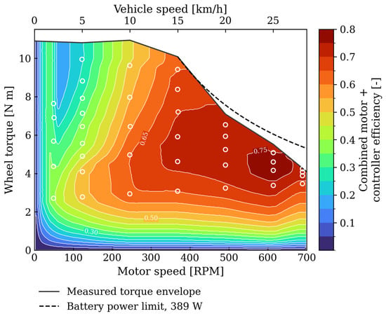
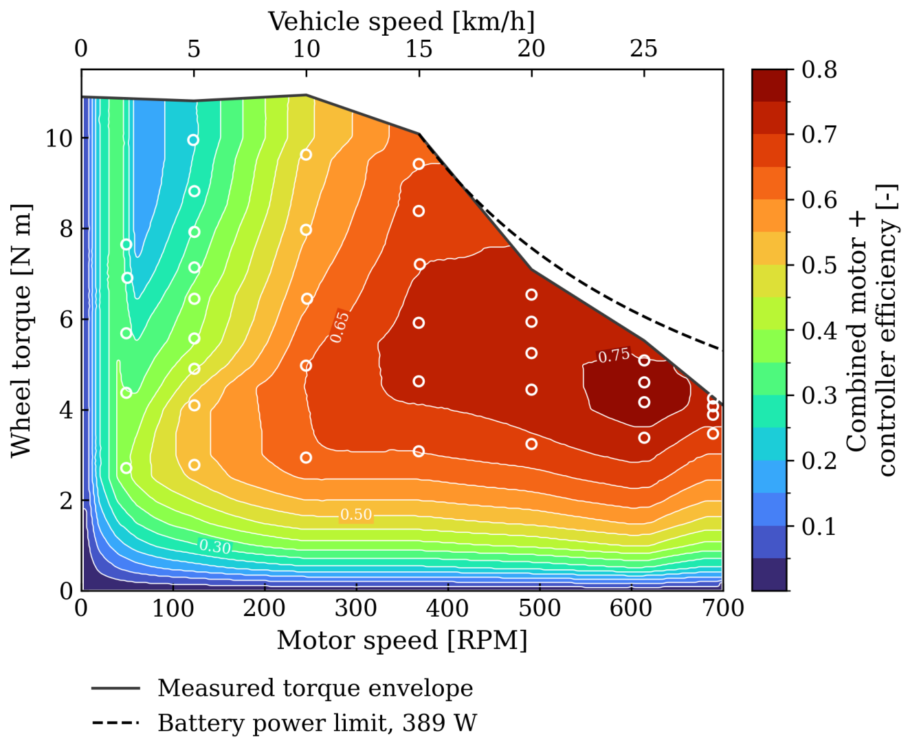
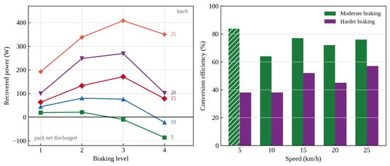
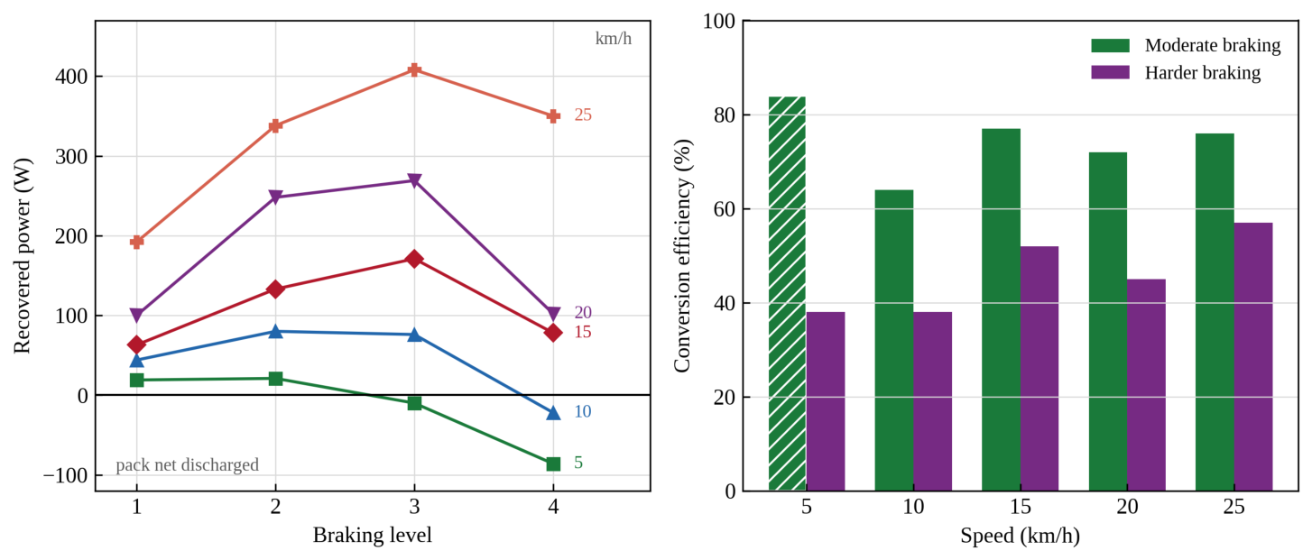
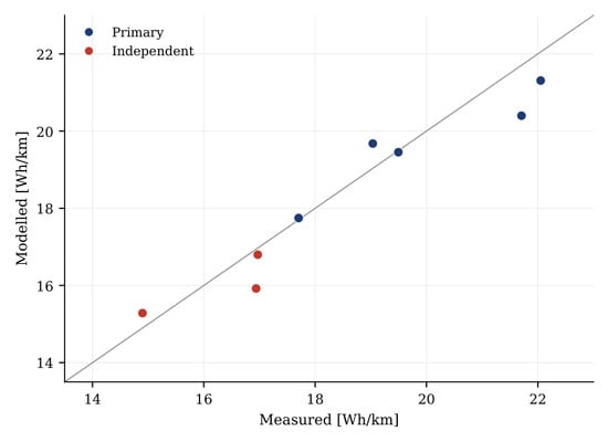
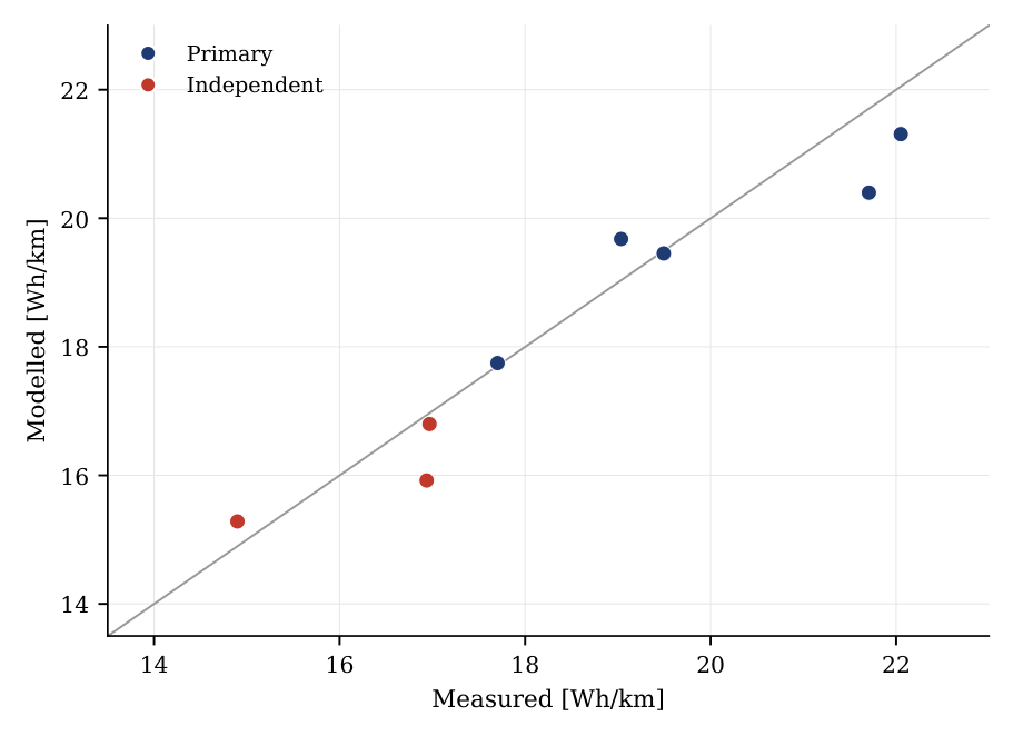
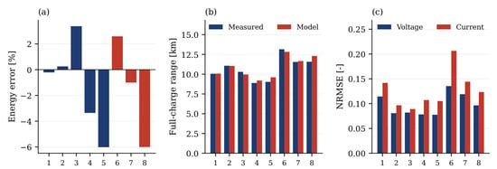
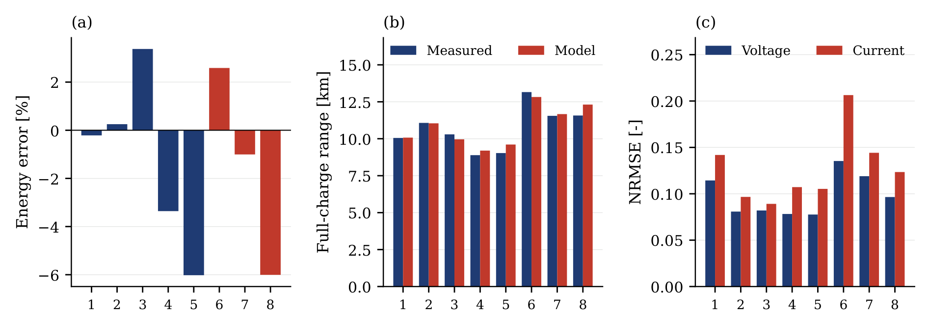
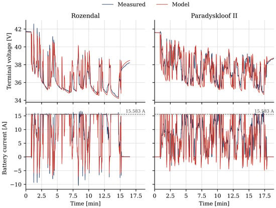
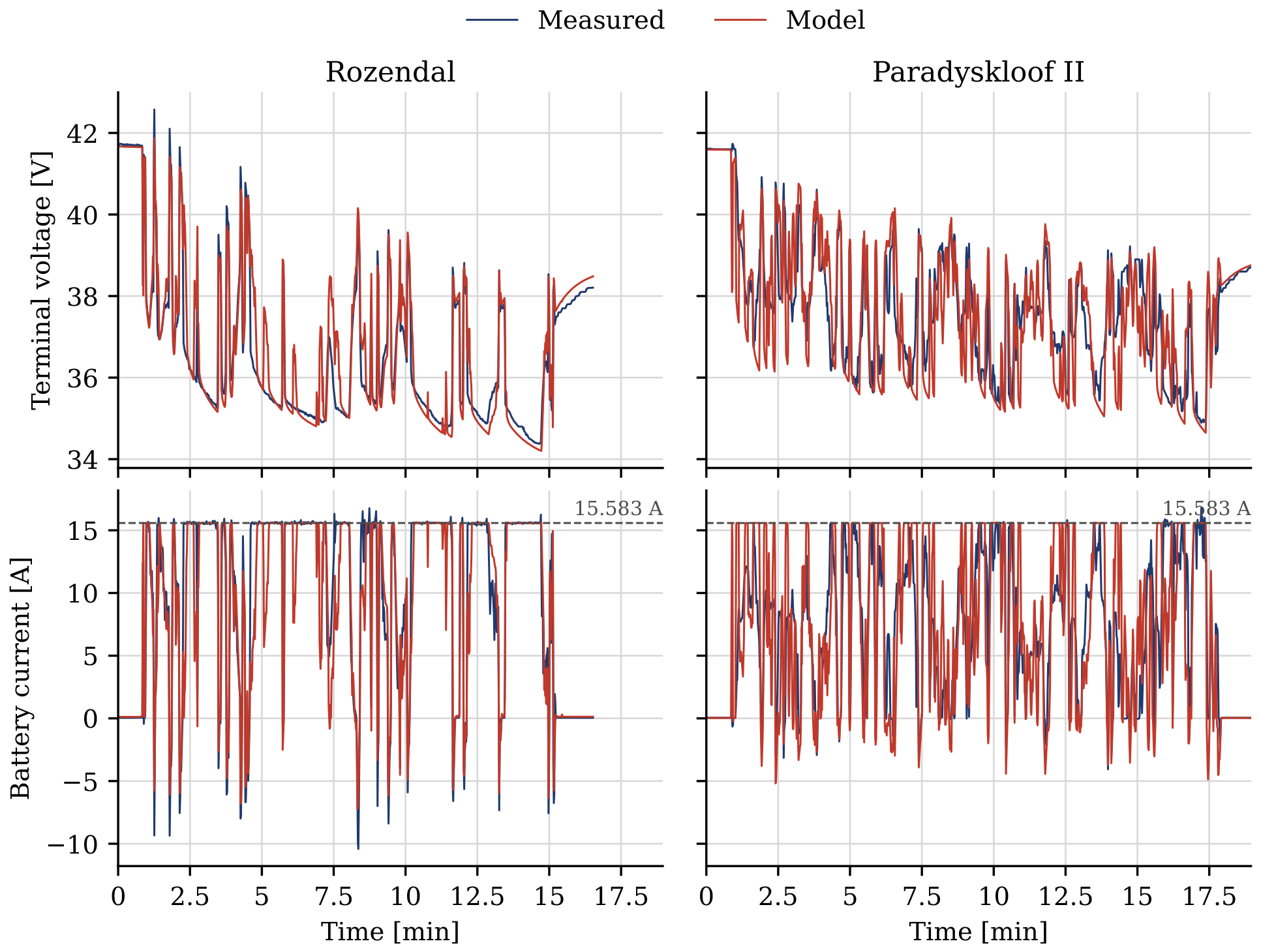
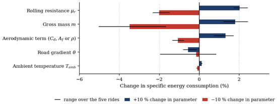
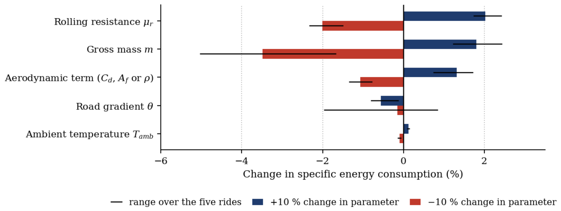

Disclaimer/Publisher’s Note: The statements, opinions and data contained in all publications are solely those of the individual author(s) and contributor(s) and not of MDPI and/or the editor(s). MDPI and/or the editor(s) disclaim responsibility for any injury to people or property resulting from any ideas, methods, instructions or products referred to in the content. |
© 2026 by the authors. Published by MDPI on behalf of the World Electric Vehicle Association. Licensee MDPI, Basel, Switzerland. This article is an open access article distributed under the terms and conditions of the Creative Commons Attribution (CC BY) license.