Binocular Stereovision-Based Dynamic 3D Ear Localization and Tracking for In-Vehicle Acoustic Applications

Highlights

What are the main findings?

• Binocular stereo vision with coarse-to-fine detection and adaptive Kalman filtering localizes and tracks passenger ears in 3D under simplified laboratory conditions.
• Progressive SIFT matching with saliency pre-screening and Kalman-constrained search reduces stereo-matching computational overhead in the tested cases.

What are the implications of the main findings?

• The deterministic, training-free pipeline offers a practical front-end candidate for future in-vehicle acoustic applications such as ANC and personal sound zones.
• Adaptive covariance and re-detection help sustain ear tracking under motion and illumination changes, supporting reliable in-vehicle acoustic control input.

Abstract

This paper presents a binocular stereovision method for reconstructing the three-dimensional spatial coordinates of the occupant’s ear, as a laboratory proof-of-concept for future in-vehicle acoustic applications. The binocular system is calibrated using a two-step radial alignment constraint. For robust detection, a coarse-to-fine cascade fuses skin-color, geometric, and contour features, where the skin-color model updates online with a forgetting factor to adapt to illumination while contour matching outputs a confidence score. Scale-invariant feature transform points are extracted and ranked by importance, and stereo-matching is guided by a Kalman-predicted dynamic search window. Match verification is achieved via nearest-neighbor ratio, epipolar geometric consistency, and disparity continuity. An adaptive Kalman filter smooths target positions on the two-dimensional image planes, after which smoothed coordinates are triangulated into three-dimensional spatial coordinates. Both process and observation noise covariances are adaptively adjusted according to estimated acceleration and detection confidence, and the Mahalanobis distance triggers a full-image re-detection upon tracking loss. Experimental results for a seated participant under simplified in-vehicle conditions show tracking accuracy within five millimeters and a progressive stereo-matching time of about forty-five milliseconds. These results support the feasibility of the proposed framework for future in-vehicle acoustic applications.

1. Introduction

The design focus of intelligent vehicle cockpits is expanding beyond the driver to encompass all occupants. Auditory perception is a key dimension of ride comfort, which positions the ear’s spatial coordinates as a fundamental input for multiple in-vehicle functional modules. For instance, active noise control (ANC) requires establishing a local quiet zone around the ear to achieve low-frequency noise reduction [1,2]. Tseng [3] showed that for a 108 Hz pure tone, an elliptical quiet zone of approximately 0.35 m × 0.35 m × 0.6 m can be obtained, yet this zone shrinks rapidly as the frequency rises. Once the occupant’s head deviates from the preset position, the noise reduction performance degrades noticeably, implying that ANC must acquire the ear coordinates in real time to reposition the quiet zone. Jiang et al. [4] investigated the accuracy requirements of ear positioning for active road noise control, showing that about 2.0 cm positioning accuracy is needed for 9 dBA original reduction and 3 dBA allowable loss. Zhang [5] proposed a monocular method for binaural 3D localization and dynamic tracking in vehicle cabins, using facial landmarks and monocular depth estimation. Personal sound field systems create independent listening zones across seats using loudspeaker arrays [6,7], and spatial audio rendering requires dynamic beam steering based on binaural positions [8]; in-vehicle voice interaction demands reliable speech capture in multi-occupant, high-noise environments [9,10], where head orientation provides valuable guidance for microphone-array beamforming. Beyond these, functions such as collision out-of-position detection [11], active headrest adjustment [12], driver fatigue monitoring [13], intelligent air supply [14], and personalized audio equalization [15] also rely on occupant head pose information. Despite their functional diversity, these applications share the same underlying requirement: real-time, accurate, markerless access to the occupant’s ear coordinates in the vehicle’s three-dimensional (3D) space.

However, existing in-vehicle perception solutions are mostly configured for individual functions, with little coordination among them. Seat position estimation usually relies on seat track travel and anthropometric models for indirect calculation. While cost-effective, it fails to capture real-time posture changes and individual variations. Depth cameras can also directly output three-dimensional data, yet their depth information is prone to failure under direct sunlight, and their field of view is limited. In contrast, the hardware setup of monocular vision is the simplest, but two-dimensional images lack depth information, causing errors to escalate sharply when occupants move fore and aft. Although marker-based motion capture systems have the highest accuracy, they require attached markers and are impractical in real-world vehicular scenarios. Within the monocular vision framework, previous studies have attempted to detect ear regions using image segmentation [16], skin-color models [17], contour features [18], and AdaBoost classifiers [19]. These methods, however, remain essentially confined to two-dimensional image processing and struggle to recover three-dimensional spatial coordinates. Therefore, a common limitation of these approaches is that each is designed for a single application, and few simultaneously satisfy the combined requirements of accuracy, real-time performance, and convenience across multiple scenarios.

Within purely vision-based approaches, the trade-off between accuracy and computational efficiency remains a central challenge. Deep learning-based detectors paired with dense stereo-matching deliver precise results, but the computational cost is considerable; for instance, state-of-the-art foundation models for stereo-matching require hundreds of milliseconds per frame, and even lightweight variants often exceed 50 ms on resource-constrained platforms [20]. Lightweight methods based on skin color or simple features run considerably faster, yet they tend to be fragile under varying illumination and cluttered backgrounds. Moreover, for in-vehicle ANC systems, low-latency processing is essential, as delays directly impair cancelation performance. Sound field rendering demands even tighter accuracy. The challenge is to reconcile these competing demands with the limited computing power available onboard [21]. To this end, binocular stereovision recovers depth from disparity. The constituent modules include camera calibration [22], feature extraction [23], and stereo-matching [24], which are by now well studied. However, most existing work is set in the context of robotic navigation or general-purpose vision [25,26,27]. Systematic studies that consider the specific characteristics of the in-vehicle environment, including lighting conditions, spatial constraints, and the target itself, are scarce. A further complication is that most stereo-matching algorithms assume a static scene [28]. Additionally, during actual driving, the occupant’s head seldom remains perfectly stationary; even small movements degrade the matching rate and cause the estimated coordinates to jitter. Kalman filtering has been used to smooth the output [29], yet this relies on noise covariance matrices, which fail to adapt to varying motion dynamics or fluctuating observation quality.

To address these limitations, this paper proposes a binocular stereovision method for dynamic tracking of the occupant’s ear in three-dimensional space, which integrates detection, matching, and tracking. It is intended as a unified perceptual input for potential future cockpit audio applications. The framework combines skin-color detection, scale-invariant feature transform (SIFT) matching, and Kalman filtering. This combination is computationally efficient, requiring no labeled data, making it potentially suitable for future onboard implementation. Three specific improvements are made. In the detection stage, a coarse-to-fine cascade is used. Skin-color prior provides an initial coarse localization that rapidly removes a large portion of the background. Geometric constraints filter the candidates. Contour matching refines the position and outputs a confidence score. The skin-color model is not static; a forgetting factor is introduced to adapt gradually to changes in illumination. In the matching stage, feature points are first ranked by importance. Only the top-ranked ones are retained for matching, reducing the computational load. The search window is constrained by the Kalman-predicted position, and its size is adjusted dynamically according to prediction uncertainty. A triple-check mechanism, including nearest-neighbor distance ratio, epipolar geometric consistency enforced by the pre-calibrated fundamental matrix, and disparity continuity, is applied to ensure matching quality. In the tracking stage, an adaptive Kalman filter is used. The process noise covariance is adjusted in real time based on acceleration estimates to reflect changes in the occupant’s motion. The observation noise covariance adapts to detection confidence. If the Mahalanobis distance exceeds a threshold, tracking is considered lost and a full-image re-detection is triggered.

The present study develops a laboratory proof-of-concept framework for future in-vehicle acoustic applications. It uses a deterministic, training-free binocular stereovision method for dynamic 3D ear localization and tracking, integrating adaptive skin-color detection, progressive SIFT matching, and adaptive Kalman filtering, and is evaluated under simplified in-vehicle conditions with a seated participant performing typical head-turning motions. The main contributions are threefold:

(1)

A coarse-to-fine cascade detection strategy is developed, integrating adaptive skin-color prior, geometric constraints, and contour matching to improve ROI extraction under the tested illumination variations.

(2)

A multi-strategy progressive stereo-matching method is proposed, incorporating importance-based feature pre-screening and a Kalman-predicted dynamic search window to reduce computational overhead.

(3)

An adaptive Kalman filter is designed with covariance adaptation driven by both motion acceleration and detection confidence, complemented by a loss-of-track re-detection mechanism.

2. System Configuration and Calibration

2.1. Establishment of Binocular Stereovision System

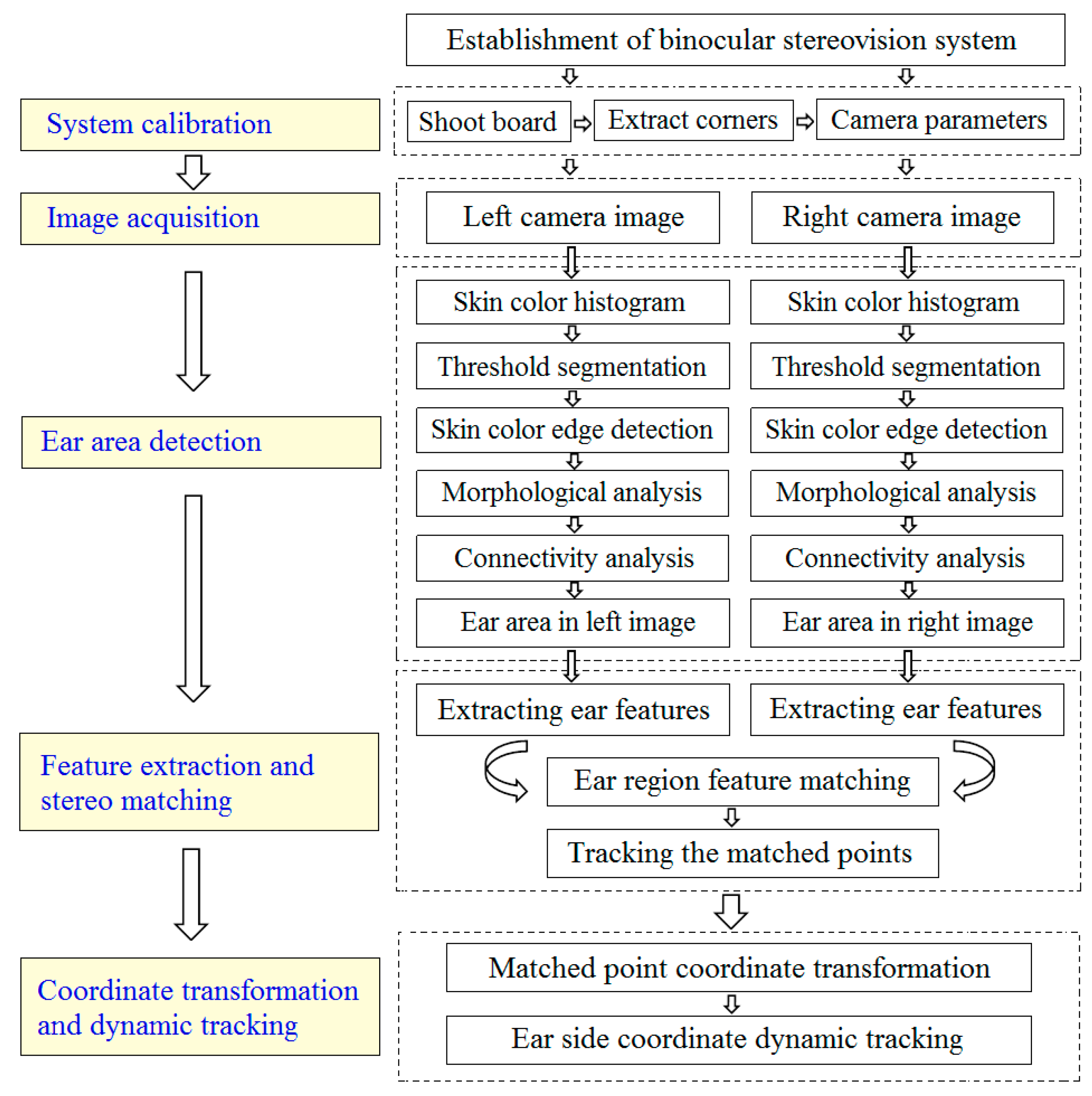
To obtain the 3D spatial coordinates of the occupant’s ear, a binocular stereovision system is established. The overall workflow is organized into four stages, as shown in Figure 1. The first stage is system calibration using the two-step radial alignment constraint (RAC) method [30]. The second stage is ear area detection, where skin-color histogram, adaptive threshold segmentation, edge detection, morphological operations, and connectivity analysis are sequentially applied to identify the ear region in both left and right images. The third stage is feature extraction and stereo-matching using SIFT features, KD-tree search, and RANSAC-based outlier rejection. The final stage is coordinate transformation and dynamic tracking, where matched points are projected to 3D world coordinates and tracked by a Kalman filter over consecutive frames.

Figure 1. Schematic diagram of dynamic recognition for spatial coordinates of occupant’s ears.

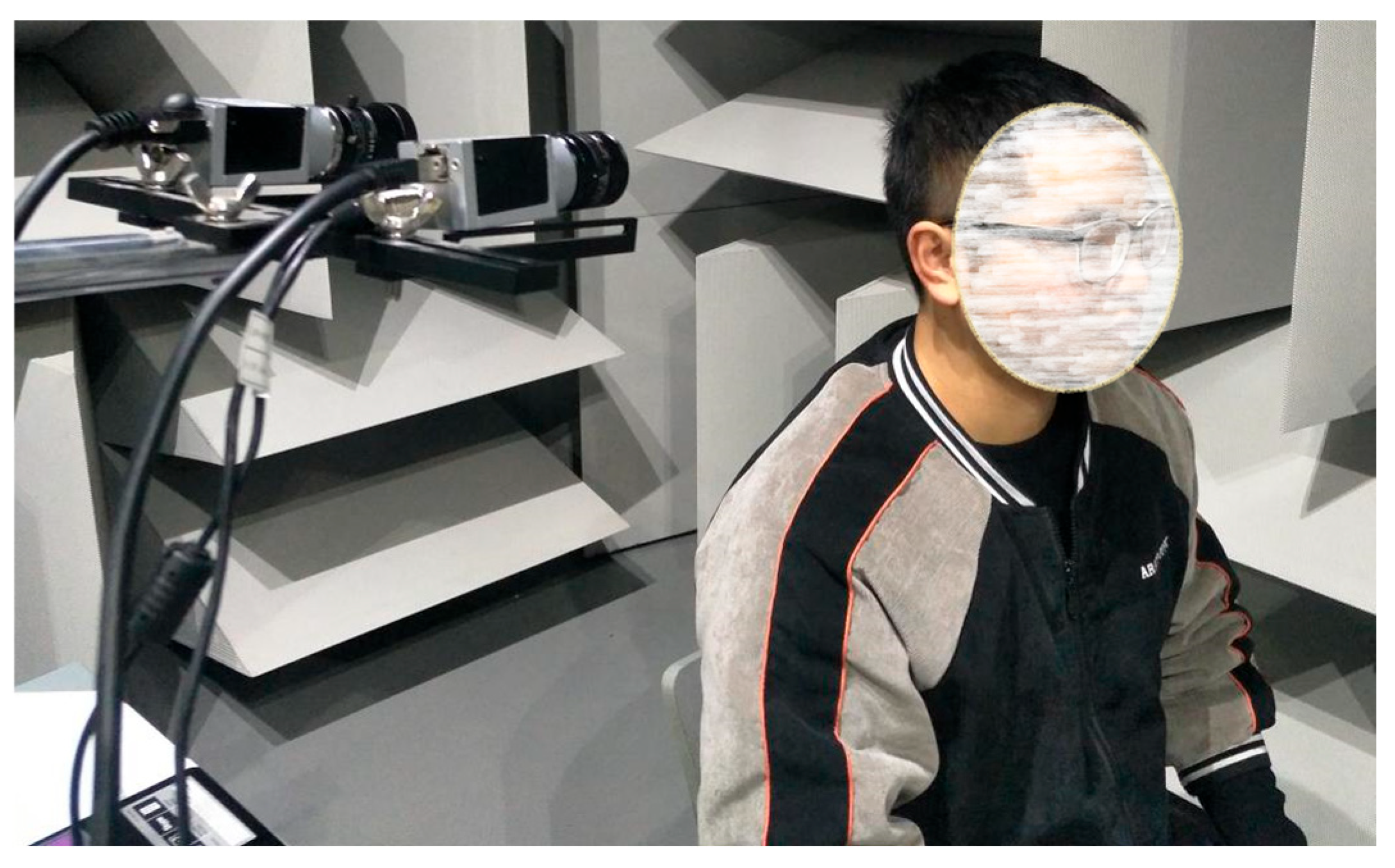
The hardware system is built around two charge-coupled device (CCD) cameras, supported by a calibration board, a computer, and an image acquisition card. The cameras capture synchronized images of the occupant’s head from two viewpoints, and the images are transferred to the computer via the acquisition card for subsequent processing. Figure 2 shows the hardware configuration, and Table 1 summarizes the camera specifications. Key installation parameters include the focal length, baseline length, and pitch angle. Based on the distance from the cameras to the occupant’s ear area and the required field of view, the focal length is set to 12 mm. The cameras are mounted as high as possible within the cabin to increase the field of view, and their optical axes are kept parallel to minimize distortion. Considering the trade-off between parallax accuracy and matching difficulty, a baseline length of 150 mm is adopted. The pitch angle is determined by the expected head motion range. A standard checkerboard pattern is used as the calibration board, and the calibration images are processed on the same computer to obtain the camera parameters.

Figure 2. Setting of the binocular vision system.

Table 1. Camera parameters.

Parameter	Resolution	Pixel Size	Frame Rate	Gain Range	Exposure Time Range
Value	2594 × 2048	4.8 µm × 4.8 µm	22 fps	0–10 dB	10 µs–10 s

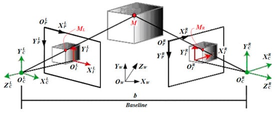
To transform 2D image coordinates to 3D spatial coordinates, four reference frames are defined: the world coordinate system (W), camera coordinate system (C), image coordinate system (I) and pixel coordinate system (P). Their relationships are illustrated in Figure 3. The origin O_W of the world coordinate system W is set at the geometric center of the left camera, the Z_W axis points to the travel direction of a vehicle, and the Y_W axis is perpendicular to the horizontal plane. The camera coordinate system C has its origin O_C at the optical center, with Z_C as the optical axis. The image coordinate system I has its origin O_I at the principal point, with X_I and Y_I parallel to X_C and Y_C, respectively; the distance from O_I to O_C is the focal length f. The pixel coordinate system P has its origin at the top-left corner of the image, with the U-axis pointing right and the V-axis pointing down. For a target point M with coordinates (x_C, y_C, z_C), its projections on the left and right image planes are M_L and M_R, with image coordinates (x_IL, y_IL) and (x_IR, y_IR), respectively. Under parallel optical axes, y_IL = y_IR. The disparity is defined as d = x_IL − x_IR. By similar triangles, the 3D coordinates of point M are obtained as

x_C = b ⋅ x_IL/d,y_C = b ⋅ y_IL/d,z_C = b ⋅ f/d

(1)

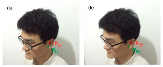
where b is the baseline length between the two cameras. Figure 4 shows typical stereo images of the occupant’s head captured by the left and right cameras, where the points P_L1 and P_L2 in the left image correspond to P_R1 and P_R2 in the right image, respectively. All human faces in the article are from one of the authors. By constructing the corresponding relationship between the left and right images, one may calculate the disparity d, and thereby obtain 3D coordinates of the ear area.

Figure 3. Relationships among the defined four coordinate systems of W, C, I and P.

Figure 4. The binocular images obtained by the (a) left and (b) right cameras.

2.2. Calibration for Binocular Stereovision System

To accurately obtain three-dimensional information about the passenger’s ear, the binocular stereovision system must be calibrated. The two-step method based on the RAC algorithm is adopted due to its computational efficiency and robustness. The parameters of calibration are summarized in Table 2, where α_x and α_y are scale factors, γ is the non-vertical factor, u₀ and v₀ are the optical centers, k is the radial distortion coefficient, and R and T are the external rotation matrix and translation vector, respectively.

Table 2. The internal and external camera parameters of the binocular stereovision system.

Internal Parameter	Expressions	External Parameter	Expressions
Perspective transformation	$A=\left[\begin{array}{ccc}{\alpha }_x& \gamma & u_0\\ 0& {\alpha }_y& {\nu }_0\\ 0& 0& 1\end{array}\right]$	Translational matrix	$R=\left[\begin{array}{ccc}{r}_1& r_2& r_3\\ r_4& r_5& r_6\\ r_7& r_8& r_9\end{array}\right]$
Radial distortion	k	Rotational matrix	$T={\left[\begin{array}{ccc}{t}_x& t_y& t_z\end{array}\right]}^T$

Assuming that the spatial coordinates of a projection point P are (x_W, y_W, z_W), its corresponding coordinates in the camera coordinate system are (x_C, y_C, z_C), and can be calculated as

$$\left[\begin{array}{c}{x}_C\\ y_C\\ z_C\end{array}\right]=R\left[\begin{array}{c}{x}_W\\ y_W\\ z_W\end{array}\right]+T$$

(2)

where T is a translational vector matrix with a dimension of 3 × 1, R is an orthogonal transformation matrix with a dimension of 3 × 3. The rotation matrix is parameterized by the roll angle ψ, the yaw angle Φ, and the pitch angle θ as

$$R=\left[\begin{array}{ccc}\cos \phi \cos \theta & \cos \phi \sin \theta \sin \psi -\sin \phi \cos \psi & \cos \phi \sin \theta \cos \psi +\sin \phi \sin \psi \\ \sin \phi \cos \theta & \sin \phi \sin \theta \sin \psi +\cos \phi \cos \psi & \sin \phi \sin \theta \cos \psi -\cos \phi \sin \psi \\ -\sin \theta & \cos \theta \sin \psi & \cos \theta \cos \psi \end{array}\right]$$

(3)

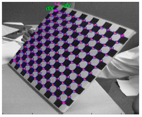
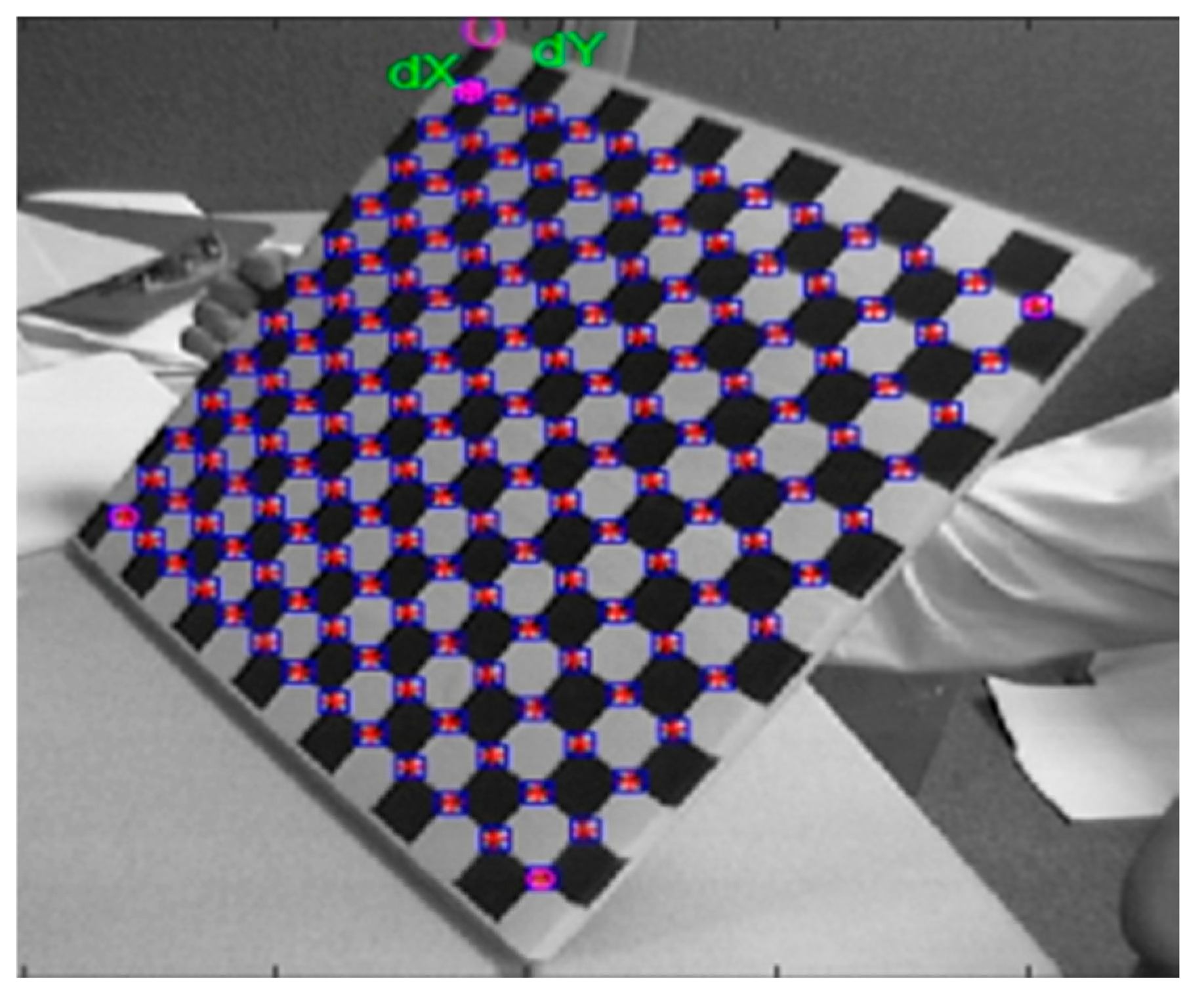
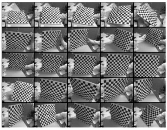
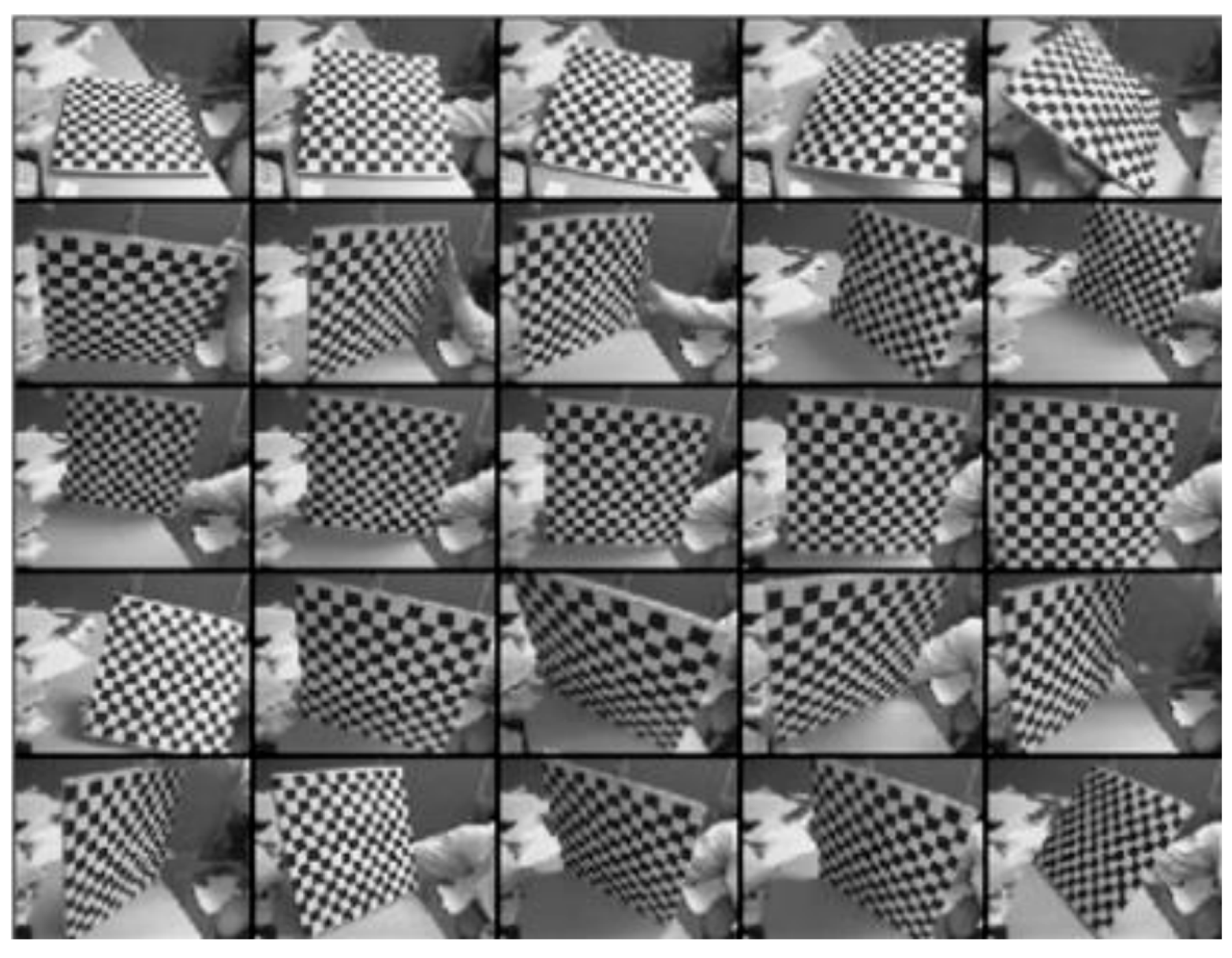
Multi-position calibration experiments are conducted based on the RAC algorithm. A checkerboard calibration target with 12 × 13 grids, each 30 mm × 30 mm in size, is designed as shown in Figure 5. A corner window size of 5 mm × 5 mm is used for corner detection. For each camera, 25 images are captured from different orientations, as shown in Figure 6, and 156 corner points are extracted as reference data. The two-step RAC calibration procedure is as follows.

Figure 5. A board designed for multi-position calibration.

Figure 6. Image acquisitions for camera calibration.

From the extracted board corner points, N feature points with pixel coordinates (X_fi, Y_fi), i = 1, 2, …, N, are obtained. Assuming a feature point p_i corresponds to the world coordinate (x_Wi, y_Wi), the actual image coordinates (X_di, Y_di) after lens distortion can be calculated as

X_di = (X_fi − X_c)/N_x,Y_di = (Y_fi − Y_c)/N_y

(4)

where (X_c, Y_c) is the image center coordinate and (N_x, N_y) are the pixel counts per unit length on the image plane.

From the RAC conditions and the relationship between the rotational matrix R and the coordinates (x, y, z), the following linear equation is derived

$$\left[\begin{array}{cccc}\begin{array}{cc}{x}_{\mathit{Wi}}{Y}_{\mathit{di}}& y_{\mathit{Wi}}{Y}_{\mathit{di}}\end{array}& Y_{\mathit{di}}& -x_{\mathit{Wi}}{X}_{\mathit{di}}& -y_{\mathit{Wi}}{X}_{\mathit{di}}\end{array}\right]\left[\begin{array}{c}\begin{array}{c}{r}_1/t_y\\ r_2/t_y\end{array}\\ t_x/t_y\\ r_4/t_y\\ r_5/t_y\end{array}\right]=X_{\mathit{di}}$$

(5)

Using the least square method to solve the overdetermined system, the variables $r_1^{\prime }=r_1/t_y$, $r_2^{\prime }=r_2/t_y$, $t_x^{\prime }=t_x/t_y$, $r_4^{\prime }=r_4/t_y$ and $r_5^{\prime }=r_5/t_y$ are obtained. Based on the orthogonality of the rotation matrix and the right-handed coordinate convention, the full rotation matrix R is recovered. Let $s_r^{\prime }=s_1^{\prime 2}+s_2^{\prime 2}+s_4^{\prime 2}+s_5^{\prime 2}$ and S = −sgn(r₁r₄ + r₂r₅), then,

$$t_y^2={\displaystyle \frac{s_r^{\prime }-\sqrt{s_r^{\prime 2}-4{(r_1^{\prime }{r}_5^{\prime }-r_2^{\prime }{r}_4^{\prime })}^2}}{2{(r_1^{\prime }{r}_5^{\prime }-r_2^{\prime }{r}_4^{\prime })}^2}}$$

(6)

Taking a positive value of t_y, the following are obtained: $r_1=r_1^{\prime }{t}_y$, $r_2=r_2^{\prime }{t}_y$, $r_3=\sqrt{1-r_1^2-r_2^2}$, $r_4=r_4^{\prime }{t}_y$, $r_5=r_5^{\prime }{t}_y$, $r_6=\sqrt{1-r_4^2-r_5^2}$, and $t_x=t_x^{\prime }{t}_y$. The remaining elements r₇, r₈ and r₉ are then computed from the orthogonality constraints.

For the extrinsic parameter calibration, the intrinsic parameters are fixed. According to Equation (2), the coordinates (x_i, y_i, z_i) of each feature point p_i are

$$\left\{\begin{array}{c}{x}_i=r_1{x}_{\mathit{Wi}}+r_2{y}_{\mathit{Wi}}+t_x\\ y_i=r_4{x}_{\mathit{Wi}}+r_5{y}_{\mathit{Wi}}+t_y\\ z_i=r_7{x}_{\mathit{Wi}}+r_8{y}_{\mathit{Wi}}+t_z\end{array}\right.$$

(7)

Let Q_i = r₇x_wi + r₈y_wi. If y_i = r₄x_wi + r₅y_wi + t_y, then

$$\left[y_i-(Y_{\mathit{fi}}-Y_c)/N_y\right]\left[\begin{array}{c}f\\ t_z\end{array}\right]=(Y_{\mathit{fi}}-Y_c)Q_i/N_y$$

(8)

Substituting the calculated effective focal length f and translational component t_z into the following equations,

$$\left\{\begin{array}{c}{X}_{\mathit{ui}}(1+k{\gamma }^2)=f{x}_i/z_i\\ Y_{\mathit{ui}}(1+k{\gamma }^2)=f{y}_i/z_i\end{array}\right.$$

(9)

where (X_ui, Y_ui) are the undistorted image coordinates in the ideal linear camera model, and the radial distortion coefficient k is determined. Thus, the internal and external parameters of the binocular cameras are fully determined. The obtained parameters and re-projection errors for the left and right cameras are summarized in Table 3 and Table 4. The opposite sign in Table 3 arises from the image rectification pipeline. During preprocessing, the right camera image is horizontally flipped to align the epipolar geometry with the left camera. Under the adopted RAC convention, the radial distortion model is applied after this flip, which reverses the sign of the radial coordinate relative to the image center, yielding k_L ≈ −0.0956 and k_R ≈ +0.0955. After applying the corresponding sign compensation in the rectification step, the epipolar alignment residual remains below 0.3 pixels, which is sufficient for the subsequent matching stages.

Table 3. The determined internal parameters of binocular cameras.

Internal Parameters	Left Camera	Right Camera
Effective focal length	[972.45, 972.41]	[975.51, 975.22]
Optical centers [u0, v0]	[613.82, 490.93]	[621.67, 487.29]
Radial distortion k	−0.09563	0.09547
Non-vertical factor γ	0	0
Re-projection error	[0.2542, 0.2658]	[0.2814, 0.2849]

Table 4. The determined external parameters of binocular cameras.

External Parameters	Left Camera	Right Camera
Rotational matrix R	$\left[\begin{array}{ccc}-0.936& -0.0173& 0.332\\ 0.0071& -0.986& 0.0019\\ 0.3213& 0.0013& 0.9438\end{array}\right]$	$\left[\begin{array}{ccc}-0.864& -0.0152& 0.318\\ 0.0067& -0.9436& 0.0024\\ 0.3146& 0.0016& 0.8962\end{array}\right]$
Translational matrix T	${\left[\begin{array}{ccc}-52.136& 5.280& 99.460\end{array}\right]}^T$	${\left[\begin{array}{ccc}-50.200& 5.160& 95.200\end{array}\right]}^T$

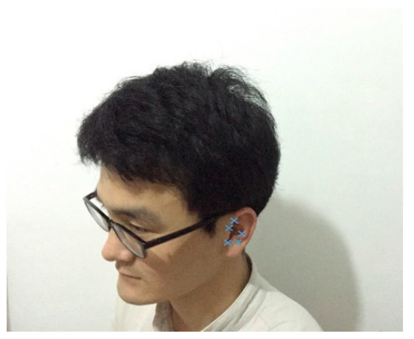
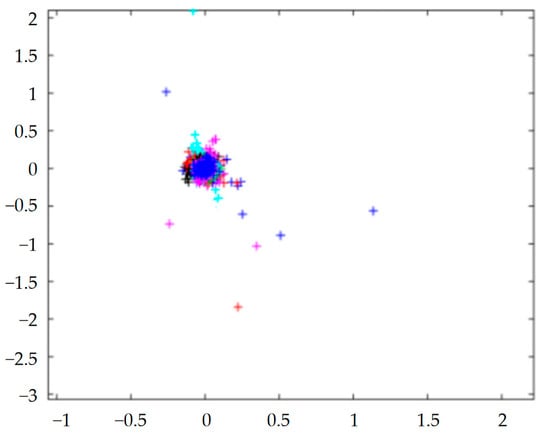
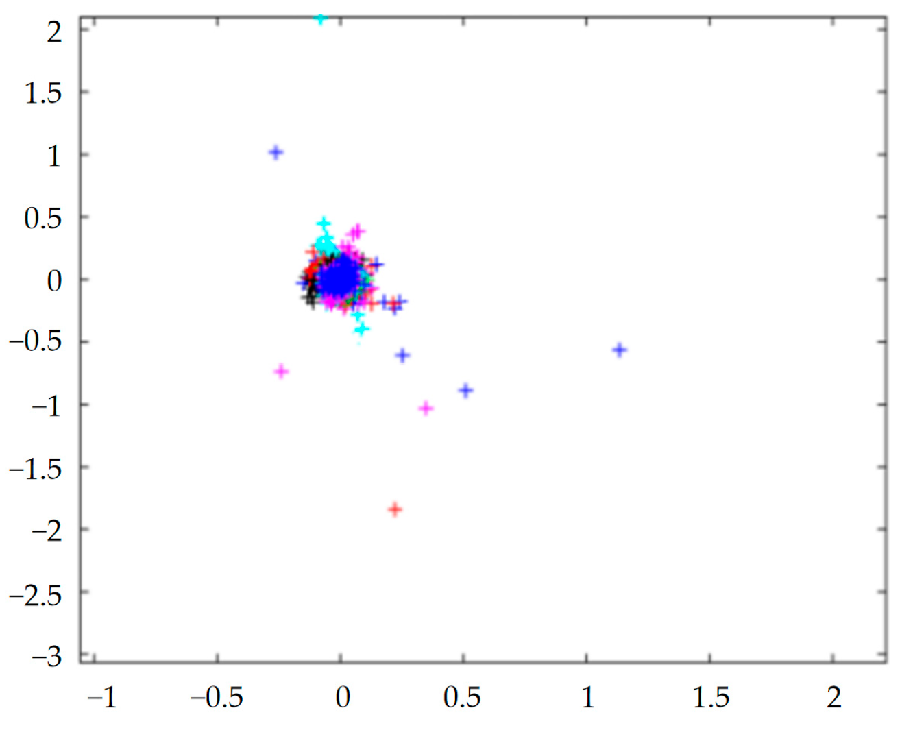
Using the calibrated parameters, feature points of the occupant’s ear in Figure 4 are extracted and shown in Figure 7. The resulting 3D spatial coordinates are compared with ground-truth measurements. The re-projection errors are analyzed following [31], and the results are presented in Figure 8. The error distribution is relatively concentrated, indicating that the RAC-based calibration yields reasonable and consistent results. The calibrated binocular stereovision system is therefore suitable for subsequent ear detection, recognition, and tracking.

Figure 7. The extracted feature points at the occupant’s ear side.

Figure 8. A plot of re-projection errors.

3. Multi-Feature Fusion for Ear Detection

To reduce the computational complexity of subsequent stereo-matching and coordinate extraction, a multi-feature fusion detection method is developed to identify the ear region in the left and right images. The method integrates skin-color, geometric, and contour features within a unified probabilistic framework that outputs a confidence score for each detection.

3.1. Online Skin-Color Modeling with Forgetting Factor

The skin-color prior is established using a histogram model in a suitable color space. To accommodate gradual illumination changes in the vehicle cabin, the skin-color model is updated online rather than fixed after initialization. Skin-color distribution is relatively stable under moderate head movement and facial expression for the tested participant, making it a useful basis for coarse ear localization.

Let H_t (k) denote the normalized skin-color histogram at frame t for the k-th color bin. The histogram is updated via exponential weighted moving average

$$H_t(k)=\lambda \cdot H_{t-1}(k)+(1-\lambda )\cdot {\widehat{H}}_t(k)$$

(10)

where ${\hat{H}}_t(k)$ is the observed histogram from the current frame, and λ ∈ (0, 1) is the forgetting factor that controls the adaptation rate. A larger λ emphasizes historical information for stability under steady illumination, while a smaller λ accelerates adaptation to sudden lighting changes. In this study, λ = 0.9 was selected over the range [0.8–0.95]. This value provides a balance between detection stability under steady illumination and adaptability to gradual lighting changes.

Based on the updated histogram, the likelihood of a pixel belonging to the skin region is computed via back-projection, and adaptive threshold segmentation extracts the candidate skin areas. The adaptive threshold segmentation is formulated as follows. Assuming an image of size M × N with the grayscale value f(i, j) at pixel (i, j), the original image histogram h(k) after normalizing is H(k). After valley width darkening and peak generation, it becomes h_b1(k) and h_b2(k); thus,

$$h(k)={\displaystyle \sum _{i=0}^{M-1}{\displaystyle \sum _{j=0}^{N-1}\delta \left\{f(i,j)-k\right\}}}$$

(11)

$$h_{b1}(k)={\displaystyle \sum _{i=0}^{M-1}{\displaystyle \sum _{j=0}^{N-1}g\left\{e(i,j)\right\}·\delta \left\{f(i,j)-k\right\}}}$$

(12)

$$h_{b2}(k)={\displaystyle \sum _{i=0}^{M-1}g{\displaystyle \sum _{j=0}^{N-1}\left\{e(i,j)\right\}·\delta \left\{f(i,j)-k\right\}}}/H(k)$$

(13)

where δ(·) is the unit pulse function, e(i, j) is the gradient edge operator, and g{e(i, j)} is a monotonic descent function,

$$e(i,j)={\displaystyle \underset{x,y=-1}{\overset{1}{\max }}}\left\{f(i-x,j-y)\right\}-{\displaystyle \underset{x,y=-1}{\overset{1}{\min }}}\left\{f(i-x,j-y)\right\}$$

(14)

g{e(i,j)} = [1 + e(i,j)]⁻²

(15)

After normalizing, the h_b1(k) and h_b2(k) are denoted as H_b1(k) and H_b2(k). A new histogram h_b0(k) is obtained:

h_b0(k) = H_b1(k) + H_b2(k)

(16)

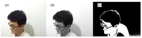
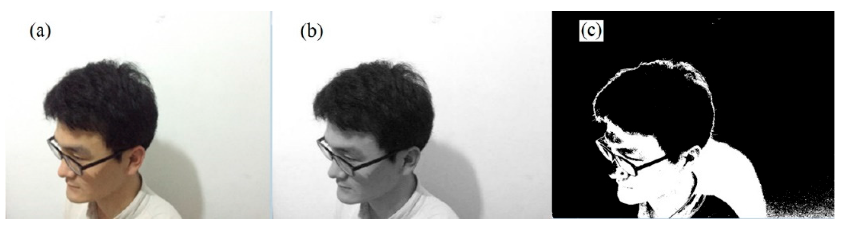
The histogram H_b0(k) after adaptive threshold segmentation can be obtained by normalizing the h_b0(k). Figure 9 shows the segmentation results of skin-color areas from the adaptive threshold segmentation method. The image areas of the ear and other parts with similar skin color (face, hairline, shadow) are separated from the backgrounds, but an effective separation of the ear has not yet been achieved. Therefore, further edge detection, morphological processing, and connectivity analysis are necessary to achieve accurate ear detection.

Figure 9. The results of threshold segmentation: (a) original image, (b) skin-color conversion, (c) threshold segmentation.

3.2. Coarse-to-Fine Cascade Detection with Bayesian Verification

The detection strategy is formulated as a hierarchical Bayesian decision process organized in a coarse-to-fine cascade.

Stage 1—Coarse localization: The online skin-color model generates candidate regions R₀ with an initial prior probability P(R₀). Regions with skin-color likelihood below a preset threshold are discarded, rapidly removing a large portion of the background.

Stage 2—Geometric constraint filtering: Geometric priors of the human ear are applied as a likelihood function P(G|R), where G denotes geometric attributes including aspect ratio, area, and solidity. Instead of using fixed numerical intervals, a frame-wise relative ranking is adopted. For each frame, all candidate regions are sorted in descending order of their aspect ratio (height/width of the minimum enclosing rectangle). The top N = 3 candidates are retained as ear candidates, while the rest are discarded. This relative-order criterion adapts to frame-wise variations in head pose and distance without requiring predefined aspect-ratio bounds.

Stage 3—Contour matching for refinement: For the remaining candidates, edge contours are extracted using the wavelet modulus maximum algorithm. For a smoothing function θ(x,y) satisfying ∫∫_Rθ(x,y)dxdy = 1, its partial derivatives in x and y directions can be regarded as two-dimensional wavelet functions.

$${\psi }^x(x,y)={\displaystyle \raisebox{1ex}{$\partial \theta (x,y)$}\!\left/ \!\raisebox{-1ex}{$\partial x$}\right.}, {\psi }^y(x,y)={\displaystyle \raisebox{1ex}{$\partial \theta (x,y)$}\!\left/ \!\raisebox{-1ex}{$\partial y$}\right.}$$

(17)

For any function f(x, y) ∈ L²(R), the wavelet transform components at scale s are

$$W_s^{x}f(x,y)=f·{\Psi }_s^x(x,y),W_s^{y}f(x,y)=f·{\Psi }_s^y(x,y)$$

(18)

The gradient vector is defined as

$$\left[\begin{array}{c}{W}_s^{x}f(x,y)\\ W_s^{y}f(x,y)\end{array}\right]=s\overrightarrow{\nabla }(f*{\theta }_s)(x,y)$$

(19)

The modulus and argument of wavelet transform can be calculated by

$$M_{s}f(x,y)=\sqrt{\left|W_s^{x}f{(x,y)}^2+W_s^{y}f{(x,y)}^2\right|}$$

(20)

$$A_{s}f(x,y)=\mathit{arctg}\left[{\displaystyle \frac{W_s^{x}f(x,y)}{W_s^{y}f(x,y)}}\right]$$

(21)

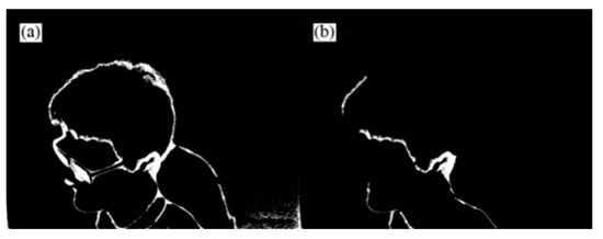
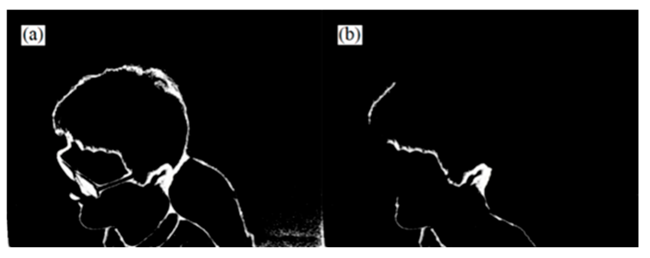
where the modulus M_sf(x,y) is proportional to the gradient value, and the argument A_sf(x,y) is the angle between the gradient vector and the horizontal direction, pointing to the image edge. The edge detections are performed on the image after adaptive threshold segmentations, and the obtained edge images at different scales are overlaid. Figure 10a shows the overlaid edge image. For removing interferences, a further edge area search is performed, and the results are shown in Figure 10b, where the obtained edge image has partly removed facial and background edges but still contains some interference areas.

Figure 10. The results of edge detection: (a) edge image, (b) edge image after removing interferences.

The detected contours are then compared with an ear shape template through chamfer matching. The ear shape template was constructed from a representative side-view image of the primary participant. The contour was manually verified and stored as a binary shape template. The matching residual e_contour, which is the root mean square error of aligned contour points, is mapped to a detection confidence score c ∈ [0, 1]

$$c={\displaystyle \frac{1}{1+\exp (\alpha \cdot e_{\mathit{contour}}+\beta )}}$$

(22)

where the mapping function is calibrated to produce a higher score for closer contour alignment. This confidence score is normalized to the [0, 1] interval; higher values indicate stronger agreement with the ear template and are used to reduce the observation noise covariance in the subsequent Kalman filter (Section 5.3), while lower values trigger a more conservative filtering update. The operating threshold is fixed for all experiments.

To eliminate edge interferences, the edge image is further processed by morphological operations. Mathematically, erosion and dilation are defined as

AΘB = {(x|B_x ∩ A^c}

(23)

$$A\oplus B=\left\{\left.z\right|{\overline{B}}_z\cap A\right\}$$

(24)

The opening and closing operations are defined as A∘B = (AΘB)⊕B and A·B = (A⊕B)ΘB, respectively. Figure 11 shows the results of image morphological processing and refinements. From the open operation and the first refinement results in Figure 11a,b, the open operation separates the ear from the surrounding areas, and the first refinement eliminates the smaller areas in the image. From the close operation and the second refinement results in Figure 11c,d, the internal area of the ear is filled and enclosed, and secondary refinement transforms the edge line of the ear into a single-pixel curve.

Figure 11. The results of image morphological processing and refinements: (a) open operation, (b) first refinement, (c) close operation, and (d) second refinement.

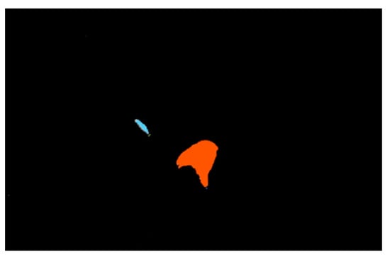
Connectivity analysis using the region-growing method separates individual skin-color blobs. Figure 12 shows the connectivity analysis results of skin-color regions, where each generated block is marked by a color. After connectivity analysis, the regions are independent and have different shapes, which can be further screened through the minimum enclosing rectangles with different aspect ratios.

Figure 12. The result of connectivity analysis.

After connectivity analysis, each independent skin-color connected component is obtained. To distinguish the ear region from other skin-colored parts (e.g., neck, cheek, or forearm), a topological shape prior is adopted instead of fixed numerical interval rules. For each connected component, the aspect ratio of its minimum enclosing rectangle is computed. Rather than applying a predefined constant threshold, all components are sorted in descending order of this ratio within the current frame. This ranking-based criterion is based on the observation that, in lateral or near-lateral views of a seated occupant, the ear region tends to exhibit greater vertical elongation than other visible skin-colored areas under typical head pose ranges. Components with higher ranks in this sorted list are retained as ear candidates, whereas those with lower ranks are discarded. This relative-order criterion adapts to frame-wise variations in head pose and illumination without requiring fixed aspect-ratio bounds. The retained top-ranked candidates are then passed to the subsequent contour matching stage. At this initial screening stage, the primary objective is to maintain high recall (i.e., to avoid irreversible misses), while the rejection of false positives is progressively accomplished in the subsequent stages. The resulting ear areas obtained via this ranking procedure are shown in Figure 13.

Figure 13. The obtained area of the occupant’s ear.

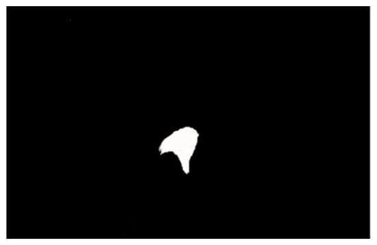
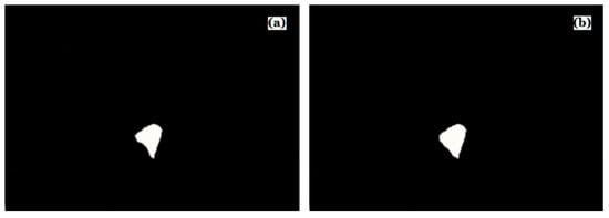
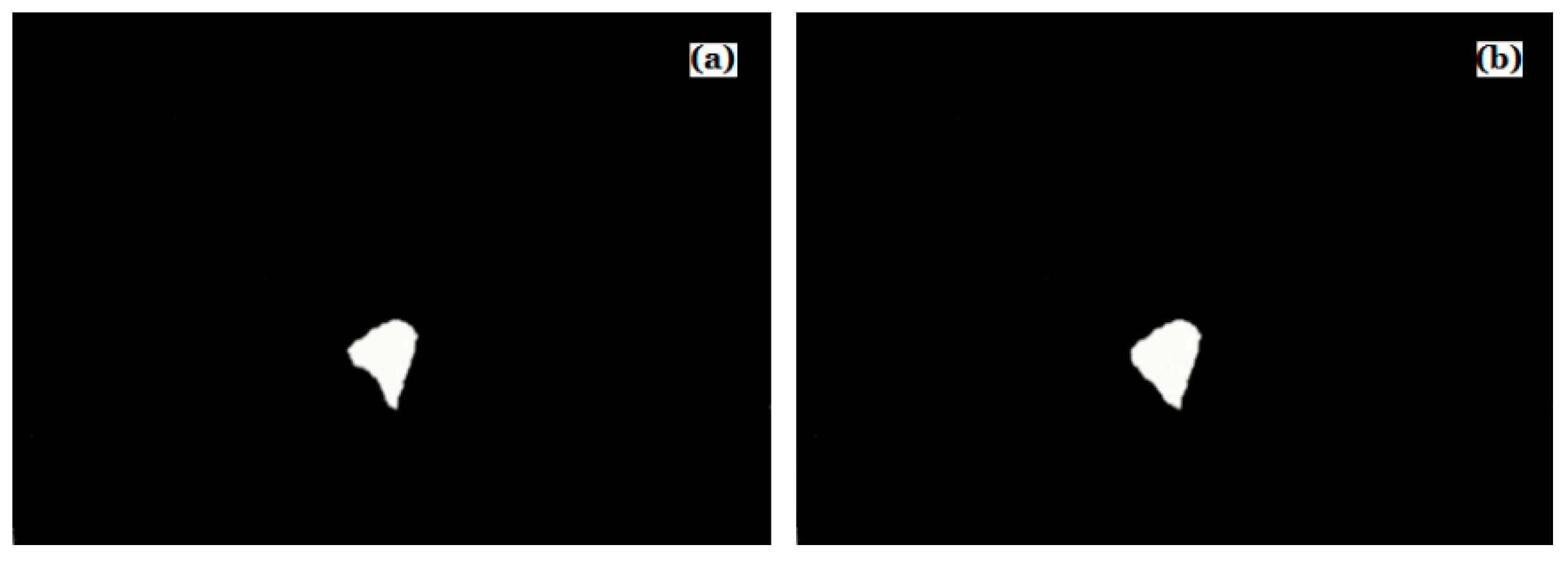
To eliminate the fine edge lines in the detected ear area, the ear area is further eroded and reconstructed, and the results are shown in Figure 14. The reconstructed white area is the finally detected ear area.

Figure 14. Results of image erosion and reconstruction: (a) eroded image, (b) reconstructed image.

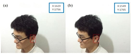
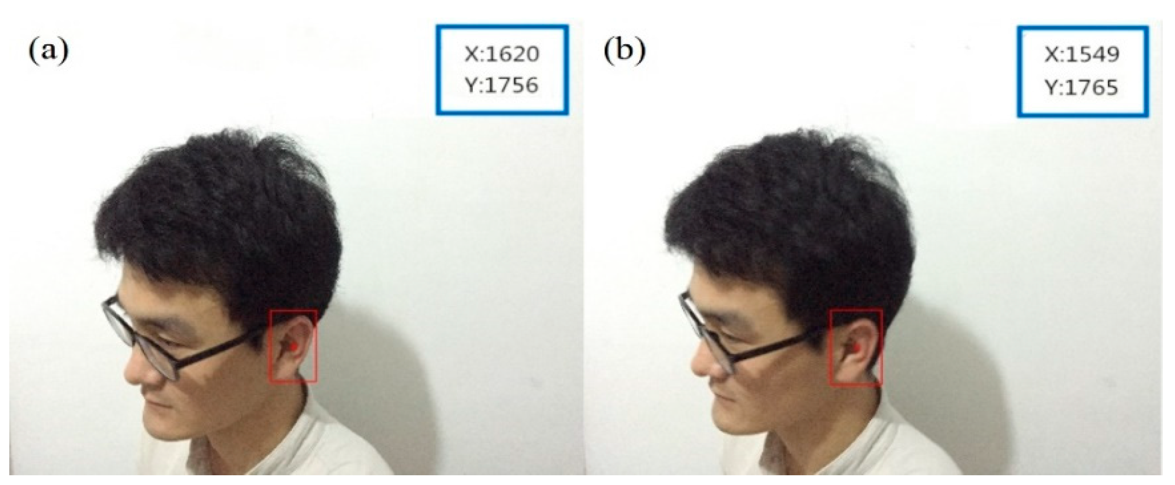
Figure 15 shows the extracted ear area results from the left and right cameras, where the red bounding box indicates the detected ear region marked with a width of five pixels, and the red dot marks the region center. This center point serves as the measurement input for the subsequent tracking stage. The confidence score c computed from contour matching is passed to the Kalman filter for adaptive observation noise adjustment.

Figure 15. The extracted results of ear area from (a) the left camera and (b) the right camera.

4. Progressive Stereo-Matching with Saliency-Guided Feature Pre-Screening

To obtain reliable correspondences between the left and right ear regions, a progressive stereo-matching method is developed. The method introduces importance-based pre-screening, Kalman-predicted search window constraint, and a triple-check verification mechanism.

4.1. Saliency-Guided Feature Pre-Screening

The SIFT algorithm is employed to extract local features from the detected ear regions. The algorithm consists of four steps: scale-space extreme point detection, keypoint localization, orientation assignment, and feature vector generation. Each extracted feature point has scale, direction, and location information, making SIFT robust to image rotation, scaling, and affine transformation.

The scale space L(u,v,σ) is constructed by convolving the input image I(u,v), with a Gaussian kernel,

L(u,v,σ) = G(u,v,σ) * I(u,v)

(25)

where ∗ is the convolution operator. The difference of Gaussian (DOG) function is used for scale-invariant keypoint detection:

D(u,v,σ) = L(u,v,kσ) − L(u,v,σ)

(26)

To reduce the amount of calculation, the DoG pyramid is used for image smoothing and alternate sampling in different scale spaces, and multi-resolution Gaussian images are generated. Comparing adjacent sampling points in the image space, the extreme points of D(u,v,σ) are determined, and their corresponding scale, direction, and location are saved. Keypoints are localized by Taylor expansion of D(u,v,σ) in scale space. For a local extreme point (u₀,v₀,σ₀), the Taylor expansion of the DOG function is

$$D(u,v,\sigma )=D(u_0,v_0,{\sigma }_0)+{\displaystyle \frac{\partial D^T}{\partial U}}U+{\displaystyle \frac{1}{2}}{U}^T{\displaystyle \frac{{\partial }^{2}D}{{\partial }^2{U}^2}}U$$

(27)

where U=(u,v,σ)^T, ${\displaystyle \frac{\partial D}{\partial U}}=\left[\begin{array}{ccc}{\displaystyle \frac{\partial D}{\partial u}}& {\displaystyle \frac{\partial D}{\partial v}}& {\displaystyle \frac{\partial D}{\partial \sigma }}\end{array}\right]$. If the derivative of D is zero, the local extreme point $\widehat{U}$ can be determined by

$$\widehat{U}=-{\displaystyle \frac{{\partial }^2{D}^{-1}}{\partial U^2}}{\displaystyle \frac{\partial D}{\partial U}}$$

(28)

Substituting Equation (28) into Equation (27) yields

$$D(\widehat{U})=D+{\displaystyle \frac{1}{2}}{\displaystyle \frac{\partial D^T}{\partial U}}$$

(29)

If $\left|D(\widehat{U})\right|<0.03$, the extreme point is discarded due to low contrast [32]. To ensure rotation invariance, the pixel gradients and directions within a 3σ neighborhood of the DoG pyramid image are used to describe the image features. The gradient magnitude and orientation are

$$m(u,v)=\sqrt{{(L(u+1,v)-L(u-1,v))}^2+{(L(u,v+1)-L(u,v-1))}^2}$$

(30)

θ(u,v) = tan⁻¹((L(u,v + 1) − L(u,v − 1))/(L(u + 1,v) − L(u − 1,v))

(31)

where m(u,v) and θ(u,v) are the modulus and direction of the gradient at keypoint (u,v); L(u,v + 1), L(u + 1,v), L(u,v − 1) and L(u − 1,v) are the grayscale values of four pixels around the keypoint (u,v), respectively.

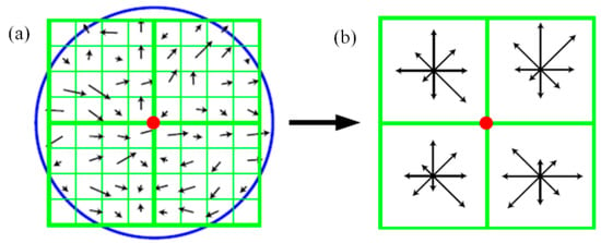
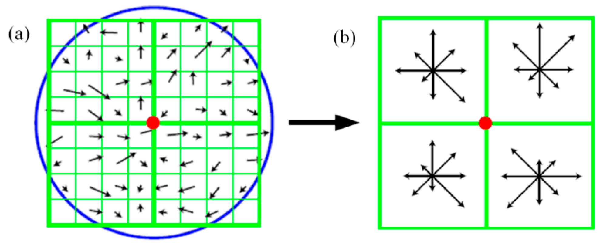
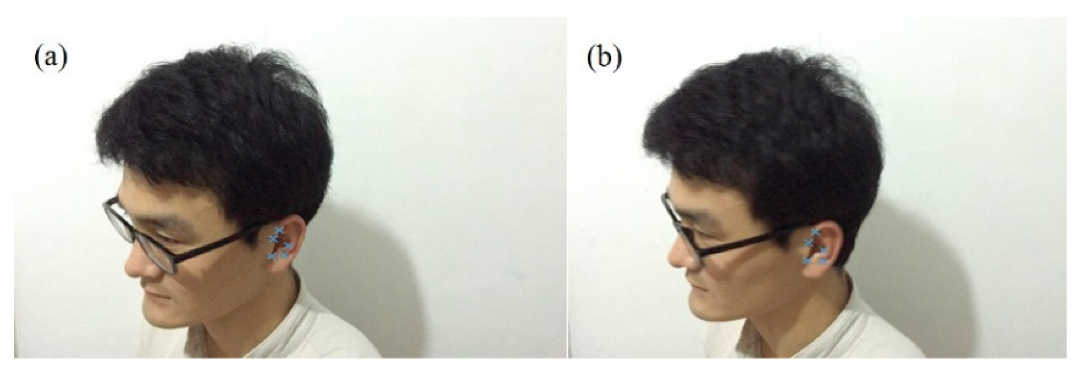
A 128-dimensional feature vector is generated for each keypoint. Taking a feature point as the center of a circle, a Gaussian window with a dimension of 8 × 8 is defined, and a seed is defined by a 4 × 4 region. Each feature point is described by 16 seeds, and each seed has 8 directional vectors, as shown in Figure 16. The feature points of the ear extracted by using the SIFT algorithm are shown in Figure 17. It can be seen that the extracted feature points are located in areas within the external contour of the ear canal, providing a foundation for subsequent stereo-matching.

Figure 16. Direction vector description of feature points: (a) image gradients around keypoint, (b) seed points.

Figure 17. The extracted feature points in the area of the occupant’s ear: (a) posture I and (b) posture II.

To reduce computational load, feature points are ranked by an importance score ω_i defined as the weighted sum of three complementary metrics

$${\omega }_i={\alpha }_{\omega }\cdot {\omega }_{\mathit{scale}}^{(i)}+{\beta }_{\omega }\cdot {\omega }_{\mathit{contrast}}^{(i)}+{\gamma }_{\omega }\cdot {\omega }_{\mathit{edge}}^{(i)}$$

(32)

where ${\omega }_{\mathit{scale}}^{(i)}=1/{\sigma }_i$ represents scale stability (smaller scales indicate finer localization); ${\omega }_{\mathit{contrast}}^{(i)}=\left|D(\widehat{U})\right|$ is the DoG response magnitude reflecting feature strength; and ${\omega }_{\mathit{edge}}^{(i)}=1/\mathit{Tr}(H)$ is the inverse of the Hessian trace used to suppress edge-like responses. The weighting coefficients α_ω, β_ω, and γ_ω satisfy α_ω + β_ω + γ_ω = 1 and are empirically balanced to favor strong corner-like structures without invoking additional entropy-based computations, thereby preserving the low-overhead nature of the pipeline.

4.2. Progressive Matching with Kalman-Predicted Search Window

After feature extraction, stereo-matching is performed to establish correspondences between feature point pairs. The KD-tree search algorithm is employed for matching point pair search. Each SIFT keypoint is represented by a 128-dimensional feature vector, and the tree structure enables efficient nearest-neighbor querying. The matching process proceeds progressively: feature points are matched starting from the highest importance scores. If the number of successful matches falls below a threshold, additional lower-ranked feature points are incrementally included until sufficient matches are obtained.

The search window for stereo-matching is dynamically constrained by the Kalman-predicted ear position rather than being fixed. Given the predicted state covariance matrix Σ_t|t−1 from the tracking stage, the search radius r_t is computed as

$$r_t=\eta \cdot \sqrt{\mathit{tr}({\Sigma }_{t|t-1})}+r_{\min }$$

(33)

where η is a scaling factor and r_min is the minimum search radius. When prediction uncertainty is high, the search window expands to capture the target; when the filter converges, the search window shrinks to reduce computational cost.

4.3. Triple-Check Verification

To ensure matching quality, a triple-check mechanism is applied. The first check is the nearest-neighbor distance ratio test. For each feature point in the left image, the best and second-best matches in the right image are found. The match is accepted if

$${\displaystyle \frac{d_1}{d_2}}<{\tau }_{\mathit{ratio}}$$

(34)

where τ_ratio = 0.7 is a preset threshold.

The second check is epipolar constraint verification. Given the parallel optical axes of the calibrated stereo rig, the epipolar lines are horizontal. For a putative match (p_L,p_R), the vertical coordinate difference must satisfy |y_IL − y_IR| < ϵ_y where ϵ_y = 2 pixels. The horizontal disparity must also satisfy d ∈ [182, 729] pixels, corresponding to the expected depth range 200 mm < Z < 800 mm given fx = 972.45 and b = 150 mm. Matches violating these constraints are rejected. When more than 8 matches are available, RANSAC estimation of the fundamental matrix is performed as a tertiary check.

The third check is disparity continuity. The disparity of each match is compared with the Kalman-predicted disparity $\widehat{d}$. A match is accepted only if

$$\left|d-\widehat{d}\right|<{\sigma }_d$$

(35)

where σ_d is the disparity tolerance derived from the depth resolution analysis in Section 2.2. This constraint ensures temporal coherence in depth estimation and eliminates mismatches that would cause abrupt depth jumps.

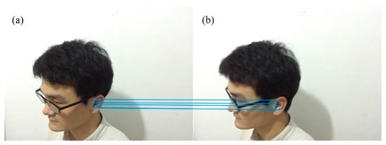
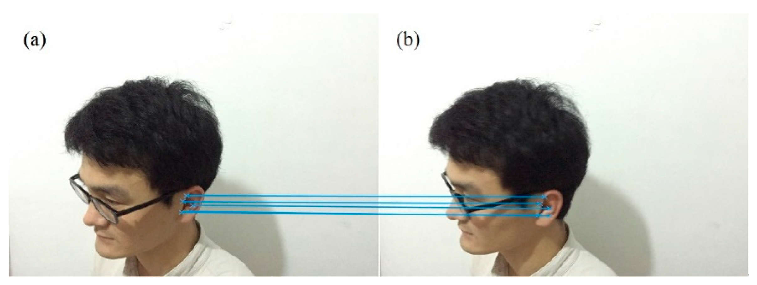
Although these three checks share partially correlated error sources and thus do not admit a simple multiplicative probability reduction, their sequential cascade effectively suppresses false matches in practice. The nearest-neighbor ratio test first removes local ambiguities in descriptor space; RANSAC subsequently enforces global epipolar geometry to discard structural outliers; and the disparity continuity check finally acts as a temporal gate to reject matches that would cause physiologically implausible depth jumps. This cascaded heuristic provides a computationally cheap yet robust validation strategy, and any residual mismatches are further mitigated by the adaptive observation noise covariance in the tracking stage. Applying the above triple-check cascade to the initial SIFT matches yields the correspondence results shown in Figure 18. The figure presents the stereo-matching results of feature points in the ear area of the passenger in normal sitting postures. Table 5 summarizes the matching results for a typical stereo pair. For the primary under laboratory conditions, the extracted SIFT keypoints in the ear region are matched with a matching rate of 100% and a matching time of 69 ms. With the progressive strategy, the matching time is reduced to approximately 45 ms while maintaining the same matching success rate for the tested cases.

Figure 18. The stereo-matching results of feature points in the area of the occupant’s ear: (a) posture I and (b) posture II.

Table 5. A summary of the obtained results of feature extraction and stereo-matching.

Parameters	Left Image	Right Image
Number of SIFT keypoints in ear region	5	5
Number of matched feature point pairs	4
Success matching rate of keypoints	100%
Matching time consumption (ms)	69 (full SIFT); 45 (stereo-matching)

5. Adaptive Kalman Filtering for Spatial Tracking

To track the ear position over consecutive frames and compensate for measurement noise, an adaptive Kalman filter is developed. The method adjusts both the process noise covariance and observation noise covariance in real time based on motion estimates and detection confidence.

5.1. Kalman Filter Formulation

The moving status of the ear feature points in each image frame can be described by their positions and velocities. For the image obtained at a moment t, assuming a feature point coordinate in the image is (x_t,y_t) and its velocities along the x and y directions are u_t and v_t, a state vector of the feature point can be defined as

$$X_t={[x_t,y_t,u_t,v_t]}^T$$

(36)

If the state vector at moment t + 1 is X_t+1, according to the Kalman filtering theory [33], the state equation of the system can be written as

X_t+1 = A_tX_t + W_t

(37)

where A_t is the state transition matrix and W_t is the Gaussian white noise matrix. If the observation vector $Z_t=\left[{\widehat{x}}_t,{\widehat{y}}_t\right]$ is the estimated feature point position at the moment t, the measurement equation of Kalman filtering is

Z_t = H_tX_t + V_t

(38)

where H_t is the system measurement matrix and V_t is the Gaussian white noise matrix of measurement.

The Kalman gain is computed as

$$K_{t+1}={\Sigma }_{t+1}^{-1}{H}_t^T{(H_t{\Sigma }_{t+1}^{-1}{H}_t^T+R_t)}^{-1}$$

(39)

where Rt is the covariance matrix. The values of the posteriori state estimation X_t+1 and the covariance matrix estimation Σ_t+1 can be updated by

$$X_{t+1}=X_{t+1}^{-1}+K_{t+1}(Z_{t+1}-H_t{X}_{t+1}^{-1})$$

(40)

$${\Sigma }_{t+1}=(I-K_{t+1}{H}_t){\Sigma }_{t+1}^{-1}$$

(41)

The spatial coordinates can be dynamically recognized by continuous posterior state estimation and new prior state prediction of the Kalman filter.

5.2. Adaptive Process Noise Covariance

Unlike the standard formulation where Q and R are fixed constants, the proposed method updates both covariances at each frame. The process noise covariance Q_t reflects the uncertainty in the motion model. The constant-velocity model fails when the occupant accelerates or decelerates. The acceleration is estimated from the observed position sequence. For each coordinate direction independently,

$${\widehat{a}}_t={\displaystyle \frac{(Z_{\mathrm{t}}-Z_{\mathrm{t}-1})-(Z_{\mathrm{t}-1}-Z_{\mathrm{t}-2})}{\Delta t^2}}$$

(42)

where Z_t, Z_t−1, and Z_t−2 are the observed positions at frames t, t − 1, and t − 2 (computed separately for x and y coordinates), and Δt is the inter-frame time interval.

To prevent high-frequency measurement noise from being misinterpreted as genuine acceleration, which would cause unnecessary inflation of Q_t, the estimated acceleration is saturated according to the physiologically feasible range of human head motion. Let A_max = 8 m/s² be the empirical upper bound for in-vehicle head movement under normal driving conditions. This value is well above the acceleration typically observed in everyday head motions (usually below 0.3 g) and even during sudden head turns (rarely exceeding 0.5 g). It is chosen to avoid noise amplification while accommodating typical occupant motions. The effective acceleration used for covariance adjustment is

$${\tilde{a}}_t=\mathit{sign}(a_t)\cdot \min (\left|a_t\right|,A_{\max })$$

(43)

This saturation ensures that the process noise adaptation remains bounded, preserving filter stability even during temporary detection jitter. The process noise covariance is then adjusted as

$$Q_t=Q_0+{\lambda }_Q\cdot \mathit{diag}({\widehat{a}}_t^2,{\widehat{a}}_t^2,{\widehat{a}}_t^2/\Delta t,{\widehat{a}}_t^2/\Delta t)$$

(44)

where Q₀ is the baseline covariance and λ_Q is a tuning parameter. When acceleration is high, Q_t increases to reflect greater model uncertainty; when motion is smooth, Q_t reverts to the baseline.

5.3. Observation Noise Covariance from Detection Confidence

The observation noise covariance R_t is mapped from the detection confidence score c_t produced by the multi-feature fusion detection in Section 3,

$$R_t=R_{\mathit{min}}+{\displaystyle \frac{R_{\mathit{max}}-R_{\mathit{min}}}{1+\exp [-\kappa \cdot (c_t-c_0)]}}$$

(45)

where R_min and R_max are the minimum and maximum covariance bounds, κ controls the steepness of the mapping, and c₀ is the confidence threshold. When detection confidence is high, R_t approaches R_min; when confidence is low, R_t increases toward R_max.

5.4. Loss-of-Track Detection and Re-Detection

The Mahalanobis distance is used as a statistical criterion for tracking loss.

$$D_M={(Z_t-H_t{X}_{t|t-1})}^{\mathrm{T}}{S}_t^{-1}(Z_t-H_t{X}_{t|t-1})$$

(46)

where $S_t=H_t{\Sigma }_{t|t-1}{H}_t^{\mathrm{T}}+R_t$ is the innovation covariance matrix. Under Gaussian assumptions, D_M follows a chi-square distribution with two degrees of freedom. If $D_M>{\chi }_{0.99}^2(2)\approx 9.21$, tracking is declared lost. Upon loss detection, a full-image re-detection procedure is triggered: the detection pipeline in Section 3 is re-executed on the entire image, and if the ear is successfully re-detected, the Kalman filter state is reinitialized with the new detection.

5.5. Experimental Verification

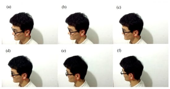
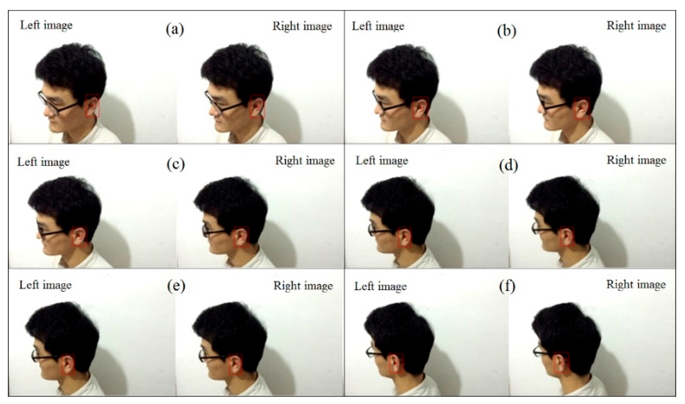
Experiments were conducted with a seated participant under laboratory conditions. The participant performed head-turning motions in a normal sitting posture and these were used for the quantitative analysis reported in Table 6. A preliminary qualitative check was also performed with a second participant having different morphological characteristics. The left and right cameras continuously captured side-view images of the occupant’s head. The detection and matching procedures from Section 3 and Section 4 are applied frame by frame, and the adaptive Kalman filter smooths the 2D image-plane positions, which are then triangulated into 3D coordinates. Figure 19 shows the results of Kalman filter tracking for different frames, indicating that the tracking algorithm can accurately track the ear area for the primary participant and the tested frames.

Table 6. The tracking spatial coordinates of the center point of the occupant’s ear in different frames.

Index #	Ear Image Coordinates (Pixels)		Tracking Spatial Coordinates (mm)	Tracking Errors (mm)
	Left Camera	Right Camera
1	(1592, 2001)	(936, 1996)	(35.5, 699.8, 403)	(−0.1, 2.8, −1.0)
2	(1613, 1980)	(941, 1972)	(35.4, 698.2, 405)	(−0.2, 3.2, 1.0)
3	(1609, 1964)	(952, 1960)	(35.1, 696.7, 404)	(−0.5, 1.7, 0.0)
4	(1591, 1942)	(937, 1937)	(34.7, 695.1, 406)	(−0.9, 0.1, 2.0)
5	(1578, 1925)	(932, 1920)	(34.1, 693.7, 408)	(−1.5, −1.3, 4.0)
6	(1616, 1903)	(967, 1896)	(33.5, 692.3, 404)	(−1.1, −2.7, 0.0)
7	(1606, 1881)	(964, 1874)	(32.6, 690.9, 405)	(−1.0, −3.1, 1.0)
8	(1616, 1664)	(958, 1641)	(31.6, 689.7, 403)	(−1.0, −4.3, −1.0)

Note: The reference coordinates were defined in the calibrated world coordinate system W as described in Section 2.1, where the origin O_W is located at the geometric center of the left camera, the Z_W axis points to the travel direction of a vehicle, and the Y_W axis is perpendicular to the horizontal plane. The per-axis error is $e_i=q_i-{\widehat{q}}_i$, and the 3D Euclidean error is $e_{3D}=\sqrt{e_x^2+e_y^2+e_z^2}$. These results are representative samples from one seated participant under laboratory conditions.

Figure 19. The results of Kalman filter tracking: (a) 20th, (b) 40th, (c) 60th, (d) 80th, (e) 100th and (f) 120th frames.

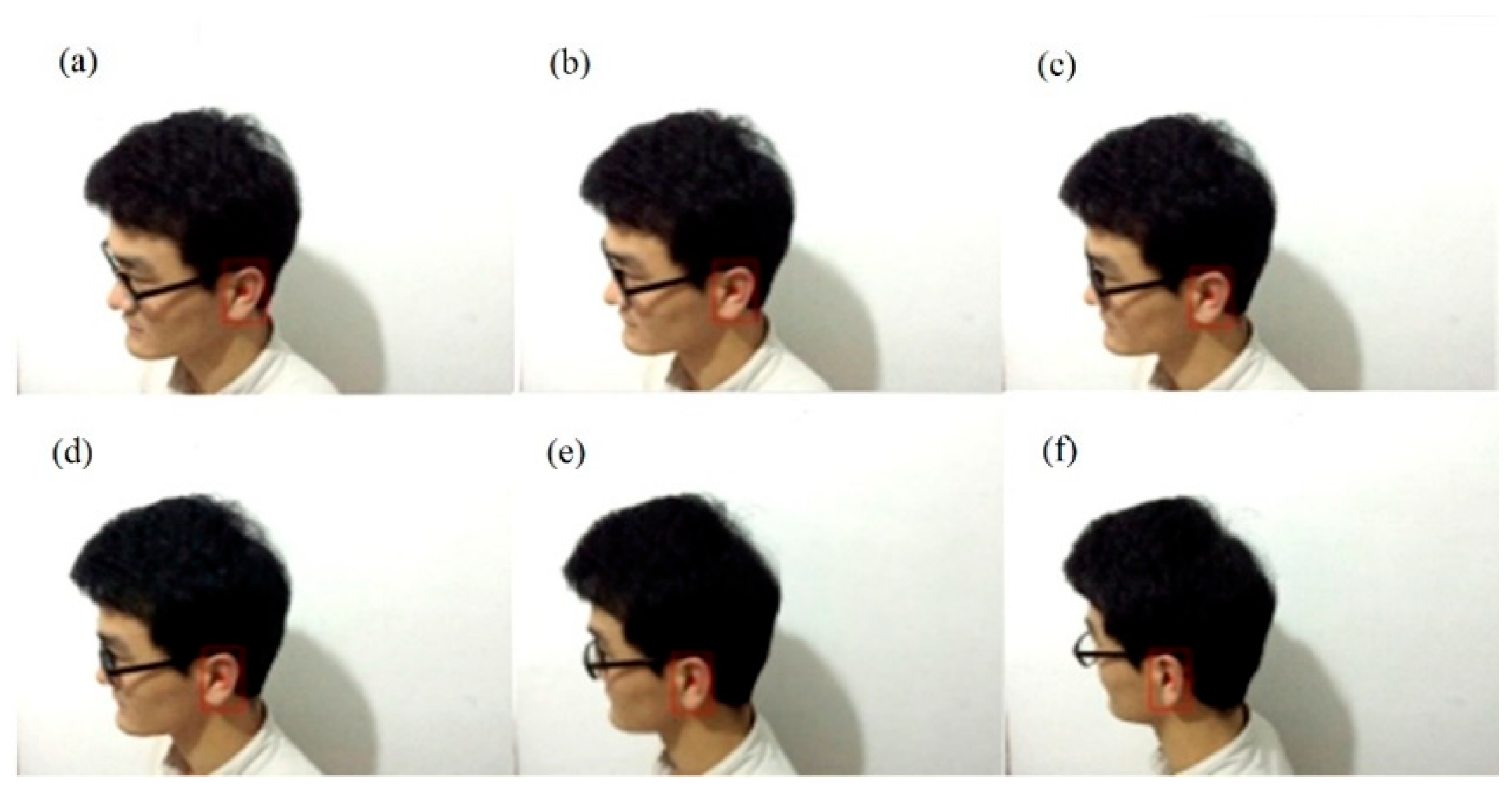
Figure 20 shows the detected results of the occupant’s ear for frames 20, 40, 60, 80, 100, and 120. The red bounding box marks the ear region and the red dot marks the region center.

Figure 20. The detected results of the occupant’s ear: (a) 20th, (b) 40th, (c) 60th, (d) 80th, (e) 100th and (f) 120th frames.

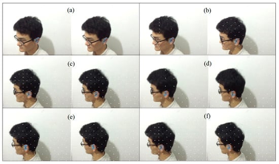
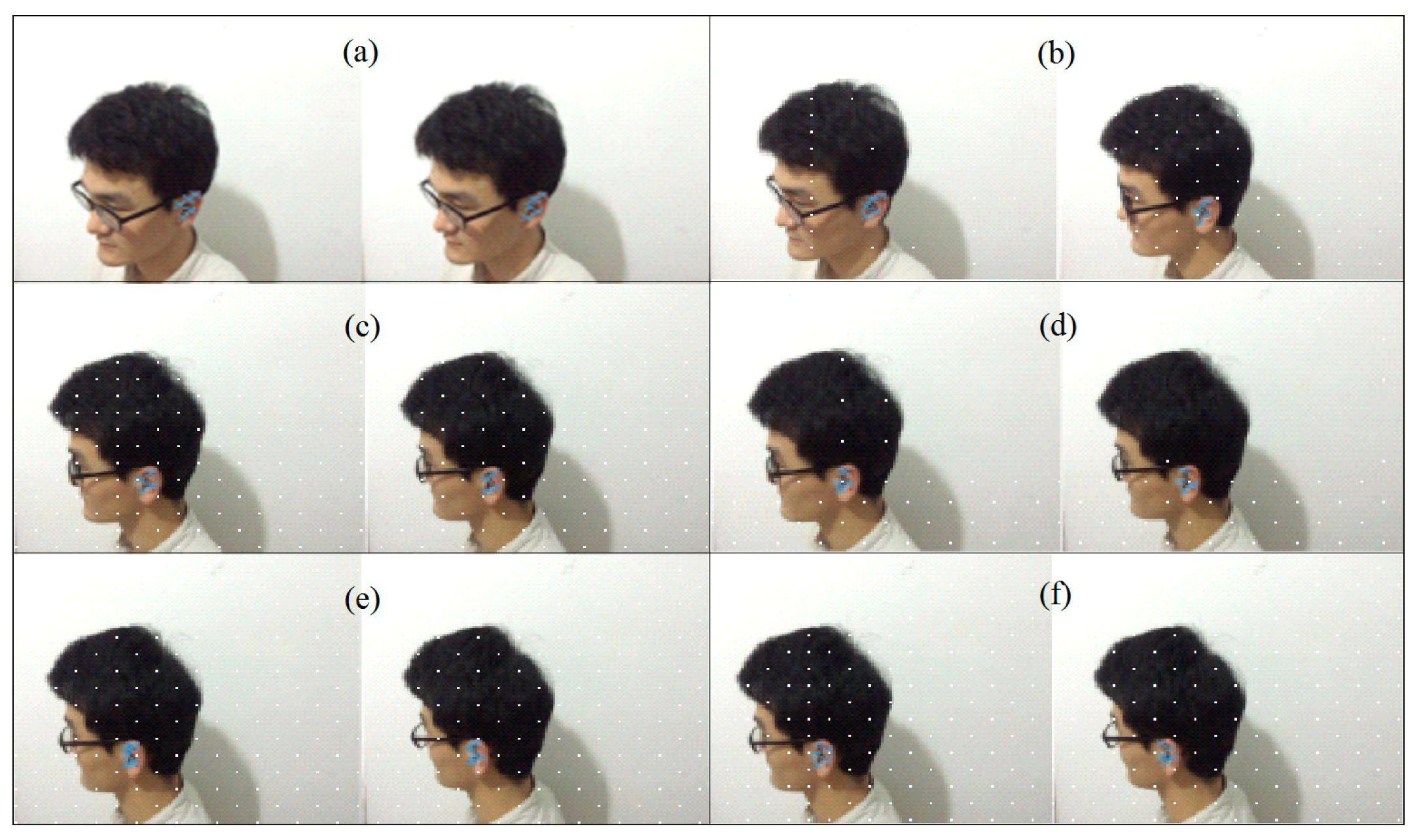
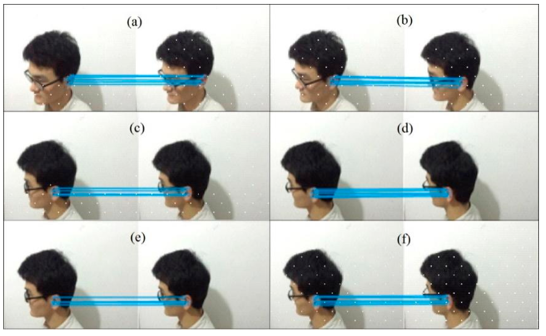
Figure 21 shows the extracted features of the occupant’s ear, and Figure 22 shows the stereo-matching results of feature points. The binocular stereovision system successfully extracts feature points from both views, as shown in Figure 21, and the stereo correspondences are established for the tested frames in Figure 22.

Figure 21. The extracted features of an occupant’s ear: (a) 20th, (b) 40th, (c) 60th, (d) 80th, (e) 100th and (f) 120th frames.

Figure 22. The stereo-matching results of feature points: (a) 20th, (b) 40th, (c) 60th, (d) 80th, (e) 100th and (f) 120th frames.

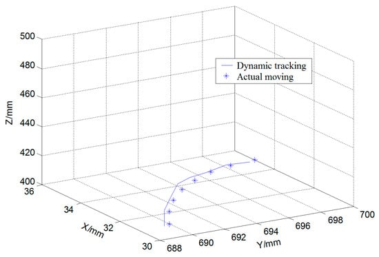
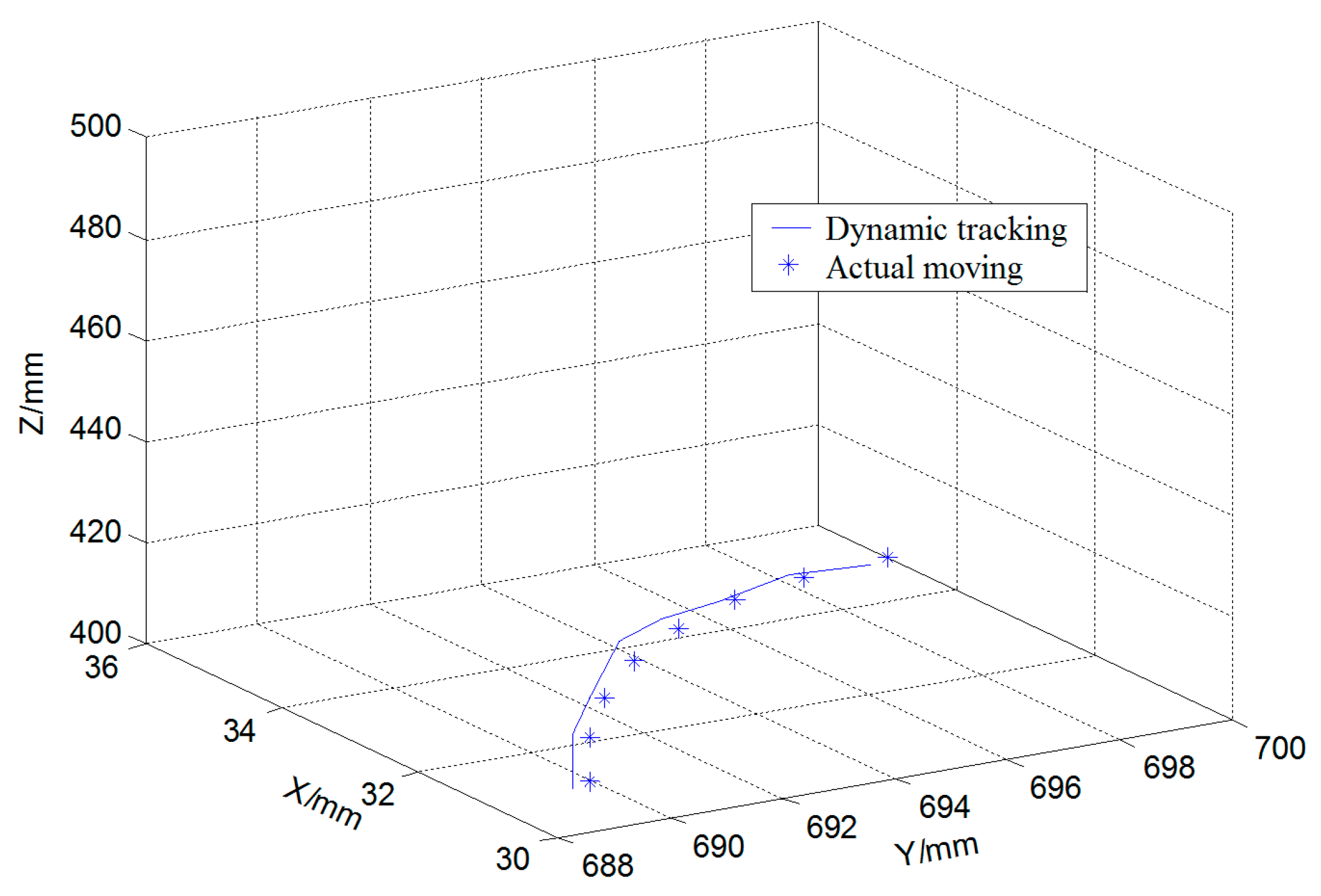
Table 6 presents the tracking results for eight representative frames selected from the evaluated sequence of 120 frames. The error definition and the source of the reference coordinates are given in the caption for Table 6. The per-axis errors are within ±4.5 mm and the maximum 3D Euclidean error is 4.52 mm among the reported representative samples. Figure 23 compares the tracked trajectory with the reference ear motion defined in the calibrated world coordinate system, showing close agreement for the tested frames.

Figure 23. A comparison of the moving tracks of the center point of the occupant’s ear.

To validate the adaptive mechanism, a comparative experiment is conducted under two conditions in the laboratory. Condition A uses the standard Kalman filter with fixed process noise covariance Q and measurement noise covariance R as the baseline. Condition B employs the proposed adaptive Kalman filter with time-varying Q_t and R_t. During the sudden head turn (frames 80–100), Condition B maintains the tracking error within approximately 5 mm, while Condition A exhibits a maximum error exceeding 15 mm. Condition B also maintains continuous tracking throughout the turn, whereas Condition A shows intermittent tracking discontinuity. Under the tested artificial illumination change (frames 50–70), the detection confidence drops for several frames; the adaptive mechanism increases R_t accordingly and maintains tracking, whereas the fixed-R filter diverges and fails to recover. These results under the tested laboratory conditions indicate improved robustness of the adaptive Kalman filter under sudden motion and illumination variation. The re-detection mechanism was triggered when the Mahalanobis distance exceeded the threshold; recovery was observed in the tested cases.

5.6. Vehicle-Specific Factors and Future Extensions

The present work establishes the core detection–matching–tracking pipeline under simplified in-vehicle conditions. The framework is a laboratory proof-of-concept for future in-vehicle acoustic applications. To move toward real-vehicle deployment, several vehicle-specific factors need to be considered. Vehicle vibration from road or engine sources may cause relative motion between the cameras and the occupant, leading to image blur, feature-point drift, and disparity jitter; the adaptive Kalman filter and re-detection mechanism provide partial compensation. Natural illumination through windows, including strong backlight and rapidly changing shadows, may affect skin-color segmentation and SIFT feature stability; the online skin-color model and confidence-driven observation noise adjustment are designed to mitigate these variations. Seat-position changes alter the camera-to-ear distance and viewing angle, affecting disparity, depth resolution, and the region of interest; the Kalman-predicted search window can partially accommodate such changes. Partial occlusions by hair, eyeglasses, masks, or hats may reduce valid SIFT keypoints and cause tracking loss; the cascaded detection and re-detection scheme may partially compensate. Realistic occupant motion, such as sudden head turns, fore–aft movements, and nodding, may introduce motion blur and challenge the constant-velocity assumption of the Kalman filter; the adaptive process noise covariance is intended to address this issue. These mechanisms form a natural basis for future extensions.

The illumination test was conducted under laboratory ceiling illumination, with one artificial illumination change introduced between frames 50 and 70. Quantitative detection confidence, localization error, tracking continuity, and re-detection frequency under illumination variation were not logged. Systematic illumination testing under a wider range of conditions remains for future work. Moreover, the reported 45 ms refers only to the stereo-matching stage, not to the full detection, feature extraction, matching, tracking, triangulation, and re-detection pipeline. The accuracy requirement reported in [4] provides a useful reference for the intended acoustic application. Full-pipeline timing was not recorded and will be measured on an embedded platform in future work. In addition, the processor, memory, operating environment, implementation language, and GPU acceleration were not recorded, so full-pipeline frame rate cannot be inferred from the 45 ms value. The SIFT contrast threshold of 0.03 was not optimized in the present study: it is the value of Lowe’s original formulation [32]. The acceleration saturation limit of 8 m/s² was chosen empirically. Their values should be examined through sensitivity analysis. The present validation is limited to one seated participant. The method relies partly on skin-color, geometric, and contour priors, which may vary across different skin tones, ear geometries, hairstyles, ages, and genders. The online skin-color model and contour matching have been tested on two participants with different morphological characteristics, and the preliminary results are promising. However, the sample size remains small, and the second participant was used only for qualitative verification. Therefore, the present results should be understood as preliminary evidence of feasibility. Further validation is needed to establish robustness across participants and practical applicability in vehicles.

6. Conclusions

This paper presents a dynamic recognition and tracking method for spatial coordinates of the occupant’s ear based on a binocular stereovision model. A binocular stereovision system and the relationships among its four coordinate systems are established. The binocular stereovision system is calibrated by using the two-step RAC method. The error analysis of reconstruction experiments indicates that this calibration method is computationally efficient and provides reasonable reprojection accuracy under laboratory conditions.

Three specific improvements are made to mitigate the limitations of existing methods. In the detection stage, a coarse-to-fine cascade strategy is developed that integrates skin-color prior, geometric constraints, and contour matching. The skin-color model is updated online with a forgetting factor to adapt to illumination variations in the tested laboratory setting, and a confidence score is output for each detection. In the matching stage, feature points are ranked by importance using a saliency-guided heuristic metric, and only the top-ranked ones are retained for matching. The search window is dynamically constrained by the Kalman-predicted position, and a triple-check mechanism is applied to improve matching quality. In the tracking stage, an adaptive Kalman filter is used where the process noise covariance is adjusted based on acceleration estimates and the observation noise covariance adapts to detection confidence. A Mahalanobis distance-based criterion triggers full-image re-detection upon tracking loss.

A preliminary qualitative check with a second participant also showed promising feasibility. The proposed method tracked the occupant’s ear spatial coordinates. The maximum 3D Euclidean error was 4.52 mm for representative frames. Preliminary comparisons suggest improved reliability under the tested laboratory conditions for the adaptive Kalman filter under sudden head motion and illumination variation. General robustness across participants and illumination conditions or vehicle-specific conditions is not claimed. The re-detection mechanism recovered tracking in the tested cases. Unlike learning-based paradigms, the method offers a deterministic pipeline with bounded heuristic parameters. This suggests potential for future latency-sensitive in-vehicle acoustic applications such as active noise control. In such applications, delay jitter and black-box behavior are undesirable.

Nevertheless, this study is a laboratory proof-of-concept. These limitations and the expected influence of vehicle-specific factors have been further discussed. Future work will address multi-subject validation, controlled illumination, occlusion evaluation, full-pipeline timing, sensitivity analysis of heuristic parameters, and real-vehicle validation.

References

- Oh, J.Y.; Kim, J.Y.; Oh, C.S.; Doe, J.H.; Kang, Y.J. Head-tracking active road noise control by real-time path adaptation using neural networks. Mech. Syst. Signal Process. 2026, 250, 114106. [Google Scholar] [CrossRef] [Scilit]
- Zhang, W.; Zou, Y.; Wang, Y. Ear tracking via Siamese hierarchical refinement network for local active noise control. J. Real-Time Image Process. 2021, 18, 635–646. [Google Scholar] [CrossRef] [Scilit]
- Tseng, W.K. Local active noise control using a novel method of designing quiet zones. Control Eng. Pract. 2011, 19, 1450–1458. [Google Scholar] [CrossRef] [Scilit]
- Jiang, H.; Chen, H.; Tao, J.; Zou, H.; Qiu, X. Accuracy requirements of ear-positioning for active control of road noise in a car. Appl. Acoust. 2024, 225, 110164. [Google Scholar] [CrossRef] [Scilit]
- Zhang, C. Monocular 3d binaural localization and dynamic tracking for ear-side active noise control in vehicle cabins. World J. Eng. Res. 2026, 4, 52–61. [Google Scholar] [CrossRef] [Scilit]
- Xu, Q.; Wang, S.; Tao, J.; Zou, H.; Qiu, X. Creating personal sound zones in car cabins with active noise control. Appl. Acoust. 2025, 235, 110670. [Google Scholar] [CrossRef] [Scilit]
- Li, X.; Wu, X.; Huang, J.; Feng, Q. Sound zoning modulation within non-enclosed vehicular cavities: Targeted compensation for dynamic reverberation and wind-induced noise. Eng. Appl. Artif. Intell. 2026, 176, 114764. [Google Scholar] [CrossRef] [Scilit]
- Qiao, Y.; Luo, J.; Choueiri, E.Y. Spatial sampling of binaural room transfer functions for head-tracked personal sound zones. AES J. Audio Eng. Soc. 2024, 72, 455–466. [Google Scholar] [CrossRef] [Scilit]
- Shivappa, S.T.; Rao, B.D.; Trivedi, M.M. Role of head pose estimation in speech acquisition from distant microphones. In 2009 IEEE International Conference on Acoustics, Speech and Signal Processing; IEEE: New York, NY, USA, 2009; pp. 3557–3560. [Google Scholar]
- Al-Mafrachi, R.; Gimm, M.; Schmidt, G. Acoustic estimation of the head orientation for in-car communication systems. Fortschritte Akust. DAGA 2018, 2018, 1780–1783. [Google Scholar]
- Alefs, B.; Clabian, M.; Bischof, H.; Kropatsch, W.; Khairallah, F. Robust occupancy detection from stereo images. In Proceedings of the 7th International IEEE Conference on Intelligent Transportation Systems (IEEE Cat. No. 04TH8749); IEEE: New York, NY, USA, 2004; pp. 1–6. [Google Scholar]
- Ziraknejad, N.; Lawrence, P.D.; Romilly, D.P. Vehicle occupant head position quantification using an array of capacitive proximity sensors. IEEE Trans. Veh. Technol. 2014, 64, 2274–2287. [Google Scholar] [CrossRef] [Scilit]
- Zhang, M.; Zhang, F. A driver fatigue detection method based on eye aspect ratio compensated by head pose estimation. In 2023 8th International Conference on Signal and Image Processing (ICSIP); IEEE: New York, NY, USA, 2023; pp. 161–165. [Google Scholar]
- Preu, V.; Pauer, D.; Putter, R.; Hecker, P. ICF-Fusion: Multimodal In-Cabin Sensor Fusion for Adaptive Restraint Systems. Vehicles 2026, 8, 182. [Google Scholar] [CrossRef] [Scilit]
- Jain, D.; Miller, J. Towards Audio Personalization for Accessible Digital Media. In Proceedings of the 27th International Conference on Multimodal Interaction, Canberra, Australia, 13–17 October 2025; pp. 381–386. [Google Scholar]
- Inan, T.; Kacar, U. Ear semantic segmentation in natural images with Tversky loss function supported DeepLabv3+ convolutional neural network. Balk. J. Electr. Comput. Eng. 2022, 10, 337–346. [Google Scholar] [CrossRef] [Scilit]
- Prakash, S.; Jayaraman, U.; Gupta, P. A skin-color and template based technique for automatic ear detection. In 2009 Seventh International Conference on Advances in Pattern Recognition; IEEE: New York, NY, USA, 2009; pp. 213–216. [Google Scholar]
- Hemamalini, V.; Annapurani, K.; Saha, P.; Batra, K.; Chatterjee, J. Feature Extraction of the Human Ear Based on Enhanced Active Contour Method. Procedia Comput. Sci. 2024, 235, 2897–2908. [Google Scholar] [CrossRef] [Scilit]
- Liu, D.K.; Liu, H. Combining Skin Color Model and Multi-template Matching for Enhancing Adaboost Ear Detection. J. Southwest Univ. Sci. Technol. 2010, 25, 91–95. [Google Scholar]
- Wen, B.; Dewan, S.; Birchfield, S. Fast-FoundationStereo: Real-time zero-shot stereo matching. In Proceedings of the IEEE/CVF Conference on Computer Vision and Pattern Recognition, Denver, CO, USA, 2–6 June 2026; pp. 7513–7524. [Google Scholar]
- Tsai, S.E.; Hsieh, C.H. A real-time collision warning system for autonomous vehicles based on YOLOv8n and SGBM stereo vision. Electronics 2025, 14, 4275. [Google Scholar] [CrossRef] [Scilit]
- Yang, X.; Zhong, J.; Lin, K.; Wu, J.; Chen, J.; Si, H. Research progress on binocular stereo vision technology and its applications in smart agriculture. Trans. Chin. Soc. Agric. Eng. 2025, 41, 27–39. [Google Scholar]
- Han, F.; Liu, J.; Zhang, G.; Yu, T.; Zhang, X.; Qian, J. A survey of ranging algorithms based on binocular stereo vision. In 2024 China Automation Congress (CAC); IEEE: New York, NY, USA, 2024; pp. 2388–2393. [Google Scholar]
- Niu, Y.; Gao, L.; Yu, W.; Huang, Z.; Liu, H. A review of binocular vision stereo matching algorithms. J. Eur. Opt. Soc.-Rapid Publ. 2026, 22, 60. [Google Scholar] [CrossRef] [Scilit]
- Song, D.; Jiang, Q.; Sun, W.; Yao, L. A survey: Stereo based navigation for mobile binocular robots. In Proceedings of the 1st International Conference on Robot Intelligence Technology and Applications; Springer: Berlin/Heidelberg, Germany, 2013; pp. 1035–1046. [Google Scholar]
- Rodríguez-Martínez, E.A.; Flores-Fuentes, W.; Achakir, F.; Sergiyenko, O.; Murrieta-Rico, F.N. Vision-based navigation and perception for autonomous robots: Sensors, SLAM, control strategies, and cross-domain applications—A review. Eng 2025, 6, 153. [Google Scholar] [CrossRef] [Scilit]
- Bruno, D.R.; Berri, R.A.; Barbosa, F.M.; Osório, F.S. CARINA Project: Visual perception systems applied for autonomous vehicles and advanced driver assistance systems (ADAS). IEEE Access 2023, 11, 69720–69749. [Google Scholar] [CrossRef] [Scilit]
- Jing, J.; Mao, Y.; Mikolajczyk, K. Match-stereo-videos: Bidirectional alignment for consistent dynamic stereo matching. In European Conference on Computer Vision; Springer Nature: Cham, Switzerland, 2024; pp. 415–432. [Google Scholar]
- Li, J.; Xu, X.; Jiang, Z.; Jiang, B. Adaptive Kalman filter for real-time visual object tracking based on autocovariance least square estimation. Appl. Sci. 2024, 14, 1045. [Google Scholar] [CrossRef] [Scilit]
- Liu, X.; Lu, R. Calibration of a stereo microscope based on non-coplanar feature points with iteratively weighted radial alignment constraint. Opt. Lasers Eng. 2020, 127, 105977. [Google Scholar] [CrossRef] [Scilit]
- Lee, J.S.; Jeong, Y.H. CCD camera calibrations and projection error analysis. In Proceedings KORUS 2000. The 4th Korea-Russia International Symposium on Science and Technology.; IEEE: New York, NY, USA, 2000; Volume 2, pp. 50–55. [Google Scholar]
- Lowe, D.G. Distinctive image features from scale-invariant keypoints. Int. J. Comput. Vis. 2004, 60, 91–110. [Google Scholar] [CrossRef] [Scilit]
- Pogorelyuk, L.; Rowley, C.W.; Kasdin, N.J. An efficient approximation of the Kalman filter for multiple systems coupled via low-dimensional stochastic input. Automatica 2020, 117, 108972. [Google Scholar] [CrossRef] [Scilit]
Disclaimer/Publisher’s Note: The statements, opinions and data contained in all publications are solely those of the individual author(s) and contributor(s) and not of MDPI and/or the editor(s). MDPI and/or the editor(s) disclaim responsibility for any injury to people or property resulting from any ideas, methods, instructions or products referred to in the content. |
© 2026 by the authors. Published by MDPI on behalf of the World Electric Vehicle Association. Licensee MDPI, Basel, Switzerland. This article is an open access article distributed under the terms and conditions of the Creative Commons Attribution (CC BY) license.