


Highlights
What are the main findings?
- Bidirectional magneto-thermal coupling captures the feedback between winding temperature, copper resistivity, and copper loss.
- Experiments validate the baseline model’s predictions of end-winding temperature and coolant pressure drop.
What are the implications of the main findings?
- Universal Kriging surrogate modeling and the non-dominated sorting genetic algorithm II (NSGA-II) provide an approach for balancing maximum motor temperature and coolant pressure drop.
- Independent computational fluid dynamics (CFD) calculations predict that the selected compromise channel reduces the pressure drop by 32.45% and the maximum motor temperature by 3.38 K.
Abstract
Permanent magnet synchronous motors (PMSMs) are increasingly used in electric vehicles, where rising power density and compact packaging impose greater demands on motor thermal management. However, cooling-channel design involves a coupled trade-off between heat removal and hydraulic resistance, while temperature-dependent electromagnetic losses are often not fully considered in optimization studies. To address this issue, this study investigates the multi-objective optimization and verification of a helical cooling channel for a liquid-cooled PMSM based on bidirectional magneto-thermal coupling. A three-dimensional transient electromagnetic model was coupled with a conjugate heat-transfer model to account for the feedback between winding temperature, copper resistivity, electromagnetic loss, and motor temperature. An experimental temperature-rise test bench was established for model validation, and an optimal Latin hypercube design, Universal Kriging surrogate models, and the non-dominated sorting genetic algorithm II (NSGA-II) were integrated in Isight (v2022, Dassault Systèmes, Vélizy-Villacoublay, France) to optimize the channel height, width, and fillet radius with the maximum motor temperature and coolant pressure drop as the objectives. Results show that the numerical model reproduced the measured thermal-hydraulic responses over the investigated coolant-flow-rate range, with maximum deviations of 1.16% for the end-winding temperature and 5.54% for the coolant pressure drop. Under the investigated peak-power condition, the total electromagnetic loss was 3864 W, of which the stator winding and stator core accounted for 66.2% and 30.5%, respectively, confirming that they are the dominant heat sources. The Universal Kriging model achieved training coefficients of determination of 0.97 and 0.98, with corresponding 10-fold cross-validated values of 0.953 and 0.968, for the maximum motor temperature and coolant pressure drop, respectively, and was therefore selected for NSGA-II optimization. For the selected compromise solution, the independently calculated pressure drop decreased from 12,312.97 to 8318.54 Pa, corresponding to a reduction of 32.45%, while the maximum motor temperature decreased from approximately 375.18 to 371.80 K, or by 3.38 K. The deviations between the surrogate predictions and independent computational fluid dynamics (CFD) results were 1.47% for pressure drop and 0.20% for maximum temperature. The proposed framework provides a physically consistent and experimentally supported method for the thermal-hydraulic design of PMSM cooling channels and offers a basis for further optimization of high-power-density motor thermal management systems.
1. Introduction
Permanent magnet synchronous motors (PMSMs) are widely used as drive motors in new energy vehicles because of their high power density, high efficiency, and broad speed regulation capability [1]. As the demand for higher power density, compact structure, and wider operating range continues to grow, the thermal load of PMSMs has increased accordingly. If the heat generated during operation cannot be removed effectively, the temperature of the windings and permanent magnets may rise beyond the allowable limit, which can accelerate insulation aging, induce irreversible demagnetization, and reduce motor efficiency and reliability. These thermal issues may also affect the safety and durability of the vehicle. Therefore, an effective cooling strategy is essential to ensure the stable operation of PMSMs [2,3].
Among the available thermal management methods, liquid cooling has become one of the most commonly adopted solutions for PMSMs because of its relatively high heat transfer capability and good temperature uniformity. However, the cooling performance of a PMSM is strongly influenced by the geometry of the cooling channel, while the corresponding flow resistance also changes with channel design. Recent studies have shown that cooling-jacket geometry, flow-path configuration, and local heat-transfer conditions jointly affect the thermal and hydraulic performance of electric machines [4,5,6]. This makes cooling channel design a typical multi-objective problem, in which thermal performance and hydraulic performance must be considered simultaneously. In addition, the heat generation of the motor depends on operating conditions and material properties, which are both affected by temperature. Comparative studies of stator cooling jackets have likewise demonstrated that channel configuration affects both motor temperature and cooling-system performance [7]. Therefore, magneto-thermal coupling analysis is necessary to obtain a more accurate description of loss distribution and temperature rise, and it provides a reliable basis for the subsequent optimization of cooling channel structures. The importance of accurately representing the thermal load is particularly evident in high-power-density machines, where copper and core losses can contribute substantially to the overall temperature rise [8,9,10,11].
Liquid cooling is widely adopted in PMSMs because of its relatively high heat removal capability and good temperature uniformity. In practical applications, however, the thermal performance of a liquid-cooled motor is closely related to the geometry of the cooling channels, which also determines the pressure drop and pumping demand of the system. This trade-off has been reported in recent cooling-system studies, in which enhanced heat removal must be balanced against increased flow resistance and pumping requirements [12,13]. As a result, the design of cooling channels is not a single thermal problem but a coupled thermal-hydraulic problem that requires a balance between heat dissipation and flow resistance.
In addition, the loss distribution of a PMSM is strongly temperature dependent. As the operating temperature rises, the resistivity of the winding conductors increases, and the magnetic properties of the permanent magnets, as well as those of the iron core to a lesser extent, may also change. These variations modify the electromagnetic losses during operation and, in turn, affect the temperature field of the motor. This mutual interaction between loss generation and heat transfer makes magneto-thermal coupling analysis necessary for a more accurate evaluation of motor thermal behavior. It also provides a sound basis for the multi-objective optimization and verification of cooling channel structures [14,15].
In related studies, Jeon et al. [3] investigated the influence of different water jacket configurations on the cooling performance of PMSMs through electromagnetic-thermal-fluid coupling analysis and design of experiments. Computationally efficient cooling-jacket models have also been developed to facilitate repeated thermal analyses of electric machines [15]. Other studies have investigated local cooling strategies, including rotor air-cooling enhancement and direct end-winding cooling, highlighting the importance of matching the cooling method with the dominant heat-transfer paths [4,16]. Their results showed a clear relationship between channel geometry, heat dissipation capability, and flow resistance, which provides useful guidance for parameter selection in multi-objective optimization. Similar relationships between cooling-channel geometry, heat removal, and pressure loss have been reported for PMSM cooling systems used in transportation applications [17]. Tong et al. [18] developed a three-dimensional electromagnetic-thermal bidirectional coupling model for high-speed PMSMs and analyzed the loss and temperature-rise characteristics in detail. Their work established a solid basis for the accurate prediction of electromagnetic losses and thermal behavior in optimization studies.
Zheng et al. [19] proposed an optimization method for parallel air-cooled channels of a magnetic levitation permanent magnet motor, aiming to improve flow distribution and reduce inlet static pressure. Recent studies have further applied surrogate-assisted optimization to motor cooling systems to reduce the computational cost of repeated numerical evaluations while considering multiple performance objectives [12]. By combining design of experiments, sensitivity analysis, a radial basis function neural network surrogate model, and a multi-island genetic algorithm in Isight, they completed the optimization process and demonstrated an effective strategy for multi-objective thermal design. Similarly, Chen et al. [20] employed a particle-swarm-optimization-based backpropagation neural network (PSO–BPNN) to construct a surrogate model and then used the non-dominated sorting genetic algorithm II (NSGA-II) to achieve the coordinated optimization of temperature rise and pressure drop. Cooling-system optimization studies have also examined asymmetric configurations and coupled thermal–hydraulic responses, but temperature-dependent electromagnetic loss feedback has not always been included in the optimization loop [5,12]. Their study formed a workflow integrating experimental design, surrogate modeling, and algorithm-based optimization, offering useful reference for motor thermal management. These studies indicate that surrogate-assisted multi-objective optimization has broad potential in the thermal design of motor cooling systems. However, for PMSMs, there is still a need for a more complete framework that combines magneto-thermal coupling analysis, cooling channel optimization, and experimental verification.
Despite the progress made in the thermal analysis and design of PMSM cooling systems, an integrated framework that combines magneto-thermal coupling analysis, multi-objective optimization, and verification of cooling channel structures is still limited. In particular, the nonlinear coupling among channel geometry, heat dissipation performance, flow resistance, and pumping demand has not been characterized sufficiently for design-oriented optimization. To address this gap, the present study establishes a bidirectional magneto-thermal coupling model to capture the interaction between electromagnetic losses and temperature rise under operating conditions. Based on this model, the cooling-channel geometry is optimized in Isight by minimizing the maximum motor temperature and coolant pressure drop, while the key structural parameters are treated as design variables. Finally, the optimized channel scheme is verified through simulation and experimental comparison, providing a more reliable basis for the design and evaluation of PMSM cooling channels.
2. Materials and Methods
2.1. Magneto-Thermal Coupling Theory and Calculation Procedure
Electromagnetic losses constitute the main heat sources in a permanent magnet synchronous motor (PMSM), while the resulting temperature rise affects the temperature-dependent properties of the motor materials. In particular, an increase in winding temperature raises the electrical resistivity of copper and consequently increases the winding loss. The modified loss distribution, in turn, affects the motor temperature field. Therefore, a one-way thermal analysis based on electromagnetic losses calculated at a fixed reference temperature may not fully represent the interaction between loss generation and temperature rise. To account for this feedback, a bidirectional magneto-thermal coupling procedure was established for the operating condition considered in this study. The calculation procedure is shown in Figure 1.
Figure 1.
Flowchart of the bidirectional magneto-thermal coupling procedure.
At the beginning of the coupling calculation, the material properties are initialized, and a three-dimensional electromagnetic analysis is performed to determine the losses in the stator core, rotor core, windings, and permanent magnets. The loss of each component is divided by its corresponding volume and converted into a volumetric heat-generation rate. The resulting heat-generation rates are then transferred to the fluid-solid conjugate heat-transfer model as heat-source inputs. Under the specified operating and cooling boundary conditions, the thermal-fluid model simultaneously solves the coolant flow field and the temperature distributions in the solid components and fluid domain.
After each thermal-fluid calculation, the calculated winding temperature is transferred back to the electromagnetic model and used to update the electrical resistivity of the copper windings. The electromagnetic losses are then recalculated using the updated material property and transferred again to the thermal-fluid model. According to the assumptions described in Section 2.2, the temperature dependence of the iron-core and permanent-magnet losses is neglected because their variations have a limited influence on the total heat generation under the investigated operating condition. Therefore, the feedback process considered in the present coupling model mainly accounts for the effect of winding temperature on copper resistivity and winding loss.
During the preliminary bidirectional coupling calculations, the electromagnetic and thermal-fluid analyses were terminated when the relative change in the maximum motor temperature between two consecutive iterations was less than 5%. This criterion was adopted as a practical preliminary stopping condition to balance convergence monitoring and the computational cost of repeated electromagnetic and thermal-fluid analyses. However, because the temperature improvement obtained after optimization was 3.38 K, the 5% criterion was not used as the sole basis for the final assessment of the coupled solution.
A convergence-sensitivity analysis was therefore conducted using a stricter criterion. In the revised calculation, the relative changes in both the maximum motor temperature and the total electromagnetic loss between two consecutive iterations were required to be less than 1%. For the baseline motor and baseline cooling-channel configuration under the selected peak-power operating condition, the bidirectional coupling calculation converged after six iterations. Between the final two iterations, the maximum motor temperature changed from 375.17 to 375.16 K, corresponding to an absolute change of 0.01 K and a relative change of 0.0027%. During the same iteration interval, the total electromagnetic loss changed from 3864.10 to 3864.00 W, corresponding to a change of 0.10 W and a relative change of 0.0026%. The winding copper loss changed from 2558.10 to 2558.00 W, corresponding to a change of 0.10 W and a relative change of 0.0039%.
To evaluate the influence of the coupling convergence criterion on the reported optimization result, the converged loss distributions obtained using the 5% and 1% criteria were separately transferred as fixed volumetric heat sources to the thermal-fluid models of the baseline and selected optimized channel configurations. Under the 5% criterion, the maximum temperatures of the baseline and selected optimized configurations were 375.18 and 371.80 K, respectively, corresponding to a temperature improvement of 3.38 K. Under the stricter 1% criterion, the corresponding maximum temperatures were 375.16 and 371.79 K, respectively, corresponding to a temperature improvement of 3.37 K. The difference between the two temperature improvements was only 0.01 K, which is much smaller than the reported temperature improvement of 3.38 K. These results indicate that the reported thermal improvement and the selection of the optimized channel are not significantly affected by the coupling convergence criterion.
For the subsequent cooling-channel optimization, the bidirectional electromagnetic–thermal coupling procedure was performed only for the baseline motor and baseline cooling-channel configuration under the selected peak-power operating condition. The loss distribution obtained using the stricter 1% criterion was retained as the final electromagnetic heat-source input and assigned to the winding, stator core, rotor core, and permanent-magnet domains as fixed volumetric heat sources. The bidirectional electromagnetic–thermal coupling was not repeated for every candidate channel geometry. This treatment was adopted because the electromagnetic geometry, operating current, and rotational speed remained unchanged during the optimization, whereas only the housing-channel geometry was varied. It allowed the thermal–hydraulic effects of different channel designs to be compared under a common electromagnetic heat-source condition.
The candidate-specific change in winding temperature and its associated feedback on copper resistivity and winding loss were therefore not included during the optimization. Because the temperature dependence of the iron-core and permanent-magnet losses was neglected according to the assumptions in Section 2.2, the main omitted feedback was the change in winding loss caused by the different winding temperatures of the candidate designs. Consequently, the optimized results represent the thermal and hydraulic performance of the channel designs under the prescribed common heat-source condition. If different channel designs produce substantially different winding temperatures, a fully coupled recalculation may lead to different winding losses and may affect the predicted maximum temperature and the resulting thermal–hydraulic trade-off.
The maximum motor temperature obtained for each channel design was used to evaluate its thermal performance, whereas the coolant pressure drop was used to characterize its hydraulic resistance and associated pumping demand. In this manner, the converged magneto-thermal analysis provided a consistent electromagnetic heat-source basis for the subsequent thermal-fluid simulations, surrogate-model construction, and multi-objective optimization of the cooling-channel geometry.
2.2. Electromagnetic Loss Model of the PMSM
Accurate determination of electromagnetic losses is essential for predicting the temperature distribution of a PMSM, because these losses provide the heat-source inputs for the subsequent thermal-fluid analysis. In the motor considered in this study, the stator windings, laminated cores, and permanent magnets produce losses through different mechanisms and exhibit different spatial distributions. A three-dimensional transient electromagnetic model was therefore established to account for the actual motor geometry, the internal V-shaped arrangement of the permanent magnets, and the axial non-uniformity of the electromagnetic field. Compared with a two-dimensional model, the three-dimensional formulation can represent end effects and axial current paths more directly, which is particularly relevant to the evaluation of eddy-current losses in the rotor and permanent magnets.
The electromagnetic field was solved under the specified peak-power operating condition using the magnetic vector potential–electric scalar potential formulation. The rotational speed was n = 4500 rpm, the phase current was I = 150 A in root-mean-square value, the current phase angle was β = 25°, and the electromagnetic frequency was fe = 300 Hz. The corresponding electromagnetic torque was T = 170 Nm, giving a mechanical output power of approximately 80 kW. For the eight-pole machine, the electrical frequency was calculated from fe = pn/60, where p = 4 is the number of pole pairs. Here, β denotes the current phase angle according to the reference-axis convention adopted in the electromagnetic model. Under the magneto-quasistatic assumption, displacement currents were neglected because their contribution was negligible at the operating frequencies considered. The governing equations are expressed as follows:
where A, ϕ, and Ja are the vector magnetic potential, scalar electric potential and armature current density, respectively; M is the permanent magnet magnetization intensity; μ and σ are the permeability and conductivity, respectively.
The material properties used in the electromagnetic model influence both the field distribution and the calculated losses. In particular, the magnetic characteristics of the laminated cores affect the local flux-density distribution and iron loss, whereas the electrical conductivities of the windings and permanent magnets determine the corresponding resistive and eddy-current losses. Since the electrical resistivity of copper varies appreciably with temperature, the winding loss is updated during the bidirectional magneto-thermal coupling procedure described in Section 2.1. The losses obtained after coupling convergence are converted into volumetric heat-generation rates and transferred to the fluid-solid conjugate heat-transfer model. This treatment provides a consistent heat-source basis for evaluating the maximum motor temperature of different cooling-channel designs in the subsequent multi-objective optimization.
As indicated by the governing equations, the electromagnetic field distribution and the resulting losses depend on the electrical and magnetic properties assigned to each material. The nonlinear magnetization characteristics of the laminated cores determine the local magnetic flux density, whereas the electrical conductivity of the copper windings affects the resistive loss. For the permanent magnets, the electrical conductivity governs the induced eddy-current loss, while the remanent flux density and coercivity determine their magnetic behavior. Because some of these properties vary with temperature, their treatment must be consistent with the assumptions adopted in the bidirectional magneto-thermal coupling model.
The magnetic properties and iron-loss coefficients of electrical steel may vary with temperature. To assess the effect of neglecting this dependence under the operating conditions considered here, a sensitivity analysis was conducted using the temperature-dependent material data for non-oriented electrical steel reported in ref. [21]. Over the temperature range relevant to this motor, the resulting variation in the core-loss coefficients was estimated to be within ±3%. Applied to the calculated stator-core loss of 1179.8 W, this variation corresponds to an estimated change of approximately ±35 W, or less than 1% of the total electromagnetic loss of 3864 W. The thermal model was recalculated with this core-loss variation, and the resulting change in maximum motor temperature was less than 0.5 K. This sensitivity result indicates that, under the investigated operating condition and temperature range, neglecting the temperature dependence of the electrical-steel magnetic properties and iron-loss coefficients has a limited effect on the predicted maximum temperature. Accordingly, these properties were kept constant in the principal coupling calculations. This assumption is limited to the conditions examined here and should not be generalized to other operating ranges.
The iron loss is evaluated using the Bertotti loss-separation model, which decomposes the total specific core loss into hysteresis, classical eddy-current, and excess-loss components. The local iron loss is expressed as
where kh is the hysteresis loss coefficient; kc is the eddy current loss coefficient; ke is the anomalous loss coefficient; f is the frequency, Hz; BP is the magnetic flux density amplitude, T. If it gives the volumetric loss density in W·m−3, the integration is instead performed over the core volume. The resulting stator- and rotor-core losses are transferred to the thermal model as volumetric heat sources after the electromagnetic solution reaches periodic steady state. This treatment preserves the total loss and relative heat-load distribution among the stator core and rotor-core domains, but it does not retain the pointwise variation in the loss-density field within each individual component.
PFe = Ph + Pc + Pe = khfB2P + kcfB2P + kefBP2
Although the remanent flux density and coercivity of neodymium–iron–boron (NdFeB) permanent magnets are temperature dependent, the influence of this dependence was evaluated separately rather than being neglected solely on the basis of the relatively small permanent-magnet loss. The selected N35SH NdFeB permanent magnet (Seelong Intelligent Technology Co., Ltd., Luoyang, China) has a remanent-flux-density temperature coefficient of approximately −0.12% K−1. After convergence of the bidirectional magneto-thermal coupling, the maximum temperature in the permanent-magnet region was approximately 361.2 K, or 88.1 °C. Taking the initial rotor temperature of approximately 60 °C as the reference, the corresponding reduction in remanent flux density was approximately 3.4%. A sensitivity calculation incorporating this change in remanent flux density and repeating the electromagnetic-loss calculation showed that the total electromagnetic loss changed by less than 1%, while the maximum motor temperature changed by less than 0.5 K. The combined influence of the temperature-dependent electrical-steel and permanent-magnet properties therefore resulted in a temperature change of less than 1 K, which is smaller than the 3.38 K temperature reduction obtained through cooling-channel optimization. Since the same material-property treatment was applied to all candidate channel designs, the comparison of their relative thermal performance remains consistent. Accordingly, the temperature dependence of the permanent-magnet material parameters is neglected in the present coupled model, while the applicability of this assumption is limited to the investigated operating and temperature ranges. The maximum permanent-magnet temperature of 361.2 K remained below the recommended maximum operating temperature of 150 °C for the selected N35SH material, providing a temperature margin of approximately 62 K. Thus, the permanent magnets remained within their specified thermal operating range under the investigated condition, and the temperature level alone does not indicate a risk of irreversible demagnetization.
The permanent-magnet loss considered in this study is the eddy-current loss induced by the time-varying electromagnetic field. It is calculated from the Joule dissipation in the permanent-magnet domain as:
where V is the spatial integration interval for eddy current loss, m3; σ is the permanent magnet conductivity, S/m; E is the electric field strength, N/C; Jω is the current density, A/m2. In this way, the total loss assigned to each component is retained for the subsequent temperature-field calculation used to assess the thermal performance of the candidate cooling-channel structures.
The stator winding is the dominant heat source under the investigated peak-power condition, and its copper loss is sensitive to the winding temperature. For a prescribed-current operating point and an unchanged conductor geometry, the winding resistance is proportional to the electrical resistivity of copper. As the winding temperature increases, the copper resistivity and winding resistance increase accordingly, leading to a higher Joule loss. This creates a positive thermal feedback: the copper loss raises the winding temperature, while the resulting temperature rise further increases the copper loss. Neglecting this interaction may underestimate both the winding loss and the maximum motor temperature, particularly under high-load operation. The temperature dependence of copper resistivity is therefore retained in the bidirectional magneto-thermal coupling procedure.
Within the temperature range considered in this study, the copper resistivity is approximated by the following linear temperature-correction relation:
where ρ1 is the resistivity of the copper winding at the operating temperature; ρ0 is the resistivity of copper at 0 °C, which is 1.678 × 10⁻⁸ Ω·m; α is the average temperature coefficient of copper, with a value of 0.00393/°C; T is the operating temperature of the copper winding.
ρ1 = ρ0[1 + α(T − T0)]
The stator winding is a four-phase, distributed, double-layer random winding composed of enameled round copper wires. The bare diameter of each copper conductor is d = 1.6 mm. Three conductors are connected in parallel within each turn, each coil contains three turns, and each slot contains 18 conductors. Each phase has two parallel branches. Under the investigated peak-power condition, the phase current is I = 150 A in root-mean-square value. Accordingly, the current in each parallel conductor is approximately 25 A, corresponding to a current density of approximately 12.4 A·mm−2.
The electrical frequency under this operating condition is fe = 300 Hz, as determined by the rotational speed and the number of pole pairs. At the representative winding temperature used in the loss calculation, the copper resistivity is approximately 2.35 × 10⁻⁸ Ω⋅m, giving a skin depth of approximately 4.5 mm at 300 Hz. This value is approximately 5.6 times the conductor radius. Therefore, the current density within the cross-section of each conductor can be approximated as uniform, and an analytical estimate based on a circular conductor indicates that the additional loss caused by the skin effect is less than 1% of the corresponding direct-current (DC) winding loss.
The proximity-effect loss was assessed by considering the conductor diameter, the conductor arrangement, and the distributed random-winding configuration. The estimated additional loss caused by the proximity effect is no more than 1% of the DC winding loss. The electromagnetic model uses the fundamental-frequency phase current rather than explicitly resolving the inverter switching waveform. Therefore, inverter-induced harmonics were not directly included in the finite-element current excitation. Their contribution was estimated separately based on the pulse-width-modulation (PWM) carrier frequency of approximately 8 kHz and the corresponding harmonic-current amplitudes. The additional copper loss associated with these harmonics is estimated to account for approximately 1–2% of the total winding copper loss. The combined contribution of the skin effect, proximity effect, and inverter-induced harmonics is therefore approximately 3%.
Considering that this additional contribution is small relative to the total winding copper loss and does not change the relative comparison among the candidate cooling-channel designs, the alternating-current (AC) resistance is approximated by the temperature-corrected DC resistance in the present model. Under this assumption, the total winding copper loss is expressed as:
where m is the number of winding phases; I is the root-mean-square value of the phase current, A; R is the average winding resistance evaluated using the temperature-corrected copper resistivity.
Pcu = mI2R
The investigated machine is an eight-pole, 48-slot PMSM designed for electric-vehicle propulsion. It has a rated power of 35 kW, a peak power of 80 kW, a rated speed of 3600 r·min−1, and a maximum speed of 9000 r·min−1. The rotor employs an interior V-shaped permanent-magnet configuration, with NdFeB magnets embedded in the rotor core. This topology provides the electromagnetic characteristics required for the investigated traction application while also determining the spatial distribution of electromagnetic losses that serve as heat sources in the subsequent thermal analysis.
The motor uses a four-phase winding and has an H-class insulation system. The maximum allowable insulation temperature is 180 °C, and the prescribed winding temperature-rise limit is 125 K. These thermal limits are used as reference criteria when evaluating the temperature field obtained from the bidirectional magneto-thermal coupling model. In particular, the end-winding region is given special attention because it is expected to exhibit a relatively high thermal resistance and is therefore likely to contain the maximum motor temperature. The main geometric, electrical, and thermal parameters of the motor are summarized in Table 1 and provide the baseline conditions for the electromagnetic loss calculation, cooling-channel simulation, and subsequent multi-objective optimization.
Table 1.
Basic parameters of the motor.
The PMSM consists of a housing, stator core, stator winding, rotor core, embedded permanent magnets, and rotating shaft. These components are modeled as separate solid regions in the subsequent magneto-thermal and fluid-solid heat-transfer analyses. The housing contains the spiral cooling channel and serves as the primary heat-transfer path between the motor and the coolant. The stator core and winding constitute the main heat-generating regions, whereas the rotor core, permanent magnets, and rotating shaft contribute to heat storage and heat conduction within the rotating assembly. The thermal response of the motor is therefore determined not only by the magnitude and spatial distribution of electromagnetic losses but also by the thermal properties and heat-transfer paths of the individual components.
The density, thermal conductivity, and specific heat capacity assigned to the principal motor components are listed in Table 2. Because the stator winding is the dominant heat-generating region, the thermal properties of the copper conductors and the insulation–impregnation system are also specified. The copper winding was assigned a density of 8933 kg·m−3, a thermal conductivity of 386 W·m−1·K−1, and a specific heat capacity of 385 J·kg−1·K−1. The enamel insulation and impregnating resin/epoxy were represented as an equivalent insulation–impregnation phase, with a density of 1500 kg·m−3, a thermal conductivity of 0.25 W·m−1·K−1, and a specific heat capacity of 1100 J·kg−1·K−1.
Table 2.
Physical parameters of materials for each motor component.
The winding region was homogenized as a combination of copper and insulation–impregnation phases. The copper filling factor was set to 0.55, and the remaining volume fraction was assigned to the insulation–impregnation phase. The effective density and specific heat capacity of the winding region were obtained by volume-fraction averaging of the two phases, giving 5588 kg·m−3 and approximately 471 J·kg−1·K−1, respectively. Because the thermal conductivity differs along and across the predominant conductor direction, an anisotropic effective thermal-conductivity treatment was adopted. The effective thermal conductivity was determined using the parallel mixing rule along the predominant conductor direction and the series mixing rule in the transverse direction. The resulting conductivities were 212.4 W·m−1·K−1 in the longitudinal direction and 0.56 Wm−1·K−1 in the transverse direction.
The same homogenized thermal treatment was applied to both the slot-winding and end-winding regions. Therefore, the thermal effects of the enamel insulation and impregnation resin were included in the thermal model through the effective density, specific heat capacity, and anisotropic thermal conductivity, although these thin constituent layers were not meshed as separate geometric regions. The same winding and insulation treatment was used for the baseline and optimized cooling-channel configurations so that the comparison of their thermal performance was not affected by differences in material-property assignment.
Based on the motor specifications and thermophysical properties listed in Table 1 and Table 2, a three-dimensional transient electromagnetic finite-element model was developed to determine the loss distribution under the investigated peak-power operating condition. The rotational speed, phase current, current phase angle, electromagnetic frequency, and material properties were specified according to the values given above. The corresponding torque was 170 Nm, and the resulting mechanical output power was approximately 80 kW, calculated from Pmech = Tω.
To reduce the influence of the initial electromagnetic transient, the transient electromagnetic simulation was conducted over eight consecutive electrical periods. The electromagnetic solution was considered to have reached a periodic steady state when the relative difference between the total electromagnetic losses averaged over two successive electrical periods was less than 0.5%. After this criterion was satisfied, the instantaneous losses during the final complete electrical period were averaged to obtain the representative electromagnetic losses. The averaged losses were then determined separately for the stator winding, stator core, rotor core, and permanent-magnet domains and converted into volumetric heat-generation rates for transfer to the fluid-solid conjugate heat-transfer model.
In the bidirectional magneto-thermal coupling procedure, the temperature field predicted by the thermal model was used to update the temperature-dependent electrical properties, particularly the resistivity of the stator winding. The electromagnetic analysis was then repeated to obtain corrected losses, which were transferred back to the thermal model. This iterative exchange continued until the prescribed convergence criterion was satisfied. The converged loss distribution was subsequently used to evaluate the maximum motor temperature for each cooling-channel design. Consequently, the thermal objective employed in the multi-objective optimization accounts for the feedback between winding temperature and copper loss rather than relying on losses evaluated at a fixed reference temperature.
2.3. Fluid-Solid Coupled Heat Transfer Model
A three-dimensional conjugate heat-transfer model was established for the liquid-cooled PMSM and its helical cooling channel. The coolant passage was defined as the fluid domain, whereas the housing, stator core, winding, rotor core, permanent magnets, and shaft were treated as solid heat-conduction domains. The air gap was represented by an equivalent thermal-conductivity region, as described later in this section. The electromagnetic losses obtained from the converged magneto-thermal analysis were applied to the corresponding motor components as volumetric heat sources. At each coolant–solid interface, temperature and heat flux were coupled directly, allowing the coolant flow and the motor temperature field to be solved within the same numerical framework.
The helical geometry causes the coolant to follow a continuously curved flow path. The resulting centrifugal effect produces a radial pressure gradient and may generate secondary flow across the channel cross-section. This secondary motion redistributes the coolant velocity and temperature fields, thereby affecting both convective heat transfer and hydraulic resistance. Consequently, the channel curvature and cross-sectional dimensions influence the two optimization objectives considered in this study: the maximum motor temperature and the coolant pressure drop. A larger cross-sectional area generally reduces the mean flow velocity and pressure loss at a fixed mass flow rate, but it may also weaken near-wall convection. In contrast, stronger curvature-induced secondary flow can enhance fluid mixing and wall heat transfer while introducing additional frictional losses. These competing effects provide the physical basis for the subsequent multi-objective optimization of the channel height, width, and fillet radius.
The flow regime in the helical cooling channel was evaluated for each candidate geometry using the channel Reynolds number and the curvature-dependent critical Reynolds number. The coolant was a 50% ethylene glycol–water mixture, with an inlet temperature of 60 °C and a prescribed volumetric flow rate of 20 L·min−1. For the non-circular cooling channel, the actual Reynolds number was calculated as:
where ρf is the coolant density, ub is the bulk velocity, Dh is the hydraulic diameter, μf is the dynamic viscosity, νf is the kinematic viscosity, Q is the volumetric flow rate, and Ac is the channel cross-sectional area. The hydraulic diameter was calculated from the channel cross-sectional area and wetted perimeter:
where Pw is the wetted perimeter of the channel cross-section. The curvature-dependent critical Reynolds number was calculated using the correlation reported in ref. [22]:
where Recr is the critical Reynolds number and δ is the dimensionless curvature parameter. The curvature parameter was calculated as:
where d is the characteristic channel diameter, which was taken as the hydraulic diameter Dh for the present non-circular channel, R is the helical radius, and P is the helical pitch. The symbols Pw and P denote different quantities: Pw is the wetted perimeter, whereas P is the helical pitch. The transition criterion reported in ref. [23] was used together with the curvature-dependent critical Reynolds number to identify the flow regime. All geometric and flow parameters, including Ac, Pw, Dh, ub, Re, and δ, were recalculated for each candidate geometry because the channel height, width, and fillet radius varied during the optimization.
Recr = 2300(1 + 8.6δ0.45)
The representative Reynolds numbers for the baseline, optimized, and limiting channel geometries are listed in Table 3. The baseline channel has a channel height of 10.0 mm, a width of 25.0 mm, a hydraulic diameter of 14.29 mm, and a Reynolds number of 8.9 × 10³. For the optimized channel, the corresponding values are 13.6 mm, 23.6 mm, 17.26 mm, and 8.3 × 10³, respectively. Within the prescribed design space, the maximum and minimum channel dimensions give Reynolds numbers of 6.6 × 10³ and 1.1 × 10⁴, respectively.
Table 3.
Reynolds numbers and flow regimes for representative cooling-channel geometries.
Within the investigated design space, the curvature-dependent critical Reynolds number ranged from approximately 4.3 × 10³ to 5.6 × 10³. The Reynolds numbers of all 80 design samples ranged from 6.6 × 10³ to 1.1 × 10⁴ and were higher than the corresponding critical Reynolds numbers. Therefore, all 80 configurations were classified as turbulent according to the adopted curved-channel criterion.
Accordingly, the standard k-ε turbulence model was used for all design samples. No candidate geometry was identified as laminar or transitional according to the above flow-regime assessment. The standard k-ε model was selected because it provides a reasonable balance between computational cost and accuracy for the repeated simulations required during the optimization. The effects of channel curvature and secondary flow were included through the three-dimensional flow solution.
Standard wall functions were applied at the channel walls. Three inflation layers were generated adjacent to the wall, and the y+ value based on the first cell center was monitored for all design samples. The y+ values ranged from approximately 30 to 90, which is within the logarithmic-layer range generally used with standard wall functions. The near-wall treatment was kept consistent for the baseline, optimized, and limiting channel geometries.
In addition to the coolant flow in the housing channel, rotor rotation induces air motion within the narrow air gap between the rotor and the stator. This rotating air-gap flow contributes to heat transfer between the rotor and stator surfaces, particularly under high-speed operating conditions. However, resolving the complete three-dimensional rotating flow in the air gap would considerably increase the model complexity and computational cost. Therefore, the air gap was not modeled as a separately resolved rotating fluid domain. Instead, the heat-transfer effect of the rotating air was represented by an equivalent thermal conductivity, λg, assigned to the air-gap region in the solid-domain heat-transfer model.
The equivalent thermal conductivity does not represent the intrinsic thermal conductivity of stagnant air. It is an effective parameter used to account for the enhanced heat-transfer capability of the rotor-induced air-gap flow within the equivalent conduction model. The air-gap Reynolds number was first calculated using Equation (11):
where D1 is the rotor outer diameter, δ is the air-gap thickness, n is the rotor rotational speed in revolutions per minute, and ν is the kinematic viscosity of air. The critical Reynolds number of the air gap was then calculated using the correlation reported in ref. [24].
where D2 is the inner diameter of the stator core and Recr is the critical Reynolds number of the air gap. According to the adopted criterion, the air-gap flow was regarded as laminar when Reg < Recr, and the equivalent thermal conductivity was then approximated by the thermal conductivity of air. When Reg > Recr, the enhanced heat-transfer effect associated with the rotating air motion was evaluated using the correlation given in refs. [25,26]:
where Re in Equation (13) denotes the air-gap Reynolds number, namely Re = Reg.
For the investigated PMSM, the critical air-gap Reynolds number was calculated as Recr = 469.75, whereas the air-gap Reynolds number at the selected high-speed operating condition was Reg = 3050.36. Because Reg was substantially higher than Recr, the air-gap flow was classified as turbulent or highly disturbed according to the adopted criterion. Therefore, Equation (13) was used to calculate the equivalent thermal conductivity, yielding λg = 0.166 W·m−1·K−1.
The correlation in Equation (13) was applied because the calculated air-gap Reynolds number exceeded the critical value, indicating that rotor rotation produced enhanced air motion and heat transfer relative to stagnant air. The calculated value of λg was assigned to the air-gap region and kept identical for the baseline and optimized cooling-channel configurations. In this way, the heat-transfer contribution of the rotating air gap was included without introducing an additional three-dimensional rotating-fluid submodel, while the comparison between the cooling-channel configurations remained focused on coolant convection, motor temperature, and pressure drop.
To resolve the heat-transfer interaction between the coolant and the motor components, a three-dimensional conjugate heat-transfer model was established. The coolant flow in the cooling channel and heat conduction within the solid components were solved in a coupled computational framework. The electromagnetic losses obtained from the converged magneto-thermal analysis were applied to the corresponding motor components as volumetric heat sources. At the interfaces between the coolant and the channel wall, temperature continuity and heat-flux continuity were imposed. Therefore, no empirical convective heat-transfer coefficient was prescribed. Instead, the local heat-transfer rate was determined from the calculated velocity and temperature fields.
This conjugate treatment reduces the uncertainty associated with an assumed heat-transfer coefficient and allows the effects of channel geometry on coolant flow, wall heat transfer, and motor temperature to be evaluated consistently. It is particularly relevant to the present multi-objective optimization because variations in channel height, width, and fillet radius modify both the convective heat-transfer process and the hydraulic resistance. The converged maximum motor temperature and coolant pressure drop were therefore extracted as the thermal and hydraulic responses, respectively, for each cooling-channel configuration.
The coolant was assumed to be a steady, incompressible, and Newtonian fluid. Its mean flow was described using the Reynolds-averaged Navier–Stokes (RANS) equations. For constant fluid properties, the continuity and momentum equations are expressed as:
where ∇ is the divergence operator; ∇2 is the Laplacian operator; η is the dynamic viscosity of the fluid; U is the average velocity field of the fluid; u′ is the velocity fluctuation vector; ρ is the density of the fluid; P is the pressure; F is the body force vector.
Considering the characteristics of incompressible and steady-state flow of the coolant, the standard k − ε turbulence model is adopted to close the RANS equations, and the corresponding momentum conservation equation is modified as follows:
where Cμ is the empirical constant (Cμ adopted as 0.09); k is the turbulent kinetic energy; ε is the turbulent dissipation rate.
The solid domain only involves the heat transfer process, and its energy conservation equation is given by:
where h is the specific enthalpy of the solid; ρ is the density of the solid; λ is the thermal conductivity of the solid (W/(m ⋅ K)); T is the temperature of the solid region; q is the loss per unit volume (W/m3).
The fluid-solid coupling interface must satisfy the conditions of temperature continuity and heat flux continuity, and the corresponding control equations are given by:
where Tf is the fluid interface temperature, Ts is the solid interface temperature; λf is the thermal conductivity of the fluid, λs is the thermal conductivity of the solid; n is the unit normal vector of the coupling interface; is the interface heat flux on the fluid side, is the interface heat flux on the solid side.
2.4. Numerical Model Development and Experimental Methods
Based on the geometric and operating parameters of the PMSM listed in Table 1, a three-dimensional numerical model of the motor and its helical cooling channel was developed. The model included the motor housing, stator core, windings, rotor core, permanent magnets, shaft, air-gap region, and coolant passage. To reduce the computational cost while retaining the dominant heat-transfer paths, geometric features that do not materially affect the electromagnetic loss distribution or the thermal-hydraulic behavior of the cooling channel were omitted. The resulting motor model and the corresponding helical-channel model are shown in Figure 2.
Figure 2.
Motor model and spiral channel model. (a) Motor model; (b) spiral channel model.
The electromagnetic losses calculated from the bidirectional magneto-thermal analysis were mapped to the corresponding motor components and introduced into the thermal model as volumetric heat-generation rates. The coolant passage was modeled as a fluid domain, while the housing and internal motor components were treated as solid domains. The thermal field in the solid regions and the coolant flow and temperature fields were solved using the conjugate heat-transfer formulation described in Section 2.3. The same modeling assumptions, material properties, operating conditions, and numerical procedures were applied to the baseline and optimized channel configurations to ensure a consistent comparison of their thermal and hydraulic performance.
Because the air gap and coolant passage have relatively small characteristic dimensions, local mesh refinement was applied in these regions. Additional refinement was also introduced near the coolant-solid interface, where large velocity and temperature gradients may occur. Three inflation layers were generated adjacent to the channel walls to improve the resolution of the near-wall flow and thermal boundary layers. The remaining computational domain was discretized using polyhedral volume elements. This mesh strategy was intended to provide sufficient resolution of the wall heat transfer and pressure loss while avoiding unnecessary computational cost in regions with relatively weak gradients.
A mesh-independence study was conducted for the baseline channel geometry. Because the maximum motor temperature and coolant pressure drop were used as the two objectives in the subsequent optimization, both quantities were monitored in the mesh-independence assessment. For the baseline geometry, six meshes containing 1,106,112, 1,587,615, 1,943,221, 2,457,623, 3,238,764, and 4,533,026 cells were examined. All mesh cases were calculated using the same fixed electromagnetic heat-source distribution, material properties, boundary conditions, and numerical settings. The mesh strategy established for the baseline geometry was subsequently applied to the optimized and other candidate channel geometries. Additional calculations using progressively refined meshes were also performed for the optimized geometry to verify that the selected mesh strategy remained adequate after the channel dimensions had changed. The detailed mesh-independence results are presented in Section 3.1. Based on the convergence of both the maximum motor temperature and coolant pressure drop, the mesh containing 3,238,764 cells was selected for the subsequent baseline simulations. Its minimum orthogonal quality was 0.358. A geometrically consistent mesh-refinement strategy was applied to the optimized channel model.
The boundary conditions were selected to represent the operating conditions of the liquid-cooled PMSM and were kept identical for all channel configurations considered in the optimization. The coolant was a 50% ethylene glycol–water mixture. A volumetric flow rate of 20 L·min−1 was used in both the numerical and experimental investigations. Based on a coolant density of approximately 1070 kg·m−3, this flow rate corresponds to a mass flow rate of approximately 0.357 kg·s−1. The coolant inlet temperature was set to 60 °C. This inlet temperature was selected to represent the elevated coolant temperature that may occur in a battery-electric-vehicle thermal-management system because of the limited heat-rejection capacity and finite volume of the radiator, as reported by Luo et al. [6]. The representative thermophysical properties of the coolant used in the numerical model were ρ ≈ 1070 kg·m−3, cp ≈ 3350 J·kg−1·K−1, k ≈ 0.39 W·m−1·K−1, and μ ≈ 2.3 mPa·s.
The channel outlet was defined as a pressure outlet with a gauge pressure of 0 Pa, corresponding to the standard reference pressure used in the calculation. The pressure drop was evaluated as the difference between the area-averaged total pressures at the channel inlet and outlet. The external surface of the motor housing was treated as adiabatic because heat exchange between the outer housing surface and the surrounding environment was not considered in the present model.
At the selected peak-power operating condition, the total electromagnetic heat generation in the motor was approximately 3864 W, including the electromagnetic losses assigned to the modeled motor components. Because the external housing surface was adiabatic and no other heat-removal boundary was prescribed, the generated heat was removed through the coolant in the present model. Based on the mass flow rate and specific heat capacity of the coolant, the corresponding coolant temperature rise was approximately 3.23 K, resulting in an estimated mean outlet temperature of approximately 63.23 °C for an inlet temperature of 60 °C. The corresponding coolant heat-removal rate was approximately 3864 W, which agrees with the total modeled heat generation within the numerical accuracy of the calculation. The coolant outlet temperature was therefore substantially lower than the maximum motor temperature, consistent with heat transfer from the motor components through the housing and channel wall to the coolant. No additional heat-removal path, such as external convection or radiation from the housing, was included.
All internal solid–solid interfaces were modeled as perfect thermal contacts, corresponding to zero thermal contact resistance. This assumption was applied to the stator-core–housing interface, winding–stator interface, rotor-core–permanent-magnet interface, rotor-core–shaft interface, and other directly bonded or embedded solid interfaces included in the model. Accordingly, temperature continuity and normal heat-flux continuity were imposed across these interfaces. No additional interfacial layer or contact conductance was introduced.
The perfect-contact assumption was adopted because detailed information on the assembly pressure, surface roughness, insulation thickness, adhesive layer, and contact conductance of the motor components was not available. In addition, the motor components were represented as directly bonded or embedded regions in the computational geometry. The same interface treatment, material properties, and operating conditions were applied to the baseline and optimized channel configurations so that the comparison focused on the effect of channel geometry under consistent modeling assumptions. This assumption represents an idealized thermal connection and does not imply that the physical motor has zero contact resistance.
The possible effect of contact resistance on the predicted temperature was also considered. If a finite thermal contact resistance Rc is present, the associated temperature drop across an interface can be expressed as ΔTc = q′′Rc, where (q′′) is the local heat flux. The winding–stator and stator-core–housing interfaces are particularly important because they lie along the main heat-transfer path from the winding to the coolant. Neglecting their contact resistance may therefore reduce the predicted absolute temperature, especially in the winding region. At the same time, the same perfect-contact assumption was used for all channel configurations. Thus, the calculated absolute temperatures and the relatively small temperature differences between configurations should be interpreted within this modeling assumption. A quantitative correction would require experimentally measured or independently estimated contact conductance data for the relevant interfaces, which were not available in the present study.
The interfaces between the coolant and the channel wall were treated as conjugate fluid-solid interfaces. Temperature and heat-flux continuity were imposed at these interfaces, and no prescribed convective heat-transfer coefficient was introduced.
The motor was analyzed under the selected peak-power operating condition. The electromagnetic losses obtained from the converged bidirectional magneto-thermal coupling calculation were used as volumetric heat sources in the conjugate heat-transfer model. The total electromagnetic heat generation under this condition was approximately 3864 W. The fluid flow was solved using the incompressible RANS formulation together with the turbulence model described in Section 2.3, while the energy equation was solved simultaneously within the fluid and solid domains. The calculation was considered converged when the residuals of the governing equations and the monitored thermal and hydraulic quantities reached stable values. The maximum temperature of the motor and the coolant pressure drop were then extracted from the converged solution and used as the two response variables in the subsequent surrogate-assisted multi-objective optimization.
To assess the predictive capability of the numerical model, a temperature-rise experiment was conducted using the PMSM investigated in this study. The test system consisted of the PMSM (Seelong Intelligent Technology Co., Ltd., Luoyang, China), motor controller (Seelong Intelligent Technology Co., Ltd., Luoyang, China), dynamometer (Seelong Intelligent Technology Co., Ltd., Luoyang, China), frequency converter (Asea Brown Boveri Ltd., Zurich, Switzerland), temperature-acquisition system (Keysight Technologies, Inc., Santa Rosa, CA, USA), host computer (Seelong Intelligent Technology Co., Ltd., Luoyang, China), and auxiliary equipment. The experimental bench used for model validation is shown in Figure 3a.
Figure 3.
Motor temperature-rise test bench and temperature-sensor arrangement. (a) Motor temperature rise test bench; (b) arrangement of temperature sensors.
The maximum temperature of the motor is expected to occur in the stator-winding region, particularly near the end winding. The end winding is relatively distant from the housing cooling jacket, and the heat-transfer path between the winding and coolant is comparatively long. This region may therefore exhibit a larger thermal resistance and a higher temperature than the parts located closer to the cooled housing. Six temperature sensors were installed near the end-winding region to monitor the winding temperature during the test. Their locations are shown in Figure 3b (Number 1–6).
The specifications of the main instruments used in the temperature-rise tests are summarized in Table 4. Six T-type thermocouples were used to measure the temperatures near the end-winding region. The thermocouples had a measurement range of −200 to 350 °C and an accuracy of ±0.5 °C. The coolant pressure was measured using a pressure transducer with a measurement range of 0–5 MPa and an accuracy of ±0.005 MPa. The coolant flow rate was measured using an electromagnetic flowmeter with a measurement range of 0–30 kg·min−1 and an accuracy of ±0.1% of the measured value. The electrical power was measured using a power meter with a measurement range of 0–10 kW and an accuracy of ±0.1%. The motor load was measured using the dynamometer torque transducer, which had a measurement range of 0–100 Nm and an accuracy of ±0.2% of full scale. The rotational speed was measured using the dynamometer speed-measurement system over a range of 0–6000 r·min−1, with an accuracy of ±1 r·min−1. The coolant inlet temperature was measured using a T-type thermocouple with an accuracy of ±0.5 °C. All measurement signals were acquired using a Keysight DAQ970A data-acquisition system. The data were recorded at intervals of 1 s.
Table 4.
Specifications of the instruments used in the experimental validation.
The measurement uncertainties of the main instruments were considered when interpreting the experimental–numerical differences. The T-type thermocouples used for end-winding temperature measurement had an accuracy of ±0.5 °C, which is equivalent to ±0.5 K for temperature differences. The pressure transducer had an accuracy of ±0.005 MPa, corresponding to ±5 kPa or ±5000 Pa. Therefore, the relative influence of the pressure-measurement uncertainty was approximately 10.0% at the lowest measured pressure drop of 5 kPa and decreased to approximately 1.9% at the highest measured pressure drop of 27 kPa. The relative influence of the thermocouple accuracy was approximately 0.13–0.14% over the measured temperature range of 371.95–382.55 K. These values represent the stated instrument accuracies rather than statistical confidence intervals of the repeated tests.
The motor was operated at the prescribed load and rotational speed using the dynamometer and motor controller. The motor load, rotational speed, coolant flow rate, coolant inlet temperature, coolant pressure, and electrical power were continuously monitored throughout each test. Each temperature-rise test lasted approximately 60 min and was repeated three times under the same operating conditions. Thermal steady state was defined as a condition in which the temperatures recorded by all six thermocouples changed by less than 0.5 °C over a continuous period of 10 min, while the coolant flow rate, coolant inlet temperature, motor load, and rotational speed remained within ±2% of their prescribed values. The temperature data recorded after this criterion was satisfied were used for comparison with the numerical results. For each test, the reported temperature was calculated as the average of the data recorded during the final 60 s after the steady-state criterion had been reached. The results of the three repeated tests were then averaged before comparison with the numerical monitoring values.
The experimental motor was operated under the same primary operating conditions as those used in the numerical analysis. The measured temperature data were compared with the temperatures at the corresponding numerical monitoring locations. Because the sensors were installed at discrete positions and the numerical model provides a continuous temperature field, the comparison was performed using the numerical values extracted from locations corresponding as closely as possible to the sensor positions. This procedure was used to evaluate the overall predictive capability of the coupled electromagnetic-thermal-fluid model before its application to cooling-channel optimization. Because the temperature-rise experiment did not independently measure the thermal contact conductance at each internal interface, it was used to assess the combined model performance rather than to isolate the contribution of individual contact resistances.
2.5. Multi-Objective Optimization Framework
The multi-objective optimization framework was established to improve the thermal performance of the PMSM cooling channel while reducing the hydraulic resistance of the coolant circuit. The framework integrated parametric geometric modeling, bidirectional magneto-thermal analysis, conjugate heat-transfer simulation, surrogate modeling, and multi-objective optimization within the Isight platform. The overall workflow is shown in Figure 4.
Figure 4.
Overall workflow of the surrogate-assisted multi-objective optimization framework.
The geometric-modeling module was used to update the cooling-channel dimensions according to the prescribed design variables. The corresponding channel geometry was then transferred automatically to ANSYS Fluent (v2024R1, Ansys, Inc., Canonsburg, PA, USA) for mesh generation and conjugate heat-transfer analysis. The electromagnetic losses obtained from the bidirectional magneto-thermal analysis were introduced into the thermal model as volumetric heat sources. Under identical motor operating conditions and coolant boundary conditions, the flow field, temperature field, and pressure field were calculated for each channel configuration. The maximum motor temperature and coolant pressure drop were subsequently extracted from the converged solution and transferred back to Isight as the thermal and hydraulic responses.
This coupled workflow provides a consistent basis for evaluating the influence of channel geometry on motor cooling performance. In particular, changes in the channel dimensions alter the flow area, wetted perimeter, hydraulic diameter, local flow development, and wall heat-transfer characteristics. These changes affect the temperature field and pressure loss simultaneously, resulting in an inherent trade-off between thermal performance and hydraulic performance. The optimization framework was therefore designed to identify a set of non-dominated solutions rather than a single solution based solely on one performance indicator.
As shown in Figure 5, the channel height a, channel width b, and fillet radius c were selected as the design variables. These parameters were chosen because they directly influence the coolant flow area, hydraulic diameter, local flow development, wall shear stress, heat-transfer area, and pressure loss. The channel height and width primarily determine the cross-sectional flow area and hydraulic diameter, whereas the fillet radius affects the flow-turning characteristics and local pressure loss near the channel corners. Consequently, these three variables directly influence both the heat-removal capability of the channel and the pumping demand of the coolant circuit. All three design variables are expressed in millimeters.
Figure 5.
Schematic diagram of the spiral cooling channel and design variables.
The maximum motor temperature (Y1) and the coolant pressure drop (Y2) were selected as the two output responses. The initial values and allowable ranges of the design variables are listed in Table 5.
Table 5.
Design space of design variables.
An optimal Latin hypercube design (OLHD) was adopted to generate the design samples. OLHD divides the range of each design variable into an equal number of non-overlapping intervals and selects one sample from each interval, while optimizing the arrangement of the sample points to improve their spatial uniformity. This method is suitable for the present problem because only three design variables are considered, whereas each design evaluation requires geometric reconstruction, mesh generation, and coupled electromagnetic-thermal-fluid calculations. Compared with a conventional full-factorial design, OLHD can provide broad coverage of the design space with fewer numerical samples.
In this study, 80 OLHD sample points were generated within the design space defined in Table 5. The number of samples was selected as a practical compromise between the spatial coverage of the three-dimensional design space and the computational cost of the coupled simulations. Each additional sample required a new channel geometry, mesh-generation process, and conjugate heat-transfer calculation. The selected sample number provided 80 sampling intervals along each design-variable dimension and allowed the response relationships to be evaluated over the prescribed ranges without making the numerical sampling process prohibitively expensive. A formal sample-size sensitivity analysis comparing the surrogate-model accuracy obtained with different numbers of OLHD samples was not performed. Therefore, the selection of 80 samples is treated as a computationally practical choice rather than as a rigorously optimized sample number, and this point is acknowledged as a limitation of the present optimization procedure.
For each sample, the channel geometry was reconstructed through the parametric-modeling module, and the corresponding flow and thermal fields were calculated using the numerical procedure described in Section 2.2 and Section 2.3. The same material properties, electromagnetic heat-source treatment, mesh strategy, coolant flow rate, inlet temperature, and outlet pressure were used for all samples. This ensured that the effects of the geometric variables could be distinguished from changes in the operating conditions.
The calculated maximum motor temperature and coolant pressure drop were used to construct the response dataset. Because the two responses have different physical units and numerical ranges, min–max normalization was applied after the 80 computational fluid dynamics (CFD) calculations and before surrogate-model construction. For the j-th sample, the normalized response was calculated as.
where is the original response value of the j-th sample, and Yi,(min) and Yi,(max) are calculated from the 80 initial CFD samples according to:
Thus, the minimum and maximum response values used for normalization were obtained from the initial 80-sample response dataset rather than from the entire continuous design space. The design-variable limits in Table 5 define the sampling domain, whereas the response extrema used in the normalization are determined from the available CFD evaluations. Since both objectives are minimized, a smaller normalized response represents better thermal or hydraulic performance. The normalized response values of the representative samples are listed in Table 6.
Table 6.
Representative optimal Latin hypercube design (OLHD) samples and normalized objective responses.
The direct evaluation of a large number of channel configurations using CFD is computationally demanding because each design requires geometric reconstruction, mesh generation, and coupled flow and heat-transfer calculations. Therefore, surrogate models were established from the 80 numerical samples to approximate the relationships between the design variables and the two objective functions. The Universal Kriging, radial basis function, and response surface models were considered. Their predictive accuracy was evaluated using the coefficient of determination, and the most accurate model was selected for the subsequent optimization.
The selected surrogate model was then coupled with the NSGA-II algorithm to obtain non-dominated solutions in the design space. The maximum motor temperature and coolant pressure drop were minimized simultaneously to identify the trade-off between thermal performance and hydraulic resistance. The main settings of the NSGA-II algorithm are summarized in Table 7. The population size was set to 100, and the maximum number of generations was set to 200. Simulated binary crossover was used with a crossover probability of 0.90. Polynomial mutation was applied independently to each of the three design variables with a mutation probability of 0.333, corresponding to 1/3.
Table 7.
Main settings used for non-dominated sorting genetic algorithm II (NSGA-II) optimization.
The optimization convergence was evaluated using the hypervolume indicator and the evolution of the non-dominated solution set over successive generations. The hypervolume was calculated using the normalized values of Y1 and Y2, with a fixed reference point located beyond the worst normalized objective values. The optimization was terminated when either the maximum number of generations was reached or the relative improvement in the hypervolume indicator remained below 10−4 for 20 consecutive generations. In the present calculation, the optimization terminated at generation 184 because the prescribed hypervolume-based stopping criterion was satisfied. The final hypervolume was 0.7426, and the relative improvement over the final 20 generations was 6.84 × 10⁻⁵, which was below the specified threshold.
The complete set of non-dominated solutions obtained from the final NSGA-II population is presented in Figure 6. The horizontal axis represents the normalized maximum motor temperature, and the vertical axis represents the normalized coolant pressure drop. Because both objectives are minimized, the non-dominated solutions define the trade-off boundary between the two objective functions. In general, a reduction in the normalized maximum motor temperature is accompanied by an increase in the normalized coolant pressure drop. Conversely, solutions with lower normalized pressure drop generally exhibit higher normalized maximum motor temperatures.
Figure 6.
Complete Pareto front obtained using the non-dominated sorting genetic algorithm II (NSGA-II) in the normalized objective space.
The response normalization was performed using the minimum and maximum response values obtained from the initial 80 CFD samples. Therefore, Figure 6 presents the relative distribution of the non-dominated solutions in the normalized objective space rather than their original physical values. The complete Pareto-front plot is used to show the overall relationship between the two objectives, whereas the four representative solutions selected using different objective-weighting schemes are discussed separately in Section 3.4.
The four weighting schemes were applied to the normalized objective responses to select representative solutions from the non-dominated solution set. A normalized weighted-sum decision method was used, and the non-dominated solution with the lowest weighted decision score was selected for each scheme. The selected solutions were subsequently compared in terms of their original maximum motor temperatures and coolant pressure drops. Among these candidates, one compromise solution was selected for independent CFD evaluation of the surrogate-assisted optimization result.
3. Result and Discussion
3.1. Numerical Model Validation
A mesh-independence analysis was first performed to assess the sensitivity of both thermal and hydraulic predictions to mesh resolution. The maximum motor temperature and coolant pressure drop were selected as the monitoring quantities because they were used as the two response variables in the subsequent cooling-channel optimization. The pressure drop was calculated as the difference between the area-averaged total pressures at the channel inlet and outlet. All mesh cases were simulated using the same fixed electromagnetic heat-source distribution, material properties, coolant boundary conditions, and numerical settings.
For the baseline channel geometry, six meshes containing 1,106,112, 1,587,615, 1,943,221, 2,457,623, 3,238,764, and 4,533,026 cells were examined. The calculated maximum motor temperatures and coolant pressure drops are listed in Table 8. The relative change reported for each mesh was calculated with respect to the immediately preceding mesh level.
Table 8.
Mesh-independence results for the baseline channel geometry.
As the mesh was refined, the maximum motor temperature increased from 368.53 K for the coarsest mesh to 374.38 K for the mesh containing 3,238,764 cells, while the coolant pressure drop decreased from 12,641.8 to 12,322.8 Pa. These variations indicate that the coarser meshes did not provide sufficient resolution of the temperature, velocity, and pressure gradients near the heat-source regions and channel walls. When the number of cells was further increased from 3,238,764 to 4,533,026, the maximum temperature changed from 374.38 to 374.27 K, corresponding to an absolute difference of 0.11 K and a relative difference of approximately 0.03%. Over the same refinement interval, the coolant pressure drop changed from 12,322.8 to 12,313.9 Pa, corresponding to an absolute difference of 8.9 Pa and a relative difference of approximately 0.07%. These variations were considered sufficiently small for the present analysis. Therefore, the mesh containing 3,238,764 cells was selected for the subsequent baseline simulations because it provided a suitable balance between numerical accuracy and computational cost. The minimum orthogonal quality of the selected mesh was 0.358.
The maximum temperature of 374.38 K reported in the mesh-independence study differs from the baseline value of approximately 375.18 K reported in the subsequent performance analysis because the two values correspond to different stages of the numerical calculation. During the mesh-independence study, a fixed initial electromagnetic loss distribution obtained before the bidirectional magneto-thermal iterations was used to isolate the effect of mesh resolution. In contrast, the value of 375.18 K was obtained using the electromagnetic losses updated after convergence of the bidirectional magneto-thermal coupling procedure. The material properties, coolant inlet conditions, pressure boundary condition, and other thermal-fluid modeling settings were otherwise unchanged. Therefore, the temperature difference of approximately 0.80 K results from the update of the temperature-dependent electromagnetic heat sources rather than from an inconsistency in the geometric model or thermal-fluid boundary conditions. All temperature and pressure-drop results used in the subsequent comparison and optimization were obtained using the converged magneto-thermal heat sources.
A separate full mesh-independence study was not repeated for the optimized channel geometry. The optimization involved multiple candidate geometries, and performing a complete mesh-refinement study for each optimized or candidate configuration would substantially increase the computational cost of the coupled electromagnetic-thermal-fluid calculations. Instead, the mesh strategy established from the baseline-channel study was applied consistently to all channel configurations. Specifically, local refinement was retained in the coolant passage, air-gap region, and near the coolant–solid interfaces; three inflation layers were generated at the channel walls; and the same wall-function treatment was used throughout the calculations. The monitored y+ values for the design samples remained within approximately 30–90, which is consistent with the requirements of the standard wall functions used in this study.
The optimized channel dimensions remained within the prescribed design space, and no change was made to the governing equations, wall treatment, or mesh-generation criteria during the optimization. Therefore, the mesh-independence study of the baseline geometry was used to determine the mesh-resolution requirements, while the same meshing strategy was maintained for the optimized and other candidate geometries. The thermal and hydraulic comparisons were consequently performed under consistent spatial-discretization conditions. Nevertheless, the absence of a separate mesh-refinement sweep specifically for the optimized geometry is acknowledged as a limitation of the present numerical study.
After the mesh-independence analysis, the numerical model was validated using the temperature-rise test described in Section 2.4. The validation was conducted under several coolant-flow-rate conditions. For each condition, the motor was operated under the prescribed load and speed, while the coolant inlet temperature and other environmental conditions were controlled to be consistent with the numerical settings. The measured end-winding temperature and coolant pressure drop were then compared with the corresponding numerical predictions.
The end-winding temperature was selected for thermal validation because the winding end region is a critical high-temperature area of the PMSM. As described in Section 2.4, six temperature sensors were installed around the end winding. The measured temperatures were used to characterize the local thermal condition of this region and were compared with the numerical temperatures extracted from the corresponding monitoring locations. The coolant pressure drop was also included in the comparison because it is the main hydraulic response used in the cooling-channel optimization.
The predicted pressure drops show good agreement with the experimental measurements over the investigated coolant-flow-rate range. As shown in Figure 7, the pressure drop increases monotonically with the coolant flow rate, whereas the end-winding temperature decreases continuously. This opposite variation reflects the inherent thermal–hydraulic trade-off in the cooling-channel design. Increasing the coolant flow rate enhances the convective transport capacity of the coolant and reduces the thermal resistance between the channel wall and the coolant. As a result, the measured and simulated end-winding temperatures decrease from approximately 383–384 K at the lowest flow rate to approximately 371–372 K at the highest flow rate. In contrast, the increase in flow velocity produces a corresponding increase in wall shear stress and frictional loss, causing the coolant pressure drop to rise from approximately 5 kPa to more than 25 kPa over the investigated range.
Figure 7.
Comparison of the simulated and experimental end-winding temperatures and coolant pressure drops under different coolant flow rates.
The instrument accuracies were considered in assessing the experimental–numerical differences. The maximum absolute difference between the simulated and measured end-winding temperatures was approximately 1.15 K, which is slightly higher than the thermocouple accuracy of ±0.5 K. The maximum pressure-drop difference was approximately 543 Pa, whereas the pressure-transducer accuracy was ±5000 Pa. Thus, the reported pressure-drop differences are smaller than the stated absolute accuracy of the pressure transducer, particularly at the low-pressure conditions. Because the pressure uncertainty is specified as an instrument accuracy rather than a standard deviation, it was not treated as a statistical error bar.
The measured and predicted end-winding temperatures and coolant pressure drops for all five test conditions are summarized in Table 9. In addition to the relative errors, the table reports the signed and absolute differences in temperature and pressure drop. The signed temperature error was defined as the predicted temperature minus the measured temperature, while the absolute temperature error was the magnitude of this difference. The percentage temperature error was calculated by dividing the absolute temperature error by the measured absolute temperature in kelvin. The pressure-drop error was calculated in the same manner using the measured pressure drop as the reference. Absolute temperature in kelvin was used in the percentage calculation to avoid dependence on the zero point of the Celsius scale.
Table 9.
Comparison of the measured and predicted end-winding temperatures and coolant pressure drops under different coolant flow rates.
The numerical model reproduced the measured decrease in end-winding temperature as the coolant flow rate increased. The absolute temperature differences at coolant flow rates of 10, 15, 20, 25, and 30 L·min−1 were approximately 0.90, 1.05, 0.98, 0.15, and 1.15 K, respectively. When the measured absolute temperature in kelvin was used as the reference, the corresponding relative errors were approximately 0.24%, 0.28%, 0.26%, 0.04%, and 0.31%. The maximum absolute temperature difference was approximately 1.15 K and occurred at a coolant flow rate of 30 L·min−1. The signed temperature errors included both positive and negative values, indicating that the model did not consistently overpredict or underpredict the end-winding temperature over the investigated flow-rate range.
The predicted pressure drops also followed the experimental trend. The absolute pressure-drop differences at coolant flow rates of 10, 15, 20, 25, and 30 L·min−1 were approximately 277, 110, 343, 543, and 154 Pa, respectively. The corresponding relative errors were 5.54%, 1.37%, 2.86%, 2.86%, and 0.57%. The maximum relative pressure-drop error occurred at the lowest flow rate. Under this condition, the measured pressure difference was relatively small; therefore, the pressure-measurement uncertainty represented a larger proportion of the measured pressure drop. As the coolant flow rate increased, the pressure drop became larger, reducing the relative contribution of a similar absolute measurement uncertainty. The numerical results nevertheless reproduced the increasing trend of the measured pressure drop over the investigated flow-rate range.
The results in Figure 7 also provide a preliminary physical basis for the subsequent multi-objective optimization. A higher coolant flow rate improves heat removal and lowers the winding temperature, but it also increases the pressure drop and, consequently, the pumping-power requirement. Therefore, increasing the flow rate alone cannot be regarded as an optimal cooling strategy. The geometry of the cooling channel must be optimized to improve heat transfer while limiting the hydraulic penalty. This is consistent with the two objectives adopted in this study: minimizing the maximum motor temperature and minimizing the coolant pressure drop. However, the remaining differences between the numerical and experimental results may be attributed to several factors, including geometric simplification of the motor and cooling channel, uncertainties in the thermal and hydraulic properties of the materials and coolant, contact thermal resistance between adjacent components, deviations between the actual sensor locations and the corresponding numerical monitoring points, and fluctuations in the motor load, speed, coolant flow rate, and inlet temperature during testing. In addition, the experimentally measured winding temperature represents the temperature at discrete sensor locations, whereas the numerical model provides a continuous temperature field. The measured values therefore characterize the local thermal condition of the end-winding region rather than the global maximum temperature of the entire motor. Accordingly, the comparison in Figure 7 should be interpreted as a validation of the local end-winding temperature response and the overall thermal-hydraulic behavior of the model, rather than as a direct measurement of the numerical global maximum temperature.
The magnitude of the predicted temperature reduction obtained through optimization was also assessed relative to the numerical and experimental uncertainties. The optimized design reduced the predicted maximum motor temperature by 3.38 K. This reduction is approximately 6.8 times the specified thermocouple accuracy of ±0.5 K, approximately 2.9 times the maximum absolute end-winding temperature difference of 1.15 K observed in the validation tests, and approximately 30.7 times the 0.11 K difference between the two finest baseline meshes. These comparisons indicate that the predicted temperature reduction is larger than the temperature-sensor accuracy, the observed validation difference, and the residual change associated with the final level of baseline mesh refinement.
Nevertheless, the validation discrepancy cannot be interpreted as a complete uncertainty bound for the predicted global maximum motor temperature. The experiment measured temperatures at discrete end-winding locations, whereas the optimization objective was the numerical maximum temperature over the entire motor. In addition, uncertainties associated with material properties, thermal contact resistance, heat-source estimation, and sensor positioning may remain in both the baseline and optimized predictions. Because the baseline and optimized channel configurations were evaluated using the same numerical model, heat-source treatment, material properties, boundary conditions, and mesh-generation criteria, part of the systematic model bias is common to both configurations and is expected to have a smaller influence on their relative temperature difference than on their absolute temperatures. Therefore, the 3.38 K reduction is considered numerically distinguishable and meaningful as a comparative simulation result. However, a direct experimental comparison between the baseline and optimized channels would still be required to confirm the full physical temperature reduction.
The numerical model captures the measured temperature and pressure-drop responses with acceptable accuracy over the full investigated flow-rate range. In particular, the model reproduces the decrease in winding temperature and the increase in pressure drop with increasing coolant flow rate, while maintaining small deviations from the experimental results. These results support the use of the validated model for constructing the surrogate models, evaluating the thermal-hydraulic effects of cooling-channel geometry, and performing the subsequent multi-objective optimization and independent verification of the selected PMSM cooling-channel design.
3.2. Electromagnetic Loss Distribution Under Peak Power Condition
The electromagnetic loss distribution of the PMSM was calculated using the three-dimensional electromagnetic model under the peak-power operating condition. The calculated local electromagnetic loss-density distribution is shown in Figure 8, and the component-level electromagnetic losses and volume-averaged loss densities of the main motor components are summarized in Table 10. The calculated losses were subsequently transferred to the thermal model as volumetric heat sources for the bidirectional magneto-thermal coupling analysis and the following cooling-channel simulations.
Figure 8.
Electromagnetic loss-density distribution of the permanent magnet synchronous motor (PMSM).
Table 10.
Electromagnetic losses and volume-averaged loss densities of the main permanent magnet synchronous motor (PMSM) components under the investigated peak-power operating condition.
The total electromagnetic loss of the motor was 3864 W. As shown in Table 10, the stator winding produced the largest loss, with a value of 2558 W, accounting for approximately 66.2% of the total electromagnetic loss. This dominant contribution is mainly associated with the resistive loss of the winding conductors. Because the winding carries the armature current directly, its loss is strongly dependent on the current magnitude and the temperature-dependent electrical resistivity of the copper conductors. The winding loss therefore represents the main thermal load that must be removed by the cooling system.
The stator core loss was 1179.8 W, corresponding to approximately 30.5% of the total loss. The stator core is exposed to a time-varying magnetic flux during motor operation, resulting in hysteresis loss, eddy-current loss, and additional excess loss. Although the temperature dependence of the core loss was neglected in the present model based on the material characteristics described in Section 2.2, the stator core remains an important heat source because of its relatively large total loss and its close thermal coupling with the stator winding and motor housing.
The rotor loss was 100.2 W, accounting for approximately 2.6% of the total electromagnetic loss, whereas the permanent-magnet loss was 26 W, accounting for approximately 0.7%. These contributions are considerably smaller than those of the winding and stator core. The relatively low permanent-magnet loss supports the treatment adopted in Section 2.2, in which the temperature dependence of the permanent-magnet loss was neglected in the magneto-thermal calculation. Nevertheless, the permanent magnets are thermally sensitive components, and their temperature must still be monitored because excessive temperature may lead to irreversible demagnetization even when their electromagnetic loss contribution is small.
The local loss-density contour in Figure 8 is consistent with the component-level loss results in Table 10. The winding region exhibits the highest loss-density level, followed by the stator core. It should be noted that Figure 8 presents the local electromagnetic loss-density field, whereas the values in Table 10 are the volume-averaged loss densities of the corresponding components. When the electromagnetic losses were transferred to the thermal model, the distribution was retained at the component level: the total losses of the stator core, rotor, winding, and permanent magnets were assigned separately to their corresponding thermal domains. However, the pointwise variation in the loss-density field within each component was not directly mapped. Instead, a uniform volume-averaged heat-generation rate was applied within each component domain. The rotor and permanent magnets have substantially lower total losses than the winding and stator core and therefore make smaller direct contributions to the overall thermal load under the investigated operating condition.
The spatial distribution of the heat sources is important for interpreting the subsequent temperature field. Heat generated in the stator winding must be transferred through the insulation, stator teeth, stator core, and motor housing before it can be removed by the coolant. In particular, the end-winding region has a relatively long heat-transfer path and is not directly surrounded by the cooling jacket. This increases the local thermal resistance and can result in heat accumulation near the winding ends. The stator core, by contrast, is more closely connected to the motor housing and the cooling channel, but its substantial loss still increases the thermal load imposed on the coolant circuit. These characteristics explain why the maximum motor temperature is expected to occur in or near the winding end region, as observed in the temperature-field and experimental results.
For the thermal calculation, the total loss power of each component was divided by its corresponding volume to obtain a volume-averaged heat-generation rate. The calculated value was then assigned uniformly within the corresponding winding, stator-core, rotor, or permanent-magnet domain. This treatment conserves the total electromagnetic loss of each component and retains the relative heat-load distribution among the main motor components. However, it does not preserve the pointwise variation in electromagnetic loss density within an individual component.
The use of a uniform heat source within each component may smooth local temperature gradients and reduce the predicted temperature differences between regions with locally high and low electromagnetic losses. If a local loss-density peak is located in a region with relatively high thermal resistance or weak cooling, the corresponding local hotspot may be underestimated. Therefore, the predicted maximum temperature and its exact location should be interpreted in the context of the component-averaged heat-source assumption. Nevertheless, the total heat input of each component was retained, and the same heat-source treatment was applied consistently to the baseline, candidate, and optimized channel configurations. The resulting systematic influence was therefore common to all channel configurations, although its possible effect on the absolute value and exact location of local hotspots remains a limitation of the present model.
The component-level electromagnetic losses calculated under the peak-power condition therefore served as the thermal input for the subsequent conjugate heat-transfer analysis. The same component-level loss information and heat-source assignment method were used to evaluate all cooling-channel configurations. Consequently, the influence of channel geometry could be compared under consistent electromagnetic heat-input conditions, particularly with respect to the removal of the dominant winding and stator-core heat loads. The resulting maximum motor temperature and coolant pressure drop were then used as the thermal and hydraulic responses in the multi-objective optimization. The possible influence of the component-averaged heat-source assumption on the absolute value and exact location of local hotspots is acknowledged as a limitation of the present numerical model.
3.3. Accuracy Assessment and Selection of Surrogate Models
The 80 design samples generated using the optimal Latin hypercube design were used to construct surrogate models for the two optimization responses: the maximum motor temperature Y1 and the coolant pressure drop Y2. For each sample, the channel geometry was updated according to the prescribed values of the channel height a, channel width b, and fillet radius c. The corresponding magneto-thermal-fluid calculation was then performed under the same motor operating conditions and coolant boundary conditions. The resulting values of Y1 and Y2 constituted the response database for surrogate-model construction.
Three surrogate-modeling methods were considered: the Universal Kriging model, the radial basis function (RBF) model, and the response surface model (RSM). These models were selected because they provide different levels of approximation capability for nonlinear design problems. The RSM describes the response using an explicit polynomial relationship and is computationally efficient, but its accuracy may decrease when the response contains strong nonlinearities or variable interactions. The RBF model represents the response through a weighted combination of radial basis functions centered at the sample points and is generally suitable for smooth nonlinear mappings. The Universal Kriging model combines a regression component with a spatial correlation component, allowing it to capture both the global variation and the local deviation of the thermal-hydraulic responses within the design space.
In the original assessment, the coefficient of determination was calculated using the same 80 samples employed to construct the surrogate models. Therefore, the previously reported R2 values characterized the goodness of fit to the training data rather than the prediction accuracy for unseen designs. To provide an out-of-sample assessment, a 10-fold cross-validation procedure was additionally performed for each candidate surrogate model. The 80 OLHD samples were divided into 10 mutually exclusive subsets, each containing eight samples. In each fold, 72 samples were used to train the surrogate model, and the remaining eight samples were used exclusively for testing. This procedure was repeated until every sample had been used once as a test sample.
All model-fitting operations, including the estimation of the model parameters, were repeated using only the 72 training samples in each fold. The predictions for the excluded samples were then collected to obtain one out-of-fold prediction for each of the 80 designs. The same fold assignments were used for the Universal Kriging, radial basis function (RBF), and response surface models (RSM), thereby allowing the three modeling methods to be compared under identical training and testing conditions.
The surrogate models were evaluated using the training coefficient of determination, the cross-validated coefficient of determination, the root-mean-square error (RMSE), and the maximum absolute error. The training R2 describes the agreement between a model and the samples used to fit it, whereas the cross-validated indicators quantify its ability to predict samples excluded from model construction. RMSE represents the overall magnitude of the prediction errors, while the maximum absolute error identifies the largest prediction discrepancy among the 80 out-of-fold predictions. Although normalized responses were used during surrogate construction and optimization, RMSE and maximum absolute error were calculated after converting the predictions back to their original physical scales. Therefore, the errors of Y1 and Y2 are reported in kelvin and pascals, respectively.
The resulting accuracy indicators are presented in Table 11. For the maximum motor temperature Y1, the Universal Kriging model produced a training R2 of 0.9700, a cross-validated R2 of 0.9527, an RMSE of 1.846 K, and a maximum absolute error of 4.763 K. For the coolant pressure drop Y2, the corresponding values were 0.9800, 0.9684, 1864.72 Pa, and 4728.36 Pa, respectively. The differences between the training and cross-validated R2 values were 0.0173 for Y1 and 0.0116 for Y2, indicating a limited reduction in predictive performance when previously unseen samples were evaluated.
Table 11.
Comparison of the fitting performance of different surrogate models.
The RBF model yielded cross-validated R2 values of 0.9276 and 0.9518 for Y1 and Y2, respectively. Its corresponding RMSE values were 2.285 K and 2303.44 Pa, while the maximum absolute errors were 6.824 K and 6217.85 Pa. The RSM produced cross-validated R2 values of 0.9148 and 0.8876, RMSE values of 2.477 K and 3519.08 Pa, and maximum absolute errors of 7.936 K and 9634.27 Pa for Y1 and Y2, respectively.
As summarized in Table 11 and Figure 9, the Universal Kriging model provided the highest cross-validated R2 values and the lowest RMSE and maximum absolute error for both responses. It was therefore selected for the subsequent NSGA-II optimization. This selection was based primarily on the out-of-sample prediction indicators rather than only on the agreement with the training samples. Before optimization, the final Universal Kriging models were refitted using all 80 OLHD samples so that all available CFD information was used to predict the thermal and hydraulic responses within the prescribed design space.
Figure 9.
Comparison of the training and 10-fold cross-validated R2 values of the three surrogate models.
After the cross-validation assessment, the final Universal Kriging models were refitted using all 80 OLHD samples and were then used to estimate the maximum motor temperature and coolant pressure drop of candidate channel geometries without performing a complete CFD calculation for every design evaluated by NSGA-II. (The complete 80 OLHD samples data can be found in Table S1 of the supplementary materials). This reduced the computational cost of the iterative multi-objective search. The cross-validation results characterize the predictive performance of the surrogate models across the sampled design space, whereas the independent CFD calculation presented in Section 3.5 provides an additional verification of the selected compromise design. The latter comparison verifies whether the surrogate prediction at the selected optimized design can be reproduced by the original numerical model; it should not, by itself, be interpreted as a validation of the surrogate model over the entire design space.
3.4. Multi-Objective Optimization Results Under Different Weighting Schemes
Based on the selected Universal Kriging surrogate models, the NSGA-II algorithm was used to search for cooling-channel configurations that provide a balance between thermal performance and hydraulic resistance. The maximum motor temperature Y1 and the coolant pressure drop between the channel inlet and outlet Y2 were minimized simultaneously. The design variables were the channel height a, channel width b, and fillet radius c, whose ranges were specified in Table 5.
The two objectives represent different engineering requirements. A lower maximum motor temperature improves the thermal margin of the motor, whereas a lower pressure drop reduces the hydraulic resistance and pumping-power demand of the cooling circuit. These objectives are not fully consistent with each other. Therefore, the final design should be selected by considering both the thermal benefit and the corresponding hydraulic penalty.
Figure 6 presents the complete Pareto front obtained from the final NSGA-II population. The results show a clear trade-off between the two normalized objectives. In general, solutions with lower normalized maximum motor temperatures are associated with higher normalized coolant pressure drops. This relationship indicates that further improvement in thermal performance requires an additional hydraulic cost within the investigated design space. Figure 6 is used to present the complete non-dominated solution set, whereas Figure 10 compares the representative solutions selected under different objective-weighting schemes.
Figure 10.
Comparison of optimization results under different objective-weighting schemes.
To identify representative solutions from the non-dominated solution set, a normalized weighted-sum decision method was applied. The maximum motor temperature and coolant pressure drop were first normalized using the procedure described in Section 2.5. The normalized responses were then multiplied by their respective weighting coefficients, and the non-dominated solution with the lowest weighted decision score was selected for each weighting scheme. The weighting coefficients used in the four schemes are listed in Table 12.
Table 12.
Objective weighting coefficients used for the four weighting schemes.
The four weighting schemes selected different solutions along the Pareto front. Scheme 1 assigned the greatest importance to hydraulic performance, whereas Scheme 4 assigned the greatest importance to thermal performance. Schemes 2 and 3 represented intermediate preferences between the two objectives. The corresponding maximum motor temperatures and coolant pressure drops are compared in Figure 10.
As shown in Figure 10, the four weighting schemes exhibit opposite trends in the thermal and hydraulic responses. From Scheme 1 to Scheme 4, the maximum motor temperature decreases progressively, whereas the coolant pressure drop increases. This result is consistent with the trade-off observed in the complete Pareto front in Figure 6. The percentage changes shown in Figure 10 were calculated using the original physical response values rather than the normalized objective responses. For each pair of adjacent schemes, the value of the preceding scheme was used as the reference value.
From Scheme 1 to Scheme 2, the maximum motor temperature decreases by approximately 3.90%, while the coolant pressure drop increases by approximately 13.75%. From Scheme 2 to Scheme 3, the corresponding temperature reduction and pressure-drop increase are approximately 2.40% and 50.14%, respectively. From Scheme 3 to Scheme 4, the maximum motor temperature decreases by approximately 2.50%, whereas the coolant pressure drop increases by approximately 29.22%.
These results indicate that further thermal improvement requires a relatively large increase in hydraulic resistance within the investigated design space. The thermal response changes within a comparatively limited range, whereas the pressure drop varies more substantially as the objective preference changes. This behavior can be attributed to the different sensitivities of the two responses to the channel geometry. Once the main heat-transfer paths between the motor components and cooling channel have been established, further geometric changes may provide only a limited reduction in the maximum motor temperature. However, the same geometric changes can significantly affect the hydraulic diameter, flow area, curvature, and local flow losses of the spiral channel.
Scheme 1 provides the lowest hydraulic resistance among the four candidate solutions but has the highest maximum motor temperature. It is therefore favorable from the perspective of pumping demand but provides a smaller thermal margin. Schemes 3 and 4 achieve lower maximum motor temperatures, but their corresponding pressure drops are considerably higher. Under a constant coolant flow rate, the higher pressure drop would require a higher pump head and generally a greater pumping-power input, assuming unchanged coolant properties and pump efficiency.
Scheme 2 was selected as the preferred compromise solution for subsequent verification. This selection was based on the normalized weighted-sum decision method and the need to balance the maximum motor temperature against the coolant pressure drop. Compared with Scheme 1, Scheme 2 provides a lower maximum motor temperature with a moderate increase in pressure drop. Compared with Schemes 3 and 4, it avoids the larger hydraulic penalties associated with a stronger preference for thermal performance. Therefore, Scheme 2 was considered an appropriate compromise among the four representative candidates.
The selection of Scheme 2 does not represent a unique optimum independent of the assigned objective preferences. Instead, it is the result of applying the specified weighting coefficients to the normalized objective responses of the non-dominated solutions. The selected geometry was subsequently evaluated using an independent CFD calculation to verify the surrogate-model prediction and to assess the thermal and hydraulic performance of the optimized cooling channel.
3.5. Comparison of Thermal and Hydraulic Performance Before and After Optimization
To assess the reliability of the surrogate-assisted optimization, an independent CFD calculation was performed using the final geometric parameters of Scheme 2. The optimized channel had a channel height of a = 13.6 mm, a channel width of b = 23.6 mm, and a fillet radius of c = 2.9 mm. The corresponding baseline channel had a = 10.0 mm, b = 25.0 mm, and c = 0 mm. The hydraulic diameters of the baseline and optimized channels were 14.29 mm and 17.26 mm, respectively.
The experimental validation described in Section 3.1 was conducted for the original motor and baseline cooling-channel configuration. The optimized cooling channel was not manufactured or experimentally tested in the present study. Therefore, the performance results reported for the optimized design in this section were obtained from an independent CFD calculation and should be distinguished from the experimental validation of the baseline numerical model. The geometric parameters and the corresponding thermal-hydraulic performance of the baseline and optimized channels are summarized in Table 13.
Table 13.
Comparison of the geometric parameters and thermal-hydraulic performance of the baseline and optimized channels.
The optimized channel was recalculated under the same motor operating condition, electromagnetic loss distribution, coolant mass flow rate, inlet temperature, and thermal boundary conditions as those used for the baseline configuration. The baseline and optimized channels were then compared numerically in terms of coolant pressure drop, channel-wall temperature, and motor temperature distribution. Thus, the comparison presented in this section evaluates the predicted performance difference between the two configurations; it does not represent an experimental comparison between the baseline and optimized channels.
The pressure-drop distributions of the baseline and optimized channels are shown in Figure 11. As summarized in Table 13, the pressure drop of the optimized channel obtained from the independent CFD calculation was 8318.54 Pa, compared with 12,312.97 Pa for the baseline channel. The pressure drop therefore decreased by 3994.43 Pa, corresponding to a reduction of 32.45%. For the selected optimized geometry, the pressure drop predicted by the surrogate-assisted NSGA-II optimization was 8440.43 Pa, whereas the independently calculated CFD value was 8318.54 Pa. The absolute difference between the two results was 121.89 Pa, corresponding to a relative deviation of approximately 1.47% with respect to the independent CFD result. This close agreement indicates that the surrogate model provides a reliable approximation of the pressure-drop response at the selected design point.
Figure 11.
Comparison of the coolant pressure-drop distribution: (a) baseline channel; (b) optimized channel.
The reduction in pressure drop can be attributed to the optimized combination of channel height, channel width, and fillet radius. These parameters influence the effective flow area, hydraulic diameter, curvature-induced secondary motion, and local losses at the channel bends. The optimized geometry reduces the overall flow resistance and consequently decreases the pressure difference between the channel inlet and outlet. At a fixed coolant mass flow rate, the lower pressure drop reduces the pump head required to drive the coolant through the channel. It therefore indicates a lower pumping-power demand, provided that the coolant properties and pump efficiency remain unchanged. Because the present study does not explicitly calculate pump efficiency or electrical power consumption, the pressure drop is regarded here as an indicator of hydraulic resistance and pumping demand rather than as a direct measure of the total energy consumption of the cooling system.
The channel-wall temperature distributions before and after optimization are shown in Figure 12. To provide a quantitative comparison, the minimum temperature, maximum temperature, and area-weighted average temperature over the selected channel-wall surfaces were evaluated for both configurations, as summarized in Table 14. The baseline channel had a minimum wall temperature of approximately 332.20 K, a maximum wall temperature of approximately 339.00 K, and an area-weighted average wall temperature of approximately 336.64 K. The corresponding values for the optimized channel were approximately 333.00 K, 338.85 K, and 335.92 K, respectively. Thus, the optimized channel exhibited an approximately 0.72 K lower area-weighted average wall temperature and a slightly lower maximum wall temperature than the baseline channel under the same heat-generation and coolant-flow conditions.
Figure 12.
Comparison of the channel-wall temperature distribution: (a) baseline channel; (b) optimized channel.
Table 14.
Comparison of the channel-wall temperatures for the baseline and optimized channels.
The wall-temperature contours show that the thermal load is non-uniformly distributed along the helical channel. Regions adjacent to the main heat-generating parts of the motor exhibit relatively higher wall temperatures, whereas the wall temperature changes along the flow direction as heat is transferred from the housing to the coolant. The optimized geometry modifies the local flow distribution and the contact area between the coolant and the channel wall, thereby changing the local thermal-hydraulic conditions along the channel.
Although the optimized contour contains some locally warmer regions, the apparent area occupied by different colors cannot be used alone to determine the overall wall temperature because the two configurations have different geometric distributions and local surface areas. The quantitative comparison should therefore be based on the minimum, maximum, and area-weighted average temperatures listed in Table 14. The estimated area-weighted average wall temperature decreases from 336.64 K for the baseline channel to 335.92 K for the optimized channel, indicating a lower overall wall-temperature response for the optimized channel.
It should be noted that wall-temperature contours alone are not sufficient to quantify the local convective heat-transfer coefficient. A direct evaluation of local heat-transfer enhancement would require additional information, such as the local coolant velocity, wall heat flux, or convective heat-transfer coefficient. Therefore, the present result is interpreted as an improvement in the overall thermal response of the cooling structure, rather than as evidence that the heat-transfer coefficient increases uniformly at every location.
The motor temperature distributions for the baseline and optimized configurations are shown in Figure 13. To facilitate a direct comparison, the two contour plots were generated using the same temperature range, color scale, and legend format. The optimized configuration presents a lower temperature level in the winding and adjacent stator regions. The maximum motor temperature predicted by the surrogate-assisted optimization was 371.04 K, whereas the independent CFD calculation yielded 371.80 K, as listed in Table 13. The absolute difference between the two values was 0.76 K, corresponding to a relative deviation of 0.20% with respect to the independent CFD result.
Figure 13.
Comparison of the motor temperature distribution: (a) baseline motor; (b) optimized motor.
In addition to the overall motor maximum temperature, the maximum temperatures of the stator core, rotor, and permanent magnets were evaluated separately. As summarized in Table 15, the estimated maximum temperatures of the stator core, rotor, and permanent magnets were 369.64 K, 363.27 K, and 365.18 K, respectively, for the baseline motor. The corresponding values for the optimized motor were 366.92 K, 360.84 K, and 362.76 K, respectively. All three components therefore exhibited lower estimated maximum temperatures after channel optimization. These results indicate that the optimized cooling channel did not cause an apparent temperature increase in the stator core, rotor, or permanent magnets under the investigated operating condition.
Table 15.
Maximum temperatures of the main motor components for the baseline and optimized configurations.
The close agreement between the surrogate-model prediction and the independent CFD result provides a numerical check of the surrogate-model prediction at the selected design point. It indicates that the optimized solution predicted by the surrogate model can be reproduced by the original CFD model under the specified operating conditions. The component-level temperature results in Table 15 further provide a comparison of the thermal levels in the stator core, rotor, and permanent magnets. This numerical comparison should not be interpreted as experimental validation of the optimized cooling-channel geometry, because that geometry was not manufactured or tested in the present study.
The maximum temperature of the optimized motor remains located near the end-winding region. This location is consistent with the temperature distribution of the baseline motor and with the hot-spot location observed experimentally for the original motor configuration, as described in Section 3.1. The location is associated with a relatively long heat-transfer path between the end winding and the housing cooling jacket, as well as relatively high local thermal resistance. Nevertheless, the independent CFD result shows that the maximum motor temperature decreases by 3.38 K, from 375.18 K for the baseline channel to 371.80 K for the optimized channel, as summarized in Table 13. The component-level results in Table 15 further show that the estimated maximum temperatures of the stator core, rotor, and permanent magnets decrease from 369.64 K, 363.27 K, and 365.18 K for the baseline motor to 366.92 K, 360.84 K, and 362.76 K for the optimized motor, respectively. Therefore, the optimized channel does not introduce an apparent temperature increase in these components. Together with the reduction in the overall maximum motor temperature, these results suggest that the optimized channel improves heat removal from the motor without causing an unfavorable thermal condition in the other major motor components.
The independently calculated maximum temperature of the optimized motor, 371.80 K, corresponds to approximately 98.65 °C. This value remains below the H-class insulation temperature limit of 180 °C. The optimized channel is also predicted to reduce the temperature in the end-winding region, which was identified as a critical region in the experimental measurements of the original motor. However, the experimental sensors measure temperatures at discrete locations, whereas the numerical model provides the maximum value of a continuous temperature field. Moreover, no experimental temperature data are available for the optimized channel. Consequently, the experimental results in this study are used to assess the baseline numerical model and the general hot-spot location, whereas the performance improvement of the optimized channel is evaluated only through independent CFD calculations.
The independent CFD results indicate that the selected cooling-channel geometry can improve the predicted thermal-hydraulic performance of the PMSM under the investigated peak-power condition. The final geometric parameters of the selected design were a = 13.6 mm, b = 23.6 mm, and c = 2.9 mm. Compared with the baseline design, the pressure drop decreased from 12,312.97 Pa to 8318.54 Pa, corresponding to a reduction of 32.45%. At the same time, the maximum motor temperature decreased from 375.18 K to 371.80 K, corresponding to a reduction of 3.38 K. The deviations between the surrogate predictions and the independent CFD results were approximately 1.47% for pressure drop and 0.20% for maximum temperature. These results support the applicability of the Universal Kriging surrogate model and the NSGA-II-based optimization procedure within the investigated design space. Because the optimized channel was not experimentally tested, these improvements should be regarded as numerical predictions requiring further experimental confirmation.
The selected design should be regarded as a compromise solution rather than as the independent optimum of either objective. Assigning a greater weight to the temperature objective may lead to a further reduction in motor temperature, but this would also increase the pressure drop and the associated pumping-power demand. Conversely, minimizing the pressure drop alone could reduce the hydraulic resistance but may result in a higher winding temperature. Scheme 2 provides a practical balance between these competing requirements. It lowers the temperature in the critical end-winding region while reducing the hydraulic resistance of the cooling channel.
Overall, the results demonstrate that the experimental assessment of the baseline motor, the bidirectional magneto-thermal coupling model, the surrogate-assisted multi-objective optimization procedure, and the independent CFD evaluation provide a consistent framework for PMSM cooling-channel design. By using the coupled electromagnetic losses as the thermal input for all channel configurations, the proposed method evaluates channel geometry under a physically consistent heat-generation condition. The optimized channel is predicted to provide improved thermal performance together with reduced hydraulic resistance. However, since the optimized geometry has not yet been manufactured or experimentally tested, further prototype fabrication and experimental measurements are required to confirm its actual thermal and hydraulic performance before engineering application.
4. Discussion
The results show that the thermal and hydraulic responses of the PMSM cooling channel are governed by competing effects of channel geometry. Under the investigated peak-power condition, the selected compromise design reduced the maximum motor temperature from 375.18 to 371.80 K and the coolant pressure drop from 12,312.97 to 8318.54 Pa. These correspond to a temperature reduction of 3.38 K and a pressure-drop reduction of 32.45%, respectively. The optimized channel therefore improves both reported objectives relative to the baseline geometry under the prescribed operating and boundary conditions. The optimized geometry was assessed using an independent CFD calculation; it was not experimentally tested.
The pressure-drop reduction is associated with the combined changes in channel height, width, and fillet radius. Increasing the channel height from 10.0 to 13.6 mm increases the flow area and hydraulic diameter, reducing the mean coolant velocity at the prescribed flow rate. The increase in fillet radius may also reduce local flow separation and associated losses at channel corners. These effects provide a plausible explanation for the lower calculated pressure drop. The channel width decreases from 25.0 to 23.6 mm, so the response should be understood as the combined result of all three geometric variables rather than as the effect of a single dimension. At a fixed flow rate, a lower pressure drop means a lower required pump head. However, because pump efficiency and auxiliary-system power were not modeled, the 32.45% pressure-drop reduction should not be interpreted as an equivalent reduction in electrical pumping energy.
The maximum motor temperature decreased by 3.38 K, while the area-weighted average channel-wall temperature decreased by approximately 0.72 K. The optimized channel also had a slightly lower maximum wall temperature than the baseline channel. These results indicate an improved overall thermal response under the modeled conditions, although the change in wall temperature is not spatially uniform. The flow area, wetted perimeter, hydraulic diameter, and curvature-related secondary flow all change with channel geometry; consequently, local velocity, heat transfer, and wall temperature may vary along the helical passage. The temperature decrease is modest in absolute terms, but it provides an additional thermal margin at the investigated peak-power operating point. The predicted optimized maximum temperature of 371.80 K (98.65 °C) remains below the H-class insulation limit used in this study. This result does not, by itself, establish performance over other motor operating conditions or determine the lifetime benefit of the temperature reduction.
The present findings are consistent in qualitative terms with previous studies showing that cooling-jacket geometry affects both motor temperature and hydraulic resistance [3,7,20]. Studies of surrogate-assisted motor-cooling optimization have likewise demonstrated that thermal and hydraulic responses can be treated as competing objectives and that response-surface or other surrogate methods can reduce the cost of repeated numerical evaluations [13,23]. Previous electromagnetic–thermal coupling studies have also shown the importance of estimating motor losses and temperature consistently [21]. The present study combines these elements for a helical PMSM cooling channel and evaluates both maximum motor temperature and coolant pressure drop. The reported numerical improvements should not be compared directly with percentage improvements from other studies unless the motor, coolant, operating point, baseline geometry, and objective definitions are comparable; those conditions differ among published investigations.
Several modeling assumptions limit the interpretation of the results. First, bidirectional magneto-thermal coupling was performed for the baseline motor and baseline channel to obtain a converged loss distribution. During the geometry optimization, these losses were then applied as common fixed volumetric heat sources to all candidate designs. Thus, candidate-specific changes in winding temperature and their subsequent effects on copper resistivity and winding loss were not included in the optimization loop. This approach permits channel geometries to be compared under a common heat input, but it does not represent fully coupled electromagnetic–thermal recalculation for every candidate. If a candidate channel produces a materially different winding temperature, updating its copper loss could change its predicted maximum temperature and its position on the thermal–hydraulic trade-off.
Second, the rotor–stator air gap was represented using an equivalent thermal conductivity rather than a separately resolved rotating-fluid domain. This treatment reduces computational cost and was applied consistently to the baseline and optimized configurations, but it cannot resolve the detailed air-gap velocity and temperature fields. Third, the temperature dependence of electrical-steel properties and permanent-magnet parameters was not included in the principal coupling model. Sensitivity calculations under the investigated conditions indicated a change of less than 0.5 K in maximum motor temperature for the tested material-property variations; this finding is limited to the materials and temperature range considered and should not be generalized to other operating conditions. Fourth, perfect thermal contact was assumed at internal solid interfaces, and the housing exterior was treated as adiabatic. These assumptions may affect absolute temperature predictions, particularly in regions along the winding-to-housing heat-transfer path.
The experimental tests were conducted for the baseline motor and cooling channel. They support the baseline model’s prediction of end-winding temperature response and coolant pressure drop over the tested flow-rate range, but they do not experimentally validate the optimized channel. The optimized geometry was evaluated by an independent CFD calculation, which provides a numerical check of the surrogate prediction at the selected design point. Experimental confirmation of the optimized design will require fabrication and testing of a corresponding prototype.
For electric-vehicle motor cooling, the results illustrate the value of evaluating thermal performance together with hydraulic resistance rather than pursuing temperature reduction alone. At the prescribed flow rate, the selected design is predicted to reduce both maximum motor temperature and pressure drop, which may improve the thermal margin while lowering the required pump head. The practical benefit in vehicle operation will also depend on pump efficiency, cooling-system controls, radiator capacity, coolant temperature, and the motor’s duty cycle. Further work should therefore examine multiple speeds and loads, different coolant inlet temperatures and flow rates, candidate-specific electromagnetic–thermal coupling, and experimental performance of the optimized channel. These steps are needed to assess the design’s robustness and its system-level energy implications.
5. Conclusions
This study developed an integrated numerical framework for the thermal–hydraulic design of a liquid-cooled PMSM. Bidirectional magneto-thermal coupling was used to account for the feedback between winding temperature, copper resistivity, electromagnetic loss, and motor temperature. The main conclusions are as follows:
- The baseline numerical model reproduced the measured trends of end-winding temperature and coolant pressure drop over the investigated flow-rate range. The reported maximum deviations were 1.16% for end-winding temperature and 5.54% for pressure drop. These experiments validated the baseline thermal–hydraulic model only; the optimized channel was not manufactured or experimentally tested.
- Under the investigated peak-power condition, the total electromagnetic loss was approximately 3864 W. The stator-winding and stator-core losses were 2558 W and 1179.8 W, accounting for 66.2% and 30.5% of the total loss, respectively. These results identify the winding and stator core as the dominant heat sources under the investigated operating condition.
- The Universal Kriging model achieved training R2 values of 0.970 and 0.980, with 10-fold cross-validated R2 values of 0.953 and 0.968 for maximum motor temperature and coolant pressure drop, respectively. For the selected Scheme 2 design (a = 13.6 mm, b = 23.6 mm, c = 2.9 mm), independent CFD predicted a pressure-drop reduction of 32.45% and a maximum-temperature reduction of 3.38 K relative to the baseline channel. The surrogate-to-CFD deviations were 1.47% for pressure drop and 0.20% for maximum temperature.
- The optimized results apply to the investigated peak-power condition, namely 4500 rpm, 150 A phase current, 60 °C coolant inlet temperature, 20 L·min−1 flow rate, and the prescribed channel-design space. Because fixed electromagnetic heat sources from the baseline configuration were used during optimization, candidate-specific changes in winding loss were not recalculated. The effects of other speeds, loads, coolant temperatures, and flow rates therefore require further operating-condition-dependent coupling analysis and experimental testing of a manufactured, optimized channel.
Supplementary Materials
The following supporting information can be downloaded at: https://www.mdpi.com/article/10.3390/wevj17100543/s1, Table S1: The 80 optimal Latin hypercube design samples used for surrogate-model construction.
Author Contributions
Conceptualization, C.G., H.C. and K.L.; methodology, C.G., H.C. and M.L.; software, C.G. and J.L.; validation, C.G., H.C. and X.L.; formal analysis, C.G., H.C. and K.L.; investigation, D.Z., L.L. and X.L.; resources, C.G., M.L. and X.L.; data curation, C.G. and D.Z.; visualization, C.G. and H.C.; writing—original draft preparation, C.G. and H.C.; writing—review and editing, K.L., M.L. and X.L.; supervision, M.L. and X.L.; project administration, K.L.; funding acquisition, K.L. All authors have read and agreed to the published version of the manuscript.
Funding
This research was funded by [National Natural Science Foundation of China], grant number [No. 52378094; 52376005], [Henan Provincial Department of Science and Technology], grant number [No. 222102220033] and [Henan Provincial Department of Science and Technology], grant number [No. 262300421933].
Data Availability Statement
The data presented in this study are available on request from the corresponding author. (Partial data involves restrictions on agreements related to internal cooperation projects between enterprises and research groups).
Acknowledgments
The authors acknowledge Seelong Intelligent Technology Co., Ltd. for providing the investigated drive motor, dynamometer, temperature- and pressure-measurement equipment, and the test facilities used for the experimental validation. The company’s contribution was limited to the provision of equipment and testing facilities. The study design, numerical modeling, data analysis, optimization, interpretation of results, and manuscript preparation were conducted by the authors.
Conflicts of Interest
Xiaoliang Li is employee of Seelong Intelligent Technology Co., Ltd., The remaining authors declare that the research was conducted in the absence of any commercial or financial relationships that could be construed as a potential conflict of interest.
Abbreviations
The following abbreviations are used in this manuscript:
| Nomenclature | α | Temperature coefficient of copper resistivity, [K−1] | |
| δ | Air-gap thickness/wall thickness, [m] | ||
| A | Vector magnetic potential, [Wb·m−1] | ε | Turbulent dissipation rate, [m2·s−3] |
| Ac | Specific thermal capacity, [m2] | λ | Thermal conductivity, [W·m−1·K−1] |
| a | Channel height [mm] | λg | Equivalent thermal conductivity of air-gap region, [W·m−1·K−1] |
| b | Channel width, [mm] | μ | Dynamic viscosity, [Pa·s] |
| B | Magnetic flux density, [T] | ν | Kinematic viscosity, [m2·s−1] |
| c | Fillet radius, [mm] | ||
| cp | Specific heat capacity, [J·kg−1·K−1] | Subscripts | |
| Dh | Hydraulic diameter, [m] | ||
| do | Rotor outer diameter, [m] | ave | Average |
| E | Electric field intensity, [V·m−1] | b | Baseline |
| f | Frequency, [Hz] | c | Copper |
| h | Convective heat transfer coefficient, [W·m−2·K−1] | cu | Copper |
| h′ | Specific enthalpy, [J·kg−1] | e | Eddy-current/end winding, depending on context |
| I | Current, [W/m3] | f | Fluid |
| J | Armature current density, [A·m−2] | g | Air gap |
| k | Turbulent kinetic energy, [m2·s−2] | h | Housing |
| kh | Hysteresis loss coefficient | in | Inlet |
| kc | Classical eddy-current loss coefficient | max | Maximum |
| ka | Excess loss coefficient | opt | Optimized |
| m | Number of winding phases | out | Outlet |
| Mass flow rate, [kg·s−1] | p | Permanent magnet | |
| M | Permanent magnet magnetization intensity, [A·m−1] | r | Rotor |
| n | Rotational speed, [r·min−1] | s | Stator/solid |
| Np | Number of poles | st | Stator |
| Npp | Number of pole pairs | p | Total |
| Na | Number of slots | v | Volumetric |
| p | Pressure, [Pa] | w | Winding |
| Q | Heat transfer rate/total loss, [W] | ||
| q | Volumetric heat generation rate, [W·m−3] | Acronyms | |
| R | Electrical resistance, [Ω] | ||
| R2 | Coefficient of determination | AC | Alternating current |
| Re | Reynolds number | BEV | Battery electric vehicle |
| Reg | Air-gap Reynolds number | BP | Backpropagation |
| T | Temperature, [K] | B-H | Magnetic flux density–magnetic field strength |
| Tmax | Maximum motor temperature, [K] | CFD | Computational fluid dynamics |
| τ | Torque, [N·m] | DC | Direct current |
| V | Volume | H-class | Thermal insulation class H |
| Y1 | Maximum motor temperature response, [K] | ISight | Integrated design and optimization platform |
| Y2 | Coolant pressure drop response, [Pa] | NdFeB | Neodymium-iron-boron |
| ϕ | Scalar electric potential, [V] | NSGA-II | Non-dominated sorting genetic algorithm II |
| ρ | Density, [kg·m−3] | OLHD | Optimal Latin hypercube design |
| ρc | Copper resistivity, [Ω·m] | PMSM | Permanent magnet synchronous motor |
| σ | Electrical conductivity, [S·m−1] | PSO | Particle swarm optimization |
| RANS | Reynolds-averaged Navier–Stokes | ||
| Greek symbol | RBF | Radial basis function | |
| RSM | Response surface model | ||
References
- Madonna, V.; Giangrande, P.; Lusuardi, L.; Cavallini, A.; Gerada, C.; Galea, M. Thermal overload and insulation aging of short duty cycle, aerospace motors. IEEE Trans. Ind. Electron. 2020, 67, 2618–2629. [Google Scholar] [CrossRef] [Scilit]
- Shewalkar, A.G.; Dhoble, A.S.; Thawkar, V.P. Review on cooling techniques and analysis methods of an electric vehicle motor. J. Therm. Anal. Calorim. 2024, 149, 5919–5947. [Google Scholar] [CrossRef] [Scilit]
- Jeon, K.; Park, M.; Park, J.; Choi, H.; Lee, K.-D.; Lee, J.-J.; Kim, C.-W. Analysis of cooling characteristics of permanent magnet synchronous motor with different water jacket design using electromagnetic-thermal fluid coupled analysis and design of experiment. Machines 2023, 11, 903. [Google Scholar] [CrossRef] [Scilit]
- Le, W.; Lin, M.; Lin, K.; Jia, L.; Yang, A. Design and analysis of a rotor air-cooling enhanced method for axial flux permanent magnet machine with housing-cooling. IEEE Trans. Energy Convers. 2023, 38, 2136–2145. [Google Scholar] [CrossRef] [Scilit]
- Jiang, Y.; Lu, Y.; Chen, L.; Zheng, E.; Wang, C.; Luo, Z.; Shi, Y.; Wang, X.; Hu, L.; Zhao, S. Modeling, analysis, and optimization of the asymmetric cooling system for a hybrid oil-cooled motor. Appl. Therm. Eng. 2025, 270, 126215. [Google Scholar] [CrossRef] [Scilit]
- Luo, L.; Chang, J.; Wu, J.; Zhu, B.; Zheng, M.; Zhang, N. Design and analysis of a water-cooling system in a new yokeless and segmented armature axial in-wheel motor for electric vehicles. J. Therm. Sci. Eng. Appl. 2021, 13, 051015. [Google Scholar] [CrossRef] [Scilit]
- Yang, X.; Fatemi, A.; Nehl, T.W.; Hao, L.; Zeng, W.; Parrish, S. Comparative study of three stator cooling jackets for electric machine of mild hybrid vehicle. IEEE Trans. Ind. Appl. 2020, 57, 1193–1201. [Google Scholar] [CrossRef] [Scilit]
- Wu, Y.; Zhang, Z. AC copper loss analytical models of high-power-density axial flux permanent magnet motor with different wire types. IEEE Trans. Transp. Electrif. 2024, 11, 6654–6663. [Google Scholar] [CrossRef] [Scilit]
- Golovanov, D.; Gerada, C. Analytical methodology for modelling of circulating current loss in synchronous electrical machines with permanent magnets. IEEE Trans. Energy Convers. 2021, 37, 220–231. [Google Scholar] [CrossRef] [Scilit]
- Zhang, Z.; Nysveen, A.; Nilssen, R.; Fagermyr, B.J.; Chen, A.; Ehya, H. Material characterization and stator core loss computation of synchronous generators with stacking force accounted. IEEE Trans. Ind. Appl. 2023, 60, 239–248. [Google Scholar] [CrossRef] [Scilit]
- Tong, W.; Li, J.; Li, S.; Wu, S.; Tang, R. Improved core loss calculation method and experimental verification for high-speed PMSMs with amorphous metal cores considering edge degradation and stacking effects. IEEE Trans. Ind. Electron. 2024, 72, 6678–6687. [Google Scholar] [CrossRef] [Scilit]
- Li, W.; Li, Y.S.; Li, C.B.; Wang, N.; Fu, J. Incremental learning strategy-assisted multi-objective optimization for an oil–water mixed cooling motor. J. Therm. Sci. Eng. Appl. 2023, 15, 121004. [Google Scholar] [CrossRef] [Scilit]
- Xiong, B.; Cui, G.; Bao, B.Y.; Li, Z.G.; Rua, L. Temperature distribution characteristics and experimental study of permanent magnet in high power density permanent magnet motor based on electromagnetic-thermal coupling method. Electr. Mach. Control 2024, 28, 104–116. [Google Scholar]
- Han, X.Y.; Song, C. Calculation of temperature rise and study on influencing factors of vehicle permanent magnet synchronous motor based on electromagnetic-thermal coupling method. Electr. Mach. Control 2020, 24, 28. [Google Scholar]
- Acquaviva, A.; Wallmark, O.; Grunditz, E.A.; Lundmark, S.T.; Thiringer, T. Computationally efficient modeling of electrical machines with cooling jacket. IEEE Trans. Transp. Electrif. 2019, 5, 618–629. [Google Scholar] [CrossRef] [Scilit]
- Marcolini, F.; De Donato, G.; Capponi, F.G.; Caricchi, F. Direct oil cooling of end-windings in torus-type axial-flux permanent-magnet machines. IEEE Trans. Ind. Appl. 2021, 57, 2378–2386. [Google Scholar] [CrossRef] [Scilit]
- Cheng, M.; Ding, S.; Li, W.; Zhang, P.; Wang, Q.; Duan, M. Cooling system design and thermal analysis of a PMSM for rail transit. In 2020 15th IEEE Conference on Industrial Electronics and Applications; IEEE: New York, NY, USA, 2020; pp. 1912–1915. [Google Scholar]
- Tong, W.M.; Sun, R.L.; Li, S.Q.; Tang, R. Loss and thermal analysis for high-speed amorphous metal PMSMs using 3-D electromagnetic-thermal bi-directional coupling. IEEE Trans. Energy Convers. 2021, 36, 2839–2849. [Google Scholar] [CrossRef] [Scilit]
- Zheng, A.; Zhou, J.; Jin, C.W.; Xu, Y.; Ling, Y. Optimal design of air cooling channel for magnetic suspension permanent magnet motor based on Isight. J. Nanjing Univ. Aeronaut. Astronaut. 2025, 57, 169–175. [Google Scholar]
- Chen, S.; Xu, P.X.; Liu, Y.X. Design and multi-objective optimization of hairpin motor cooling system based on orthogonal design method and composite algorithm. Appl. Therm. Eng. 2025, 259, 124971. [Google Scholar] [CrossRef] [Scilit]
- Chen, J.Q.; Chen, Z.H.; Wang, D.; Wu, L.; Zheng, X.; Birnkammer, F.; Gerling, D. Influence of temperature on magnetic properties of silicon steel lamination. AIP Adv. 2017, 7, 056113. [Google Scholar] [CrossRef] [Scilit]
- Li, M.; Li, Y.Y.; Fan, C.Y.; Wu, P. Electromagnetic-thermal analysis and cooling system optimization of air compressor drive motor for fuel cell. J. Henan Univ. Sci. Technol. (Nat. Sci. Ed.) 2025, 46, 8–16, 117–118. [Google Scholar]
- Cai, Y.T.; Zhao, H.J.; Li, X.W. Modification of SST k-ω-γ model and its prediction of laminar-turbulent transition in helical pipes. Nucl. Power Eng. 2024, 45, 55–62. [Google Scholar]
- Wu, B.; Wan, Z.; Zhang, K. Design of reentrant cooling channel in permanent magnet synchronous motor considering temperature field and flow field. Trans. China Electrotech. Soc. 2019, 34, 2306–2314. [Google Scholar]
- Petrov, I.; Lindh, P.; Niemela, M.; Scherman, E.; Wallmark, O.; Pyrhonen, J. Investigation of a direct liquid cooling system in a permanent magnet synchronous machine. IEEE Trans. Energy Convers. 2019, 35, 808–817. [Google Scholar] [CrossRef] [Scilit]
- Zhang, J.W. Research on Multi-Objective and Multidisciplinary Optimization Design Method and Platform for Permanent Magnet Synchronous Motor. Master’s thesis, Shenyang University of Technology, Shenyang, China, 2025. [Google Scholar]
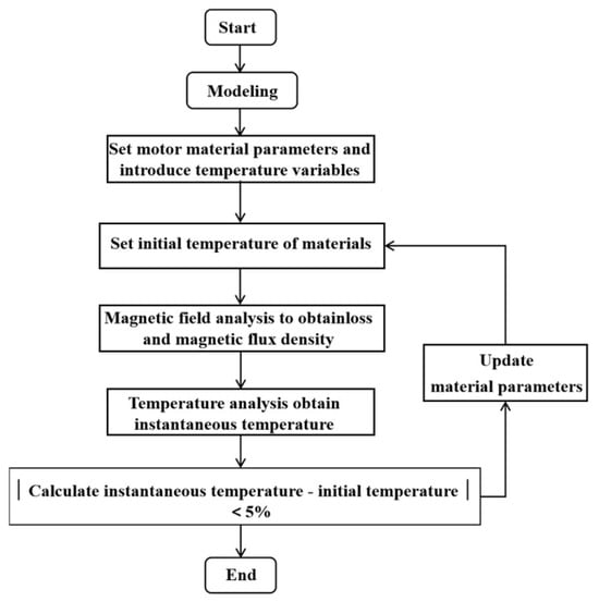
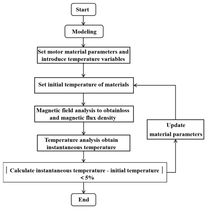
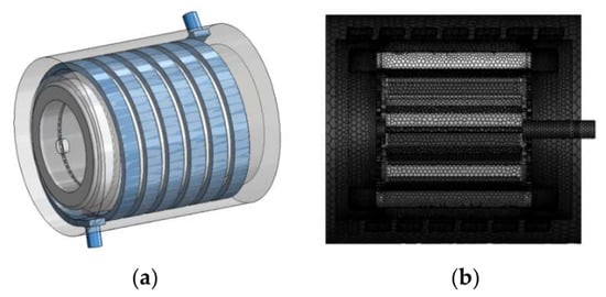
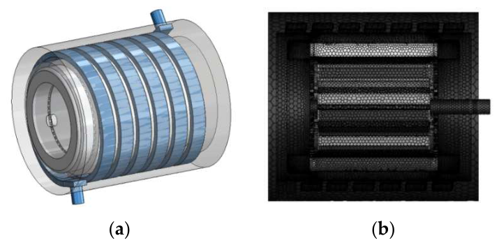
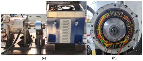
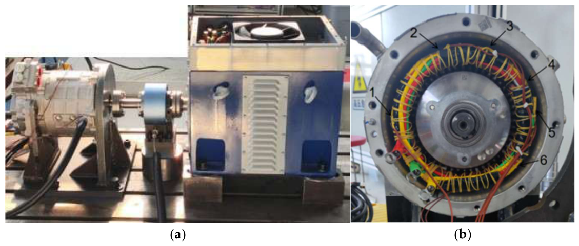
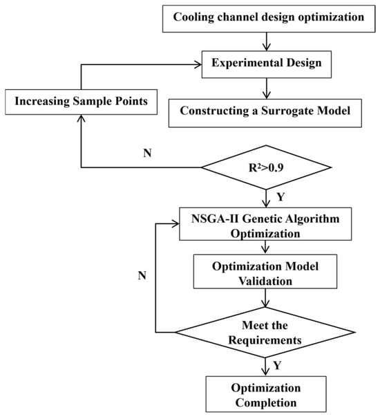
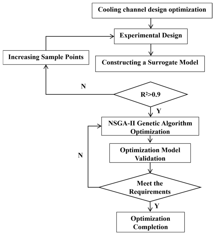
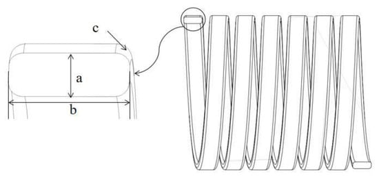
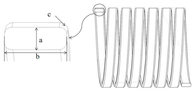
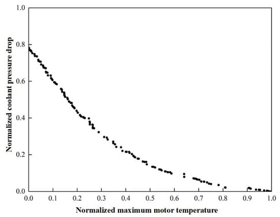
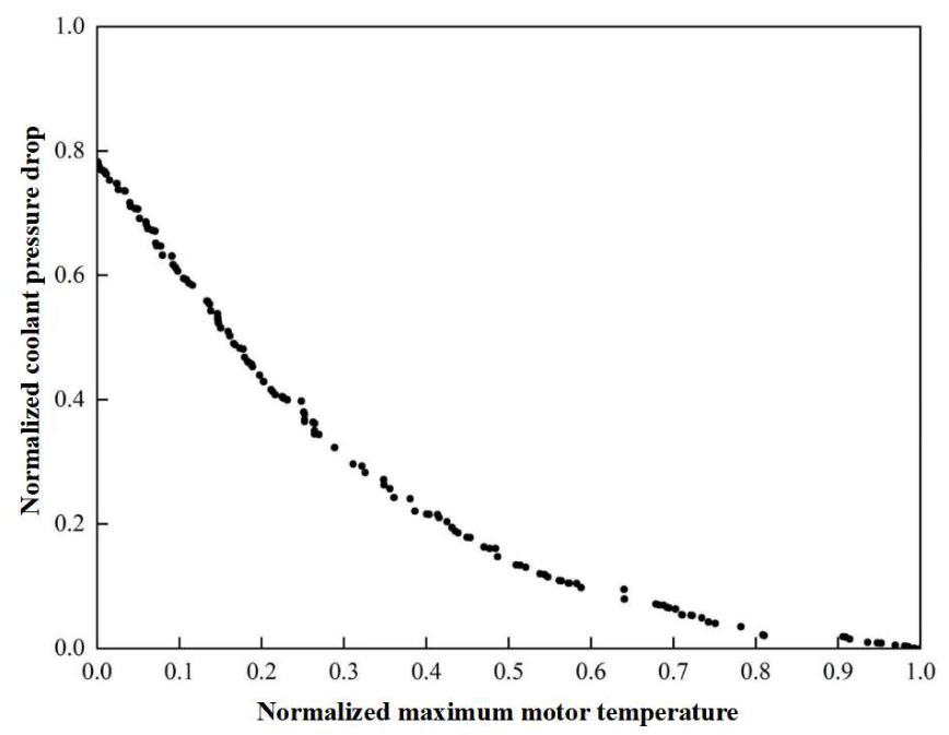
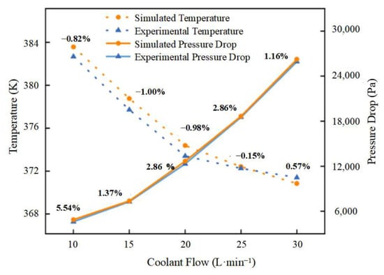
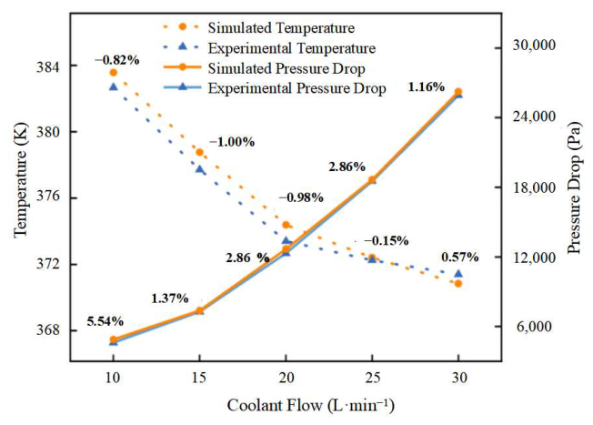
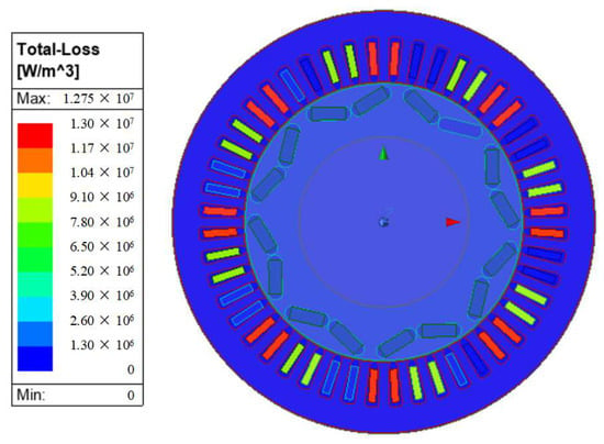
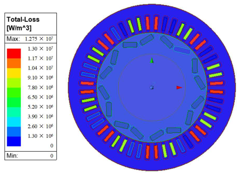
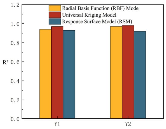
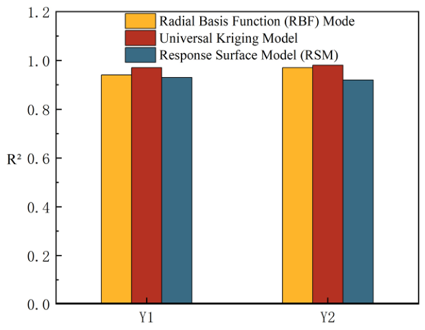
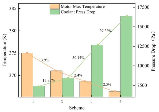
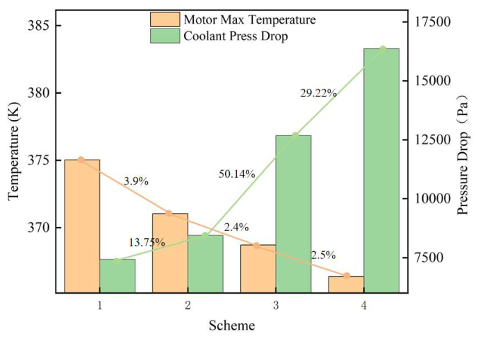
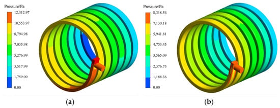
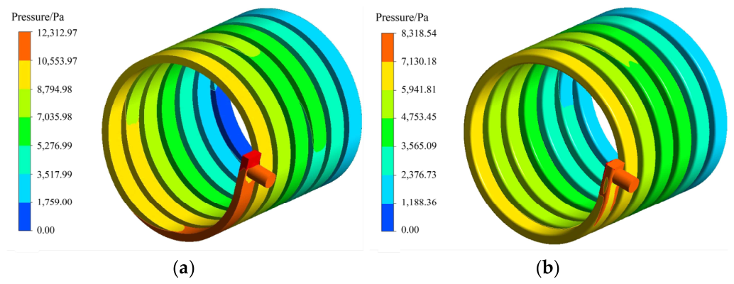
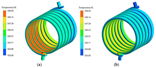
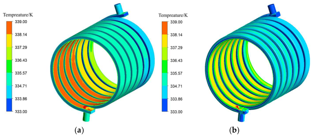
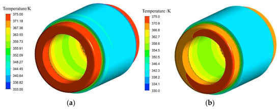
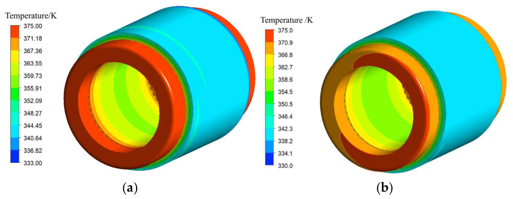

Disclaimer/Publisher’s Note: The statements, opinions and data contained in all publications are solely those of the individual author(s) and contributor(s) and not of MDPI and/or the editor(s). MDPI and/or the editor(s) disclaim responsibility for any injury to people or property resulting from any ideas, methods, instructions or products referred to in the content. |
© 2026 by the authors. Published by MDPI on behalf of the World Electric Vehicle Association. Licensee MDPI, Basel, Switzerland. This article is an open access article distributed under the terms and conditions of the Creative Commons Attribution (CC BY) license.