Tightly Coupled SLAM Algorithm Based on Similarity Detection Using LiDAR-IMU Sensor Fusion for Autonomous Navigation

Abstract

In recent years, the rise of unmanned technology has made Simultaneous Localization and Mapping (SLAM) algorithms a focal point of research in the field of robotics. SLAM algorithms are primarily categorized into visual SLAM and laser SLAM, based on the type of external sensors employed. Laser SLAM algorithms have become essential in robotics and autonomous driving due to their insensitivity to lighting conditions, precise distance measurements, and ease of generating navigation maps. Throughout the development of SLAM technology, numerous effective algorithms have been introduced. However, existing algorithms still encounter challenges, such as localization errors and suboptimal utilization of sensor data. To address these issues, this paper proposes a tightly coupled SLAM algorithm based on similarity detection. The algorithm integrates Inertial Measurement Unit (IMU) and LiDAR odometry modules, employs a tightly coupled processing approach for sensor data, and utilizes curvature feature optimization extraction methods to enhance the accuracy and robustness of inter-frame matching. Additionally, the algorithm incorporates a local keyframe sliding window method and introduces a similarity detection mechanism, which reduces the real-time computational load and improves efficiency. Experimental results demonstrate that the algorithm achieves superior performance, with reduced positioning errors and enhanced global consistency, in tests conducted on the KITTI dataset. The accuracy of the real trajectory data compared to the ground truth is evaluated using metrics such as ATE (absolute trajectory error) and RMSE (root mean square error).

1. Introduction

With the rapid advancement of science and technology, driverless technology has transitioned from a science fiction concept to a practical application. During this evolution, Synchronous Localization and Map Construction (SLAM) algorithms have emerged as a focal point of research in the field of robotics, as they facilitate localization without dependence on external satellite navigation. SLAM technology is not only essential for autonomous vehicles but also serves as the foundation for autonomous robot navigation and environmental sensing. Since Smith and Cheeseman first introduced the concept of SLAM in 1986 [1], research in this area has deepened significantly, continually propelling the progress of robotics.

In recent years, the performance of LiDAR and visual sensors has significantly improved, leading to widespread attention on SLAM algorithms that utilize these two types of sensors. While visual SLAM methods can efficiently extract feature points, they are vulnerable to varying lighting conditions and often lack robustness [2]. In contrast, LiDAR plays a crucial role in the field of autonomous driving due to its advantages, including insensitivity to lighting, precise distance measurement, and the ease of generating navigation maps [3].

However, even LiDAR-based SLAM algorithms encounter numerous challenges. The accuracy and stability of these algorithms are frequently tested in diverse environments. For example, in feature-degraded or expansive outdoor settings, existing SLAM algorithms often grapple with the problem of accumulated positioning errors. Consequently, developing a SLAM algorithm that can operate reliably across various environments and effectively mitigate accumulated errors has become a central focus of current research.

To address these challenges, this paper presents a tightly coupled SLAM (Simultaneous Localization and Mapping) algorithm framework based on factor graph optimization. The key innovations include the following points:

• In the point cloud feature extraction process, the constraint factor is established based on the depth distance between the target point cloud and the LiDAR sensor to calculate the adaptive curvature.
• During the factor graph optimization, a similarity test mechanism is established to enhance the selection of keyframes, ensuring that the process is more accurate and improving the overall accuracy of the algorithm.
• In the loop detection process, the traditional method of judgment based on Euclidean distance has been modified. The z-axis data, which tends to accumulate significant errors, is constrained, and similarity detection is performed on the two matching point cloud datasets to ensure the accuracy of the loop detection process.

The algorithm is designed to enhance the accuracy and reliability of SLAM (Simultaneous Localization and Mapping) systems by utilizing advanced techniques such as adaptive feature extraction, tightly coupled data integration, and similarity verification mechanisms. It addresses the significant localization inaccuracies and the imprecision in map creation that are often encountered in traditional laser SLAM methods. In doing so, it paves the way for substantial advancements in the development of autonomous vehicle technology.

2. Related Work

Since the introduction of the SLAM (Simultaneous Localization and Mapping) concept, researchers have developed numerous advanced algorithms tailored for various application scenarios and sensor types. Fast-SLAM, a SLAM algorithm based on particle filters, was proposed by Thrun S. et al. in 2002. Fast-SLAM introduced the RBPF (Rao-Blackwellised Particle Filter) algorithm, which decomposes the SLAM problem into two mutually independent sub-problems: robot pose estimation and posterior probability distribution of map coordinates [4]. Specifically, robot pose estimation is performed using a particle filter, while the posterior probability distribution of map coordinates is estimated through an extended Kalman filter. Fast-SLAM effectively handles nonlinear systems due to its particle filtering technique. However, in large environments or when odometry errors are significant, Fast-SLAM may require an increased number of particles to achieve improved estimation, which can lead to excessive computational costs. In the field of LiDAR-based SLAM, the Cartographer algorithm, a representative of graph-based optimization, introduces the concept of submaps. It combines CSM (Ceres Solver) with gradient optimization to match frames with submaps, improving matching accuracy and efficiency [5]. At the backend, the algorithm incorporates graph optimization, adding the current LiDAR frame and all previously established submaps to the loop closure detection module. It employs the branch and bound method to enhance search speed [6]. Cartographer demonstrates excellent performance in indoor environments with rich structural features. However, in feature-degraded environments or large outdoor environments, the positioning accuracy of this algorithm can be significantly affected [7].

With the widespread adoption of 3D LiDARs, 3D LiDAR-based SLAM algorithms have gradually become a research focus. Among them, the LOAM [8] algorithm proposed by Zhang et al. in 2014 utilizes curvature features for front-end registration and adopts partial ideas from iterative ICP [9] and its variants (such as PP-ICP [10], NICP [11], IMLS-ICP [12], GICP [13], and VGICP [14]) during the matching process. The algorithm assumes uniform motion for the LiDAR and employs linear interpolation for motion compensation, achieving remarkable results in practical applications. However, LOAM encounters the challenge of accumulated errors that cannot be effectively mitigated in large environments over extended periods of operation. To address this issue, the LEGO-LOAM [15] algorithm introduces IMU data fusion and loop closure detection mechanisms, significantly reducing these accumulated errors. Nevertheless, it has its limitations. In comparison to LOAM, LEGO-LOAM’s feature extraction strategy involves projecting the 3D point cloud onto a 2D image to distinguish ground points from non-ground points and eliminate noise. This method makes the algorithm highly sensitive to the conditions of the ground environment. The algorithm employs a loosely coupled approach to fuse IMU data with LiDAR point cloud data. Unlike purely LiDAR-based solutions, the integration of LiDAR with IMU takes advantage of the high-frequency motion information provided by the IMU to correct motion distortions in the point cloud. This yields a reliable initial value that helps the algorithm avoid local minima, enhances accuracy, and reduces computational complexity. However, the loosely coupled fusion approach used by this algorithm does not fully capitalize on the available sensor data.

In comparison to loose coupling, tight coupling demonstrates superior robustness and accuracy. This approach integrates LiDAR data and Inertial Measurement Unit (IMU) data to collaboratively construct a parameter vector, which is subsequently optimized and estimated. Currently, tight coupling represents a prominent area of research within the field of multisensor fusion. In this context, Ye et al. introduced the first open-source solution for tightly coupled three-dimensional LiDAR and IMU integration, known as LIO-Mapping [16]. The tightly coupled odometry algorithm in LIO-Mapping leverages the IMU more effectively than the Inertial-LOAM method, which only conducts data fusion prior to odometry. Furthermore, the mapping algorithm employed in LIO-Mapping incorporates a rotation constraint refinement technique to align the gravitational direction with the z-axis coordinate. Although LIO-Mapping surpasses SLAM solutions that depend exclusively on LiDAR or those that utilize a loose coupling of IMU and LiDAR, it still necessitates stable initialization and pre-integration of the IMU.

In recent years, SLAM algorithms based on iterative extended Kalman filters have garnered significant attention. In 2021, the MaRs Lab at the University of Hong Kong proposed FAST-LIO [17], a SLAM algorithm optimized using iterative extended Kalman filtering. This algorithm adopts a tightly coupled approach to processing sensor data, enhancing the accuracy and robustness of optimization. However, due to its reliance on Kalman filtering, which only considers the mutual constraints between two frames, FAST-LIO lacks global consistency. FAST-LIO2 [18] builds upon the improvements of FAST-LIO. To enable the algorithm to naturally adapt to LiDAR with different scanning modes and achieve faster computation, FAST-LIO2 omits the time-consuming feature extraction module. Instead, it adopts a direct method to uniformly process all point cloud data and calculates point-to-plane residuals. It utilizes a novel data structure called ikd-Tree [19], a dynamic kd-Tree, to store point cloud data. Compared to existing dynamic data structures such as octree, R*-tree, and nanoflann k-d tree, ikd-Tree exhibits superior overall performance. However, in large-scale scenarios with vast amounts of point cloud data, the time required for ikd-Tree to maintain the dynamic balance of the tree structure becomes non-negligible. This limitation precludes FAST-LIO2 from achieving real-time mapping tasks in large-scale scenarios. Faster-LIO addresses this challenge by introducing an incremental sparse voxel (iVox) data structure in place of ikd-Tree, effectively reducing the time required for point cloud registration without significantly compromising the accuracy of the odometer. Faster-LIO [20] achieves a speed that is 1.5–2 times faster than FAST-LIO2. Nevertheless, the use of Kalman filtering for optimization, which only considers the mutual constraints between two frames, still poses a challenge in terms of global consistency for Faster-LIO. Point-LIO [21] is an innovative LiDAR inertial odometry method that offers extremely high odometry output frequency and is particularly suited for situations with severe vibrations and high-speed motion. However, Point-LIO has some drawbacks, such as the difficulty in establishing relationships between individual point clouds, which can affect the algorithm’s accuracy, and the inability to utilize semantic information of point clouds in real time. EfficientLIO-Net [22] is the first fully end-to-end efficient 3D LiDAR odometry framework, proposing a projection-based three-dimensional point cloud representation method and feature learning approach, outperforming all recent learning-based LiDAR odometry methods. However, this method consumes a significant amount of resources, making real-time operation challenging.

In conclusion, current SLAM algorithms exhibit distinct advantages and limitations across various dimensions. The tightly coupled SLAM framework, which is predicated on point cloud feature optimization and presented in this study, seeks to offer a more dependable and efficient solution for the practical implementation of autonomous driving technology by addressing the deficiencies of existing algorithms. This framework aims to enhance global consistency, improve robustness, and decrease computational complexity, thereby facilitating real-time and precise mapping and localization across diverse scenarios.

3. Materials and Methods

3.1. Algorithm Framework

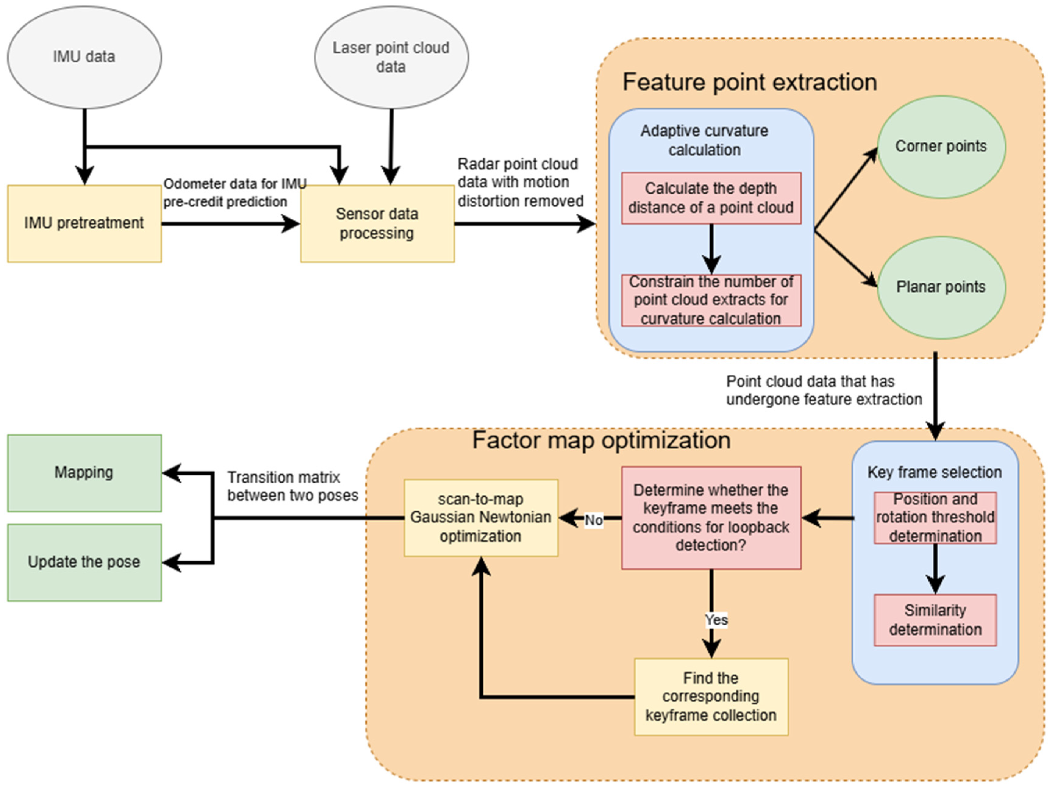
This paper presents a tightly coupled Simultaneous Localization and Mapping (SLAM) algorithm that utilizes factor graph optimization. To address the motion aberrations that occur during the acquisition of radar point clouds, this algorithm diverges from the uniform motion assumption and linear interpolation methods employed in the LOAM algorithm. Instead, it leverages high-frequency Inertial Measurement Unit (IMU) data to ascertain the real-time orientation of the radar during the acquisition of each frame, thereby compensating for the motion of the collected point cloud data and effectively mitigating motion aberrations. Unlike SLAM algorithms that rely on filtering techniques, the proposed algorithm treats all states as variables and formulates motion and observation equations as constraints among these variables. It constructs an error function, which is subsequently minimized to derive the optimal orientation. The framework of the proposed algorithm is illustrated in Figure 1, which is organized into three primary components:

• IMU Odometry Module: The data from the Inertial Measurement Unit (IMU) are pre-integrated by incorporating the position estimation data derived from LiDAR odometry. This integration serves to furnish high-precision initial value information for the LiDAR odometry process. Furthermore, the IMU factor is incorporated into the subsequent factor graph optimization solution. Additionally, the IMU bias is included as a factor in the optimization process, necessitating its repropagation following any updates.
• LiDAR Odometry Module: The a priori information of IMU odometry is used to compensate for the motion distortion of the point cloud data and is used as the initial value for optimization. After that, the feature point cloud is extracted according to the curvature magnitude, and when the robot’s position change exceeds the threshold value, the position state at this moment is set as a keyframe and added to the keyframe queue. For the corner points and plane points, the distance from the point to the straight line and the point to the plane is used as the loss function, and the optimized position is obtained iteratively by using the nonlinear optimization method.
• Loopback Detection Module: LiDAR odometry is employed to establish the key frame queue through a methodology that utilizes two-dimensional plane distance to identify the keyframe and its adjacent keyframes for distance calculation. When the computed distance falls below a predetermined threshold, it is interpreted as a loop closure. Subsequently, the identified keyframes are incorporated into the factor graph, and the associated pose transformation is determined using the Gauss–Newton method, thereby finalizing the loop closure detection process.

Figure 1. Algorithm flowchart based on feature optimization.

Figure 1. Algorithm flowchart based on feature optimization.

3.2. IMU Odometer Module

The algorithm presented in this paper is a SLAM framework of IMU odometry and LiDAR odometry tightly coupled. In the IMU pre-integration sessions, the main task is to utilize the IMU data to provide a better initial estimate of the vehicle position. Because most of the current LiDAR has a frequency of 10 Hz, the robot will be displaced and rotated during the acquisition of a frame of point cloud, which leads to a decrease in the accuracy of point cloud matching. While the IMU generally has a frequency of more than 200 Hz, it can provide a better initial position for the matching between two frames of the point cloud. In the IMU pre-integration sessions, we define the measured values of acceleration and angular velocity of the IMU by Equations (1) and (2):

$${\stackrel{⏜}{w}}_t=w_t+b_t^w+n_t^w$$

(1)

$${\stackrel{⏜}{a}}_t=R_t^{BW}(a_t-g)+b_t^a+n_t^a$$

(2)

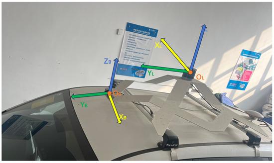
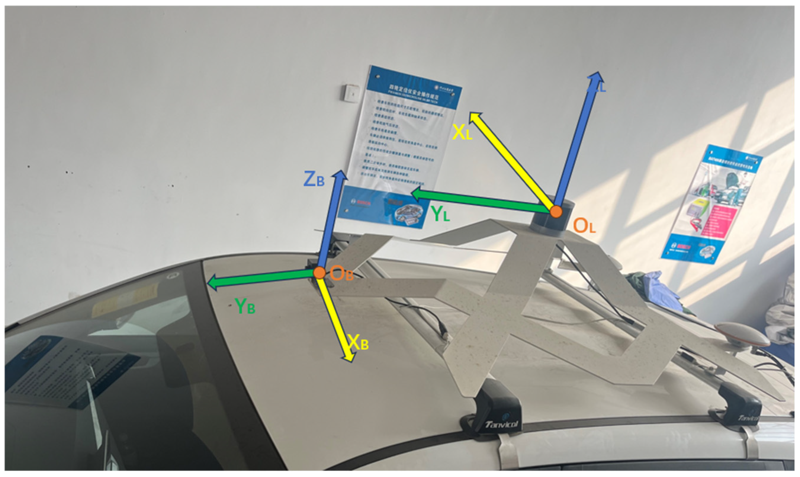
where ${\stackrel{⏜}{w}}_t$ and ${\stackrel{⏜}{a}}_t$ are the observed values of angular velocity and acceleration, $b_t^w$ and $b_t^a$ are the bias of angular velocity and acceleration, $n_t^w$ and $n_t^a$ are the angular velocity noise and acceleration noise, $R_t^{BW}$ denotes the rotation matrix from the world coordinate system to the robot coordinate system, and $g$ is the gravity vector in the world coordinate system [23]. The schematic diagram of the vehicle coordinate system and the LiDAR coordinate system is shown in Figure 2.

Figure 2. Schematic diagram of the vehicle coordinate system (O_BX_BY_BZ_B) and the LiDAR coordinate system (O_LX_LY_LZ_L).

By measuring the values of angular velocity and acceleration, the equations of motion can be used to calculate the robot’s velocity, position, and rotation at the moment $t+\Delta t$:

$$v_{t+\Delta t}=v_t+g\Delta t+R_t({\stackrel{⏜}{a}}_t-b_t^a-n_t^a)\Delta t$$

(3)

$$p_{t+\Delta t}=p_t+v_t\Delta t+{\displaystyle \frac{1}{2}}g\Delta t^2+{\displaystyle \frac{1}{2}}{R}_t({\stackrel{⏜}{a}}_t-b_t^a-n_t^a)\Delta t^2$$

(4)

$$R_{t+\Delta t}=R_t\exp (({\stackrel{⏜}{w}}_t-b_t^w-n_t^w)\Delta t)$$

(5)

However, it is difficult to maintain high accuracy over a long period of time, no matter how high the accuracy of the IMU is, and the integration will integrate the error as well, resulting in the IMU odometer only being used for position correction over a short period of time. Therefore, it is necessary to fuse the odometer information obtained from the laser odometer for pre-integration to achieve the correction.

3.3. LiDAR Odometer Module

The LiDAR odometry module primarily focuses on the extraction of corner points and planar features from point cloud data, the identification of keyframes, and the optimization of these keyframes through the sliding window approach to develop a factor map. During the optimization phase, residual equations are formulated based on point-to-line and point-to-plane distances. The positional transformation between two frames of the point cloud is determined by iteratively applying the Gauss–Newton method.

3.3.1. Adaptive Curvature Feature Extraction

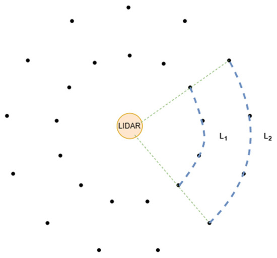
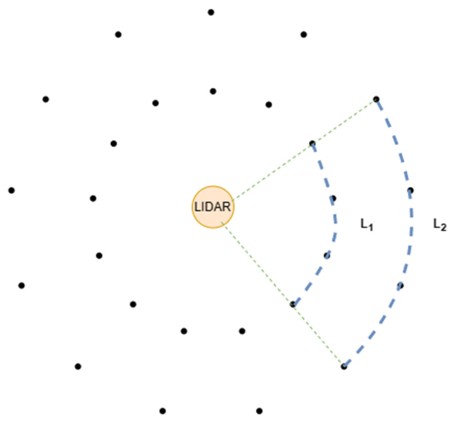
Traditional feature extraction methods such as LOAM use a method that derives the curvature by calculating the vector sum of the key point $i$ and the five points before and after it and then distinguishes between corner and plane points by the curvature magnitude [24]. However, this method does not take into account the denseness of the point cloud, and most of the LiDARs on the market today operate with rotational scanning, with a horizontal scanning resolution of 0.2° for a 16-line LiDAR, for example. Therefore, it will make the point cloud of the same line beam produce the phenomenon of dense in the near distance and sparse in the far distance; this is shown in Figure 3.

Figure 3. This figure is a schematic diagram of the LiDAR point cloud extraction process.

If we still follow the traditional feature extraction method and just calculate the curvature of the key point $i$ and the five points before and after it, the line segments composed of these point clouds at a close distance will be too short, and the line segments composed of these point clouds at a farther distance will be too long. The curvature derived in both cases does not accurately describe the smoothness at that location, which can degrade the accuracy of the feature extraction process. To address this problem, the paper proposes a base and distance adaptive curvature feature extraction method. First, the depth distance $h$ between each point and the LiDAR is calculated according to the time of flight method. Then, a constraint factor $a$ is established based on the distance between the key point $i$ and the radar. The number of point clouds computed for different distances is controlled by the constraint factor. When calculating curvature, for key points with close distances, the number of neighboring points selected will be increased to ensure the integrity of the curve. For key points with far distances, the number of neighboring points selected will be decreased to ensure that the curve is not too long and can more accurately reflect the curvature of the point.

For the curvature calculation of key point $i$, the following formula is used in this paper:

$$c={\displaystyle \frac{1}{|S|\cdot \parallel X_{(k,i)}^L\parallel }}\parallel \sum _{j\in S,j\ne i}(X_{(k,i)}^L-X_{(k,j)}^L)\parallel$$

(6)

When calculating the curvature of the point cloud $i$, select the relationship between the number of adjacent point clouds $S$ and the depth distance $h$ as follows:

$$S\in \left[(10,h\le 10),(8,10<h\le 20),(6,20<h\le 30),(4,h>30)\right]$$

After the curvature calculation for each point is completed, in order to prevent two points on different planes from being mistaken as two neighboring points on the same plane during the LiDAR scanning process. In this paper, by comparing the depth between two neighboring points, the two points whose depth difference exceeds the threshold value are judged to be in different planes and are eliminated in the subsequent feature extraction process.

3.3.2. Factor Graph Optimization

This paper presents the development of a local map comprising multiple point cloud keyframes, which is optimized through the local map sliding method for keyframes. The traditional LOAM algorithm operates by transforming corner and plane points from the current frame into the laser point cloud of the preceding frame using initial data. Subsequently, it identifies corresponding line and plane features for matching, ultimately determining the positional changes between the two frames. However, a notable limitation of this methodology is that the features present in a single frame may not be sufficiently abundant, potentially resulting in inaccuracies in feature matching and a consequent reduction in overall precision. To address this issue, certain algorithms have begun to utilize a local map that incorporates all keyframes preceding the current frame to enhance the accuracy of feature matching. Nonetheless, as the number of keyframes included in the local map increases, the efficiency of the matching process tends to decline.

To enhance efficiency, this study employs a local map sliding technique for keyframes to construct local maps of historical keyframes. Initially, the point cloud data captured at a specific moment, provided certain conditions are satisfied, is designated as a keyframe. Subsequently, these keyframes are incorporated into a keyframe collection, with the thresholds for positional and rotational changes established at 1 m and 10 degrees, respectively.

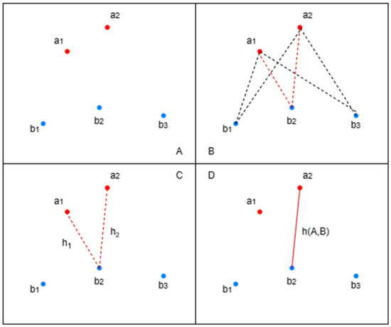
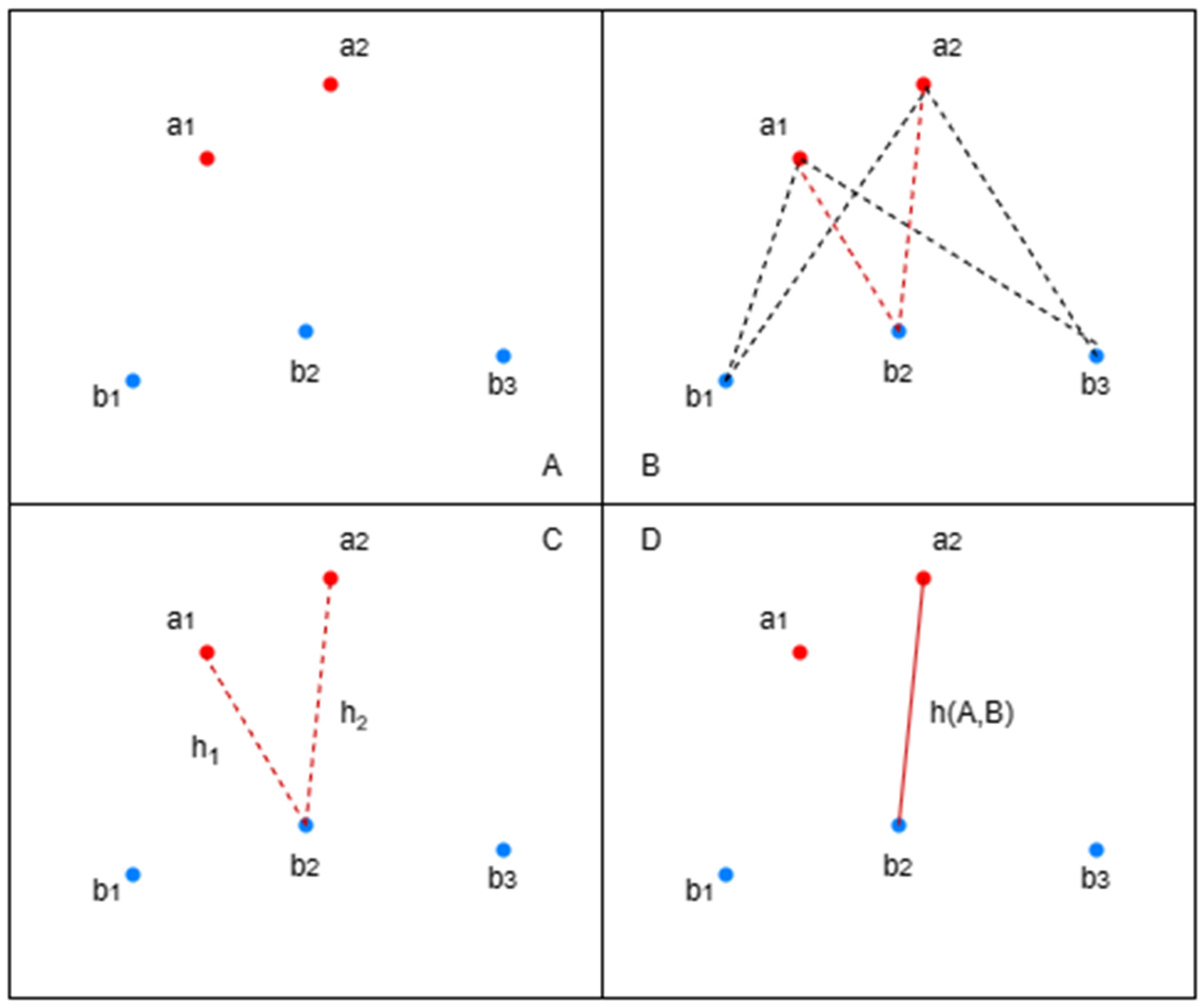
To refine the selection process for keyframes, this paper introduces a similarity detection mechanism. Upon identifying a keyframe that meets the specified positional and rotational change thresholds, the similarity between this keyframe and the preceding one is assessed. This mechanism primarily utilizes the Hausdorff distance, which quantifies the maximum discrepancy between two sets, as illustrated in Figure 4.

Figure 4. This is the schematic diagram of Hausdorff distance.

Suppose there are two sets $A=\{a_1,\dots ,a_p\}$ and $B=\{b_1,\dots ,b_p\}$, then the Hausdorff distance between the two sets is defined as follows:

$$H(A,B)=\max (h(A,B),h(B,A))$$

(7)

Among them, $H(A,B)$ is called the bidirectional Hausdorff distance between sets $A$ and $B$, which is the most basic form of Hausdorff distance; $h(A,B)$ and $h(B,A)$ are the unidirectional Hausdorff distances from set $A$ to set $B$ and from set $B$ to set $A$, respectively, which are calculated as follows:

$$\left\{\begin{array}{c}h(A,B)={\max }_{a\in A},{\min }_{b\in B}\parallel a-b \parallel \\ h(B,A)={\max }_{b\in B},{\min }_{a\in A}\parallel a-b \parallel \end{array}\right.$$

(8)

In fact, $h(A,B)$ first calculates the distance $\parallel a_i-b_j\parallel$ between each point $a_i$ in the set $A$ and the midpoint $b_j$ in the set $B$ closest to the point $a_i$ (if there are 100 points in the set $A$, there are 100 minimum values above) and then sorts and then takes the maximum value in the distance (the maximum value of 100 minimum values) as the value of $h(A,B)$, and $h(B,A)$ can be obtained in the same way. The value $H(A,B)$ obtained by calculating the Hausdorff distance can judge the similarity relationship between two adjacent keyframes, avoid the high similarity between consecutive keyframes, and make the subsequent optimization process more efficient and accurate.

In the interim, this study establishes a threshold for the number of keyframes. When the quantity of keyframes remains below this threshold, the local map is constructed using all available keyframes. Conversely, if the number of keyframes surpasses the threshold, the oldest keyframes are eliminated from the ensemble, and the local map is subsequently formed by incorporating the new keyframes. This approach guarantees the integrity of valid features while also considering the efficiency of the matching process. The pseudo-code for this methodology is presented below (Algorithm 1):

Algorithm 1: Sliding window method with similarity detection.

1   Input: laser point cloud frame sequence Si, i = 1, 2, … 2   Output: bitwise transformation between two frames T 3   begin 4   for i = 1, 2, … do 5   if i == 1 then 6       Pre-mark Si as a key 7          calculate $H(S_{\mathrm{i}},S_{\mathrm{i}-1})$ 8          if $H(S_{\mathrm{i}},S_{\mathrm{i}-1})$ > $h_1$ 9          Mark Si as a keyframe 10        end if 11   end if 12   $F_{\mathrm{i}}\leftarrow S_{\mathrm{i}}$ 13   Splice local map Mi 14  $\begin{array}{c}{M}_{\mathrm{i}}\end{array}=F_{\mathrm{i}}\cup F_{\mathrm{i}-1}\cup \cdots \cup F_{\mathrm{i}-n}$ 15   if i > 25 16   Removal $F_{\mathrm{i}-25}$ 17   $\begin{array}{c}{M}_{\mathrm{i}+1}\end{array}=F_{\mathrm{i}+1}\cup F_{\mathrm{i}}\cup \cdots \cup F_{\mathrm{i}-24}$ 18   end if 19   The Gaussian Newton method is used to solve the position transformation       between two frames of the point cloud 20   return T 21   end for 22   end

The specific steps for factor graph optimization involve calculating the residual distance between the extracted features and the corresponding edges or planes, which is obtained from the following formula:

$$d_{e_k}={\displaystyle \frac{\left|(p_{i+1,k}^e-p_{i,u}^e)\times (p_{i+1,k}^e-p_{i,v}^e)\right|}{\left|p_{i,u}^e-p_{i,v}^e\right|}}$$

(9)

$$d_{p_k}={\displaystyle \frac{\left|\begin{array}{c}(p_{i+1,k}^p-p_{i,u}^p)\\ (p_{i,u}^p-p_{i,v}^p)\times (p_{i,u}^p-p_{i,w}^p)\end{array}\right|}{\left|\begin{array}{c}(p_{i,u}^p-p_{i,v}^p)\times (p_{i,u}^p-p_{i,w}^p)\end{array}\right|}}$$

(10)

where $k$, $u$, $v$, and $w$ are feature indices of different points in the map set. $p_{i, u}^e$ and $p_{i,v}^e$ form edge features, while $p_{i,u}^p$, $p_{i,v}^p$, and $p_{i,w}^p$ form plane features. The Gauss–Newton method is then used to solve for the optimal transformation by minimizing as follows:

$$\underset{T_{i+1}}{\min }\left\{\sum _{p_{i+1, k}^e\in F_{i+1}^e}{d}_{e_k}+\sum _{p_{i+1, k}^p\in F_{i+1}^p}{d}_{p_k}\right\}$$

(11)

Finally, we can obtain the relative transformation $\Delta T_{i,i+1}$ between ${\mathrm{x}}_i$ and ${\mathrm{x}}_{i+1}$, which is the LiDAR odometry factor linking these two poses:

$$\Delta T_{i, i+1}=T_i^{\mathsf{{\rm T}}}{T}_{i+1}$$

(12)

3.4. Loopback Detection Module

Since some errors are unavoidable during the operation of the robot, loopback detection is needed to eliminate the accumulated errors. Nowadays, most of the loopback detection algorithms are based on the Euclidean distance between the current position and the historical position to determine whether to perform loopback detection or not [25], i.e.:

$$d_{ab}=\sqrt{\sum _{i=1}^n{\left(x_i-y_i\right)}^2}$$

(13)

The measurement methodology employed in this study, which integrates laser radar with an inertial unit, often results in considerable deviation along the Z-axis following extended operational periods. Consequently, this research limits the dimensional variables in the aforementioned formula to two, focusing on the two-dimensional distance within the plane that separates the current position from the historical position.

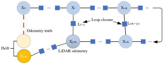
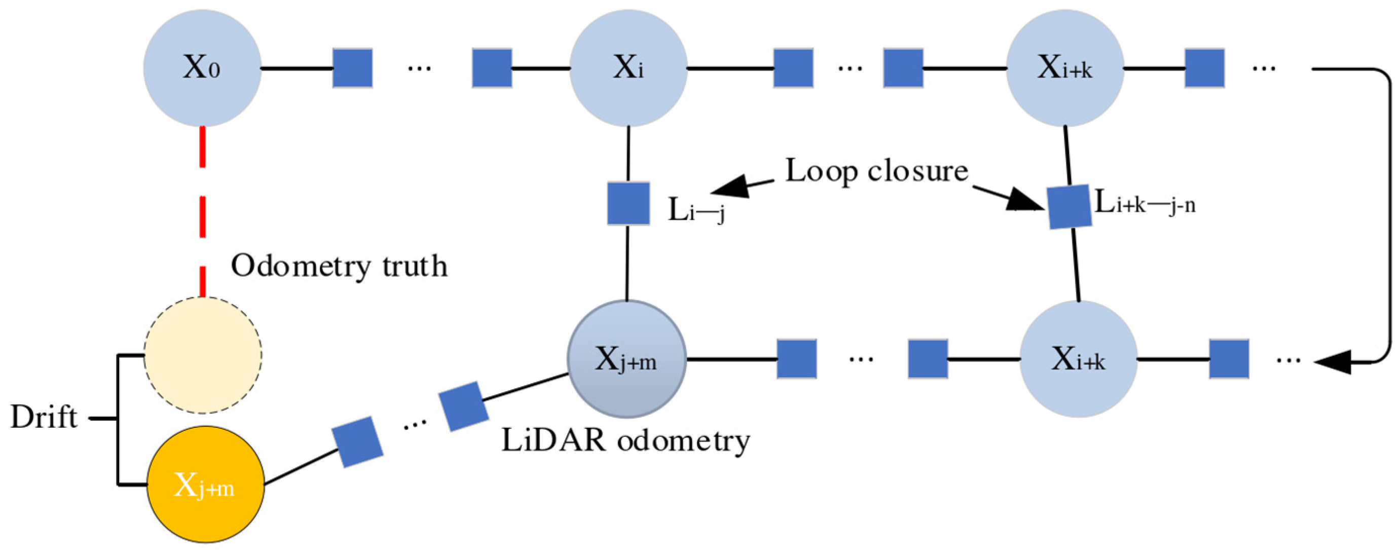
When this distance falls below a predetermined threshold, relevant keyframes within this proximity are identified from the historical keyframes based on the current key frame positions, thereby facilitating the construction of a local map utilizing these keyframes. It is important to note that the cumulative errors associated with the LiDAR odometer may result in drift, which can erroneously enable loopback detection between two incorrect key frame datasets, as illustrated in Figure 5.

Figure 5. This is the schematic diagram of cumulative error in loop detection.

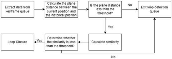
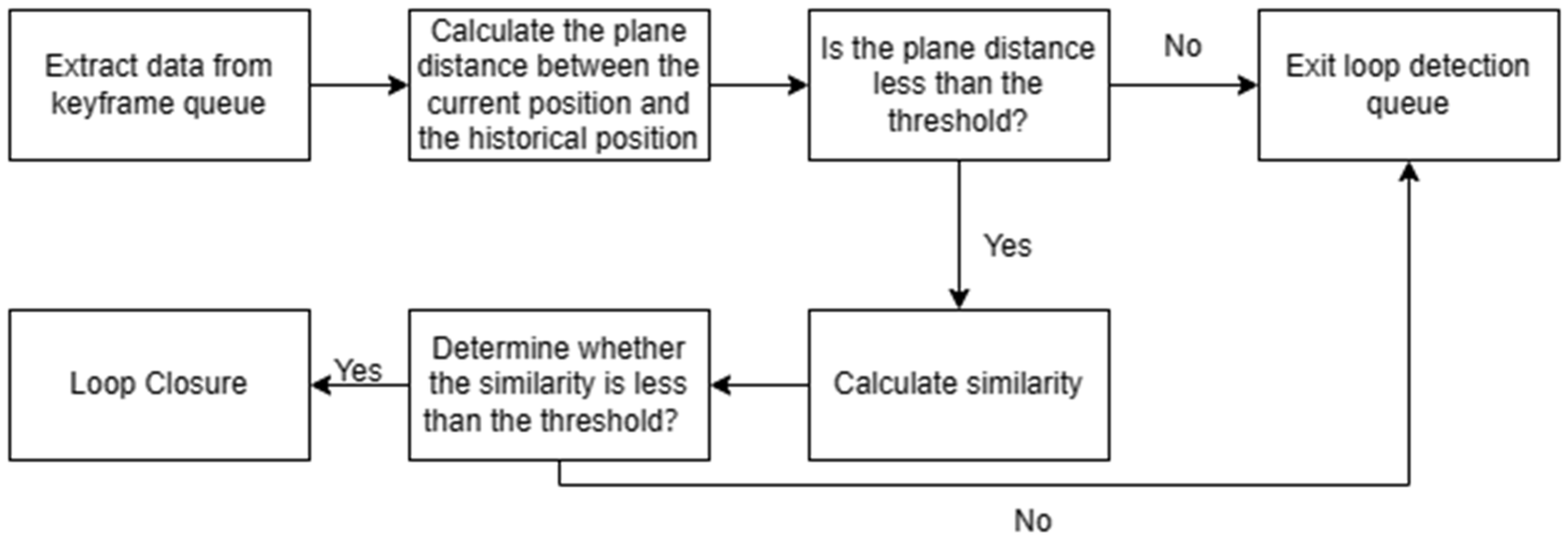
To enhance the recall rate of loopback detection, this study incorporates a similar discrimination mechanism alongside the assessment of loopback detection based on the spatial distance between the current position and historical positions. The details of this mechanism have been previously outlined and will not be reiterated here. By evaluating the similarity between the current keyframe data and historical keyframe data, it is possible to ascertain whether the conditions for loopback detection are satisfied. The loop detection methodology proposed in this research is illustrated in Figure 6.

Figure 6. This is the loop detection and determination flow chart.

For the keyframe data that meet the loopback condition, it will be matched and optimized with the corresponding local map, and finally, the optimal pose that eliminates the cumulative error is obtained.

4. Experimental Results and Analysis

The algorithm delineated in this study is engineered to accommodate a variety of driving conditions, encompassing differing weather scenarios and vehicle velocities. It demonstrates proficiency in localization and map construction in environments characterized by low illumination and the absence of GPS signals. Additionally, the algorithm has been effectively implemented in high-speed highway contexts, showcasing its robustness and precision across varying speed parameters, thereby affirming its versatility across a spectrum of velocities. This research employs the KITTI dataset alongside external real-world scenarios to evaluate the algorithm’s performance. The experimental environment is configured using the Robot Operating System (ROS) [26] on Ubuntu 20.04, with the hardware specifications detailed in Table 1.

Table 1. Experimental hardware configuration table.

	Configuration
Processor	Intel (R) Core (TM)i9-12900H 2.50 GHz
Graphics card	NVIDA GeForce RTX3060 laptop GPU
Memory	16G
Hard disk	1T

In this paper, trajectory accuracy is utilized as an evaluation index to evaluate the trajectory data through EVO, and the trajectory accuracy is measured by the KITTI official website method.

4.1. Test Experiments on the KITTI Dataset

This manuscript presents a detailed account of our experimental methodology for assessing odometrics and poses deviations utilizing sequences 07 and 09 from the KITTI dataset. The initial phase involved the acquisition of sensor data for these sequences, which were then systematically organized into comprehensive data packages. Following this, we performed a comparative analysis of our proposed algorithm against several state-of-the-art open-source algorithms, specifically ALOAM, an enhancement of the LOAM framework; the lightweight LEGO-LOAM introduced in 2018; and the tightly coupled sensor-based LIO-SAM. Each algorithm underwent rigorous testing on the KITTI dataset to generate map trajectory data. Ultimately, we employed the EVO (1.16) assessment software to conduct a meticulous analysis of the trajectory data, thereby quantifying the deviations observed. This systematic approach facilitates a thorough and transparent evaluation of our algorithm’s performance in relation to existing benchmarks.

4.1.1. Odometer Deviation Experiments

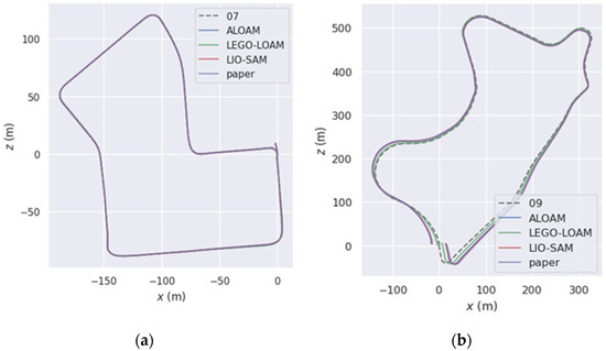
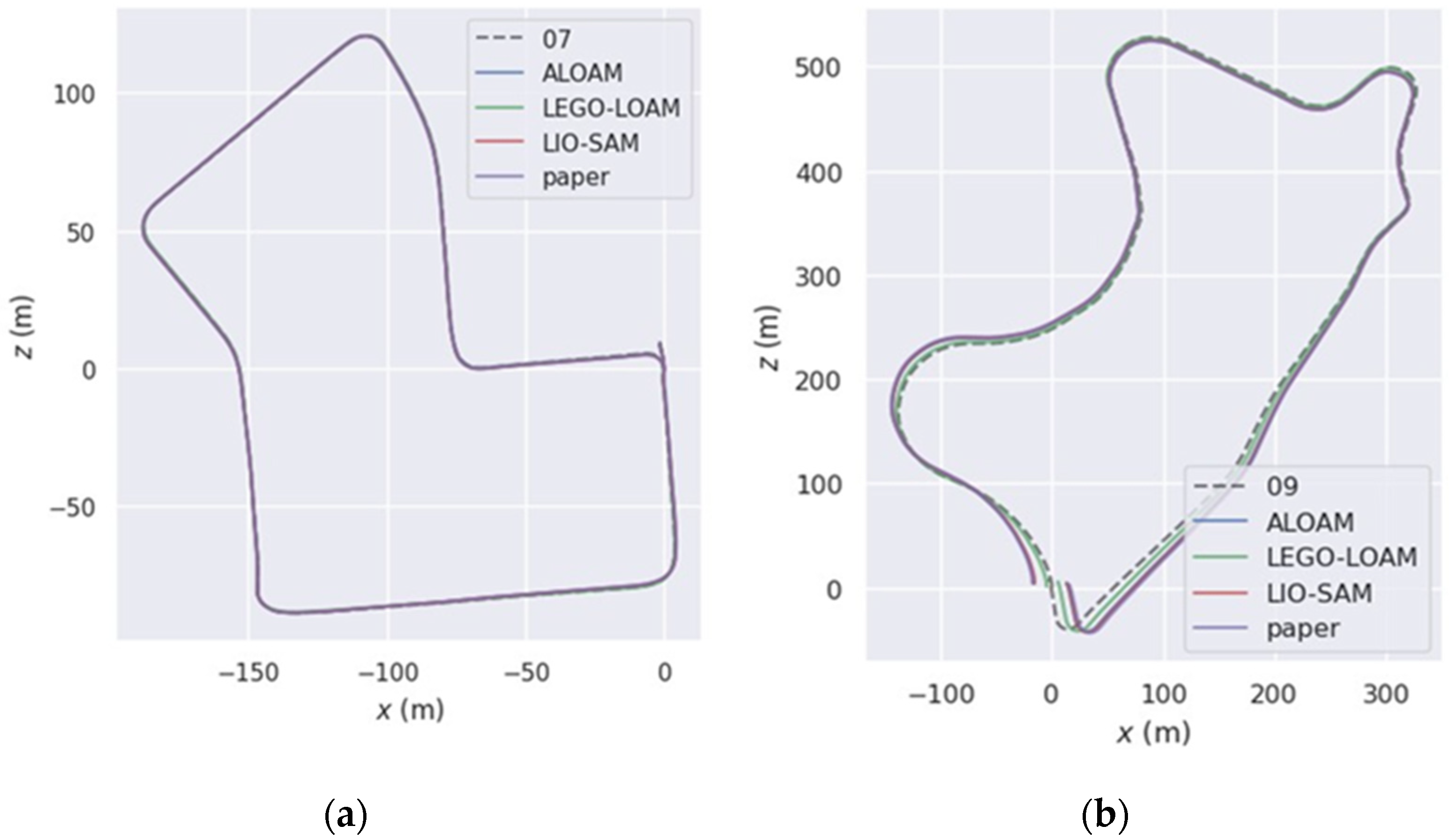
In the odometer bias experiment, this paper uses different algorithms to get the corresponding trajectory information by predicting the KITTI dataset 07 and 09 sequences and then compares it with the real trajectory downloaded from the KITTI official website to get the trajectory accuracy of different algorithms. As shown in Figure 7 for the trajectory comparison graph of EVO evaluation, it can be seen that the algorithms in this paper have better performance in both datasets and are closer to the real trajectory in most moments.

Figure 7. (a) The trajectories of the algorithm in this article are compared with other algorithms on the KITTI dataset 07 sequence and (b) the trajectories of this algorithm are compared with other algorithms on the KITTI dataset 09 sequence.

To facilitate a more intuitive comparison of the trajectory accuracies among various algorithms, the absolute trajectory errors assessed by EVO for the 07 sequence are presented in Table 2. The data indicate that the algorithm proposed in this study demonstrates superior performance across three key metrics: mean error (Mean), minimum error (Min), and root mean square error (RMSE). When compared to the three open-source algorithms—ALOAM, LEGO-LOAM, and LIO-SAM—the proposed algorithm exhibits improvements of 14.1%, 21.8%, and 6.2% in the mean error index, respectively. In terms of minimum error, the proposed algorithm achieves reductions of 0.06 m, 0.18 m, and 0.1 m. Furthermore, with respect to the root mean square error (RMSE) index, it realizes error reductions of 20.6%, 44.1%, and 26%.

Table 2. Absolute error data of odometry for each algorithm in the 07 sequence of the KITTI dataset.

Method	Absolute Trajectory Error (m)
	Mean	Min	RMSE
ALOAM	0.71	0.14	0.68
LEGO-LOAM	0.78	0.26	0.84
LIO-SAM	0.65	0.18	0.73
Ours	0.61	0.08	0.54

The real trajectory length of the KITTI dataset 09 sequence is larger, as shown in Table 3 for the relative trajectory error evaluated by EVO, which can reflect the trajectory accuracy of each algorithm in the unit length. From the data in the table, it can be seen that the algorithm proposed in this paper and the LIO-SAM are better in the average value of the error, and the accuracy of this paper’s algorithm is better than that of the ALOAM and LEGO-LOAM by 9.7% and 23.8%. While in the two indexes of error minimum and root mean square error, the algorithm of this paper and the ALOAM algorithm are more excellent.

Table 3. The relative error data of odometry for each algorithm in the KITTI dataset 09 sequence.

Method	Relative Trajectory Error (m)
	Mean	Min	RMSE
ALOAM	3.00	0.31	3.15
LEGO-LOAM	3.57	0.95	3.71
LIO-SAM	2.72	0.33	3.19
Ours	2.71	0.32	3.17

4.1.2. Position Deviation Experiment

In the positional deviation experiment, not only the deviation in distance between the trajectories produced by each algorithm and the real trajectory is considered, but also the rotational deviation of each position will be taken into account. Since the pose error in this experiment is a combined value of a distance error and an angular error, the units of this error are dimensionless. The bit pose accuracies evaluated by EVO in the KITTI dataset 07 and 09 sequences are shown in Table 4 and Table 5.

Table 4. Pose error data of various algorithms in the KITTI dataset 07 sequence.

Method	Absolute Trajectory Error (Dimless)
	Mean	Min	RMSE
ALOAM	2.51	2.45	2.51
LEGO-LOAM	2.48	2.07	2.50
LIO-SAM	2.47	1.74	2.51
Ours	2.45	1.72	2.49

Table 5. Pose error data of various algorithms in the KITTI dataset 09 sequence.

Method	Absolute Trajectory Error (Dimless)
	Mean	Min	RMSE
ALOAM	3.01	0.62	3.26
LEGO-LOAM	3.56	1.90	3.71
LIO-SAM	2.73	0.34	3.18
Ours	2.70	0.33	3.17

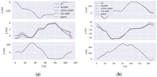
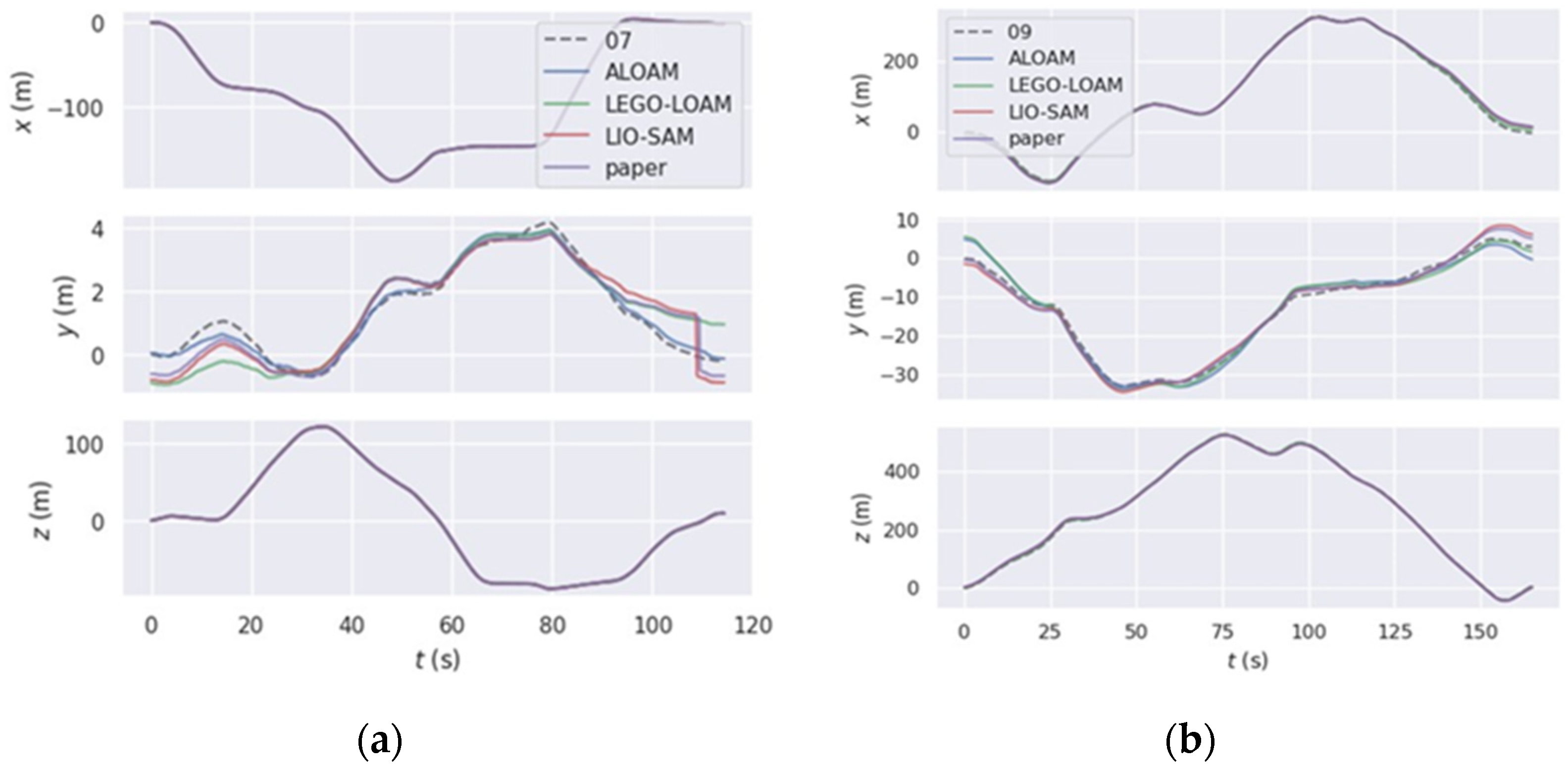
From the data in the table, it can be seen that the algorithm proposed in this paper still has a good performance in positional accuracy after adding the rotational error index. Taking the KITTI dataset 07 sequence as an example, in terms of the average error value, the accuracy is improved by 10.3%, 24.2%, and 1.1% compared with the other three algorithms; in terms of the minimum error, the accuracy is close to that of LIO-SAM and substantially higher than that of LEGO-LOAM; and in terms of the root mean square error index, the algorithm in this paper improves by 2.8% and 14.6% compared with ALOAM and LEGO-LOAM, respectively. The deviations in the four algorithms on the X, Y, and Z axes are shown in Figure 8, which shows that the proposed algorithm has the highest accuracy in most of the processes. From the above data, it can be concluded that the algorithm is more accurate for the positional localization of the robot. At the same time, according to the document “robust reconstruction of industrial scenes” [27], the trajectory accuracy can be used as an indirect indicator to measure the mapping accuracy, so the method proposed in this paper also has advantages in the construction of 3D maps.

Figure 8. (a) The deviation in the algorithm in this article is compared with other algorithms on the x, y, and z axes of the KITTI dataset 07 sequence and (b) the deviation in the algorithm in this article is compared with other algorithms on the x, y, and z axes of the KITTI dataset 09 sequence.

4.2. Real-Scene Test Experiment

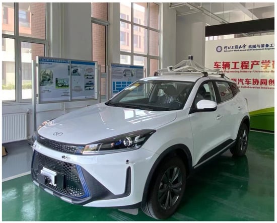
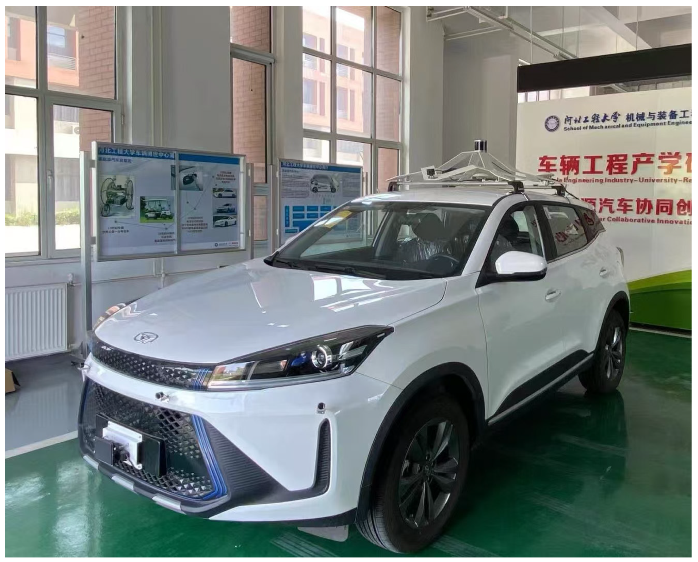
The vehicle platform of this experiment is equipped with rs-hellos-5s15 C32 line LiDAR (Shenzhen Suteng Juchuang Technology Co., Ltd., Shenzhen, China), IMU, and MiWen ape xad10 embedded artificial intelligence computer (China Wuxi Miwen Power Technology Co., Ltd., Wuxi, China) with NVIDIA Jetson AgX Orin processing unit. The software platform adopts the ROS (robot operating system) under the Ubuntu 20.04 operating system. The picture of the vehicle acquisition platform is shown in Figure 9.

Figure 9. This is the vehicle acquisition platform.

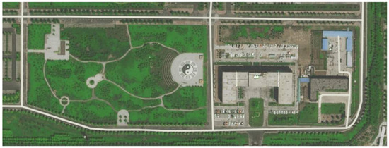
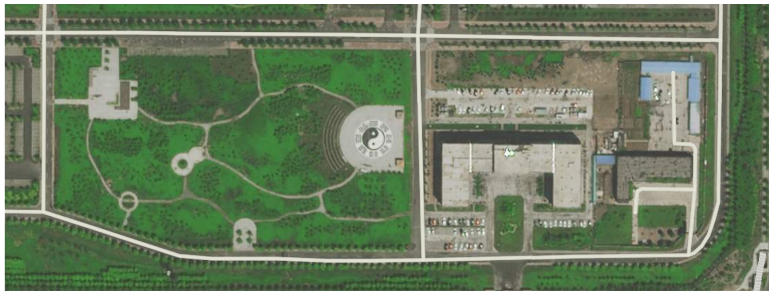
In this study, we selected a challenging open section within the campus for experimentation, as depicted in Figure 10. The environment of this section is complex, with dense vegetation on both sides and a variety of buildings surrounding it. In our experiments, we paid particular attention to the impact of the maximum vehicle speed on data accuracy. The experiments demonstrated that the algorithm can still function properly when the vehicle speed reaches 15 m/s.

Figure 10. This is a satellite map of the outdoor scene.

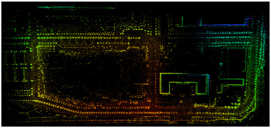
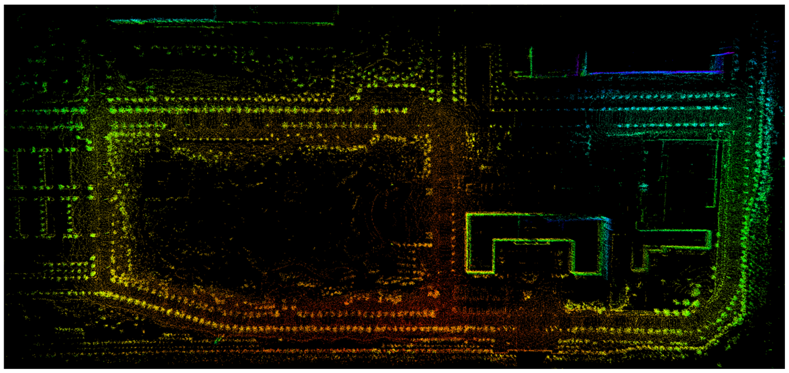
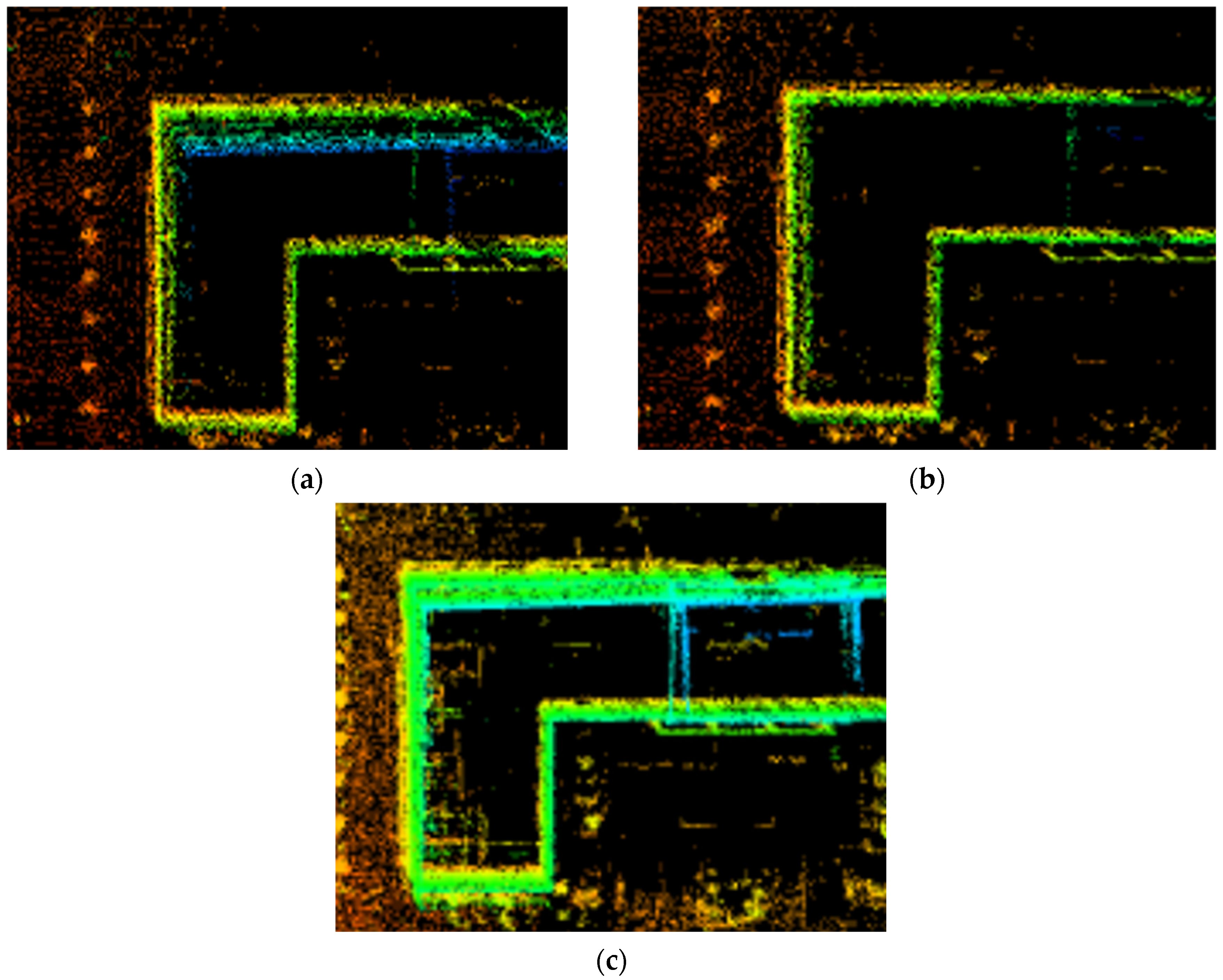
In order to ascertain the efficacy of our proposed algorithm, we utilized LIO-SAM and Point-LIO as benchmarks under uniform test conditions to perform trajectory localization and point cloud map generation on the identical road section. Figure 11 depicts the comprehensive map assembled by our algorithm. Additionally, Figure 12 offers a comparative analysis of the mapping efficacy between the aforementioned algorithms. A distinct observation from this comparison is the pronounced localization drift experienced by both LIO-SAM and Point-LIO, particularly at corner junctions. In contrast, our proposed algorithm effectively reduced cumulative errors, thereby eliminating drift phenomena during the map construction process.

Figure 11. This figure is the graph of the algorithm in this paper.

Figure 12. (a) A detailed comparison diagram of the LIO-SAM algorithm, (b) the algorithm in this paper, and (c) the Point-LIO algorithm.

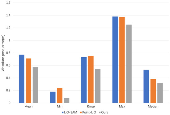
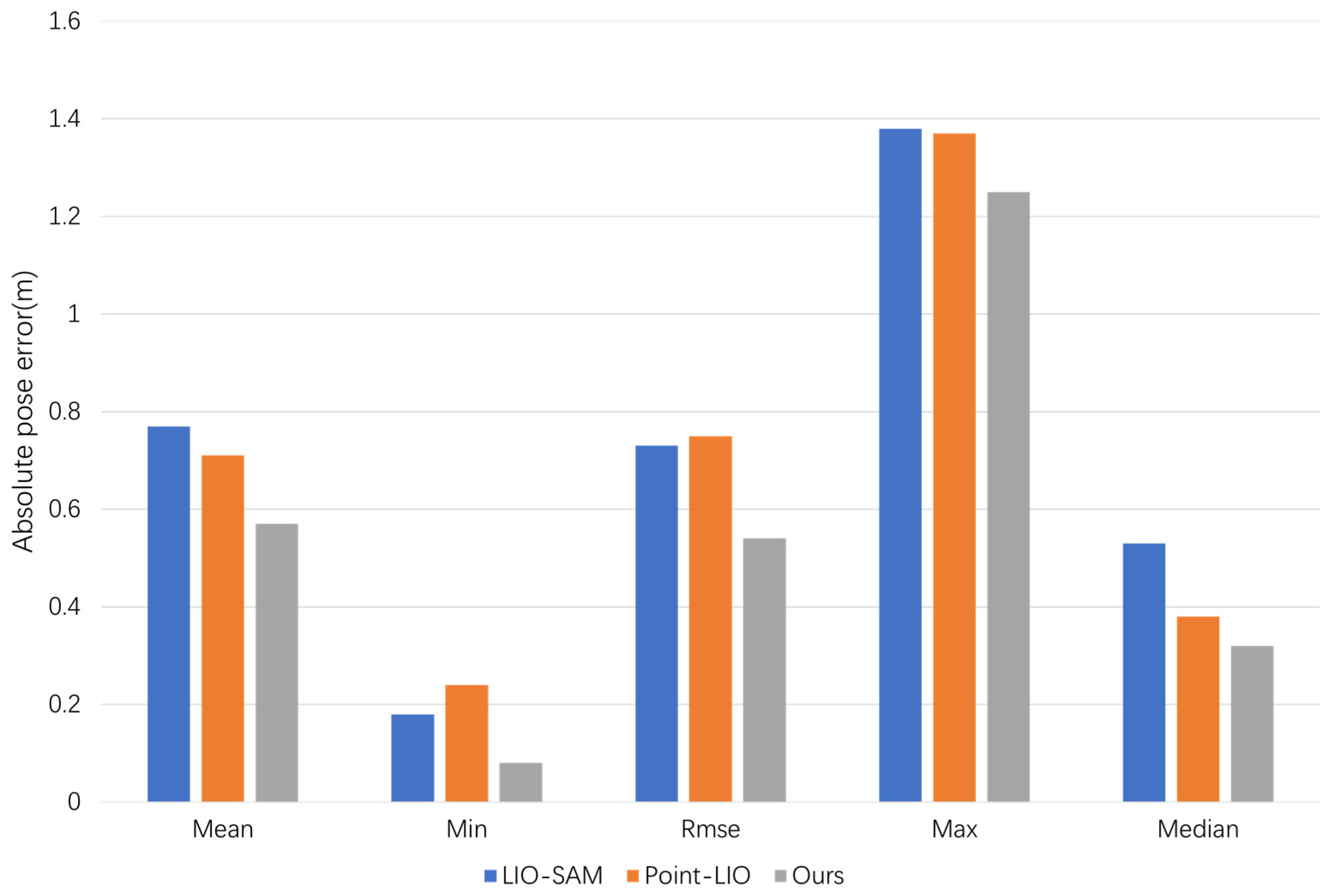
To validate the map-building accuracy of our algorithm in this study, we employed GPS signals as the benchmark truth for the trajectory and conducted an absolute trajectory error analysis of the mapping effects of both algorithms on an open outdoor section. The analysis results are shown in Figure 13. Through comparative analysis, it was found that the algorithm proposed in this paper is capable of achieving high-precision map construction in real outdoor open scenarios. Regarding absolute trajectory error, our algorithm realized a mean error of 0.57 m, markedly outperforming the LIO-SAM algorithm with an error of 0.76 m and the Point-LIO algorithm with an error of 0.71 m. In the context of maximum error, our approach surpassed the LIO-SAM and Point-LIO algorithms by 9.4% and 8.8%, respectively. With respect to median error, our algorithm, at 0.32 m, demonstrated superior performance compared to the LIO-SAM algorithm’s 0.53 m and the Point-LIO algorithm’s 0.38 m. Furthermore, our algorithm also held certain advantages in terms of minimum error and root mean square error.

Figure 13. The figure shows a comparison of trajectory errors between the three algorithms.

5. Conclusions

This paper presents a feature-optimized, tightly coupled Simultaneous Localization and Mapping (SLAM) algorithm aimed at overcoming the shortcomings of existing methodologies, thereby enhancing the positioning accuracy and robustness of autonomous vehicles. The proposed algorithm integrates an Inertial Measurement Unit (IMU) odometry module with a LiDAR odometry module through a tightly coupled framework, utilizing curvature feature optimization for improved feature extraction. This integration significantly enhances the accuracy and robustness of frame-to-frame matching. Experimental evaluations indicate that the algorithm demonstrates commendable performance on the KITTI dataset as well as in real-world applications, effectively reducing substantial localization errors and inaccuracies in map construction that are prevalent in conventional laser SLAM algorithms. While the fusion of IMU data and LiDAR point cloud data increases the computational demands relative to traditional laser SLAM approaches, the algorithm employs a local keyframe sliding window technique to mitigate real-time computational burdens and enhance efficiency. However, it is acknowledged that system overload may still arise in complex, high-speed environments. Future research will concentrate on further optimizing and refining the algorithm to achieve superior performance in practical applications, as well as investigating advanced sensor data processing techniques to contribute to the advancement of autonomous driving technology.

References

- Smith, R.C.; Cheeseman, P. On the representation and estimation of spatial uncertainty. Int. J. Robot. Res. 1986, 5, 56–68. [Google Scholar] [CrossRef] [Scilit]
- Mokssit, S.; Licea, D.B.; Guermah, B.; Ghogho, M. Deep Learning Techniques for Visual SLAM: A Survey. IEEE Access 2023, 11, 20026–20050. [Google Scholar] [CrossRef] [Scilit]
- Tee, Y.K.; Han, Y.C. Lidar-based 2D SLAM for mobile robot in an indoor environment: A review. In Proceedings of the International Conference on Green Energy, Computing and Sustainable Technology (GECOST), Miri, Malaysia, 7–9 July 2021; IEEE: Piscataway, NJ, USA, 2021; pp. 1–7. [Google Scholar]
- Montemerlo, M.; Thrun, S.; Koller, D.; Wegbreit, B. FastSLAM: A factored solution to the simultaneous localization and mapping problem. In Proceedings of the Eighteenth National Conference on Artificial Intelligence, Menlo Park, CA, USA, 28 July–1 August 2002; p. 593598. [Google Scholar]
- Zhao, S.; Zhang, H.; Wang, P.; Nogueira, L.; Scherer, S. Super odometry: IMU-centric LiDAR-visual-inertial estimator for challenging environments. In Proceedings of the IEEE/RSJ International Conference on Intelligent Robots and Systems (IROS), Prague, Czech Republic, 27 September–1 October 2021; IEEE: Piscataway, NJ, USA, 2021; pp. 8729–8736. [Google Scholar]
- Hess, W.; Kohler, D.; Rapp, H.; Andor, D. Real-time loop closure in 2D LIDAR SLAM. In Proceedings of the 2016 IEEE International Conference on Robotics and Automation (ICRA), Stockholm, Sweden, 16–20 May 2016; IEEE: Piscataway, NJ, USA, 2016; pp. 1271–1278. [Google Scholar]
- Bekrar, A.; Kacem, I.; Chu, C.; Sadfi, C. A branch and bound algorithm for solving the 2D strip packing problem. In Proceedings of the International Conference on Service Systems and Service Management, Troyes, France, 25–27 October 2006; IEEE: Piscataway, NJ, USA, 2006; Volume 2, pp. 940–946. [Google Scholar]
- Zhang, J.; Singh, S. LOAM: Lidar odometry and mapping in real-time. Robot. Sci. Syst. 2014, 2, 1–9. [Google Scholar]
- Rusinkiewicz, S.; Levoy, M. Efficient variants of the ICP algorithm. In Proceedings of the third international conference on 3-D digital imaging and modeling, Quebec City, QC, Canada, 28 May–1 June 2001; IEEE: Piscataway, NJ, USA, 2001; pp. 145–152. [Google Scholar]
- Low, K.L. Linear Least-Squares Optimization for Point-to-Plane Icp Surface Registration; University of North Carolina: Chapel Hill, NC, USA, 2004; Volume 4, pp. 1–3. [Google Scholar]
- Serafin, J.; Grisetti, G. NICP: Dense normal based point cloud registration. In Proceedings of the IEEE/RSJ International Conference on Intelligent Robots and Systems (IROS), Hamburg, Germany, 28 September–2 October 2015; IEEE: Piscataway, NJ, USA, 2015; pp. 742–749. [Google Scholar]
- Deschaud, J.E. IMLS-SLAM: Scan-to-model matching based on 3D data. In Proceedings of the IEEE International Conference on Robotics and Automation (ICRA), Brisbane, QLD, Australia, 21–25 May 2018; IEEE: Piscataway, NJ, USA, 2018; pp. 2480–2485. [Google Scholar]
- Segal, A.; Haehnel, D.; Thrun, S. Generalized-icp. Robot. Sci. Syst. 2009, 2, 435. [Google Scholar]
- Koide, K.; Yokozuka, M.; Oishi, S.; Banno, A. Voxelized GICP for fast and accurate 3D point cloud registration. In Proceedings of the IEEE International Conference on Robotics and Automation (ICRA), Xi’an, China, 30 May–5 June 2021; IEEE: Piscataway, NJ, USA, 2021; pp. 11054–11059. [Google Scholar]
- Shan, T.; Englot, B. Lego-loam: Lightweight and ground-optimized lidar odometry and mapping on variable terrain. In Proceedings of the IEEE/RSJ International Conference on Intelligent Robots and Systems (IROS), Madrid, Spain, 1–5 October 2018; IEEE: Piscataway, NJ, USA, 2018; pp. 4758–4765. [Google Scholar]
- Ye, H.; Chen, Y.; Liu, M. Tightly coupled 3d lidar inertial odometry and mapping. In Proceedings of the International Conference on Robotics and Automation (ICRA), Montreal, QC, Canada, 20–24 May 2019; IEEE: Piscataway, NJ, USA, 2019. [Google Scholar]
- Xu, W.; Zhang, F. Fast-lio: A fast, robust lidar-inertial odometry package by tightly-coupled iterated kalman filter. IEEE Robot. Autom. Lett. 2021, 6, 3317–3324. [Google Scholar] [CrossRef] [Scilit]
- Xu, W.; Cai, Y.; He, D.; Lin, J.; Zhang, F. Fast-lio2: Fast direct lidar-inertial odometry. IEEE Trans. Robot. 2022, 38, 2053–2073. [Google Scholar] [CrossRef] [Scilit]
- Cai, Y.; Xu, W.; Zhang, F. ikd-tree: An incremental kd tree for robotic applications. arXiv 2021, arXiv:2102.10808. [Google Scholar]
- Bai, C.; Xiao, T.; Chen, Y.; Wang, H.; Zhang, F.; Gao, X. Faster-LIO: Lightweight tightly coupled LiDAR-inertial odometry using parallel sparse incremental voxels. IEEE Robot. Autom. Lett. 2022, 7, 4861–4868. [Google Scholar] [CrossRef] [Scilit]
- He, D.; Xu, W.; Chen, N.; Kong, F.; Yuan, C.; Zhang, F. Point-LIO: Robust High-Bandwidth Light Detection and Ranging Inertial Odometry. Adv. Intell. Syst. 2023, 5, 2200459. [Google Scholar] [CrossRef] [Scilit]
- Wang, G.; Wu, X.; Jiang, S.; Liu, Z.; Wang, H. Efficient 3d deep lidar odometry. IEEE Trans. Pattern Anal. Mach. Intell. 2022, 45, 5749–5765. [Google Scholar] [CrossRef] [Scilit] [PubMed]
- Forster, C.; Carlone, L.; Dellaert, F.; Scaramuzza, D. On-manifold preintegration for real-time visual--inertial odometry. IEEE Trans. Robot. 2016, 33, 1–21. [Google Scholar] [CrossRef] [Scilit]
- Zhang, J.; Singh, S. Low-drift and real-time lidar odometry and mapping. Auton. Robot. 2017, 41, 401–416. [Google Scholar] [CrossRef] [Scilit]
- Shan, T.; Englot, B.; Meyers, D.; Wang, W.; Ratti, C.; Rus, D. Lio-sam: Tightly-coupled lidar inertial odometry via smoothing and mapping. In Proceedings of the IEEE/RSJ international conference on intelligent robots and systems (IROS), Las Vegas, NV, USA, 24 October 2020–24 January 2021; IEEE: Piscataway, NJ, USA, 2021; pp. 5135–5142. [Google Scholar]
- Quigley, M.; Conley, K.; Gerkey, B.; Faust, J.; Foote, T.; Leibs, J.; Berger, E.; Wheeler, R.; Ng, A.Y. ROS: An open-source Robot Operating System. In Proceedings of the ICRA Workshop on Open Source Software, Kobe, Japan, 12–17 May 2009; Volume 3, p. 5. [Google Scholar]
- Choi, S.; Zhou, Q.Y.; Koltun, V. Vladlen Koltun. Robust reconstruction of indoor scenes. In Proceedings of the IEEE Conference on Computer Vision and Pattern Recognition, Boston, MA, USA, 7–12 June 2015. [Google Scholar]
Disclaimer/Publisher’s Note: The statements, opinions and data contained in all publications are solely those of the individual author(s) and contributor(s) and not of MDPI and/or the editor(s). MDPI and/or the editor(s) disclaim responsibility for any injury to people or property resulting from any ideas, methods, instructions or products referred to in the content. |
© 2024 by the authors. Published by MDPI on behalf of the World Electric Vehicle Association. Licensee MDPI, Basel, Switzerland. This article is an open access article distributed under the terms and conditions of the Creative Commons Attribution (CC BY) license (https://creativecommons.org/licenses/by/4.0/).