


Abstract
Addressing the high-dimensional, strongly constrained multi-objective optimization problem of air–ground collaborative jamming scheduling in complex terrain, existing methods are often limited by incomplete modeling and low optimization efficiency in discrete feasible regions. This paper proposes a Terrain-Aware Multi-Scale Discrete Operator (TA-MSDO). A joint optimization model integrating discrete terrain characteristics and practical combat constraints is first constructed. Then, by leveraging the topological adjacency of terrain units, TA-MSDO employs a block-level crossover and a multi-scale mutation mechanism, replacing traditional continuous genetic operations to enable efficient and directional exploration of the discrete feasible region. Integrating TA-MSDO into the NSGA-III framework yields the enhanced ENSGA3 algorithm. Experimental results in a typical hilly terrain scenario demonstrate that ENSGA3 achieves a statistically significant performance improvement over the decomposition-based MOEA/D algorithm in terms of maximum achievable suppression effectiveness and hypervolume. As a comprehensive metric integrating convergence and Pareto frontier coverage, hypervolume further verifies the superior comprehensive optimization capability of the proposed algorithm. Meanwhile, compared with other classic mainstream multi-objective optimization algorithms including NSGA-II, standard NSGA-III and SPEA2, the proposed algorithm exhibits clear positive advantages in the upper bound of suppression effectiveness for elite solutions and operational stability across random initializations, with a favorable trend in Pareto frontier coverage for multi-objective collaborative optimization. This work provides an effective solution for jamming resource scheduling in complex battlefield environments.
1. Introduction
Currently, high-power jamming remains the primary method for interfering with inter-user communications at the physical layer [1]. While this approach exhibits certain effectiveness, it fails to meet the requirement for precise jamming in future operational scenarios. In the complex electromagnetic environment of informationized battlefields, multi-jammer systems based on cooperative control have been widely adopted [2]. In line with the development trend of cooperative systems, research on jamming resource scheduling has made progress. However, relevant studies still focus primarily on the field of radar countermeasures. Key decision variables in these optimization models typically center on power allocation [3,4,5,6,7], jamming waveforms [8], and frequency bands [9,10]. In contrast, research on resource scheduling specifically for communication jamming is extremely scarce.
The miniaturization of electronic devices is the core factor driving this evolution, enabling the deployment of compact, multi-functional jamming platforms. This technological advancement has laid the foundation for the development of air–ground cooperative integrated systems. Against this backdrop, air–ground cooperative distributed communication jamming resource scheduling has emerged as a transformative technical approach. Its core concept is to integrate scattered, miniaturized ground and airborne jamming platforms into a unified distributed system. By cooperatively scheduling multi-dimensional resources including the type of air–ground jamming platform [11], jamming mode [12], spatial deployment [13], and power [14], the system can effectively suppress various communication targets while significantly enhancing the concealment, robustness, and resource utilization efficiency of the entire jamming system.
Mechanistically, compared with traditional single-platform independent jamming, distributed jamming resource scheduling technology coordinates multiple spatially dispersed jammers to more efficiently integrate multi-dimensional resources, e.g., space, frequency, and power of jamming devices, with different locations and characteristics. This substantially increases the system’s flexibility in dynamic jamming parameter configuration and cooperative strategy selection. However, while this multi-platform, multi-dimensional resource scheduling mode offers significant advantages, it also introduces multiple technical challenges. First, due to the need to coordinate the synergy of multi-platform space, time, and frequency resources, the system’s decision space has expanded from the traditional low-dimensional convex solution space to a high-dimensional non-convex complex solution space, greatly increasing the solution complexity of scheduling strategies [15]. On one hand, the heterogeneous characteristics of fixed ground jamming equipment and airborne jamming equipment further exacerbate scheduling difficulties; on the other hand, the strong coupling between multi-platform resources means that adjustments to any dimension of resources require linkage with other dimensions, and isolated modeling cannot accurately characterize their inherent correlation laws.
Current research methods for resource scheduling mainly include game theory [16,17], swarm intelligence algorithms [18,19,20], and deep reinforcement learning (DRL) [21,22,23,24,25]. Although DRL shows potential in solving resource scheduling problems in specific dimensions such as resource allocation, it has certain limitations in model design and methodology when addressing the highly complex scenario of air–ground cooperative distributed communication jamming resource scheduling mentioned above.
For the highly complex scenario of the aforementioned distributed jamming resource scheduling, existing research is mostly concentrated in the radar countermeasure domain, while dedicated scheduling studies targeting wireless communication jamming remain relatively scarce. Existing methods often directly borrow models and frameworks (e.g., deep reinforcement learning) from the radar domain, yet they have significant limitations in model design and methodology: first, they generally rely on idealized assumptions, ignoring platform heterogeneity [26] and the physical coupling between jamming deployment and electromagnetic propagation [27]; second, they insufficiently model complex terrain occlusion and geographic constraints [28], resulting in poor generalization capability of strategies in real-world environments; third, facing the high-dimensional, non-convex, and strongly coupled decision space, DRL encounters challenges in exploration efficiency and reward design, making it difficult to stably converge to executable strategies.
In addition, the objective functions of existing models are relatively simplistic, often reduced to a trade-off between jamming effectiveness and energy consumption. Insufficient attention is paid to multi-dimensional operational metrics such as concealment and survivability, which makes it hard to reflect the advantages of distributed cooperative scheduling. Meanwhile, when traditional multi-objective evolutionary algorithms are applied to such discrete terrain-constrained problems, there is a mismatch between their standard continuous genetic operators and the structure of the discrete feasible domain, leading to low search efficiency.
To address the aforementioned issues, this study constructs a joint scheduling and deployment model for heterogeneous air–ground platforms, in which the hexagonal cellular grid is adopted to discretize complex terrain and the occlusion effect of terrain on electromagnetic propagation is characterized; this model further incorporates practical engineering constraints, including terrain masking, platform heterogeneity, multi-dimensional resource coupling, co-frequency spacing, and exposure risk, thereby transforming the communication interference scheduling problem into a high-dimensional, discrete, and highly constrained multi-objective optimization task, which typically exhibits the core characteristics of “strong multi-objective conflicts, discrete combinatorial decision-making, and complex constraint coupling”: indicators such as suppression effect, deployment cost, resource consumption, and concealment are mutually restrictive, making it difficult to be fully represented by a single weighted objective; decision variables consist of discrete/integer variables, including candidate grid position indices, platform types, communication channels, and power levels, resulting in a complex combinatorial search space; additionally, constrained by forbidden grids, occupancy conflicts, minimum co-frequency spacing and other constraints, the feasible region is often fragmented and strongly coupled; furthermore, metrics such as suppression rate are typically formed through threshold judgment and counting ratio, leading to an objective landscape with non-smoothness and “step effect”, where performance improvement relies on structural restructuring rather than continuous micro-perturbations.
Given this problem structure, this study selects the Non-dominated Sorting Genetic Algorithm III (NSGA-III) as the solution framework, primarily due to its suitability for many-objective optimization scenarios. NSGA-III extends the classic framework of NSGA-II, driving the population toward the Pareto front through mechanisms of non-dominated sorting and elitist preservation. In contrast, the crowding distance metric used in NSGA-II tends to lose its discriminatory power as the number of objectives increases, often resulting in solutions that cluster in specific regions or exhibit insufficient coverage of the Pareto front. NSGA-III addresses this limitation by introducing a more stable distribution control mechanism based on a set of uniformly distributed reference points/directions. This approach explicitly maintains the coverage and uniformity of the solution set in the multi-objective space, making the algorithm more inclined to produce a diverse set of non-dominated candidate solutions that cover various trade-off preferences, rather than just a few concentrated compromise points. This characteristic aligns well with the requirements of engineering tasks such as jammer deployment and parameter configuration, where “a portfolio of solutions, not a single-point answer” is often needed. Furthermore, the global environmental selection and elitist preservation mechanisms in NSGA-III help to consistently retain candidate solutions with significantly different structures within the discrete and fragmented feasible region. This reduces the risk of premature convergence and homogenization while providing more substantial search support for the structural leaps required to overcome threshold-based “step effects” in the objective landscape.
Building upon this foundation, this study proposes a Terrain-Aware Multi-Scale Discrete Operator (TA-MSDO) to overcome the limitations of the traditional “continuous-generation and discrete-projection” paradigm. TA-MSDO introduces a block-level crossover based on topological adjacency and multi-scale mutation: the block-level crossover aims to maintain the configuration integrity of solutions across dimensions such as location, platform type, channel, and power; the multi-scale mutation integrates local refinement and global perturbation to fully exploit the topological structure of the discrete feasible region, thereby enhancing search efficiency. Furthermore, we embed TA-MSDO into the NSGA-III framework and combine it with Latin Hypercube Sampling to enhance population initialization, constructing an Enhanced Multi-objective Algorithm (ENSGA3). This significantly improves search efficiency and solution set quality under high-dimensional constraints. Concurrently, this study establishes a multi-objective collaborative framework encompassing jamming effectiveness, deployment cost, resource consumption, and stealthiness. Through normalization and comprehensive optimization, effective trade-offs among these heterogeneous objectives are achieved, better aligning with practical operational requirements. In summary, by integrating the strengths of NSGA-III in maintaining multi-objective distribution with the structural adaptability of TA-MSDO in discrete space search, this work provides an efficient and practical solution for air–ground cooperative jamming scheduling in complex terrain.
2. System Model
2.1. Digital Terrain Model
This paper considers a 25 km × 25 km area based on actual terrain, which can be regarded as a typical hilly terrain. The absolute elevation z (in meters) is used to describe the terrain and antenna height. The elevation in the area ranges from approximately 10 m to 280 m, covering low-altitude plains, gentle hills and plateaus, and local low mountains. This terrain includes both near-line-of-sight flat paths and multi-scale protrusions and depressions, making it suitable for verifying channel models that integrate the combined effects of diffraction, shadowing, and multi-point jamming. To balance computational complexity and physical fidelity, this paper discretizes the continuous terrain into a regular hexagonal honeycomb grid. The entire area is divided into 16 × 16 hexagonal cells, totaling 256 cells, forming an elevation grid . The center-to-center distance of each cell is approximately 1 km, whose geometric size is much larger than the operating wavelength and also significantly larger than the typical radius of the first Fresnel zone [29]. Thus, each honeycomb cell can be regarded as an equivalent terrain block with approximately constant local elevation in the electromagnetic sense.
For each hexagonal cell:
Herein, denotes the planar coordinates of the cell center, with the unit of km; represents the representative elevation of this cell; and refers to the geometric coverage area of the cell, i.e., the set of all points on the plane that belong to this cell.
Cells are categorized into four types based on elevation: plain, low hill, high hill, and mountain. Meanwhile, this paper further discretizes the interior of each honeycomb cell into six uniformly distributed candidate nodes. These candidate nodes are symmetrically distributed within the cell plane; their planar coordinates are determined by the cell center coordinates, and they inherit the elevation attribute of the cell they belong to. Each candidate node remains affiliated with its host cell and shares the terrain category and elevation value of that cell. This two-level discretization design (cell and sub-node) maintains the constraint characteristics of terrain blocks at the macro level, while providing a sub-kilometer adjustment space for jammer deployment at the micro level—thus better aligning with the practical engineering requirement that equipment can flexibly select locations within a small local range.
For any point on the plane, its affiliated cell is defined as
Then, the terrain elevation of this point is
As shown in Figure 1 below:
Figure 1.
Terrain Model Diagram.
2.2. Channel Loss Model
To accurately evaluate the communication link quality in the air–ground cooperative network, this paper establishes a channel model that comprehensively considers free-space propagation loss, terrain occlusion and diffraction effects, and electromagnetic environment countermeasures. This model simulates discrete terrain data and is applicable to tactical communication scenarios in the UHF frequency band.
The total path loss is expressed as
where denotes the free-space propagation loss, denotes the diffraction loss, and represents the loss caused by other factors such as the electromagnetic environment and equipment characteristics; all are in units of dB.
2.2.1. Free-Space Propagation Loss
The free-space path loss describes the attenuation of electromagnetic waves in an ideal environment without obstacles or multipath reflection, which is mainly caused by spherical wave spreading. According to the Friis transmission formula [30], the standard free-space loss is calculated as
where d is the distance between the transmitter and the receiver (in km), and f is the carrier frequency. The coordinates of the transmitter are , and the coordinates of the receiver are ; the 3D Euclidean distance is expressed as
Here, z denotes the sum of the elevation height and the antenna transmission height.
2.2.2. Channel Modeling
Depending on the type of endpoints (ground nodes or aerial nodes) in the communication link, the propagation characteristics of electromagnetic waves vary significantly. This paper classifies the links into air-to-air (A2A) links, air-to-ground (A2G) links, and ground-to-ground (G2G) propagation links;
- A2A: A2A link refers to a communication link where both the transmitter and receiver are aerial nodes. Since both parties are located at relatively high altitudes (typically h ≥ 2000 m), the propagation path is usually unobstructed by ground terrain and can be regarded as free-space propagation. Therefore, A2A links operate under line-of-sight (LoS) propagation, so the path loss of A2A links in this paper is defined as
- A2G: A2G link refers to a link where one end is an aerial device and the other is a ground device. Although ground nodes may be affected by terrain, the following factors support the line-of-sight (LoS) assumption for A2G links: A2G and G2A links are still likely to be macroscopically LoS, but they differ from A2A links: the propagation environment near the ground end is significantly more complex, leading to a systematic reduction in the average received power compared to pure FSPL predictions. This is mainly reflected in the fact that even if the link is geometrically LoS overall, terrain undulations, ridges, and local protrusions at the ground-proximal end make the direct line-of-sight more prone to obstruction near the ground; meanwhile, surface reflection and scattering around the ground end are significantly stronger than in high-altitude free space. Even when LoS still dominates, fluctuations and average additional attenuation caused by spatial or surface scattering will occur. After comprehensive consideration, the nonexplicitly modeled but prevalent non-ideal factors are combined into = 12 dB. Given that the occlusion of A2G links is mainly controlled by the terrain at the ground-proximal end, while the high-altitude path segment far from the ground approximates free space, this paper only uses the knife-edge diffraction model presented below to calculate the ground-proximal end loss for the path proportion = 0.3 near the ground end, where terrain occlusion is highly uncertain. To address this uncertainty, a protective upper limit of 14 dB is set based on the 12 dB baseline model, in order to enhance robustness in real-world environments, thus deriving the A2G link loss model:
- G2G: G2G link refers to a transmission link where both ends are ground-based devices. Since both parties are located on the terrain surface, the terrain occlusion effect is significant, and the transmission path between ground devices is fully exposed to terrain influences. Even in relatively flat terrain, small-scale undulations may cause issues such as partial occlusion of the Fresnel zone and terrain diffraction loss; the loss is expressed as
Herein, denotes the horizontal distance (in meters), and N is the number of sampling points. The sampling coordinates of any point are given by
For each sampling point , the corresponding ground elevation is queried from the terrain database. The sampling interval of the terrain profile should be moderate to balance accuracy and computational efficiency. In this paper, is selected, which can capture the characteristics of typical terrain undulations (the terrain grid resolution in this study is 1.54 km) and is sufficient to describe the terrain profile accurately.
Normalized Line-of-Sight Parameter:
where t = 0 corresponds to the transmitter end, and t = 1 corresponds to the receiver end.
LoS Line Height at Arbitrary Position t:
For each terrain cell, determine the ray crossing range by collecting all t-values corresponding to the sampling points that fall within the cell:
Calculate the entry and exit positions in any honeycomb region:
Calculate the LoS line height:
Obstacle Determination Condition:
In the simulation of terrain profile modeling, the minimum height of the LoS within the terrain cell is used as the critical threshold for obstacle determination:
Its theoretical basis is as follows: The height of the LoS along the path within the cell varies linearly, and its minimum height is located at the point where the LoS is closest to the terrain. If the terrain height , there must be occlusion within the cell; conversely, if , the LoS remains unobstructed throughout. The terrain in this paper is simulated by discrete sampling, and the terrain elevation is provided by a discrete digital elevation model with limited data point density. Using can avoid sampling errors and prevent misjudgments caused by single-point terrain fluctuations.
Critical Position Selection:
The endpoint with the lower LoS height is selected as the reference position for diffraction calculation:
Effective Obstacle Height:
Distance from the obstacle to the transmitter and receiver:
First Fresnel Radius :
Diffraction Loss Calculation, Fresnel–Kirchhoff Diffraction Parameter v:
Equation (22) is mainly used to calculate the Fresnel–Kirchhoff diffraction parameter ν, while Equation (23) is a diffraction loss model established based on the ITU-R P.526 specification. It specifically presents the functional relationship between the knife-edge diffraction loss caused by a single obstacle and the diffraction parameter ν.
Diffraction Loss Model Based on ITU-R P.526 Specification:
The knife-edge diffraction loss for a single obstacle is
Multi-Obstacle Coupling:
The dominant propagation loss comes from 1–2 key obstacles. We retain the two obstacles with the largest v values for subsequent calculations. The rationality of this selection is supported by standards, physics and empirical evidence. It aligns with ITU-R P.526, which indicates that multi-knife-edge diffraction loss is dominated by the most significant obstacle; the third and subsequent obstacles contribute little and can be ignored in the shadow fading scenario. When two obstacles are close, the diffraction field of the main obstacle distorts the field at the secondary one and reduces its effective occlusion. This nonlinear superposition is considered. Based on massive electromagnetic simulations and experimental data, the coupling coefficient is defined as
When , the two cells are very close: the diffraction field of the main obstacle has diverged significantly at the secondary obstacle, so the secondary obstacle only interacts with the attenuated diffraction field, and the effective occlusion is halved. When the distance is relatively large, the two obstacles act independently on the direct wave, with no significant coupling. The weighted sum of the total diffraction loss is
Hexagonal honeycomb discretization is applied to the terrain so that the continuous and complex surface is partitioned into uniformly sized hexagonal cells. The elevation of each cell is defined as the maximum terrain height within its coverage area, and the cell top is treated as an equivalent knife-edge obstacle. This discretization is a conventional engineering approach in terrain-based wireless propagation analysis and provides more uniform spatial distribution than square grids, leading to a path sampling error no greater than 4% [31]. It therefore enables the continuous terrain profile to be decomposed into discrete obstacle units that can be analyzed independently along a link. This design is consistent with the core assumption of ITU R P.526 [30], where diffraction is modeled by knife-edge structures and the dominant factor is the vertex height responsible for occlusion rather than detailed slope geometry. Based on this discretized representation, the propagation evaluation follows a simplified ITU R P.526 knife-edge diffraction formulation with terrain profile sampling. For each transmitter receiver link, the terrain elevation is sampled along the path at a fixed spatial interval, the nearest honeycomb cell is queried at each sample point, and diffraction loss is computed using Fresnel parameter-based knife-edge attenuation, including obstacle coupling for ground-to-ground links and a reduced near-ground diffraction treatment for air-to -ground links. As a result, the cost of a single link evaluation grows with both the number of profile samples and the terrain query workload, and each candidate deployment evaluation requires many such link computations, making the overall optimization runtime dominated by repeated terrain-aware propagation calculations.
2.3. Countermeasure Scenarios and Decision Model Construction
2.3.1. Scenario Overview
In this scenario, the communicating party uses Frequency Division Multiple Access (FDMA) to divide the communication network into three mutually orthogonal working channels, denoted as . The set of communication nodes is N, and each communication node is fixedly bound to one channel . Each channel contains multiple communication nodes in this scenario: the superposition relationship between useful signals and interference only occurs between co-frequency entities, while inter-frequency entities have no mutual influence in the model. Time Division Multiple Access (TDMA) is adopted within the same carrier frequency f. Let represent the set of directed service links in the active state on carrier frequency f at time t: . Therefore, only one service transmitter and one service receiver exist on the same carrier frequency at any time. This concurrent structure is used to define the instantaneous service form at the receiving moment. Given the propagation environment and path loss model, the path loss from any transmitter a to receiver b on carrier frequency f is . Let the transmit power be and the antenna gains of the transmitter and receiver be and , respectively. The received power is defined as
The set of jammers is denoted as . The deployment decision for each jammer is recorded as
where is the candidate location index; is the platform type; is the jamming frequency; is the discrete power level. The overall scheme is . Let the set of hexagons be C and the set of candidate points be . For a candidate point , its coordinates are , and it belongs to the elevation region . Given the set of forbidden area grids , the constraint is .
Mutual Exclusion Constraint
Only one jammer can be deployed in each elevation region:
To avoid strongly correlated radiation, short-range mutual coupling, and coverage redundancy caused by excessive spatial aggregation of co-frequency jammers while reducing the risk of being located by the opponent, this study imposes a minimum spacing constraint on jammers operating on the same carrier frequency, to prevent tactically unreasonable co-frequency concentrated stacking deployment:
To exclude extreme near-field deployments that lack engineering feasibility or tactical significance, we further set the restriction that the maximum arrival power generated by any jammer on its operating carrier frequency to any communication node shall not exceed a preset threshold. The purpose of this constraint is to avoid non-far-field propagation conditions caused by overly short distances that reflect concealment and risk control requirements; excessively strong arrival power usually implies a high exposure probability and greater vulnerability to countermeasures in practice. Therefore, this threshold constraint limits the space to a reasonable range that is modellable, implementable, and evaluable for countermeasures, making the resulting deployment scheme more practically solvable and reproducible in experiments:
For any communication node whose associated carrier frequency is f, define the set of co-frequency potential transmitting nodes as . For any , the communication received power is expressed as
Define the key link signal strength of the estimated node n as
This represents the estimated useful signal strength obtained by node n at its receiving moment.
2.3.2. Interference Superposition and Suppression Determination
For any communication node n, its co-frequency jammer set is , . Let the transmit power of the jammer be , , and the transmit-side gain be ; the arrival power of a single jammer (in dBm) is defined as
Co-frequency total interference is superposed in the power domain:
Define the Jammer-to-Signal Ratio (JSR) at the receiving moment as
Given a threshold , the suppression target is defined as
And the network-wide suppression rate is defined as
2.4. Construction of Multi-Objective Optimization Model
The decision-making of jammer deployment is essentially a trade-off between effectiveness and risk: under engineering constraints, e.g., given the number of jammers, forbidden areas, mutual exclusion, spacing, and upper limit of arrival power, the choices of deployment location, platform type, operating frequency, and power level will simultaneously affect suppression coverage, platform investment, energy/resource consumption, and the probability of being detected by the opponent. Pursuing only the single objective of suppression rate often leads to extreme schemes, e.g., high-power, short-distance, more aerial platforms—though suppression is strong, the cost and exposure are unacceptable. Conversely, pursuing only concealment or energy conservation may fail to meet the suppression threshold. Therefore, this paper adopts multi-objective optimization, decomposing the key requirements of jammer deployment into the following four categories, which are simultaneously optimized within the same framework. For any deployment scheme, .
- Suppression Effectiveness
At the task level, the primary concern is how many targets can be suppressed. This paper uses the reception-time-oriented suppression rate to characterize the network-wide suppression coverage level: under a given JSR threshold, a higher proportion of suppressed nodes indicates stronger overall suppression effectiveness of the scheme. This objective directly corresponds to the primary effectiveness indicator of the countermeasure task. Denote the objective as
- 2.
- Deployment Cost Score
Jamming platforms typically incur higher acquisition, operational, and maintenance costs. On the premise of achievable suppression, reducing platform investment helps improve the usability and implementability of the scheme. The weight of deployment cost is set higher for ground platforms than for aerial ones—this reflects that ground platforms are subject to stronger constraints, e.g., terrain accessibility, camouflage, fortification construction, and support deployment, leading to higher occupation and deployment costs, while aerial platforms allow for relatively flexible mobile deployment. Therefore, a cost indicator composed of the number of platforms and their weights is introduced to characterize the deployment cost required to achieve the current suppression effectiveness. Let the number of aerial and ground jammers be and , respectively; the linear deployment cost is defined as
- 3.
- Resource Consumption
Transmit power and continuous radiation lead to issues such as energy consumption, equipment load, and mission sustainability; meanwhile, higher power typically increases the risk of detection. Therefore, an independent indicator is needed to characterize how much transmit resource is consumed to achieve the current suppression effectiveness, and to constrain schemes with excessively high power or resource occupancy. The weight of resource consumption is set higher for ground platforms than for aerial ones—this reflects that continuous high-power operation of ground platforms is more strongly constrained by operating conditions, and increasing power imposes a heavier support burden and greater sustainability penalty. Assume the power level index ranges over 10 levels. Let denote the maximum available power of platform type . For the power occupancy of each jammer, the platform resource weights for aerial and ground platforms, denoted as and , respectively, are introduced to define resource occupancy:
- 4.
- Concealment
In a countermeasure environment, the jamming party typically needs to avoid being localized and identified by the communication side or detection systems. The exposure risk is related to factors such as the interference intensity reaching the opponent’s nodes and spatial distance. The risk weight is set higher for aerial platforms than for ground platforms—this reflects that after electromagnetic radiation exposure, aerial platforms are more vulnerable to long-range detection and interception, have limited evasion space, and incur higher survivability costs. This objective is used to measure whether the deployment scheme can maintain low detectability and exposure level while achieving suppression, thereby improving survivability and sustainable operational capability. Let denote the communication detectability threshold and denote the strong exposure threshold. Let (in km) be the distance between jammer k and communication device n; the distance weight is defined as
Here, is the near-field distance threshold, and is the far-field distance threshold; is the far-field weight coefficient. For any jammer k, check if there is an excessively high power condition among all communication nodes: if the predicted received power for a certain node n, it is considered strongly exposed; otherwise, the average risk is calculated only for other nodes:
Here, and are the fixed exposure factors of aerial and ground platforms, respectively. On this basis, the overall exposure risk objective function is derived as
In jammer deployment optimization, in addition to suppression capability, the scheme should also perform better in engineering attributes such as deployment cost, resource consumption, and concealment. We construct a comprehensive effectiveness objective by multiplying the three utilities with the suppression rate, so that each objective is comparable in numerical scale. This indicates that it is meaningful only under the premise that the suppression task is effective: we regard the suppression rate as the effectiveness intensity of the scheme at the task level, while indicators such as cost, resource, and concealment describe the condition quality when the scheme is in operation. Therefore, the complete optimization objective is
To mitigate disparities in dimensions and scales across heterogeneous optimization objectives—as such inconsistencies can undermine the validity of subsequent optimization procedures—this paper employs normalization techniques for both the suppression rate and each individual term corresponding to the optimization objectives, mapping all such metrics onto the standardized unit interval [0, 1] during the modeling phase. The four optimization objectives are denoted as . Resource Efficiency (resEff): A positive indicator derived from the normalization of the “resource consumption” objective, ranging from [0, 1]. A higher resEff value indicates lower resource (power) consumption of jammers under the same suppression effect and higher resource utilization efficiency, which is calculated as the inverse mapping of the normalized resource consumption objective; Deployment Efficiency (deployEff): A positive indicator converted from the normalization of the “deployment cost” objective, ranging from [0, 1]. A higher deployEff value means lower platform deployment cost required to achieve the current suppression rate, with stronger deployment economy and implementability, obtained through the inverse normalization of the deployment cost objective; Stealth Efficiency (stealthEff): A normalized positive indicator corresponding to the “stealthiness” objective, ranging from [0, 1]. A higher stealthEff value represents lower exposure risk of jammer deployment and stronger stealth and survivability, derived from the inverse mapping of the normalized stealthiness objective.
When the suppression rate Suppr is kept fixed in the context of our resource scheduling optimization experiments, , , are strictly monotonically increasing with ; as long as the suppression rates are similar, the optimization algorithm will still prefer solutions with lower cost, less resource consumption, and better concealment, which will naturally lead to Pareto differentiation in these dimensions. When the suppression rate (Suppr) is low, the scheme is not automatically eliminated. Since follows a product structure, a low suppression rate can be partially offset by sufficiently high , so the scheme still remains competitive in the original dimensions and may enter the non-dominated set.
When constructing a multi-objective optimization model, it is crucial to accurately define the relevant symbols and their meanings. As shown in Table 1 “Multi-Objective Optimization Model: Symbols and Definitions”, this table comprehensively lists various symbols involved in the model along with their precise definitions. By referring to this table, we can clearly understand the physical or mathematical concepts represented by each symbol in the model, thus laying a solid foundation for the subsequent analysis and solution of the model. If a scheme produces almost no suppression effect, its engineering attributes—even if it is highly resource-efficient or extremely concealed—can hardly be converted into usable operational value. The multiplicative structure causes engineering benefits to naturally attenuate when the task is invalid, thereby preventing invalid solutions with high engineering scores from occupying a large number of non-dominated positions in the multi-objective sense and contaminating the Pareto front. The multi-objective optimization of jammer deployment faces two key challenges: the decision variables involve a four-dimensional discrete configuration of location, type, frequency, and power, and are subject to multiple spatial-spectrum coupling constraints, resulting in a highly fragmented feasible region; the objective function and constraint evaluation have characteristics such as piecewise thresholds and nonlinear superposition, showing discontinuous, non-differentiable, and multi-modal features, which leads to high computational overhead. Thus, this problem is NP-hard. This paper adopts a multi-objective evolutionary search framework based on the Pareto dominance relationship to obtain a high-quality trade-off solution set at an acceptable computational cost.
Table 1.
Multi-Objective Optimization Model: Symbols and Definitions.
3. Multi-Objective Optimization Method
3.1. Scenario Definition
Deployment of Communication Nodes
Aiming at the analysis of communication jamming mechanisms in complex mountainous terrain, this study proposes a systematic node deployment method under terrain constraints that constructs a controllable, interpretable, and engineering-practical simulation scenario for jamming modeling and performance evaluation. Existing node deployment methods are mostly random or uniform; while easy to implement, they fail to reflect the real situation of mountainous sites constrained by terrain and limited by constructible locations, resulting in a disconnect between simulation and practice.
To address this issue, this paper establishes a terrain-feature-constrained node deployment scheme based on hexagonal cellular terrain grids. First, a hexagonal terrain grid containing typical mountain massifs and hillocks is constructed, with each hexagonal cell serving as a potential site candidate area. Aerial equipment is deployed dispersedly in high-altitude and highland cells above multiple mountain massifs to form a cross-mountain coverage structure. Ground equipment is restricted to low-altitude, engineering-accessible areas, deployed in ring/band shapes along the periphery of mountain massifs, and forms complementary coverage with aerial equipment. Meanwhile, a non-deployment mechanism for adjacent cells is adopted to ensure the minimum geometric spacing between nodes, avoiding strong coupling interference caused by node aggregation, and thus guaranteeing the balance of coverage, jamming, and sampling. While maintaining analytical rigor, this scheme is close to real mountainous networks, provides typical link combinations for the analysis of jamming paths and diffraction effects, and can effectively support jamming modeling and performance evaluation for the analysis of communication jamming mechanisms in complex mountainous terrain.
The following is the logic of the node generation method, with key links defined as follows:
During available channel deployment, devices are divided into three groups by frequency, with four devices deployed in each group: one aerial communication node and three ground nodes. The link availability threshold is determined by sensitivity and margin: G2G links require a margin of at least 15 dB, while A2G links require a margin of at least 10 dB. Superimposing the link margin on the basis of sensitivity is equivalent to a conservative design for shadow fading, model errors, and engineering allowances. The higher margin for G2G links reflects stronger occlusion on the ground, while the lower margin for A2G links indicates that air-to-ground links are more stable.
The communication node information is shown in Table 2, and the communication node deployment is illustrated in Figure 2. Distance constraints are imposed on co-channel links to obtain the co-channel distance windows: the co-channel G2G distance window ranges from 4.2 km to 10 km, and the co-channel A2G distance window ranges from 5 km to 15 km. The lower limit avoids excessively short and strong links to reduce over-coverage and mitigate geometric degradation, while the upper limit prevents excessively long and weak links to improve the controllability of threshold compliance and ensure network availability. Furthermore, this constraint is only effective for co-channel links, which conforms to the engineering logic that co-channel interconnection and co-channel mutual interference are the most sensitive.
Table 2.
Communication node information.
Figure 2.
Communication Node Deployment Diagram.
After the deployment is completed, key receiving links are defined for each communication device, with 12 links in total; the purpose is to ensure link availability while providing targets for subsequent jamming optimization. In summary, this study adopts multi-layered rules including frequency grouping, elevation-guided deployment, co-channel distance window constraints, threshold margin restrictions, and adjacent forbidden zone isolation. These rules generate a benchmark scenario of communication nodes with engineering interpretability, link availability, and spatial rationality. Furthermore, a co-channel key receiving link is established for each device, providing a unified and reproducible experimental baseline for subsequent jamming resource optimization.
3.2. Initial Population Generation Based on Latin Hypercube Sampling
The coverage and structure of the initial population not only affect the convergence speed of the algorithm, but also influence the approximation accuracy and distribution uniformity of the final solution set to the true Pareto front. The standard implementation of NSGA-III usually adopts random sampling to construct the initial population. In the discrete strongly constrained problem studied in this paper, the feasible region is fragmented by multi-dimensional constraints. In the early iteration stage, pure random sampling may lead to the risk of population clustering and the problem of insufficient coverage of the feasible region. Therefore, this paper adopts Latin Hypercube Sampling (LHS) to optimize the initial population generation. Latin Hypercube Sampling can reduce the risk of population clustering caused by pure random sampling under the condition of limited samples.
This paper uses Latin Hypercube Sampling (LHS) instead of standard random initialization to generate the initial population of NSGA-III. The core idea of LHS is stratified sampling in each dimension of variables: divide the domain of the d-th dimension variable into N equal-probability intervals, and ensure each sub-interval is sampled exactly once in this dimension. This achieves approximately uniform coverage in the marginal distribution of each dimension, significantly reducing the clustering risk of pure random sampling under limited samples.
The decision vector is
Let be a random permutation of the set , and let be independent uniform random numbers. The continuous sampling of the i-th individual in the d-th dimension is
Since the decision variables in this paper are mainly integer-encoded, the continuous samples obtained by LHS need to be mapped to the integer value set. For interval-type integer variables, a consistent mapping combining rounding to the nearest integer and boundary clipping is adopted:
3.3. Terrain-Aware Multi-Scale Discrete Operator
The optimal deployment of distributed jammers is one of the key engineering problems to achieve efficient spectral suppression of enemy communication links while balancing own-side concealment and deployment costs. Targeting the collaborative tasks of multi-jammer platforms, this problem requires trade-offs among multiple objectives such as suppression effectiveness, concealment, resource consumption, and deployment costs, while satisfying the strict constraints derived from operational environments and platform collaboration mechanisms:
- The deployable positions of jammers are constrained by discrete terrain grids and candidate point sets, with decision variables exhibiting a topological structure defined by terrain adjacency in the spatial domain;
- Minimum electromagnetic spacing constraints must be satisfied between co-frequency jammers to avoid mutual interference and exposure risks;
- Discrete feasibility conditions including no-go cells, occupied cells and duplicate deployment further compress the feasible region.
NSGA-III is widely used in complex engineering optimization because its reference direction-guided non-dominated sorting and population selection mechanism can effectively balance convergence and the diversity of the Pareto front in multi-objective scenarios. However, in the jammer deployment problem under discrete terrain topology constraints, directly adopting continuous genetic operators such as Simulated Binary Crossover (SBX) and Polynomial Mutation (PM) usually requires projecting continuous offspring back to the integer domain via clipping and other methods. This process of continuous generation and discrete projection has an inherent incompatibility with the problem structure. On the one hand, continuous perturbations may be eliminated after quantization, leading to insufficient effective mutation and premature homogenization of the population; on the other hand, the numerical proximity of discrete variables such as candidate point indices does not equate to actual spatial proximity. The search hypothesis of continuous operators based on Euclidean interpolation fails to exploit terrain topology information, and is prone to generating topologically meaningless jumps or degrading into random perturbations. Meanwhile, under the combined effect of strict constraints and discrete feasibility conditions, continuous operators struggle to stably generate high-quality feasible solutions, thereby limiting the algorithm’s search efficiency, solution set quality, and statistical robustness.
Based on the above analysis, while keeping the main framework and standard selection mechanism of NSGA-III unchanged, this paper further designs a Terrain-Aware Multi-Scale Discrete Operator (TA-MSDO) tailored to the terrain topological structure and discrete decision-making characteristics. This operator aims to enhance the ability to exploit feasible region structures and improve the interpretability of the optimization process and the reliability of comparative experiments. TA-MSDO consists of two components: block-level crossover for recombining the collaborative configurations of multiple jammers, and multi-scale topological mutation for performing interpretable local–global search on the terrain adjacency structure.
3.3.1. Terrain Topology Modeling and Ring Neighborhood Definition
Each candidate point s corresponds to a terrain hexagonal cell . Based on the hexagonal neighborhood relationship, the adjacent edge relationship is defined on C: two hexagonal cells are called 1-hop adjacent if they share a common edge. Accordingly, the topological distance between cells can be defined on C, which represents the minimum number of hops required to reach one cell from another along adjacent relationships. Further, given any cell and a radius r, its r-hop neighborhood is defined as
Meanwhile, the reverse index set from cells to candidate points is defined as . This set is used to implement the position update method that first selects a cell in the topological domain, then selects a candidate point within the cell. Based on the above notation, the topological perturbation of position variables can be uniformly described as follows: obtain the elevation cell corresponding to the current candidate point s, select a target cell from the neighborhood corresponding to the given scale, then sample from to generate a new candidate point .
3.3.2. Block-Level Uniform Crossover
The decision deployment of the k-th jammer is denoted as . Block-level crossover performs recombination at the granularity of jammer blocks: for each block , it is exchanged between two parents with probability block, generating two offspring. This operation preserves the configuration integrity of position, platform, channel, and power, avoids semantic fragmentation caused by bitwise crossover, and can quickly recombine multi-jammer combination structures.
3.3.3. Multi-Scale Topological Mutation
Mutation is triggered at the granularity of jammer blocks, as detailed in Algorithm 1 ENSGA3: each jammer block undergoes mutation with probability , and discrete perturbations are applied to the four variables within the block. Among these, the position variable serves as the core, and a multi-scale hybrid strategy is adopted to unify local refinement and global exploration.
Let the current position cell be , and one of the four scales is selected according to a given probability:
, Intra-cell perturbation: the target cell remains the original elevation cell, and is obtained by resampling from ;
, 1-hop local: select the target cell from , then obtain by resampling from ;
, For the medium-scale scenario, we first randomly select a value of r from the set . Next, we select the target cell from the neighborhood set , linked to , and then derive the updated sample by conducting a resampling operation on the sample space corresponding to ;
, Global jump directly, obtaining via uniform sampling from the entire candidate point set . When the neighborhood is empty or there are no available candidate points in the target cell, a fallback strategy is adopted, retreating to a smaller-radius neighborhood or performing global sampling to generate a valid , so as to ensure operator closure and robustness.
| Algorithm 1 ENSGA3 | |
| Input: Communication node set N, Digital Terrain Model, jammer count J, Population size, Maximum generations, Crossover probability, Block-level crossover probability, Jammer mutation trigger probability, Position mutation probability, Power gear mutation probability, Type mutation probability, Channel mutation probability, Multi-scale mutation distribution | |
| Output: Pareto-optimal jammer deployment scheme set | |
| 1: | //Initialize terrain topology and constraints; |
| 2: | Construct hexagonal terrain adjacency graph and r-hop neighborhood based on DTM; |
| 3: | Generate feasible candidate pool S (filter forbidden cells, satisfy minimum co-frequency spacing); |
| 4: | Define fitness function f = [suppr, deployEff, resEff, stealthEff] (normalized to [0, 1]); |
| 5: | Define constraint set C (forbidden cell, mutual exclusion, maximum arrival power constraints); |
| 6: | //Initialize population via LHS |
| 7: | Generate LHS sampling matrix with population size (Equations (46) and (47)), map to discrete decision space ; |
| 8: | Filter feasible individuals satisfying C to obtain InitialPopulation; |
| 9: | Evaluate InitialPopulation’s fitness, initialize Pareto archive; |
| 10: | //Main iteration loop |
| 11: | For gen = 1 to Maximum generations do |
| 12: | Select parent pool ParentPool based on reference directions; |
| 13: | Initialize Offspring; |
| 14: | //Generate offspring: Block-level crossover, Multi-scale topological mutation |
| 15: | for i = 1 to Population size/2 do |
| 16: | Randomly select parents ParentPool |
| 17: | //Block-level uniform crossover |
| 18: | if rand() < Crossover probability then |
| 19: | for each jammer k do |
| 20: | if rand() < Block-level crossover probability then |
| 21: | Swap of jammer k between and ; |
| 22: | end if |
| 23: | end for |
| 24: | = Recombined ,; |
| 25: | else |
| 26: | = ,; |
| 27: | end if |
| 28: | Add to offspring; |
| 29: | //Multi-scale topological mutation |
| 30: | for each offspring O in {} do |
| 31: | if rand() < Jammer mutation trigger probability then |
| 32: | iterate each jammer k for independent mutation |
| 33: | for each jammer k ∈ O do |
| 34: | //Position mutation |
| 35: | if rand() < Position mutation probability then |
| 36: | Select scale; |
| 37: | end if |
| 38: | //Mutate other discrete variables |
| 39: | if rand() < Power gear mutation probability: Mutate jammer k’s power_level (within platform limit); |
| 40: | if rand() < Type mutation probability: Mutate jammer k’s platform_type (air/ground); |
| 41: | if rand() < Channel mutation probability: Mutate jammer k’s channel (within FDMA set); |
| 42: | end for |
| 43: | //Constraint repair |
| 44: | Remove duplicate deployment, adjust power to threshold, ensure co-frequency spacing; |
| 45: | end if |
| 46: | Evaluate O’s fitness via terrain-aware propagation model; |
| 47: | end for |
| 48: | end for |
| 49: | //Update population |
| 50: | Merge InitialPopulation and Offspring, perform non-dominated sorting; |
| 51: | Select NextPopulation via reference direction-based niching; |
| 52: | Update Archive, InitialPopulation = NextPopulation; |
| 53: | end for |
| 54: | Return feasible non-dominated solutions in Archive; |
4. Experiment
4.1. Experimental Setup
To ensure the fairness of comparative experiments and the attributability of conclusions, this study selects classic multi-objective evolutionary algorithms—NSGA-II [29], NSGA-III, SPEA2, and MOEA/D—as performance benchmarks. Under a unified encoding scheme, constraint handling framework, and evaluation pipeline, we adopt their standard continuous genetic operators without specialized engineering-based parameter tuning to construct a controlled control group. The core innovation of this paper lies in the proposal of the TA-MSDO discrete optimization operator and the matching solution framework for the distributed interference resource scheduling problem. To purely verify the capability of TA-MSDO in utilizing discrete terrain topological structures, we adhere to the principle of controlled variables: with the exception of the replacement of core operators/components, all methods maintain consistency in feasibility constraints, propagation computation settings, and evaluation budgets. This design ensures that any performance differences can be more clearly attributed to “discrete structure modeling and operator design” itself, rather than additional gains derived from operator parameter tuning or implementation details, thereby guaranteeing the reliability and interpretability of the conclusions.
The core contribution of this study is to design a TA-MSDO tailored for the air–ground collaborative jamming scheduling problem in complex terrain, and to construct a matching optimization framework by embedding it into the NSGA-III algorithm. Through comparison with classic algorithms using standard operator versions, this paper aims to demonstrate that, in response to the prevalent “mismatch between continuous search mechanisms and discrete deployment structures” in such tasks, replacing traditional continuous genetic operators with TA-MSDO can effectively improve the feasible region exploration efficiency and solution set stability under high-dimensional constraints. Specifically, when integrated with the NSGA-III framework, it further enhances the quality of elite solutions, verifying the synergistic advantage between the operator and the framework.
This reflects the dual value of TA-MSDO as both an underlying core module and an integral component of the overall solution framework. Given that each objective evaluation requires terrain-aware propagation computation with high computational cost, we adopt a budget evaluation protocol to standardize the experimental process and conduct repeated experiments with 20 distinct random seeds. This mitigates fluctuations caused by random initialization and random perturbations, yielding statistically robust comparison results. Under this controlled setup, we evaluate effectiveness and robustness through a multi-level chain of evidence: first, we characterize the single-objective distribution and cross-seed fluctuation bandwidth for the key task metric (suppression rate) to reflect the overall level, dispersion degree, and stability (box plot distribution of suppression rate and seed statistical bandwidth); second, we analyze the trade-off relationships between objectives and differences in solution set coverage via two-dimensional objective projection analysis; third, we further examine the Pareto front morphology and diversity maintenance capability under multi-objective collaboration in a three-dimensional objective space; fourth, we use comprehensive metrics such as HV to quantify convergence and diversity in a unified manner, and combine with statistical dispersion to characterize stability across random seeds.
The parameter settings of communication parties are shown in Table 3, jammer parameters in Table 4, and experimental parameters in Table 5. This parameter configuration fully considers the balance between scale exploration and neighborhood search: if the large-scale probability (global jump) is too high, it can quickly cover the solution space in the early stage of iteration but is difficult to focus on high-quality regions for fine optimization in the later stage; if the large-scale probability is too low, the algorithm tends to be limited to local neighborhood search in the early stage, falling into local optima and being unable to jump out. The current parameters ensure the breadth of early exploration through medium-scale and global jumps, while supporting late-stage fine search with intra-cell and 1-hop local mutations, achieving a dynamic balance between exploration and exploitation. Finally, to verify the necessity and sufficiency of the performance improvement source, we further conduct ablation studies: while keeping other modules and budget settings unchanged, we remove or replace key components one by one, observe the variation trends of feasible solutions under suppression rate and constraints, and clarify that the performance improvement is driven by the core mechanism rather than accidental initialization or local tuning at the engineering level.
Table 3.
Parameter Table of Communication Parties.
Table 4.
Jammer Parameters.
Table 5.
Experimental Parameters.
4.2. Single-Objective Performance and Stability of the Suppression Rate
4.2.1. Analysis of Quantile–Suppression Performance
Figure 3 illustrates the variation in the suppression rate across different quantiles, serving to compare the performance of various algorithms across the entire solution space. The horizontal axis represents the quantile, ranging from 0 to 1, while the vertical axis denotes the corresponding suppression rate at each quantile point.
Figure 3.
Quantile–Suppression Curve.
In the typical hilly terrain scenario of this paper, ENSGA3 shows clear advantages in the high quantile interval (elite solution region, quantile approaching 1.0). Its quantile curve is significantly above that of the MOEA/D algorithm in the full quantile interval, and has a higher upper limit of suppression rate than NSGA-II, standard NSGA-III and SPEA2 in the elite solution interval. This indicates that ENSGA3 can maintain a higher performance level in the elite solution region, with its median and mean suppression rate at a relatively high level among all compared algorithms and more concentrated distribution. This suggests that ENSGA3 possesses a stronger capability to explore and exploit high-quality solutions within the search space, particularly sustaining a higher optimization level for feasible solutions associated with elevated suppression rates. In contrast, the quantile curve for MOEA/D is consistently lower across the range, especially within the high-quantile region. This implies that MOEA/D struggles to obtain solutions with high suppression rates. Its distribution appears skewed towards lower-quality solutions, which may be attributed to its decomposition method failing to adapt effectively to the complex, non-convex nature of the problem, resulting in insufficient exploration of high-quality regions within the search space. Furthermore, the performance of NSGA-II, NSGA-III, and SPEA2 appears relatively comparable. Their quantile curves suggest these algorithms achieve a moderate level of search effectiveness, capable of locating a certain number of reasonably good solutions. However, they exhibit a slightly diminished capacity in excavating elite solutions located at the highest quantiles.
4.2.2. Box Plot of the Suppression Rate
Figure 4 presents the box plots and jittered points of the suppression rate (suppr) achieved by different algorithms, based on 20 repeated experiments with distinct random seeds. This visualization comprehensively characterizes the statistical distribution of the suppression rates for solutions generated during the search process of each algorithm, encompassing the central tendency, dispersion degree, and performance variability across independent runs. In the figure, the box clearly delineates the interquartile range (IQR), the midline of the box represents the median suppression rate, and the lower whisker indicates the performance boundary of the worst-performing solutions. The upper whisker and jittered points further reveal the distribution of optimal solutions and the overall spread of all sampled solutions.
Figure 4.
Box Plot of Suppression Rate.
It can be visually observed that the suppression rate distribution of ENSGA3 is at a high level among all compared algorithms, with its median higher than that of MOEA/D and comparable to those of NSGA-II, standard NSGA-III and SPEA2. The box of ENSGA3 is compact, with an extremely narrow IQR, and the jittered points are highly concentrated in the high suppression rate range of 0.5–0.6, without obvious dispersion of low-value solutions. This indicates that ENSGA3 can consistently generate feasible solutions with high suppression rates across multiple independent runs, and exhibits excellent performance consistency and reliability even under random initialization and stochastic perturbations.
In stark contrast, the overall suppression rate distribution of MOEA/D is at the lowest level. Its median is considerably lower, with the entire box located in the low suppression rate interval of 0.3–0.4. The lower whisker extends over a wide range, the jittered points show a high degree of dispersion, and there are a large number of low-value solutions, suggesting that its overall jamming effectiveness is poor, and the performance is highly unstable across different random seeds. The distributions of NSGA-II, NSGA-III, and SPEA2 are at an intermediate level. Their medians are almost identical, and the box height, IQR, as well as the spread and dispersion of their jittered points are highly similar, with no marked performance differences among them. This implies that these three classical algorithms can achieve comparable and moderate optimization effectiveness, but lack the capability to excavate high-quality solutions with higher suppression rates.
To further verify the statistical reliability of the performance differences observed from the above visualization, and to avoid one-sided performance conclusions drawn solely from visual distribution, this study performs statistical validation based on the final results of 20 independent random experiments.
Figure 5 presents the boxplot of the final suppression rate for each algorithm across 20 independent runs, along with pairwise statistical significance labels relative to ENSGA3. Visually, ENSGA3 maintains a stable median suppression rate with concentrated data distribution, while SPEA2 shows the highest median and MOEA/D the lowest. Here, ns denotes non-significant difference, meaning the adjusted p-value is no less than 0.05, while * indicates a statistically significant difference with adjusted p-value less than 0.05. The labels show only the difference between ENSGA3 and SPEA2 is statistically significant.
Figure 5.
Statistical Significance Box Plot of Final Suppression Rate (Run-Level).
The Wilcoxon signed-rank test is used for pairwise performance comparison between algorithms, and the Holm method is applied for multiple comparison correction, with the statistical significance test results shown in Figure 6. The statistical test results show that the performance difference in suppression rate between ENSGA3 and MOEA/D is statistically significant (effect size r = 0.771, 95% confidence interval [0.363, 1.000], adjusted p-value p_adj < 0.05); compared with SPEA2, the suppression rate performance of ENSGA3 is significantly worse (effect size r = −0.610, 95% confidence interval [−1.000, −0.143], adjusted p-value p_adj < 0.05); while there is no statistically significant performance difference between ENSGA3, NSGA-II, and NSGA-III (effect sizes r = 0.348 and −0.057, respectively, with confidence intervals containing 0).
Figure 6.
Effect Size Forest Plot of Final Suppression Rate (Run-Level).
This result objectively demonstrates that the proposed ENSGA3 algorithm can achieve a significant performance improvement over the MOEA/D algorithm in terms of suppression rate, has no significant difference with NSGA-II and NSGA-III, and is significantly inferior to SPEA2. Combined with the visual distribution results, ENSGA3 still exhibits certain strengths in the concentration degree and stability of solutions.
Figure 7 shows the variation curve of the final suppression rate of each algorithm with different random seeds, which is used to further verify the performance robustness and stability of the algorithm under different random initialization conditions. From the trend of the curves, the suppression rate of ENSGA3 is consistently maintained at a high level in 20 independent experiments, with an extremely small fluctuation range of the curve and no obvious sudden performance drop, showing extremely strong robustness. The suppression rate curve of MOEA/D is at the lowest level overall, with the largest fluctuation range, and obvious performance troughs appear in multiple experiments, indicating the worst stability. The curves of NSGA-II, NSGA-III and SPEA2 are at an intermediate level, with a larger fluctuation range than that of ENSGA3. Although they can maintain relatively stable moderate performance, it is difficult to stably reach the high stability level of ENSGA3.
Figure 7.
Variation of Final Suppression Rate (Run-Level) with Random Seeds.
The above performance differences can be reasonably explained from the perspective of the adaptability between the core search mechanism of the algorithm and the inherent characteristics of the problem. ENSGA3 integrates the TA-MSDO discrete optimization mechanism in the search process, which is specifically designed for the discrete terrain topology and strongly coupled constraint characteristics of the communication jamming scheduling problem. This mechanism can effectively identify high-quality solution regions in the feasible space, guide the algorithm for targeted exploration and fine-tuning, and greatly reduce ineffective random search behaviors. Therefore, it can stably converge to the solution interval with a high suppression rate while maintaining excellent performance stability. On the contrary, MOEA/D adopts a decomposition-based algorithm framework, with which it is difficult to effectively capture and utilize the non-convex structure and strongly coupled constraints of the problem. The optimization direction of its sub-problems can easily deviate from the global high-quality solution space, resulting in an overall low final suppression rate and large performance fluctuations under different random seeds. The core mechanisms of NSGA-II, NSGA-III and SPEA2, which are based on non-dominated sorting and diversity maintenance, are effective for general multi-objective optimization problems, but lack targeted structural adaptation and guided search for the discrete combinatorial characteristics and complex constraints of this problem. Consequently, they are unable to break through the intermediate performance plateau, and ultimately show stable but moderate optimization effectiveness.
4.3. Pareto Front
4.3.1. Two-Dimensional Visualization and Distribution Analysis of Pareto-Optimal Solutions
Figure 8 reveals the performance differences among the algorithms in multi-objective trade-offs through a set of two-dimensional Pareto front projections.
Figure 8.
Two-Dimensional Projection of Pareto-optimal Solutions. (a) Projection onto the suppression rate (suppr) vs. resource efficiency (resEff) plane; (b) Projection onto the suppression rate (suppr) vs. deployment efficiency (deployEff) plane; (c) Projection onto the suppression rate (suppr) vs. stealth efficiency (stealthEff) plane.
Overall, the solution set of ENSGA3 demonstrates clear positive advantages across the three core trade-offs: “suppression rate vs. resource efficiency”, “suppression rate vs. deployment efficiency”, and “suppression rate vs. stealth efficiency”. Its Pareto front maintains superior resource utilization, deployment efficiency, and platform concealment within the medium-to-high suppression rate intervals, achieving better synergy between high suppression performance and auxiliary efficiency compared with benchmark algorithms.
In contrast, the solution sets of MOEA/D and SPEA2 are confined to regions of low suppression rates and low auxiliary efficiency, struggling to achieve breakthroughs in any performance dimension. Although NSGA-II and NSGA-III can achieve a basic balance among objectives at a moderate performance level, their Pareto fronts lack sufficient extensibility, failing to overcome the synergistic optimization challenge of maintaining high auxiliary efficiency under high suppression rates. These results confirm that the TA-MSDO operator integrated into ENSGA3 is well-adapted to the discrete, non-convex, and highly constrained nature of this multi-objective problem, effectively guiding the search to simultaneously improve both the core and auxiliary performance indicators. In comparison, the other algorithms exhibit inherent limitations in handling such complex trade-offs due to their lack of tailored optimization mechanisms for the problem’s specific structure.
4.3.2. Analysis of Three-Dimensional Pareto-Optimal Solutions
Figure 9 presents a three-dimensional Pareto solution projection analysis to assess optimization performance and solution set quality across suppression rate, resource efficiency, deployment efficiency, and stealth efficiency. In Figure 9a (suppr-resEff-stealthEff), ENSGA3 solutions concentrate in the high-quality region, covering high resource and stealth efficiency within a high suppression rate (suppr > 0.5). MOEA/D solutions are in the low-performance interval (suppr < 0.4), with low auxiliary values. Other classical algorithms distribute in the medium suppression range but have weaker auxiliary objective peaks.
Figure 9.
Three-Dimensional Projection of Pareto-optimal Solutions. (a) Projection in the suppression rate-resource efficiency-stealth efficiency space; (b) Projection in the deployment efficiency-resource efficiency-stealth efficiency space; (c) Projection in the suppression rate-deployment efficiency-resource efficiency space; (d) Projection in the suppression rate-deployment efficiency-stealth efficiency space.
Figure 9b (deployEff-resEff-stealthEff) shows ENSGA3 solutions maintain high resource and stealth efficiency in high deployment efficiency intervals. MOEA/D solutions cluster in low-performance regions. Other algorithms fail to achieve high deployment and auxiliary performance simultaneously. Figure 9c (suppr-deployEff-resEff) indicates ENSGA3 forms a dense solution cluster in suppr > 0.55 with high deployment and resource efficiency, while MOEA/D is limited to low-performance and others are inferior in high suppression regions. Figure 9d (suppr-deployEff-stealthEff) reveals ENSGA3 achieves high deployment and stealth efficiency in high suppression rate intervals, closer to the ideal region, while others show moderate performance.
In summary, across the examined three-dimensional objective spaces, ENSGA3 consistently maintains high resource, deployment, and stealth efficiency within high suppression rate intervals, with its solution sets densely occupying high-quality regions. MOEA/D’s solutions are persistently confined to low-performance regions across all dimensions, showing comprehensive inferiority. While NSGA-II, NSGA-III, and SPEA2 can cover medium-performance trade-off regions, they fail to overcome the bottleneck of achieving high auxiliary performance under high suppression rates. These results further validate the performance advantage of the TA-MSDO mechanism in ENSGA3 for solving discrete, highly constrained multi-objective optimization tasks.
4.4. Comprehensive Performance Evaluation Based on Hypervolume Indicator
HV is a core quantitative indicator widely used in the field of multi-objective optimization to comprehensively evaluate algorithm performance. Calculated with the unified reference point (0,0,0,0), this indicator simultaneously measures the convergence accuracy and distribution breadth of the obtained Pareto front, forming a quantitative complement to the 2D and 3D visual analysis of the Pareto front presented earlier, and can objectively evaluate the overall optimization effect of the solution set. A larger HV value indicates that the non-dominated solution set obtained by the algorithm covers a wider area in the objective space, which signifies better comprehensive synergistic optimization performance across the four dimensions of suppression rate, deployment efficiency, resource efficiency, and stealth efficiency. In this section, the basic performance visualization is first completed through the mean comparison of normalized HV, followed by statistical significance analysis, performance difference quantification, and robustness verification sequentially based on run-level final HV values from 20 independent random experiments. The complete results are shown in Figure 10, Figure 11, Figure 12 and Figure 13.
Figure 10.
Comparison of Normalized Four-Objective Hypervolume.
Figure 11.
Statistical Significance Box Plot of Final HV (Run-Level).
Figure 12.
Effect Size Forest Plot of Final HV (Run-Level).
Figure 13.
Variation of Final HV (Run-Level) with Random Seeds.
Figure 10 presents the bar chart of the normalized four-objective HV mean values for different algorithms. It can be intuitively seen from the visualization results that the normalized HV mean value of ENSGA3 is at the highest level among all compared algorithms, while the HV mean values of NSGA-II and standard NSGA-III are at a similarly intermediate level. SPEA2 achieves a relatively lower HV mean value, and MOEA/D yields the lowest HV mean value among all algorithms. This mean distribution trend is consistent with the visual observations from the Pareto front projections presented earlier. This preliminary observation indicates that ENSGA3 has a potential advantage in average comprehensive performance, while the statistical reliability of the mean itself needs to be further verified through subsequent statistical tests.
The mean-based visual comparison alone cannot verify the statistical reliability of the performance differences between algorithms, nor can it rule out the possibility that performance fluctuations originate from random initialization perturbations.
For this reason, based on the run-level final HV values obtained from 20 independent experiments, the Wilcoxon signed-rank test combined with Holm multiple comparison correction is adopted to verify the statistical significance of performance differences between groups, with the results shown in Figure 11. The box plot in Figure 11 fully presents the statistical distribution characteristics of the HV values of each algorithm, where the box delineates the interquartile range (IQR) of the data, the midline of the box represents the median HV value, the upper and lower whiskers indicate the extreme value range of the data, and the scattered points are the measured HV values of a single independent experiment. The significance labels for inter-group comparisons are synchronously superimposed in the figure. From the distribution characteristics, the median HV value of ENSGA3 is at a similar level to those of the three classical algorithms: NSGA-II, NSGA-III, and SPEA2. Meanwhile, the upper edge of its box and the upper limit of high-value scattered points are significantly higher than those of all compared algorithms, which means it can explore extreme solutions with better HV performance and has a higher upper limit of comprehensive performance. There is no obvious low-value tailing in the box, and no extreme low-value outliers far below the overall distribution in the scattered points, indicating that it can stably avoid invalid solutions with extremely poor comprehensive performance in multiple independent experiments, and the lower performance limit is controllable. The statistical test results show that the HV performance difference between ENSGA3 and MOEA/D is statistically significant (adjusted p-value p_adj = 0.0124 < 0.05), while there is no statistically significant HV performance difference between ENSGA3 and NSGA-II, NSGA-III, as well as SPEA2, with all adjusted p-values equal to 1.
The statistical significance test can only determine whether a performance difference is statistically significant, but cannot quantify the actual magnitude and engineering application value of the difference. For this reason, the rank-biserial correlation coefficient r is used as the effect size indicator to further quantify the magnitude of HV performance differences between ENSGA3 and each baseline algorithm, with the results shown in the forest plot in Figure 12.
The vertical axis in the figure is the compared baseline algorithm, and the horizontal axis is the effect size r value of ENSGA3 versus the corresponding baseline algorithm, with the calculation logic defined as ENSGA3 minus the baseline algorithm. Therefore, r > 0 means that the HV performance of ENSGA3 is better than that of the baseline algorithm, and the larger the absolute value of r, the greater the actual magnitude of the performance difference.
The horizontal line in the figure is the 95% confidence interval of the effect size, and a confidence interval that does not cross the zero value indicates that the difference has stable statistical reliability. From the results, the effect size of ENSGA3 versus MOEA/D is r = 0.779, with a 95% confidence interval of [0.442, 0.968], which is completely in the positive value range, and the effect size is at a high level. This further verifies that the HV performance difference between the two algorithms is not only statistically significant, but also has clear practical engineering significance. The confidence intervals of the effect size of ENSGA3 versus NSGA-II, NSGA-III and SPEA2 all cross the zero value (NSGA-II: r = 0.158 [−0.368, 0.642]; NSGA-III: r = 0.063 [−0.474, 0.568]; SPEA2: r = −0.168 [−0.716, 0.358]), which is completely consistent with the results of the statistical significance test, indicating no stable performance difference at the statistical level. However, the overall trend of the effect size is still biased towards positive values or close to zero, which is mutually consistent with the performance upper limit advantage observed in the box plot.
To further verify whether the high-value HV performance of the algorithm is only an accidental result from a small number of random seeds, and to clarify the performance robustness and stability of the algorithm under different random initialization conditions, the variation curve of the final HV value of each algorithm with the experimental random seeds is plotted, with the results shown in Figure 13. From the trend of the curves, the HV value of ENSGA3 can repeatedly reach the high-value interval that other algorithms cannot touch in 20 independent experiments, with a significantly higher performance upper limit than other compared algorithms. Although there is a certain random fluctuation, there is no continuous sudden performance drop, and the overall performance shows stronger high-value exploration capability and resistance to random initialization perturbations. This characteristic is consistent with the stability analysis results for the suppression rate indicator presented earlier. In contrast, the HV curve of MOEA/D is at the lowest level overall among all algorithms, with the largest fluctuation range and obvious performance troughs in multiple experiments, indicating the worst performance stability. The HV curves of NSGA-II, NSGA-III and SPEA2 are at an intermediate level, with a smaller overall fluctuation range than that of ENSGA3, but it is difficult for them to break through the performance bottleneck of medium HV and stably reach the high HV level that ENSGA3 can touch, showing obvious limitations in the upper limit of four-objective comprehensive optimization.
Based on the analysis results for the above four groups of figures, it can be concluded that the proposed ENSGA3 algorithm achieves a statistically significant performance improvement over MOEA/D in terms of HV, the core indicator of four-objective comprehensive optimization. The large effect size of this improvement suggests potential practical relevance for engineering applications. Compared with the three classical non-dominated sorting multi-objective optimization algorithms (NSGA-II, NSGA-III, SPEA2), although no statistically significant performance difference is observed, ENSGA3 shows certain positive trends in specific aspects, such as the upper limit of HV performance exploration and the ability to avoid extreme low-value solutions. These results form a complete closed loop with the visual analysis of the Pareto front presented earlier, and further verify that the proposed algorithm exhibits competitive comprehensive optimization capability and promising engineering applicability for the high-dimensional, strongly constrained multi-objective optimization problem of air–ground collaborative jamming resource scheduling in complex terrain.
4.5. Comprehensive Analysis of Algorithm Engineering Practicability
4.5.1. Analysis of Algorithm Computational Efficiency and Operational Stability
To comprehensively and thoroughly evaluate the feasibility and applicability of the proposed algorithm in engineering practice, based on strictly unified hardware environments, parameter configurations, and iteration limits such as those in the aforementioned comparative experiments, we precisely counted the actual wall time of each algorithm’s single complete optimization process through 20 independent repeated experiments with different random seeds. A systematic comparative analysis was then carried out from the key dimension of computational efficiency, and the relevant results are shown in Figure 14.
Figure 14.
Comparison of Mean Wall Time of Each Algorithm.
The comparative data on average wall time clearly show that the SPEA2 algorithm has the shortest average wall time, approximately 56 s. In contrast, the proposed ENSGA3 algorithm has an average wall time of about 74 s, which represents reductions of 12.9%, 18.7%, and 14.0% compared to NSGA-II, NSGA-III, and MOEA/D, respectively, ranking second-lowest among all the compared algorithms. This result is of great significance. It fully demonstrates that, on the basis of ensuring superior core multi-objective optimization performance, the ENSGA3 algorithm does not impose additional computational burdens. Instead, it exhibits more prominent computational efficiency advantages compared to classical multi-objective optimization algorithms, providing strong performance support and guarantees for its large-scale application in practical engineering scenarios.
This paper further characterizes the operational stability of each algorithm through box plot distribution, with the results shown in Figure 15. The wall time box of ENSGA3 is the most compact, with the narrowest interquartile range, and the scattered points are highly concentrated in the interval of 60 s to 80 s without extreme high-value outliers. The wall time fluctuation is minimal across 20 independent experiments, demonstrating favorable operational stability and providing predictable decision-making timeliness for engineering applications. In contrast, the boxes of NSGA-II and NSGA-III are wider with higher dispersion of scattered points and obvious high-value outliers, with operational stability inferior to that of ENSGA3. MOEA/D has the largest box width and scattered point dispersion among all algorithms; although its median wall time is about 66 s, there are a large number of extreme high-value scattered points exceeding 120 s, with the maximum wall time close to 190 s, indicating the worst operational stability. With its lightweight algorithm framework and standard continuous genetic operators, SPEA2 eliminates the need for operations such as topological query and configuration verification of the TA-MSDO operator, resulting in shorter execution time for a single genetic operation. It achieves optimal computational efficiency while maintaining favorable operational stability. Although its core optimization performance indicators including suppression rate, Pareto front coverage and HV are inferior to those of ENSGA3, it still has clear engineering application value in scenarios with extremely high requirements for decision-making timeliness, such as rapid pre-deployment and scheme preliminary screening.
Figure 15.
Wall Time Distribution and Stability Analysis of Each Algorithm.
In this problem, the core overhead of single solution evaluation comes from terrain-aware propagation loss link calculation. The computational efficiency advantage of ENSGA3 is mainly derived from the directional search mechanism of the TA-MSDO operator: this operator can guide the algorithm to conduct directional search in the feasible region, greatly reduce the generation of invalid infeasible solutions during the iteration process, and further cut down redundant link calculation, constraint verification and solution repair operations, finally achieving better computational efficiency than NSGA-II and NSGA-III algorithms with the same framework. Based on the above analysis, each algorithm has differentiated engineering application scenarios: SPEA2 has the optimal computational efficiency, which is more suitable for rapid pre-evaluation and scheme preliminary screening scenarios with extremely high requirements for decision-making speed; the proposed ENSGA3 combines superior core optimization performance, favorable computational efficiency and optimal operational stability, which is more applicable to practical combat deployment tasks that need to balance optimization performance and decision-making timeliness with high requirements for scheme stability; as classical multi-objective optimization algorithms, NSGA-II, NSGA-III and MOEA/D still have wide applicability in general optimization scenarios, but their computational efficiency and operational stability are inferior to the proposed ENSGA3 algorithm under the discrete and strongly constrained characteristics of this problem.
4.5.2. Scalability Verification and Analysis of the Algorithm
The benchmark experiment in this paper is based on a typical hilly terrain scenario with 12 communication nodes and corresponding distance constraints, featuring high decision dimensions, complex constraint coupling, and medium-to-large scale as well as engineering combat representativeness. This scenario can effectively reflect the practical engineering application complexity of air–ground collaborative jamming scheduling tasks. To systematically verify the performance robustness and engineering scalability of the proposed ENSGA3 algorithm under different task and deployment scales, and to prove that its performance advantages are not limited to a single scenario, this paper supplements two groups of gradient comparative experiments in strict accordance with the single variable control principle. These gradient experiments are designed to fully test the algorithm’s adaptability under different task scales. All experimental conditions are the same as those in the benchmark scenario. Each algorithm in each group undergoes 20 independent repeated experiments under distinct random seeds to ensure the robustness of the results. The first group fixes the number of jammers at 12 and reduces the number of communication nodes to 9 to verify the performance stability of the algorithm under different task target scales. The second group fixes the number of communication nodes at 12 and supplements a gradient deployment scenario with 15 jammers to verify the core optimization performance of the algorithm in scale-expanded scenarios. This further strengthens the scientificity and persuasiveness of the experimental conclusions. This series of gradient scaling experiments fully verifies that the proposed TA-MSDO operator has good scenario scalability and scale adaptability for air–ground collaborative jamming scheduling tasks with different target and deployment scales. It can maintain stable feasible region exploration capability in discrete feasible regions with different dimensions and constraint coupling degrees, without obvious performance degradation as the task scale expands. The complete results are shown in Figure 16 and Figure 17, respectively.
Figure 16.
Performance Comparison and Statistical Significance Test of Suppression Rate of Each Algorithm in the Extended Scenario with Nine Communication Nodes. (a) Quantile curves of suppression rate; (b) Boxplot of run-level suppression rate; (c) Forest plot of rank-biserial r (HV) with ENSGA3 as baseline; (d) Run-level boxplot of HV with pairwise statistical significance labels.
Figure 17.
Performance Comparison and Statistical Significance Test of Suppression Rate of Each Algorithm in the Large-Scale Extended Scenario with 15 Jammers. (a) Quantile curves of suppression rate; (b) Boxplot of run-level suppression rate; (c) Forest plot of rank-biserial r (HV) with ENSGA3 as baseline; (d) Run-level boxplot of HV with pairwise statistical significance labels. ** indicates a statistically significant difference with adjusted p-value less than 0.005.
In the small-scale extended scenario with nine communication nodes, the experimental results indicate that the quantile–suppression curve in Figure 16a shows the suppression rate of ENSGA3 remains largely consistent with those of NSGA-II, NSGA-III and SPEA2 across the entire 0 to 1.0 quantile interval, while being significantly higher than that of MOEA/D in all quantile ranges. As illustrated in the box plot of suppression rates in Figure 16b, the box of ENSGA3 collapses into a single line with an interquartile range of zero, indicating that its middle 50 percent of solutions are entirely concentrated at the median value of approximately 0.77, which reflects extreme performance stability with no low-end outliers. In comparison, the median of NSGA-II is close to that of ENSGA3, whereas the medians of NSGA-III and SPEA2 are notably lower at around 0.72, and MOEA/D exhibits the lowest median of approximately 0.65 along with the widest box and the greatest performance fluctuation.
Furthermore, the effect size forest plot in Figure 16c and the statistical significance test results in Figure 16d demonstrate that the comprehensive performance of ENSGA3 is significantly superior to that of MOEA/D, with an adjusted p-value of 0.0214, an effect size r of 0.895, and a 95 percent confidence interval entirely within the positive range. Meanwhile, no statistically significant differences are observed between ENSGA3 and NSGA-II, NSGA-III or SPEA2, as all adjusted p-values equal 1. This overall performance pattern is completely consistent with that observed in the benchmark scenario involving 12 communication nodes, thereby verifying the favorable scalability of the proposed algorithm across varying task scales.
In the ultra-large-scale extended scenario involving 15 jammers, the quantile–suppression rate curves in Figure 17a reveal that the curve for ENSGA3 is positioned higher across the entire quantile interval. Notably, within the high-quantile range of 0.8 to 1.0, the suppression rate of ENSGA3 approaches 0.9, whereas NSGA-II, NSGA-III, and SPEA2 reach approximately 0.8 in this interval, and MOEA/D remains at a lower level. This indicates that ENSGA3 is more capable of generating high-quality suppression schemes in large-scale settings. As shown in the box plot of suppression rates in Figure 17b, the box and median line of ENSGA3 are close to those of NSGA-II and NSGA-III, all of which are significantly higher than those of SPEA2. Moreover, ENSGA3 exhibits several high-value scatter points above 0.9 without any extreme low outliers, while SPEA2 displays a wider box, a lower median, and obvious low outliers. Although the median of MOEA/D is close to that of NSGA-II and NSGA-III, it also produces low outliers, further highlighting the stability advantage of ENSGA3.
The forest plot of HV performance effect size in Figure 17c shows that the effect sizes r of ENSGA3 compared with NSGA-II and NSGA-III are 0.158 and 0.189, respectively, with 95% confidence intervals containing 0, indicating no obvious performance differences; the effect sizes r compared with SPEA2 and MOEA/D are 0.853 and 0.884, respectively, with 95% confidence intervals all in the positive value range, indicating that the HV performance of ENSGA3 is significantly higher than that of these two algorithms. The results of the final HV statistical test in Figure 17d show that the median final HV value of ENSGA3 is about 0.04 with a concentrated distribution; the HV medians of NSGA-II and NSGA-III are close to that of ENSGA3; the HV medians of SPEA2 and MOEA/D are significantly lower, with more discrete distributions. In summary, in the ultra-large-scale scenario with 15 jammers, the suppression rate and HV performance of ENSGA3 are overall better, close to those of NSGA-II and NSGA-III, and significantly higher than those of SPEA2 and MOEA/D, verifying that the proposed algorithm has good performance stability and adaptability in large-scale scenarios with increased decision dimensions and enhanced constraint coupling.
The above experimental results from gradient scaling scenarios with different task scales and deployment scales are highly consistent with the performance law observed in the benchmark scenario, which fully verifies that the proposed ENSGA3 algorithm has stable scenario adaptability and engineering scalability for air–ground collaborative jamming scheduling tasks of different scales. This stable cross-scenario performance essentially stems from the structural adaptability of the TA-MSDO operator to the discrete terrain topology, rather than customized parameter tuning for a single benchmark scenario. The block-level crossover and multi-scale topological mutation mechanism designed in this paper can alleviate the structural mismatch between traditional continuous genetic operators and discrete decision space, and consistently maintain stable feasible region exploration capability in discrete feasible regions with different dimensions and constraint coupling degrees, without obvious performance degradation with the expansion of task scale and decision space. In practical combat scenarios, the scale of communication target nodes, the number of available jamming platforms, and the complexity of terrain constraints often change dynamically with task requirements. The stable performance of the proposed algorithm in gradient scaling scenarios provides reliable experimental support for its engineering implementation in complex and variable battlefield environments. It also forms a complete verification chain with the subsequent ablation experiments, which jointly clarify the performance contribution and applicable boundary of each core module in the algorithm framework.
4.6. Ablation Experiment
4.6.1. Ablation Study on LHS
To verify the impact of Latin Hypercube Sampling (LHS) initialization on algorithm search efficiency and solution quality, an ablation comparison experiment was designed, modifying only the initial population generation method. Figure 18 shows the evolution of the feasible-solution ratio in the population during algorithm iterations, where the ratio refers to the proportion of individuals meeting all constraints. Results reveal that the average performance curves of ENSGA3 with LHS (LHS-ENSGA3) and its variant without LHS (ULHS-ENSGA3) nearly coincide over 20 independent runs. Both achieve and maintain a 100% feasible-solution ratio within about 10 generations, with ULHS-ENSGA3 converging slightly faster, but the difference is negligible, and their performance fluctuation intervals overlap. This indicates that, for the problem modeling in this study, using LHS during initialization has no significant impact on the algorithm’s ability to maintain a fully feasible population.
Figure 18.
Evolution of Feasible-Solution Ratio Across Generations Convergence Profiles of Best Feasible Suppression and Hypervolume.
Figure 19 compares the convergence curves of key optimization performance metrics. Figure 19a,b show the evolution of the best feasible suppression rate over the first 20 and full 50 generations, while Figure 19c,d present the corresponding curves for the HV indicator. Analysis shows no significant performance differences between the two algorithms: their average convergence curves are highly consistent, and confidence intervals overlap widely during evolution.
Figure 19.
Convergence Profiles of Best Feasible Suppression and Hypervolume. (a) Convergence of best feasible suppression over 20 generations; (b) Convergence of best feasible suppression over 50 generations; (c) Convergence of HV over 20 generations; (d) Convergence of HV over 50 generations.
As seen in the figures, the box distributions and medians of the two algorithms in Figure 20a are almost the same, showing no obvious performance difference. However, in Figure 20b, ENSGA3 with LHS has a slightly higher median, while ULHSENSGA3 has a wider fluctuation range and more significant extreme fluctuations. ENSGA3 shows a more compact box and better stability, indicating that LHS initialization has no significant impact on the final best feasible suppression rate but only a minor positive effect on the average performance of the final HV indicator and the stability of the solution set.
Figure 20.
Box Plot Comparison of Final Best Feasible Suppression Rate and HV Between ENSGA3 and ULHSENSGA3. (a) Box plot of final best feasible suppression rate; (b) Box plot of final HV.
This conclusion aligns well with the convergence curve analysis in Figure 19a. The two algorithms show similar performance in key metrics like feasible-solution ratio and convergence speed. LHS initialization does not alter the algorithm’s overall convergence behavior. It only offers minor improvements in the final solution set’s comprehensive quality and stability, having little effect on the core search process while just marginally enhancing solution stability. The 20-random-seed statistical results back this up.
4.6.2. Ablation Study on Block-Level Crossover Mechanism
To verify the effect of the block-level crossover module on the algorithm’s suppression rate optimization performance, an ablation experiment was designed for this module. The original ENSGA3 algorithm incorporates a block-level crossover strategy to improve search efficiency and solution quality, while the ablation variant UBlockENSGA3 only removes the block-level crossover module, with all other parameters and network structures kept consistent with ENSGA3, so as to isolate and analyze the module’s effect. Figure 21 and Figure 22 present the visualization results for the suppression rate performance from this ablation experiment, where Figure 21 is the quantile curve comparison of suppression rate for ENSGA3 and UBlockENSGA3, with the horizontal axis representing quantiles and the vertical axis denoting the corresponding suppression rate values; the curve trend reflects the suppression rate distribution characteristics of the two algorithms at different solution levels. Figure 22 is the box plot comparison of their suppression rates.
Figure 21.
Comparison of Quantile–Suppression Rate Curves.
Figure 22.
Comparison of Suppression Rate Box Plots.
The quantile-suppression rate curves in Figure 21 fully present the impact of the block-level crossover module on the solution space distribution of the algorithm. In the low-quality solution interval (quantile 0~0.2), the curves of ENSGA3 with block-level crossover and UBlockENSGA3 with this module removed are almost completely coincident, and the minimum performance boundary and the first performance jump node of the two algorithms are completely consistent, indicating that removing the block-level crossover will not cause a negative impact on the basic convergence ability and feasible solution generation ability of the algorithm. In the medium-quality solution interval with the highest proportion (quantile 0.2~0.8), the suppression rate of ENSGA3 is consistently and stably higher than that of UBlockENSGA3, which verifies that the block-level crossover can effectively improve the solution quality of the algorithm in the conventional search process. By preserving the integrity of the multi-dimensional configuration of the jammer, it avoids the semantic fragmentation caused by the crossover operation, so that the algorithm can generate feasible solutions with better suppression effect in most iterations. In the high suppression rate elite solution interval (quantile 0.8~1.0), ENSGA3 enters the high suppression rate interval earlier, showing better search efficiency for elite solutions. Meanwhile, the two curves are almost completely coincident at quantile 1.0, and the upper limit of the global optimal solution performance achievable by the two algorithms remains consistent, indicating that the block-level crossover does not determine the upper limit of the core optimization capability of the algorithm, but only plays a gain role in improving search efficiency and solution stability.
The results of this ablation experiment indicate that the block-level crossover module has a limited impact on the core optimization performance of ENSGA3. UBlockENSGA3, which does not incorporate this module, is highly consistent with the original algorithm in the overall suppression rate performance. Although it has slight disadvantages in optimal solution exploration speed and solution set stability, it can still stably converge to high-quality solutions with high suppression rates without core performance degradation. This result verifies that the block-level crossover module is a performance gain module of the algorithm, rather than a core essential module to ensure the algorithm’s basic optimization capability, thus providing an experimental basis for the subsequent structural optimization and simplified design of the algorithm.
4.6.3. Ablation Study on TA-MSDO
The core objective of this ablation experiment is to isolate and validate the independent performance contribution of the multi-scale terrain-aware mutation mechanism proposed by TA-MSDO under the NSGA-III algorithm framework. To ensure the rigorous causal attribution of the experiment, a strict controlled-variable design is adopted in this section: the core modules of the original NSGA-III framework, including reference direction settings, non-dominated sorting, and elitist preservation mechanism, are kept completely unchanged. Only the original mutation operator is replaced with the multi-scale terrain-aware topological mutation of TA-MSDO to construct the algorithm variant Only-TM-NSGA3. Taking the unmodified original NSGA-III as the benchmark, systematic comparisons are carried out through 20 independent random seed experiments, with the results shown in Figure 23a–d.
Figure 23.
Quantile Curve Comparison of Suppression Performance for TA-MSDO Validation. (a) Quantile curves of suppression rate; (b) Boxplot of suppression rate; (c) Forest plot of rank-biserial r (HV); (d) Boxplot of HV with statistical significance.
As illustrated by the quantile distribution and statistical characteristics of suppression rates in Figure 23a,b, Only-TM-NSGA3 exhibits a distribution pattern marked by a slight tailing of low-quality solutions along with enhanced performance among high-quality solutions. Specifically, in the low quantile interval from 0 to 0.2, its suppression rate is slightly lower than that of the original NSGA-III, indicating a mild tailing effect. Upon entering the low-to-medium quantile segment, Only-TM-NSGA3 transitions to a higher suppression rate level earlier. In the medium-to-high quantile interval (0.2 to 0.8), which contains the largest proportion of solutions, its suppression rate maintains a superior level, and this advantage becomes even more pronounced in the high quantile interval (0.8 to 1.0) corresponding to the elite solution sets. The box plot results further corroborate these observations: although the median suppression rates of the two algorithms do not differ significantly, Only-TM-NSGA3 displays greater dispersion in its solution set, with a few outliers in the low quantile interval, while its distribution in the high quantile interval is shifted toward higher suppression rates. This behavior is fully consistent with the characteristics depicted by the quantile curves.
The results of statistical tests and multi-objective performance analysis (Figure 23c,d) show that, in the effect size forest plot, the effect size r of the suppression rate performance of Only-TM-NSGA3 compared with the original NSGA-III is 0.357, with a 95% confidence interval of [−0.500, 1.000]. The confidence interval crosses the zero value, accompanied by the statistical test result of p_adj = 0.447, which verifies that there is no statistically significant difference in the overall suppression rate performance between the two algorithms. The box plot results for the HV indicator show that the medians of the normalized four-objective HV of the two algorithms are completely consistent, with no significant performance difference; the HV distribution of Only-TM-NSGA3 has a larger dispersion, with the upper whisker reaching a higher HV value and the lower whisker extending to a lower HV value, accompanied by a small number of extreme high- and low-value outliers. This is fully matched with the polarization characteristics presented by the suppression rate indicator, indicating that the core gain of the multi-scale topological mutation mechanism is concentrated in the breakthrough of the upper limit of elite solutions, rather than the improvement of the overall average performance of the algorithm.
Combined with the ablation conclusions of LHS initialization in Section 4.6.1 and block-level crossover mechanism in Section 4.6.2, a complete logical closed-loop explanation for the above experimental phenomena can be formed. The results in Section 4.6.1 have clarified that LHS initialization has no significant impact on the core convergence performance and median suppression rate of the algorithm, and can only slightly improve the dimensional uniformity of the initial population and reduce the dispersion of the solution set. The results in Section 4.6.2 have verified that the core function of the block-level crossover module is to maintain the multi-dimensional configuration integrity of jammers, avoid semantic fragmentation caused by crossover operations, and reduce the generation of invalid solutions during the iteration process. The comparison results for the three ablation variants form a complete verification chain: ULHSENSGA3, which only lacks LHS but retains block-level crossover and multi-scale mutation, has no tailing phenomenon of low-quality solutions; UBlockENSGA3, which only lacks block-level crossover but retains LHS and multi-scale mutation, also shows no degradation of low-quality solutions; the slight tailing of low-quality solutions occurs only when both LHS initialization and block-level crossover module are missing. The core reason is that LHS initialization and block-level crossover form a dual buffer system of “initial population quality-iteration process constraint”. When either module is missing alone, the other module can form an effective buffer: when there is no LHS, block-level crossover can continuously ensure the configuration integrity of the solution during iteration and offset the perturbation impact of multi-scale mutation; when there is no block-level crossover, LHS can provide a uniform and high-quality initial population to reduce the negative impact of semantic fragmentation in crossover operations. However, Only-TM-NSGA3 lacks the dual buffers at the same time: there is no uniformity constraint on the initial population, and no configuration integrity protection during the iteration process. The global exploratory perturbation of multi-scale topological mutation loses its constraint, and a small number of invalid/suboptimal solutions cannot be effectively filtered, which finally manifests as a slight tailing of low-quality solutions.
In summary, this ablation experiment clarifies the independent performance boundary of the multi-scale terrain-aware mutation mechanism: this mechanism is the core gain module to break through the local search bottleneck of the discrete feasible domain and improve the upper limit of elite solution quality, and can effectively mine high-quality feasible solutions under complex terrain. The slight tailing of low-quality solutions brought by it is a reasonable cost of exploratory perturbation under the simultaneous lack of dual buffers of LHS and block-level crossover, rather than a performance defect of the operator itself. The experimental results form a complete verification chain with the ablation conclusions of LHS initialization and block-level crossover mechanism, clarifying the independent contribution and synergistic relationship of each module of the TA-MSDO operator, and providing sufficient module-level experimental support for the rationality of the ENSGA3 algorithm framework integrated with the complete TA-MSDO operator.
5. Conclusions
Aiming at the high-dimensional and strongly constrained multi-objective optimization challenge of air–ground collaborative jamming scheduling in complex terrain, as well as the low optimization efficiency caused by the mismatch between the continuous search mechanism of traditional algorithms and the discrete deployment structure, this paper constructs a joint optimization model integrating TA-MSDO, and embeds it into the NSGA-III framework to propose the improved ENSGA3 algorithm. Through the block-level crossover and multi-scale topological mutation mechanisms, the algorithm realizes directional and efficient exploration of the discrete feasible domain, effectively making up for the adaptability defects of traditional continuous genetic operators in discrete constrained problems.
Taking a typical hilly terrain as the experimental scenario, this paper conducts systematic comparative experiments between ENSGA3 and mainstream multi-objective evolutionary algorithms including NSGA-II, standard NSGA-III, SPEA2 and MOEA/D, and constructs a complete evaluation system from multiple dimensions: convergence speed, comprehensive quality of the final non-dominated solution set, coverage breadth and distribution uniformity of the Pareto front, and algorithm stability under multiple independent runs. The comprehensive comparison results show that relying on the terrain-aware directional search capability of the TA-MSDO operator, ENSGA3 can more efficiently approach the theoretically superior performance boundary when solving such high-dimensional discrete strongly constrained problems. Meanwhile, among multiple conflicting objectives, including suppression effectiveness, deployment cost, resource consumption and stealthiness, it can obtain a trade-off solution set with wider distribution and higher overall quality, providing more abundant Pareto optimal schemes for engineering decision-making, which fully verifies the effectiveness and advancement of the model and solution algorithm established in this paper.
This study provides an effective solution for air–ground collaborative jamming resource scheduling in complex terrain. However, to focus on the core problem, the model has been reasonably simplified in some aspects, and there are still many expandable research directions. The current model assumes that the communication behavior patterns and parameters of jamming targets are static and fixed, without fully considering the dynamic anti-jamming technologies such as frequency hopping that they may adopt, which presents a certain gap with the dynamic confrontation scenarios of actual battlefields. In future research, dynamic game theory and online learning mechanisms can be integrated into the existing optimization framework to explore the online scheduling and adaptive countermeasure methods of jamming resources when the communication party adopts dynamic strategies such as frequency hopping pattern variation, so as to improve the practical combat adaptability and complex scenario response capability of the model. At the same time, the constraint dimension of the model can be further expanded to integrate factors such as dynamic platform movement and real-time changes in the electromagnetic environment, bringing the optimization model more in line with the complex working conditions of actual battlefields.
Author Contributions
Z.W. proposed the design plan; H.Y. and Z.Z. conducted the experimental simulations; H.Y. wrote the initial draft and performed the major revision of the manuscript; Z.W. and W.W. contributed to the analysis and interpretation of results; J.Z. and W.W. provided guidance on the experiments; C.L. performed data curation and visualization; Z.Z. and J.Z. participated in the manuscript revision; all authors reviewed and edited the manuscript; Z.W. supervised the project and performed the final revision. All authors have read and agreed to the published version of the manuscript.
Funding
This research was funded by the General Project of Shaanxi Provincial Natural Science Basic Research Program, grant number 2025JC-YBMS-730.
Data Availability Statement
The data that support the findings of this study are available on GitHub via https://github.com/benwilu/Air-Ground-Coordinated-Jamming-Project (accessed on 15 January 2026). Other data related to this study are available from the corresponding author.
Conflicts of Interest
The authors declare no conflicts of interest. The funders had no role in the design of the study; in the collection, analyses, or interpretation of data; in the writing of the manuscript; or in the decision to publish the results.
References
- Xiang, P.; Hua, X.; Zisen, Q.; Dan, W.; Yue, Z.; Ning, R.; Wanyi, G. Dynamic multi-target jamming channel allocation and power decision-making in wireless communication networks: A multi-agent deep reinforcement learning approach. China Commun. 2025, 22, 71–91. [Google Scholar] [CrossRef] [Scilit]
- Wu, J.; Shi, C.; Zhang, W.; Zhou, J. Power Control Game Between a Distributed Radar Network and a Smart Jammer. IEEE Syst. J. 2024, 18, 61–72. [Google Scholar] [CrossRef] [Scilit]
- He, B. Power Allocation Between a Distributed Multistatic Radar Network and a Smart Jammer Based on Non-Cooperative Game Theory. IEEE Access 2024, 12, 48788–48796. [Google Scholar] [CrossRef] [Scilit]
- Wang, Y.; Liang, Y.; Wang, Z. Hierarchical Reinforcement-Learning-Based Joint Allocation of Jamming Task and Power for Countering Networked Radar. IEEE Trans. Aerosp. Electron. Syst. 2025, 61, 2149–2167. [Google Scholar] [CrossRef] [Scilit]
- Wang, B.; Yao, B.; Zhao, Y.; Feng, Z.; Hu, F. Jamming Power Allocation for MIMO Radar Localization Aided by Reconfigurable Intelligent Surface. IEEE Trans. Veh. Technol. 2025, 74, 13075–13090. [Google Scholar] [CrossRef] [Scilit]
- Xu, L.; Zhang, T.; Ma, Z.; Wang, Y. Power Allocation for Radar Tracking with LPI Constraint and Suppressive Jamming Threat. IEEE Trans. Aerosp. Electron. Syst. 2024, 60, 1194–1207. [Google Scholar] [CrossRef] [Scilit]
- Li, Z.; Xie, J.; Liu, W.; Zhang, H. Resource Optimization Strategy in Phased Array Radar Network for Multiple Target Tracking When Against Active Oppressive Interference. IEEE Syst. J. 2023, 17, 3539–3550. [Google Scholar] [CrossRef] [Scilit]
- Huang, B.; Zhang, W.; Guo, R.; Tang, N.; Ye, W.; Jin, J. Industrial deterministic computation and networking resource scheduling via deep reinforcement learning. Chin. J. Electron. 2025, 34, 1275–1283. [Google Scholar] [CrossRef] [Scilit]
- Zhang, P.; Yan, J.; Pu, W.; Liu, H.; Greco, M.S. Multi-Dimensional Resource Management Scheme for Multiple Target Tracking Under Dynamic Electromagnetic Environment. IEEE Trans. Signal Process. 2024, 72, 2377–2393. [Google Scholar] [CrossRef] [Scilit]
- Zhang, W.; Zhao, T.; Zhao, Z.; Wang, Y.; Liu, F. An Intelligent Strategy Decision Method for Collaborative Jamming Based on Hierarchical Multi-Agent Reinforcement Learning. IEEE Trans. Cogn. Commun. Netw. 2024, 10, 1467–1480. [Google Scholar] [CrossRef] [Scilit]
- Chen, S.; Yang, H.; Xiao, L.; Xu, C.; Xie, X.; Yang, W.; Xiong, Z. Intelligent Energy-Efficient and Fair Resource Scheduling for UAV-Assisted Space-Air-Ground Integrated Networks Under Jamming Attacks. In Proceedings of the 2024 IEEE 99th Vehicular Technology Conference (VTC2024-Spring), Singapore, 24–27 June 2024; pp. 1–5. [Google Scholar] [CrossRef] [Scilit]
- Sun, J.; Yi, W.; Yuan, Y.; Varshney, P.K. Dynamic Transmit-Receive Beampattern Optimization of Colocated MIMO Radars for Multi-Target Tracking Under Suppression Jamming. IEEE Trans. Signal Process. 2025, 73, 2271–2287. [Google Scholar] [CrossRef] [Scilit]
- Yang, H.; Zheng, M.; Shao, Z.; Jiang, Y.; Xiong, Z. Intelligent Computation Offloading and Trajectory Planning for 3-D Target Search in Low-Altitude Economy Scenarios. IEEE Wirel. Commun. Lett. 2025, 14, 949–953. [Google Scholar] [CrossRef] [Scilit]
- Sun, J.; Yuan, Y.; Sabrina Greco, M.; Gini, F. Coordinated Deception Jamming Power Scheduling for Multijammer Systems Against Distributed Radar Systems. IEEE Trans. Radar Syst. 2024, 2, 1076–1088. [Google Scholar] [CrossRef] [Scilit]
- Wei, Z.; Wu, W.; Zhan, J.; Zhang, Z. Distributed communication interference resource scheduling using the master-slave parallel scheduling genetic algorithm. Sci. Rep. 2025, 15, 3431. [Google Scholar] [CrossRef] [Scilit]
- González, F.; Arévalo, P.; Ramirez, L. Game Theory and Robust Predictive Control for Peer-to-Peer Energy Management: A Pathway to a Low-Carbon Economy. Sustainability 2025, 17, 1780. [Google Scholar] [CrossRef] [Scilit]
- Zhang, G.; Xie, J.; Peng, B.; Zhang, H.; Song, D. Power Allocation Strategy of Multi-Static Radar Network Tracking Maneuvering Jammer Based on Stackelberg Game. IEEE Trans. Veh. Technol. 2025, 74, 9767–9776. [Google Scholar] [CrossRef] [Scilit]
- Liu, W.; Chen, Y.; Zhao, X.; Lu, D.; Yang, T. A cooperative jamming resource allocation method based on PSO-SSNOA Open Access. AIP Adv. 2025, 15, 055229. [Google Scholar] [CrossRef] [Scilit]
- Yang, T.; Chen, Y.; Cheng, S.; Zhang, X.; Wang, X. Optimizing Jamming Type Selection and Power Allocation for Countering Multifunctional Radar Network Based on IMAHPPO Algorithm. IEEE Trans. Aerosp. Electron. Syst. 2025, 61, 10636–10648. [Google Scholar] [CrossRef] [Scilit]
- Li, Y.; Sun, L.; Qi, C. Collaborative Interference Resource Allocation Method Based on Improved Secretary Bird Algorithm. J. Electron. Inf. Technol. 2025, 47, 1494–1504. [Google Scholar] [CrossRef]
- Du, H.; Yang, H.; Xu, C. Deep Reinforcement Learning-based Resource Allocation for Reliable Multi-UAV Communication Networks. In Proceedings of the 2025 IEEE/CIC International Conference on Communications in China (ICCC), Shanghai, China, 10–13 August 2025; pp. 1–6. [Google Scholar] [CrossRef] [Scilit]
- Alwarafy, A.; Melhem, S.B.; Chahine, R.A.; Said, B.; Alharethi, M.; Almazrouei, L.; Alblooshi, S. Deep Reinforcement Learning-Based Joint Trajectory Design and Resource Allocation for Secure and Energy-Efficient UAV Networks. IEEE Open J. Commun. Soc. 2025, 6, 6491–6505. [Google Scholar] [CrossRef] [Scilit]
- Han, Y.; Sun, T.; Ma, X.; Mao, S.; Gao, M. MADDPG-Based Collaborative Anti-Jamming Strategy for Joint Frequency-Power Allocation in Networked Radars. In Proceedings of the 2025 8th International Conference on Electronics Technology (ICET), Chengdu, China, 17–20 May 2025; pp. 984–990. [Google Scholar] [CrossRef] [Scilit]
- Patchamatla, P.S.S.; MohamadAbbas, H.; Kotagi, V.; Durgadevi, G.; Felix, L.A.L. Improved Reinforcement Learning for Resource Allocation in Multi-User Multiple-Input Multiple-Output Networks. In Proceedings of the 2025 3rd International Conference on Integrated Circuits and Communication Systems (ICICACS), Raichur, India, 21–22 February 2025; pp. 1–6. [Google Scholar] [CrossRef] [Scilit]
- Xu, C.; Zhang, P.; Yu, H. Lyapunov-Guided Resource Allocation and Task Scheduling for Edge Computing Cognitive Radio Networks via Deep Reinforcement Learning. IEEE Sens. J. 2025, 25, 12253–12264. [Google Scholar] [CrossRef] [Scilit]
- Peng, X.; Xu, H.; Qi, Z.; Wang, D.; Pang, Y. Optimization for Paralyzing G2A Communication Network: A DRL-Based Joint Path Planning and Jamming Power Allocation Approach. IEEE Signal Process. Lett. 2025, 32, 1640–1644. [Google Scholar] [CrossRef] [Scilit]
- Peng, X.; Xu, H.; Qi, Z.; Wang, D.; Zhang, Y.; Rao, N.; Pang, Y. Dynamic Jamming Power Allocation with Incomplete Sensing Information: Improving by GAN and Opponent Modeling. IEEE Commun. Lett. 2024, 28, 1077–1081. [Google Scholar] [CrossRef] [Scilit]
- Gan, L.; Xiong, K.; Liao, M.; Yu, X.; Cui, G. Cognitive jammer time resource scheduling with imperfect information via fuzzy Q-learning. IEEE Trans. Aerosp. Electron. Syst. 2025, 61, 7422–7434. [Google Scholar] [CrossRef] [Scilit]
- Recommendation ITU-R P.526-12: Propagation by Diffraction. 2012. Available online: https://www.itu.int/dms_pubrec/itu-r/rec/p/R-REC-P.526-12-201202-S!!PDF-E.pdf (accessed on 9 February 2026).
- Friis, H.T. A Note on a Simple Transmission Formula. In Proceedings of the IRE; IEEE: New York, NY, USA, 1946; Volume 34, pp. 254–256. [Google Scholar] [CrossRef] [Scilit]
- Kamgar-Parsi, B.; Kamgar-Parsi, B.; Sander, W.A. Quantization error in spatial sampling: Comparison between square and hexagonal pixels. In Proceedings of the IEEE Computer Society Conference on Computer Vision and Pattern Recognition (CVPR), San Diego, CA, USA, 4–8 June 1989; pp. 604–611. [Google Scholar] [CrossRef] [Scilit]
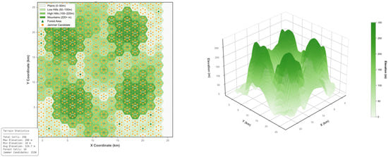
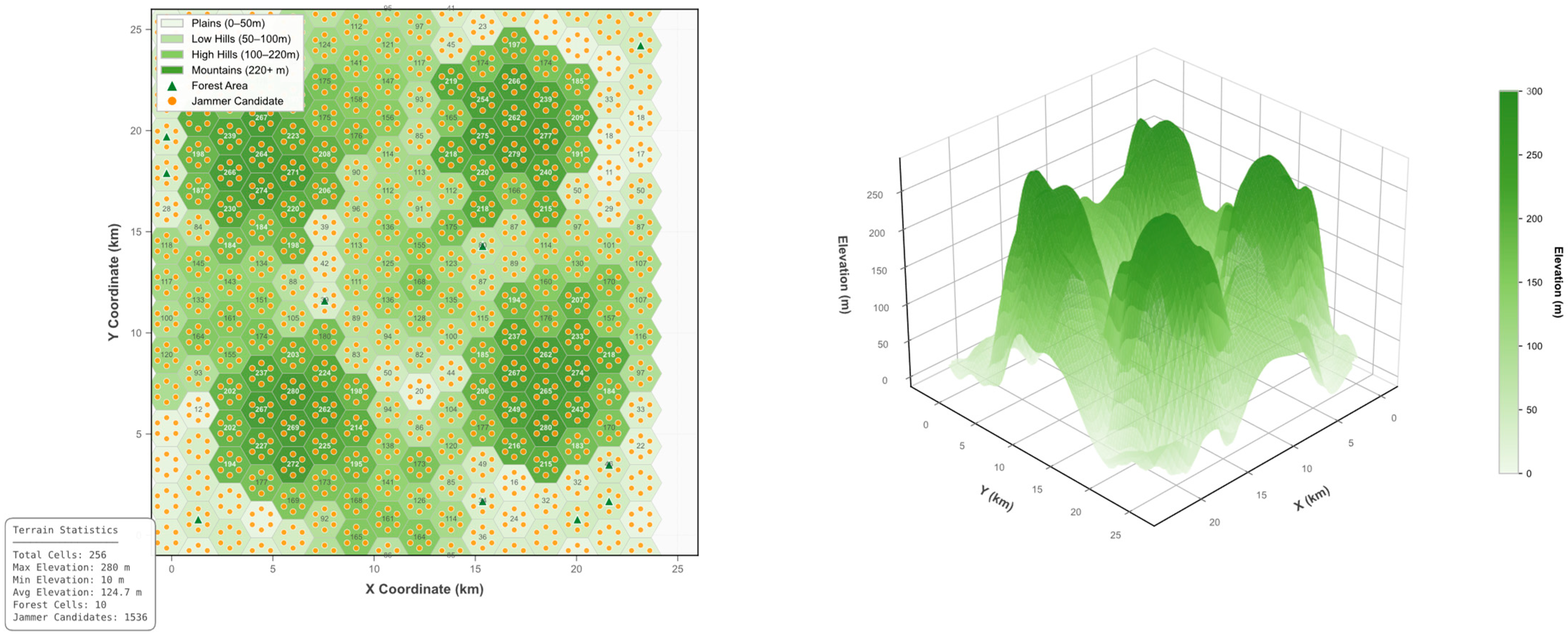
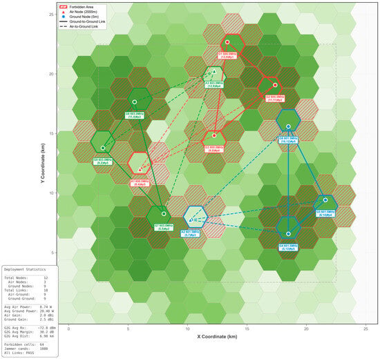
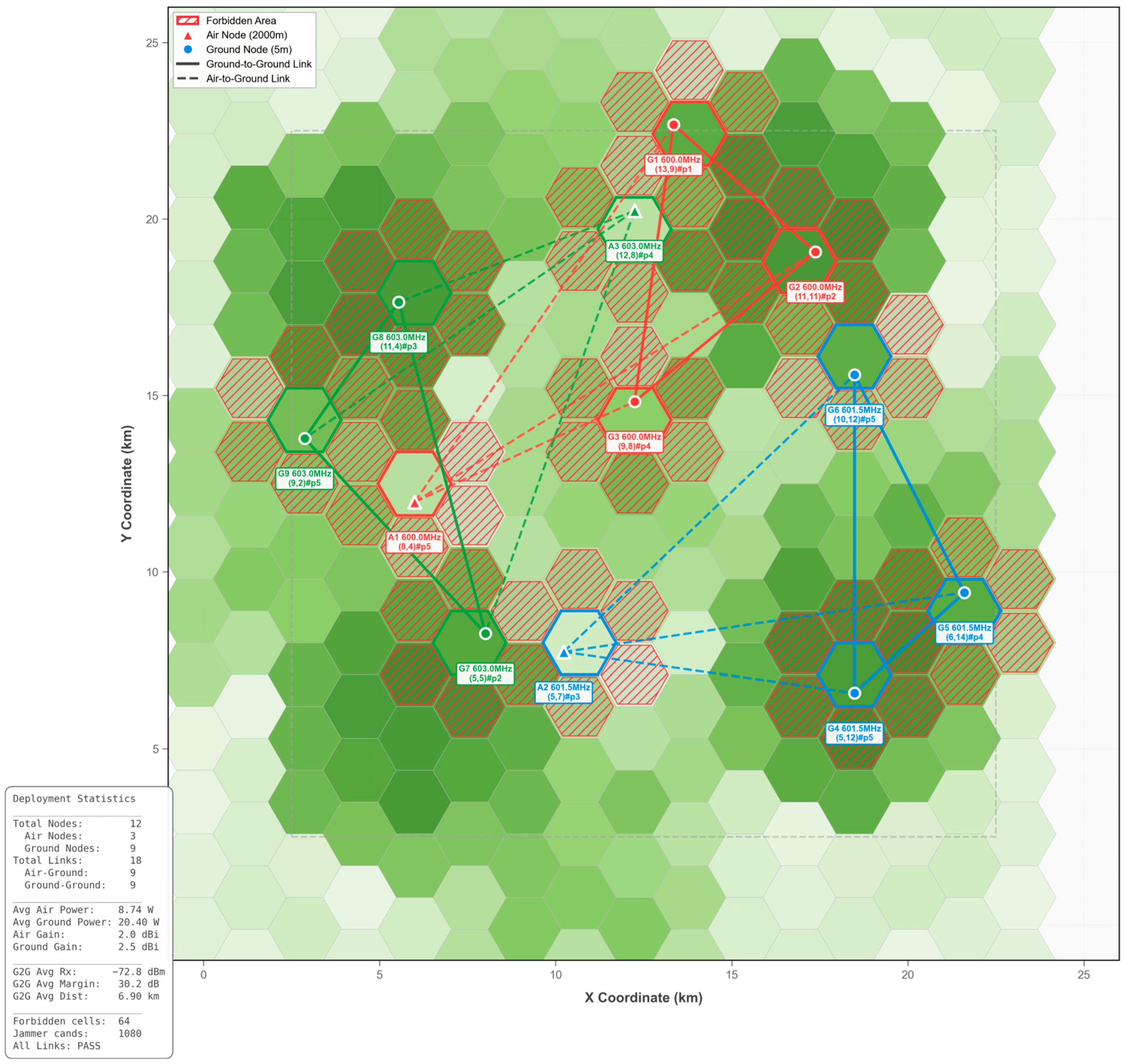
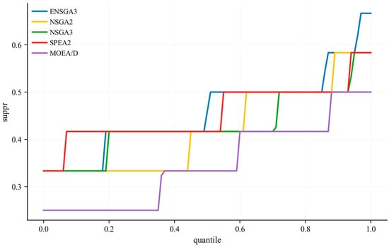
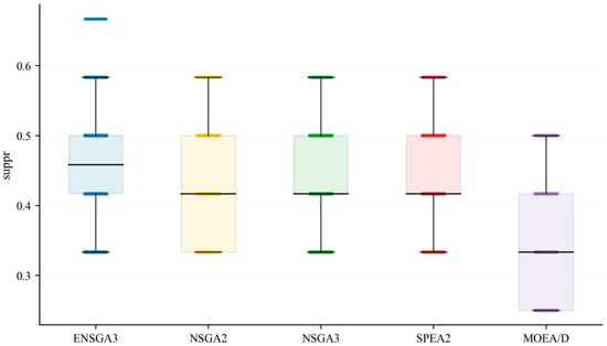
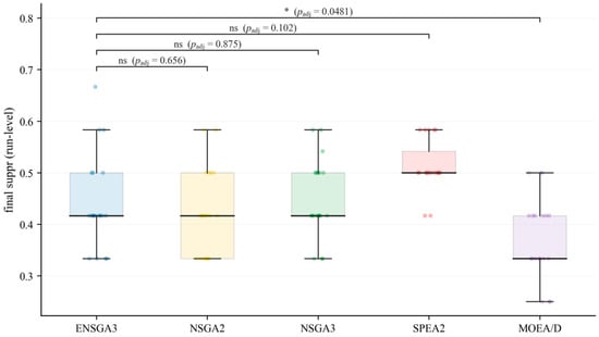
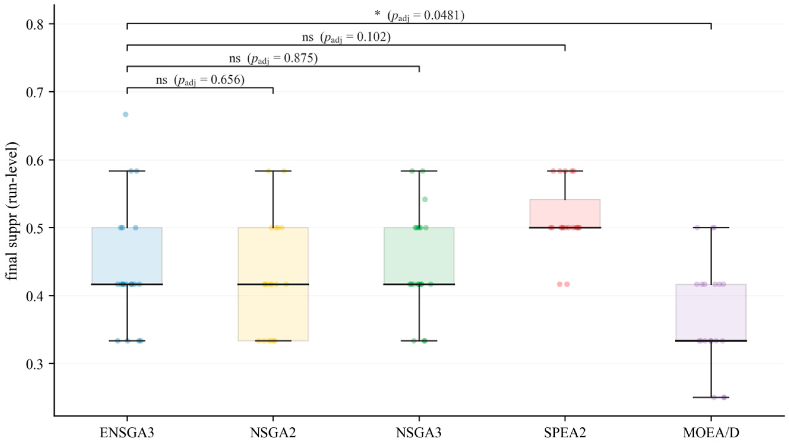
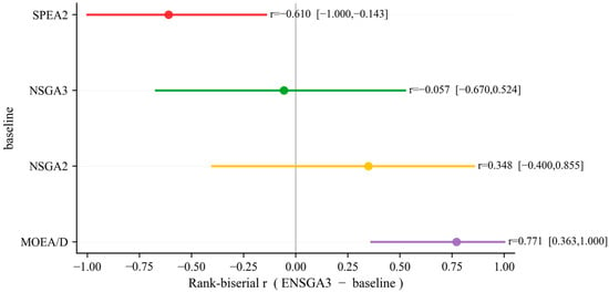
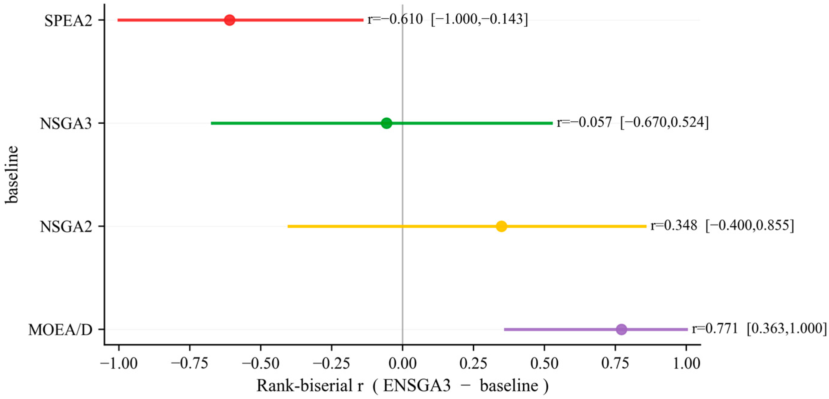
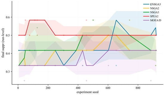
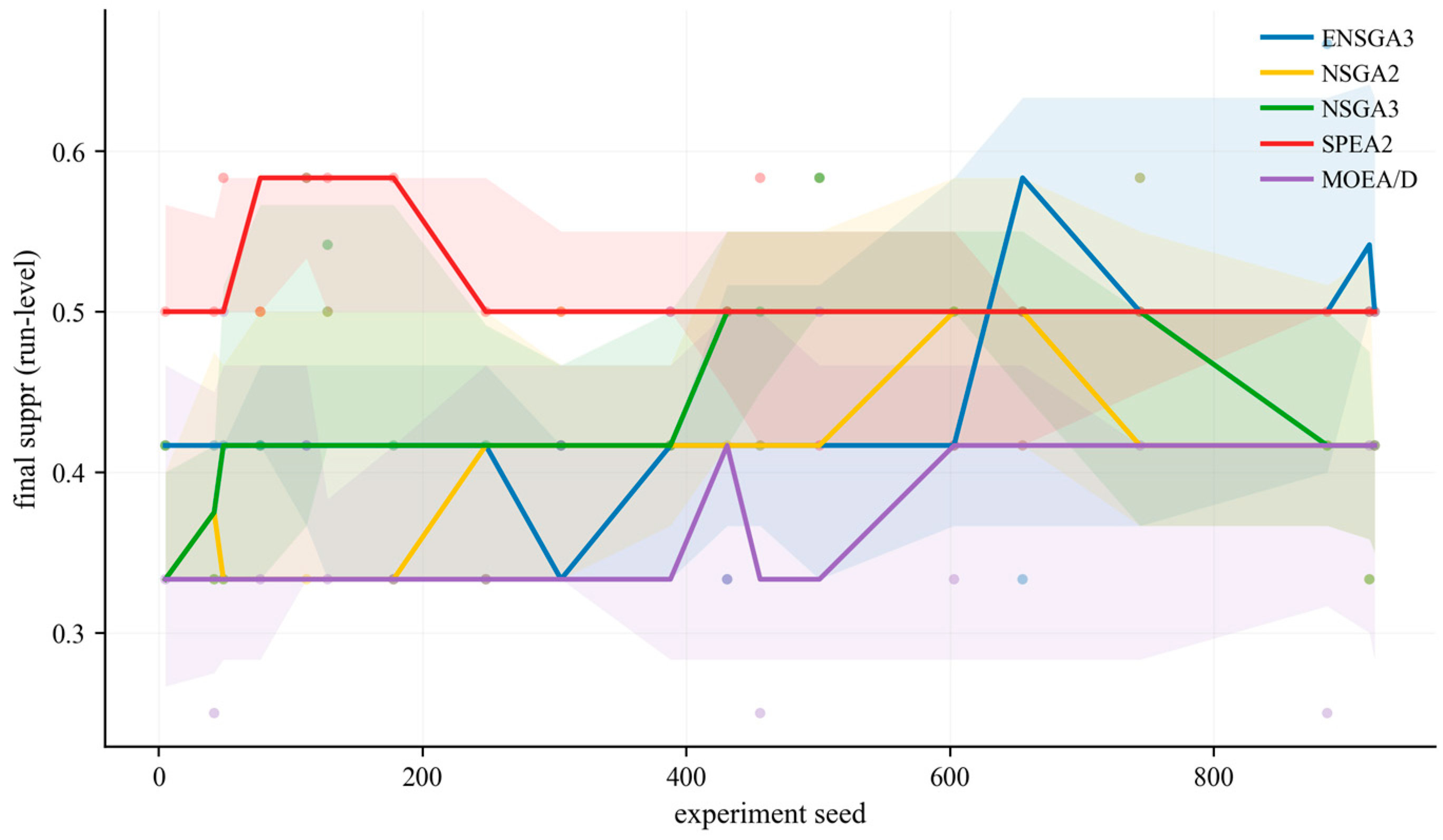
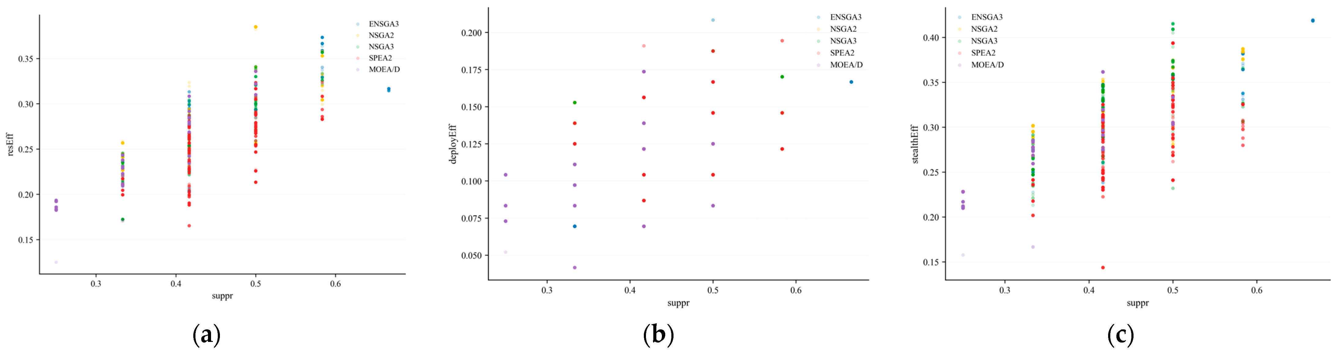
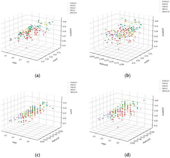
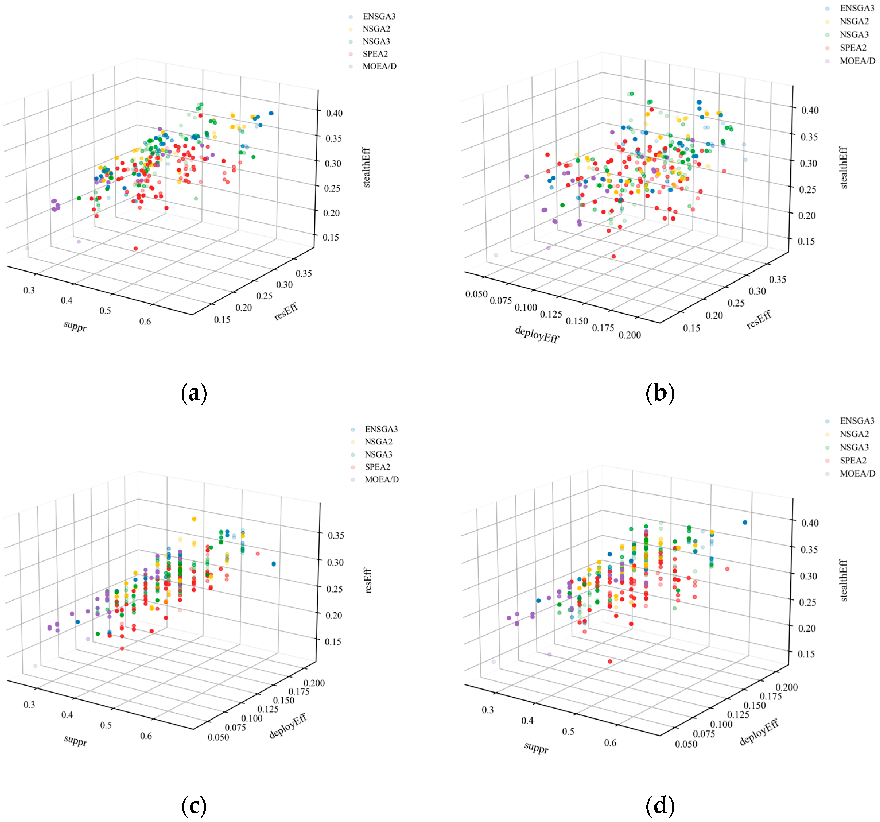
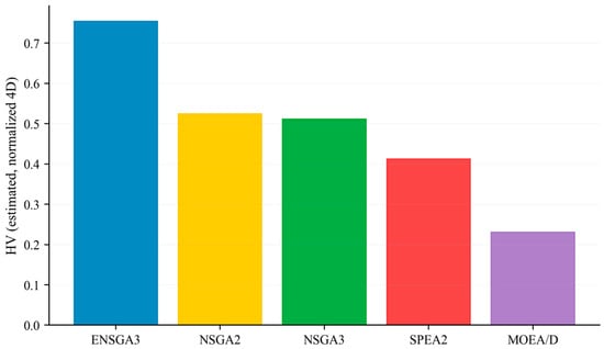
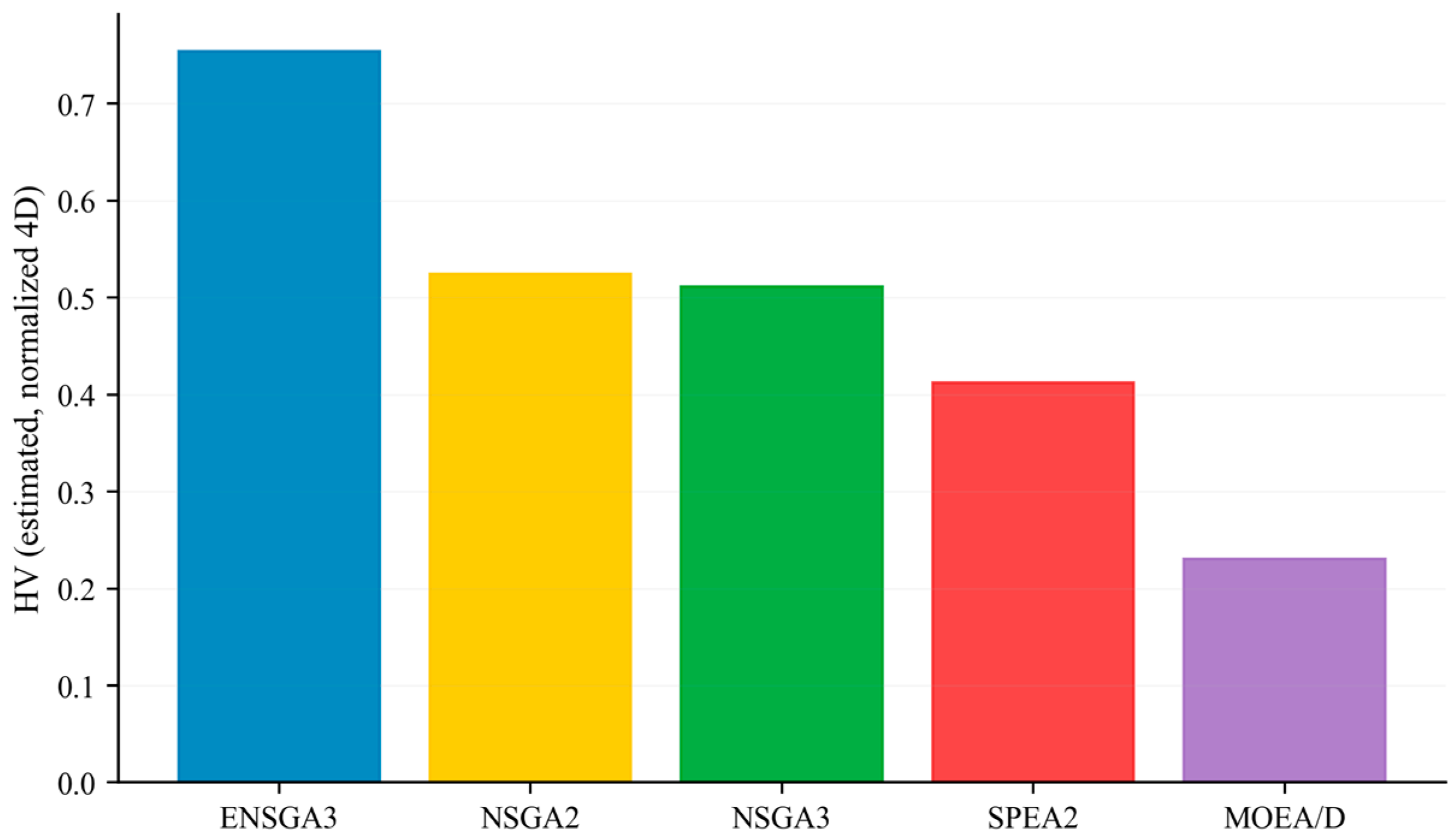
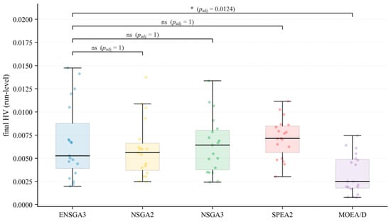
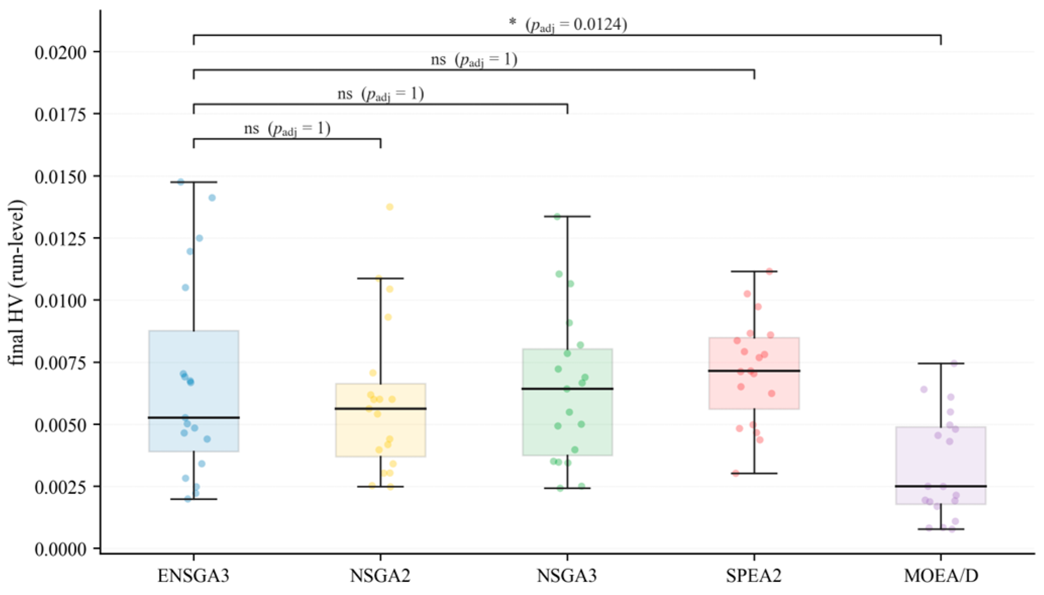
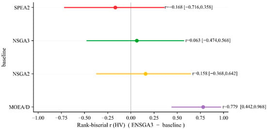
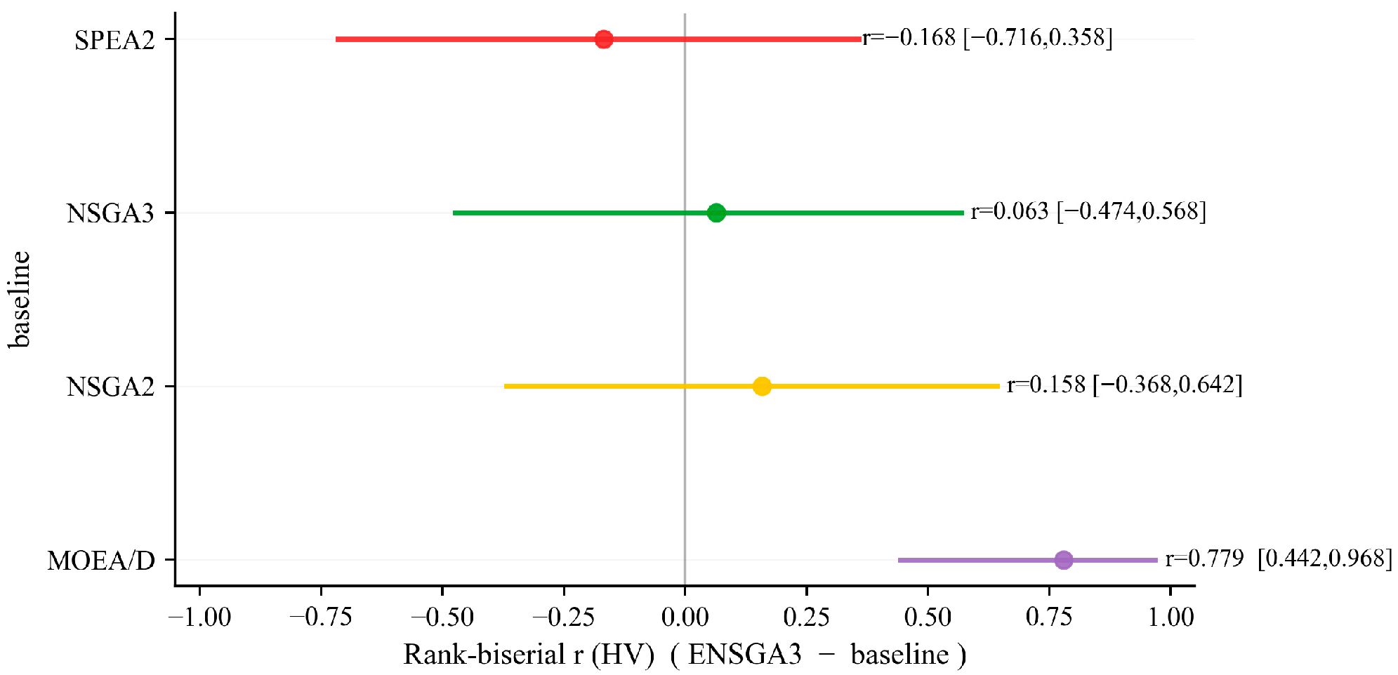
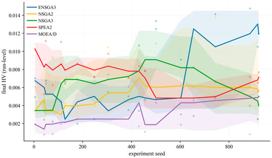
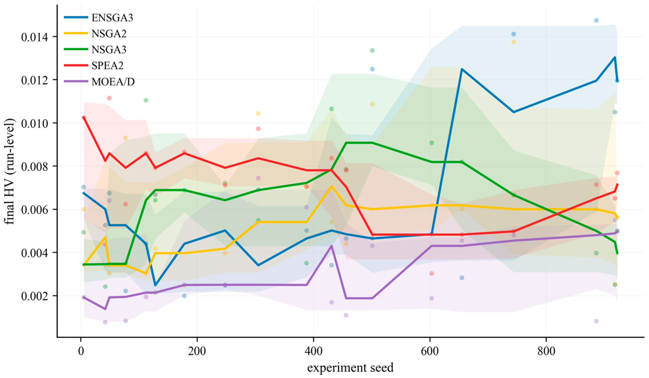
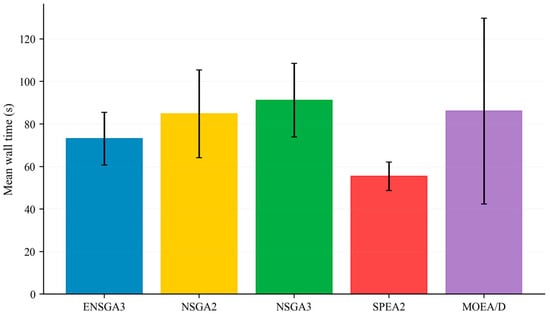
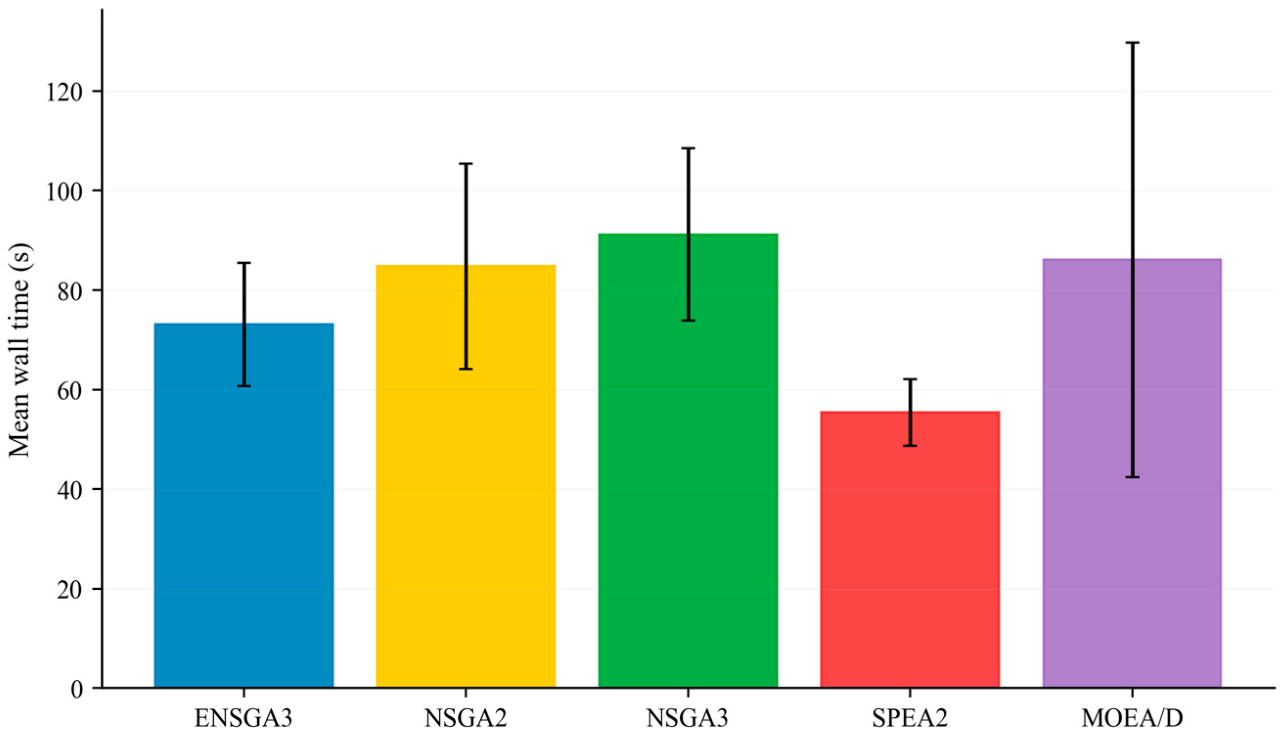
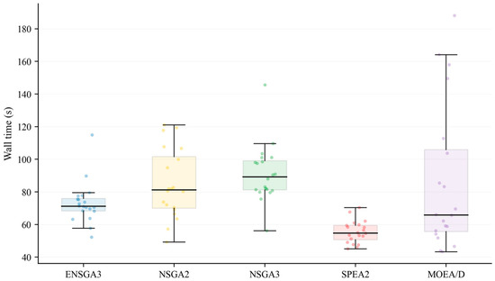
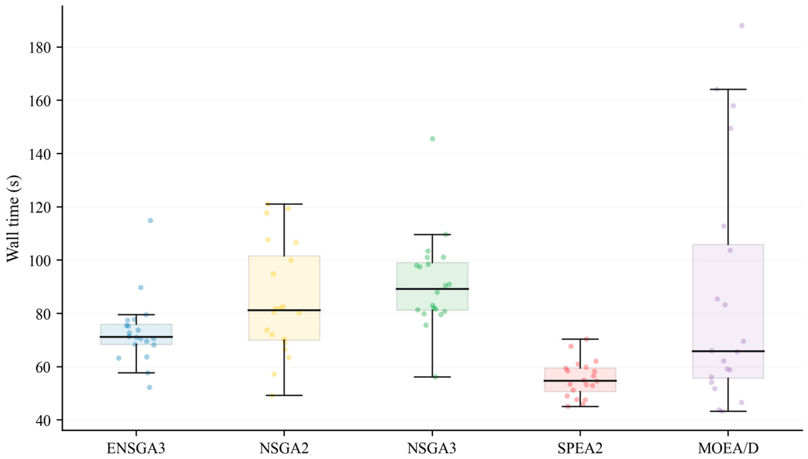
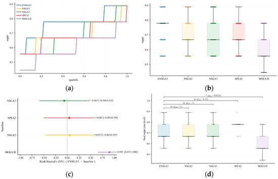
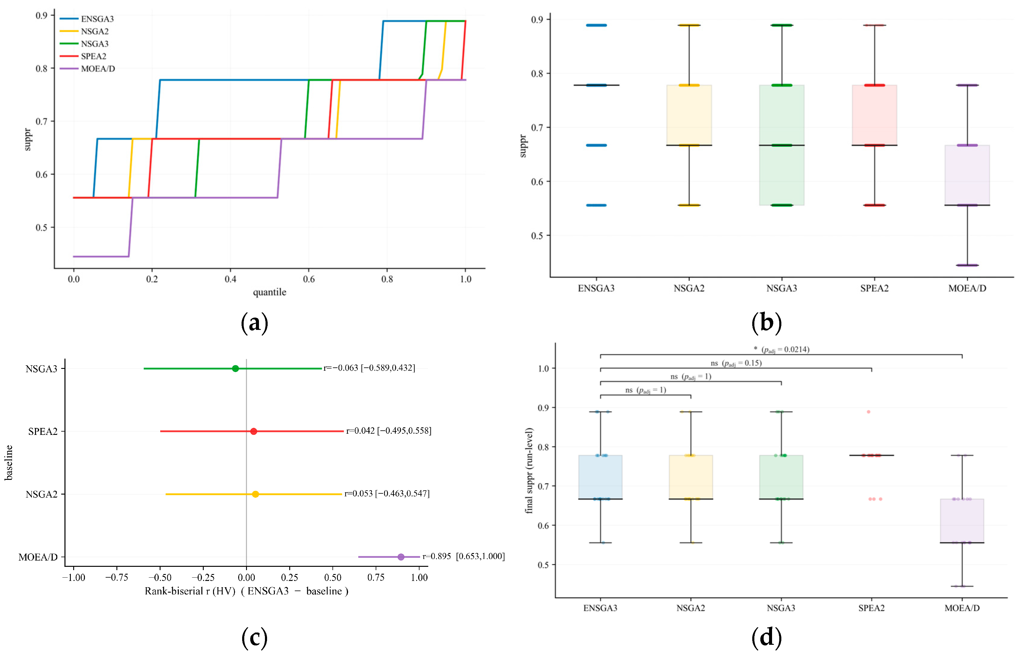
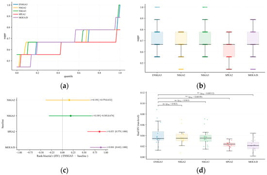
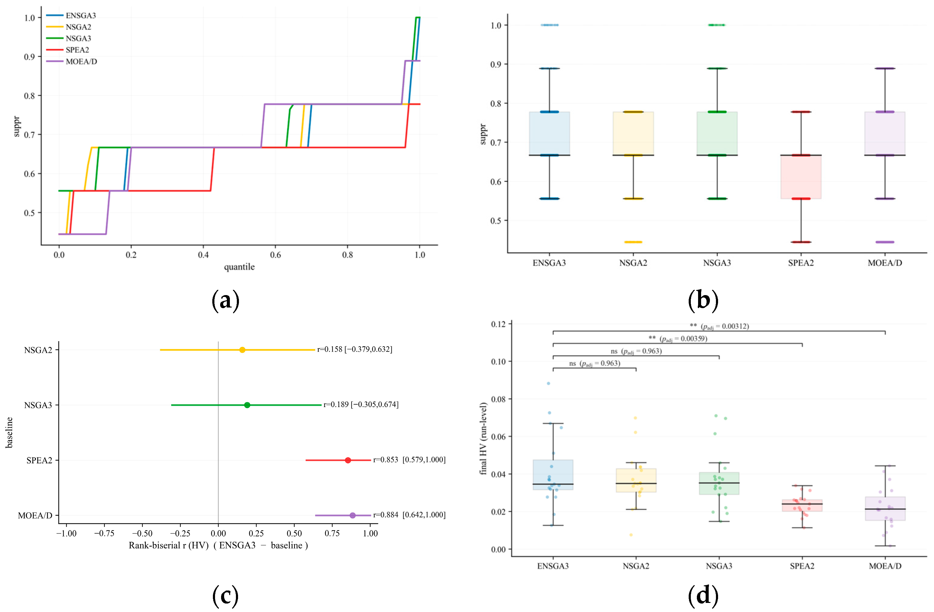
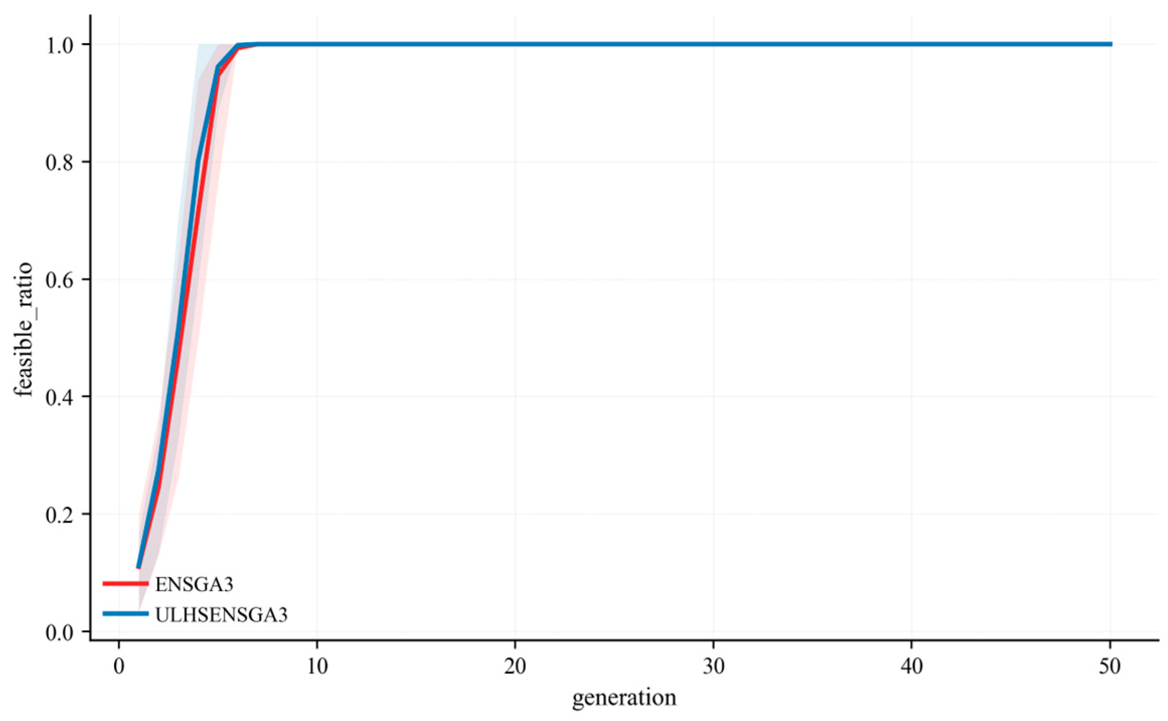
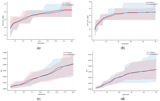
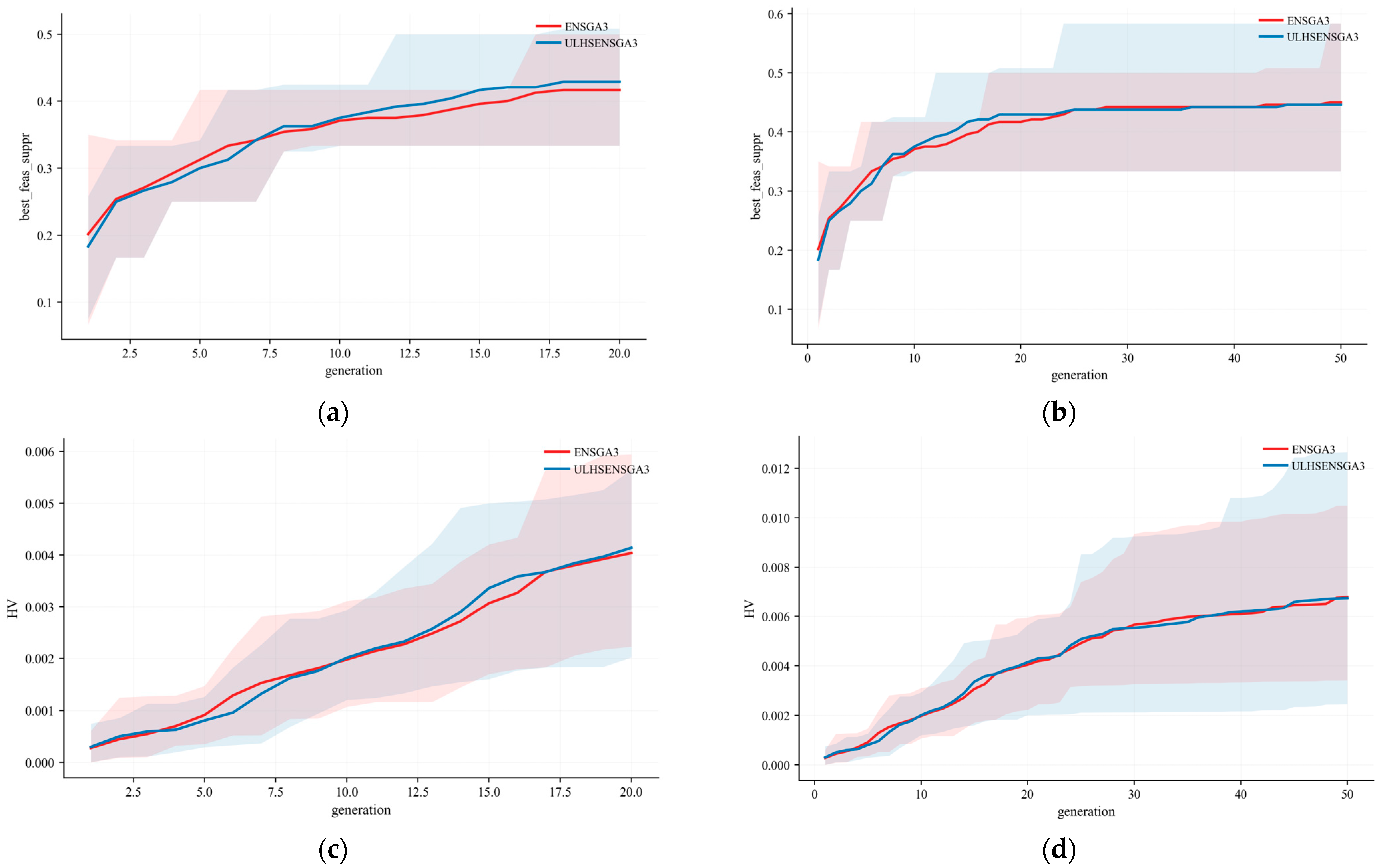
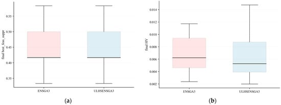
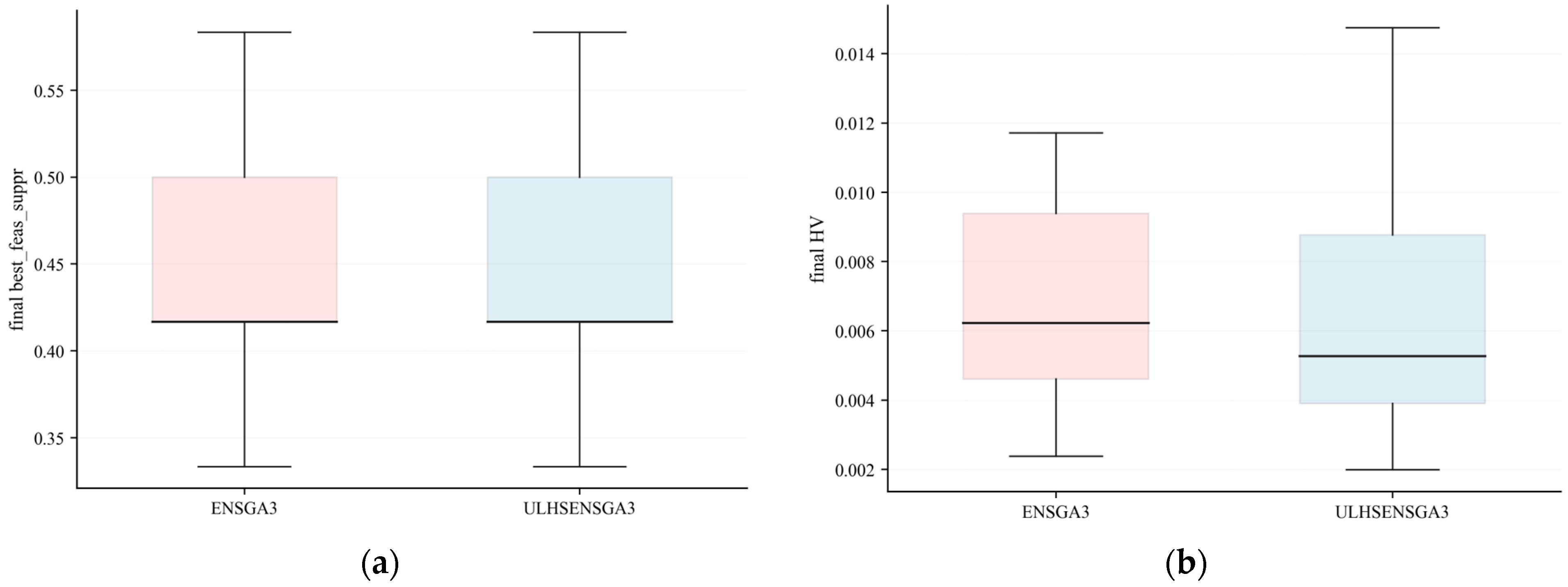
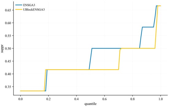
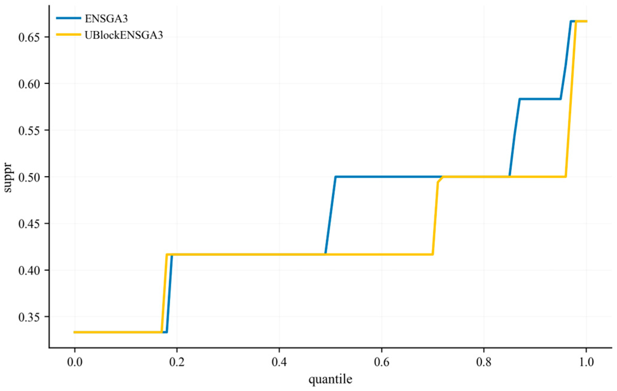
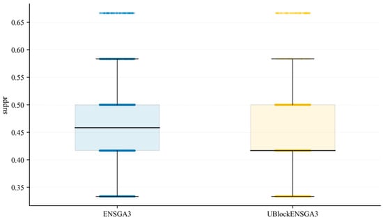
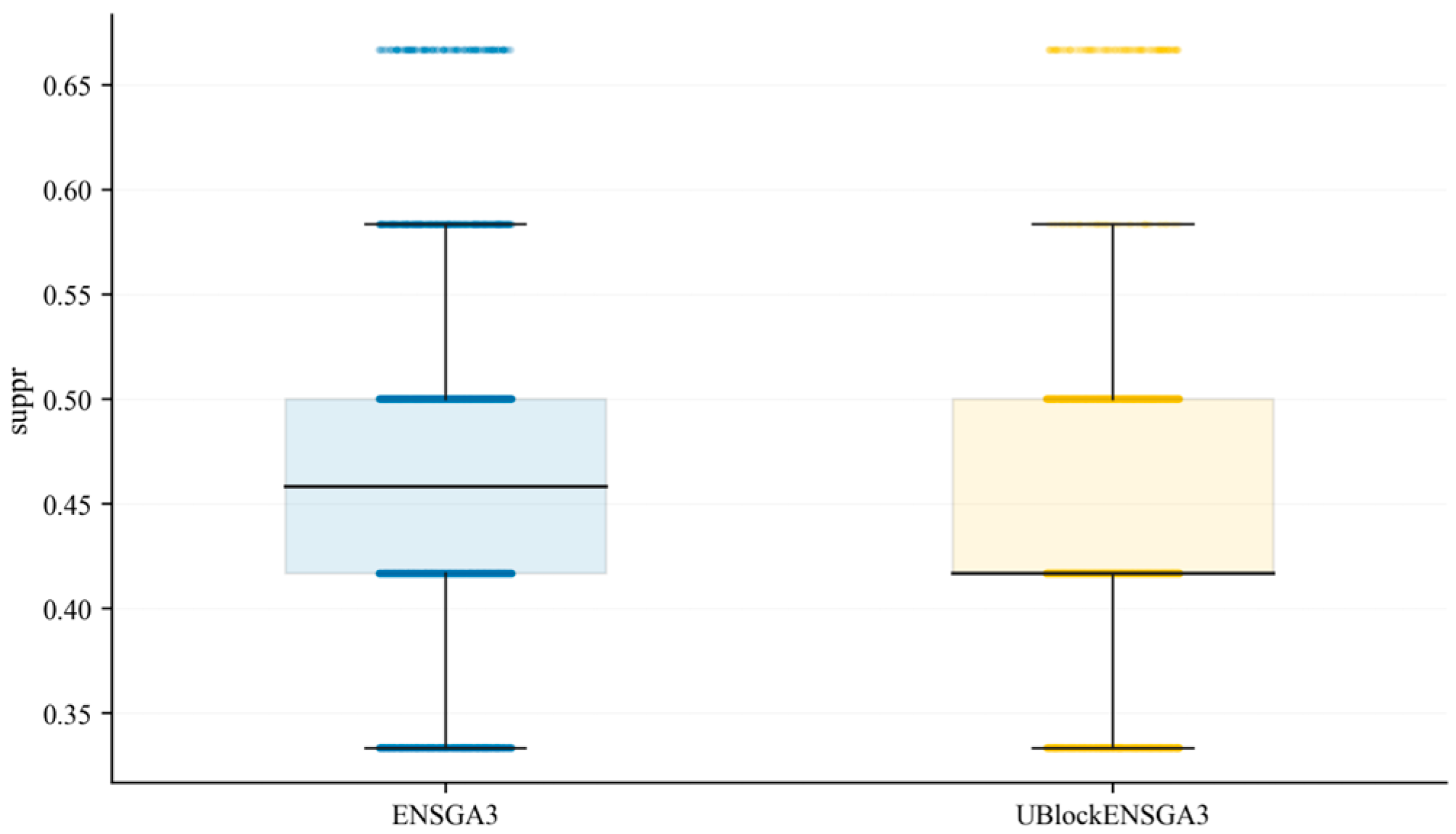
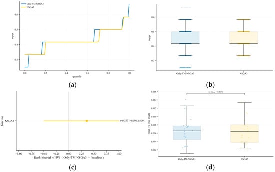
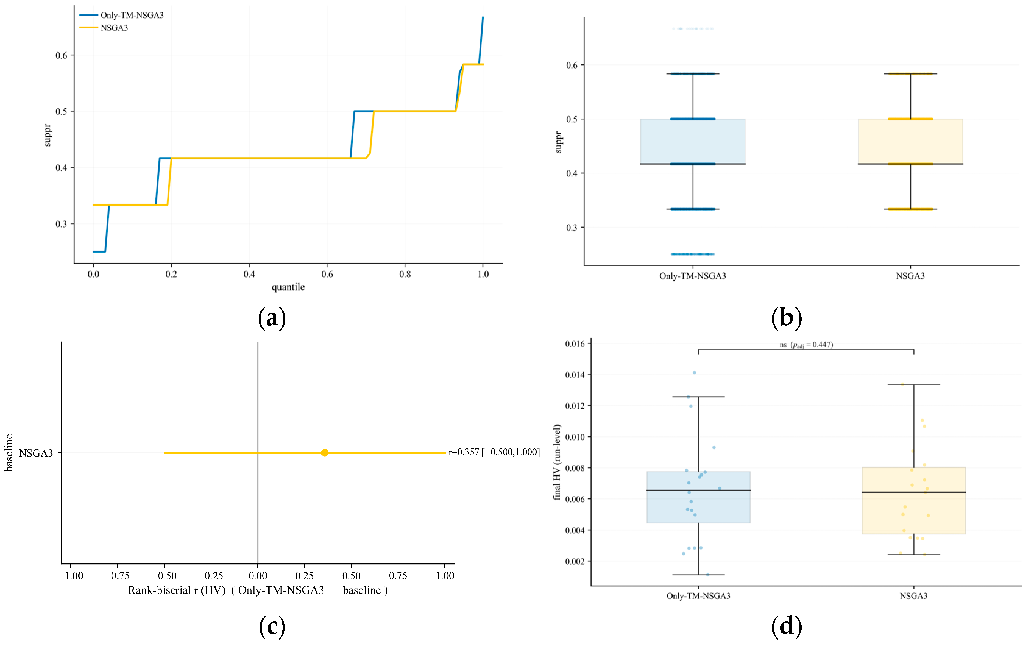

Disclaimer/Publisher’s Note: The statements, opinions and data contained in all publications are solely those of the individual author(s) and contributor(s) and not of MDPI and/or the editor(s). MDPI and/or the editor(s) disclaim responsibility for any injury to people or property resulting from any ideas, methods, instructions or products referred to in the content. |
© 2026 by the authors. Licensee MDPI, Basel, Switzerland. This article is an open access article distributed under the terms and conditions of the Creative Commons Attribution (CC BY) license.