


Abstract
Accurate delineation of cardiac structures in cardiac magnetic resonance (CMR) images is a prerequisite for quantifying cardiac function. This paper presents an end-to-end pipeline for automated cardiac segmentation and five-class pathology classification, evaluated on the 150 patients of the Automated Cardiac Diagnosis Challenge (ACDC) dataset. Three U-Net-based networks were trained with a hybrid cross-entropy-Dice loss selected through an ablation study and combined through soft-voting and weighted ensembles. On the official test set, the weighted ensemble achieved a mean Dice score of 90.27% at the slice level and 86.23% in volumetric evaluation, matching the best individual network and significantly outperforming the other two. Biomarkers extracted from the ensemble masks agreed closely with ground-truth-derived values (left ventricular ejection fraction: intraclass correlation 0.975) and were used to train nine machine learning classifiers under nested cross-validation. The four best classifiers achieved macro F1 scores between 88.73 and 89.14%. A cross-source evaluation across five segmentation sources showed no significant difference between classification based on automatically derived biomarkers and on ground-truth-derived biomarkers. SHAP analysis identified class-specific biomarkers consistent with cardiac pathophysiology. The results demonstrate technical feasibility on a public benchmark; external multi-center validation is required before clinical use.
1. Introduction
Cardiovascular disease is the leading cause of mortality, causing nearly 18 million deaths every year globally. A detailed analysis of cardiac morphology and function is required for early detection of cardiac disorders and for improvement of patient outcomes [1,2]. In recent decades, cardiac magnetic resonance (CMR) has become the gold standard in the assessment of cardiac morphology and function, providing excellent soft tissue contrast and enabling precise measurement of ventricular volumes, ejection fractions, and myocardial mass [3]. Despite its diagnostic value, the clinical utility of CMR is limited by the complex, labor-intensive and time-consuming process of manual image analysis, as well as its susceptibility to errors and inter- and intra-observer variability in structure delineation, which hinders the scalability of CMR analysis in clinical workflows [1,4].
Accurate segmentation of cardiac structures—left ventricle (LV), right ventricle (RV), and myocardium (MYO)—is a prerequisite for the extraction of clinical biomarkers such as ejection fraction, end-diastolic and end-systolic volumes, or the myocardial wall thickness, all of which are fundamental parameters in the diagnosis of cardiac diseases such as heart failure, hypertrophic cardiomyopathy, and coronary artery disease [1,2,3]. Therefore, the development of automatic segmentation methods has become an important research topic in cardiovascular imaging, having benefited from exponential progress in artificial intelligence (AI), especially convolutional neural networks (CNNs), which have achieved performance comparable to that of medical experts and have shown promise for enabling faster diagnosis and facilitating integration into clinical workflows [1,4,5].
Among these, the U-Net architecture has established itself as the most popular framework for biomedical image segmentation and is extensively used in cardiac MRI analysis. Its performance and robust architecture have motivated the development of numerous extensions. A systematic comparison of U-Net variants [6]—including Residual U-Net, Attention U-Net, Feature Pyramid U-Net, and Feedback Residual U-Net—demonstrates that residual connections make learning complex morphological patterns easier and benefit right ventricular segmentation, while attention mechanisms facilitate LV delineation. The right ventricle is an especially difficult structure to segment due to its irregular geometry and high inter-patient morphological variability [4]. The original U-Net does not particularly excel in any specific category but instead delivers consistently satisfactory results across all structures. While these studies demonstrate the relative strengths of individual architectures, to the best of our knowledge, the combination of these variants through ensemble strategies has rarely been evaluated at the level of the derived clinical biomarkers.
Beyond individual U-Net variants, the ACDC established a reference benchmark for both segmentation and diagnosis [7]. The best-performing segmentation method, which used an ensemble of 2D and 3D U-Nets, obtained Dice coefficients between 0.90 and 0.97 on the official test set, and most methods reproduced the clinical indices with LVEF correlations above 0.97 [7,8]. Self-configuring frameworks such as nnU-Net [9] and hybrid CNN-transformer architectures such as TransUNet [10] and Swin-Unet [11] have since been proposed, with mean Dice values of approximately 90% reported on subsets of the ACDC training data. For diagnosis, all four classification methods of the challenge relied on features derived from the segmentation masks and achieved test-set accuracies between 86% and 96% [7].
Loss function selection drastically affects segmentation performance, especially in the presence of class imbalance between foreground structures and background. Previous studies have reported advantages of using hybrid loss functions over individual loss functions [6,12]. In these studies, the loss function was selected based on quantitative segmentation metrics, and training convergence stability was not considered as an explicit selection criterion. However, convergence stability is especially important when using small datasets, where validation metrics are sensitive to individual patient cases.
Several works address the integration of automated segmentation with subsequent cardiac disease classification, forming complete computer-aided diagnosis (CAD) pipelines. Bhatia et al. [13] propose a system that includes a 3D GAN-based segmentation network as well as a random forest classifier trained on 28 clinically derived features, including ejection fractions, ventricular volumes, myocardial mass, body surface area, and volumetric ratios, achieving 99% accuracy on the ACDC dataset, and demonstrate that ratio- and difference-based features carry greater discriminative value than raw volumetric or anthropometric measurements. In [12], a multi-task architecture combining DenseNet and 3D U-Net simultaneously optimizes segmentation and classification through a shared encoder, lowering the diagnostic error rate from 32% to 22%, and speeding up convergence, compared to a classification-only model. However, neither study quantified the impact of segmentation quality on diagnostic performance. Additionally, interpretability analyses in existing CMR pipelines have rarely been extended to per-class feature attribution compared against established cardiac pathophysiology.
Based on the literature review above, the following research gaps were identified:
- To the best of our knowledge, comparative studies of U-Net variants have rarely combined the variants through ensemble strategies and assessed the effect of the combination on the derived clinical biomarkers;
- Limited evidence exists regarding the impact of segmentation quality on downstream diagnostic performance, when multiple segmentation sources and multiple classifiers are compared within the same evaluation framework;
- Few studies have examined whether overlap metrics, which are frequently used as the main or sole criterion for model selection, reflect the downstream diagnostic performance of segmentation outputs;
- In the studies reviewed, training convergence stability was not used as an explicit criterion for loss function selection in small dataset cardiac segmentation contexts;
- Per-class SHAP analysis, with the identified biomarkers compared against established cardiac pathophysiology, has rarely been applied to cardiac MRI pipelines operating on segmentation-derived biomarkers.
Beyond their diagnostic value, automated CMR pipelines can be incorporated within networked healthcare infrastructures instead of being used as standalone analysis tools. By integrating AI-based diagnostic pipelines with cloud-based Picture Archiving and Communication Systems (PACS) and telemedicine platforms, CMR images acquired at one site can be segmented, quantified, and classified remotely, which supports centralized diagnostic support for hospitals without on-site cardiac imaging expertise. The evolution of the Internet of Medical Things (IoMT) has allowed the delivery of scalable, low-latency diagnostic services by connecting distributed acquisition devices, cloud or edge computing resources, and remote decision-support systems through healthcare networks. A modular end-to-end pipeline such as the one proposed in the present study is well suited to such deployment. Each stage of the pipeline—segmentation, feature extraction, diagnostic classification, and interpretability—can be hosted as independent services and orchestrated over a network, rather than requiring monolithic on-premise software. In the present study, this networked deployment is discussed as the application context of the pipeline (Section 4.7); the IoMT, cloud, and network components were not implemented or evaluated. The experiments therefore concern the segmentation, biomarker extraction, classification, and interpretability stages.
In the present work, a modular end-to-end pipeline for cardiac structure segmentation and five-class cardiac pathology classification from CMR images is proposed and evaluated on the ACDC dataset. The individual components of the pipeline are established methods: U-Net, Residual U-Net, and Attention U-Net for segmentation, soft-voting and weighted ensemble, conventional supervised ML classifiers, and SHAP for interpretability. Accordingly, the contribution of the present work is methodological and integrative. It consists of: (i) the integration of these components into a single reproducible pipeline, from CMR images to segmentation-derived biomarkers, diagnostic classification, and feature attribution; (ii) a systematic cross-source evaluation, defined here as the comparison of downstream classification performance across segmentation sources (ground-truth annotations and four automated segmentation methods) within the same dataset, in which the same classification protocol is applied to the biomarkers derived from five segmentation sources and evaluated with four classifiers, in order to quantify how the segmentation source affects downstream diagnostic performance; (iii) a loss-function ablation study in which training convergence stability is used as an explicit selection criterion alongside segmentation metrics; and (iv) a per-class SHAP analysis comparing the dominant features of each diagnostic class with established cardiac pathophysiology. Therefore, the novelty of the present study lies in the integration of these established components and in their joint evaluation within a single protocol, which links segmentation quality, biomarker fidelity, and downstream diagnostic performance.
On the ACDC dataset, the biomarkers resulting from the proposed pipeline exhibit class-wise distributions which are consistent with established cardiac pathophysiology. The classification performance obtained with automatically derived biomarkers did not differ significantly from that obtained with ground-truth annotations. These results support the technical feasibility of the approach. Its clinical applicability remains to be established through the additional validation steps discussed in Section 4.6.
2. Materials and Methods
2.1. Overall Pipeline
The proposed pipeline comprises three sequential stages: cardiac structure segmentation from CMR images, biomarker extraction from the segmented masks, and multi-class pathology classification with an interpretability analysis. The complete methodology is presented in Figure 1.
Figure 1.
Overview of the proposed end-to-end pipeline. Stage 1 (cardiac segmentation): the 100 patients of the ACDC training set are partitioned at the patient level into training, validation, and internal test subsets, while the 50 patients of the ACDC test set are held out for evaluation; a loss function ablation study determines the loss function used for all subsequent experiments; three U-Net variants (U-Net, Attention U-Net, and Residual U-Net) are trained under identical configurations and combined through soft-voting and weighted ensembles. Stage 2 (biomarker extraction): clinical biomarkers are extracted from the segmentation masks of five sources (ground-truth annotations and four automated sources), and a physiological quality-control step defines the cohorts used for the main classification analysis (149 patients) and for the cross-source comparison (146 patients). Stage 3 (multi-class classification and interpretability): nine classifiers are evaluated in baseline and hyperparameter-optimized configurations using repeated stratified 5-fold cross-validation with five repetitions, followed by the cross-source evaluation and SHAP-based interpretability analysis. The classification stage is additionally evaluated on the 50 test patients after training on the ACDC training patients only (Section 2.9).
In the first stage, prior to the decomposition of the volumes into 2D slices, the patients of the ACDC dataset are partitioned at the patient level. The original ACDC partition was preserved: the 100 patients of the ACDC training set are divided, with a fixed random seed, into training (80 patients), validation (10 patients), and internal test (10 patients) subsets. The 50 patients of the ACDC test set are not used at any stage of training or model selection and are reserved for the evaluation of segmentation performance and for the hold-out classification evaluation. The validation subset is used for checkpoint selection, loss-function selection, and ensemble-weight selection. A systematic ablation study over candidate loss functions is implemented to identify the optimal loss function to be used in all subsequent segmentation experiments. Three U-Net-based networks (U-Net, Residual U-Net, and Attention U-Net) are trained under the same experimental configuration, and their predictions are combined through two ensemble strategies: soft voting and weighted ensemble. The ensemble weights are selected based on the mean Dice coefficient obtained on the validation subset.
In the second stage, segmentation masks are generated for all 150 patients by each of the three individual networks and by the weighted ensemble. Together with the ground-truth annotations, they form five segmentation sources. For the 80 patients used to train the networks, the automatically generated masks are in-sample predictions, whereas the masks of the 50 test patients are produced by networks that did not see them during training or model selection; this aspect is addressed in Section 3.3 and Section 4.6. From the masks of each of the segmentation sources, a structured set of clinical biomarkers is extracted. A physiological quality-control step is then applied to the extracted biomarkers, which defines the cohort of 149 patients used for the main classification analysis and the common cohort of 146 patients used for the cross-source comparison (Section 2.8).
In the third stage, the biomarkers extracted from the weighted-ensemble masks are used as input to a multi-class classification pipeline that evaluates nine supervised ML models in baseline and hyperparameter-optimized configurations. Model performance is estimated by repeated stratified 5-fold cross-validation with five repetitions, and hyperparameter optimization is performed within the training portion of each outer fold. To assess the effect of the segmentation source on downstream diagnostic performance, a cross-source evaluation is then performed by applying the same classification protocol to the biomarkers extracted from each of the five segmentation sources. Finally, SHAP analysis is applied to the best-performing tree-based classifier to quantify the contribution of individual biomarkers to each diagnostic class.
2.2. The ACDC Dataset
The Automated Cardiac Diagnosis Challenge (ACDC) dataset was originally introduced at the MICCAI 2017 conference, containing clinical examinations acquired from real-world patients in the University Hospital of Dijon, France. The ACDC dataset is among the most widely used datasets for cardiac structure segmentation and is designed for the evaluation of automatic algorithms for the analysis of the ventricles and myocardium in different cardiovascular pathologies [7].
The dataset comprises 150 clinical examinations, with 100 allocated to the training set and the remaining 50 to the testing set. For each patient, the dataset provides short-axis cine-MRI images, acquired over the course of a complete cardiac cycle. The ground-truth (GT) masks, i.e., the expert annotations provided with the dataset, are only available for the two standard moments of the cardiac cycle: end-diastole (ED) and end-systole (ES). The ground-truth annotations include the three cardiac structures: left ventricle, right ventricle, and myocardium, as well as the background. Images are stored in NIfTI format with their native voxel spacing; all volumetric measurements are computed in the native image geometry using the voxel spacing from the NIfTI header.
The dataset also classifies patients into 5 categories, providing labels corresponding to different cardiovascular pathologies. The 150 patients are evenly distributed across the five classes, with 30 patients in each class:
- NOR—healthy subjects with no cardiac afflictions;
- DCM—dilated cardiomyopathy;
- HCM—hypertrophic cardiomyopathy;
- MINF—previous myocardial infarction;
- RV—abnormal right ventricle.
The 3D volumes of the ACDC dataset were decomposed into individual short-axis slices to enable their use for 2D model training. The partition into subsets was performed at the patient level before this decomposition, so that all slices of a patient belong to the same subset to avoid data leakage. The ED and ES volumes of the 100 training patients yield 1902 2D slices, and those of the 50 test patients yield 1076; the number of slices per patient depends on the number of slices per volume. A representative example from the dataset is provided in Appendix A (Figure A1), while the ground-truth segmentations at ED and ES for each pathology class are illustrated in Figure 2.
Figure 2.
Examples of CMR slices and the corresponding segmentations for the five pathologies in the dataset, shown at the ED and ES phases, in the following order: DCM, HCM, MINF, NOR, and RV.
Table 1 summarizes the number of patients and slices in each subset and their use in the pipeline.
Table 1.
Patient-level partition of the ACDC dataset and use of each subset in the pipeline. Slice counts apply only to the segmentation stage; n.a.: not applicable.
2.3. Segmentation Architectures
The U-Net architecture was first introduced by Ronneberger et al. in [14] for biomedical image segmentation. It follows a symmetrical encoder–decoder structure and has since become one of the most widely used architectures for medical imaging analysis tasks.
The encoder uses repeated blocks of two 3 × 3 convolutions with Rectified Linear Unit (ReLU) activations, followed by a 2 × 2 max-pooling with a stride of 2, to progressively extract hierarchical feature representations. Each encoder level halves the spatial resolution and doubles the number of feature channels. The decoder then reconstructs the spatial resolution through successive 2 × 2 transposed convolutions. These are followed by concatenation with the corresponding encoder feature maps using skip connections.
Skip connections link the encoder and decoder at each resolution level. They are a defining element of the U-Net architecture, preserving fine-grained spatial information, while allowing the network to generate segmentation masks with precise boundary delineation. The bottleneck block is another important characteristic element of the architecture. It consists of two 3 × 3 convolutions, and it is responsible for capturing highly abstract feature representations before decoding.
Residual U-Net is an extension of the U-Net architecture which improves the original network by increasing the stability of the optimization process and improving gradient flow [15]. By replacing the convolutional blocks with residual blocks, the network is allowed to learn residual mappings. Each residual block introduces a shortcut connection that adds the input to the output of the convolutional path. The following equation can be used to define the output of a residual block:
where x is the block input and F(x;W) represents the transformation applied by the convolutional layers with learned parameters W. This identity shortcut facilitates gradient flow during backpropagation, mitigates the vanishing gradient problem, and enables deeper network training without loss of performance. The residual formulation provides the network with a mechanism to learn incremental refinements to the input representation, rather than complete mappings, leading to improved optimization stability.
y = x + F(x; W),
In 2018, the Attention U-Net architecture was designed to make the network more sensitive to relevant areas of the image, minimizing the effect of the background and of other irrelevant structures [16]. This U-Net extension is particularly useful for structures where the morphology varies greatly, the boundaries are not well-defined, and where the contrast between the structure and surrounding tissue is low, as is often the case in medical imaging.
Attention U-Net enhances the standard U-Net architecture by integrating soft attention gates at each skip connection before the concatenation of encoder and decoder feature maps. In the conventional U-Net, all the feature maps produced by the encoder are transferred to the decoder. In the Attention U-Net architecture, attention gates suppress activations corresponding to the regions of the image which are irrelevant for the task, while responses in task-relevant regions are enhanced.
Each attention gate receives as input a gating signal g, containing high-level contextual information from the deeper decoder level, and a feature vector x from the corresponding encoder level, containing detailed spatial information. The two inputs are projected to a common dimensionality through 1 × 1 convolutions, after which they are summed and passed through a ReLU activation function, and then again projected and activated with a sigmoid activation function. This results in an attention coefficient map with values ranging from 0 to 1.
This map is then used to reweight the encoder feature maps before concatenation with the decoder. Attention U-Net uses soft attention, which, as opposed to hard attention, preserves end-to-end differentiability, and allows the attention mechanism to be trained jointly with the rest of the network via backpropagation.
All three architectures share the same channel progression, with 64, 128, 256, and 512 channels in the four encoder levels, 1024 channels in the bottleneck, and 512, 256, 128, and 64 channels in the corresponding decoder levels. Each convolutional block of U-Net and Attention U-Net consists of two 3 × 3 convolutions, each followed by batch normalization and a ReLU activation, and dropout with p = 0.1. Each block of Residual U-Net contains two 3 × 3 convolutions with batch normalization and ReLU activations, a residual shortcut connection, and spatial dropout (p = 0.1). The attention gates of Attention U-Net use intermediate channel dimensions of 256, 128, 64, and 32 at the 512-, 256-, 128-, and 64-channel levels, respectively. All networks were trained on single-channel 192 × 192 inputs and produce a four-class output (background, RV, MYO, and LV); being fully convolutional, they can also be applied to inputs of other sizes divisible by 16 (Section 2.4).
2.4. Experimental Configuration
To ensure a fair comparison between architectures, the same training configuration was used for all segmentation networks. Only the network architecture was varied, and, in the ablation study described in Section 2.6, the loss function. The configuration is summarized in Table 2.
Table 2.
Experimental configuration of the segmentation networks.
During training and slice-level evaluation, each 2D slice was resized to 192 × 192 pixels and normalized by per-slice z-score normalization:
where μI and σI are the mean and standard deviation of the slice intensities.
To avoid overfitting, online data augmentation using the Albumentations library was applied exclusively to the training set [17]. Augmentations included random rotations (±15°, p = 0.5), horizontal flipping (p = 0.5), affine transformations with scale variation (0.9–1.1) and shearing (±5°, p = 0.5), and elastic deformations (Albumentations parameters α = 20, σ = 4, p = 0.2).
All networks were trained with the hybrid CE-Dice loss defined in Equation (3), with α = 0.6 (a weight of 0.6 for the cross-entropy term and 0.4 for the Dice term), the configuration selected in the loss-function ablation study (Section 2.6 and Section 3.1):
where and are the values of the cross-entropy loss and the Dice loss, respectively, and α ϵ [0, 1] is a parameter that controls the relative contribution of each term.
Hybrid losses of this type combine the overlap sensitivity of the Dice loss with the pixel-level gradient stability of the cross-entropy loss [6,12]. The two terms can be defined as:
where pi,c is the softmax probability of class c at pixel i, gi,c is the one-hot reference label, N is the number of pixels in the mini-batch, C = 4, and ε = 10−8. The sums run over all pixels of the mini-batch, the cross-entropy term is unweighted, and the background class (c = 0) is excluded from the Dice term. The Dice term is normalized by C, as in the implementation used for all experiments. Relative to an average over the three foreground structures, this normalization scales the Dice term by the constant factor , and the values of α reported in the present study refer to the loss as defined in Equations (3)–(5).
The networks were trained for 50 epochs with a batch size of 16. The Adam optimizer was selected for its adaptive learning-rate properties and fast convergence on segmentation networks [18] and was used with an initial learning rate of 5 × 10⁻⁵ and a weight decay of 10−5. A ReduceLROnPlateau scheduler halved the learning rate when the validation loss did not decrease for five consecutive epochs. No early-stopping criterion was applied: all networks were trained for the full 50 epochs, and the checkpoint with the lowest validation loss was retained for evaluation. Model parameters were initialized using the default PyTorch initialization schemes, without additional custom initialization. For reproducibility, the random number generators were initialized with seed 42.
For the generation of the full segmentation masks used for biomarker extraction (Section 2.7), the trained networks were applied to each slice at its native in-plane resolution, after z-score normalization of the volume and zero-padding to a multiple of 16 pixels, and the predictions were cropped back to the original slice size. In this way, the masks share the native geometry of the images, and no interpolation of the label maps is required before volumetric analysis.
The pipeline was implemented in Python 3.12.0 using PyTorch 2.5.1 with CUDA 12.1 for the segmentation networks, and scikit-learn 1.7.2, XGBoost 3.2.0, CatBoost 1.2.10, and SHAP 0.50.0 for the classification and interpretability stages. NIfTI volumes were processed with NiBabel 5.3.2, and data augmentation was implemented with Albumentations 2.0.8. All experiments were performed on a single NVIDIA GeForce RTX 4060 Laptop GPU.
2.5. Ensemble Strategies
Two ensemble strategies were used to exploit the complementary strengths of the three individual architectures previously presented (U-Net, Residual U-Net, and Attention U-Net). This approach was based on the principle that combining diverse models reduces the error of the individual models, which has proven effective in recent DL segmentation pipelines for cardiac imaging, where ensembles of different U-Net variants have outperformed individual models [19].
The soft-voting ensemble computes the arithmetic mean of the probability maps for each pixel and then selects the class with the maximum mean probability. Mathematically, this can be expressed as:
where is the probability for class c predicted by model m. All models contribute equally to the final prediction.
In the weighted ensemble, the contribution of each model to the final prediction is scaled by a scalar weight, as follows:
The ensemble weights were selected by grid search on the validation subset. The weights of Attention U-Net (ωA) and U-Net (ωU) were varied over the set {0.20, 0.25, …, 0.85}, and the weight of Residual U-Net was obtained as:
ωR = 1 − ωA − ωU
Combinations that resulted in a value outside the interval [0, 1] for ωR were discarded. Each admissible combination was evaluated using the mean Dice coefficient over the three foreground structures (RV, MYO, and LV) on the validation subset, and the combination with the highest value was selected. The selected configuration (ωR = 0.4, ωA = 0.3, ωU = 0.3; Section 3.2) was used in all subsequent analyses. Both ensembles combine the probability maps generated at inference time, have no additional trainable parameters, and were evaluated in this form at the slice level (Section 3.2). For the full-volume masks used for biomarker extraction, the weighted ensemble was applied to the label maps of the three networks with the same weights (weighted majority voting), in which each voxel v is assigned the label:
where is the label predicted by model m, ωm is its weight, and 1[∙] is the indicator function. With the selected weights, each voxel receives the label on which at least two networks agree, and the Residual U-Net label when the three predictions differ.
2.6. Loss Function Ablation Study
One of the most important design choices in a cardiac structure segmentation task is the choice of the loss function, since a significant spatial imbalance between foreground and background and between the sizes of the structures can greatly bias the optimization process. Therefore, to select the most suitable loss function for the ACDC dataset, a systematic ablation study was performed, where the effect of the loss function is isolated by using the standard U-Net architecture with a fixed experimental configuration.
The following loss functions were tested:
- Dice loss, which optimizes the overlap between the predicted masks and the ground-truth masks, is robust to class imbalance, but can lead to unstable gradients on small structures;
- Cross-entropy loss, which operates at the pixel level and gives a more stable estimate of the gradient; cross-entropy is, however, sensitive to class imbalance;
- Hybrid loss: a weighted linear combination of the above two, defined as in Equation (3). For the hybrid loss, α values of {0.3, 0.4, 0.5, 0.6, 0.7} were evaluated.
To prevent the comparison between architectures from being affected by architecture-specific tuning, the loss configuration was selected on the standard U-Net and applied unchanged to Residual U-Net and Attention U-Net.
The optimal loss function was selected not solely based on quantitative segmentation metrics, but also on training stability, which was assessed by inspecting the loss and Dice curves across epochs and quantified by the standard deviation of the validation mean DSC over the last five epochs and by the root-mean-square epoch-to-epoch change in the validation mean DSC after epoch 10. Configurations that exhibited larger inter-epoch fluctuations, which are expected with small patient-wise validation subsets, were considered less stable and therefore less favorable in the selection process, even when their peak metric values were marginally higher. Robust and reproducible convergence behavior was prioritized over marginal performance gains.
2.7. Clinical Feature Extraction
Extraction of clinical biomarkers from segmentation masks allows the quantitative assessment of cardiac function and provides clinically relevant descriptors for downstream diagnostic tasks. Therefore, an automated procedure was developed for the extraction of clinical biomarkers from the 3D CMR NIfTI volumes at the ED and ES timepoints. The procedure was applied identically to the masks of five segmentation sources: the ground-truth annotations, U-Net, Residual U-Net, Attention U-Net, and the weighted ensemble. The segmentation labels follow the ACDC convention: 1 for the RV cavity, 2 for the MYO, and 3 for the LV cavity.
The segmentation networks were trained using the ACDC ground-truth reference annotations, which follow the convention of including papillary muscles in the LV cavity [7]. The automatically generated masks therefore follow this same labeling convention. Consequently, papillary muscles contribute to the LV cavity volume and are excluded from the myocardial volume and the LV mass. The treatment of trabeculations is not explicitly specified in the ACDC contouring protocol, so the automatically generated masks reproduce the convention implicitly adopted in the ground-truth annotations. According to the SCMR recommendations, papillary muscles and trabecular tissue are myocardial tissue and should ideally be included in the LV mass. In clinical practice, however, they are frequently included in the blood pool. Both approaches are considered acceptable provided they are applied consistently [20]. The convention adopted in the present study may therefore lead to slightly higher cavity volumes and slightly lower myocardial mass than protocols that assign these structures to the myocardium.
For each patient, the voxel dimensions were retrieved from the NIfTI file header, and the volume of a given anatomical structure was computed by counting all voxels assigned to the corresponding label:
where M(x, y, z) is the segmentation mask, l is the structure label, 1[∙] is the indicator function, ∆x, ∆y, ∆z are the voxel spacings in millimeters, and vvoxel is the voxel volume in milliliters. The through-plane spacing Δz corresponds to the slice spacing encoded in the NIfTI header and represents the distance between consecutive slices, thereby accounting for the slice thickness and interslice separation in the volumetric calculation.
A set of cardiac functional biomarkers was derived from the extracted volumes as follows:
where ρMYO = 1.05 g/mL is the specific density of the myocardium recommended for LV mass calculation in CMR post-processing [20].
LVSV = LVED − LVES,
RVSV = RVED − RVES,
LVmass = MYED ⋅ ρMYO,
To capture inter-structural relationships, which prior work has identified as highly discriminative [13], six differential features and seven volumetric ratio features were computed between pairs of ventricular and myocardial volumes at ED and ES. Five extended indices were also computed: the myocardial thickening index (MYES − MYED), the LV and RV contractility indices (LVSV/MYED and RVSV/MYED), and the LV and RV volume-to-mass ratios (LVED/LVmass and RVED/LVmass). The definitions of all derived features are provided in Appendix A (Table A1).
Anthropometric parameters were computed from patient height and weight information recorded in the dataset configuration files, using the Mosteller formula for body surface area (BSA) [21] and the standard body mass index (BMI) formula:
where H is the height in centimeters, W is the weight in kilograms, BSA is expressed in m2, and BMI in kg/m2.
The resulting tabular dataset contains 31 features for each patient: six volumes, four functional indices (LVSV, RVSV, LVEF, and RVEF), LV mass, BSA, BMI, and the six differential, seven ratio, and five extended features.
2.8. Physiological Quality Control
Prior to the clinical feature analysis and classification, the cardiac biomarkers derived from each segmentation source were subjected to a physiological quality-control step based on explicit admissibility criteria: LVED ≥ 10 mL, RVED ≥ 5 mL, and non-negative LV and RV stroke volumes, i.e., an end-systolic volume not exceeding the corresponding end-diastolic volume. This step detects two types of segmentation failure that would otherwise enter the classifiers as artifactual inputs: a largely missed ventricle, and phase-inconsistent ED/ES segmentations. It corresponds to the type of automated safeguard required for segmentation-based diagnostic pipelines (Section 4.6). The criteria were applied uniformly to all patients and to all five segmentation sources, before cross-validation, and independently of classifier performance and diagnostic class.
All patients passed the criteria in the ground-truth source. In the weighted-ensemble source, which was used for the main classification analysis, one patient (patient 057, MINF class) presented a largely missed ventricular segmentation, resulting in a cohort of 149 patients (30 DCM, 30 HCM, 29 MINF, 30 NOR, and 30 RV). For the cross-source comparison, the analysis was restricted to the patients that passed the criteria in all five sources. In addition to patient 057, which also failed the criteria in the U-Net and Attention U-Net sources, three patients failed in a single individual-network source (patients 018 and 020 with Attention U-Net and patient 133 with Residual U-Net), in each case because the end-systolic volume of one ventricle exceeded its end-diastolic volume. The cross-source comparison was therefore performed on a common cohort of 146 patients (27 DCM, 30 HCM, 29 MINF, 30 NOR, and 30 RV). Overall, between one and three of the 150 patients (0.7–2.0%) failed the criteria in each automated source.
2.9. Classification Pipeline and Cross-Source Evaluation
One of the most important aspects of model training and evaluation is avoiding data leakage. In this regard, the classification pipeline separates preprocessing and model fitting within each cross-validation fold. Numerical features are standardized using Scikit-learn’s standard scaler fit exclusively on the training data to obtain zero mean and unit variance. The learned transformation is then applied to the validation data during each cross-validation iteration.
Nine supervised machine learning models were used for the classification task: Logistic Regression (LR), Support Vector Machine (SVM; radial basis function kernel in the baseline configuration, with the kernel type included in the hyperparameter search), Gaussian Naïve Bayes (GNB), K-Nearest Neighbors (KNN), Decision Tree (DT), Random Forest (RF), Multi-Layer Perceptron (MLP), XGBoost [22], and CatBoost [23]. This diverse selection, including linear, probabilistic, instance-based, and tree-based models, was chosen to allow a thorough comparison of model families on the extracted clinical biomarkers, following established practice in comparative ML studies regarding structured cardiovascular data [24].
Classification was performed on segmentation-derived biomarkers, without an image-based end-to-end classifier, for four reasons. First, the biomarkers derived from the segmentation masks correspond to the quantities used to define the ACDC diagnostic classes (ejection fractions, ventricular volumes and myocardial mass) [7]. Therefore, the classification operates on clinically interpretable variables expressed in physical units. Second, because the approach reuses the outputs of the segmentation stage, no additional image-based classification network is required. Third, with only 150 patients, image-based classifiers trained end-to-end are prone to overfitting. All four classification methods of the ACDC relied on features derived from segmentations [7], whereas an end-to-end CNN classifier on cine MRI was reported to have a diagnostic error rate of 32%, reduced to 22% only when segmentation was learned jointly [12]. Fourth, the feature-based design is a prerequisite for the cross-source evaluation, which requires an explicit and identical feature-extraction step for every segmentation source.
Each model was evaluated in two configurations: baseline and optimized hyperparameters. In the baseline configuration, the default hyperparameters of the library implementations were used, while in the optimized configuration, hyperparameters were selected by nested cross-validation. Within the training portion of each outer fold, RandomizedSearchCV with 50 iterations and an inner stratified 5-fold cross-validation selected the hyperparameter configuration that maximized the macro-averaged F1 score, and the selected model was refitted on the complete outer training portion and evaluated on the corresponding outer evaluation fold. All configurations were evaluated when the search space contained fewer than 50 configurations. Feature standardization was included in the model pipeline and was therefore refitted within each inner and outer training split. The outer evaluation folds were not used at any stage of hyperparameter selection.
The relatively small sample size motivated the use of repeated stratified k-fold cross-validation with 5 folds and 5 repetitions (random seed 42) for the outer evaluation. Stratification preserves the class proportions in each fold, and repetition reduces the variance of the performance estimates. The cohort is nearly balanced across the five classes (29–30 patients per class), so no oversampling or class reweighting strategies were applied. Performance metrics were computed separately for each of the 25 outer evaluation folds and are reported as the mean and standard deviation across folds.
The cross-source evaluation was conducted with the four top-performing classifiers reported in Section 3.4 (GNB, SVM, CatBoost, and random forest), using their baseline configurations for all five segmentation sources: ground truth, U-Net, Residual U-Net, Attention U-Net, and the weighted ensemble. Hyperparameter optimization was not repeated for every source, preventing differences between sources from resulting from source-specific tuning. All sources were evaluated on the common cohort of 146 patients defined in Section 2.8. The patient ordering and the assignment of patients to the 25 outer folds were identical for all sources, as were the preprocessing procedure and the classifier configurations. Consequently, the fold-level macro F1 scores are paired across sources. The soft-voting ensemble was not included as a distinct source, since its segmentation performance differed from that of the weighted ensemble by less than 0.2 percentage points in mean DSC (Section 3.2), and the weighted ensemble, whose weights were fixed on the validation subset, had been selected for all downstream analyses before the evaluation on the test set.
For each classifier, two families of paired comparisons were tested: the weighted ensemble versus each of the other four sources, and the ground truth versus each automated source. Both used the corrected resampled t-test for repeated k-fold cross-validation [25], with Holm correction within each family and classifier.
Alongside cross-validation, a patient-level hold-out evaluation was conducted. The four classifiers were trained on the biomarkers of the ACDC training patients that passed quality control (99 patients for the weighted-ensemble source and 100 for the ground-truth source) and evaluated once on the 50 ACDC test patients, whose segmentation masks were produced by networks that had not seen them during training. Both the baseline and the optimized configurations were evaluated; for the latter, hyperparameters were selected solely on the training patients, with the same search settings as the inner loop of the nested cross-validation. Accuracy and macro F1 are reported with 95% bootstrap confidence intervals computed over test patients (5000 resamples). To verify that the one-patient difference in training-set size did not affect the comparison, the ground-truth classifiers were additionally retrained on the same 99 patients as the weighted-ensemble source.
2.10. Evaluation Metrics
Segmentation performance was evaluated with the Dice similarity coefficient (DSC), intersection over union (IoU), the Hausdorff distance (HD), and its 95th percentile (HD95), computed separately for each structure (RV, MYO, and LV).
Dice similarity coefficient (DSC) measures the overlap between the predicted mask (P) and the ground-truth mask (G) [26], and can be defined as follows:
Intersection over union (IoU), also known as the Jaccard index, penalizes segmentation errors more severely than DSC by normalizing by the union rather than the sum of cardinalities [27]. The Jaccard index is expressed as:
The Hausdorff distance (HD), which measures the largest distance between the predicted and the reference point sets, and provides sensitivity to localized boundary errors [28], can be defined as:
where d(p,G) is the minimum Euclidean distance from point p to the set G. HD95 is obtained by replacing the supremum in Equation (20) with the 95th percentile of the distances, which reduces the influence of isolated outlier points. Higher DSC and IoU values and lower HD and HD95 values indicate better segmentation performance.
Two evaluation protocols were used: the slice-level protocol and the volumetric protocol. In the slice-level protocol, DSC and IoU were computed for each structure over mini-batches of 16 consecutive slices, aggregating intersections and cardinalities within each mini-batch, and were averaged across mini-batches. Mini-batches in which a structure was absent from the reference were assigned a DSC of 0, which yields conservative estimates, and were not included in the IoU average. HD was computed for each slice between the pixel sets of the predicted and reference masks in the 192 × 192 image space and is reported in pixels. This protocol was applied to the validation subset for model selection (checkpoint, loss-function, and ensemble-weight selection) and to the 50 patients of the official test set for reporting (Section 3.1 and Section 3.2). The volumetric protocol (Section 3.2) allows comparison with published ACDC results. Here, DSC, HD, and HD95 were computed in 3D for each patient and cardiac phase on the full-volume masks used for biomarker extraction (Section 2.4 and Section 2.5), in the native image geometry, with surface distances in millimeters derived from the voxel spacing.
The machine learning models were evaluated using accuracy, macro-averaged F1-score, macro-averaged precision, macro-averaged recall, and macro-averaged one-vs-rest AUC-ROC. All metrics are reported as mean and standard deviation across the 25 outer cross-validation folds, and per-class F1 scores are also reported to analyze the behavior of the models across diagnostic classes. Macro averaging was selected over weighted averaging to treat all five classes equally, consistent with the balanced class distribution of the ACDC dataset. Confusion matrices were obtained by aggregating the predictions of all 25 outer evaluation folds.
Statistical analysis. Volumetric segmentation metrics were summarized per patient (averaged over ED and ES) on the 50 patients of the official ACDC test set, which were not used for training or model selection. Confidence intervals (95%) were obtained by bootstrap resampling of patients (10,000 resamples). Paired differences between the weighted ensemble and each individual network were tested with the two-sided Wilcoxon signed-rank test, with Holm correction across the three comparisons; the soft-voting and weighted ensembles were compared with the same test. Agreement between ground-truth-derived and automatically derived biomarkers was assessed by Bland–Altman analysis (bias and 95% limits of agreement), mean absolute error (MAE), Pearson correlation and the intraclass correlation coefficient ICC(2,1) (two-way random effects, absolute agreement, single measurement), on the patients that passed the quality-control criteria in both sources. Between-class differences in the biomarkers of the weighted-ensemble source (n = 149) were assessed with the Kruskal–Wallis test, with Holm correction across biomarkers and ε2 as effect size, followed by Dunn’s post hoc tests with tie correction and Holm correction within each biomarker. Differences in classification performance between segmentation sources were tested as described in Section 2.9.
2.11. Interpretability Analysis
Interpretability is essential for any machine learning pipeline intended for clinical use, because clinicians need to understand the reasoning behind a prediction in addition to the prediction itself. In this respect, SHAP was used to provide insights into the diagnostic decisions of the classification models.
SHAP is a game-theoretic framework based on Shapley values from cooperative game theory, which assigns to each feature its marginal contribution to a model’s prediction [29]. SHAP was applied to the optimized CatBoost model, the best-performing tree-based classifier (Section 3.4). GNB and SVM achieved marginally higher macro F1 scores (by 0.26 and 0.03 percentage points, respectively). For tree-based ensembles, however, exact Shapley values can be computed efficiently with TreeExplainer, while GNB and the kernel SVM would require sampling-based approximations. Exact attributions are preferable for per-class analysis, where small differences in attribution magnitude may carry diagnostic significance.
To determine global feature importance, mean absolute SHAP values were computed and averaged over all the predictions for all classes. In addition, per-class importance was derived from the SHAP values of each class output to identify the most influential features for each ACDC class.
The SHAP analysis was performed exclusively for interpretability purposes, on a CatBoost model fitted to the full cohort of 149 patients, with hyperparameters selected by the same search procedure as the inner loop of the nested cross-validation (depth 4, 100 iterations, learning rate 0.1, L2 regularization 3). A depth of 4 and an L2 regularization of 3 were also the values selected most frequently across the 25 outer folds (22 and 17 folds, respectively).
3. Results
3.1. Loss Function Ablation Results
The U-Net architecture was trained and evaluated under seven different loss-function configurations: two individual losses and five hybrid configurations. Their segmentation performance is summarized in Table 3a. Cross-entropy loss achieved the lowest performance, with a mean DSC of 88.87%, and the lowest IoU values across all three cardiac structures. This result is consistent with the sensitivity of the unweighted cross-entropy loss to class imbalance.
Table 3.
(a) Segmentation performance of U-Net under the seven loss-function configurations. DSC, IoU, and HD were computed on the validation subset used for model selection (slice-level protocol; HD in pixels); the last column reports the mean DSC on the 50 patients of the official test set. Higher DSC and IoU values and lower HD values indicate better performance. (b) Training-stability measures of U-Net under the seven loss-function configurations, computed from the validation curves of the seed-42 runs. Plateau SD: standard deviation of the validation mean DSC over the last five epochs; fluctuation: root-mean-square epoch-to-epoch change in the validation mean DSC after epoch 10. Lower values indicate more stable training.
The five hybrid configurations differed by at most 0.26 percentage points in mean validation DSC (90.15–90.41%), and all configurations except cross-entropy were within 0.6 percentage points of each other. On the official test set, the selected configuration with α = 0.6 (a weight of 0.6 for the cross-entropy term and 0.4 for the Dice term) achieved the second-highest mean DSC of the seven configurations (89.75%, 0.34 percentage points below α = 0.3), while cross-entropy ranked last.
Since the differences between configurations were relatively small, the selection of the loss function additionally considered the training dynamics. Several configurations were less stable. Cross-entropy and α = 0.7 showed larger fluctuations of the validation DSC in the final epochs, which can be attributed to the small size of the patient-level validation subset, where a single incorrectly segmented case produces disproportionate metric variations. The pure Dice loss showed a delayed convergence of the RV. Figure 3 shows the convergence behavior of the pure Dice loss; during the first 30 epochs, the validation Dice coefficient of the RV remained close to zero while those of the LV and MYO increased, and both losses reached a plateau. The RV was then segmented abruptly between epochs 30 and 32, after which the three structures converged. This behavior is consistent with the optimization difficulties of the Dice loss for structures that are initially missed (Section 2.6), and it accounts for most of the epoch-to-epoch fluctuation of the Dice configuration in Table 3b.
Figure 3.
Training and validation loss (left) and per-class validation Dice coefficient (right) over the 50 training epochs for U-Net trained with the pure Dice loss. The RV Dice coefficient remains close to zero until epoch 30.
To quantify training stability, two measures were computed from the validation curves of each configuration (Table 3b). The hybrid configuration with α = 0.6 showed the lowest variability of the validation mean DSC over the last five epochs (SD 0.16 percentage points, equal to α = 0.5 and lower than α = 0.3, 0.29; Dice loss, 0.49; α = 0.4, 0.55; α = 0.7, 1.72; and cross-entropy, 3.67) and the second-lowest epoch-to-epoch fluctuation after epoch 10 (1.62 percentage points, after α = 0.3 with 0.86). The hybrid configuration with α = 0.6 also converged earliest, reaching a validation DSC within 1% of its best value at the 24th epoch, compared with 28–45 epochs for the other configurations except cross-entropy (27).
The hybrid CE-Dice configuration with α = 0.6 was among the configurations with the most stable convergence behavior, combining low inter-epoch variance and smooth loss curves with competitive performance metrics. Therefore, to ensure robust model behavior, this was the selected configuration for all subsequent experiments. Figure 4 illustrates the convergence behavior of the selected hybrid CE-Dice (α = 0.6) configuration, with low inter-epoch variance and stable training dynamics.
Figure 4.
Training and validation loss (left) and per-class validation Dice coefficient (right) over the 50 training epochs for U-Net trained with the selected hybrid CE-Dice loss (α = 0.6).
3.2. Individual Architectures and Ensemble Model Performance
Following the selection of the hybrid CE-Dice loss (α = 0.6), the three individual U-Net variants and the two ensembles were evaluated on the 50 patients of the official ACDC test set (Table 4a). The three networks achieved mean DSC values between 89.16% and 89.75%. The highest values for all three structures were obtained by U-Net, the differences between the individual networks being below 0.6 percentage points.
Table 4.
(a) Slice-level segmentation performance metrics of the individual architectures and ensemble models on the 50 official test patients. DSC and IoU were computed over mini-batches of 16 slices. Higher values indicate better performance. (b) Volumetric (3D) segmentation performance on the official ACDC test set (n = 50), computed in the native image geometry on the full-volume masks. Values are means over patients (ED and ES averaged), with 95% bootstrap confidence intervals for the mean DSC and HD95. Soft-voting ensemble: arithmetic mean of the probability maps (Equation (6)); weighted ensemble: weighted majority voting of the label maps (Section 2.5). The masks of the individual networks and of the weighted ensemble are those used for biomarker extraction; the soft-voting masks were evaluated for comparison only.
The grid search on the validation subset (Section 2.5) selected a weight of 0.4 for Residual U-Net and 0.3 for each of Attention U-Net and U-Net. On the test set, the weighted ensemble obtained a mean DSC of 90.27% and a mean IoU of 82.88%, which are 0.52 and 0.85 percentage points higher than those of the best individual network (U-Net). The improvement was consistent across structures: the DSC increased from 88.44% to 89.05% for RV, from 86.99% to 87.59% for MYO, and from 93.81% to 94.18% for LV. Since the ensemble improved on the best individual network for every structure, these results are consistent with partially complementary errors of the three architectures. At the slice level, where both ensembles average the probability maps, the soft-voting and weighted ensembles differed by 0.02 percentage points (mean DSC 90.29% and 90.27%), consistent with the nearly uniform weights. In the volumetric evaluation (Table 4b), soft voting obtained a mean DSC of 86.36% (95% CI 83.91–88.37%), 0.13 percentage points higher than the weighted ensemble; this small difference was consistent across patients (Wilcoxon p < 0.001), and soft voting also obtained a slightly lower mean HD95 (8.94 vs. 9.45 mm, p = 0.035). The weighted ensemble, whose weights were fixed on the validation subset before the evaluation on the test set, was used for all subsequent analyses.
On the official ACDC test set, the volumetric evaluation of the masks used for biomarker extraction (Table 4b) yielded a mean DSC of 86.23% (95% CI 83.68–88.24%) for the weighted ensemble. The ensemble matched the best individual network, U-Net (+0.02 percentage points, 95% CI −0.56 to 0.53; Holm-adjusted p = 0.43), and outperformed Residual U-Net (+2.07 percentage points, 95% CI 1.17–3.01) and Attention U-Net (+1.53 percentage points, 95% CI 0.90–2.19), both with Holm-adjusted p < 0.001. At the structure level, the weighted ensemble obtained a higher DSC than each of the three individual networks for MYO (82.55%) and LV (90.82%), and its RV DSC (85.33%) did not differ significantly from that of U-Net (p = 0.39).
The main contribution of the ensemble was its robustness to large boundary errors. Compared with Residual U-Net and Attention U-Net, the weighted ensemble reduced the mean HD95 by 18.7 mm and 2.9 mm, respectively (Holm-adjusted p < 0.001 and p = 0.009), and the two ensembles obtained the lowest mean HD of all models (soft voting 19.1 mm; weighted ensemble 21.2 mm). U-Net achieved the lowest mean HD95 (8.15 mm), which did not differ significantly from that of the weighted ensemble (p = 0.29). The high mean distances of some models were driven by a small number of cases, as reflected by the wide confidence intervals: maximum-distance metrics are sensitive to isolated false-positive regions, and no post-processing was applied.
The slice-level and volumetric protocols differ in the unit of aggregation (mini-batches of slices versus patient volumes) and in the input resolution (192 × 192 versus native), so their absolute values are not directly comparable. Both protocols, however, ranked the models consistently: the ensembles first, followed by U-Net, with Attention U-Net and Residual U-Net last. The 10 internal test patients, which were also held out from training and model selection, showed the ensemble and U-Net again ahead of the other two networks in the volumetric evaluation (mean DSC: weighted ensemble 87.99%, U-Net 87.76%, Residual U-Net 87.04%, Attention U-Net 85.68%).
3.3. Clinical Feature Validity Analysis
The clinical feature extraction pipeline produced, for each segmentation source, a tabular dataset of 150 patients and 31 numerical features without any missing values. After the physiological quality control, 149 patients remained in the weighted-ensemble source (Section 2.8). The physiological validity of the extracted biomarkers was assessed by comparing their distributions with established clinical reference ranges and with the ground-truth-derived values.
The feature distributions of the five diagnostic classes are consistent with documented cardiac pathophysiology, as illustrated in Figure 5 and Table 5a. The clearest inter-class separation is provided by LVEF: DCM has a mean LVEF of 19.3% ± 9.1%, well below the clinical threshold of 40% for reduced ejection fractions. HCM shows the highest mean LVEF of 69.7% ± 11.3%, which is consistent with the hyperdynamic systolic function associated with myocardial hypertrophy. The healthy class, NOR, falls within the normal reference range (61.5% ± 6.3%), while the RV class maintains LV systolic function, with an LVEF of 56.2% ± 7.3%. MINF has a mean LVEF of 31.3% ± 8.4%, below the threshold. LVED reflects the ventricular dilation of the DCM class, with a mean of 276.5 ± 44.9 mL, the highest of all classes. RVEF is lowest in DCM and in RV, consistent with right ventricular involvement in these pathologies.
Figure 5.
Boxplots of the main clinical biomarkers by diagnostic class, extracted from the weighted-ensemble segmentations (n = 149).
Table 5.
(a) Descriptive statistics of the main clinical metrics extracted from the weighted ensemble segmentations, by diagnostic class. Values are expressed as mean ± standard deviation [minimum–maximum]. H: Kruskal–Wallis statistic across the five classes; ε2: effect size. All differences were significant after Holm correction (p < 0.001). (b) Agreement between biomarkers derived from the weighted-ensemble and ground-truth segmentations (n = 149). Bias = ensemble − GT; LoA: 95% limits of agreement; MAE: mean absolute error; ICC: intraclass correlation coefficient, ICC(2,1). Values per diagnostic class are provided in Appendix A (Table A3).
The 40% threshold for reduced ejection fraction is shown in the LVEF panel of Figure 5. All NOR and HCM patients lie above the threshold, the DCM and MINF distributions lie predominantly below it, and the lowest values of the RV class lie close to it (minimum 38.9%).
All biomarkers differed significantly across the five classes (Kruskal–Wallis, Holm-adjusted p < 0.001), with large effect sizes for all biomarkers except RVSV, which had a moderate effect size (Table 5a). Post hoc comparisons showed that no single biomarker separated all pairs of classes. LVEF separated all pairs except DCM-MINF, HCM-NOR, and NOR-RV. DCM and MINF were separated by LVED and RVEF (Holm-adjusted p ≤ 0.003), HCM and NOR by LV mass (p < 0.001), and NOR and RV by RVED and RVES (p ≤ 0.002). This complementary pattern supports multivariate classification and is consistent with the confusion patterns reported in Section 3.4.
An important observation concerns the myocardial thickening index (MYES − MYED). Myocardial volume is commonly assumed to remain approximately constant across the cardiac cycle, although in vivo measurements indicate a limited systolic compressibility [30]. In short-axis acquisitions, the measured myocardial volume additionally varies between ED and ES because of the through-plane displacement of the atrioventricular plane and partial-volume effects at the basal slices. In the ground-truth annotations, the mean index was positive in all classes and largest in HCM (+24.9 mL; DCM +10.8 mL, MINF +15.1 mL, NOR +14.7 mL, RV +8.9 mL). In the ensemble-derived values, it was positive in NOR (+14.1 mL), MINF (+8.3 mL), RV (+7.6 mL), and DCM (+6.3 mL), and negative in HCM (−6.5 mL), because the end-systolic myocardium of the hypertrophic hearts was underestimated (mean MYES difference −52.8 mL; Appendix A, Table A3). The feature was retained because its class-dependent behavior carries diagnostic information, but its automatically derived values should be interpreted with caution in hypertrophic hearts.
Agreement with the ground-truth-derived biomarkers is summarized in Table 5b and Figure 6. LVEF showed negligible bias (−0.3%; 95% LoA −9.5 to 9.0%), an MAE of 3.0% and an ICC of 0.975. LVED and LVES showed ICCs of 0.981 and 0.988, respectively. Agreement for the RV parameters was lower but good (RVEF ICC 0.854; RVED ICC 0.962), consistent with the RV being the most challenging structure in CMR segmentation [7]. LV mass was systematically underestimated (bias −10.9 g; ICC 0.840), and the underestimation increased with myocardial mass, being largest in HCM and DCM (Appendix A, Table A3); the ordering of the classes by LV mass was preserved. On the 50 patients of the official test set, whose masks were produced by networks that did not see them during training, the agreement for LVEF (r = 0.969, MAE 3.9%) and LVED (MAE 10.1 mL) falls within the ranges reported for the methods of the ACDC (LVEF: r = 0.926–0.991, MAE 2.1–6.1%; LVED: MAE 4.2–27.5 mL) [7].
Figure 6.
Bland–Altman plots of the agreement between biomarkers derived from the weighted-ensemble and ground-truth segmentations (n = 149): (a) LVEF, (b) RVEF, (c) LVED, (d) LV mass. Solid line: mean difference (bias); dashed lines: 95% limits of agreement.
The widest deviations in the Bland–Altman plots were produced by a small number of patients with extreme cardiac morphology. The largest LV mass difference (−235 g) corresponded to the HCM patient with the highest reference LV mass of the class (361 g, compared with the 126 g value derived from the ensemble masks), and the largest LVED difference (−117 mL) to the DCM patient with the highest reference LVED of the class (388 mL, compared with 271 mL). Both patients belong to the official test set, and the next largest LV mass and LVED differences also occurred in DCM and HCM patients. These cases lie at the upper end of the distribution of cardiac size and myocardial mass, where few training examples are available, and the automated masks underestimated the myocardium or the dilated cavity. The largest ejection-fraction differences (up to approximately 31 percentage points for RVEF and 29 percentage points for LVEF) occurred mainly in HCM patients, whose small end-systolic cavities make the ejection fraction very sensitive to small absolute volume errors. Because the biomarkers of these patients remained within the physiological limits, they passed the quality-control criteria of Section 2.8. Errors of this type can only be identified by comparison with the images, which supports expert review of automatically derived values in hearts with extreme morphology.
3.4. Pathology Classification Results
Four models achieved the highest macro F1 scores in the optimized configuration, within a narrow range of 88.73–89.14%: GNB (89.14% ± 4.23%), SVM (88.91% ± 4.93%), CatBoost (88.88% ± 4.26%), and random forest (88.73% ± 5.05%). The differences among these four models (at most 0.41 percentage points) are an order of magnitude smaller than the fold-to-fold standard deviations, so the models cannot be ranked reliably on the basis of these results. The remaining models obtained lower macro F1 scores: XGBoost (87.96%), logistic regression (86.50%), KNN (84.60%), decision tree (81.95%), and MLP (81.78%).
MLP benefited the most from hyperparameter optimization, with macro F1 increasing from 58.80% to 81.78%. This reflects the sensitivity of the neural network to initialization and regularization parameters. Optimization also improved logistic regression, XGBoost, and CatBoost by 1.4–1.9 percentage points. For GNB, the same configuration was selected in all 25 outer folds, and the optimized and baseline results coincide. For SVM and KNN, the nested estimates were slightly lower than the baseline estimates (88.91% vs. 89.44% and 84.60% vs. 84.78%), which is consistent with the additional variance introduced by hyperparameter selection on small inner training sets.
The baseline SVM model obtained the highest macro F1 overall (89.44%, Appendix A, Table A2), within the variability range of the four best optimized models. AUC-ROC values exceeded 0.965 for all models except the decision tree (0.9075), indicating good class separability in the feature space. The baseline results for all nine models are reported in Appendix A (Table A2), and the optimized results, which form the basis of the subsequent analyses, are reported in Table 6.
Table 6.
Classification performance of the nine classifiers in the optimized configuration (nested cross-validation), using the features extracted from the weighted-ensemble segmentations (n = 149). Values are reported as mean ± standard deviation across the 25 outer folds of the repeated stratified 5-fold cross-validation (5 repetitions).
Per-class F1 scores (Table 7) reveal the following pattern: HCM and RV achieve the highest class-level F1 scores for most models (87.00–95.52%), reflecting their distinctive feature profiles, with a supranormal LVEF and high LV mass in HCM, and pathologically elevated right ventricle volumes relative to left-side structures in the RV class. DCM and MINF achieve the lowest per-class scores for most models (67.91–86.63%), which is consistent with their partial overlap in the feature space, since both classes present reduced LVEF and increased end-diastolic volumes.
Table 7.
Per-class F1 scores (%) of the optimized classifiers, reported as mean ± standard deviation across the 25 outer cross-validation folds.
Figure 7 presents the confusion matrices of GNB, the classifier with the highest macro F1, and of CatBoost, the classifier used for the SHAP analysis, with the corresponding matrices for SVM and random forest provided in Appendix A (Figure A2). The matrices were obtained by aggregating the predictions of all 25 outer evaluation folds. Each patient is evaluated once in each of the five repetitions, so every patient contributes five predictions. The rows therefore sum to 150 predictions for each class, except for MINF, which sums to 145 (29 patients × 5 repetitions). For all four classifiers, most misclassifications occur between DCM and MINF; confusions between HCM and NOR and between NOR and RV occur less frequently. This pattern corresponds to the pairs of classes that LVEF alone did not separate (Section 3.3).
Figure 7.
Confusion matrices of the optimized (a) GNB (highest macro F1) and (b) CatBoost (model used for the SHAP analysis) classifiers, aggregated over the 25 outer evaluation folds (5 repetitions × 5 folds). Each patient contributes one prediction per repetition; the MINF row sums to 145 predictions because the cohort includes 29 MINF patients. Pooled macro F1: 89.35% (GNB) and 89.09% (CatBoost); Table 6 reports the mean of the fold-level scores.
3.5. Impact of Segmentation Quality on Downstream Classification
The cross-source comparison is reported in Table 8. Ground-truth segmentations obtained the highest macro F1 scores for three of the four classifiers, and for SVM, the weighted ensemble exceeded the ground-truth source (89.98% vs. 89.10%). Among the automated sources, the weighted ensemble achieved the highest macro F1 for SVM, CatBoost, and random forest, and the highest mean macro F1 across the four classifiers (89.0%, compared with 86.3–87.9% for the individual networks and 90.7% for the ground truth). The differences between the ground-truth and the weighted ensemble sources ranged from −0.9 to 2.9 percentage points. None of the differences between the ground truth and any automated source was statistically significant (Holm-adjusted p ≥ 0.10), and the differences between the weighted ensemble and the individual networks were also not significant (Holm-adjusted p ≥ 0.07). The absence of statistically significant differences does not by itself demonstrate equivalence, and no formal equivalence test was performed. Within the statistical resolution of the 146-patient cohort, the results are consistent with the biomarkers derived from automated segmentation retaining the diagnostic information of the ground-truth-derived biomarkers.
Table 8.
Cross-source comparison of classification performance. Macro F1 scores (%) of the four best-performing classifiers in their baseline configurations, applied to the biomarkers of each segmentation source, on the same cohort of 146 patients and with identical cross-validation folds. Values are mean ± SD across the 25 folds. None of the differences between the weighted ensemble and the other sources, or between the ground truth and any automated source, was statistically significant (corrected resampled t-test, Holm-adjusted p > 0.05).
The ranking of the automated sources by mean macro F1 (weighted ensemble 89.0%, U-Net 87.9%, Residual U-Net 87.5%, Attention U-Net 86.3%) was consistent with the volumetric evaluation on the official test set (Table 4b). The two automated sources with the highest volumetric DSC, the weighted ensemble and U-Net (86.2% each), also yielded the highest mean macro F1. This correspondence between the two rankings is descriptive, since the segmentation and classification evaluations were performed on different patient sets and the differences in macro F1 were not statistically significant. Residual U-Net and Attention U-Net, which had significantly lower volumetric DSC and higher HD95 than the ensemble, yielded the lowest mean macro F1. Their relative order differed between the volumetric and the classification evaluations, but they differed by less than 0.6 percentage points in DSC and 1.2 percentage points in mean macro F1. The slice-level evaluation on the test set (Table 4a) ranked the networks in the same order as the volumetric evaluation. The robustness of the ensemble was also reflected in the quality-control step: Attention U-Net produced the largest number of physiologically invalid biomarker sets (three patients), and the weighted ensemble produced one (Section 2.8). On the 10-patient validation subset used for model selection, the individual networks differed by at most 0.24 percentage points (U-Net 90.15%, Residual U-Net 90.26%, Attention U-Net 90.39%) and were ranked differently, which indicates that small evaluation subsets may not reliably rank models whose performance differs by a few tenths of a percentage point.
To complement the cross-validation estimates with an evaluation on patients whose segmentation masks were fully out-of-sample, the four classifiers were additionally trained on the biomarkers of the ACDC training patients that passed quality control and evaluated once on the 50 patients of the official test set (Appendix A, Table A4). With the baseline configurations, the weighted-ensemble biomarkers yielded accuracies of 82–86% (macro F1 81.6–86.1%), compared with 84–86% (macro F1 84.0–86.0%) for the ground-truth biomarkers. For each classifier, the two sources differed by at most one correctly classified patient, and GNB and random forest achieved identical accuracies with both sources (84% and 86%). When the ground-truth classifiers were retrained on the same 99 patients as the weighted-ensemble source, the test accuracies were identical to those obtained with all 100 training patients for all four classifiers, in both the baseline and the optimized configurations. Therefore, the one-patient difference in training-set size did not affect the comparison. With the optimized configurations, the accuracies were 80–86% for the weighted-ensemble biomarkers and 84–86% for the ground-truth biomarkers. The hold-out accuracies were lower than the cross-validation estimates, which is consistent with the smaller training set (99 versus approximately 119 patients per outer fold) and the larger uncertainty of a single 50-patient test set (95% bootstrap confidence intervals of approximately ±10 percentage points).
3.6. SHAP Interpretability Analysis
The global SHAP feature importance is presented in Figure 8. LVEF is the most influential feature by a substantial margin, followed by R6 (MYES/RVES), LVES, S6 (MYES − RVES), R2 (LVES/RVES), and R4 (MYES/LVES). Eight of the ten highest-ranked features are differential or ratio features, which indicates that, for this model, inter-structural relationships contributed more to the predictions than most absolute volumetric measurements, consistent with the findings reported in [13].
Figure 8.
Global SHAP feature importance (mean absolute SHAP value across classes) of the CatBoost model fitted to the full cohort (n = 149).
The per-class SHAP analysis was used to examine the features contributing to the model’s predictions across the five diagnostic categories. The following discussion summarizes the key pathophysiological findings identified from the class-specific SHAP analyses. For the DCM class, LVES and LVEF are the dominant features, followed by S1 (LVED − MYED) and LVED. The model associates this class with elevated ventricular volumes and severely reduced ejection fraction, which are well-known characteristics of a dilated cavity with impaired contractility.
For HCM, LVEF and LVES are followed by ratio features relating the myocardial volume to the cavities (R5, MYED/RVED; R4, MYES/LVES) and by the LV volume-to-mass ratio, reflecting the dominance of myocardial mass over a small ventricular cavity that characterizes hypertrophic geometry.
In the case of the MINF class, LVEF reaches its highest class-specific importance, followed by R2 (LVES/RVES) and S4 (LVES − RVES). These features capture the imbalance between the dysfunctional left ventricle and the relatively well-preserved right ventricle, which distinguishes MINF from DCM, where both ventricles are usually affected.
For the class of healthy subjects, NOR, R6 (MYES/RVES) and LVES follow LVEF, together with S6 (MYES − RVES). These features describe the balance between the two ventricles and the myocardium, whose deviation from the normal range signals pathological involvement.
Finally, for the RV class, R6 and S6 are the most influential features, followed by R1 (LVED/RVED), encoding the pathological elevation of right-sided volumes relative to left-sided structures; LVEF ranks only ninth, consistent with the preserved LV function in this pathology. The class-specific SHAP feature importance plots for the CatBoost model have been placed in Appendix A (Figure A3, Figure A4, Figure A5, Figure A6 and Figure A7).
4. Discussion
The individual components of the proposed pipeline are established methods; therefore, the findings discussed below concern primarily their integration and the cross-source evaluation. In particular, the discussion focuses on the relationship between segmentation quality, the fidelity of the extracted biomarkers, and downstream diagnostic performance, which constitutes the main added value of the present study.
4.1. Segmentation Performance and Ensemble Behavior
The loss-function ablation study showed that all hybrid CE-Dice configurations achieved higher overlap metrics (DSC and IoU) than the pure cross-entropy loss for all three structures on the validation subset, consistent with previous reports [6,12]. The pure Dice loss achieved the highest mean validation DSC (90.73%). The differences between the Dice loss and the hybrid configurations were below 0.6 percentage points, and on the test set the selected configuration (α = 0.6) ranked second of the seven configurations. Therefore, the selection of the hybrid CE-Dice loss with α = 0.6 was based on training stability in addition to competitive segmentation performance. In small patient-wise splits, validation metrics are sensitive to individual patient cases, which makes convergence stability a relevant criterion for reproducible model selection.
On the test set, U-Net achieved the highest DSC of the three individual networks for all three structures, with differences below 0.6 percentage points (Table 4a). In the volumetric evaluation, U-Net and the ensemble were ahead of Residual U-Net and Attention U-Net (Table 4b). Under the present training configuration, the architectural extensions did not improve on the standard U-Net. This differs from [6], where residual connections were associated with improved RV segmentation and attention mechanisms with improved LV delineation, and suggests that the relative advantages of these components depend on the implementation and the training configuration. In particular, all networks were trained with the loss configuration and hyperparameters selected for the standard U-Net, which ensured a controlled comparison but may not be optimal for the extended architectures.
The ensembles improved on the best individual network for all three structures in the slice-level evaluation (0.52–1.11 percentage points in mean DSC relative to the individual networks). In the volumetric evaluation, the weighted ensemble matched U-Net and significantly outperformed Residual U-Net and Attention U-Net, mainly by avoiding their large boundary errors (Table 4b). This is consistent with the hypothesis that architecturally diverse models make partially independent errors, although the overlap between the errors of the individual networks was not analyzed directly. The two ensembles yielded very similar performance, which may be attributed to the nearly uniform weights (0.4, 0.3, 0.3). At the slice level, where both ensembles average the probability maps, they differed by 0.02 percentage points in mean DSC. In the volumetric evaluation, soft voting achieved a slightly higher value for mean DSC (+0.13 percentage points), and a slightly lower mean HD95 (−0.5 mm) than the weighted ensemble. Both differences were statistically significant, but they were an order of magnitude smaller than the differences between the ensembles and the weaker individual networks. The volumetric masks of the weighted ensemble were obtained by weighted majority voting on the label maps, whereas the soft voting ensemble averages the probability maps. This difference reflects the fusion rule as well as the weights. Averaging probabilities keeps the confidence of each network while combining the labels does not. Both ensembles require three forward passes, which triples the cost of the segmentation stage compared to using only one network. Additionally, the weighted ensemble requires a validation subset to select the optimal weights. Therefore, soft voting represents the simpler option for deployment, while also yielding marginally better volumetric performance. In the present study, the weighted ensemble was used for the downstream analyses because it had been selected, with its weights fixed on the validation subset, before evaluation on the test set. Although this was not evaluated directly, the downstream results would be expected to change only marginally when using soft-voting masks, given the magnitude of the difference in DSC.
The cross-source evaluation showed that, when segmentation quality was assessed with volumetric metrics on the official test set, the two sources with the highest volumetric DSC also yielded the highest mean macro F1 in downstream classification, although the differences in macro F1 were not statistically significant. On the 10-patient validation subset used for model selection, where the differences between the individual networks were below 0.3 percentage points, the networks were ranked differently. These observations suggest that segmentation models intended for quantitative analysis should be compared on adequately sized test sets. They should also be assessed through the derived biomarkers and physiological quality control, since occasional segmentation failures that have little effect on average overlap metrics can produce invalid clinical parameters. Confirmation on additional datasets is required.
4.2. Comparison with Published ACDC Studies
Table 9 places the results of the present study in the context of published ACDC studies. The comparison is indicative, because the studies differ in their evaluation sets (the official 50-patient test set, random subsets of the training data, or cross-validation), in the definition of the Dice coefficient (per volume or per batch of slices, per phase or pooled), in the number of training patients, and in the use of post-processing. On the official test set, all six volumetric Dice values of the weighted ensemble (ED: RV 89.7%, MYO 83.4%, LV 94.3%; ES: RV 81.0%, MYO 81.7%, LV 87.3%) are within the ranges of the methods evaluated in the ACDC, below those of the best-performing methods, which were trained on all 100 training patients and typically combined 2D and 3D networks with post-processing. The present networks were trained on 80 patients, applied at native resolution, and used without post-processing. The clinical indices, which determine the downstream analysis, were closer to the challenge results: the LVEF correlation (0.969), the LVEF MAE (3.9%), and the LVEDV MAE (10.1 mL) fell within the ranges reported for the challenge methods [7]. At the slice level, the mean Dice of the ensemble (90.27%) was of the same order as the values reported for CNN and transformer architectures on subsets of the ACDC training data (86.8–90.0%) [10,11]. For diagnosis, the hold-out accuracies (baseline configurations) obtained with the ensemble-derived biomarkers (82–86%) were at the lower end of the challenge range (86–96%), which was obtained with classifiers trained on all 100 training patients [7]. The present pipeline therefore does not aim to improve segmentation or classification performance on ACDC; rather, its contribution lies in quantifying, under controlled conditions, how the segmentation source affects the derived biomarkers and the downstream diagnosis.
Table 9.
Representative published results on the ACDC dataset and results of the present study. Values are reproduced from the cited publications; because the studies differ in evaluation sets, Dice definitions, and training-set sizes, the comparison is indicative. DSC values in %. n.r.: not reported; n.a.: not applicable (the task was not part of the study or of the evaluation protocol).
4.3. Biomarker Fidelity and Downstream Diagnostic Performance
The biomarkers extracted from the weighted-ensemble masks preserved the functional and morphological information of each diagnostic class and agreed closely with the ground-truth-derived values (Table 5b). The distributions of LVEF, LVED, and RVEF across the diagnostic classes match established clinical reference values and the known pathophysiology of each condition [20,34,35,36,37], and the agreement for LVEF and LVED on the independent test patients fell within the range reported for the methods of the ACDC [7]. The largest systematic deviation concerned the myocardium: LV mass and end-systolic myocardial volume were underestimated mainly in the classes with the thickest or largest myocardium (HCM and DCM; Appendix A, Table A3); the bias was negligible in the RV class. Since the ordering of the classes by LV mass was preserved, this deviation affected the absolute values more than the discriminative information. Consistent with the greater difficulty of RV segmentation, agreement was also lower for the RV parameters.
The diagnostic information obtained with the automatically derived biomarkers was assessed with two complementary protocols. In repeated cross-validation, the differences in macro F1 between the ground-truth and weighted-ensemble sources were not statistically significant (Section 3.5). In the hold-out evaluation, in which the segmentation masks of all test patients were fully out-of-sample, the accuracy obtained with the ensemble-derived biomarkers was within one correctly classified patient of that obtained with the ground-truth-derived biomarkers for all four classifiers in the baseline configuration. Both designs therefore indicate that, on this dataset, the automated segmentation retained the diagnostic information contained in the expert annotations, within the statistical resolution of the present cohort. This conclusion refers to the absence of detectable differences at the present sample size. No formal equivalence or non-inferiority test was performed. Establishing equivalence would require a pre-specified equivalence margin as well as a larger cohort.
4.4. Classification Performance and Feature Importance
Following model evaluation, four models were identified as achieving the highest performance: GNB, SVM, CatBoost and random forest, with macro F1 scores between 88.7% and 89.1%. The differences between their macro F1 scores (at most 0.41 percentage points) are an order of magnitude smaller than the fold-to-fold standard deviations. The convergence of diverse model families toward similar performance suggests that the feature set itself is the primary determinant of classification quality, rather than the specific learning algorithm. This is supported by the consistently high AUC-ROC values (>0.965 for all models except decision tree), which indicate good class separability in the feature space independently of the decision boundary adopted.
SHAP identifies LVEF as the globally most influential feature, which is clinically expected, since it is the most used indicator of cardiac function in clinical practice [3]. The prominence of differential and ratio features, which occupy eight of the ten highest positions of the global ranking, indicates that, for this model, these relational features carry greater discriminative information than absolute volumetric measurements, as reported in [13]. The relatively low global ranking of LVED (position 15), despite its visually apparent class separation in boxplot distributions, illustrates that the model effectively exploits the complementarity of multiple features rather than relying on any single predictor.
The per-class SHAP profiles show pathology-specific characteristics. For MINF, the high prominence of R2 (LVES/RVES) and S4 (LVES − RVES) captures the bilateral imbalance between the dysfunctional left ventricle and the relatively preserved right ventricle. This feature combination may help distinguish MINF from DCM, where biventricular involvement is common. For the RV class, LVEF ranks only ninth in class-specific importance, correctly reflecting that left ventricular systolic function is preserved in isolated right ventricular pathology. The dominant features identified by SHAP for each class are consistent with known cardiac pathophysiology, which supports the plausibility of the associations learned by the model. SHAP values, however, describe the contribution of each feature to the model’s predictions and do not establish causal relationships between the features and the underlying pathology. Moreover, correlated features may share or redistribute attributions, so the ranking of individual features should be interpreted with caution.
Feature-based and image-based explanations address different questions. Saliency or heatmap methods indicate which image regions influenced a prediction. However, a benchmark of seven saliency methods for chest X-ray interpretation found that all of them localized pathology significantly worse than a human expert benchmark [38]. The SHAP analysis indicates which quantitative parameters, in clinical units, contributed to a prediction, and these parameters can be compared directly with established diagnostic criteria. The ACDC organizers also noted that a pathology prediction alone cannot be integrated into clinical practice, because a report must state the physiological reasons for the diagnosis, such as ejection fraction, volumes and mass [7]. The two types of explanations are therefore complementary. Whether feature-based explanations provide greater clinical insight than image-based explanations was not evaluated in the present study and would require a reader study with clinical experts.
The persistent DCM-MINF confusion is clinically plausible, given that both conditions present with reduced LVEF and high end-diastolic volumes. Their differentiation requires the integration of bilateral inter-structural features that carry smaller absolute signal. This confusion mirrors the diagnostic challenge faced by clinicians in ambiguous cases and suggests that further improvement may require additional imaging-derived features that cannot be extracted from segmentation masks alone.
4.5. Synthesis of Findings
Four main observations arise from the presented experiments. First, at the segmentation stage, the three U-Net-based networks achieved mean DSC values within 0.6 percentage points of each other on the test set at the slice level, with U-Net performing best. Combining the variants led to a consistent improvement at the slice level and, in the volumetric evaluation, removed the large boundary errors of the weaker networks. Optimizing the ensemble weights did not improve on uniform averaging, which performed marginally better in the volumetric evaluation. Therefore, under the present experimental conditions, architectural diversity contributed more than either the choice of an individual architecture or the weighting scheme.
Second, the segmentation-derived biomarkers reproduced the class-wise patterns expected from the cardiac pathophysiology specific to each diagnostic class. Despite this, a small number of segmentation failures produced physiologically invalid biomarker sets, which were eliminated from the analysis to prevent such errors from propagating directly into downstream diagnostic decisions. Consequently, automated physiological quality control is a necessary component of a segmentation-based diagnostic pipeline.
Third, biomarkers derived from automated segmentation obtained downstream classification performance that was not significantly different from that obtained with ground-truth biomarkers, and the two automated sources with the highest volumetric DSC on the official test set also achieved the highest mean macro F1. Segmentation quality was therefore informative of downstream diagnostic performance, provided that it was evaluated with volumetric metrics on an adequately sized test set and complemented by physiological quality control. Since this observation is based on a single dataset, confirmation on independent data is necessary.
Fourth, the SHAP analysis revealed that the classifier relied mainly on LVEF and on inter-structural differential and ratio features, and that the dominant features of each class were consistent with established pathophysiology. These attributions describe associations learned by the model and do not establish causal relationships between features and pathology.
4.6. Limitations
Several limitations of the present study should be acknowledged. First, all models were evaluated on ACDC, a single-center dataset. An external clinical dataset is required for formal external validation and generalization to multi-center data with heterogeneous acquisition protocols. Second, although the ACDC dataset provides expert-annotated reference segmentations, these annotations were not independently re-reviewed by a clinical expert within the present study. Third, the segmentation masks of the 80 patients used for network training are in-sample predictions and may be closer to the ground-truth annotations than predictions for unseen patients; because of this, the agreement with the ground-truth-derived biomarkers was also reported for the 50 independent test patients (Section 3.3), and the classification stage was additionally evaluated on the 50 test patients after training on the ACDC training patients only (Section 3.5). Fourth, 2D slice-wise segmentation does not exploit the volumetric context of the CMR acquisitions, which 3D or 2.5D architectures could better exploit. Fifth, the segmentation stage was limited to three U-Net variants trained with the loss configuration selected for the standard U-Net and with only one training seed; the stability measures of the loss ablation were likewise computed from single training runs. State-of-the-art architectures such as nnU-Net or transformer-based networks were not trained within the same framework. Sixth, the small size of the dataset limits the statistical power of comparisons between models, and differences of a few tenths of a percentage point should not be interpreted as meaningful. Seventh, a direct comparison with image-based CNN or transformer classifiers within the same experimental framework was not performed. Eighth, the SHAP explanations were not assessed independently by clinical experts and were not compared with image-based explanation methods. Finally, the classification pipeline cannot capture imaging biomarkers that require raw intensity information such as myocardial tissue characterization or late gadolinium enhancement, given that the pipeline operates on features extracted from the segmentation masks.
Given these limitations, the results of the present study should be interpreted as evidence of technical feasibility on a public benchmark dataset, and they do not establish clinical readiness. Before clinical deployment, several validation steps are required. The first step is the assessment of robustness to domain shift. The pipeline should be evaluated on independent multi-center datasets acquired with scanners from different vendors and with different acquisition protocols. Second, the calibration of the classifier outputs should be analyzed, since reliable probability estimates are necessary for decision support. Third, to compare the automated measurements and diagnostic suggestions with routine clinical workflows and to quantify their effect on diagnostic accuracy and reporting time, prospective studies and clinician reader studies are needed. Fourth, an automated quality-control mechanism should be integrated to detect segmentation failures before the extracted biomarkers are used, as illustrated by the case excluded in the present study. Finally, clinical deployment would require compliance with the applicable regulatory framework for medical device software.
4.7. Integration Within Networked and Cloud-Based Healthcare Infrastructures
The pipeline proposed in the present study treats segmentation, feature extraction, classification, and explainability as separable stages, which aligns well with service-oriented deployment models used in networked healthcare systems. Rather than each stage functioning as a single monolithic application, each stage could be exposed as an independent microservice, allowing CMR images to be uploaded from a hospital’s local PACS, processed on cloud or edge infrastructure, and the resulting segmentation masks, biomarkers, and SHAP-based explanations returned to the clinician over a standard hospital network connection. This approach would align with current directions in cloud-based and edge-assisted medical imaging analysis, where computationally demanding deep learning inference is offloaded from local hospital hardware to remote or distributed computing resources accessed over the Internet, reducing the hardware burden on individual clinical sites while centralizing model updates and quality control. Such a deployment would be conditional on the validation steps outlined in Section 4.6. The deployment architecture described in this section was not implemented in the present study, and is presented as a direction for future work.
According to the SCMR reporting guidelines, LV end-diastolic and end-systolic volumes, stroke volume, ejection fraction and mass are recommended elements of every CMR report, alongside BSA-indexed LV and RV volumes [39]. Hence, the segmentation stage produces outputs that are clinically required in their own right. Because the feature-based classification operates on 31 scalar features, it adds a negligible computational cost to the segmentation stage. A standalone image-based classifier would avoid the segmentation step, but its prediction could not be related to the quantitative parameters on which the diagnosis is based.
In time-sensitive or resource-constrained contexts, a hybrid edge-cloud configuration may be preferable, with lightweight pre-processing and quality control performed at the edge and the full segmentation-classification inference performed on centralized cloud resources.
Because CMR images and derived feature sets are considered sensitive patient data, a networked deployment such as the one presented would additionally require secure transmission protocols and access control mechanisms consistent with healthcare data protection regulations.
5. Conclusions
The present study implemented and evaluated an end-to-end automated pipeline for cardiac structure segmentation and cardiac disease classification from ACDC CMR images. The contribution of this study is integrative: established segmentation, ensemble, classification, and interpretability methods were combined into a single pipeline and evaluated jointly, from segmentation quality to biomarker fidelity and downstream diagnostic performance. Prior to the training of the segmentation architectures, a loss function ablation study was implemented to identify the optimal loss function for the ACDC dataset. The results showed that all hybrid CE-Dice configurations outperformed the pure cross-entropy loss. The hybrid configuration with α = 0.6 achieved competitive segmentation performance and exhibited stable convergence behavior.
On the official ACDC test set, at the slice level, the three individual networks performed within 0.6 percentage points of each other; the standard U-Net achieved the highest scores. The weighted ensemble achieved a mean Dice score of 90.27% at the slice level and, in volumetric evaluation, matched the best individual network while significantly outperforming the other two, mainly by reducing large boundary errors. Soft voting obtained marginally superior performance compared to the weighted ensemble in the volumetric evaluation (+0.13 percentage points in mean DSC). This indicates that uniform probability averaging is sufficient for this task and represents the simpler, more practical option for deployment.
Clinical biomarkers extracted from the automated segmentation masks agreed closely with the ground-truth-derived values and reproduced the physiological profiles of the five diagnostic categories. The four best classifiers achieved macro F1 scores between 88.73% and 89.14% under nested cross-validation. Classification based on automatically derived biomarkers did not differ significantly from classification based on ground-truth-derived biomarkers. On the 50 independent test patients, with the baseline classifier configurations, the accuracy obtained with automatically derived biomarkers was within one correctly classified patient of that obtained with ground-truth-derived biomarkers.
SHAP-based interpretability analysis showed that each diagnostic class is characterized by a distinct set of dominant biomarkers, which is consistent with the known pathophysiology of the corresponding condition. These findings support the technical feasibility of the proposed pipeline. Its clinical applicability requires external, multi-center, and prospective validation.
Future work should focus on extending the pipeline to 3D and 2.5D segmentation architectures to exploit full volumetric information, as well as on the generalization of the proposed pipeline to multi-center datasets with heterogeneous acquisition protocols. Achieving such generalization will likely require federated or distributed learning approaches, where segmentation and classification models are trained collaboratively across multiple institutions without centralizing patient data, exchanging model updates rather than raw imaging data over secure network protocols. These strategies would allow the pipeline to benefit from more heterogeneous training cohorts while respecting data governance and privacy constraints. This represents a natural step toward the cloud- or edge-based deployment discussed in Section 4.7. Furthermore, the integration of hybrid CNN-transformer architectures for improved global contextual representation and the investigation of multi-task learning frameworks that optimize both segmentation and classification are also worth exploring. Finally, the extension toward multimodal learning through the fusion of imaging-derived features with tabular clinical, genomic or biomarker data could enable more comprehensive and robust cardiovascular diagnostic systems.
Author Contributions
Conceptualization, A.G.B.; methodology, A.G.B. and I.A.T.; software, A.G.B.; validation, I.A.T., S.C.O., L.B. and S.S.; formal analysis, A.G.B.; investigation, L.B.; visualization, A.G.B.; writing—original draft preparation, A.G.B.; writing—review and editing, A.G.B., I.A.T., L.B., S.C.O. and S.S.; supervision, I.A.T., L.B. and S.S.; project administration, S.C.O.; funding acquisition, S.C.O. and L.B. All authors have read and agreed to the published version of the manuscript.
Funding
This work was supported by Project SMIS code 341960, “Artificial Intelligence-Based Solution for the Monitoring, Digitalization, Computerization and Optimization of Intraoperative Processes in High-Risk Surgery, with the Aim of Reducing Nosocomial Infections,” co-financed by the European Regional Development Fund (ERDF) under the Health Programme 2021–2027, Priority P9—Contribution to the STEP Platform: Biotechnology and Digital Technologies, including Associated Services in the Health Sector.
Institutional Review Board Statement
Ethical review and approval were waived for this study because it used exclusively a publicly available, fully anonymized dataset (ACDC).
Informed Consent Statement
Not applicable; the study used a publicly available, anonymized dataset.
Data Availability Statement
The cardiac MRI data used in this study are publicly available through the Automated Cardiac Diagnosis Challenge (ACDC) dataset at https://www.creatis.insa-lyon.fr/Challenge/acdc/ (accessed on 16 September 2026). The derived feature datasets and model implementations are available from the corresponding author upon reasonable request.
Acknowledgments
During the preparation of this manuscript/study, the authors used Claude (Anthropic; Claude Opus 5.5) for grammar and language editing, assistance with manuscript structure, and assistance with testing analysis code. The authors reviewed and edited all AI-generated output and take full responsibility for the content of this publication.
Conflicts of Interest
Author Irina Andra Tache is employed by the company Siemens Healthineers. The remaining authors declare that the research was conducted in the absence of any commercial or financial relationships that could be construed as a potential conflict of interest.
Abbreviations
The following abbreviations are used in this manuscript:
| ACDC | Automated Cardiac Diagnosis Challenge |
| AI | Artificial Intelligence |
| AUC-ROC | Area Under the Curve—Receiver Operating Characteristic |
| BMI | Body Mass Index |
| BSA | Body Surface Area |
| CAD | Computer-Aided Diagnosis |
| CE | Cross-Entropy |
| CI | Confidence Interval |
| CMR | Cardiac Magnetic Resonance |
| CNN | Convolutional Neural Network |
| DCM | Dilated Cardiomyopathy |
| DL | Deep Learning |
| DSC | Dice Similarity Coefficient |
| DT | Decision Tree |
| ED | End-Diastole |
| ES | End-Systole |
| GAN | Generative Adversarial Network |
| GNB | Gaussian Naïve Bayes |
| GT | Ground Truth |
| HCM | Hypertrophic Cardiomyopathy |
| HD | Hausdorff Distance |
| HD95 | 95th-percentile Hausdorff Distance |
| ICC | Intraclass Correlation Coefficient |
| IoMT | Internet of Medical Things |
| IoU | Intersection over Union |
| KNN | K-Nearest Neighbors |
| LoA | Limits of Agreement |
| LR | Logistic Regression |
| LV | Left Ventricle |
| LVED | Left Ventricular End-Diastolic Volume |
| LVEF | Left Ventricular Ejection Fraction |
| LVES | Left Ventricular End-Systolic Volume |
| LVSV | Left Ventricular Stroke Volume |
| MAE | Mean Absolute Error |
| MICCAI | Medical Image Computing and Computer Assisted Intervention |
| MINF | Myocardial Infarction |
| ML | Machine Learning |
| MLP | Multi-Layer Perceptron |
| MRI | Magnetic Resonance Imaging |
| MYO | Myocardium |
| MYED | Myocardial Volume at End-Diastole |
| MYES | Myocardial Volume at End-Systole |
| NIfTI | Neuroimaging Informatics Technology Initiative |
| NOR | Normal (healthy subjects) |
| PACS | Picture Archiving and Communication System |
| RF | Random Forest |
| ReLU | Rectified Linear Unit |
| RV | Right Ventricle (structure)/Right Ventricular (pathology class) |
| RVED | Right Ventricular End-Diastolic Volume |
| RVEF | Right Ventricular Ejection Fraction |
| RVES | Right Ventricular End-Systolic Volume |
| RVSV | Right Ventricular Stroke Volume |
| SCMR | Society for Cardiovascular Magnetic Resonance |
| SD | Standard Deviation |
| SHAP | SHapley Additive exPlanations |
| SVM | Support Vector Machine |
| XAI | Explainable Artificial Intelligence |
Appendix A
Figure A1.
Example from the ACDC dataset (patient001, diagnosed with DCM), showing the original cine-MRI images, the ground-truth masks, and their overlays at ED (frame 1) and ES (frame 12).
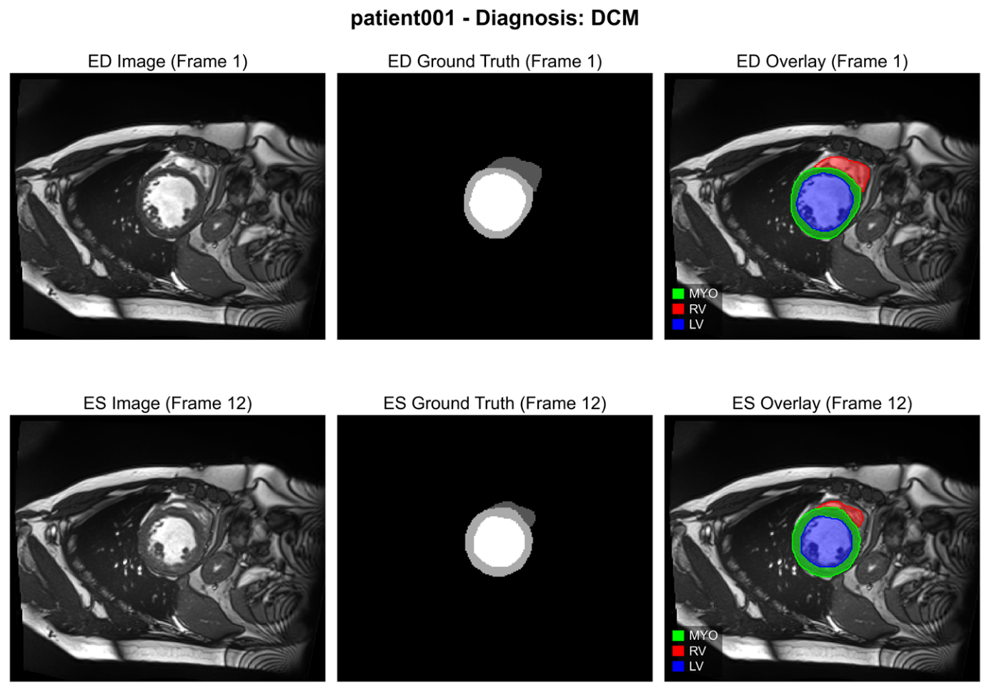
Figure A2.
Confusion matrices of the optimized (a) SVM and (b) random forest classifiers, aggregated over the 25 outer evaluation folds.
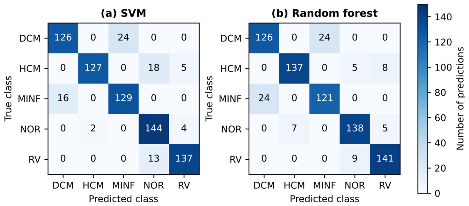
Figure A3.
SHAP feature importance of the CatBoost model for the DCM class (model fitted to the full cohort, n = 149).
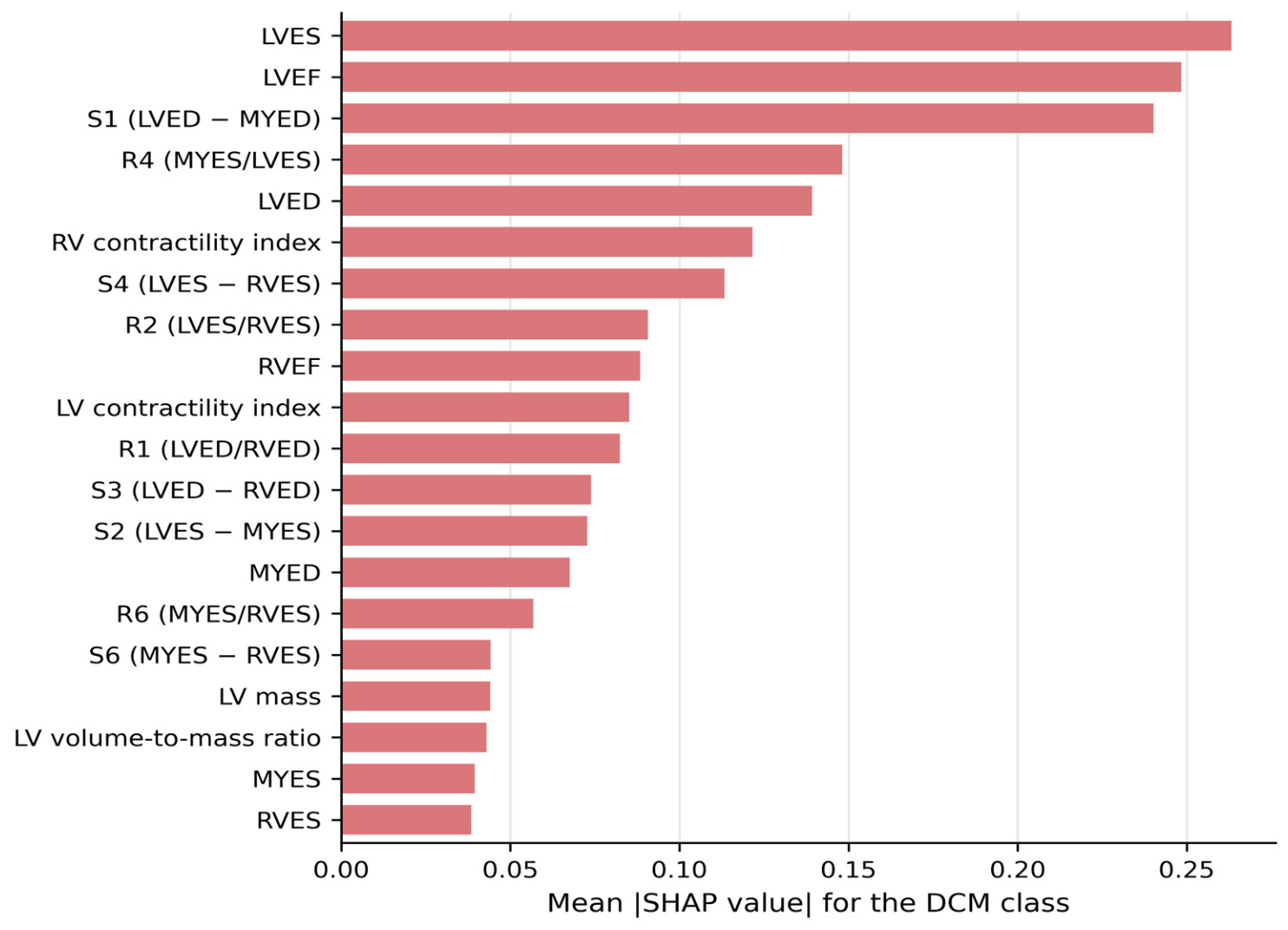
Figure A4.
SHAP feature importance of the CatBoost model for the HCM class (model fitted to the full cohort, n = 149).
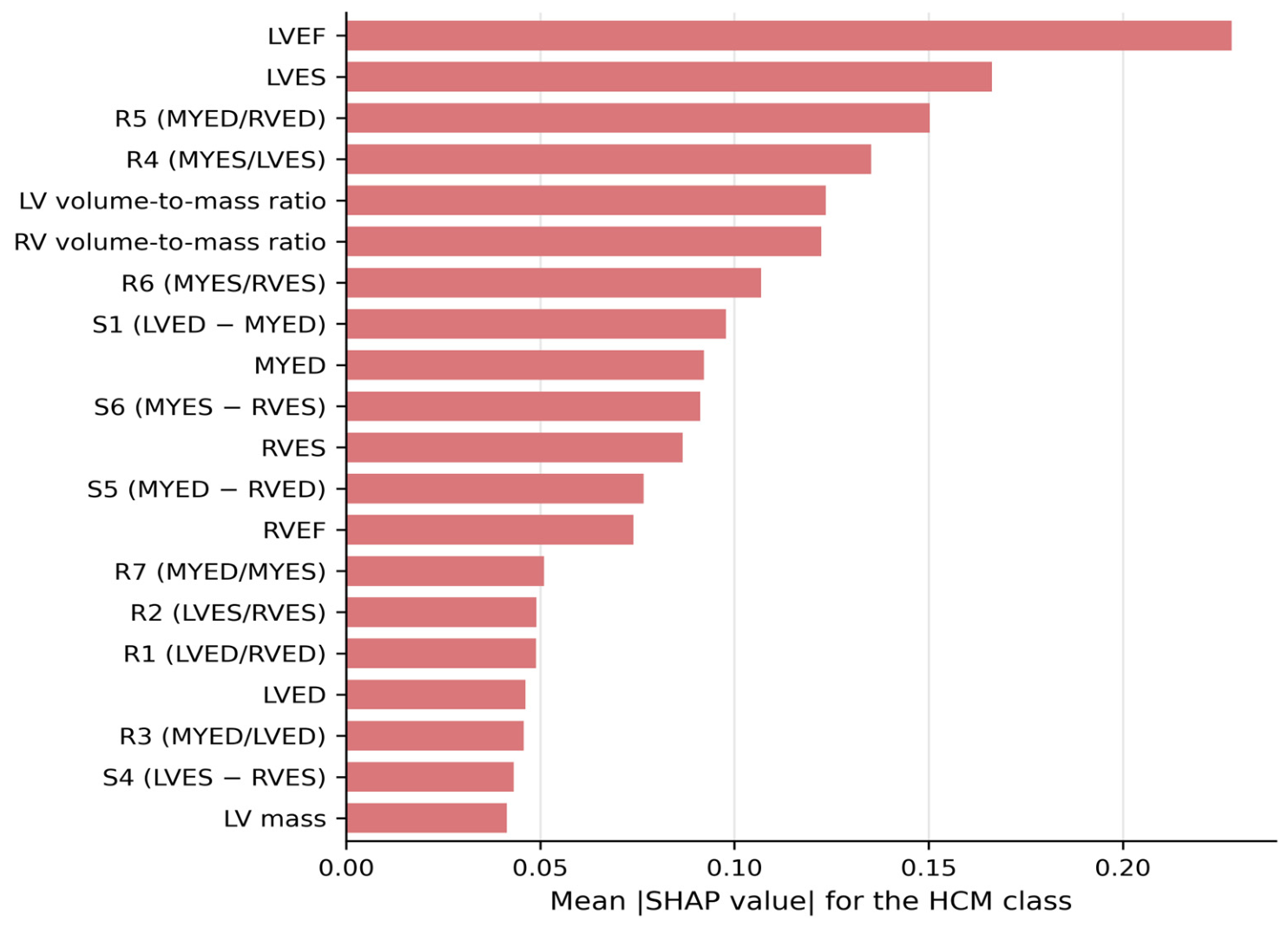
Figure A5.
SHAP feature importance of the CatBoost model for the MINF class (model fitted to the full cohort, n = 149).
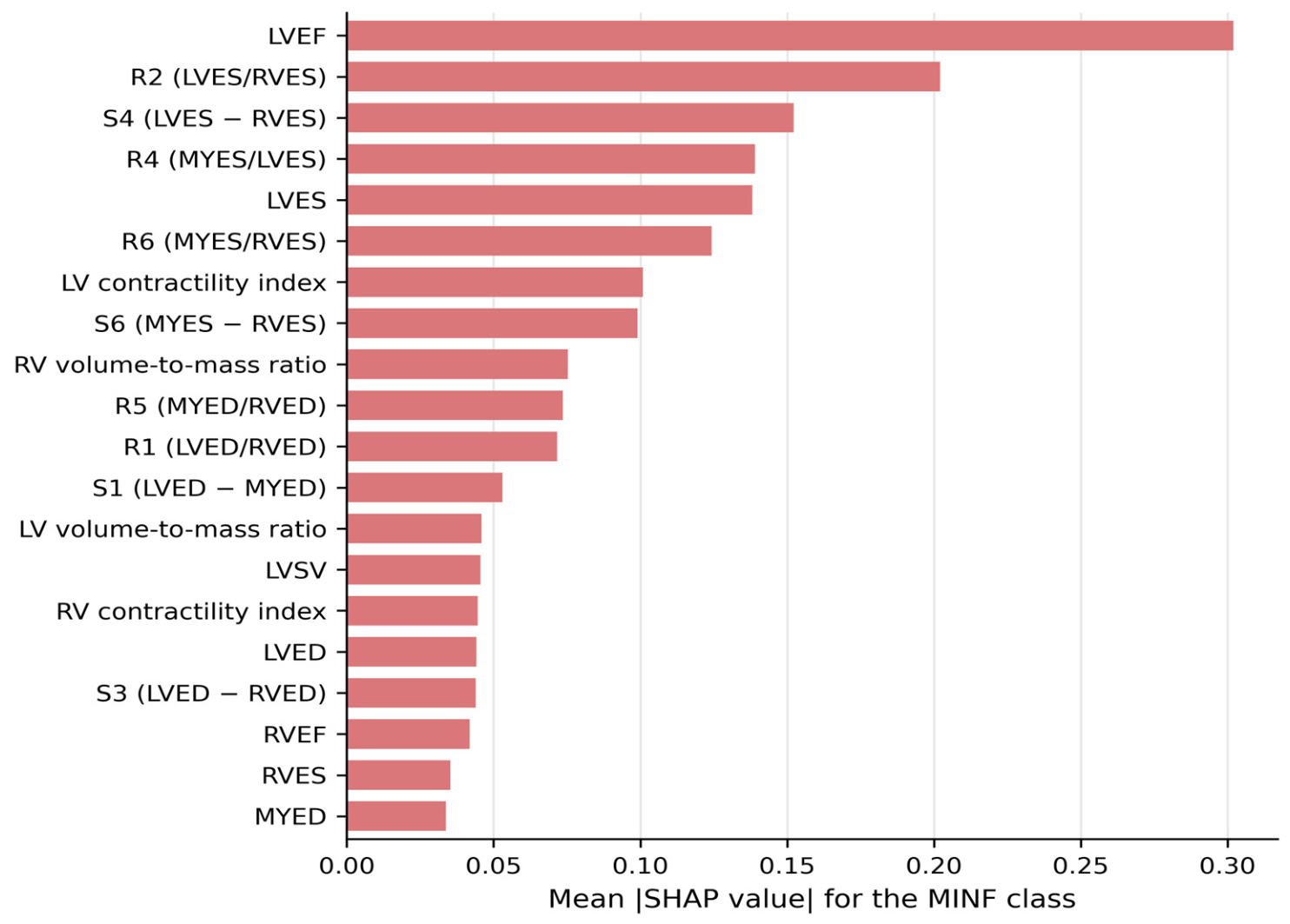
Figure A6.
SHAP feature importance of the CatBoost model for the NOR class (model fitted to the full cohort, n = 149).
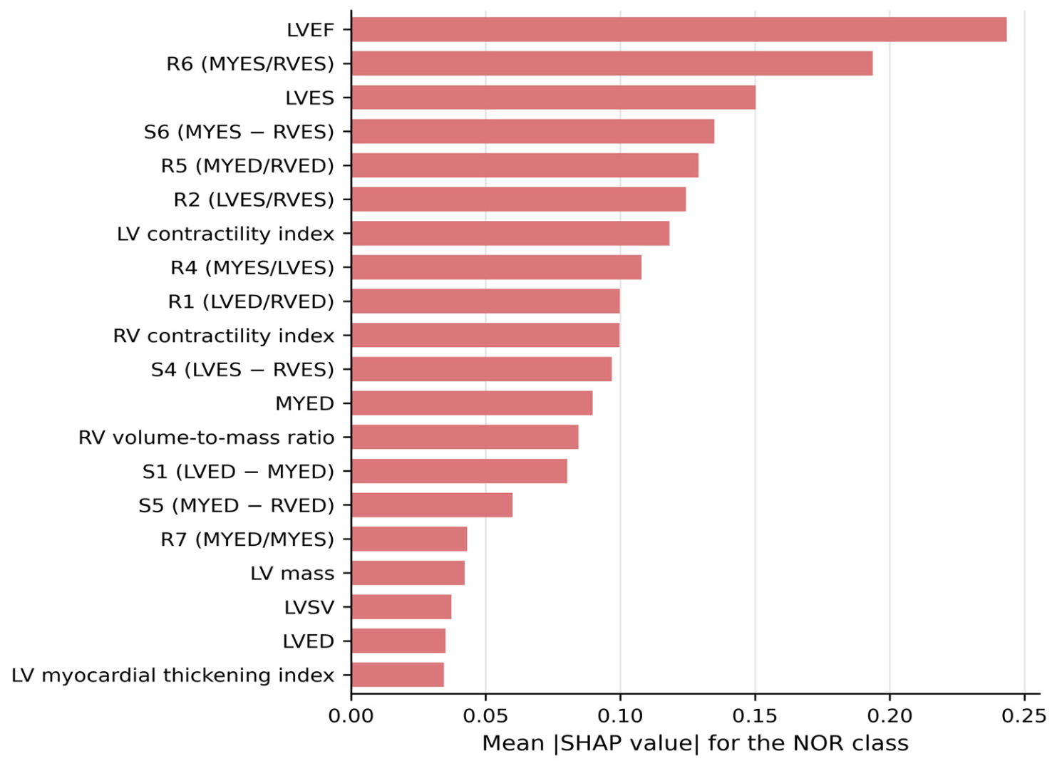
Figure A7.
SHAP feature importance of the CatBoost model for the RV class (model fitted to the full cohort, n = 149).
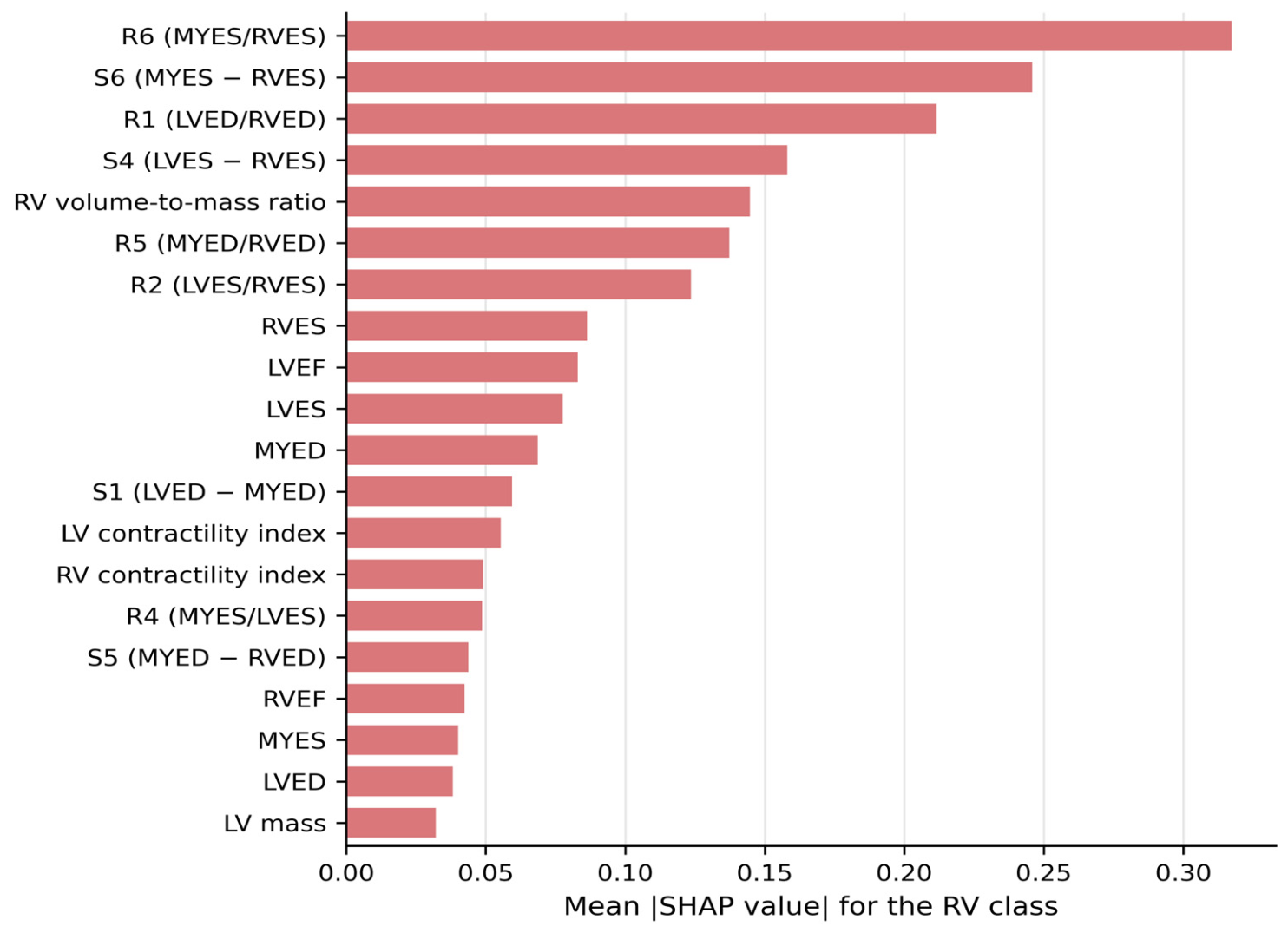
Table A1.
Definitions of the differential (S1-S6), ratio (R1-R7), and extended features derived from the ventricular and myocardial volumes at ED and ES.
Table A2.
Classification performance of the nine classifiers in the baseline configuration (weighted-ensemble biomarkers, n = 149; mean across the 25 outer folds).
Table A3.
Ground-truth-derived biomarkers by diagnostic class (mean ± SD [minimum-maximum]) and per-class differences between the weighted-ensemble and ground-truth values (Δ, mean ± SD), n = 149.
Table A4.
Hold-out classification performance: classifiers trained on the biomarkers of the ACDC training patients (ensemble: n = 99; GT: n = 100) and evaluated once on the 50 ACDC test patients. Values: accuracy (%) [95% bootstrap CI]/macro F1 (%). Retraining the GT classifiers on the same 99 patients as the ensemble source yielded identical test accuracies (Section 3.5).
References
- Martin-Isla, C.; Campello, V.M.; Izquierdo, C.; Raisi-Estabragh, Z.; Baeßler, B.; Petersen, S.E.; Lekadir, K. Image-based cardiac diagnosis with machine learning: A review. Front. Cardiovasc. Med. 2020, 7, 1. [Google Scholar] [CrossRef] [Scilit] [PubMed]
- Chen, C.; Qin, C.; Qiu, H.; Tarroni, G.; Duan, J.; Bai, W.; Rueckert, D. Deep learning for cardiac image segmentation: A review. Front. Cardiovasc. Med. 2020, 7, 25. [Google Scholar] [CrossRef] [Scilit] [PubMed]
- Seraphim, A.; Knott, K.D.; Augusto, J.; Bhuva, A.N.; Manisty, C.; Moon, J.C. Quantitative cardiac MRI. J. Magn. Reson. Imaging 2020, 51, 693–711. [Google Scholar] [CrossRef] [Scilit] [PubMed]
- Morales, M.A.; Manning, W.J.; Nezafat, R. Present and future innovations in AI and cardiac MRI. Radiology 2024, 310, e231269. [Google Scholar] [CrossRef] [Scilit] [PubMed]
- Sermesant, M.; Delingette, H.; Cochet, H.; Jaïs, P.; Ayache, N. Applications of artificial intelligence in cardiovascular imaging. Nat. Rev. Cardiol. 2021, 18, 600–609. [Google Scholar] [CrossRef] [Scilit] [PubMed]
- Wijesinghe, C.; Meedeniya, D.; Yogarajah, P. Cardiac MRI segmentation of ventricular structures and myocardium using U-Net variants. In Proceedings of the 2025 International Conference on Advanced Research in Computing (ICARC); IEEE: Piscataway, NJ, USA, 2025; pp. 1–6. [Google Scholar] [CrossRef] [Scilit]
- Bernard, O.; Lalande, A.; Zotti, C.; Cervenansky, F.; Yang, X.; Heng, P.-A.; Cetin, I.; Lekadir, K.; Camara, O.; Ballester, M.A.G.; et al. Deep learning techniques for automatic MRI cardiac multi-structures segmentation and diagnosis: Is the problem solved? IEEE Trans. Med. Imaging 2018, 37, 2514–2525. [Google Scholar] [CrossRef] [Scilit] [PubMed]
- Isensee, F.; Jaeger, P.F.; Full, P.M.; Wolf, I.; Engelhardt, S.; Maier-Hein, K.H. Automatic cardiac disease assessment on cine-MRI via time-series segmentation and domain specific features. In Statistical Atlases and Computational Models of the Heart. ACDC and MMWHS Challenges (STACOM 2017); Lecture Notes in Computer Science; Pop, M., Sermesant, M., Jodoin, P.-M., Lalande, A., Zhuang, X., Yang, G., Young, A., Bernard, O., Eds.; Springer: Cham, Switzerland, 2018; Volume 10663, pp. 120–129. [Google Scholar] [CrossRef] [Scilit]
- Isensee, F.; Jaeger, P.F.; Kohl, S.A.A.; Petersen, J.; Maier-Hein, K.H. nnU-Net: A self-configuring method for deep learning-based biomedical image segmentation. Nat. Methods 2021, 18, 203–211. [Google Scholar] [CrossRef] [Scilit] [PubMed]
- Chen, J.; Lu, Y.; Yu, Q.; Luo, X.; Adeli, E.; Wang, Y.; Lu, L.; Yuille, A.L.; Zhou, Y. TransUNet: Transformers make strong encoders for medical image segmentation. arXiv 2021, arXiv:2102.04306. [Google Scholar] [CrossRef] [Scilit]
- Cao, H.; Wang, Y.; Chen, J.; Jiang, D.; Zhang, X.; Tian, Q.; Wang, M. Swin-Unet: Unet-like pure transformer for medical image segmentation. In Computer Vision—ECCV 2022 Workshops; Lecture Notes in Computer Science; Karlinsky, L., Michaeli, T., Nishino, K., Eds.; Springer: Cham, Switzerland, 2023; Volume 13803, pp. 205–218. [Google Scholar] [CrossRef] [Scilit]
- Snaauw, G.; Gong, D.; Maicas, G.; van den Hengel, A.; Niessen, W.J.; Verjans, J.; Carneiro, G. End-to-end diagnosis and segmentation learning from cardiac magnetic resonance imaging. In Proceedings of the 2019 IEEE International Symposium on Biomedical Imaging (ISBI); IEEE: Piscataway, NJ, USA, 2019; pp. 802–805. [Google Scholar] [CrossRef] [Scilit]
- Bhatia, D.; Kanakatte, A.; Ghose, A. Cardiac anomaly detection from cine MRI images using physiological features and random forest classifier. In Proceedings of the 44th Annual International Conference of the IEEE Engineering in Medicine & Biology Society (EMBC); IEEE: Piscataway, NJ, USA, 2022; pp. 3801–3804. [Google Scholar] [CrossRef] [Scilit] [PubMed]
- Ronneberger, O.; Fischer, P.; Brox, T. U-Net: Convolutional networks for biomedical image segmentation. In Medical Image Computing and Computer-Assisted Intervention—MICCAI 2015; Lecture Notes in Computer Science; Navab, N., Hornegger, J., Wells, W.M., Frangi, A.F., Eds.; Springer: Cham, Switzerland, 2015; Volume 9351, pp. 234–241. [Google Scholar] [CrossRef] [Scilit]
- Alom, M.Z.; Hasan, M.; Yakopcic, C.; Taha, T.M.; Asari, V.K. Recurrent residual convolutional neural network based on U-Net (R2U-Net) for medical image segmentation. arXiv 2018, arXiv:1802.06955. [Google Scholar] [CrossRef] [Scilit]
- Oktay, O.; Schlemper, J.; Le Folgoc, L.; Lee, M.; Heinrich, M.; Misawa, K.; Mori, K.; McDonagh, S.; Hammerla, N.Y.; Kainz, B.; et al. Attention U-Net: Learning where to look for the pancreas. arXiv 2018, arXiv:1804.03999. [Google Scholar] [CrossRef] [Scilit]
- Buslaev, A.; Iglovikov, V.I.; Khvedchenya, E.; Parinov, A.; Druzhinin, M.; Kalinin, A. Albumentations: Fast and flexible image augmentations. Information 2020, 11, 125. [Google Scholar] [CrossRef] [Scilit]
- Kingma, D.P.; Ba, J. Adam: A method for stochastic optimization. In Proceedings of the 3rd International Conference on Learning Representations (ICLR), San Diego, CA, USA, 7–9 May 2015. [Google Scholar] [CrossRef] [Scilit]
- Gan, M.; Xie, W.; Tan, X.; Wang, W. Coronary artery segmentation framework based on three types of U-Net and voting ensembles. Health Inf. Sci. Syst. 2025, 13, 6. [Google Scholar] [CrossRef] [Scilit] [PubMed]
- Schulz-Menger, J.; Bluemke, D.A.; Bremerich, J.; Flamm, S.D.; Fogel, M.A.; Friedrich, M.G.; Kim, R.J.; von Knobelsdorff-Brenkenhoff, F.; Kramer, C.M.; Pennell, D.J.; et al. Standardized image interpretation and post-processing in cardiovascular magnetic resonance—2020 update: Society for Cardiovascular Magnetic Resonance (SCMR): Board of Trustees Task Force on Standardized Post-Processing. J. Cardiovasc. Magn. Reson. 2020, 22, 19. [Google Scholar] [CrossRef] [Scilit] [PubMed]
- Mosteller, R.D. Simplified calculation of body-surface area. N. Engl. J. Med. 1987, 317, 1098. [Google Scholar] [CrossRef] [Scilit] [PubMed]
- Chen, T.; Guestrin, C. XGBoost: A scalable tree boosting system. In Proceedings of the 22nd ACM SIGKDD International Conference on Knowledge Discovery and Data Mining (KDD ‘16); Association for Computing Machinery: New York, NY, USA, 2016; pp. 785–794. [Google Scholar] [CrossRef] [Scilit]
- Prokhorenkova, L.; Gusev, G.; Vorobev, A.; Dorogush, A.V.; Gulin, A. CatBoost: Unbiased boosting with categorical features. In Advances in Neural Information Processing Systems; Curran Associates, Inc.: Red Hook, NY, USA, 2018; Volume 31. [Google Scholar] [CrossRef] [Scilit]
- Uddin, N.; Mahmud, P.; Ahammed, M.; Uddin, M.A.; Kazi, M.; Talukder, M.A. Explainable ensemble learning model for cardiovascular disease prediction with feature optimization and data balancing. Discov. Comput. 2026, 29, 44. [Google Scholar] [CrossRef] [Scilit]
- Nadeau, C.; Bengio, Y. Inference for the generalization error. Mach. Learn. 2003, 52, 239–281. [Google Scholar] [CrossRef] [Scilit]
- Dice, L.R. Measures of the amount of ecologic association between species. Ecology 1945, 26, 297–302. [Google Scholar] [CrossRef] [Scilit]
- Jaccard, P. The distribution of the flora in the alpine zone. New Phytol. 1912, 11, 37–50. [Google Scholar] [CrossRef] [Scilit]
- Huttenlocher, D.P.; Klanderman, G.A.; Rucklidge, W.J. Comparing images using the Hausdorff distance. IEEE Trans. Pattern Anal. Mach. Intell. 1993, 15, 850–863. [Google Scholar] [CrossRef] [Scilit]
- Lundberg, S.M.; Lee, S.-I. A unified approach to interpreting model predictions. In Advances in Neural Information Processing Systems; Curran Associates, Inc.: Red Hook, NY, USA, 2017; Volume 30. [Google Scholar] [CrossRef] [Scilit]
- Avazmohammadi, R.; Soares, J.S.; Li, D.S.; Eperjesi, T.; Pilla, J.; Gorman, R.C.; Sacks, M.S. On the in vivo systolic compressibility of left ventricular free wall myocardium in the normal and infarcted heart. J. Biomech. 2020, 107, 109767. [Google Scholar] [CrossRef] [Scilit] [PubMed]
- Khened, M.; Kollerathu, V.A.; Krishnamurthi, G. Fully convolutional multi-scale residual DenseNets for cardiac segmentation and automated cardiac diagnosis using ensemble of classifiers. Med. Image Anal. 2019, 51, 21–45. [Google Scholar] [CrossRef] [Scilit] [PubMed]
- Cetin, I.; Sanroma, G.; Petersen, S.E.; Napel, S.; Camara, O.; Gonzalez Ballester, M.A.; Lekadir, K. A radiomics approach to computer-aided diagnosis with cardiac cine-MRI. In Statistical Atlases and Computational Models of the Heart. ACDC and MMWHS Challenges (STACOM 2017); Lecture Notes in Computer Science; Pop, M., Sermesant, M., Jodoin, P.-M., Lalande, A., Zhuang, X., Yang, G., Young, A., Bernard, O., Eds.; Springer: Cham, Switzerland, 2018; Volume 10663, pp. 82–90. [Google Scholar] [CrossRef] [Scilit]
- Wolterink, J.M.; Leiner, T.; Viergever, M.A.; Išgum, I. Automatic segmentation and disease classification using cardiac cine MR images. In Statistical Atlases and Computational Models of the Heart. ACDC and MMWHS Challenges (STACOM 2017); Lecture Notes in Computer Science; Pop, M., Sermesant, M., Jodoin, P.-M., Lalande, A., Zhuang, X., Yang, G., Young, A., Bernard, O., Eds.; Springer: Cham, Switzerland, 2018; Volume 10663, pp. 101–110. [Google Scholar] [CrossRef] [Scilit] [PubMed]
- McDonagh, T.A.; Metra, M.; Adamo, M.; Gardner, R.S.; Baumbach, A.; Böhm, M.; Burri, H.; Butler, J.; Čelutkienė, J.; Chioncel, O.; et al. 2021 ESC guidelines for the diagnosis and treatment of acute and chronic heart failure. Eur. Heart J. 2021, 42, 3599–3726. [Google Scholar] [CrossRef] [Scilit] [PubMed]
- Elliott, P.M.; Anastasakis, A.; Borger, M.A.; Borggrefe, M.; Cecchi, F.; Charron, P.; Hagege, A.A.; Lafont, A.; Limongelli, G.; Mahrholdt, H.; et al. 2014 ESC guidelines on diagnosis and management of hypertrophic cardiomyopathy. Eur. Heart J. 2014, 35, 2733–2779. [Google Scholar] [CrossRef] [Scilit] [PubMed]
- Pinto, Y.M.; Elliott, P.M.; Arbustini, E.; Adler, Y.; Anastasakis, A.; Böhm, M.; Duboc, D.; Gimeno, J.; de Groote, P.; Imazio, M.; et al. Proposal for a revised definition of dilated cardiomyopathy, hypokinetic non-dilated cardiomyopathy, and its implications for clinical practice: A position statement of the ESC working group on myocardial and pericardial diseases. Eur. Heart J. 2016, 37, 1850–1858. [Google Scholar] [CrossRef] [Scilit] [PubMed]
- Maceira, A.M.; Prasad, S.K.; Khan, M.; Pennell, D.J. Normalized left ventricular systolic and diastolic function by steady state free precession cardiovascular magnetic resonance. J. Cardiovasc. Magn. Reson. 2006, 8, 417–426. [Google Scholar] [CrossRef] [Scilit] [PubMed]
- Saporta, A.; Gui, X.; Agrawal, A.; Pareek, A.; Truong, S.Q.H.; Nguyen, C.D.T.; Ngo, V.-D.; Seekins, J.; Blankenberg, F.G.; Ng, A.Y.; et al. Benchmarking saliency methods for chest X-ray interpretation. Nat. Mach. Intell. 2022, 4, 867–878. [Google Scholar] [CrossRef] [Scilit]
- Hundley, W.G.; Bluemke, D.A.; Bogaert, J.; Flamm, S.D.; Fontana, M.; Friedrich, M.G.; Grosse-Wortmann, L.; Karamitsos, T.D.; Kramer, C.M.; Nagel, E.; et al. Society for Cardiovascular Magnetic Resonance (SCMR) guidelines for reporting cardiovascular magnetic resonance examinations. J. Cardiovasc. Magn. Reson. 2022, 24, 29. [Google Scholar] [CrossRef] [Scilit] [PubMed]
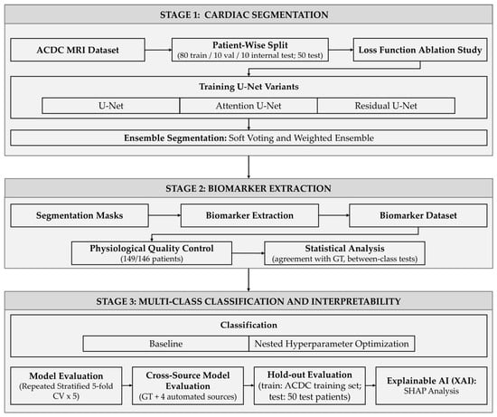
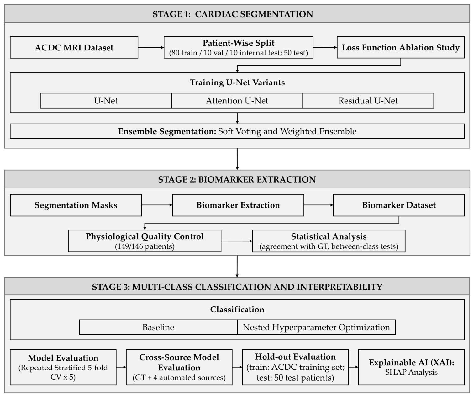
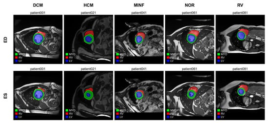
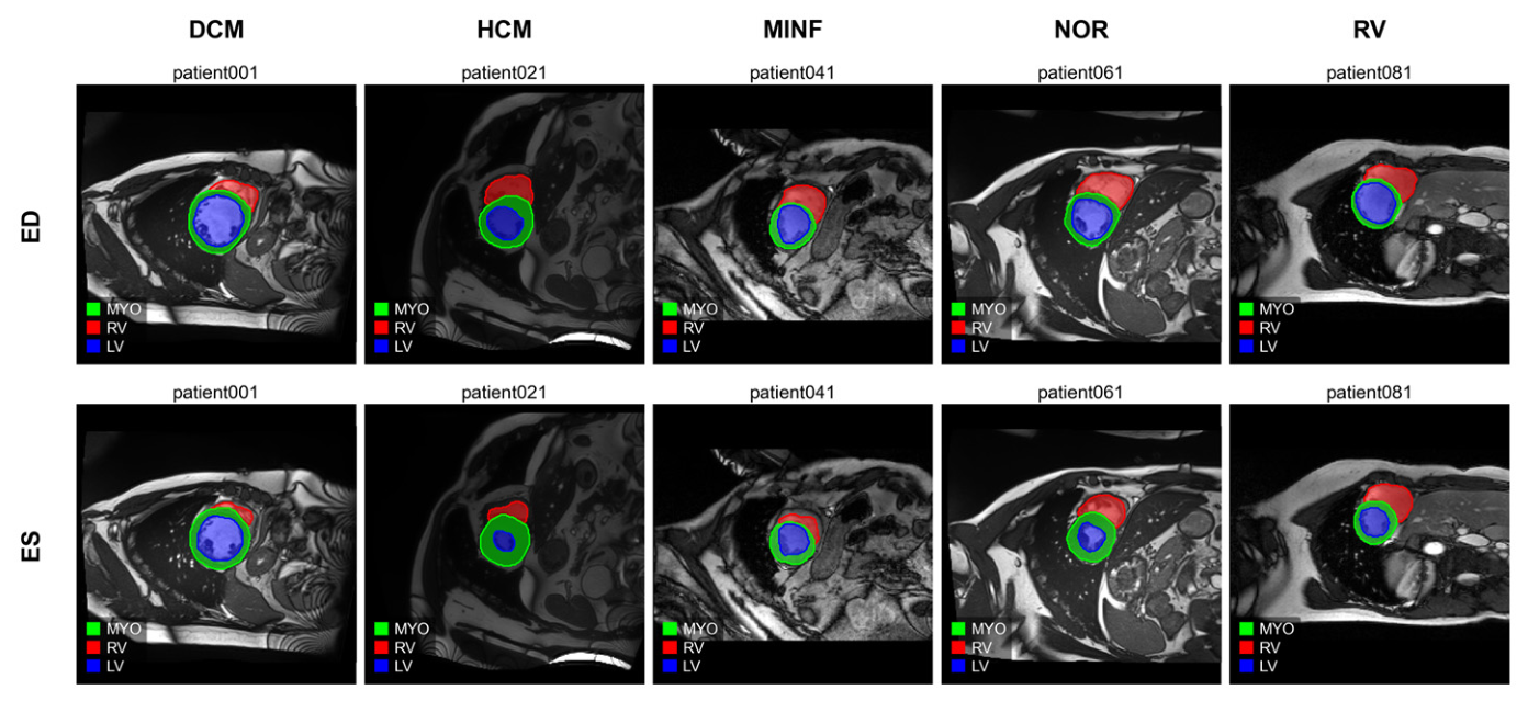
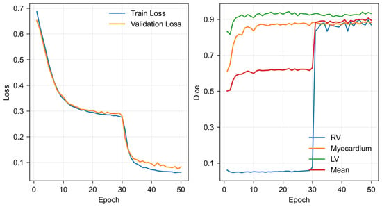
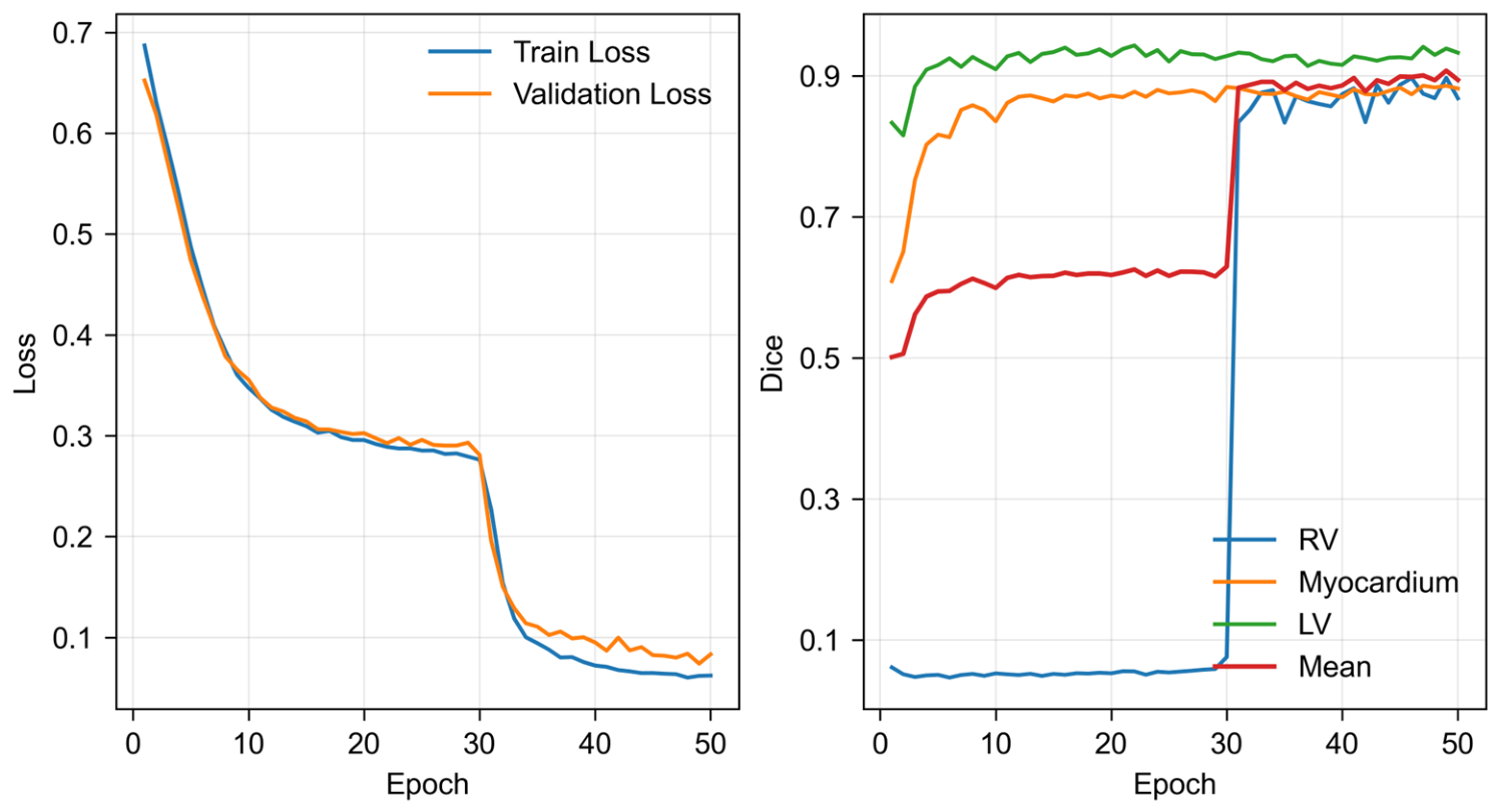
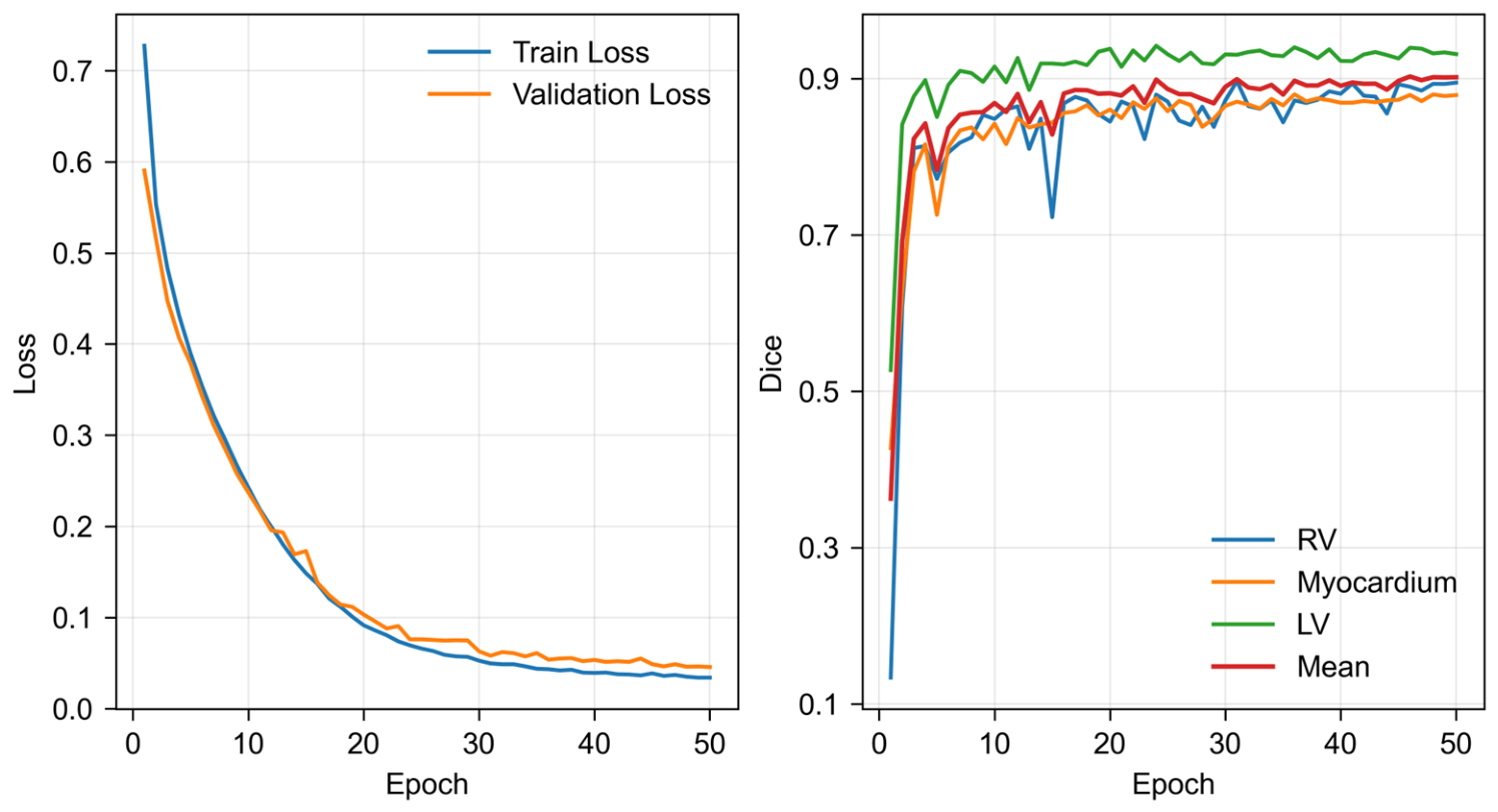
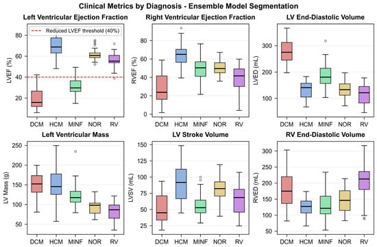
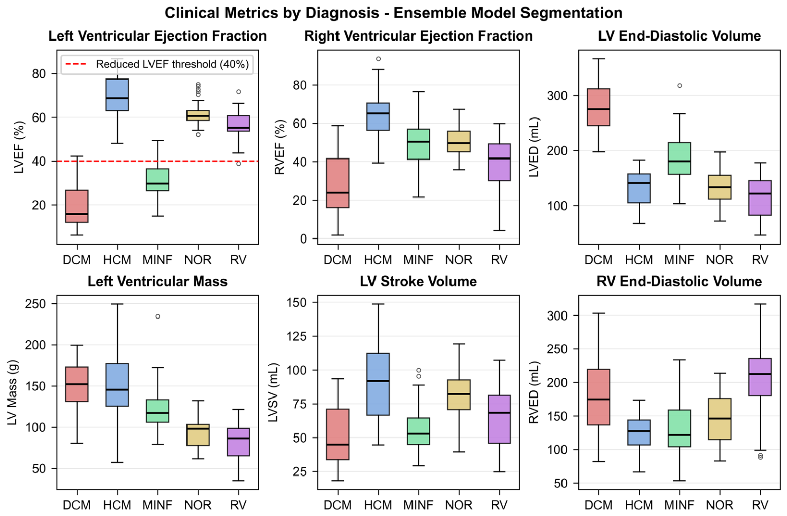
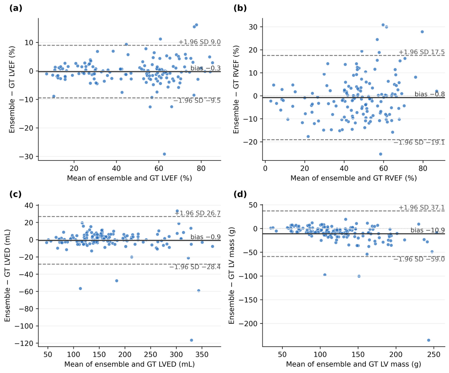
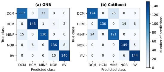
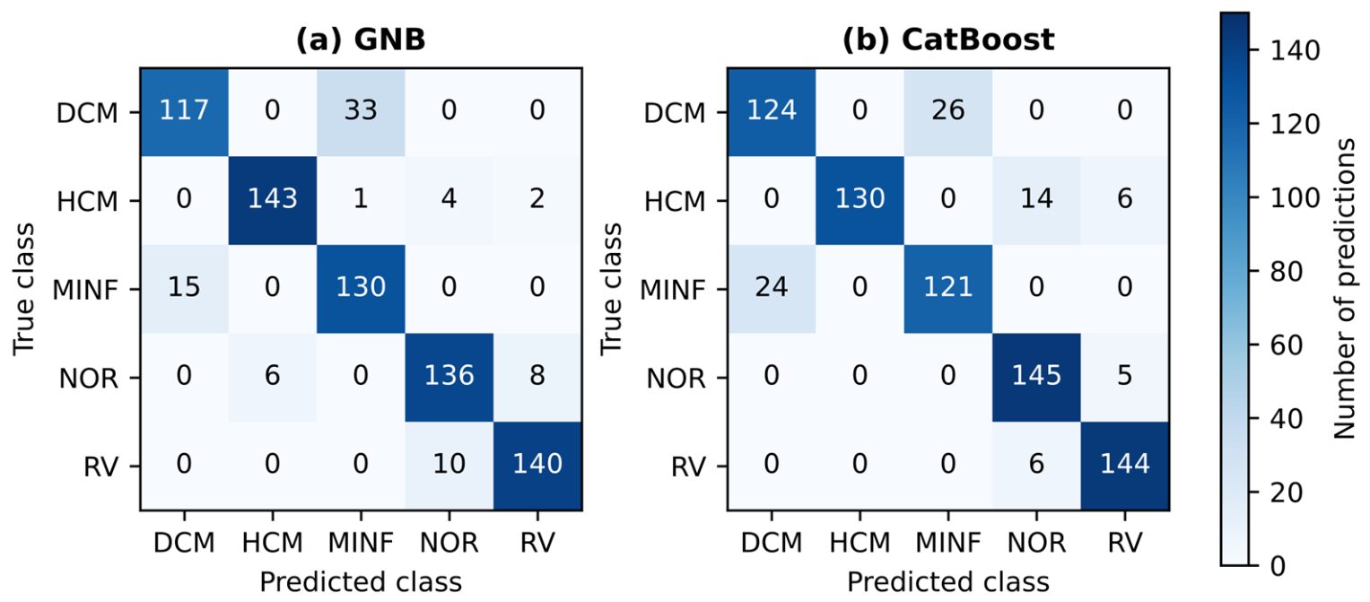
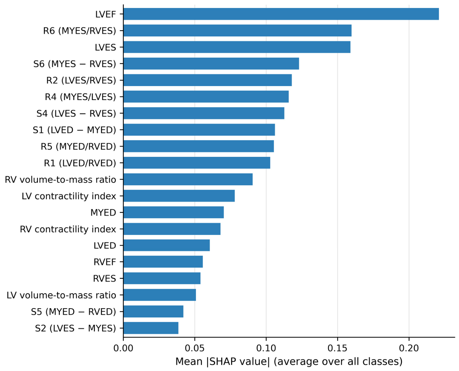

Disclaimer/Publisher’s Note: The statements, opinions and data contained in all publications are solely those of the individual author(s) and contributor(s) and not of MDPI and/or the editor(s). MDPI and/or the editor(s) disclaim responsibility for any injury to people or property resulting from any ideas, methods, instructions or products referred to in the content. |
© 2026 by the authors. Licensee MDPI, Basel, Switzerland. This article is an open access article distributed under the terms and conditions of the Creative Commons Attribution (CC BY) license.