A Robust Online Decision-Making Method Based on DNN Distillation for Energy-Constrained Scenarios in LEO Satellite Passes

Abstract

The rapid motion of Low Earth Orbit (LEO) satellites causes highly time-varying downlink quality, while the radio-frequency energy available during a single pass is strictly limited. Dynamic Programming (DP) optimizes discrete power allocation, but repeated optimization occupies processing capacity shared with other onboard tasks. This motivates compact policies that retain useful transmission performance with lower online computational cost. Hard-label imitation learning neither captures the value similarity among power actions nor guarantees the energy constraint. This paper proposes a lightweight online power-control method based on value-aware policy distillation. DP is used offline to generate complete state–action values, which are converted into soft supervision targets for training a compact neural network. During online inference, energy-feasible action masking removes power levels that exceed the remaining energy budget, thereby ensuring strict constraint satisfaction. The resulting policy observes the actual link and geometric states at each time slot and dynamically reallocates the remaining energy. Simulation results show near-DP average performance under nominal conditions, improvement over hard-label training, and adaptation to signal-to-noise ratio (SNR) forecast errors and along-track ephemeris errors. Rolling cross-level greedy achieves better transmission performance, while the proposed policy uses substantially less CPU time in the tested implementations, illustrating a performance–computation trade-off.

1. Introduction

Low Earth Orbit (LEO) constellations are key to broadband access and non-terrestrial networks, combining wide-area coverage with substantially lower propagation delay than traditional geostationary systems [1,2,3,4]. Their integration with terrestrial networks has driven research on traffic offloading, cooperative transmission, and satellite–terrestrial relaying [5,6]. During a short pass, the satellite’s high relative velocity rapidly changes the slant range and elevation angle, producing strongly time-varying downlink quality. Meanwhile, the radio-frequency (RF) energy available for transmission during a pass is limited by the onboard power budget. Maximizing the transmitted data under this budget therefore requires power decisions that follow the instantaneous link condition and the discrete modulation and coding modes used by systems such as DVB-S2X [7,8]. Online power allocation under these conditions requires balancing transmission performance, computational cost, and adaptation to changing observations.

First, online power allocation shares onboard processing capacity with payload processing, data analysis, and platform control. Reducing the computational workload of power allocation can preserve capacity for these other tasks. The cost of explicit optimization also depends on the state and action spaces and the frequency of replanning. The study in [9] investigated joint access scheduling and subchannel–power allocation for a networked telemetry system of mega-LEO constellations, but its network-wide formulation differs from the cumulative energy allocation problem within a single pass. Ref. [10] used proximal policy optimization for continuous power and bandwidth allocation in multibeam satellites and demonstrated the computational advantage of learned online inference; however, it did not address discrete decisions with adaptive coding and modulation (ACM) under an exact pass-level energy budget. Dynamic Programming (DP) provides an exact offline benchmark for the discretized problem considered here. Distilling its action values into a compact policy offers a way to retain useful throughput with lower online processing cost. Learning-based optimization approximations and deep reinforcement learning (DRL) offer ways to shift substantial computation to offline policy construction [11,12,13,14].

Second, a learned policy must preserve decision quality and physical feasibility. The work in [8] investigated online DRL-based power allocation for multibeam satellites, while [14] jointly optimized beam patterns and bandwidth through multi-agent DRL. These studies support low-latency learned resource management, but they target multi-beam traffic matching rather than distilling an exact DP solution for a finite-energy pass. The study in [15] further combined a deep Q-network (DQN) for discrete resource allocation with proximal policy optimization for continuous power control in a LEO satellite–terrestrial network based on rate-splitting multiple access, illustrating the difficulty of mixed discrete–continuous decisions. It did not, however, use state–action values as soft supervision or impose a pass-level cumulative energy constraint through exact action masking. Related work on general wireless networks has likewise shown that multi-agent DRL can provide low-latency power control from local observations [16]. Nevertheless, directly encoding only the single optimal discrete action as a one-hot target discards the relative values of the remaining actions. In the stepwise throughput response induced by ACM, such hard-label training penalizes a near-optimal action and a zero-throughput action in the same way. Moreover, unconstrained network outputs cannot guarantee energy feasibility during sequential inference unless explicitly enforced.

Finally, a static offline schedule is sensitive to discrepancies between predicted and observed link states. The study in [17] developed a stochastic rain-attenuation model that explicitly accounts for the changing elevation angle of LEO links above 10 GHz, providing physical support for evaluating time-varying signal-to-noise ratio (SNR) rather than assuming a fixed attenuation margin. At the network layer, the work in [18] investigated distributed link management under mobility, traffic variation, and link failures, further demonstrating the need to adapt decisions to current network observations. These studies model important sources of link and topology dynamics, whereas the present work focuses on how a lightweight power-control policy responds online when forecast SNR and pass geometry differ from their nominal values. Such discrepancies can shift the time slots in which an ACM threshold is crossed. A one-shot schedule computed from an imperfect forecast may then spend scarce energy in low-yield slots, whereas an online policy can update its decisions from the measured geometry and SNR.

To address these trade-offs, this paper proposes a compact deep neural network (DNN) framework for energy-constrained downlink power control during a single LEO pass. The goal is to reduce online processor occupation while preserving transmission performance, energy feasibility, and adaptation to observed link changes. The framework (i) moves DP teacher computation and policy training offline and uses fixed-size neural inference online, achieving near-DP average performance under nominal test conditions; (ii) distills the complete DP action-value table into soft supervision targets and applies energy-feasible action masking to enforce the energy budget exactly; and (iii) uses observed geometry and SNR for online energy reallocation under forecast errors and along-track ephemeris errors. The comparison with rolling cross-level greedy explicitly evaluates the transmission loss incurred in exchange for lower online computation.

2. System Model and Problem Formulation

2.1. LEO Pass Geometry and Visible Window

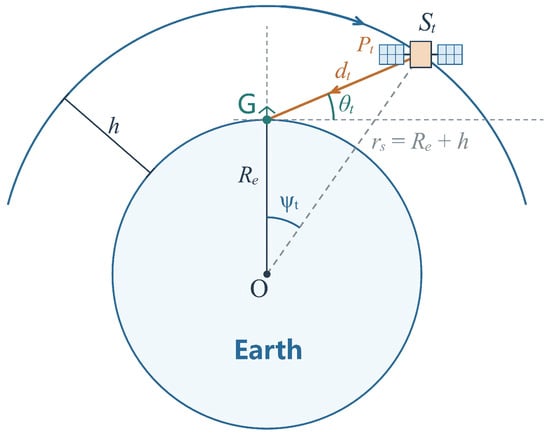
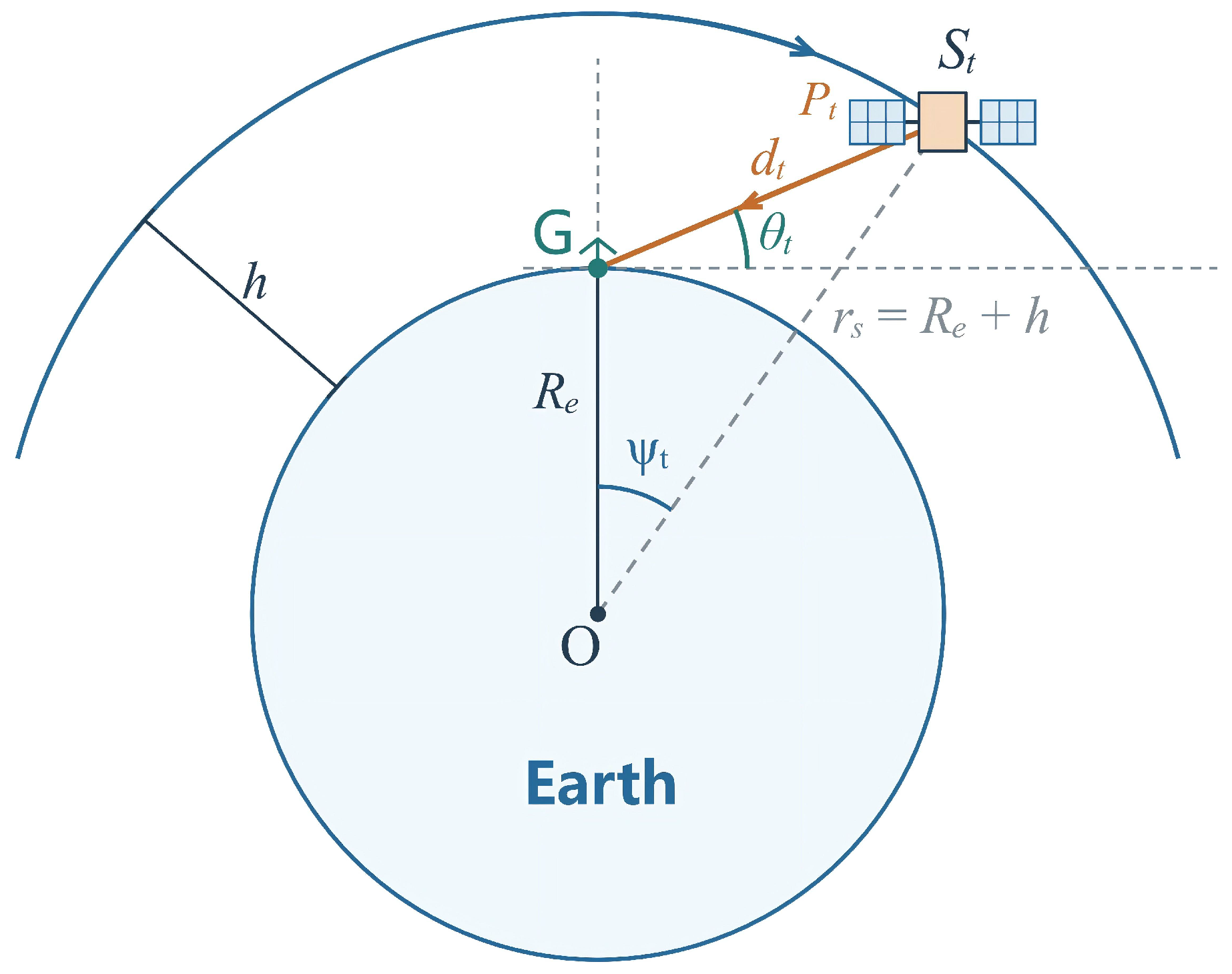
As shown in Figure 1, a LEO satellite transmits data to a fixed ground station during a single pass. As the satellite approaches and recedes from the station, its slant range and elevation angle vary continuously, leading to time-varying link quality and achievable data rates. Transmission power is therefore allocated across the visible window to maximize the transmitted data under a total energy budget.

Figure 1. Illustration of the LEO satellite pass downlink communication scenario.

To characterize the satellite-ground geometry, we adopt a circular-orbit approximation and neglect Earth rotation during the several-minute pass.

The usable pass window is divided into N equal time slots indexed by $t\in \mathcal{T}=\{0,1,\dots ,N-1\}$. Within $\Delta t$, the satellite position, propagation loss, and transmission power are treated as static. Given the Earth radius $R_E$ and orbital altitude h, the orbital radius is $r_s=R_E+h$ and the angular velocity is $\omega =\sqrt{\mu /r_s^3}$, where $\mu$ is the Earth’s gravitational parameter.

Using an Earth-centered Cartesian frame, let $\tau =0$ denote closest approach. The satellite and ground-station unit position vectors are $\mathit{s}\left(\tau \right)={[\cos \left(\omega \tau \right),\sin \left(\omega \tau \right),0]}^{\mathsf{T}}$ and $\mathit{g}={[\cos {\psi }_0,0,\sin {\psi }_0]}^{\mathsf{T}}$, where ${\psi }_0$ is the closest-approach geocentric angle. Here, ${\psi }_0=0$ represents a zenith pass, while larger values indicate greater trajectory deviation and a lower maximum elevation.

With ${\mathit{r}}_s\left(\tau \right)=r_s\mathit{s}\left(\tau \right)$ and ${\mathit{r}}_g=R_E\mathit{g}$, the dynamic geocentric angle satisfies $\cos \psi \left(\tau \right)=\cos {\psi }_0\cos \left(\omega \tau \right)$. The line-of-sight vector is $\mathit{\ell }\left(\tau \right)={\mathit{r}}_s\left(\tau \right)-{\mathit{r}}_g$, and its length is the slant range $d\left(\tau \right)={\parallel \mathit{\ell }\left(\tau \right)\parallel }_2$. By the law of cosines,

$$\begin{array}{c}\hfill d\left(\tau \right)=\sqrt{r_s^2+R_E^2-2r_s{R}_E\cos \psi \left(\tau \right)}.\end{array}$$

(1)

The elevation angle $\theta \left(\tau \right)$ is measured between the line of sight and the local horizontal plane, so $\sin \theta \left(\tau \right)={\mathit{\ell }}^{\mathsf{T}}\left(\tau \right)\mathit{g}/d\left(\tau \right)$. Therefore,

$$\theta \left(\tau \right)=\arcsin \left[{\displaystyle \frac{r_s\cos \psi \left(\tau \right)-R_E}{d\left(\tau \right)}}\right].$$

(2)

To avoid severe atmospheric attenuation and ground occlusion, a minimum working elevation ${\theta }_{\min }$ is imposed and communication requires $\theta \left(\tau \right)\ge {\theta }_{\min }$. From $\tan \theta =(r_s\cos \psi -R_E)/\left(r_s\sin \psi \right)$, the boundary geocentric angle is

$${\psi }_{\mathrm{vis}}=\arccos \left({\displaystyle \frac{R_E}{r_s}}\cos {\theta }_{\min }\right)-{\theta }_{\min }.$$

(3)

If ${\psi }_0\le {\psi }_{\mathrm{vis}}$, the pass is effective. Its exit time follows from $\psi \left({\tau }_{\mathrm{out}}\right)={\psi }_{\mathrm{vis}}$ as

$$\begin{array}{c}\hfill {\tau }_{\mathrm{out}}={\displaystyle \frac{1}{\omega }}\arccos \left({\displaystyle \frac{\cos {\psi }_{\mathrm{vis}}}{\cos {\psi }_0}}\right).\end{array}$$

(4)

The entry time is ${\tau }_{\mathrm{in}}=-{\tau }_{\mathrm{out}}$ and the pass duration is $T_{\mathrm{pass}}=2{\tau }_{\mathrm{out}}$. Sampling by $\Delta t$ gives $\lfloor T_{\mathrm{pass}}/\Delta t\rfloor$ centered slots, with slot midpoint ${\tau }_t=(t+1/2)\Delta t-N\Delta t/2$. Here, $d_t=d\left({\tau }_t\right)$ and ${\theta }_t=\theta \left({\tau }_t\right)$ denote the slant range and elevation angle in slot t.

2.2. Link Budget and Received SNR

The link loss in slot t consists of four terms. The free-space path loss $L_{\mathrm{FS},t}$ is

$$\begin{array}{c}\hfill L_{\mathrm{FS},t}=20{\log }_{10}\left({\displaystyle \frac{4\pi f_c{d}_t}{c}}\right),\end{array}$$

(5)

where $f_c$ is the carrier frequency and c is the speed of light in a vacuum. Second, as the thickness of the Earth’s atmosphere traversed by electromagnetic waves increases significantly with a decrease in elevation angle, the resulting elevation-dependent atmospheric attenuation $A_{\mathrm{atm},t}$ is modeled as

$$\begin{array}{c}\hfill A_{\mathrm{atm},t}={\displaystyle \frac{A_{\mathrm{zen}}}{\max \{\sin {\theta }_t,\sin {\theta }_{\min }\}}},\end{array}$$

(6)

where $A_{\mathrm{zen}}$ is the zenith atmospheric attenuation. The remaining terms are weather-induced attenuation $A_{\mathrm{w}}$ and a fixed miscellaneous loss $L_{\mathrm{misc}}$ for feeder, implementation, and pointing errors, giving $L_{\mathrm{tot},t}=L_{\mathrm{FS},t}+A_{\mathrm{atm},t}+A_{\mathrm{w}}+L_{\mathrm{misc}}$.

To reflect finite hardware control, the transmit power $P_t$ is restricted to $\mathcal{P}=\{P^{\left(0\right)},P^{\left(1\right)},\dots ,P^{(A-1)}\}$, where $P^{\left(0\right)}=0$ denotes silence. With antenna gains $G_t$ and $G_r$, the DVB-S2X symbol-energy-to-noise-power-spectral-density ratio is

$$\begin{array}{c}\hfill {\gamma }_t\left(P_t\right)=10{\log }_{10}{P}_t+G_t+G_r-L_{\mathrm{tot},t}-10{\log }_{10}\left(k{T}_{\mathrm{sys}}\right)-10{\log }_{10}{R}_s,\end{array}$$

(7)

where k is the Boltzmann constant and $T_{\mathrm{sys}}$ is the receiver system noise temperature.

The dB budget corresponds to the equivalent complex-baseband model. With the power-independent link gain $g_t={10}^{(G_t+G_r-L_{\mathrm{tot},t})/10}$, the received sample after matched filtering and symbol sampling is

$$\begin{array}{c}\hfill y_{t,n}=\sqrt{g_t{E}_{s,t}}{x}_{t,n}+w_{t,n},\end{array}$$

(8)

where $x_{t,n}$ is the normalized transmitted symbol, $E_{s,t}=P_t/R_s$ is the average symbol energy, and $w_{t,n}\sim \mathcal{CN}(0,N_0)$ is complex Gaussian noise with $N_0=k{T}_{\mathrm{sys}}$. Thus, geometry determines the channel gain $g_t$, while power control determines $E_{s,t}$.

To decouple channel quality from the current action, a fixed reference power $P_{\mathrm{ref}}>0$ defines the reference SNR ${\gamma }_t^{\mathrm{ref}}$. For $P_t>0$, the actual SNR is ${\gamma }_t\left(P_t\right)={\gamma }_t^{\mathrm{ref}}+10{\log }_{10}(P_t/P_{\mathrm{ref}})$.

2.3. DVB-S2X Style ACM and Data Rate Model

The system supports a set of modulation and coding (MODCOD) schemes indexed by $\mathcal{M}=\{1,2,\dots ,M\}$. For mode $m\in \mathcal{M}$, ${\eta }_m$ is the maximum net spectral efficiency and ${\Gamma }_m^{\mathrm{ideal}}$ is the ideal switching threshold. With link margin $M_{\mathrm{link}}$, the operating threshold is ${\Gamma }_m={\Gamma }_m^{\mathrm{ideal}}+M_{\mathrm{link}}$.

For $P_t>0$, the feasible mode set is

$$\begin{array}{c}\hfill {\mathcal{M}}_t\left(P_t\right)=\left\{m\in \mathcal{M}:{\gamma }_t\left(P_t\right)\ge {\Gamma }_m\right\}.\end{array}$$

(9)

When the set is non-empty, the system selects $m_t^{\ast }\left(P_t\right)=\arg {\max }_{m\in {\mathcal{M}}_t\left(P_t\right)}{\eta }_m$; an empty set indicates outage. The achievable rate is

$$\begin{array}{c}\hfill R_t\left(P_t\right)=\left\{\begin{array}{cc}0,\hfill & P_t=0\mathrm{or}{\mathcal{M}}_t\left(P_t\right)=⌀,\hfill \\ R_s{\eta }_{m_t^{\ast }\left(P_t\right)},\hfill & \mathrm{otherwise}.\hfill \end{array}\right.\end{array}$$

(10)

The delivered data per slot is $D_t\left(P_t\right)=R_t\left(P_t\right)\Delta t$, which defines the throughput contribution used in policy optimization.

2.4. Energy-Constrained Power Control Problem

Since all slots share the pass-level energy budget, we formulate the global discrete optimization problem as follows.

Let $E_{\max }$ be the total RF energy budget for the pass. The resulting problem is

$$\begin{array}{c}\hfill \begin{array}{cc}\hfill \mathbf{P}\mathbf{1}:\underset{{\left\{P_t\right\}}_{t=0}^{N-1}}{\max }& D_{\mathrm{total}}={\displaystyle \sum _{t=0}^{N-1}}{D}_t\left(P_t\right)\hfill \\ \hfill \mathrm{s}.\mathrm{t}.& {\displaystyle \sum _{t=0}^{N-1}}{P}_t\Delta t\le E_{\max },\hfill \\ \hfill & P_t\in \mathcal{P},t\in \mathcal{T}.\hfill \end{array}\end{array}$$

(11)

Because each slot return depends only on the current link state while all actions share one budget, P1 is a multiple-choice knapsack problem. For DP, let the candidate powers be equally spaced as $P^{\left(a\right)}=a\Delta P,a\in \{0,1,\dots ,A-1\}$. Then the unit energy is $\Delta E=\Delta P\Delta t$, the integer budget is $B=\lfloor E_{\max }/\Delta E\rfloor$, and the cost of action a is $c_a=a$.

3. Dynamic Programming Solution

The optimization problem is a multi-stage sequential decision process with a total resource constraint. Since the pass geometry and large-scale atmospheric attenuation are predictable before the pass and the remaining energy evolves as a one-dimensional state, this section applies DP. Besides providing the exact optimal policy for the discrete model, DP generates the complete state–action value table used to supervise policy distillation.

3.1. Value Recursion and Optimal Policy Recovery

At the beginning of slot t, the state is represented by the remaining energy units b, where $0\le b\le B$. Let $V_t\left(b\right)$ denote the maximum cumulative data that can be transmitted from slot t to the end of the pass with b energy units remaining. The terminal condition is $V_N\left(b\right)=0$.

In state $(t,b)$, the set of feasible actions is restricted by the remaining energy constraint, denoted as $\mathcal{A}\left(b\right)=\{a\in \mathcal{A}:c_a\le b\}$. If the system chooses action $a\in \mathcal{A}\left(b\right)$ in the current state, it obtains an immediate data volume return $D_t\left(a\right)$, and the remaining energy for the next time slot is updated to $b-c_a$. The cumulative action value corresponding to this action is expressed as

$$\begin{array}{c}\hfill Q_t(b,a)=D_t\left(a\right)+V_{t+1}(b-c_a),\end{array}$$

(12)

where $Q_t(b,a)$ is the cumulative action value of taking action a in state $(t,b)$, $D_t\left(a\right)$ is the immediate data volume return of action a, $V_{t+1}(b-c_a)$ is the optimal cumulative value after transitioning to the next state, and $c_a$ is the energy cost of action a.

To ensure global optimality, the maximum value of the current state depends on the maximum cumulative value among all feasible actions. The Bellman recursion is therefore written as

$$\begin{array}{c}\hfill V_t\left(b\right)=\underset{a\in \mathcal{A}\left(b\right)}{\max }\left[D_t\left(a\right)+V_{t+1}(b-c_a)\right],\end{array}$$

(13)

The algorithm performs backward recursion from slot $N-1$ to slot 0 and records the optimal action at each state as

$$\begin{array}{c}\hfill a_t^{\ast }\left(b\right)=\arg \underset{a\in \mathcal{A}\left(b\right)}{\max }{Q}_t(b,a),\end{array}$$

(14)

where $a_t^{\ast }\left(b\right)$ is the optimal decision action under state $(t,b)$.

After completing the reverse calculation, the entire policy table and value table are constructed. Subsequently, starting from the initial state $(0,B)$, the algorithm executes the optimal action $a_0^{\mathrm{DP}}$ and sequentially recovers the complete optimal power sequence ${\mathit{a}}^{\mathrm{DP}}=[a_0^{\mathrm{DP}},a_1^{\mathrm{DP}},\dots ,a_{N-1}^{\mathrm{DP}}]$ through forward iteration $b_{t+1}=b_t-c_{a_t^{\mathrm{DP}}}$. The optimal solution of the initial state is the maximum total data transmission volume of this pass, $D_{\mathrm{DP}}=V_0\left(B\right)$.

3.2. Computational Complexity

For an action space of size A, N time slots, and B energy states, one full-horizon DP solve has time complexity $\mathcal{O}\left(NBA\right)$. More time slots, a finer energy grid, or more frequent replanning increase the work assigned to power allocation. The proposed method moves teacher solution generation and policy training offline; online, a fixed-size network and action mask replace repeated optimization. This reduces the decision workload and can leave more processing capacity available for other onboard tasks while accepting an approximation loss in transmission performance.

For a fully connected inference network with L weight layers and layer widths $n_0,\dots ,n_L$, where $n_L=A$, one decision requires ${\sum }_{\mathcal{l}=1}^L{n}_{\mathcal{l}-1}{n}_{\mathcal{l}}$ multiply–accumulate operations (MACs), together with bias additions and hidden-layer activations. Energy-feasible action masking and maximum selection each require $\mathcal{O}\left(A\right)$ operations. The overall per-slot complexity is therefore $\mathcal{O}({\sum }_{\mathcal{l}=1}^L{n}_{\mathcal{l}-1}{n}_{\mathcal{l}}+A)$. With the architecture and action set fixed, the computational cost over a complete pass grows linearly with N, without a search over the B energy states.

4. Value-Aware Lightweight Neural Network Power Control

To reduce the online computational workload of power decisions, this section trains a neural network on data generated by dynamic programming. Unlike conventional hard-label imitation learning, it converts the complete action-value table into soft supervision signals. Combined with online energy-feasible action masking, this yields a compact decision architecture with fast inference and strict energy-constraint satisfaction.

4.1. Pass Scenario Generation and Network State

To train the network and ensure consistency in feature distribution, a complete satellite pass trajectory is recorded as one episode. The i-th episode generated has a set of parameters characterizing the scenario differences: ${\mathit{\xi }}_i=[h_i,{\psi }_{0,i},E_{\max ,i},A_{\mathrm{w},i}]$. According to the model evolution in Section 2, each scenario produces a unique per-slot throughput profile and is solved by DP.

During online decision-making, the network input for the t-th time slot is constructed from the key state features as

$$\begin{array}{c}\hfill {\mathit{x}}_t={\left[{\overline{\theta }}_t,s_t,{\overline{\gamma }}_t^{\mathrm{ref}},e_t,\zeta ,{\rho }_t,\overline{h},{\overline{\theta }}_{\max }\right]}^{\mathsf{T}},\end{array}$$

(15)

where ${\overline{\theta }}_t$ is the normalized elevation angle reflecting the current geometric position, $s_t$ is the sign variable indicating the direction of elevation angle change, ${\overline{\gamma }}_t^{\mathrm{ref}}$ is the normalized scalar of reference channel quality, $e_t$ is the normalized remaining energy, $\zeta$ is the initial budget intensity, ${\rho }_t$ is the proportion of remaining time reflecting the time progress, $\overline{h}$ is the orbit altitude parameter, and ${\overline{\theta }}_{\max }$ is the maximum elevation angle parameter of the entire pass.

The geometric features use ${\overline{\theta }}_t={\theta }_t/{90}^{\circ }$ and ${\overline{\theta }}_{\max }={\theta }_{\max }/{90}^{\circ }$, where ${\theta }_t$ and ${\theta }_{\max }$ are the current and maximum pass elevations, respectively, expressed in degrees. The direction feature is $s_t=+1$ for ${\tau }_t\le 0$ and $s_t=-1$ for ${\tau }_t>0$, where ${\tau }_t$ is the slot midpoint time relative to closest approach. These signs denote the approaching and receding portions of the pass, with closest approach assigned $+1$; no further scaling is applied. The reference SNR, expressed in dB at the fixed reference power $P_{\mathrm{ref}}$, is standardized as ${\overline{\gamma }}_t^{\mathrm{ref}}=({\gamma }_t^{\mathrm{ref}}-{\mu }_{\gamma })/{\sigma }_{\gamma }$.

The energy features are $e_t=b_t/\max \{B,1\}$ and $\zeta =(B\Delta E)/(N\Delta t{P}_{\max })$. Here, $b_t$ and B are the remaining and initial budgets in discrete energy units, $\Delta E$ is the energy per unit in joules, and $B\Delta E$ is the effective initial RF energy. The maximum available power is $P_{\max }=\max \mathcal{P}$, expressed in watts. The remaining-time feature is ${\rho }_t=(N-1-t)/\max \{N-1,1\}$, where $t\in \{0,\dots ,N-1\}$ is the slot index, N is the number of modeled slots, and $\Delta t$ is the slot duration in seconds; thus, $N\Delta t$ is the modeled pass duration. The maximum operations in the denominators of $e_t$ and ${\rho }_t$ prevent division by zero for a zero discrete budget or a single-slot pass.

Finally, altitude is normalized as $\overline{h}=(h_{\mathrm{km}}-h_{\min }^{\mathrm{tr}})/(h_{\max }^{\mathrm{tr}}-h_{\min }^{\mathrm{tr}})$, where $h_{\mathrm{km}}$ is the orbital altitude in kilometers and $h_{\min }^{\mathrm{tr}}$ and $h_{\max }^{\mathrm{tr}}$ are the minimum and maximum training-pass altitudes in the same units. The superscript $\mathrm{tr}$ denotes the training split.

The SNR mean ${\mu }_{\gamma }$ and population standard deviation ${\sigma }_{\gamma }$ are fitted using one reference-SNR observation per original slot of each training pass, without repeated weighting from additional energy-state samples. The altitude extrema $h_{\min }^{\mathrm{tr}}$ and $h_{\max }^{\mathrm{tr}}$ also come exclusively from training passes. For the original training split, these values are approximately $2.170485$ dB, $3.734666$ dB, $500.195583$ km, and $799.811957$ km, respectively. These parameters are frozen and reused for validation, testing, online inference, and low-budget mixed retraining. Validation and test features are not clipped to the training range.

4.2. Value-Aware Supervision and Lightweight Network Training

Conventional imitation learning uses the DP-optimal action $a_t^{\ast }$ as a one-hot training target. However, under the stepwise ACM throughput response, different power levels may produce the same or similar cumulative returns. One-hot targets do not distinguish among nonselected actions, even when some have cumulative returns close to the optimum and others have much lower returns.

For each pass, DP computes the value table and an optimal trajectory. At each slot, we retain the remaining-energy state on that trajectory and uniformly sample, without replacement, up to four additional states from the other remaining-energy states reachable from the initial budget through feasible preceding actions. If fewer than four additional states are available, all are retained. Each sampled state yields an eight-dimensional input, a feasible-action mask, and soft labels derived from its DP action values; the teacher values are used only as supervision and do not enter the network input.

Using the DP value table, we define the value loss of a feasible action a in state $(t,b)$ as ${\Delta }_t(b,a)=V_t\left(b\right)-Q_t(b,a)$. This loss is non-negative, equals zero for an optimal action, and is small for near-optimal actions.

We normalize the value loss as ${\tilde{\Delta }}_t(b,a)={\Delta }_t(b,a)/\max \{D_{\mathrm{scale}},\epsilon \}$, where $D_{\mathrm{scale}}={\max }_{t,a}{D}_t\left(P^{\left(a\right)}\right)$ is the maximum single-slot data return over all slots and candidate power actions of that pass, measured in bits. The numerical floor $\epsilon ={10}^{-12}$ bit prevents division by zero. The resulting soft target distribution is generated as

$$\begin{array}{c}\hfill q_t(a\mid b)={\displaystyle \frac{\exp [-\beta {\tilde{\Delta }}_t(b,a)]}{{\displaystyle \sum _{a^{\prime }\in \mathcal{A}\left(b\right)}\exp [-\beta {\tilde{\Delta }}_t(b,a^{\prime })]}}},a\in \mathcal{A}\left(b\right),\end{array}$$

(16)

where $\beta$ is the inverse temperature coefficient controlling distribution smoothness, and ${\tilde{\Delta }}_t(b,a)$ is the dimensionless normalized loss derived above. These value-aware targets assign greater probability to actions with smaller DP value losses, aligning the supervision with the throughput objective.

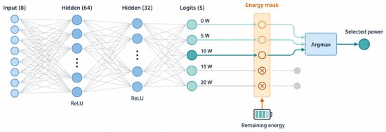
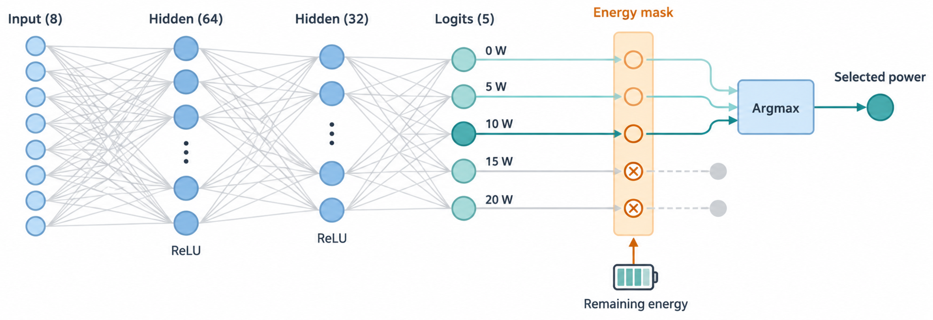
The proposed soft-label policy, denoted SoftMLP, uses a fully connected 8–64–32–5 multilayer perceptron (MLP) with rectified linear unit (ReLU) activation after each hidden layer and 2821 trainable parameters, including biases. The output layer is linear and produces five action logits ${\mathit{o}}_t\in {\mathbb{R}}^5$, corresponding to $\{0,5,10,15,20\}$ W. Figure 2 illustrates the network and subsequent energy-feasible action selection.

Figure 2. MLP architecture and energy-feasible online power selection. The example masks the 15 and 20 W actions and selects 10 W by argmax over the remaining feasible logits; the feasible set changes with the remaining energy.

For this architecture, each forward pass requires $8\times 64+64\times 32+32\times 5=2720$ MACs, 101 bias additions, and 96 ReLU evaluations. Storing all 2821 weights and biases in 32-bit floating-point format requires 11,284 bytes (approximately 11.02 KiB). Separate arrays for the input, both hidden-layer outputs, and the five logits require a further $(8+64+32+5)\times 4=436$ bytes; buffer reuse can reduce this amount. These are static parameter and activation-storage estimates for a direct implementation, excluding program code, stack, normalization constants, and other controller state, rather than measurements of total runtime memory.

Based on the soft target probability $q_t(a\mid b)$, the soft cross-entropy loss is defined as

$$\begin{array}{c}\hfill {\mathcal{L}}_{\mathrm{VA}}\left(\mathit{\varphi }\right)=-{\displaystyle \frac{1}{M_{\mathrm{tr}}}}{\displaystyle \sum _{i=1}^{M_{\mathrm{tr}}}}\sum _{a\in \mathcal{A}\left(b_i\right)}{q}_i\left(a\right)\log p_{\mathit{\varphi }}(a\mid {\mathit{x}}_i),\end{array}$$

(17)

where $M_{\mathrm{tr}}$ is the number of training samples, $\mathit{\varphi }$ is the set of network parameters, $q_i\left(a\right)$ is the supervised soft target probability corresponding to the input sample, and $p_{\mathit{\varphi }}(a\mid {\mathit{x}}_i)$ is the prediction probability of action a by the network.

Table 1 summarizes the network and original hard-/soft-label training settings. Training shuffles the state samples at every epoch and applies the energy-feasible action mask in the cross-entropy loss. Each epoch is followed by full-pass validation rollouts, in which the policy updates its own remaining energy after every action. The selection metric is the mean per-pass relative throughput gap to DP on the validation set, rather than the supervised loss.

Table 1. Network architecture and original distillation training settings.

Item	Setting
Architecture	Fully connected 8–64–32–5; ReLU hidden layers; linear output
Trainable parameters	2821, including biases
Optimizer	Adam; initial learning rate ${10}^{-3}$
Batch size	2048 state samples
Soft-target inverse temperature	$\beta =10$
Stage 1	50 epochs at a fixed learning rate of ${10}^{-3}$
Stage 2	Continue from epoch 50 to at most 150 total epochs
Learning-rate schedule in Stage 2	ReduceLROnPlateau; factor $0.5$, patience 5, absolute improvement threshold $0.001$ percentage points, minimum learning rate ${10}^{-5}$
Early stopping in Stage 2	Stop after 20 consecutive epochs without a new minimum validation mean rollout gap
Checkpoint selection	Lowest validation mean rollout gap across both stages
Training seeds	510001, 510002, 510003; all three retained for evaluation

Stage 2 preserves the learned weights, optimizer state, and random-number state from epoch 50. Its learning-rate scheduler monitors the validation mean rollout gap; with patience 5, the learning rate is halved after six consecutive epochs without an improvement exceeding $0.001$ percentage points relative to the scheduler’s best value. Early stopping instead monitors any strict decrease in the validation gap. The hard-label ablation, denoted HardMLP, uses the same architecture and training protocol as SoftMLP, with one-hot targets in place of DP-derived soft targets. Validation and test data are excluded from gradient updates, and test results are not used for learning-rate adjustment, early stopping, checkpoint selection, or training-seed selection.

4.3. Energy-Feasible Action Masking and Online Decision

Network outputs alone do not guarantee satisfaction of the cumulative energy constraint. We therefore mask actions whose energy costs exceed the remaining budget before selecting an action.

Before action selection, infeasible actions are masked using the current remaining energy $b_t$ as

$$\begin{array}{c}\hfill {\tilde{o}}_{t,a}=\left\{\begin{array}{cc}{o}_{t,a},\hfill & c_a\le b_t,\hfill \\ -\infty ,\hfill & c_a>b_t,\hfill \end{array}\right.\end{array}$$

(18)

where ${\tilde{o}}_{t,a}$ and $o_{t,a}$ are the masked and original logits, respectively, and $c_a$ and $b_t$ are the action cost and remaining budget in discrete energy units.

After masking, actions that exceed the budget have zero probability in $p_{\mathit{\varphi }}(a\mid {\mathit{x}}_t)$. The network selects the feasible action with the highest predicted probability as

$$\begin{array}{c}\hfill a_t^{\mathrm{DNN}}=\arg \underset{a\in \mathcal{A}}{\max }{p}_{\mathit{\varphi }}(a\mid {\mathit{x}}_t),\end{array}$$

(19)

where $a_t^{\mathrm{DNN}}$ is the selected action. Since each selected action satisfies $c_a\le b_t$, the remaining budget stays non-negative throughout the pass. Hence, the total RF energy consumption satisfies ${\sum }_t{P}^{\left(a_t^{\mathrm{DNN}}\right)}\Delta t\le B\Delta E\le E_{\max }$.

The implementation selects the maximum masked logit directly, since softmax preserves the ordering of feasible logits. Thus, online action selection does not require exponentiation or probability normalization. For the five-action set, masking uses five energy-feasibility comparisons, followed by a maximum search and a remaining-energy update.

5. Simulation Setup and Experimental Results

This section evaluates the proposed method using dynamic programming as the discrete-model benchmark and compares it with uniform allocation, elevation heuristic, and greedy baselines. It first presents nominal performance and then tests robustness under strong attenuation, high-orbit, and low-budget conditions, followed by SNR forecast errors and along-track ephemeris errors. The evaluation considers transmission volume, optimality gap, energy-constraint satisfaction, and computational overhead across different decision resolutions. Unless otherwise specified, the simulations use the basic physical parameters listed in Table 2.

Table 2. Basic simulation parameters.

Parameter (Symbol)	Default Value	Parameter (Symbol)	Default Value
Earth Radius ($R_E$)	6371 km	Tx Antenna Gain ($G_t$)	20 dBi
Earth Gravitational Param ($\mu$)	$3.986004418\times {10}^{14}$ ${\mathrm{m}}^3/{\mathrm{s}}^2$	Zenith Atm Attenuation ($A_{\mathrm{zen}}$)	0.4 dB
Orbit Altitude (h)	600 km	Rx Antenna Gain ($G_r$)	35 dBi
Carrier Frequency ($f_c$)	20 GHz	Link Demod Margin ($M_{\mathrm{link}}$)	1 dB
Time Slot Length ($\Delta t$)	5 s	System Noise Temp ($T_{\mathrm{sys}}$)	300 K
Boltzmann Constant (k)	$1.380649\times {10}^{-23}$ $\mathrm{J}/\mathrm{K}$	Ref Tx Power ($P_{\mathrm{ref}}$)	10 W
Min Working Elev (${\theta }_{\min }$)	${10}^{\circ }$	Symbol Rate ($R_s$)	100 Msymbol/s
Fixed Misc Loss ($L_{\mathrm{misc}}$)	2 dB

The default power set is ${\mathcal{P}}_5=\{0,5,10,15,20\}\mathrm{W}$. Table 3 lists the eight MODCODs used for the DVB-S2X-style ACM mapping, their net spectral efficiencies ${\eta }_m$, and ideal $E_s/N_0$ thresholds ${\Gamma }_m^{\mathrm{ideal}}$. Each operating threshold is ${\Gamma }_m={\Gamma }_m^{\mathrm{ideal}}+1$ dB, using the same 1 dB link margin for all modes.

Table 3. MODCOD configurations used in the simulations.

MODCOD	Net Spectral Efficiency (Bit/Symbol)	Ideal ${\mathit{E}}_{\mathit{s}}/{\mathit{N}}_0$ Threshold (dB)
QPSK 2/9	0.434841	$-2.85$
QPSK 9/20	0.889135	0.22
QPSK 11/20	1.088581	1.45
8APSK 5/9-L	1.647211	4.73
8PSK 23/36	1.896173	6.12
16APSK 3/5	2.370043	7.80
32APSK 32/45	3.510192	11.75
64APSK 4/5	4.735354	15.87

The original supervised collection contains 3000 random passes, split at the whole-pass level into 2100 training, 450 validation, and 450 internal test passes (70%/15%/15%). All state samples from a pass remain in the same split. Separately, 3000 additional passes are independently generated from the same scenario distribution for Figure 3a. Their scenario parameter tuples are checked to be non-overlapping with the original collection. This additional evaluation set is not used for training, normalization fitting, or model selection; the models are frozen before its evaluation.

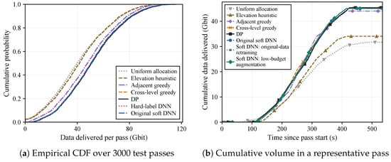
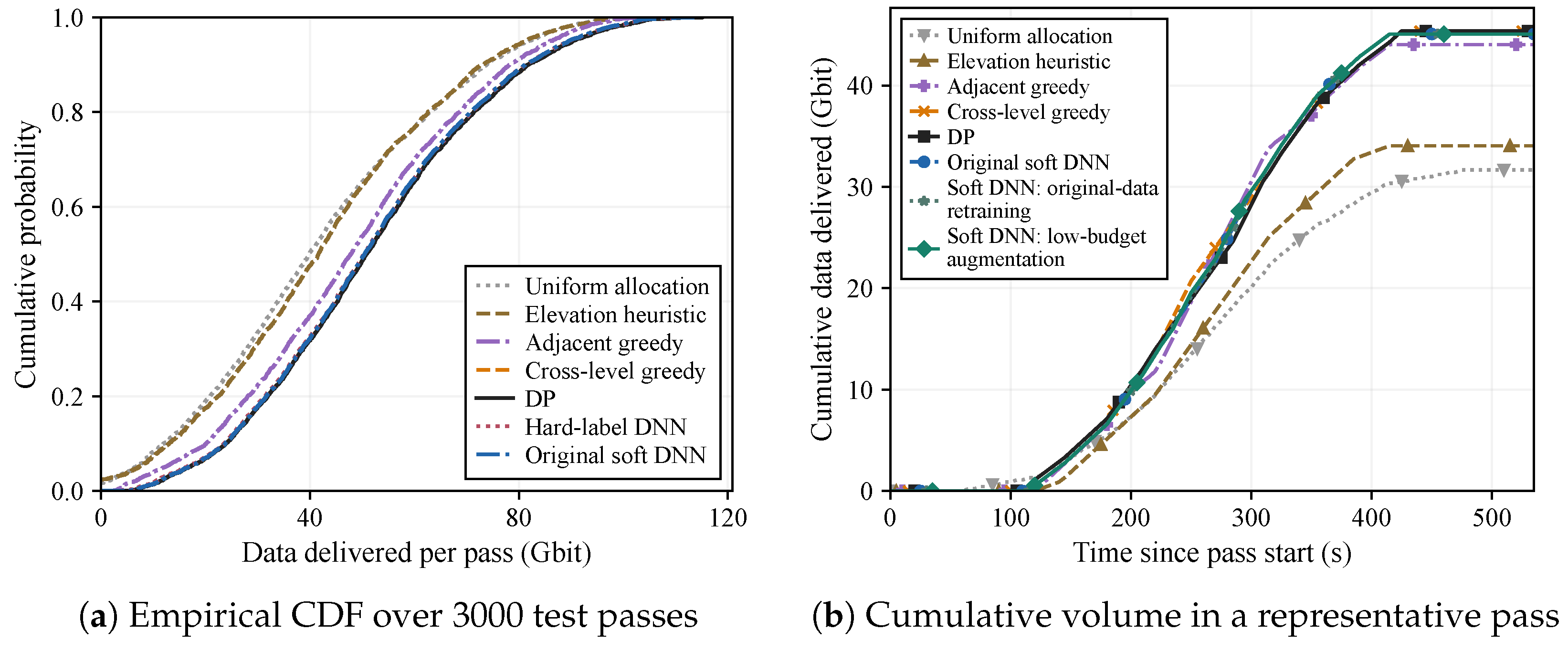
Figure 3. Transmission performance comparison. Panel (a) uses an additional independent set of 3000 test passes.

Formal scenarios sample the orbit altitude $h\sim U(500,800)\mathrm{km}$, maximum elevation ${\theta }_{\max }\sim U({15}^{\circ },{90}^{\circ })$, additional atmospheric attenuation $A_{\mathrm{w}}\sim U(0,6)\mathrm{dB}$, and average power budget $P_{\mathrm{avg}}\sim U(4,16)\mathrm{W}$; the closest-approach angle ${\psi }_0$ is derived from h and ${\theta }_{\max }$ using the geometry in Section 2. Low-budget experiments use $P_{\mathrm{avg}}\sim U(1,4)\mathrm{W}$. For comparison, uniform allocation distributes the energy budget uniformly over feasible slots, while the elevation heuristic assigns fixed weights to low-, medium-, and high-elevation segments. Adjacent-upgrade greedy and offline cross-level greedy allocate energy according to marginal gains over adjacent and arbitrary higher power levels, respectively; both construct a full-pass plan before execution. DP provides the discrete-model optimum. SoftMLP is the proposed soft-label policy, and HardMLP is used only as a supervision ablation. When distinguishing training variants, Original SoftMLP denotes the policy before additional training, Original-data-retrained SoftMLP denotes continuation using only original data, and Mixed-retrained SoftMLP denotes continuation using a mixture of original and additional low-budget data.

Figure 3a provides the empirical Cumulative Distribution Function (CDF) of the actual single-pass transmission volumes for each method on the same additional 3000-pass independent evaluation set described above. For any x-coordinate x, the y-coordinate indicates the proportion of test passes where the method’s transmission volume does not exceed x; thus, for the same cumulative probability, curves further to the right imply higher transmission volumes at corresponding quantiles. DP and traditional methods each correspond to one empirical CDF derived from 3000 passes; for HardMLP and SoftMLP, the curve is the equally weighted average of empirical CDFs from three independent training seeds, not merged into 9000 independent test samples.

To quantify the loss relative to DP, the per-pass optimality gap is defined as $(D_{\mathrm{DP}}-D_{\mathrm{net}})/D_{\mathrm{DP}}\times 100\%$. Averaged over the 3000 test passes and three training seeds, the mean ± sample standard deviation is $0.8849\%\pm 0.0756\%$ for SoftMLP and $1.4611\%\pm 0.1343\%$ for HardMLP. Thus, value-aware soft labels consistently outperform one-hot training under the same architecture and training procedure while retaining 99.115% of DP’s transmission volume on average. Whether this near-optimality can be achieved with lower online inference overhead is examined next.

Figure 3b presents the cumulative transmission volume for a representative pass, characterized by a 653.8 km orbit altitude, $64.1^{\circ }$ maximum elevation, 4.15 dB extra attenuation, 7.30 W average power budget, 107 time slots, and a 535 s duration. Uniform allocation, the elevation heuristic, and adjacent-upgrade greedy achieve approximately 31.66, 34.05, and 44.03 Gbit, respectively, while offline cross-level greedy and DP both reach about 45.37 Gbit. SoftMLP achieves about 45.07 Gbit, only 0.66% below DP, demonstrating that it closely approaches the DP performance benchmark under the same 3900 J energy budget.

Table 4 reports the average single-pass transmission volume for 1000 paired passes under low ($1\sim 4$ W), intermediate ($4\sim 16$ W), and high ($16\sim 20$ W) average power budgets. Original SoftMLP closely approaches DP under the intermediate and high budgets, whereas its gap increases slightly under the low budget. Beyond the difference from the original $4\sim 16$ W training range, low budgets make useful transmission opportunities compete more strongly for limited energy. Because power actions and ACM modes are discrete, a low-power transmission can remain below the decoding threshold, while the energy spent on an ineffective action accounts for a larger fraction of a smaller budget. Accurate joint selection of transmission slots and power levels is therefore especially important, and later decisions have less scope to compensate for earlier allocation errors.

Table 4. Average single-pass transmission volume under different average power budgets.

Method	Low Budget ($1\sim 4$ W)	Intermediate Budget ($4\sim 16$ W)	High Budget ($16\sim 20$ W)
Uniform allocation	11.326	41.633	64.784
Elevation heuristic	16.458	42.525	65.089
Adjacent-upgrade greedy	20.300	48.137	66.029
Offline cross-level greedy	20.897	51.797	68.856
DP	20.903	51.806	68.863
Original SoftMLP	20.388	51.342	68.518

Values are single-pass average transmission volumes in Gbit. Each group contains 1000 paired scenarios; Original SoftMLP results are averages from three training seeds.

Table 5 compares Original SoftMLP with Original-data-retrained SoftMLP and Mixed-retrained SoftMLP. The mixed branch uses 1200 additional low-budget passes (1000 for training and 200 for validation, with no test-set access). In the low-budget group, Mixed-retrained SoftMLP increases the average transmission volume from 20.388 to 20.651 Gbit, reducing the relative gap between mean transmission volumes from 2.46% to about 1.20%. Here, this gap is calculated as $({\overline{D}}_{\mathrm{DP}}-{\overline{D}}_{\mathrm{net}})/{\overline{D}}_{\mathrm{DP}}\times 100\%$, where each overbar denotes the mean over test passes and, for the network, training seeds. Original-data-retrained SoftMLP reaches only 20.404 Gbit, indicating that targeted low-budget augmentation provides benefits beyond additional training updates alone. The trade-off is small: intermediate- and high-budget throughput decreases by only 0.013 and 0.039 Gbit, respectively, with the corresponding relative gaps between mean transmission volumes increasing marginally from 0.90% to 0.92% and from 0.50% to 0.56%. This comparison quantifies the trade-off between improved low-budget performance and the small throughput reductions in the other budget groups.

Table 5. Average single-pass transmission volume of different training schemes across three average power budget groups.

Budget Group	DP	Original SoftMLP	Original-Data-Retrained SoftMLP	Mixed-Retrained SoftMLP
Low Budget ($1\sim 4$ W)	20.903	20.388	20.404	20.651
Intermediate Budget ($4\sim 16$ W)	51.806	51.342	51.345	51.329
High Budget ($16\sim 20$ W)	68.863	68.518	68.511	68.479

Values are single-pass average transmission volumes in Gbit. Each group contains 1000 paired test scenarios; low-budget data was used exclusively for the mixed retraining branch, and network results are equally weighted averages of three seeds.

Low-budget augmentation and retraining protocol. The additional passes target average power budgets of 1–4 W while retaining the original altitude, elevation, and attenuation ranges. DP supervision is generated using the same state-sampling procedure, yielding 497,320 training states and 99,700 validation states. For each of the three original training seeds, both continuation branches start from the same frozen Original SoftMLP checkpoint and use a fresh Adam optimizer with learning rate ${10}^{-4}$, batch size 2048, and 15,000 updates (30 rounds of 500 updates). The original-data branch samples 2048 original states per update; the mixed branch samples 1365 original and 683 low-budget states, with replacement in both cases. Architecture, normalization, soft-target parameter $\beta =10$, and masking remain unchanged. Checkpoint selection includes the starting model and uses only the original 450-pass and additional 200-pass validation sets: the original-range mean rollout gap may increase by at most 0.10 percentage points relative to the starting checkpoint, and the eligible checkpoint minimizing the equal-weight mean gap across the two validation sets is retained. All three seeds are evaluated without test-based selection.

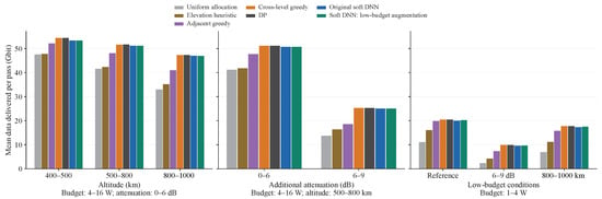
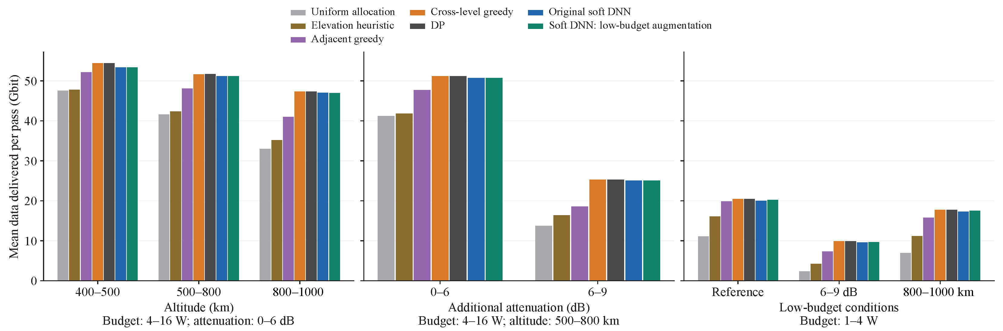
Figure 4 evaluates the adaptability of the network under altitude variation, stronger attenuation, and low-budget constraints. Mixed-retrained SoftMLP maintains relatively stable average gaps across different altitude and attenuation ranges and clearly improves performance in combined low-budget scenarios, indicating good adaptability after targeted retraining. However, it does not guarantee near-optimality in all cases: under combined low-budget and strong-attenuation or high-orbit conditions, performance can still degrade sharply, with worst-case losses approaching complete failure. Thus, the method is robust on average but retains notable tail risk in extreme scenarios.

Figure 4. Actual transmission volume across different altitude, extra attenuation, and low-budget combination scenarios.

To quantify how often large losses occur, Table 6 reports the mean and 95th percentile (P95) of the per-pass relative gap to DP, together with the proportions exceeding 10% and 20%. Each scenario contains 1000 test passes. Nominal and low-budget conditions use average power budgets of 4–16 and 1–4 W, respectively, with altitude 500–800 km and extra attenuation 0–6 dB. The combined cases retain the low budget and change only attenuation to 6–9 dB or altitude to 800–1000 km. The two thresholds describe performance degradation rather than prescribed engineering failure limits.

Table 6. Relative throughput gap to DP and tail risk under different test conditions.

Scenario	Model	Mean Gap (%)	P95 Gap (%)	Gap $>10\%$ (% of Passes)	Gap $>20\%$ (% of Passes)
Nominal	Original	0.90	2.02	0.27	0.07
	Mixed	0.93	2.14	0.30	0.10
Low budget	Original	2.96	10.80	5.83	1.23
	Mixed	1.35	3.88	0.80	0.27
Low budget + strong attenuation	Original	4.99	18.28	10.95	3.67
	Mixed	2.55	10.41	5.58	1.94
Low budget + high altitude	Original	3.72	12.88	6.52	2.49
	Mixed	1.87	5.91	2.82	1.44

Original and Mixed abbreviate Original SoftMLP and Mixed-retrained SoftMLP, respectively. Each metric is computed separately for each of three training seeds and then equally averaged, including P95. Relative-gap metrics exclude DP-zero passes: 0, 0, 38, and 8 of 1000 in the four scenarios, respectively, leaving 1000, 1000, 962, and 992 valid passes. Nominal and low-budget rows use the existing budget-test sets; combined rows use the separate combined-condition tests.

Mixed retraining reduces the proportion of low-budget passes with gaps above 10% from 5.83% to 0.80%, while nominal tail metrics increase slightly. Under combined low-budget and strong-attenuation conditions, the proportion decreases from 10.95% to 5.58%, but 1.94% of valid passes still exceed a 20% gap. Thus, targeted retraining reduces tail risk without eliminating large losses under adverse conditions. The mean gap here averages per-pass relative losses; it differs from the relative difference between mean throughputs used in the preceding budget discussion.

The largest tail metrics in Table 6 occur under low budgets combined with strong attenuation. In this regime, a nonzero power action can remain below the ACM decoding threshold, consuming energy without transmitting data and reducing the budget available for later slots. In one saved tail case (seed 510001; altitude 679.3 km, extra attenuation 7.84 dB, and budget 775 J), Original SoftMLP spends 300 J on zero-return actions before DP begins transmitting and delivers 0.435 Gbit, compared with 1.522 Gbit for DP and 1.305 Gbit for Mixed-retrained SoftMLP. This case illustrates the sensitivity to power selection near ACM thresholds. Action masking adds no restriction beyond the physical energy-feasibility condition at a given state, although earlier allocation errors can restrict later choices. With the architecture and masking rules unchanged, the reduction in tail losses after mixed retraining shows that targeted training improves low-budget adaptation, without attributing all tail losses to a single cause.

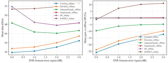
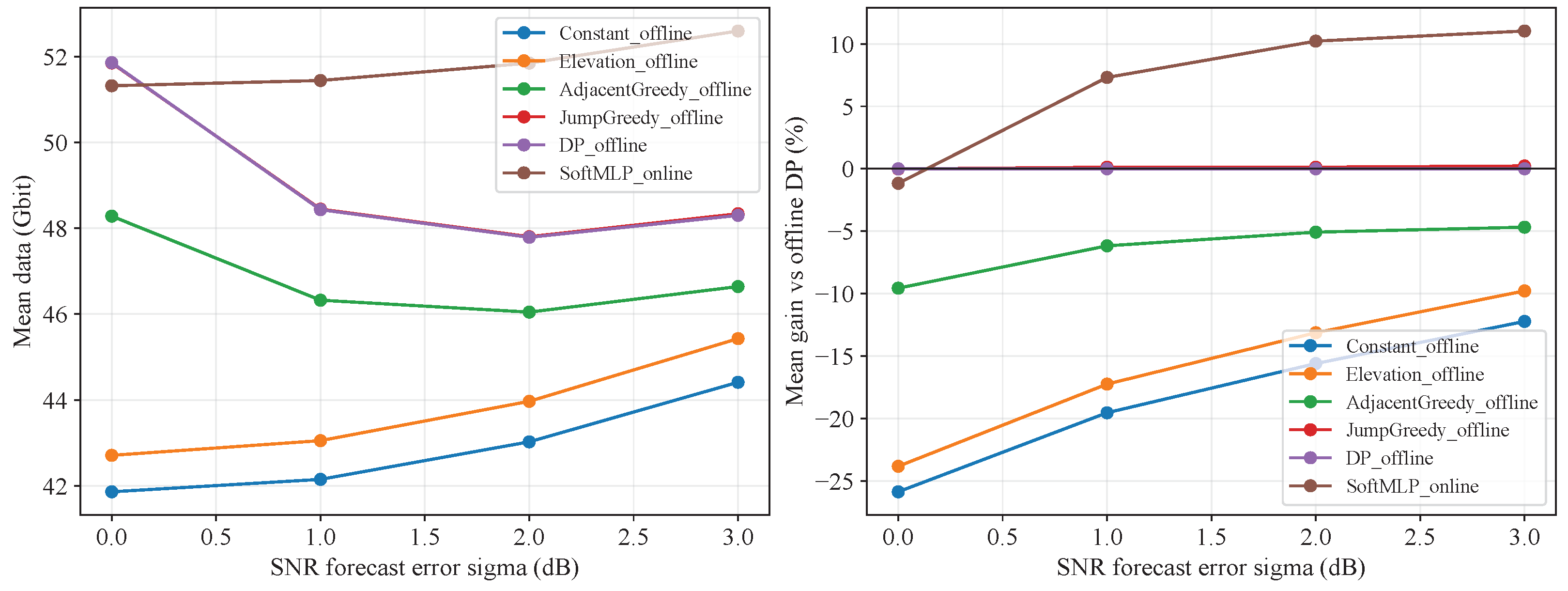
The previous experiments assumed perfect forecasts. To assess online decision-making under forecast uncertainty, two groups of paired tests are constructed. The first introduces slotwise SNR forecast errors with standard deviations of 0, 1, 2, and 3 dB; true reference SNRs are generated by adding zero-mean Gaussian errors to the forecasts before ACM mapping. Uniform allocation, the elevation heuristic, adjacent-upgrade greedy, offline cross-level greedy, and forecast-based offline DP construct one-shot plans using only predicted per-slot throughput, whereas Original SoftMLP uses the observed SNRs and updates the remaining energy slot by slot. Forecast-based offline DP denotes the DP plan obtained from the predicted channel; it is distinct from the realized-channel DP benchmark used for retrospective gap evaluation in the later online-baseline comparisons. All methods are evaluated against the same actual per-slot throughput tables.

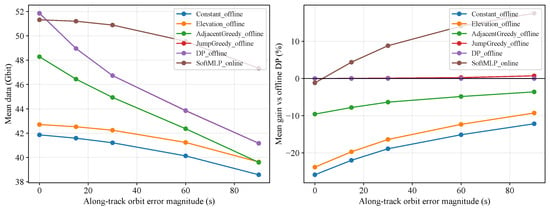
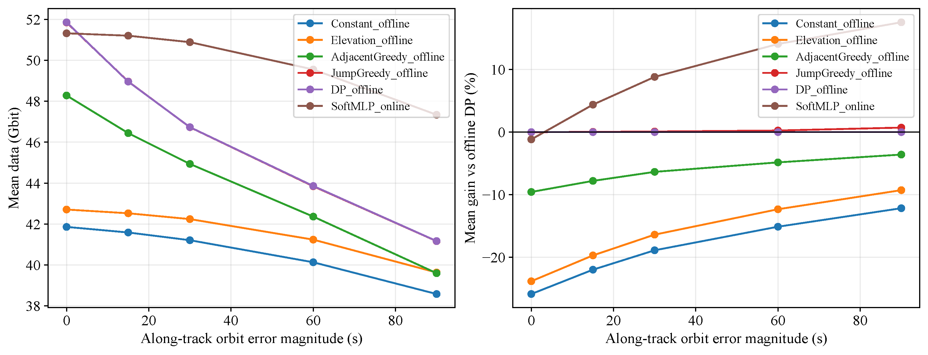
Figure 5 and Figure 6 examine the advantage of online energy reallocation under imperfect forecasts. For SNR forecast errors of 0–3 dB, SoftMLP remains close to forecast-based offline DP under nominal conditions and increasingly outperforms that fixed plan as the forecast deteriorates, confirming that real-time SNR feedback reduces action mismatch. In the along-track ephemeris-error test, time offsets of up to 90 s represent leading or lagging positions along the nominal orbit. These offsets cause offline plans to become misaligned with the actual pass geometry, whereas SoftMLP uses the observed elevation and SNR to reallocate energy dynamically; it achieves a clear gain over forecast-based offline DP and achieves higher throughput in most of the 900 leading/lagging trials. Together, these results show that online state feedback supports adaptation to both channel and geometry forecast errors in the tested scenarios.

Figure 5. Actual transmission volume and its gain relative to forecast-based offline DP under SNR forecast errors.

Figure 6. Actual transmission volume and its gain relative to forecast-based offline DP under along-track ephemeris errors represented by time offsets.

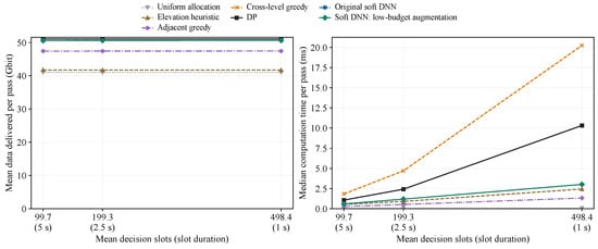
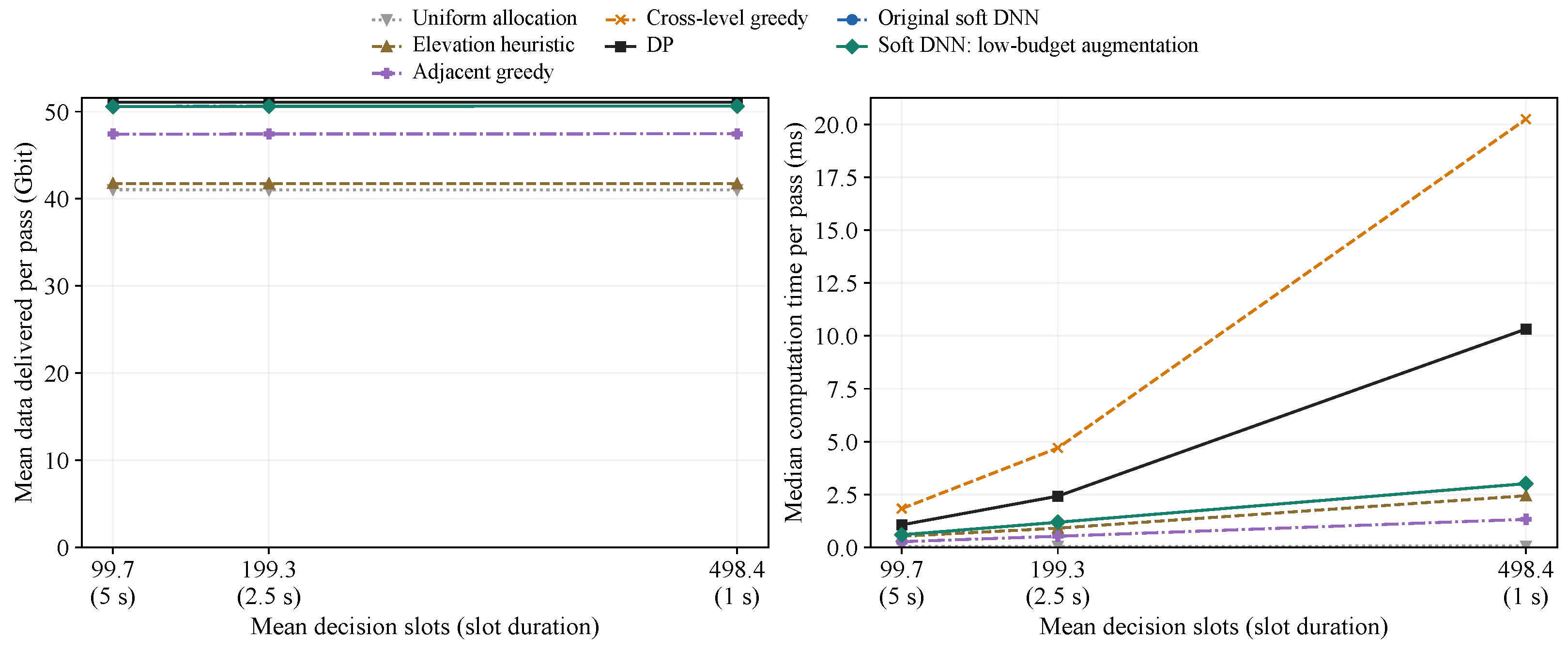
Figure 7 examines the effect of decision resolution on performance and computational cost. Refining the slot length from 5 s to 2.5 s and 1 s increases the number of decisions but keeps the mean per-pass relative gap to DP of Mixed-retrained SoftMLP near 0.93–1.03%, showing no meaningful performance loss. At the 1 s resolution, the network remains close to DP while running about 3.42× faster than the DP implementation and 6.71× faster than offline cross-level greedy. The timing includes network inference, remaining-energy updates, and action masking over the full pass while excluding geometry/link preprocessing, model loading, and disk I/O.

Figure 7. Actual transmission volume and computation time under different decision resolutions (Each timed DP call performs one full-pass solve, including backward recursion and policy recovery. Network timing covers all slots, including inference, action masking, and energy updates. Geometry/link and feature preprocessing, model loading, and disk I/O are excluded).

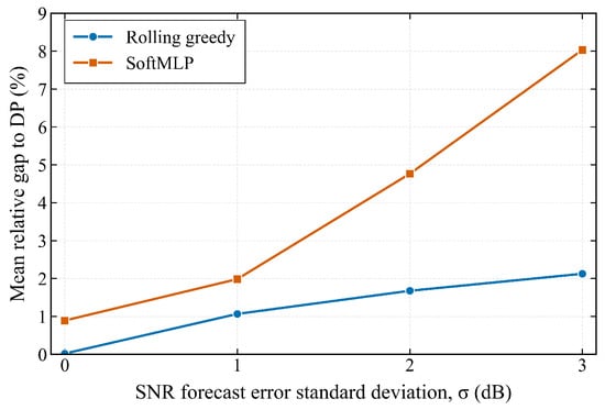
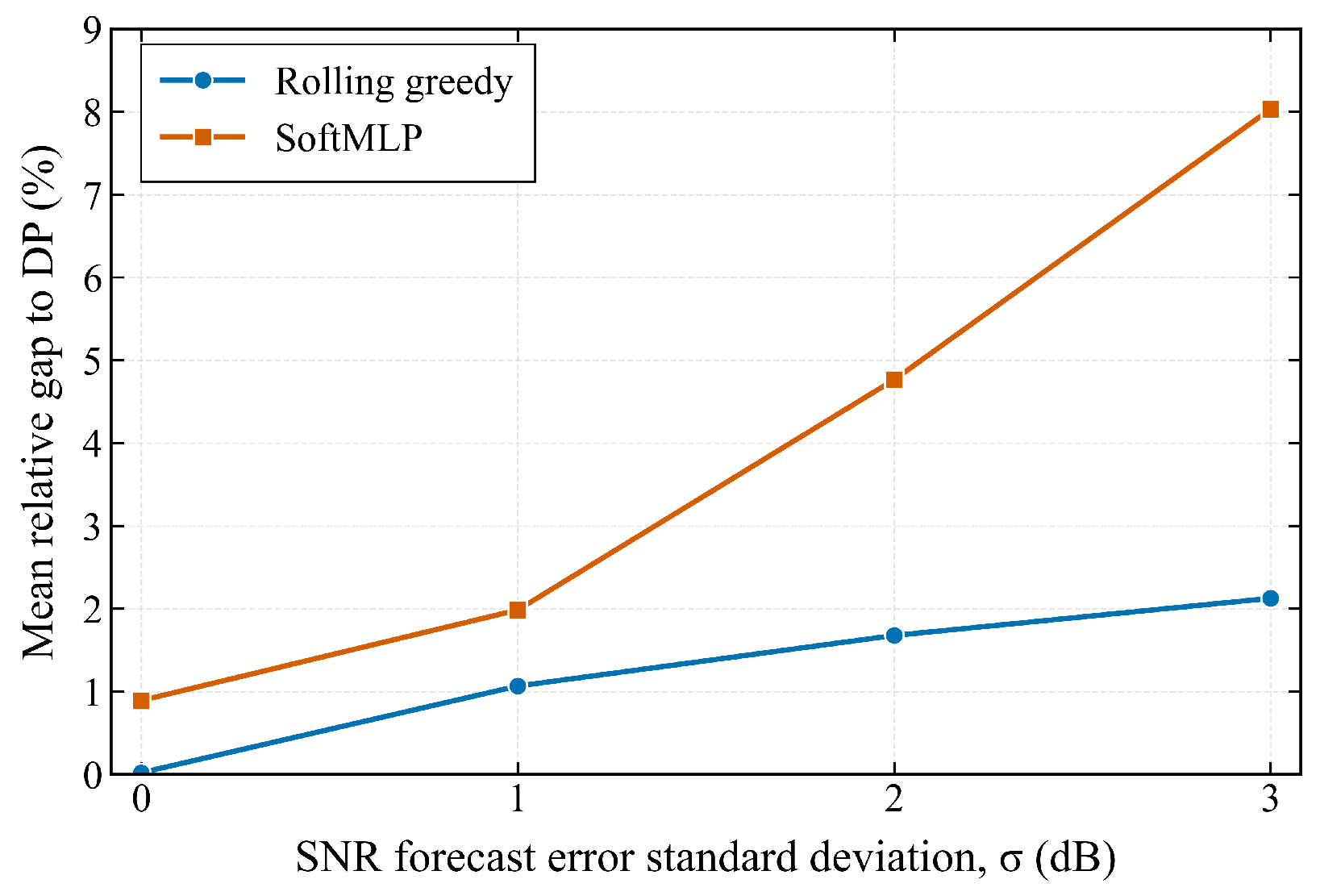
To distinguish the benefit of online adaptation from that of the learned policy, Figure 8 compares Original SoftMLP with rolling cross-level greedy. At each slot, this baseline replaces the current row of the predicted reward table with rewards computed from the observed SNR while retaining the nominal predictions for future slots. Starting from zero-power assignments over the remaining horizon, cross-level greedy repeatedly selects the affordable upgrade with the largest positive reward gain per unit of additional energy, allowing direct jumps across power levels. It executes only the first action of the resulting plan, subtracts its energy cost from the actual remaining budget, and repeats the planning procedure at the next slot. Future realized SNRs are never used in this process.

Figure 8. Rolling cross-level greedy and SoftMLP under SNR forecast errors.

The comparison uses 1000 newly generated test passes from the nominal scenario distribution, separate from the earlier test sets and shared with the subsequent Double DQN comparison. Both methods use exactly the same pass geometries, realized SNR perturbations, 5 s slots, power levels, initial energy budgets, and actual throughput evaluation. Both observe the current realized SNR and geometry and update their own remaining energy after every action. Rolling cross-level greedy additionally processes the remaining nominal reward forecast derived from the known model, whereas SoftMLP retains its original eight-dimensional state without explicitly reading that table. Thus, the comparison controls the physical conditions, online observations, action space, and energy constraint while preserving each method’s decision mechanism. SoftMLP uses three frozen training seeds without retraining or test-based model selection. Its per-pass gaps are equally averaged over the seeds and then over the test passes. For both methods, the realized-channel DP benchmark is recomputed on the full realized channel trajectory only for retrospective evaluation.

Rolling cross-level greedy achieves a lower mean per-pass relative gap to the realized-channel DP benchmark throughout the tested forecast-error range in Figure 8. At $\sigma =0$ dB, the gaps are 0.02% for rolling cross-level greedy and 0.89% for SoftMLP; at $\sigma =3$ dB, they are 2.13% and 8.04%, respectively. These results show that the benefit of adapting online over one-shot planning is not exclusive to the neural policy. Repeated replanning using the remaining nominal forecast provides better transmission performance in these tests. Our objective, however, is to retain useful transmission performance with a small online computational workload, leaving processing capacity available for other onboard tasks.

Table 7 quantifies this trade-off using measured cumulative CPU time per complete pass (Rolling cross-level greedy combines repeated candidate search, comparisons, divisions, and data updates, whereas SoftMLP is dominated by fixed-size matrix multiply–accumulate operations. Floating-point operation (FLOP) or MAC counts alone do not fully capture these different execution patterns. We therefore use cumulative CPU time under the same conditions to compare processor occupation). The timing uses the same prespecified subset of 40 test passes for both methods, on a single CPU thread in Windows 11 with Python 3.13.5 and NumPy 2.1.3 (Intel CPU Family 6, Model 197, Stepping 2). After warm-up, inputs are preloaded, and inference or replanning is repeated in three timed blocks per model and error level, each lasting at least 0.5 s to amortize the Windows CPU timer granularity. Total process CPU time is divided by the number of complete passes executed, and the resulting times are averaged over blocks and, for SoftMLP, equally over its three seeds. Both timings include decision computation and remaining-energy updates; rolling cross-level greedy also includes copying the remaining forecast table. Sensing, geometry/link and ACM preprocessing, feature construction, model loading, and disk I/O are excluded for both methods.

Table 7. Cumulative CPU time of rolling cross-level greedy and SoftMLP.

SNR Error Standard Deviation (dB)	Rolling Cross-Level Greedy (ms/pass)	SoftMLP (ms/pass)	CPU Time Reduction (%)
0	83.724	0.554	99.34
1	83.594	0.560	99.33
2	83.203	0.560	99.33
3	83.464	0.565	99.32

Values are mean cumulative process CPU times per complete pass over the same 40 paired test passes. SoftMLP equally averages three frozen seeds. Reduction is relative to rolling cross-level greedy and is calculated from unrounded measurements.

The measured mean cumulative CPU time is approximately 83–84 ms per pass for rolling cross-level greedy and 0.55–0.56 ms for SoftMLP, a reduction of approximately 99.3% in the tested implementations. SoftMLP therefore trades some transmission performance for substantially lower online processor occupation. The performance loss increases with forecast uncertainty and is explicitly retained in this comparison. These timings characterize the tested implementations on the general-purpose CPU. The measured acceleration is specific to this platform and these implementations; its magnitude may change with the target processor and implementation. No embedded or hardware-in-the-loop validation has been performed. The operation and storage counts above describe the policy’s static resource requirements but do not establish execution time, electrical-energy consumption, or end-to-end deployment viability on an onboard processor.

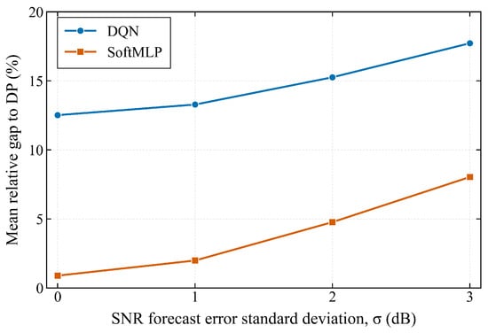
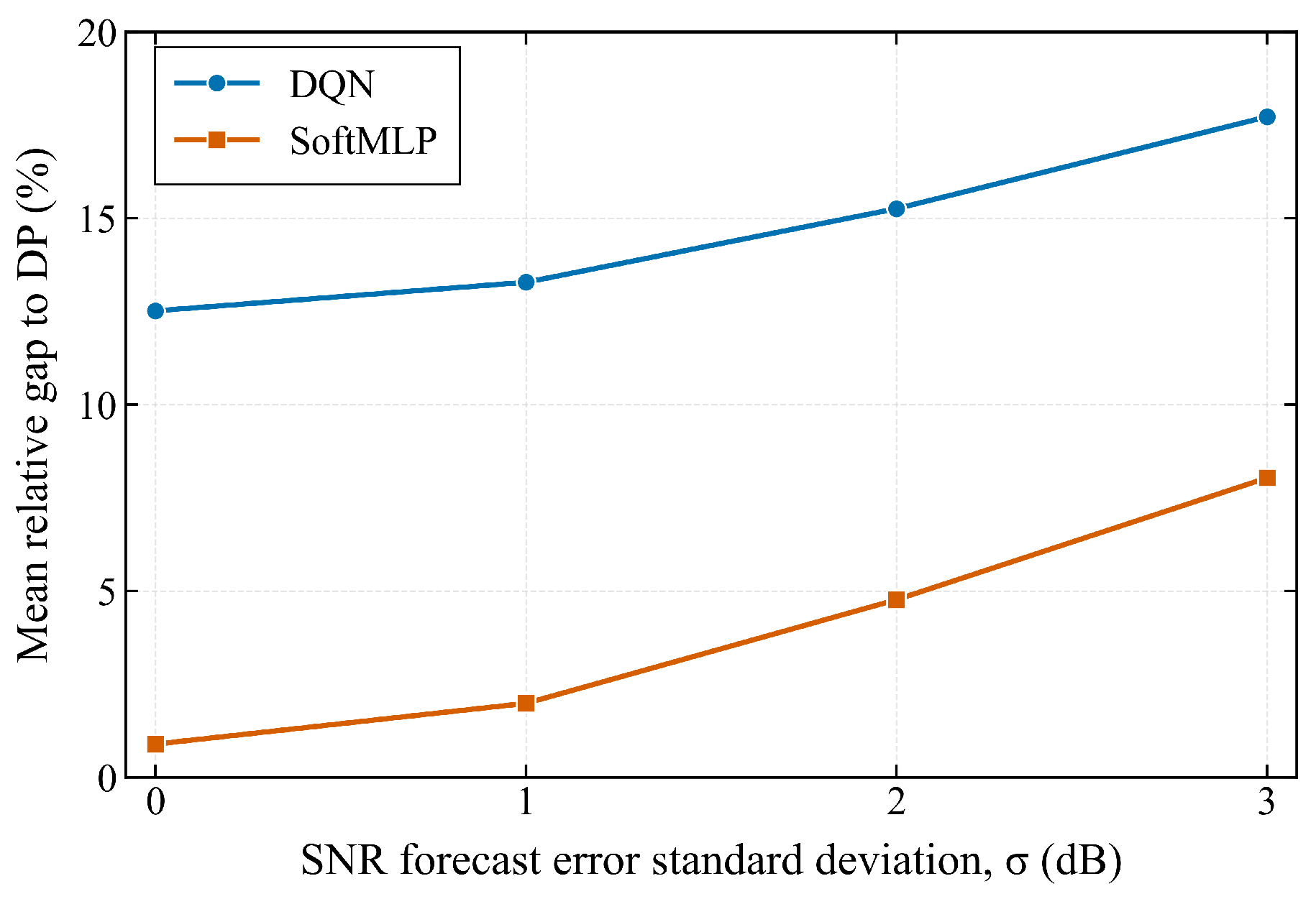
Finally, Figure 9 compares Original SoftMLP with a Double DQN baseline using five-step returns and energy-feasible action masking. Both methods use an 8–64–32–5 MLP with 2821 parameters, the same eight-dimensional online state, power actions, and cumulative energy constraint. Double DQN learns from transmitted-data rewards without DP labels, whereas SoftMLP uses the DP-derived soft targets. The Double DQN learning rate and return length are selected on the original 450-pass validation set; each retained training seed receives eight million interaction steps, and its checkpoint is selected by the validation rollout gap. All models are frozen before evaluation on the same 1000 test passes used in Figure 8. Both policies observe the current realized SNR and geometry without access to future realized SNRs. The curves equally average three training seeds, with each seed’s gap averaged over the paired test passes relative to DP recomputed on the full realized channel trajectory.

Figure 9. Equal-capacity Double DQN and SoftMLP under SNR forecast errors.

SoftMLP has a lower mean gap throughout the tested SNR forecast-error range. At $\sigma =0$ dB, its gap is 0.89%, compared with 12.52% for Double DQN; at $\sigma =3$ dB, the gaps increase to 8.04% and 17.72%, respectively. These results support the effectiveness of DP-guided distillation at the evaluated network capacity and training budget. The advantage may benefit from the teacher’s action-value information, which provides richer supervision than interaction rewards alone. The conclusion is limited to the tested architecture, training settings, scenario distribution, and forecast-error model.

Taken together, Figure 3, Figure 4, Figure 5, Figure 6, Figure 7, Figure 8 and Figure 9 show that value-aware distillation improves over hard-label imitation, achieves near-DP average performance under nominal conditions, and reduces computation relative to the tested DP and offline cross-level greedy implementations at finer decision resolutions. The rolling cross-level greedy comparison and Table 7 further demonstrate a performance–computation trade-off: SoftMLP incurs a larger transmission gap but occupies substantially less CPU time. The equal-capacity Double DQN comparison supports using DP action-value supervision within the evaluated setting. Tail failures under combined low-budget and adverse-link conditions remain an important limitation.

6. Conclusions

This paper proposes a compact DP-distilled policy for power allocation during energy-constrained LEO satellite passes. Soft action-value targets retain information about the relative quality of power actions, while energy-feasible action masking enforces the cumulative energy constraint. The policy achieves near-DP average transmission performance under nominal test conditions and adapts to observed channel and geometry changes. Rolling cross-level greedy performs better in the online comparison, but SoftMLP occupies substantially less cumulative CPU time in the tested implementations. The contribution is therefore a performance–computation trade-off: offline teacher computation and training enable inexpensive online decisions, potentially preserving shared processing capacity for other onboard tasks. Transmission losses under forecast uncertainty and tail failures in adverse scenarios remain limitations. Future work will evaluate deployment-level resource savings on target hardware.

References

- Su, Y.; Liu, Y.; Zhou, Y.; Yuan, J.; Cao, H.; Shi, J. Broadband LEO Satellite Communications: Architectures and Key Technologies. IEEE Wirel. Commun. 2019, 26, 55–61. [Google Scholar] [CrossRef] [Scilit]
- Di, B.; Song, L.; Li, Y.; Poor, H.V. Ultra-Dense LEO: Integration of Satellite Access Networks into 5G and Beyond. IEEE Wirel. Commun. 2019, 26, 62–69. [Google Scholar] [CrossRef] [Scilit]
- Kodheli, O.; Lagunas, E.; Maturo, N.; Sharma, S.K.; Shankar, B.; Montoya, J.F.M.; Duncan, J.C.M.; Spano, D.; Chatzinotas, S.; Kisseleff, S.; et al. Satellite Communications in the New Space Era: A Survey and Future Challenges. IEEE Commun. Surv. Tutor. 2021, 23, 70–109. [Google Scholar] [CrossRef] [Scilit]
- Centenaro, M.; Costa, C.E.; Granelli, F.; Sacchi, C.; Vangelista, L. A Survey on Technologies, Standards and Open Challenges in Satellite IoT. IEEE Commun. Surv. Tutor. 2021, 23, 1693–1720. [Google Scholar] [CrossRef] [Scilit]
- Di, B.; Zhang, H.; Song, L.; Li, Y.; Li, G.Y. Ultra-Dense LEO: Integrating Terrestrial-Satellite Networks Into 5G and Beyond for Data Offloading. IEEE Trans. Wirel. Commun. 2019, 18, 47–62. [Google Scholar] [CrossRef] [Scilit]
- Lin, Z.; Niu, H.; An, K.; Wang, Y.; Zheng, G.; Chatzinotas, S.; Hu, Y. Refracting RIS-Aided Hybrid Satellite-Terrestrial Relay Networks: Joint Beamforming Design and Optimization. IEEE Trans. Aerosp. Electron. Syst. 2022, 58, 3717–3724. [Google Scholar] [CrossRef] [Scilit]
- Morello, A.; Mignone, V. DVB-S2X: The New Extensions to the Second Generation DVB Satellite Standard DVB-S2. Int. J. Satell. Commun. Netw. 2016, 34, 323–325. [Google Scholar] [CrossRef] [Scilit]
- Zhang, P.; Wang, X.; Ma, Z.; Liu, S.; Song, J. An Online Power Allocation Algorithm Based on Deep Reinforcement Learning in Multibeam Satellite Systems. Int. J. Satell. Commun. Netw. 2020, 38, 450–461. [Google Scholar] [CrossRef] [Scilit]
- Zeng, G.; Zhan, Y.; Xie, H.; Jiang, C. Resource Allocation for Networked Telemetry System of Mega LEO Satellite Constellations. IEEE Trans. Commun. 2022, 70, 8215–8228. [Google Scholar] [CrossRef] [Scilit]
- Xu, J.; Fan, S.; Zhao, Z.; Li, F.; Zhang, Y. A Novel Deep Reinforcement Learning Architecture for Dynamic Power and Bandwidth Allocation in Multibeam Satellites. Acta Astronaut. 2023, 204, 73–82. [Google Scholar] [CrossRef] [Scilit]
- Sun, H.; Chen, X.; Shi, Q.; Hong, M.; Fu, X.; Sidiropoulos, N.D. Learning to Optimize: Training Deep Neural Networks for Wireless Resource Management. In Proceedings of the 2017 IEEE 18th International Workshop on Signal Processing Advances in Wireless Communications (SPAWC), Sapporo, Japan, 3–6 July 2017; pp. 1–6. [Google Scholar] [CrossRef] [Scilit]
- Liu, S.; Hu, X.; Wang, W. Deep Reinforcement Learning Based Dynamic Channel Allocation Algorithm in Multibeam Satellite Systems. IEEE Access 2018, 6, 15733–15742. [Google Scholar] [CrossRef] [Scilit]
- Liao, X.; Hu, X.; Liu, Z.; Ma, S.; Xu, L.; Li, X.; Wang, W.; Ghannouchi, F.M. Distributed Intelligence: A Verification for Multi-Agent DRL-Based Multibeam Satellite Resource Allocation. IEEE Commun. Lett. 2020, 24, 2785–2789. [Google Scholar] [CrossRef] [Scilit]
- Lin, Z.; Ni, Z.; Kuang, L.; Jiang, C.; Huang, Z. Dynamic Beam Pattern and Bandwidth Allocation Based on Multi-Agent Deep Reinforcement Learning for Beam Hopping Satellite Systems. IEEE Trans. Veh. Technol. 2022, 71, 3917–3930. [Google Scholar] [CrossRef] [Scilit]
- Huang, J.; Yang, Y.; Lee, J.; He, D.; Li, Y. Deep Reinforcement Learning-Based Resource Allocation for RSMA in LEO Satellite-Terrestrial Networks. IEEE Trans. Commun. 2024, 72, 1341–1354. [Google Scholar] [CrossRef] [Scilit]
- Nasir, Y.S.; Guo, D. Multi-Agent Deep Reinforcement Learning for Dynamic Power Allocation in Wireless Networks. IEEE J. Sel. Areas Commun. 2019, 37, 2239–2250. [Google Scholar] [CrossRef] [Scilit]
- Kourogiorgas, C.I.; Panagopoulos, A.D. A Rain-Attenuation Stochastic Dynamic Model for LEO Satellite Systems Above 10 GHz. IEEE Trans. Veh. Technol. 2015, 64, 829–834. [Google Scholar] [CrossRef] [Scilit]
- de Sombre, W.; Asadi, A.; Bhattacherjee, D.; Vasisht, D.; Ortiz, A. SkyLink: Scalable and Resilient Link Management in LEO Satellite Networks. IEEE Trans. Commun. 2026, 74, 1421–1434. [Google Scholar] [CrossRef] [Scilit]
Disclaimer/Publisher’s Note: The statements, opinions and data contained in all publications are solely those of the individual author(s) and contributor(s) and not of MDPI and/or the editor(s). MDPI and/or the editor(s) disclaim responsibility for any injury to people or property resulting from any ideas, methods, instructions or products referred to in the content. |
© 2026 by the authors. Licensee MDPI, Basel, Switzerland. This article is an open access article distributed under the terms and conditions of the Creative Commons Attribution (CC BY) license.