


Abstract
Sixth-generation (6G) networks will serve large pre-trained artificial intelligence (AI) foundation models from cloud, edge and device tiers, but placing, compressing and scheduling them under latency, energy and accuracy constraints remains open. This paper proposes Massive AI Model Orchestration (MAIMO), a three-tier framework that manages model residency and request routing inside the radio access and core networks. The orchestration problem is formulated as a mixed-integer multi-objective program for which a Pareto-optimal solution is proved to exist and whose offline placement-routing version is shown to be NP-hard. An online controller couples a bidirectional long short-term memory (BiLSTM) traffic predictor with proximal policy optimization (PPO). The evaluation is simulation-only, in a purpose-built system-level simulator calibrated to standardized urban-macrocell channel models. Over 20 paired replications, MAIMO halves the mean end-to-end latency of cloud-only service (11.3 ms against 22.7 ms), serves ultra-reliable low-latency vehicle-to-everything requests in 2.1 ms on average with warm caches and attains the lowest service-level-agreement violation rate among schemes meeting the accuracy floor, while tying deep Q-network and contextual-bandit controllers on mean latency. A transparent analytic energy model gives 5.46 J per inference against 16.73 J for cloud-only service, and constrained carbon-aware workload shifting reduces operational carbon by 27.2%.
1. Introduction
1.1. Motivation and Context
The transition from fifth-generation (5G) to sixth-generation (6G) networks is a re-architecting of wireless networks around native intelligence rather than an incremental capacity upgrade. The IMT-2030 framework of the International Telecommunication Union Radiocommunication Sector (ITU-R) places connection density in the range 106–108 devices per km2 and gives, as illustrative capability values, peak data rates of 50, 100 and 200 Gbit/s and user-experienced data rates of 300 and 500 Mbit/s [1]. Meeting these targets under realistic energy and spectrum constraints requires artificial intelligence (AI) inference to be embedded in the network fabric, from the physical (PHY) layer up to the application plane. Foundation models, large pre-trained networks that can be fine-tuned for diverse downstream tasks, let operators maintain a compact set of general-purpose models and adapt them on demand instead of training a task-specific model for each network function [2,3].
Unlike large language models (LLMs) such as GPT-4 [4], which are optimized for autoregressive text generation, the foundation models considered here are large pre-trained architectures, including transformers [5] and masked autoencoders [6], that generalize zero-shot or few-shot to wireless tasks such as channel estimation, semantic compression and resource allocation. PHY-layer foundation models process complex-valued signal tensors rather than token sequences and face sub-millisecond latency budgets and strict memory limits on edge hardware.
The central challenge addressed here is not training these models but orchestrating their deployment across heterogeneous infrastructure in real time. A single 6G base station may simultaneously serve vehicles requiring 2 ms ultra-reliable low-latency communication (URLLC), extended-reality headsets demanding 10 Gbit/s at 5 ms application latency, and industrial Internet of Things (IoT) sensors that tolerate 50 ms but require 99.99% packet delivery [7,8]. No single model size or placement serves all three. Massive AI Model Orchestration (MAIMO) therefore maintains a portfolio of model variants at different tiers and routes each inference request to the tier that minimizes a weighted combination of latency, energy and accuracy penalty.
1.2. Related Work
Research on AI for networks spans four overlapping threads. At the PHY layer, O’Shea and Hoydis [9] showed that end-to-end autoencoder training can match or exceed conventional signal processing on constrained channels; the idea has been extended to goal-oriented semantic communication [10], attention-based channel estimation [11], deep-learning downlink channel prediction in frequency-division duplex (FDD) massive multiple-input multiple-output (MIMO) systems [12] and learning-to-optimize resource allocation [13].
Deploying large models at the edge requires aggressive compression. Low-Rank Adaptation (LoRA) [14] reduces the number of trainable fine-tuning parameters by up to 10,000× while performing on par with or better than full fine-tuning on the benchmarks evaluated; BranchyNet [15] exits inference at the shallowest sufficient layer; DistilBERT-style distillation [16] yields students with about 40% fewer parameters that run about 60% faster and retain about 97% of the teacher’s performance; sparse convolutions [17] skip computation at inactive sites; and FlashAttention [18] reduces attention memory from O(N2) to O(N) through IO-aware tiling.
Federated learning (FL) [19] aggregates model updates from distributed devices without centralizing raw data, but in wireless settings it must cope with non-independent and identically distributed (non-IID) data across cells, unreliable uplinks and heterogeneous device budgets. Gradient compression [20] and differential privacy [21,22] are standard augmentations that trade model quality for bandwidth or privacy, and Model-Agnostic Meta-Learning (MAML) [23] provides fast few-shot adaptation from a shared initialization.
For AI-native 6G, Letaief et al. set out a roadmap [24] and the enabling technologies of edge intelligence [25]; the Open Radio Access Network (O-RAN) Alliance [26,27] and the European Telecommunications Standards Institute (ETSI) Experiential Networked Intelligence (ENI) group [28] define open interfaces for AI-driven radio access network (RAN) management; and the 3rd Generation Partnership Project (3GPP) TR 38.843 [29] documents the Release-18 study on AI and machine learning (ML) for the New Radio (NR) air interface. These efforts still treat AI as a plug-in to existing architectures rather than as a network element with its own resources, lifecycle and energy management.
The existing work addresses either a single tier (edge-focused surveys [25] or cloud-scale model-parallel training [30]) or a single model type (language models [3], vision transformers [31]). To the best of our knowledge, none jointly optimize latency, energy and model accuracy across three heterogeneous tiers under time-varying 6G traffic, which is the gap this work addresses.
1.3. Contributions
This paper makes four contributions. First, it proposes MAIMO, a three-tier framework that manages model selection, placement, compression and request routing across cloud, edge and device tiers, and evaluates its implemented components end to end in a purpose-built system-level simulator; federated fine-tuning, split inference, on-device personalization and O-RAN signaling are specified as architectural design elements for extension and are not evaluated (Section 1.4). Second, it states the orchestration problem as a mixed-integer multi-objective program, proves that a Pareto-optimal solution exists (Theorem 1) and shows that the offline placement-routing problem is NP-hard (Remark 4). Third, it designs a controller that couples a bidirectional long short-term memory (BiLSTM) traffic predictor with a deep reinforcement learning (DRL) agent trained by proximal policy optimization (PPO). Over 20 paired replications, the controller halves the mean end-to-end latency of the cloud-only baseline (11.34 ms against 22.72 ms) and attains the lowest service-level agreement (SLA) violation rate among the schemes that meet the task-success floor, although its mean latency is statistically tied with those of a deep Q-network (DQN) and a linear upper-confidence-bound (LinUCB) contextual-bandit controller (Section 6.3). Fourth, it provides a transparent, hand-checkable analytic energy-accounting method, 5.46 J per inference at the nominal tier split against 16.73 J for cloud-only service, with a sensitivity analysis under which the energy reduction against cloud-only stays within 57.3–71.1% (95% interval, all inputs varied jointly), and a carbon analysis whose constrained result is a 27.2% reduction (0.425 to 0.310 g CO2e per 1000 inferences).
The rest of the paper is organized as follows. Section 2 presents the system model, the multi-objective formulation and the learning-theoretic status of the controller; Section 3 and Section 4 describe the architecture and the orchestration framework; Section 5 sets out the simulation methodology, including the verification and validation of the simulator; Section 6 reports the results, including mobility, priority-scheduling and overhead studies; Section 7 analyzes energy and carbon; Section 8 discusses open challenges, including physical-layer security and digital twins; and Section 9 concludes.
1.4. Scope of the Evaluation
MAIMO is evaluated only in a purpose-built, discrete-time, system-level simulator: no component was deployed on a testbed, an operator network or physical accelerators, and no over-the-air transmission, power measurement or live traffic trace contributed to any reported number. Table 1 gives the status of every component and the sections that describe it and, where applicable, reports their results. Implemented in simulation denotes an executable code that is exercised on every simulated request and contributes to the latency, task-success, SLA and cache statistics. Modeled analytically denotes a closed-form relation parameterized from datasheets, published measurements or stated assumptions; its outputs, including all energy and carbon figures, are model estimates rather than experimental results. Conceptual (not evaluated) denotes an architectural design element that defines an interface for extension and contributes no quantitative result. Such elements are not simulated because each would require model-level training with real weights and data, or a running O-RAN software stack, which was not implemented or used in this study and whose behavior a system-level simulator could only assume, not validate. Split inference would let a device or edge node run the first layers of a large model and upload intermediate features instead of raw data; federated fine-tuning and on-device personalization would adapt edge and device variants to local data without moving that data; O-RAN integration would host the controller as an application of the near-real-time RAN Intelligent Controller (RIC), exchanging reports and control commands with RAN nodes over an extended E2 interface; the non-terrestrial and terahertz extensions would carry the framework to satellite, aerial and sub-terahertz links; and embodied-carbon accounting would add the manufacturing footprint of the hardware to its operational carbon.
Table 1.
Scope of the evaluation: status and evidence basis of each MAIMO component.
2. Theoretical Foundations of MAIMO
2.1. System Model and Notation
Let V = {v1,v2,…,vN} denote the set of network nodes, where each node vi is characterized by compute capacity Ci (floating-point operations per second, FLOP/s), the memory (bytes) that it reserves for resident model variants, available bandwidth Bi (bps), and energy budget (joules per time slot). Nodes are partitioned into three tiers: cloud (VC), edge (VE), and device (VD), with V = VC ∪ VE ∪ VD.
A set M = {m1,m2,…,mK} of foundation model variants is maintained in the system, indexed by parameter count |θk|, resident memory footprint sk (bytes) after compression, task accuracy ak ∈ [0,1], and minimum compute requirement . Offered traffic is partitioned into a finite set R of request classes; class g ∈ R carries a share dg > 0 of the offered load, with , and admits the subset Mg ⊆ M of variants that are competent for its task type. The orchestrator maps each inference request r of class g, characterized by its task type, QoS target and user context, to a (model, node) pair (mk,vi) ∈ Mg × V.
The wireless channel between device d ∈ D and edge server e ∈ E is modeled as a frequency-selective fading channel under the 3GPP urban macro (UMa) path-loss model defined in TR 38.901 [32]:
for carrier frequency fc (GHz) and distance d (m). Equation (1) is the line-of-sight form; non-line-of-sight links use the corresponding TR 38.901 expression [32]. Shadow fading is log-normal, , with σsf = 4 dB in line of sight and 7.8 dB in non-line of sight, a conservative choice, since TR 38.901 specifies 6 dB for UMa non-line of sight [32]. The received signal-to-noise ratio (SNR) at edge server e from device d with transmit power Pd is
where hd,e is the small-scale fading coefficient drawn from the corresponding clustered delay line (CDL) model realization defined in TR 38.901 [32], and is the noise power.
PL(d) = 28.0 + 22.0log10(d) + 20.0log10(fc) [dB]
The achievable uplink data rate for semantic feature upload from device d to edge e over bandwidth Be is Rd,e = Be log2(1 + γd,e), and the uplink transmission latency for a semantic feature vector of size Dz bits is τcomm(d,e) = Dz/Rd,e.
The total end-to-end latency for serving request r at node vi using model mk is as follows:
where τcomm is the transmission latency (propagation plus serialization), τqueue the queueing delay and the inference time: that is, the forward-pass floating-point operation count of mk for ntok tokens or pilot positions divided by the throughput actually achieved on vi, with utilization ηi ∈ (0,1].
τtotal(r,mk,vi) = τcomm(r,vi) + τqueue(vi) + τinf(mk,vi)
2.2. Multi-Objective Optimization Formulation
MAIMO jointly minimizes latency, energy and accuracy loss over one orchestration slot. Placement is discrete: yki ∈ {0,1} records whether variant mk is resident in the cache of node vi. Routing is continuous: xgki ∈ [0,1] is the fraction of the offered load of class g ∈ R served by mk at vi, with xgki = 0 whenever mk ∉ Mg. The aggregate latency is the load-weighted mean of Equation (3), ; the aggregate energy Etotal(x,y) is formed in the same way from Equation (18), plus a residency term for loading a variant into a cache that does not hold it; and the attained accuracy is . The orchestration problem is the mixed-integer program
subject to the following:
where dg is the load share of class g (Section 2.1). Equation (5) requires that the demand of every class be met, that the load reach a variant only where it is resident (xgki ⩽ yki) and that placement be integral. Equation (6) is the per-node cache constraint; it binds y rather than x because a resident variant occupies its full footprint sk whatever load it serves. The intermediate conditions impose the slot budgets τmax and and node stability, where is the utilization induced by the aggregate request rate Λ and the per-request work Φk = 2|θk|ntok; requiring ρi(x) ⩽ ρmax < 1 keeps τqueue finite on the feasible set. The weighted-sum scalarization uses weights αj ⩾ 0 with :
where denotes normalization to [0,1] by the respective maxima over X, and X is the mixed-integer feasible set cut out by Equations (5) and (6) together with the latency, stability and energy conditions.
τtotal(x,y) ⩽ τmax, ρi(x) ⩽ ρmax < 1 ∀ vi ∈ V
Etotal(x,y) ⩽ Ebudget
Theorem 1 (Pareto-Optimal Solution Existence).
If the feasible set X defined by Equations (4)–(6) is non-empty, the multi-objective optimization problem admits at least one Pareto-optimal solution in X.
Proof.
Let be the set of placements admitted by Equation (6). Y is finite, with |Y| ⩽ 2KN. For each y ∈ Y, let Xy be the set of routing vectors x that satisfy the demand, linking and non-negativity conditions of Equation (5) together with the latency, stability and energy constraints evaluated at that y, so that . Each Xy is bounded, since 0 ⩽ xgki ⩽ 1 confines it to a bounded box in ℝ|R|KN, and closed, since it is the intersection of the affine demand and linking sets with the preimages of closed half-lines under the continuous functions τtotal(·,y), ρi(·) and Etotal(·,y); each Xy is therefore compact. A union of finitely many compact sets is compact, so X is compact, and it is non-empty by hypothesis. Every objective is continuous on X: it is continuous in x on each slice {y} × Xy, and the slices are finitely many, pairwise disjoint and relatively open in X, so continuity on each slice gives continuity in the union. Fix any weight vector with αj > 0 for j = 1, 2, 3. The scalarized objective α⊤f is continuous on the non-empty compact set X, so by the Weierstrass extreme value theorem, it attains its minimum at some (x∗,y∗) ∈ X. That point is Pareto-optimal: if some (x,y) ∈ X satisfied fj(x,y) ⩽ fj(x∗,y∗) for all j with strict inequality for at least one j, then α⊤ f(x,y) < α⊤ f(x∗,y∗), contradicting minimality. The Pareto frontier is therefore non-empty. The argument uses compactness alone. Convexity is neither used nor available: the integrality of y makes X a finite union of polytopes rather than a polytope, and for the same reason, no appeal to extreme points is made. □
Remark 1.
For a fixed placement y ∈ Y, the constraints are linear in x, and the inner routing problem is a linear program in |R|KN variables when the queueing term is evaluated at a fixed operating point, or a convex program when it is kept in the form implied by the stability condition; either is solvable in polynomial time. The outer placement problem is not: |Y| ⩽ 2KN placements cannot be enumerated within a slot, and the joint problem is NP-hard (Remark 4, Section 2.5). This combination motivates a learned orchestration policy in place of exact optimization.
2.3. Transformer Architecture for Wireless Foundation Models
The backbone architecture for MAIMO’s PHY-layer and cross-layer models is the transformer with an attention mechanism:
where Q = XWQ, K = XWK and V = XWV are the query, key and value projections of the input , and dk = dmodel/nh for nh attention heads [5].
For wireless signals, X encodes complex-valued channel observations at n pilot positions (real and imaginary parts, subcarrier features and Doppler estimates), and multi-head self-attention captures long-range correlations jointly in frequency and time.
The output of the multi-head attention module is passed through a position-wise feed-forward network (FFN) and layer normalization. The full transformer encoder layer computes the following:
LayerNorm(X + MultiHead(X)) → LayerNorm(⋅+FFN(⋅))
Sinusoidal or learned positional encodings index the subcarrier (frequency) and the orthogonal frequency-division multiplexing (OFDM) symbol (time) of each input.
Neural scaling laws [33] show that the test loss of language models falls as a power law in the parameter count and training compute. MAIMO transfers this functional form to task accuracy as a modeling assumption, with accuracy approaching one as a power law in the parameter count |θk|:
for task-specific constants β0,β1 > 0. In the MAIMO design, these constants are fitted offline and stored in the model registry, so that the orchestrator can reason about the accuracy–compute trade-off without evaluating every model size; the simulator of Section 5 does not use Equation (10) and takes task success from tabulated accuracy-versus-compression values (Section 5.2).
2.4. Bidirectional LSTM for Traffic Prediction
The BiLSTM predictor processes a historical traffic sequence x1,…, xT to forecast near-future demand. The forward long short-term memory (LSTM) network produces hidden states through the standard gated dynamics:
The backward LSTM processes the sequence in reverse, producing :
The bidirectional hidden state at time t is the following concatenation:
Bidirectional context lets the predictor smooth over the whole observation window, which motivates the bidirectional layer of [34,35] rather than a purely causal one at this window length. The forecast quality is reported in Section 6.4 as the held-out mean absolute percentage error (MAPE) of the H-step forecast, against the persistence forecast that ablation A1 substitutes for it; no unidirectional baseline is evaluated.
The predictor input is one scalar per orchestration control interval, the aggregate offered load, whose measurement jitter is modeled as relative Gaussian noise with standard deviation 0.06; each input window is divided by its own mean, so the predictor learns the shape of the load rather than its level (Section 5.3). Its output , the mean offered load over the next H = 5 control intervals (H Tctrl = 50 s), enters the state of the DRL agent (Section 4.1) and drives proactive model pre-loading, which reduces cold-start latency, the delay incurred when a requested variant is not cached at the selected tier (ablation A3, Section 6.4).
2.5. Learning-Theoretic Considerations for the DRL Controller
This subsection states what is known about the convergence of the DRL controller of Section 4.1. It contains no theorem about the learning algorithm: Table 2 lists the standing assumptions under which results from the policy-optimization literature would apply and records whether MAIMO satisfies them. No result reported in Section 6 depends on these assumptions; they are stated so that the claims made for the controller are exactly as strong as the evidence allows.
Three features of the problem limit what can be transferred from the literature. The controller observes a 14-dimensional summary of the state (Section 4.1), so the decision process is a partially observed Markov decision process (MDP) treated as an MDP [36] with discount factor γdiscount (Section 4.1); the traffic of Section 5.2 is non-stationary by construction, so the transition kernel drifts; and the objective scalarizes three criteria, so optimality is defined only for a fixed weight vector (α1,α2,α3), which is why Section 6.6 reports the achievable latency–energy frontier rather than a single optimum.
Table 2.
Standing assumptions of policy optimization guarantees and their status in MAIMO.
Remark 2 (Guarantees available and not available).
Trust-region policy optimization (TRPO) obtains monotonic improvement from the performance-difference lemma [40] and a total-variation penalty between successive policies [41]; PPO replaces the trust region by a clipped importance ratio [42], which discourages but does not enforce small policy changes, so PPO does not inherit that guarantee. Under Assumptions 1, 2 and 5, policy-gradient iterates with sufficiently small step sizes reach a stationary point of the surrogate objective, mint⩽T‖∇ J(θt)‖2 = O(T−1/2), with improved rates under variance reduction [43,44]; global optimality requires tabular or overparameterized settings that MAIMO does not satisfy [37,45]. A stationary point is not an optimal policy, and all of these results assume the stationarity that Assumption 4 denies.
Remark 3 (Interaction budget).
A tabular sample-complexity bound of the form O(||||/ϵ2) does not apply to this controller: the state is continuous, so || is undefined; the minimax tabular complexity carries an effective-horizon factor, [46]; and it assumes a generative model that on-policy learning lacks. The smooth nonconvex stochastic-gradient analysis [43] gives only a qualitative scaling: an ϵ-stationary point is reached after updates, where L is the smoothness constant of the policy objective J, σ2 the gradient-variance bound and , and discounting heuristically adds a factor of order to the interaction budget. None of these constants is estimated here, stationarity is assumed and the concentrability coefficient of Assumption 3 is a further unknown factor, so this estimate is not a bound; it indicates only that the budget is large at γdiscount = 0.99 (Section 4.1). The empirical return trajectory of Section 6.5 is the operative evidence of the training cost.
Remark 4 (NP-hardness of offline placement-routing).
The decision version of the problem (given the data of Equations (4)–(6), α and a threshold L0, is there a feasible (x,y) with L(x,y,α) ⩽ L0?) is in NP, since a pair (x,y) of polynomial encoding size is verified in O(|R|KN) operations. Hardness follows by reduction from the multiple knapsack problem, whose decision version is strongly NP-complete [47]. Given items k = 1,…,K with sizes sk and profits pk ∈ [0,1] (after common scaling), bins i = 1,…, N with capacities bi and a profit target Ptgt, construct N nodes with and K + 1 variants: mk with footprint sk and accuracy ak = pk, and a fallback m0 with s0 = 0 and a0 = 0. Each of the K classes has dg = 1/K and Mg = {m0,mg}; compute capacities, τmax and Ebudget, are large enough to leave the latency, stability and energy constraints slack; and α = (0,0,1), so the objective is 1 − a(x). Every placement is feasible, the construction is polynomial, some optimal solution places each variant at most once, and the optimal routing sends class g to mg when it is resident and to m0 otherwise. The optimal a(x) is therefore , with zk ∈ {0,1} indicating that item k is packed, maximized over the packings admitted by Equation (6), and L0 = 1 − Ptgt/K makes the instance a yes-instance exactly when the knapsack instance is one. The problem of Equations (4)–(6) is thus NP-hard, with the hardness being carried by the placement variables yki and the cache constraint of Equation (6); for fixed y, the routing problem is polynomial (Remark 1, Section 2.2). Hardness rules out exact optimization at the time scale of a slot, but it is not evidence that the learned policy is good.
In summary, the claims made about the controller are empirical: on every one of the 20 replications, PPO with the hyperparameters of Table 3 produces a return trajectory that plateaus within the training budget (Section 6.5). Because Assumptions 4 and 5 fail and Assumptions 1–3 hold at best partially (Table 2), no convergence guarantee from the literature transfers to the evaluated controller; almost-sure convergence, a sample-complexity bound, global optimality and an optimality gap are not claimed. Theorem 1 is unaffected, because it concerns the optimization problem rather than the learning algorithm.
Table 3.
BiLSTM predictor and PPO controller training hyperparameters.
3. Three-Layer MAIMO Architecture
3.1. Overview
Figure 1 shows the three-layer architecture: the intelligence density increases from cloud to device while the available compute decreases. An orchestration plane spans all layers with a global model registry, per-tier resource monitors and signaling over an extended O-RAN E2 service model [27,49] (Section 3.3). Table 1 (Section 1.4) gives the evaluation status of each element; conceptual elements are marked where they are introduced.
Figure 1.
Three-layer MAIMO architecture: full-scale foundation models and federated aggregation in the cloud, compressed task-adapted variants at the edge, quantized early-exit micro-models on devices, and an orchestration plane for model placement, load balancing, and aggregation across tiers.
3.2. Cloud Layer: Foundation Model Repository
The cloud layer hosts the complete model portfolio, M, with models of up to 70 billion parameters. In the proposed design, they are pre-trained on synthetic channel data from the TR 38.901 models (CDL-C and CDL-D profiles, UMa and indoor-hotspot scenarios) [32], protected against catastrophic forgetting by Elastic Weight Consolidation (EWC) [50] and progressive networks [51], and versioned in the registry with their metadata, metrics and compressed variants.
Federated aggregation (conceptual) combines in round r the updates of a participating set r drawn from NE edge servers and ND devices. Participant j computes its update on nj local samples, clips it to norm Cclip, adds Gaussian noise for device-level differential privacy [21,22] and uploads only its κ ≪ |θ| largest-magnitude coordinates (Top- K sparsification [20]), reducing the uplink volume per round from O(|θ|) to O(κ). The aggregator applies sample-weighted federated averaging [19]:
where and the multiplier σDP keeps each user within a daily budget ϵDP under the moments accountant [21]; sparsifying after adding noise is post-processing and preserves the guarantee [22]. The sum is formed by secure aggregation [52], so the server sees only the aggregate; combined with Top- K, this requires a coordinate set shared within a round, a choice left open here. The global model is broadcast to the edge every Tagg seconds; ultra-low-class devices contribute asynchronously while charging, and high-class devices in synchronous rounds.
Carbon-aware scheduling migrates deferrable batch tasks, such as pre-training and FL aggregation, to a lower-carbon region when the carbon intensity of the primary data-center region exceeds a threshold κcarbon (g CO2e/kWh); real-time inference is never migrated. Its evaluation (Section 7.2) assumes stylized diurnal intensity profiles for four bidding zones, shaped after public grid-intensity patterns [53] rather than measured, fixed deferrable fractions, and no migration cost; the constrained result is a 27.2% carbon reduction, and 89.1% is only an idealized bound.
Models exceeding one accelerator’s memory are served with tensor parallelism [30] and Mixture-of-Experts (MoE) layers [54], in which a learned router sends each token to one of Nexp expert feed-forward layers, increasing capacity Nexp-fold at roughly constant per-token compute; an auxiliary load-balancing loss prevents expert collapse. A 70-billion-parameter model in half precision occupies about 140 GB, more than the 80 GB of one A100 board [55]; sharded over eight boards, each holds about 18 GB of weights plus its activation and key-value cache, which fits a standard eight-accelerator node.
3.3. Edge Layer: Adaptive Model Serving
The edge layer, consisting of Multi-access Edge Computing (MEC) servers co-located with 5G/6G base stations, is the primary serving tier for latency-sensitive inference tasks. Each edge server vi ∈ E maintains a local model cache of size and a task-specific model selection policy πi.
Cloud models are compressed for the edge in two stages (Figure 2). Structured pruning removes the attention heads whose importance score falls below λprune; transformers tolerate the removal of many heads at a small accuracy cost [56], and the 40–60% reduction in floating-point operations at below 2% accuracy cost used here is a modeling assumption (Table 4. LoRA [14] then adapts the pruned model to local channel statistics, W = W0 + BA, with , and rLoRA ≪ d. The served model shrinks from tens of gigabytes to a few gigabytes, within the 16–64 GB of typical MEC memory; tens of megabytes are reached only on devices, by 4-bit quantization of a micro-model of about 50 million parameters.
Figure 2.
Edge-layer compression and serving pipeline. A cloud-scale model is pruned and LoRA-adapted for MEC deployment and quantized to INT4 for devices; each MEC host keeps task-specific variants as sparse quantized LoRA deltas in its model cache and loads a missing delta from the complete set of variants stored at the site, which the cloud refreshes asynchronously over the backhaul. Pruning ratio, footprints and load time are the assumptions of Table 4.
In the full design (conceptual), each edge server would run a local copy of the policy, updated federatively, and decide from the traffic of its user equipment (UE), the channel-quality indicators (CQIs) at the next-generation NodeB (gNB), its queue and its cache whether to serve, offload or split a request [57]. The evaluated controller is a single global policy that sets the routing split of the whole offered load (Section 4.1).
Table 4.
Simulation parameters.
Inter-layer signaling uses an extended E2 service model, which is conceptual (specified, not implemented). In O-RAN, the E2 interface connects the near-real-time RAN Intelligent Controller (near-RT RIC) to RAN nodes and offers REPORT, INSERT, CONTROL and POLICY services to the applications it hosts (xApps), while the non-real-time RIC (non-RT RIC) of the service management and orchestration (SMO) framework steers it through A1 policies [27,49]. MAIMO exposes each MEC host co-located with a gNB as an E2 node with the service model of Table 5.
Table 5.
Proposed E2 service model for MAIMO (conceptual; not implemented or evaluated).
Because the near-RT RIC runs control loops of 10 ms to 1 s and the non-RT RIC longer ones [27], the controller of Section 4 is an xApp: it aggregates the 100 ms REPORTs over each 10 s interval and issues CONTROL messages once per interval or on events, such as a cache-miss rate above 20%, which triggers a prioritized asynchronous refresh of the variants stored at the site, delivered over the backhaul as 0.55 GB sparse quantized LoRA deltas rather than full weights (Table 4). The registry and the offline training of predictor and policy are non-RT RIC applications (rApps) or SMO functions, following the O-RAN AI/ML workflow [26].
Split inference is designed but not evaluated (Table 1): for demands beyond the edge model, the device or edge node would run the first L1 layers of a shared model and send the activation to the cloud for the remaining L − L1 layers [57], with the split point that minimizes latency under a budget τSLA found by dynamic programming in O(L) per decision epoch. The evaluated controller neither learns nor optimizes a split point, and no split configuration is simulated.
3.4. Device Layer: Lightweight Inference
The device layer executes semantic feature extraction before uplink, URLLC decisions requiring a response within 2 ms, and, in the proposed design, personalized fine-tuning under on-device FL. Devices range from sub-milliwatt IoT sensors and mobile neural processing units (NPUs) of about one tera-operation per second (TOPS) to automotive systems on chip (SoCs) above 50 TOPS.
Device models quantize the edge variants to 8-bit or 4-bit integers (INT8, INT4). The integer-only scheme of [59] is defined for 8-bit quantization-aware training; its extension to INT4 is an assumption, supported by reports that 4-bit weight quantization of transformers costs little accuracy [61,62] and raises throughput more than threefold over 16-bit floating point (FP16) on desktop and mobile graphics processors [60]. INT4 thus reduces model size fourfold relative to FP16 and is assigned a throughput multiplier of 3.20 (Table 4) and an accuracy penalty of 1.6 percentage points (0.3 and 0.9 for the pruned LoRA and INT8 variants). These are assumptions, not measurements: the simulator represents compression as throughput, footprint and accuracy multipliers. Doubling the INT4 penalty (Section 5.7) raises the headline mean latency by 0.47 ms; its effects on energy (+0.52 J) and task success (−0.12 points) are not significant after correction.
On-device personalization (conceptual) would distill the temperature-softened distributions of the edge teacher over channel-state classes into the device student on locally observed pilot data [65], so that each device specializes to its radio environment. Distillation retains most of a teacher’s performance at reduced size [16]; whether it recovers personalized accuracy from a few local samples is an untested assumption. The distillation loss augments the task loss:
where zs and zt are the student and teacher logits, σ(·) is the softmax, KL is the Kullback–Leibler divergence, T > 1 is the distillation temperature and μ ∈ [0,1] sets the distillation–task trade-off.
Ldistill = (1 − μ)Ltask + μ T2 KL(σ(zt/T) ‖ σ(zs/T))
Devices serving several tasks concurrently, such as channel estimation and semantic compression for vehicle-to-everything (V2X) relay, would share one backbone with task-specific adapters (conceptual) [66], each a down-projection, nonlinearity and up-projection with rad ≪ d hidden units that add a few percent of the backbone’s parameters [66], selected by the quality-of-service (QoS) class of the request.
BranchyNet-style exit heads [15] end inference at an intermediate layer when its confidence exceeds a threshold γexit, which, in the design, is tuned to battery level and deadline. The simulator represents early exit as a reduction in the mean inference depth, and ablation A5 quantifies its effect (Section 6.4).
For semantic communication, devices compress raw sensor data (images, audio, LiDAR point clouds) into a representation with dz ≪ draw, using an encoder and a decoder trained jointly under the channel-aware loss
where task measures task accuracy (e.g., classification cross-entropy) and channel penalizes reconstruction error over the noisy channel.
The design also keeps capability profiles for five device classes, from ultra-high to ultra-low, as a planned input to the tier and compression decision; device class is not part of the evaluated state (Section 4.1). Ultra-low-class IoT devices would only extract semantic features with an encoder of one million parameters drawing under 1 mW, whereas ultra-high-class automotive nodes could run the compressed 7 B edge model locally, removing the uplink and queueing delay at a higher power draw.
4. MAIMO Orchestration Framework
4.1. State, Action, and Reward Design
The orchestration problem is an MDP (,,,R,γdiscount). The transition kernel (st+1|st,at), the distribution of the next state given the current state and action, is induced by the traffic, channel, queue and cache dynamics (Section 5.2) and is unknown to the agent; PPO is model-free and learns from sampled transitions without estimating it, which is why appears in neither Figure 3 nor Algorithm 1. The discount factor γdiscount = 0.99 gives an effective horizon, (1 − γdiscount)−1 = 100 control intervals (1000 s), the time scale on which a routing decision propagates through backlogs and model residency. Policy and value share a two-layer network of 64 hyperbolic-tangent units per layer (Section 5.3).
Figure 3.
MAIMO orchestration decision flow. The BiLSTM forecast over H = 5 control intervals (50 s) enters the 14-element state; the PPO agent selects a routing split wt and a compression mode χt; the simulated network advances ten one-second slots and returns the reward Rt and the next state st+1. PPO updates occur only during offline training; the policy is frozen in the evaluation.
The state st ∈ is a 14-element vector observed once per control interval t: the BiLSTM forecast of the aggregate offered a load over the next H = 5 intervals and the current load, both normalized by the replication mean; the load shares of the four service classes; the cloud and edge backlogs per provisioned node; the sine and cosine of the time of day; the previous routing split wt−1; and the normalized forecast-error magnitude, which also sets the residual cold-start rate of proactive loading. Per-node queues, channel statistics and cache residency are consumed by the radio, queueing and cache models rather than by the policy, because a controller acting every 10 s cannot exploit quantities that decorrelate faster.
The action at = (wt,χt) ∈ applies to the whole offered load: a routing split wt = (wC,t,wE,t,wD,t) over cloud, edge and device from a twelve-entry codebook , and a compression mode χt (cloud FP16 and device INT4 in both modes; edge pruned LoRA-adapted or INT8). Thus, || = 12 × 2 = 24, and every action is executable in every state, so no masking is needed. Each tier hosts one variant, so the tier share also selects the variant. Per-class splits tilt wt with fixed tier affinities that steer 5 ms V2X requests away from the cloud and 256-token video-semantics requests away from the 50 M device model; the headline class receives the exact selected entry.
The reward Rt = R(st,at) combines the three objectives:
where τtotal,t is the mean end-to-end latency of the requests served in interval t and τSLA,c the deadline of their service class, Et the mean per-inference energy and Eref = 16.725 J the cloud-only reference, At the expected task-success rate of the selected action, Aref = 94.375% the rate of the uncompressed cloud model over the complexity mixture, ΔA = 5 percentage points the accuracy normalizer, and vt the fraction of requests whose end-to-end latency exceeds their deadline. The fourth term enforces the quality floor Afloor = 93%, the minimum task-success rate the deployment contract admits, where [·]+ is the positive part and βfloor = 4.0 is an order of magnitude above α3, so the floor acts as a constraint rather than a trade-off; the fifth term price deadline misses at βSLA = 0.5. The scalarization weights are (α1,α2,α3) = (0.45,0.25,0.30).
Figure 3 shows the decision flow: the BiLSTM forecast (Section 2.4) lets the agent pre-load model variants and pre-scale tiers before demand peaks materialize.
| Algorithm 1. MAIMO orchestration loop. |
| Input: trained policy πθ, BiLSTM predictor fϕ, routing codebook (|| = 12), compression modes χ ∈ {default,fast}, model registry M, tier capacities Output: one action at = (wt,χt) per control interval 1: for each control interval t = 1,2,… do 2: Forecast the load: 3: Form the 14-element state st of Section 4.1, which includes the forecast 4: elect at = argmaxa∈πθ(a|st) (in training, sample at ∼ πθ(·|st)) 5: Decompose at → (wt,χt) and tilt wt by the per-class tier affinities 6: Pre-load at each tier the variants the forecast requires; evict least-recently used ones when is full 7: for each of the ten one-second slots of the interval do 8: Route the arrivals of each class to cloud, edge and device by its split; scale active servers to the target utilization 9: Serve the requests; a request whose variant is not resident waits while its delta is loaded from the site’s local storage 10: end for 11: Compute Rt by Equation (17) and observe st+1 12: Optional online mode (not evaluated): store (st, at, Rt, st+1); every Tupdate intervals update πθ by PPO 13: end for |
4.2. Orchestration Algorithm
Training is offline in the simulated environment (Section 5.3). One pass through lines 2–12 of Algorithm 1 governs Tctrl = 10 s, during which ten one-second slots are advanced under the action of line 4. In the evaluation, the policy is frozen and greedy, so line 12 is not executed; it describes how a deployed controller could adapt to non-stationary traffic every Tupdate = 128 intervals (one PPO rollout) without retraining.
4.3. Semantic Communication Integration
A key service type is joint semantic communication and channel estimation (Figure 4): the device encodes the task data into a compact representation z, and a transformer-based estimator at the receiver jointly estimates the channel and decodes z.
Figure 4.
Joint semantic communication and channel estimation signal flow. The device encodes raw task data u into z; the transmitted symbols pass the 6G channel; at the MEC host a transformer-based estimator recovers the channel estimate and the semantic decoder reconstructs the task output. The bar gives the simulated mean latency components of an edge-served URLLC V2X request (Table 6).
Table 6 decomposes the simulated mean end-to-end latency of the URLLC V2X class, 2.13 ± 0.04 ms (Section 6.2), into the components recorded by the simulator. On the edge path, semantic encoding (0.80 ms), transmission-time-interval (TTI) alignment with configured-grant access at 120 kHz subcarrier spacing (0.46 ms) and inference (0.56 ms) dominate; no cold start occurs because the V2X variant is a pinned resident at every MEC host. Edge- and device-served requests take 2.12 ms and 0.78 ms, whereas the 2% routed to the cloud take 16.2 ms and miss the 5 ms deadline; they account for the class’s SLA violation rate of 2.02 ± 0.27% and its 99th-percentile latency of 14.93 ms. The budget is thus met only by the pinned edge or device variant, and the 1 ms end-to-end latency required by TS 22.261 for closed-loop motion control [7] is not met: on the edge path, encoding and access alone take 1.26 ms.
Table 6.
Simulated latency components of URLLC V2X requests under MAIMO (ms). All requests: mean ± 95% confidence interval half-width over 20 replications; per serving tier: mean over the replications.
5. Materials and Methods
5.1. Scope of Implementation and Evaluation
All evaluation is performed in simulation; Section 1.4 and Table 1 state which components are implemented, modeled analytically or conceptual. This section describes the simulator (Section 5.2); the training of the learned components (Section 5.3); the energy accounting (Section 5.4); the baselines and ablations (Section 5.5); the experimental protocol and statistical analysis (Section 5.6); and the verification, validation and sensitivity analysis of the simulator (Section 5.7).
5.2. Simulation Environment and Parameters
Three time scales are kept separate. The finest is the radio transmission opportunity: uplink grants align to the TTI grid of each class’s numerology, Ttti = 0.125 ms for URLLC V2X traffic at 120 kHz subcarrier spacing, 0.25 ms for joint semantic communication and channel estimation (semantic-CE) at 60 kHz, 0.5 ms for enhanced mobile broadband (eMBB) at 30 kHz and 1 ms for massive machine-type communication (mMTC) at 15 kHz. The mean half-opportunity wait, together with gNB processing and grant acquisition, forms the access component of latency, the only sub-millisecond quantity in the model. The intermediate scale is the simulation slot Tslot = 1 s, at which channel realizations and Poisson arrivals are drawn, backlogs are advanced and statistics are accumulated; it equals the accounting window of the energy model, Equation (18). The coarsest is the orchestration control interval Tctrl = 10 Tslot = 10 s, at which the controller acts. Ten seconds matches what a deployed system can execute: delivering a new variant over the backhaul takes seconds, and MEC orchestration frameworks reconcile placement on this order. The loop index of Algorithm 1 and the forecast horizon H are counted in control intervals.
Each control interval comprises an observation phase, in which the load, backlog, channel-quality and cache state of the preceding interval are read; a decision phase, in which one action at = (wt,χt), a routing split wt from the codebook and a compression mode χt (Section 4.1), is selected; and a commit phase, in which the ten slots are advanced under that action. Because decisions have no side effects, every policy in Section 5.5 is driven by identical channel and arrival realizations. Table 4 lists all parameters with a standards or datasheet source, a derivation or an explicit “Assumed” label; where an assumed value has a reason, such as a 3GPP class or band, the table states it. Section 5.7 reports how the results move when the least certain assumptions, the shadow-fading deviation, the platform power envelopes and inference times, the request-complexity mix, the INT4 accuracy penalty and the cold-start stall, are varied.
5.2.1. Radio Layer
The radio layer follows the 3GPP UMa model of TR 38.901 [32] at 3.5 GHz: the line-of-sight and non-line-of-sight path-loss pair with breakpoint distance, log-normal shadow fading (Section 2.1) and the distance-dependent line-of-sight probability. Small-scale fading uses CDL-C for eMBB, mMTC and semantic-CE traffic and CDL-A for URLLC V2X; an exponential power-delay profile with complex Gaussian taps is synthesized and |H(f)|2 is averaged over the 64 subcarriers of the grant, so the 300 ns CDL-C and 30 ns CDL-A profiles differ in the variance of the band-averaged gain. Inter-cell interference enters as a 6 dB margin on the noise floor. The deployment has 48 cells at 500 m inter-site distance with 1000 concurrent AI sessions per cell (48,000 sessions); each request draws its position, line-of-sight state, shadowing and band-averaged gain from a pool of 2 × 10⁴ realizations per replication, with positions uniform over a 250 m radius and at least 25 m from the site. Sessions are therefore stationary in the main campaign, and channel-state information (CSI) aging on the high-Doppler V2X links is represented only by a fixed 4 dB derate, without a Doppler spectrum or user velocity. This is a limitation for the URLLC V2X class in particular; Section 6.7 replaces the derate by time-correlated fading, Doppler-dependent CSI aging, spatially consistent shadowing and handover for vehicles at up to 120 km/h.
5.2.2. Traffic Model
Arrivals are non-stationary. The offered load of each class is the product of its session population and per-session rate; a diurnal profile of two harmonics peaking at 20:00 and 10:00; a weekly component that scales weekend intensity by 0.78 with a smooth half-day transition; and a two-state Markov-modulated burst process with exponential quiet and burst sojourns of mean 1800 s and 120 s, which multiplies the intensity by 2.1 in the burst state and is normalized to unit long-run mean. Requests arrive in each slot as a Poisson count at this rate, held constant over the ten slots of a control interval, so arrivals are seasonal over days, bursty over minutes and Poisson within a slot. The traffic is exogenous, generated once per replication, and no clock is accelerated. Each replication starts at a uniformly random phase of the week, so the 20 replications (Section 5.6) jointly sweep the diurnal and weekly cycle that one 3.6 × 10⁴-slot window cannot span.
Sessions belong to four classes, semantic-CE, URLLC V2X, eMBB and mMTC, in proportions of 0.60, 0.10, 0.15 and 0.15, with per-class rates, sequence lengths, payloads and deadlines in Table 4. The 5 ms V2X deadline is a workload assumption: TS 22.261 [7] defers V2X performance requirements to TS 22.186 [58], whose end-to-end latency requirements for advanced V2X use cases span a range that includes this value. mMTC latency is dominated by a duty-cycled batch-formation delay. Each request is easy, medium or hard with probabilities 0.25, 0.50 and 0.25, which sets its accuracy penalty on models smaller than the 70 B cloud reference. This assumed mixture drives the accuracy-constrained tier split; Section 5.7 shows that it is the dominant workload risk.
5.2.3. Compute Layer and Queueing
Inference time follows Equation (3), further divided by the throughput multiplier of the selected compression variant; fixed per-request overheads for ingress, batching and serialization and the cloud wide-area round-trip time are listed in Table 4.
Each tier is modeled as one pooled multi-server queue. Within a slot, the first two moments of service time are formed from the class mixture routed to the tier, and the number of active servers scales the offered work to the tier’s target utilization, capped by the provisioned node count. Mean waiting time follows Sakasegawa’s M/G/c approximation [63], which is exact for M/M/1 and equals the Pollaczek–Khinchine result for M/D/1, and the backlog follows the Lindley recursion [64] Qs = max(0, Qs−1 + Ws − Cs), with offered work Ws and service capacity Cs in slot s, evaluated in closed form across the ten slots of a control interval. All classes served by a tier therefore share its mean waiting time, and class latency differences come from payloads, numerologies, access procedures and inference costs rather than from scheduling priority. Buffers are unbounded and no request is rejected. A pooled first-come-first-served queue is a limitation for latency-critical traffic, so Section 6.8 evaluates a per-class non-preemptive priority discipline [67,68] with optional deadline-based admission control. Each MEC host has a 32 GB least-recently used (LRU) model cache, the geometric mid-point of the 16–64 GB range of Section 3.3, holding 58 of the 200 edge variants; the full zoo is held in local storage at the MEC site, so a miss stalls the request only for a site-local load from host memory or solid-state storage, assumed at 42 ms per GB (about 24 GB/s) and 23 ms for a 0.55 GB sparse quantized delta. Refreshes of the zoo over the backhaul are asynchronous and outside the request path; Section 5.7 reports the effect of fetching missing variants over the backhaul instead. Proactive loading uses the BiLSTM forecast over H = 5 control intervals (50 s).
5.2.4. Software Environment and Reproducibility
The simulator is written in Python 3.13 with NumPy 2.4.4 (radio, queueing, cache, energy and carbon models), SciPy 1.17.1 (paired tests), PyTorch 2.11.0 built for the central processing unit (CPU) only (BiLSTM, PPO, DQN and LinUCB) and Matplotlib 3.10.9 (figures). All thread pools (OpenMP, MKL, OpenBLAS, NumExpr and the PyTorch intra- and inter-operator pools) are pinned to one thread before import, so no result depends on reduction order or core count. Every stochastic component draws from its own fixed offset of the replication seed, so a seed reproduces the same arrivals and channels for every policy. All experiments were run on one x86-64 workstation using CPU arithmetic only, and the run record stores the interpreter and library versions, platform, seeds and campaign wall-clock time.
5.3. Training Settings and Hyperparameters
Both learned components are trained only on simulator data from seed streams disjointed from the evaluation seeds 1–20 and are frozen before evaluation, so every quantity reported for them in Section 6 is out of the sample.
5.3.1. BiLSTM Traffic Predictor
Each replication trains its own predictor on a trace from the traffic process of Section 5.2.2 with an independent seed stream and week phase. The trace is split chronologically into 60% training, 20% validation and 20% test blocks; training stops early on the validation mean squared error (MSE) with a patience of five epochs, and the held-out error is measured on the test block. The input window is Whist = 24 control intervals (4 min), each contributing the observed aggregate load divided by the mean of its window, and the target is the mean load over the next H = 5 intervals.
The network of Equations (11)–(13) [34,35] has one Long Short-Term Memory layer per direction with 32 hidden units, default initialization and no dropout; the 64-dimensional concatenated final state is mapped by one linear layer to the forecast. Training uses Adam at a learning rate of 3 × 10⁻³ on minibatches of 256 windows, with full backpropagation through the window and neither gradient clipping nor weight decay. Quality is reported as the held-out MAPE of the H -step forecast and as the mean relative forecast error of the running controller.
5.3.2. PPO Orchestration Controller
The controller uses the state, the 24-action space (no action masking) and the reward of Section 4.1 with weights (α1, α2, α3) = (0.45,0.25,0.30); normalizing latency by the class deadline, energy by the cloud-only 16.725 J and accuracy loss by 5 percentage points makes the three terms commensurate. The SLA term (βSLA = 0.5) and the quality floor, charged 4.0 per normalized point below 93% task success and thus an order of magnitude above α3, act as constraints; the floor keeps a cloud share in the split instead of letting the policy collapse onto the cheapest tier.
Policy and value heads share a trunk of two fully connected layers of 64 hyperbolic-tangent units; the policy head is a softmax over the 24 actions and the value head is linear (Table 3). Both are trained jointly with PPO [42] and generalized advantage estimation (GAE) [48], using rollouts of 128 control intervals and four epochs over minibatches of 64 transitions. Training runs for 40 updates (5120 control intervals) per replication.
The weights (0.45,0.25,0.30) are the operating point of the problem formulation, not fitted to the results; Section 6.6 shows where this weighting lands on the achievable frontier. All other hyperparameters were fixed a priori at the PPO defaults of [42,48], except the rollout length and update budget; no hyperparameter search was performed and nothing was revised after the evaluation runs.
5.4. Hardware Platform and Energy-Accounting Assumptions
Per-inference energy is reported in joules, or millijoules below 1 J. Energy is accounted on an amortized-idle basis: each inference is charged for its active power over its duration plus its share of the node’s static power over the accounting window. Table 7 lists the per-tier parameters.
Table 7.
Hardware platforms and energy-accounting parameters.
The per-inference energy of tier i is
where is the power drawn by the accelerator and host during an inference of duration , is the static power of the provisioned node, ni is the number of inferences completed in the accounting window and PUEi is the power usage effectiveness (PUE) of the facility, as defined in ISO/IEC 30134-2 [69]. The window is one second for all tiers and equals the simulation slot, so ni is read from the simulation without rescaling. Dividing static power among the ni inferences that share the window avoids over-counting it by a factor of ni.
The cloud tier serves the 70 B Mixture-of-Experts model sharded over eight A100 80 GB SXM accelerators. At 400 W per board and approximately 70% utilization, including host processors, memory and fabric, the active draw is taken as 2.55 kW and the provisioned idle draw as 0.90 kW [55]. With a 5.0 ms reference inference time a node serves nC = 195 inferences in the one-second window, and at a data-center PUE of 1.30, the result is 1.30 × (2550 × 0.005 + 900 × 0.025/195) = 1.30 × (12.750 + 0.1154) = 16.725 J. The edge tier serves the 7 B LoRA-adapted model on a 250 W MEC accelerator board including host and network interface, with a 90 W idle draw, an 8.0 ms inference time and nE = 71 inferences per window; no facility overhead is charged because MEC hosts are co-located with the radio site, so PUEE = 1.00 and 250 × 0.008 + 90 × 0.432/71 = 2.00 + 0.548 = 2.55 J. The device tier serves the 50 M INT4 micro-model on a 6 TOPS mobile NPU that is power-gated between inferences, so ; at a 2.5 W active draw and a 3.0 ms inference time, the compute term is 2.5 × 0.003 = 7.5 mJ, to which the radio term derived below adds 0.1 mJ, giving 7.6 mJ.
With routing shares wC + wE + wD = 1, the hybrid per-inference energy is ; at the headline split wC = 0.25, wE = 0.50, wD = 0.25, it is
per inference, a reduction of (16.73 − 5.46)/16.73 = 67.4% relative to cloud-only; edge-only is cheaper still (Section 6.6). As an aggregate cross-check, 1000 concurrent users issuing one inference per second for one hour generate 3.6 × 10⁶ inferences, which consume 19.6 MJ (5.46 kWh) under the nominal split against 60.2 MJ (16.73 kWh) for cloud-only service, the same 67.4% reduction.
While transmitting, the UE radio draws 1.2 W: a 23 dBm (200 mW) power amplifier at about 20% efficiency, 1.0 W, plus radio-frequency (RF) and baseband circuitry. The radio energy of a request is this power times its simulated air time: the encoded features when the request is offloaded, which is charged irrespective of the serving tier because the semantic encoder always runs on the device, and the 2 kbit result when it is served on the device. For the device tier of Table 7, this gives 1.2 W × 0.085 ms ≈ 0.1 mJ, 0.085 ms being the mean air time of the 2 kbit result at the simulated semantic-CE uplink rates. Backhaul and wide-area transport add latency but no energy (see below).
Boundary of the energy accounting. The accounting covers the serving compute platform with its host and network interface, cloud facility overhead through PUE, and the device radio transmit chain. It excludes cooling beyond PUE; the RAN baseband and radio units, which are unaffected by the orchestration decision; backhaul, fronthaul and wide-area transport; device energy outside the NPU and transmit chain; training, fine-tuning and federated aggregation; storage; and embodied carbon (Section 7.4). The excluded terms are largely common to all compared schemes, so they affect absolute more than relative figures, and the absolute figures are a lower bound on system energy.
Status of the energy figures. Table 7 and all energy and carbon figures derived from it are analytic estimates that combine published power envelopes with simulated inference times; they are not wall-plug measurements, and no power meter, on-board sensor or telemetry interface was read. The cloud envelope is the published board power of the A100 [55]; the edge envelope of 250 W is an assumed figure for a power-capped MEC accelerator board, below the 350 W maximum board power of the data-center inference accelerator of [70], and the device envelope is an assumed figure for a mobile NPU. Absolute values inherit the error of these envelopes, from which measured transformer-inference draws commonly differ by tens of percent depending on batch size, memory-boundedness and clock behavior [71,72,73], and the error of operation-count inference times, which ignore kernel inefficiency, memory stalls and scheduling gaps. The tier ratio that drives the orchestration decision and the 67.4% reduction is more robust, because the dominant term at every tier is active power times and inference time and modeling errors move the compared quantities in the same direction; Section 5.7 quantifies this by perturbing every power envelope, inference time and PUE by ±30%. Published inference-energy measurements [72,73,74] give context for these magnitudes but do not validate them. We therefore claim a relative energy ordering across tiers and configurations and treat absolute joules as estimates that a measurement campaign, instrumented as described in [71,75], would have to confirm; the accounting boundary and the provenance of every figure are stated, as advocated for in [76,77].
5.5. Baselines and Ablation Configurations
Ten orchestration policies are compared (Table 8). B1–B6 are reference points: single-tier deployments at the cloud, edge and device tiers (B1, B2, B3), a non-adaptive proportional split (B4), a myopic latency-greedy policy (B5) in the spirit of deadline-aware online dispatching for edge computing [78], and a threshold-based offloading heuristic with hysteresis representative of deployed practice (B6) [79]. The single-tier deployments are needed because they bound the design space: B1 is the accuracy reference and the latency and energy worst case, B2 the energy reference and B3 the latency and accuracy floor. Together, they fix the extremes of the latency–energy frontier of Section 6.6 on which every adaptive policy must be placed. B10 is MAIMO as proposed, combining the BiLSTM predictor, the PPO controller, proactive model loading, adaptive compression and early-exit inference.
B7, B8 and B9 are the strong comparators. B7 is a Lyapunov drift-plus-penalty controller [80] that minimizes, once per control interval, the expected backlog drift plus V times a penalty on latency, energy and task-success shortfall below the quality floor, with V = 1.2; it carries an O(1/V) utility gap against an O(V) backlog bound and, evaluated at a single operating point, represents rather than upper-bounds this model-based family. B8 is a DQN orchestrator [81] with MAIMO’s state, action set, reward, training window and transition budget, which isolates the on-policy actor-critic formulation; deep reinforcement learning is widely applied to mobile-edge offloading [82,83]. B9 is a LinUCB-style contextual bandit [84] on the same context, which optimizes the immediate reward and so isolates the value of sequential credit assignment. Together, they test whether a model-based controller, a simpler learner or a non-sequential formulation would do as well.
Table 8.
Baseline and ablation configurations.
The ablations remove one MAIMO component at a time (Table 8) on the same traces, channels and control cadence, so each difference from A0 is attributable to that component. Ablation is standard practice for attributing an effect to a component of a composite system, and here it is informative: it shows that the predictor acts through the cache-hit and SLA-violation rates rather than through mean latency, and that the learned controller is what enforces the quality floor (Section 6.4). In A1, the forecast and forecast-error features are filled from a persistence forecast, the last observed load, so the state dimension is unchanged.
All sixteen configurations see identical inputs: for a given seed, arrivals, UE placement, channel realizations and complexity draws come from dedicated streams that are independent of the policy. This common-random-numbers technique [85] makes the paired differences in Section 6.3 and Section 6.4 attributable to the policy rather than to sampling variation.
5.6. Experimental Protocol and Statistical Analysis
Each configuration is run for 20 replications (seeds 1–20) of 3.6 × 10⁴ one-second slots (10 h of network time) after a discarded warm-up of 5 × 10³ slots, which removes the optimistic-latency and pessimistic-cache bias of starting with empty queues and caches; the warm-up exceeds the LRU turnover of the edge cache, and running-mean latency shows no residual drift at its end. One command regenerates the whole campaign and every table and figure in Section 6.
Task success rate is a proxy, not an evaluation of a dataset. For the headline semantic-CE task, it combines the success rate of the uncompressed 70 B FP16 cloud model on easy, medium and hard requests (Table 4) with the capability loss of the smaller edge and device models, the accuracy penalty of the selected compression variant and, on the device, that of early exit; a complexity-aware router fills the cloud share of the split with the hardest requests, except that a difficulty estimate is uninformative with a probability of 0.12. The cloud-only reference therefore attains 94.375%, and accuracy loss is the complement of the task success rate. Latency (mean, 95th and 99th percentiles, in ms) runs from request arrival at the device to result availability and includes semantic encoding, TTI alignment, uplink transmission, queueing, cold-start delay and inference. Energy per inference is Equation (18) at each request’s simulated inference time and node load. SLA violation rate is the percentage of requests whose latency exceeds their class deadline; carbon is given in g CO2e per 1000 inferences (Section 7.2); cache-hit rate is the share of requests whose variant was already resident; and throughput is completed inferences per second.
Each metric is summarized by its mean and the half-width of its 95% confidence interval (CI), , with t0.975,19 = 2.093 and s the standard deviation over the 20 replications, and is written . Because common random numbers give every policy the same realization in each replication, the design is paired, and an independent-sample procedure such as Welch’s test [86] does not apply. MAIMO is compared with each baseline by the paired two-sided Student t-test on the 20 per-seed differences d, on 19 degrees of freedom, which removes the between-replication variance and is both the valid and the more powerful test. Each comparison reports with its p-value, the interval being the estimated effect. The Wilcoxon signed-rank test [87] is a distribution-free check, reported where it disagrees. With nine baselines per metric, the family-wise error rate is controlled by the Holm–Bonferroni procedure [88], and raw and adjusted p-values are given; no difference is called significant without an adjusted p-value.
Threats to validity. The effective signal-to-interference-plus-noise ratio (SINR) abstraction of Section 5.2.1 reproduces the first two moments of link quality but not the multiple-antenna channel structure, so tail latencies are less reliable than means. The arrival process, service mix, and especially the request-complexity mix are assumptions; more hard requests shift traffic to the cloud and raise energy, and with 35% hard requests, MAIMO no longer meets its quality floor (Section 5.7). The energy figures are analytic (Section 5.4). The controller is trained and tested in the same simulator, so the results show that it exploits this environment’s structure, not that it would transfer to a physical network.
Data and code availability. The simulator, the configuration of every parameter in Table 5 and Table 6, the driver scripts and the raw per-replication results are released (Data Availability Statement). Reproduction requires Python with NumPy, SciPy and CPU-only PyTorch (Section 5.2.4); re-running the driver with seeds 1–20 regenerates every reported quantity.
5.7. Simulator Verification, Validation, and Sensitivity
Following the verification and validation practice for simulation models [85,89], each component of the simulator was checked against a closed-form reference or an independent implementation, and the sensitivity of the results to the least certain inputs was measured. Table 9 summarizes the checks. The path-loss check verifies the implementation of TR 38.901, not the propagation model itself. Sakasegawa’s approximation is accurate where queueing matters, at the heavily loaded cloud tier, and every error larger than 15.4% is an overestimate that occurs where the mean wait is below 9% of the mean service time, so the queueing model errs on the conservative side where it is least accurate. The radio percentiles are reported so that the operating range of the abstraction of Section 5.2.1 can be judged; agreement with the 3GPP large-scale calibration results is not claimed, because those assume three-sector sites with downtilted antenna arrays, mostly indoor users and wrap-around interference, none of which is modeled here. The stationary-user and pooled-queue abstractions are tested separately in Section 6.7 and Section 6.8.
Table 9.
Verification and validation checks of the simulator.
Figure 5 shows the sensitivity of the energy and workload assumptions. Varying each active power, idle power, inference time and PUE of Table 7 by ±30% one at a time moves the analytic hybrid energy between 4.20 and 6.71 J, dominated by the cloud inference time and active power, but moves the reduction relative to cloud-only only between 64.1% and 69.7%, because errors in the cloud envelope affect the hybrid and the reference alike. With all twelve factors drawn uniformly within ±30% at once, the 95% interval of the reduction is 57.3–71.1% (3.46–8.47 J for the hybrid energy): the absolute joule figures are uncertain by tens of percent, whereas the tier ordering on which the orchestration decision rests is robust. Replacing the NLOS shadow-fading deviation of 7.8 dB by the TR 38.901 UMa value of 6 dB [32] changes MAIMO’s mean latency from 11.340 to 11.334 ms and leaves its energy and task success unchanged.
Figure 5.
Sensitivity of the energy and workload assumptions. (a) Analytic hybrid energy per inference (base 5.46 J) and (b) its reduction relative to cloud-only (base 67.4%) under one-at-a-time ±30% perturbations of the active power, idle power, inference time and PUE of each tier; device-tier factors and the cloud idle power change neither quantity by more than 0.03 J or 0.1 percentage points and are omitted. (c) Task success rate and (d) simulated energy per inference of MAIMO (B10) and LinUCB (B9) when the share of hard requests (0.15, 0.25, 0.35) or the INT4 accuracy penalty (×0.5, ×2) is varied; mean ± 95% CI over 20 replications, controllers retrained in each case; dashed line, 93% quality floor.
The request-complexity mix is the decisive workload assumption (controllers retrained in each case, 20 paired replications). With 15% hard requests, MAIMO uses 4.69 J per inference and reaches 93.80% task success; with 35% hard requests, it uses 6.18 J and reaches only 92.12%, below its own 93% quality floor, because the routing codebook caps the cloud share at 35% and the reward trades part of the floor against latency and energy. The LinUCB baseline also falls below the floor (92.46%). Halving or doubling the INT4 accuracy penalty moves task success by at most 0.12 percentage points and energy consumption by at most 0.52 J. The latency and energy reductions against cloud-only persist in every variant (48.0–54.3% and 62.0–72.0%), but the headline task-success figure holds only for the assumed share of hard requests or a smaller one.
The 23 ms cold-start stall assumes that every variant is stored at the MEC site (Section 5.2.3); fetching a missing 0.55 GB delta over the 10 Gbit/s backhaul would instead stall the request for 463 ms. With this stall (every policy that can cold-start re-runs, controllers retrained, 20 paired replications), MAIMO’s 99th-percentile latency and SLA-violation rate do not change, because proactive loading hides almost every load, but its mean latency rises from 11.34 to 12.59 ms and its energy from 5.85 to 7.63 J (a pessimistic figure that charges idle power for the whole transfer), and its reductions against cloud-only shrink to 44.6% in latency and 54.5% in energy. The 99th percentile of every reactive baseline rises to about 475 ms, and removing proactive loading (A3) now costs 448 ms instead of 6.8 ms at the 99th percentile. Against LinUCB, however, MAIMO becomes significantly slower (+0.57 ± 0.33 ms) and costlier (+0.60 ± 0.35 J), keeping only a small 99th-percentile advantage (0.36 ± 0.35 ms, unadjusted p = 0.048).
6. Results
6.1. Task Accuracy
All results are simulation outputs, given as mean ± 95% confidence half-width over 20 paired replications (Section 5.6); task success is the proxy defined therein. Table 10 reports it for every scheme: MAIMO attains 93.19 ± 0.11%, against 94.38 ± 0.00% for cloud-only, which always answers with the uncompressed 70 B model, 92.25 ± 0.00% for edge-only and 89.40 ± 0.00% for device-only. Smaller or more heavily quantized models affect accuracy, and the 26.8% of the load that MAIMO routes to the cloud recovers most of the gap. MAIMO gives up 1.18 percentage points relative to cloud-only while spending 65.0% less energy per inference.
Table 10.
Performance comparison of MAIMO and nine baseline orchestration schemes.
6.2. End-to-End Latency
Figure 6 shows the mean, 95th- and 99th-percentile end-to-end latency of each service class for MAIMO and cloud-only. On the headline task, joint semantic communication and channel estimation, MAIMO reaches 11.34 ± 0.29 ms against 22.72 ± 1.39 ms, a 50.1% reduction. URLLC V2X falls from 18.86 ± 0.65 ms to 2.13 ± 0.04 ms because its variant is a pinned resident at the MEC host and never pays a model-load penalty, eMBB video streaming from 122.0 ± 0.7 ms to 34.2 ± 0.6 ms, or mMTC batch upload from 451.0 ± 1.7 ms to 177.0 ± 0.9 ms, a residual dominated by the batch-formation window. All twelve differences between MAIMO and cloud-only, in the mean and both percentiles, survive Holm–Bonferroni correction (p < 10−4).
Figure 6.
End-to-end latency of MAIMO (B10) and the cloud-only baseline (B1) for (a) joint semantic communication and channel estimation, (b) URLLC V2X, (c) eMBB video streaming and (d) mMTC batch sensor upload: mean, 95th and 99th percentile over 20 replications, with 95% confidence intervals (Student’s t, 19 degrees of freedom). Every MAIMO-versus-cloud-only difference is significant after Holm–Bonferroni correction across the twelve comparisons (paired two-sided t-test on the per-seed differences, p < 10−4); the Wilcoxon signed-rank test on the same differences agrees with every comparison.
At the 99th percentile, which matters more than the mean for an SLA, MAIMO’s headline latency is 25.6 ± 0.6 ms against 34.3 ± 0.7 ms for cloud-only, a paired reduction of 8.65 ± 1.05 ms (p < 10−4 after correction), and for URLLC V2X, eMBB and mMTC, the 99th percentile falls from 31.47 to 14.93 ms, from 501.5 to 74.8 ms and from 1843.2 to 326.8 ms. The V2X tail is set by the 2% of V2X requests that the routing sends to the cloud tier (Section 4.3).
6.3. Comparison Against Baseline Orchestration Schemes
Table 10 and Figure 7 compare MAIMO with the nine baselines B1–B9 on the full metric set, using the paired tests of Section 5.6 with Holm–Bonferroni correction across the nine comparisons.
Figure 7.
Comparison of the ten orchestration schemes on the headline task: (a) mean end-to-end latency, (b) analytic energy per inference (logarithmic axis), (c) SLA-violation rate and (d) task success rate, with the 93% quality floor dashed. Mean ± 95% confidence interval over 20 replications; MAIMO is highlighted. The paired tests are given in Table 10.
Among the schemes that meet the 93% task-success floor (B1, B4, B5, B7, B8 and B9), MAIMO has the lowest SLA-violation rate, 0.38 ± 0.05%. Device-only (B3), which misses no deadlines and answers in 5.05 ± 0.00 ms, and edge-only (B2) fall below the floor, giving up 3.79 ± 0.11 and 0.94 ± 0.11 percentage points of task success relative to MAIMO (their energy is discussed in Section 6.6). MAIMO’s paired SLA advantage is 0.079 ± 0.052 percentage points over B9, which survives correction (p = 0.0094), and 0.050 ± 0.057 points over B8, the next best, at 0.43 ± 0.07%, which does not (p = 0.079).
The two learned comparators are the informative ones. The DQN orchestrator [81] reaches 11.52 ± 0.18 ms and 5.712 ± 0.104 J, and the LinUCB contextual bandit [84] reaches 11.15 ± 0.30 ms and 5.426 ± 0.255 J. On mean latency, these are ties: the paired differences are −0.18 ± 0.36 ms against B8 and +0.19 ± 0.38 ms against B9 (p = 0.60 after correction in both cases), and the task-success difference against B8, −0.18 ± 0.14 percentage points, is not significant (p = 0.068). On a decision problem with so smooth a state, a bandit is a strong competitor, and what the policy-gradient controller adds over it lies in the tail and the deadline rather than in the mean (Section 6.9). The Lyapunov drift-plus-penalty baseline [80] lands in the same accuracy–energy region as the greedy least-latency rule.
6.4. Ablation Study
Table 11 and Figure 8 remove one component at a time, each paired against A0 on identical seeds. Removing proactive loading (A3) is the largest reliable effect: mean latency rises by 1.44 ± 0.10 ms, the cache-hit rate falls from 99.72% to 93.45% and the SLA-violation rate rises from 0.38% to 6.65% (p < 10−4 after correction for all three). Forcing FP16 dense weights (A4) raises mean latency by 8.81 ± 10.20 ms and energy by 0.144 J, but the mean is not a reliable effect size: A4 is slower than A0 in all 20 replications, by 2.6–4.9 ms in nineteen of them, while one replication adds +101 ms of queueing collapse, so the paired t-test does not survive correction (p = 0.24), whereas the Wilcoxon signed-rank test, which is insensitive to that outlier, confirms the shift (raw p = 1.9 × 10⁻⁶). The reproducible cost of removing adaptive compression is therefore a few milliseconds plus a heavy tail, with a 99th percentile of 104.3 ± 162.8 ms against 25.6 ± 0.6 ms. Removing the early exit (A5) barely changes the mean (+0.23 ± 0.26 ms; not significant by the t-test, Wilcoxon raw p = 0.009) but costs 1.42 ± 0.15 ms at the 99th percentile and raises the SLA violation from 0.38% to 0.53% (both p < 10−3 after correction).
Table 11.
Performance impact of individual component ablations in MAIMO.
Figure 8.
Paired effect of removing each MAIMO component (A1–A5), relative to the full system A0, on (a) mean latency, (b) 99th-percentile latency, (c) SLA-violation rate and (d) energy per inference. Points are mean paired differences over 20 replications with 95% confidence intervals; filled markers are significant after Holm–Bonferroni correction across the five ablations. The A4 latency effects (+8.8 ± 10.2 ms in the mean and +78.6 ± 163.0 ms at the 99th percentile), dominated by one replication with queueing collapse, are off-scale and annotated.
Two ablations need careful reading. Replacing the BiLSTM by persistence (A1) changes mean latency by only 0.04 ± 0.19 ms (p = 0.67 after correction; the Wilcoxon test, raw p = 6 × 10⁻⁴, detects a consistent but negligible slowdown), although the predictor is the better forecaster (held-out MAPE 4.73%; error in the running controller 6.41% against 7.74% for persistence): the load is smooth at the 10 s cadence, so a worse forecast degrades only pre-staging. The degradation lands in the cache and the deadline: the cache-hit rate falls from 99.72% to 99.66% (paired difference 0.059 ± 0.016 percentage points) and SLA violation rises from 0.38% to 0.45% (0.074 ± 0.022 points), both with p < 10−4 after correction. The predictor therefore earns its place through the cache and the deadline rather than through mean latency. Replacing PPO with the threshold rule (A2) lowers the mean latency to 8.41 ± 0.02 ms and lowers energy, because the rule collapses onto the cheap tiers, but at 91.68% task success, 1.52 ± 0.11 points below the full system and below the floor, with an indistinguishable SLA-violation rate (0.019 ± 0.064 points, p = 0.55). The controller is what enforces the quality constraint.
6.5. Convergence Behavior of the PPO Controller
PPO reaches 95% of the improvement between its initial and final average return, r0 + 0.95(r∞ − r0), a relative threshold because the return is a negative cost, after 3269 ± 154 control intervals (32,686 ± 1545 slots, or 25.5 ± 1.2 policy updates), measured on a return smoothed over 51 intervals. The average return rises from −0.953 ± 0.029 to −0.514 ± 0.023 and improves in all 20 replications.
This is an empirical convergence profile for this environment and reward, not a convergence guarantee (Section 2.5).
6.6. Latency–Energy Pareto Frontier
Figure 9 places the ten schemes in the mean-latency versus energy plane with 95% confidence intervals on both axes. On these two axes alone, device-only minimizes both, at 89.4% task success, so the frontier is drawn over the schemes that meet the 93% floor, and infeasible schemes are shown with hollow markers.
Figure 9.
Latency–energy plane of the ten orchestration policies: mean end-to-end latency and mean per-inference energy over 20 replications, with 95% confidence intervals on both axes. The solid line is the empirical Pareto frontier of the schemes that meet the task-success floor (filled markers); MAIMO (star) lies on it with the lowest SLA-violation rate, while edge-only uses less energy and device-only is faster and cheaper at a lower task-success rate.
MAIMO is a Pareto-optimal point of that feasible set, not a universal dominator. Edge-only uses less energy, 2.79 J against 5.85 J, because MAIMO routes 27% of the load to the cloud to hold task success at 93.2%. MAIMO attains the best latency and SLA compliance among the feasible schemes at 65.0% less energy than cloud-only; this realized reduction is slightly below the analytic 67.4% at the nominal routing split (Section 5.4) because the learned policy’s routing differs from that split.
6.7. Sensitivity to Vehicular Mobility
The main campaign keeps users stationary and represents Doppler by a fixed 4 dB SINR derate (Section 5.2.1). To test this simplification, the URLLC V2X channel pool was regenerated from vehicles moving at v ∈ {0, 30, 60, 120} km/h [91] across a 19-site UMa layout with 500 m inter-site distance; the other service classes keep the stationary pool. Each tap of the CDL-A profile is a Rayleigh process with the Clarke/Jakes autocorrelation J0(2π fDΔ t), where fD = vfc/c reaches 389 Hz at 3.5 GHz and 120 km/h [92,93], generated by a first-order Gauss–Markov recursion [94]. Shadowing and the line-of-sight state are spatially correlated along the trajectory with the TR 38.901 decorrelation distances of 37 m and 50 m [32,95], and handover follows the A3 event with a 3 dB offset and a 0.2 s time-to-trigger [96]. The 4 dB derate is replaced by the loss caused by CSI acquired τ = 0.5 ms before transmission, with the estimation error treated as noise [97]: , where is the SINR computed on the outdated estimate, the mean SNR and ρ = J0(2π fDτ) falls from 0.977 at 30 km/h to 0.660 at 120 km/h. Every hybrid automatic repeat request (HARQ) retransmission is charged a 1 ms round trip at every speed, including standstill, a conservative assumption that the main model does not make.
Over 20 paired replications (Figure 10), MAIMO’s mean V2X latency grows from 2.171 ± 0.038 ms at standstill, slightly above the 2.13 ms of the main model because of the HARQ round trip, to 2.279 ± 0.040 ms at 120 km/h, a paired increase of 0.107 ± 0.003 ms (p < 10−4); with outer-loop link adaptation (OLLA) [98], the increase is 0.047 ± 0.002 ms. The effect is small because the semantically compressed 1.7 kbit V2X frame occupies the air interface for at most 0.22 ms even at the lowest modulation and coding scheme, whereas the cloud-only baseline, which uploads the raw 69 kbit frame, loses 4.04 ms. Mobility management, not CSI aging, threatens the deadline: with an assumed 30 ms break-before-make handover interruption, a deliberately pessimistic choice because the simulated handover rate exceeds a geometric estimate several times, the V2X SLA-violation rate rises from 2.02 ± 0.27% to 3.33 ± 0.26% at 120 km/h (p < 10−4), whereas with make-before-break handover, the 0 ms interruption required for IMT-2020 [99], it does not change. Even at standstill, the 2% of V2X requests routed to the cloud miss the 5 ms deadline, because the wide-area network (WAN) round trip alone exceeds the budget (Section 4.3).
Figure 10.
URLLC V2X latency under vehicular mobility at 3.5 GHz (20 replications, 95% confidence intervals). (a) Mean latency and (b) SLA-violation rate of MAIMO (B10) and LinUCB (B9) with error-as-noise CSI aging and a 0 ms or 30 ms handover interruption, and of MAIMO with OLLA link adaptation; in (b), the OLLA curve coincides with the 0 ms curve. (c) Mean V2X latency of the cloud-only baseline (B1), which uploads the uncompressed 69 kbit frame.
6.8. Per-Class Priority Scheduling and Admission Control
Section 5.2.3 models each tier as a single pooled M/G/c queue served first-come, first-served (FCFS), so every class sees the same mean wait. To test this simplification, the pooled queue was replaced by a non-preemptive priority M/G/c queue with the order URLLC V2X, semantic-CE, eMBB, and mMTC [68,90]. Class k waits Wk = W0/((1 − σk−1)(1 − σk)), where σk is the cumulative per-server load of the k highest classes and W0 = (1 − ρ)WFCFS is taken from the same Sakasegawa approximation as the pooled model [63]. The expression is exact for c = 1 and for M/M/c with a common service rate [67,100], applies a Bondi–Buzen-type scaling approximation [101] to non-preemptive priorities for general c, satisfies the work-conservation law [102] and reduces to the pooled model for a single class. Against a non-preemptive priority discrete-event simulation at 90% load, the per-class waits err by −33% to −47% for the two highest classes and by up to +65% for mMTC; because queueing contributes only 0.03 ms to MAIMO’s V2X latency, the error for that class is below 0.02 ms. An optional admission control rejects a request group whose predicted mean latency exceeds its class deadline and counts the rejection as an SLA violation. The learned controllers are retrained under each discipline.
Over 20 paired replications (Figure 11), priority scheduling lowers the 99th-percentile latency of the headline task from 25.65 ± 0.64 ms to 20.46 ± 0.09 ms, its SLA-violation rate from 0.379% to 0.262% (p = 0.0014) and its mean from 11.34 ms to 11.00 ms (p = 0.011). URLLC V2X barely changes (−0.026 ± 0.022 ms, not significant) because it hardly queues. The cost falls on the delay-tolerant mMTC class, +3.0 ms in the mean and +24 ms at the 99th percentile, far inside its 520 ms deadline. Admission control does not lower the V2X violation rate: it turns into rejections the 2.0% of V2X requests routed to the cloud, which would miss 5 ms anyway, and the lower V2X mean it reports (1.86 ms) only reflects their exclusion from the latency statistics. For URLLC, the binding mechanism is therefore tier placement, not queue discipline, whereas for the headline task, a priority discipline is an inexpensive way to tighten the tail.
Figure 11.
Effect of per-class non-preemptive priority scheduling (URLLC V2X first, then semantic-CE, eMBB and mMTC), alone and with deadline-based admission control, on MAIMO (B10): paired differences against the pooled FCFS M/G/c model in (a) mean latency, (b) 99th-percentile latency and (c) SLA-violation rate, with rejections counted as violations, and 95% confidence intervals over 20 replications. Filled markers are significant after Holm–Bonferroni correction (12 comparisons).
6.9. Computational Overhead and the Value of the Learned Controller
The learned components are small: the BiLSTM has 9025 parameters and the PPO actor-critic 6745. On a single CPU thread with a batch size of one, a BiLSTM forward pass over the 24-interval input window takes 132 µs and a PPO forward pass 32 µs, so one MAIMO decision, about 4.4 × 10⁵ floating-point operations, takes 164 µs, a fraction 1.6 × 10⁻⁵ of the 10 s control interval; a DQN decision takes 25 µs and a LinUCB decision 9 µs. Training one replication, including the simulated interaction, takes 0.41 s for the predictor and 1.97 s for PPO. At the cadence of Section 5.2, compute is therefore not the issue; the question is what the learned components buy. Against LinUCB, the paired comparison shows that PPO does not lower the mean latency (+0.19 ± 0.38 ms, p = 0.60), cache-hit rate, energy (+0.43 ± 0.43 J, not significant, with the point estimate against PPO) or task success, but lowers the 99th-percentile latency by 0.48 ± 0.38 ms (p = 0.034) and the SLA-violation rate by 0.079 ± 0.052 percentage points (p = 0.0094). The orchestration framework is controller-agnostic: a contextual bandit is a legitimate lightweight alternative when tail compliance is not the binding requirement, and PPO is preferable where the 99th percentile and the deadline are. This advantage presumes the fast site-local model load of Section 5.2.3: if variants must be fetched over the backhaul, LinUCB is also faster and cheaper than PPO, and only a small 99th-percentile edge remains (Section 5.7).
7. Energy Efficiency and Carbon Sustainability
7.1. Hierarchical Energy Model
Section 5.4 gives the per-tier energy model (Equation (18)), its parameters and their provenance (Table 7) and the hybrid energy at the nominal split (Equation (19)); this section adds the carbon accounting and its link to the controller.
7.2. Carbon Footprint Analysis
The operational carbon footprint of MAIMO is as follows:
where Icarbon(r, t) is the grid carbon intensity (g CO2e/kWh) in region r at time t and Etotal is expressed in kWh.
Grid carbon intensity is represented by stylized 24 h profiles for four bidding zones: US-CAISO, which hosts the cloud tier and the users, DE-LU, FR and SE-3, the cleanest zone reachable by migration. The authors constructed the profiles to reproduce the typical diurnal shape of grid intensity, with a midday solar trough and an evening peak (128 and 352 g CO2e/kWh for US-CAISO, 27 and 45 g CO2e/kWh for SE-3), and the ordering of the zones; they are not measured data, and only US-CAISO and SE-3 enter the shifting strategies. The analysis further assumes that 22% of the load is delay-tolerant and may be deferred within a 6 h window in the host zone, that at most 30% of the cloud-tier energy may be migrated once latency and data-sovereignty limits are respected, and that neither deferral nor migration affect latency or egress energy. Over the simulated evaluation horizon, the host intensity averages g CO2e/kWh, and migrating energy E to the daily minimum of the cleanest zone, g CO2e/kWh, saves
grams of CO2e for E in kWh; relative to the host-zone emissions, this saving is the idealized geographic bound:
Temporal scheduling instead defers delay-tolerant work, such as FL aggregation, pre-training and offline evaluation, to the lowest intensity reachable within the 6 h window in the host zone, which averages g CO2e/kWh over the horizon; for the deferred work, the reduction is
Because only 22% of the load is deferrable, this amounts to a 7.6% reduction in total operational carbon.
Figure 12 reports the resulting emissions. They apply MAIMO’s headline routing split to the per-tier energies at the horizon-mean intensity, which is why their reference value differs from the request-weighted carbon of Table 10. Without shifting, MAIMO emits 0.425 ± 0.028 g CO2e per 1000 inferences; temporal shifting gives 0.393 ± 0.026 g, geographic shifting 0.334 ± 0.019 g, and both together 0.310 ± 0.018 g, a 27.2% reduction. This constrained figure is the achieved result. The 89.1% of Equation (22), in which the entire workload runs in SE-3 at its daily minimum intensity with no migration latency, egress energy or data-sovereignty constraint, is only an idealized upper bound, not an achieved result. Because the profiles are stylized, these numbers illustrate the mechanism rather than predict the emissions of a particular deployment.
Figure 12.
Operational carbon of MAIMO under the shifting strategies in Section 7.2. (a) Stylized 24 h carbon-intensity profiles of the four bidding zones (US-CAISO, DE-LU, FR and SE-3) and emissions per 1000 inferences without shifting, with temporal shifting, with geographic shifting and with both (95% confidence intervals over 20 replications). (b) Decomposition of the reduction; the 89% bar is an idealized upper bound, not an achieved result, and the constrained 27.2% is the value to quote.
7.3. Carbon-Aware Orchestration
Energy enters the orchestration objective through the reward term α2 Et/Eref (Section 4.1), which penalizes compute at the power-hungry cloud tier. A carbon-aware variant would raise α2 whenever the real-time intensity Icarbon reported by a service such as Electricity Maps [53] exceeds a threshold κcarbon, trading slightly higher latency or accuracy loss for energy and closing the loop between the energy model, the carbon analysis and the controller. This coupling is a design option only: in the evaluation of Section 6 and Section 7, the reward weights are fixed, and the carbon results above are obtained by applying the shifting strategies to the simulated energy after the fact, not by a carbon-aware policy.
7.4. Embodied Carbon and Total Lifecycle Analysis
Embodied carbon, from manufacturing, transport and disposal, can account for 50–80% of lifecycle carbon in low-utilization edge deployments [103,104]. An MEC server with 50 kg of hardware embodies on the order of 800 kg CO2e, about 160 kg CO2e per year over a five-year life, which at 40–60% utilization is non-negligible per inference. These are order-of-magnitude figures; embodied carbon enters no reported result.
The energy penalty indirectly favors high utilization of deployed edge hardware, which lowers embodied carbon per inference, but lifecycle carbon and hardware refresh are not in the objective, a limitation of this study; the carbon-modeling frameworks of [103,104], complemented by training-emission accounting [105], are the basis for extending the model.
8. Open Challenges and Future Research Directions
8.1. Catastrophic Forgetting in Continual Learning
Catastrophic forgetting, the loss of previously acquired skills when a model is updated with new channel statistics or services [50], is acute in 6G, which must serve legacy 5G traffic, new 6G services and service categories that are not yet standardized.
Current mitigations are costly. EWC [50] needs a Fisher information estimate: its diagonal approximation stores one additional parameter-sized copy per consolidated task, which is already impractical at billions of parameters, and the full matrix requires O(|θ|2) memory. Progressive networks [51] grow with every task, and rehearsal stores past samples, which raises privacy concerns under the General Data Protection Regulation (GDPR).
Promising directions are sparse task-specific adapters on a frozen backbone [66], meta-learned initializations such as MAML [23] that adapt with little interference, and distillation from old to new task models, together with a characterization of the forgetting–plasticity trade-off in realistic 6G channels and bounds on the resulting degradation.
8.2. Adversarial Robustness in Federated Learning
Federated learning in 6G faces a distinct threat model: compromised user equipment, rogue base stations or adversarial MEC servers can inject poisoned or backdoored updates, and the openness of 6G access makes vetting every client infeasible.
Byzantine-robust aggregation such as Krum [106] and FLTrust [107] offers partial defense at the cost of slower convergence; differential privacy protects against inference attacks but reduces utility, especially for personalized models; and secure multi-party computation (SMPC) protocols [52] are costly for constrained devices.
The interaction with compression is underexplored: INT4 quantization noise may mask poisoned updates and let them survive aggregation. The attack surface of MAIMO’s heterogeneous portfolio, and defenses that are light enough for MEC hardware, remain to be characterized.
8.3. Spectrum Scarcity and Coexistence in Sub-6 GHz Bands
MAIMO assumes ample backhaul and fronthaul capacity, but the sub-6 GHz spectrum shared by 6G and legacy 5G NR is finite, and AI traffic (gradient updates, model deltas and semantic uploads) competes with user-plane data.
Dynamic spectrum access [108,109] could schedule delay-tolerant AI traffic in sensed spectrum holes, but sensing suffers from hidden nodes in dense deployments and in itself consumes radio resources; learned spectrum prediction [110] lowers that overhead but needs training data from the same environment.
Open problems include the coexistence of AI and real-time traffic within one carrier, interference management for model delivery over shared millimeter-wave backhaul, spectrum auctions that price AI infrastructure alongside user-plane QoS, and cross-operator spectrum sharing for FL aggregation.
8.4. Regulatory and Standardization Barriers
AI-native orchestration also faces regulatory barriers that technical research cannot resolve alone. Training network models on user traffic, even aggregated or differentially private, raises questions regarding GDPR, the California Consumer Privacy Act (CCPA) and the European Union Artificial Intelligence Act [111], whose risk classes may impose conformity assessment on the orchestration of safety-critical services such as V2X and remote surgery; MAIMO’s privacy mechanisms do not settle who is responsible for AI-driven network decisions. Liability for a safety incident caused by a missed URLLC guarantee is unattributed among the operator, model developer, hardware vendor and standards body, and certifying safety-critical AI usually requires formal verification that stochastic deep models do not readily admit. Cross-border operation must also follow diverging national implementations of the Radio Regulations of the International Telecommunication Union (ITU) [112], and data-localization rules may limit the geographic shifting of Section 7.2. These issues call for joint work by 3GPP, O-RAN and ETSI ENI [28], with regulators such as ITU-R, the Federal Communications Commission (FCC), Ofcom and the Body of European Regulators for Electronic Communications (BEREC).
8.5. Heterogeneous Model Lifecycle Management
A live portfolio of variants across three tiers must be versioned, regression-tested, and rolled back while serving traffic, and a newly deployed edge variant lacks the calibration data needed to set its compression and exit thresholds.
Edge models fine-tuned on local statistics also become stale as mobility, new interferers and seasons change the channel; choosing the re-fine-tuning frequency, which balances adaptation gain with backhaul delivery cost, is an open online-learning problem [39].
8.6. Terahertz and Non-Terrestrial Network Integration
Sixth-generation networks will add terahertz access (100 GHz–10 THz) and non-terrestrial components, including low-Earth-orbit (LEO) satellites, high-altitude platform stations (HAPS) and unmanned aerial vehicle (UAV) relays, which challenge the terrestrial assumptions of MAIMO. Terahertz links suffer molecular absorption, notably in the 550–750 GHz water-vapor bands, high path-loss exponents and near-optical propagation, so coherence times are short and beams are narrow; beam management then needs decisions far faster than the 100 ms reporting period assumed here, potentially as sub-millisecond inference with models of under one million parameters at the edge, a direct extension of the compression pipeline.
LEO backhaul (550–1200 km altitude) is pervasive but adds 10–30 ms of round-trip delay, against sub-millisecond terrestrial fiber and intermittent connectivity, which violates the continuous 10 Gbit/s backhaul assumed here; caching would have to pre-load edge models during pass windows and operate autonomously in gaps, and the controller state would need pass schedules and link-availability forecasts. UAV edge servers can add capacity at concerts, stadiums or disaster sites, but their mobility turns placement and routing into a time-varying problem, a dynamic counterpart of Remark 4, which covers only the static case; extending the formulation to time-varying V(t) and node capacities is possible.
8.7. Physical-Layer Security
Section 8.2 concerns the learning plane, but the radio links that carry MAIMO’s traffic are also exposed. Uplinked semantic features and federated model deltas carry task-relevant information in compact form, so a passive eavesdropper that intercepts them may learn about user data; an active jammer can push URLLC requests past their deadline or force the controller onto more expensive tiers; and a pilot-contamination attack, in which an adversary transmits the legitimate pilot sequence during channel estimation, biases the estimated channel toward the attacker, corrupting both beamforming and the channel-estimation task of MAIMO’s headline workload [113]. Physical-layer security offers countermeasures that complement cryptography and fit MAIMO’s tiered routing [113,114]: routing and offloading decisions could account for the secrecy rate of each link, so that sensitive payloads avoid links with a poor secrecy margin; artificial noise sent in the null space of the legitimate channel and cooperative jamming by friendly nodes degrade the eavesdropper’s channel; and reflecting surfaces can reshape propagation in favor of the legitimate receiver. These mechanisms are increasingly analyzed as strategic interactions: third-party jammers that may be allies with either legitimate users or eavesdroppers [115], helpers that switch between relaying and jamming [116], and third-party reflecting surfaces that may assist either side [117] have been modeled as coalition-formation games solved with deep reinforcement learning. Adding a secrecy term to the orchestration objective and quantifying its latency and energy cost remain possible.
8.8. Digital Twins for Orchestration
Digital twins (DTs) of the network [118,119] would give the orchestrator a safe place to try decisions. A twin synchronized with the live network could evaluate a candidate placement, routing split or model refresh in what-if mode before it is committed, supply the controller with experience beyond the simulator of Section 5, and signal when the live system drifts away from the conditions under which the policy was trained. Its value depends on the fidelity of physical–virtual synchronization, and keeping the twin faithful is itself an edge–cloud resource problem of the kind MAIMO addresses: the twin can be split into partial models updated on edge servers and integrated into the cloud, with the split adapted to the available resources and to uncertain data quality [120], or constructed federatedly from distributed sensing data, trading twin quality against energy and configuration cost [121]. Treating twin updates as one more workload class with its own staleness deadline, and adapting the edge–cloud split point of the twin models, would extend the split inference of Section 3.3, which is not evaluated here, to a setting where it can be evaluated end to end. Open questions are the synchronization rate that a 10 s control loop actually needs and how twin error propagates into orchestration decisions.
9. Conclusions
This paper presented MAIMO, a framework that places foundation-model lifecycle management natively in 6G radio access and core infrastructure, and evaluated it in a purpose-built system-level simulator.
Theorem 1 establishes that the multi-objective orchestration problem has a Pareto-optimal solution over its compact feasible set, and that the offline placement-routing problem is NP-hard, which motivates a learned controller; Section 2.5 explains why no convergence or sample-complexity guarantee is claimed for it.
In simulation, over 20 paired replications, MAIMO halves the mean end-to-end latency of joint semantic communication and channel estimation relative to cloud-only service (11.34 ms against 22.72 ms), serves URLLC V2X requests in 2.13 ms on average because their variant is resident at the edge, and has the lowest SLA-violation rate among the schemes that meet the task-success floor. It ties DQN and LinUCB controllers on mean latency; its advantage over the bandit lies in the 99th percentile and the deadline, and the bandit becomes faster and cheaper if model variants must be fetched over the backhaul rather than loaded locally; the predictor contributes through the cache and the SLA rather than the mean, and a decision costs 164 µs every 10 s. The V2X mean rises by only 0.11 ms at 120 km/h, but about 2% of V2X requests, those routed to the cloud, miss the 5 ms deadline even at standstill, and handover interruptions add further misses; per-class priority scheduling tightens the headline 99th percentile from 25.6 ms to 20.5 ms at a small cost to mMTC. The analytic energy model gives 5.46 J per inference at the nominal split (5.85 J realized by the learned policy) against 16.73 J for cloud-only service; edge-only uses less, so MAIMO is a Pareto operating point rather than an energy minimizer. On stylized carbon profiles, constrained temporal and geographic shifting reduces operational carbon by 27.2%, whereas 89.1% is only an idealized bound.
The open challenges of Section 8, from continual learning to physical-layer security and digital twins, define a research agenda that the modular orchestration plane, the proposed O-RAN interfaces [26,27] and the open model registry are designed to absorb: for example, by replacing the BiLSTM with a transformer forecaster or adding terahertz-specific compression modules.
The most impactful extensions are reconfigurable intelligent surfaces (RIS) as a fourth, propagation-shaping tier; formal verification of the policy for safety-critical use by bounded model checking or barrier certificates; and standardization of the model-registry schema and orchestration application programming interface (API) in future 3GPP releases and O-RAN Working Group 2.
Author Contributions
Conceptualization, E.A.H. and H.F.B.-O.; methodology, N.C.R.-I.; software, H.F.B.-O.; validation, E.A.H., H.F.B.-O. and N.C.R.-I.; formal analysis, E.A.H.; investigation, E.A.H. and H.F.B.-O.; resources, N.C.R.-I.; data curation, N.C.R.-I.; writing—original draft preparation, E.A.H.; writing—review and editing, H.F.B.-O. and N.C.R.-I.; visualization, H.F.B.-O.; supervision, E.A.H. and N.C.R.-I.; project administration, E.A.H.; funding acquisition, H.F.B.-O. and N.C.R.-I. All authors have read and agreed to the published version of the manuscript.
Funding
This research received no external funding. The APC was partially funded by University of Quindío, Colombia [100016837].
Institutional Review Board Statement
Not applicable. This study is based entirely on a simulation and did not involve humans or animals.
Informed Consent Statement
Not applicable. This study did not involve human subjects.
Data Availability Statement
The simulation code, configuration files, random seeds and result files that support the findings of this study are openly available at https://github.com/eastaizah/MAIMO (accessed on 30 August 2026). No measured or proprietary network data were used: all traffic, channel and workload traces were synthetically generated by the released code following the methodology of Section 5, so that every number reported in Section 6 and Section 7 could be regenerated with the released scripts (the main campaign with a single command).
Acknowledgments
The authors would like to acknowledge the support of the Telecommunications Research Group (GITUQ) for its contribution to the development and technical discussion of this study.
Conflicts of Interest
The authors declare no conflicts of interest.
Abbreviations
The following abbreviations are used in this manuscript:
| 3GPP | 3rd Generation Partnership Project |
| 5G | Fifth Generation Mobile Network |
| 6G | Sixth Generation Mobile Network |
| AI | Artificial Intelligence |
| API | Application Programming Interface |
| BEREC | Body of European Regulators for Electronic Communications |
| BiLSTM | Bidirectional Long Short-Term Memory |
| CCPA | California Consumer Privacy Act |
| CDL | Clustered Delay Line |
| CI | Confidence Interval |
| CPU | Central Processing Unit |
| CQI | Channel Quality Indicator |
| CSI | Channel State Information |
| DQN | Deep Q-Network |
| DRL | Deep Reinforcement Learning |
| DT | Digital Twin |
| eMBB | Enhanced Mobile Broadband |
| ENI | Experiential Networked Intelligence |
| ETSI | European Telecommunications Standards Institute |
| EWC | Elastic Weight Consolidation |
| FCC | Federal Communications Commission |
| FCFS | First-Come, First-Served |
| FDD | Frequency-Division Duplex |
| FFN | Feed-Forward Network |
| FL | Federated Learning |
| FLOP | Floating-Point Operation |
| FP16 | 16-bit Floating Point |
| GAE | Generalized Advantage Estimation |
| GDPR | General Data Protection Regulation |
| gNB | Next-Generation Node B |
| HAPS | High-Altitude Platform Station |
| HARQ | Hybrid Automatic Repeat Request |
| IID | Independent and Identically Distributed |
| INT4/INT8 | 4-bit and 8-bit Integer Quantization |
| IoT | Internet of Things |
| ITU | International Telecommunication Union |
| ITU-R | International Telecommunication Union Radiocommunication Sector |
| KL | Kullback–Leibler |
| LEO | Low Earth Orbit |
| LinUCB | Linear Upper Confidence Bound |
| LLM | Large Language Model |
| LoRA | Low-Rank Adaptation |
| LOS/NLOS | Line of Sight/Non-Line of Sight |
| LRU | Least Recently Used |
| LSTM | Long Short-Term Memory |
| MAIMO | Massive AI Model Orchestration |
| MAML | Model-Agnostic Meta-Learning |
| MAPE | Mean Absolute Percentage Error |
| MDP | Markov Decision Process |
| MEC | Multi-Access Edge Computing |
| MIMO | Multiple-Input Multiple-Output |
| ML | Machine Learning |
| MMPP | Markov-Modulated Poisson Process |
| mMTC | Massive Machine-Type Communications |
| MoE | Mixture of Experts |
| MSE | Mean Squared Error |
| near-RT/non-RT | Near-Real-Time/Non-Real-Time |
| NIC | Network Interface Card |
| NPU | Neural Processing Unit |
| NR | New Radio |
| OFDM | Orthogonal Frequency-Division Multiplexing |
| OLLA | Outer-Loop Link Adaptation |
| O-RAN | Open Radio Access Network |
| PHY | Physical Layer |
| PPO | Proximal Policy Optimization |
| PUE | Power Usage Effectiveness |
| QoS | Quality of Service |
| RAN | Radio Access Network |
| rApp | Non-Real-Time RIC Application |
| RF | Radio Frequency |
| RIC | RAN Intelligent Controller |
| RIS | Reconfigurable Intelligent Surface |
| semantic-CE | Joint Semantic Communication and Channel Estimation |
| SINR | Signal-to-Interference-plus-Noise Ratio |
| SLA | Service-Level Agreement |
| SMO | Service Management and Orchestration |
| SMPC | Secure Multi-Party Computation |
| SNR | Signal-to-Noise Ratio |
| SoC | System on Chip |
| THz | Terahertz |
| TOPS | Tera-Operations per Second |
| TRPO | Trust Region Policy Optimization |
| TTI | Transmission Time Interval |
| UAV | Unmanned Aerial Vehicle |
| UE | User Equipment |
| UMa | Urban Macrocell |
| URLLC | Ultra-Reliable Low-Latency Communications |
| V2X | Vehicle-to-Everything |
| WAN | Wide-Area Network |
| xApp | Near-Real-Time RIC Application |
References
- ITU-R. Framework and Overall Objectives of the Future Development of IMT for 2030 and Beyond; Recommendation ITU-R M.2160-0; International Telecommunication Union: Geneva, Switzerland, 2023. [Google Scholar]
- Saad, W.; Bennis, M.; Chen, M. A Vision of 6G Wireless Systems: Applications, Trends, Technologies, and Open Research Problems. IEEE Netw. 2020, 34, 134–142. [Google Scholar] [CrossRef] [Scilit]
- Bommasani, R.; Hudson, D.A.; Adeli, E.; Altman, R.; Arora, S.; von Arx, S.; Bernstein, M.S.; Bohg, J.; Bosselut, A.; Brunskill, E.; et al. On the Opportunities and Risks of Foundation Models. arXiv 2021, arXiv:2108.07258. [Google Scholar]
- OpenAI. GPT-4 Technical Report. arXiv 2023, arXiv:2303.08774. [Google Scholar]
- Vaswani, A.; Shazeer, N.; Parmar, N.; Uszkoreit, J.; Jones, L.; Gomez, A.N.; Kaiser, Ł.; Polosukhin, I. Attention Is All You Need. In Proceedings of the 31st Conference on Neural Information Processing Systems (NIPS 2017), Long Beach, CA, USA, 4–9 December 2017; Curran Associates: Red Hook, NY, USA, 2017; Volume 30, pp. 5998–6008. [Google Scholar]
- He, K.; Chen, X.; Xie, S.; Li, Y.; Dollár, P.; Girshick, R. Masked Autoencoders Are Scalable Vision Learners. In Proceedings of the 2022 IEEE/CVF Conference on Computer Vision and Pattern Recognition (CVPR), New Orleans, LA, USA, 18–24 June 2022; IEEE: Piscataway, NJ, USA, 2022; pp. 15979–15988. [Google Scholar] [CrossRef] [Scilit]
- 3GPP. Service Requirements for the 5G System; Technical Specification TS 22.261, Version 18.14.0 (Release 18); 3GPP: Sophia Antipolis, France, 2024. [Google Scholar]
- 3GPP. Study on Scenarios and Requirements for Next Generation Access Technologies; Technical Report TR 38.913, Version 18.0.0 (Release 18); 3GPP: Sophia Antipolis, France, 2024. [Google Scholar]
- O’Shea, T.; Hoydis, J. An Introduction to Deep Learning for the Physical Layer. IEEE Trans. Cogn. Commun. Netw. 2017, 3, 563–575. [Google Scholar] [CrossRef] [Scilit]
- Xie, H.; Qin, Z.; Li, G.Y.; Juang, B.-H. Deep Learning Enabled Semantic Communication Systems. IEEE Trans. Signal Process. 2021, 69, 2663–2675. [Google Scholar] [CrossRef] [Scilit]
- Luan, D.; Thompson, J.S. Channelformer: Attention Based Neural Solution for Wireless Channel Estimation and Effective Online Training. IEEE Trans. Wirel. Commun. 2023, 22, 6562–6577. [Google Scholar] [CrossRef] [Scilit]
- Yang, Y.; Gao, F.; Li, G.Y.; Jian, M. Deep Learning-Based Downlink Channel Prediction for FDD Massive MIMO System. IEEE Commun. Lett. 2019, 23, 1994–1998. [Google Scholar] [CrossRef] [Scilit]
- Sun, H.; Chen, X.; Shi, Q.; Hong, M.; Fu, X.; Sidiropoulos, N.D. Learning to Optimize: Training Deep Neural Networks for Interference Management. IEEE Trans. Signal Process. 2018, 66, 5438–5453. [Google Scholar] [CrossRef] [Scilit]
- Hu, E.J.; Shen, Y.; Wallis, P.; Allen-Zhu, Z.; Li, Y.; Wang, S.; Wang, L.; Chen, W. LoRA: Low-Rank Adaptation of Large Language Models. In Proceedings of the 10th International Conference on Learning Representations (ICLR 2022), Virtual, 25–29 April 2022. [Google Scholar]
- Teerapittayanon, S.; McDanel, B.; Kung, H.T. BranchyNet: Fast Inference via Early Exiting from Deep Neural Networks. In Proceedings of the 23rd International Conference on Pattern Recognition (ICPR), Cancún, Mexico, 4–8 December 2016; IEEE: Piscataway, NJ, USA, 2016; pp. 2464–2469. [Google Scholar] [CrossRef] [Scilit]
- Sanh, V.; Debut, L.; Chaumond, J.; Wolf, T. DistilBERT, a Distilled Version of BERT: Smaller, Faster, Cheaper and Lighter. In Proceedings of the 5th Workshop on Energy Efficient Machine Learning and Cognitive Computing (EMC2 2019), NeurIPS 2019, Vancouver, BC, Canada, 13 December 2019. [Google Scholar]
- Graham, B. Spatially-Sparse Convolutional Neural Networks. arXiv 2014, arXiv:1409.6070. [Google Scholar]
- Dao, T.; Fu, D.Y.; Ermon, S.; Rudra, A.; Ré, C. FlashAttention: Fast and Memory-Efficient Exact Attention with IO-Awareness. In Proceedings of the 36th Conference on Neural Information Processing Systems (NeurIPS 2022), New Orleans, LA, USA, 28 November–9 December 2022; Curran Associates: Red Hook, NY, USA, 2022; Volume 35, pp. 16344–16359. [Google Scholar]
- McMahan, B.; Moore, E.; Ramage, D.; Hampson, S.; Agüera y Arcas, B. Communication-Efficient Learning of Deep Networks from Decentralized Data. In Proceedings of the 20th International Conference on Artificial Intelligence and Statistics (AISTATS), Fort Lauderdale, FL, USA, 20–22 April 2017; PMLR: Cambridge, MA, USA, 2017; Volume 54, pp. 1273–1282. [Google Scholar]
- Stich, S.U.; Cordonnier, J.-B.; Jaggi, M. Sparsified SGD with Memory. In Proceedings of the 32nd Conference on Neural Information Processing Systems (NeurIPS 2018), Montréal, QC, Canada, 3–8 December 2018; Curran Associates: Red Hook, NY, USA, 2018; Volume 31. [Google Scholar]
- Dwork, C.; Roth, A. The Algorithmic Foundations of Differential Privacy. Found. Trends Theor. Comput. Sci. 2014, 9, 211–487. [Google Scholar] [CrossRef] [Scilit]
- Abadi, M.; Chu, A.; Goodfellow, I.; McMahan, H.B.; Mironov, I.; Talwar, K.; Zhang, L. Deep Learning with Differential Privacy. In Proceedings of the 2016 ACM SIGSAC Conference on Computer and Communications Security (CCS), Vienna, Austria, 24–28 October 2016; ACM: New York, NY, USA, 2016; pp. 308–318. [Google Scholar] [CrossRef] [Scilit]
- Finn, C.; Abbeel, P.; Levine, S. Model-Agnostic Meta-Learning for Fast Adaptation of Deep Networks. In Proceedings of the 34th International Conference on Machine Learning (ICML), Sydney, Australia, 6–11 August 2017; PMLR: Cambridge, MA, USA, 2017; Volume 70, pp. 1126–1135. [Google Scholar]
- Letaief, K.B.; Chen, W.; Shi, Y.; Zhang, J.; Zhang, Y.-J.A. The Roadmap to 6G: AI Empowered Wireless Networks. IEEE Commun. Mag. 2019, 57, 84–90. [Google Scholar] [CrossRef] [Scilit]
- Letaief, K.B.; Shi, Y.; Lu, J.; Lu, J. Edge Artificial Intelligence for 6G: Vision, Enabling Technologies, and Applications. IEEE J. Sel. Areas Commun. 2022, 40, 5–36. [Google Scholar] [CrossRef] [Scilit]
- RAN Alliance. O-RAN Working Group 2: AI/ML Workflow Description and Requirements; Technical Report O-RAN.WG2.AIML-v01.03; O-RAN Alliance: Alfter, Germany, 2021. [Google Scholar]
- Polese, M.; Bonati, L.; D’Oro, S.; Basagni, S.; Melodia, T. Understanding O-RAN: Architecture, Interfaces, Algorithms, Security, and Research Challenges. IEEE Commun. Surv. Tutor. 2023, 25, 1376–1411. [Google Scholar] [CrossRef] [Scilit]
- ETSI. Experiential Networked Intelligence (ENI); ENI Requirements; Group Specification ETSI GS ENI 002, Version 2.1.1; ETSI: Sophia Antipolis, France, 2019. [Google Scholar]
- 3GPP. Study on Artificial Intelligence (AI)/Machine Learning (ML) for NR Air Interface; Technical Report TR 38.843, Version 18.0.0 (Release 18); 3GPP: Sophia Antipolis, France, 2023. [Google Scholar]
- Shoeybi, M.; Patwary, M.; Puri, R.; LeGresley, P.; Casper, J.; Catanzaro, B. Megatron-LM: Training Multi-Billion Parameter Language Models Using Model Parallelism. arXiv 2019, arXiv:1909.08053. [Google Scholar]
- Dosovitskiy, A.; Beyer, L.; Kolesnikov, A.; Weissenborn, D.; Zhai, X.; Unterthiner, T.; Dehghani, M.; Minderer, M.; Heigold, G.; Gelly, S.; et al. An Image Is Worth 16x16 Words: Transformers for Image Recognition at Scale. In Proceedings of the 9th International Conference on Learning Representations (ICLR 2021), Virtual, 3–7 May 2021. [Google Scholar]
- 3GPP. Study on Channel Model for Frequencies from 0.5 to 100 GHz; Technical Report TR 38.901, Version 17.0.0 (Release 17); 3GPP: Sophia Antipolis, France, 2022. [Google Scholar]
- Kaplan, J.; McCandlish, S.; Henighan, T.; Brown, T.B.; Chess, B.; Child, R.; Gray, S.; Radford, A.; Wu, J.; Amodei, D. Scaling Laws for Neural Language Models. arXiv 2020, arXiv:2001.08361. [Google Scholar]
- Hochreiter, S.; Schmidhuber, J. Long Short-Term Memory. Neural Comput. 1997, 9, 1735–1780. [Google Scholar] [CrossRef] [Scilit]
- Graves, A.; Schmidhuber, J. Framewise Phoneme Classification with Bidirectional LSTM Networks. In Proceedings of the 2005 IEEE International Joint Conference on Neural Networks (IJCNN), Montreal, QC, Canada, 31 July–4 August 2005; IEEE: Piscataway, NJ, USA, 2005; Volume 4, pp. 2047–2052. [Google Scholar] [CrossRef] [Scilit]
- Sutton, R.S.; Barto, A.G. Reinforcement Learning: An Introduction, 2nd ed.; MIT Press: Cambridge, MA, USA, 2018. [Google Scholar]
- Agarwal, A.; Kakade, S.M.; Lee, J.D.; Mahajan, G. On the Theory of Policy Gradient Methods: Optimality, Approximation, and Distribution Shift. J. Mach. Learn. Res. 2021, 22, 1–76. [Google Scholar]
- Besbes, O.; Gur, Y.; Zeevi, A. Non-Stationary Stochastic Optimization. Oper. Res. 2015, 63, 1227–1244. [Google Scholar] [CrossRef] [Scilit]
- Shalev-Shwartz, S. Online Learning and Online Convex Optimization. Found. Trends Mach. Learn. 2012, 4, 107–194. [Google Scholar] [CrossRef] [Scilit]
- Kakade, S.M.; Langford, J. Approximately Optimal Approximate Reinforcement Learning. In Proceedings of the 19th International Conference on Machine Learning (ICML), Sydney, Australia, 8–12 July 2002; pp. 267–274. [Google Scholar]
- Schulman, J.; Levine, S.; Abbeel, P.; Jordan, M.; Moritz, P. Trust Region Policy Optimization. In Proceedings of the 32nd International Conference on Machine Learning (ICML), Lille, France, 6–11 July 2015; PMLR: Cambridge, MA, USA, 2015; Volume 37, pp. 1889–1897. [Google Scholar]
- Schulman, J.; Wolski, F.; Dhariwal, P.; Radford, A.; Klimov, O. Proximal Policy Optimization Algorithms. arXiv 2017, arXiv:1707.06347. [Google Scholar]
- Ghadimi, S.; Lan, G. Stochastic First- and Zeroth-Order Methods for Nonconvex Stochastic Programming. SIAM J. Optim. 2013, 23, 2341–2368. [Google Scholar] [CrossRef] [Scilit]
- Papini, M.; Binaghi, D.; Canonaco, G.; Pirotta, M.; Restelli, M. Stochastic Variance-Reduced Policy Gradient. In Proceedings of the 35th International Conference on Machine Learning (ICML), Stockholm, Sweden, 10–15 July 2018; PMLR: Cambridge, MA, USA, 2018; Volume 80, pp. 4026–4035. [Google Scholar]
- Liu, B.; Cai, Q.; Yang, Z.; Wang, Z. Neural Trust Region/Proximal Policy Optimization Attains Globally Optimal Policy. In Proceedings of the 33rd Conference on Neural Information Processing Systems (NeurIPS 2019), Vancouver, BC, Canada, 8–14 December 2019; Curran Associates: Red Hook, NY, USA, 2019; Volume 32, pp. 10565–10576. [Google Scholar]
- Gheshlaghi Azar, M.; Munos, R.; Kappen, H.J. Minimax PAC Bounds on the Sample Complexity of Reinforcement Learning with a Generative Model. Mach. Learn. 2013, 91, 325–349. [Google Scholar] [CrossRef] [Scilit]
- Martello, S.; Toth, P. Knapsack Problems: Algorithms and Computer Implementations; John Wiley & Sons: Chichester, UK, 1990. [Google Scholar]
- Schulman, J.; Moritz, P.; Levine, S.; Jordan, M.; Abbeel, P. High-Dimensional Continuous Control Using Generalized Advantage Estimation. In Proceedings of the 4th International Conference on Learning Representations (ICLR 2016), San Juan, Puerto Rico, 2–4 May 2016. [Google Scholar]
- RAN Alliance. E2 Interface: General Aspects and Principles; Technical Specification O-RAN.WG3.E2GAP-R003-v04.01, published as ETSI TS 104 038, Version 4.1.0; ETSI: Sophia Antipolis, France, 2024. [Google Scholar]
- Kirkpatrick, J.; Pascanu, R.; Rabinowitz, N.; Veness, J.; Desjardins, G.; Rusu, A.A.; Milan, K.; Quan, J.; Ramalho, T.; Grabska-Barwinska, A.; et al. Overcoming Catastrophic Forgetting in Neural Networks. Proc. Natl. Acad. Sci. USA 2017, 114, 3521–3526. [Google Scholar] [CrossRef] [Scilit]
- Rusu, A.A.; Rabinowitz, N.C.; Desjardins, G.; Soyer, H.; Kirkpatrick, J.; Kavukcuoglu, K.; Pascanu, R.; Hadsell, R. Progressive Neural Networks. arXiv 2016, arXiv:1606.04671. [Google Scholar]
- Bonawitz, K.; Ivanov, V.; Kreuter, B.; Marcedone, A.; McMahan, H.B.; Patel, S.; Ramage, D.; Segal, A.; Seth, K. Practical Secure Aggregation for Privacy-Preserving Machine Learning. In Proceedings of the 2017 ACM SIGSAC Conference on Computer and Communications Security (CCS), Dallas, TX, USA, 30 October–3 November 2017; ACM: New York, NY, USA, 2017; pp. 1175–1191. [Google Scholar] [CrossRef] [Scilit]
- Electricity Maps. Electricity Maps: Grid Carbon Intensity Data. Available online: https://www.electricitymaps.com/ (accessed on 5 October 2026).
- Fedus, W.; Zoph, B.; Shazeer, N. Switch Transformers: Scaling to Trillion Parameter Models with Simple and Efficient Sparsity. J. Mach. Learn. Res. 2022, 23, 1–39. [Google Scholar]
- NVIDIA Corporation. NVIDIA A100 Tensor Core GPU Datasheet. Available online: https://www.nvidia.com/en-us/data-center/a100/ (accessed on 5 October 2026).
- Michel, P.; Levy, O.; Neubig, G. Are Sixteen Heads Really Better than One? In Proceedings of the 33rd Conference on Neural Information Processing Systems (NeurIPS 2019), Vancouver, BC, Canada, 8–14 December 2019; Curran Associates: Red Hook, NY, USA, 2019; Volume 32, pp. 14014–14024. [Google Scholar]
- Matsubara, Y.; Levorato, M.; Restuccia, F. Split Computing and Early Exiting for Deep Learning Applications: Survey and Research Challenges. ACM Comput. Surv. 2023, 55, 90. [Google Scholar] [CrossRef] [Scilit]
- 3GPP. Enhancement of 3GPP Support for V2X Scenarios; Stage 1; Technical Specification TS 22.186, Version 17.0.0 (Release 17); 3GPP: Sophia Antipolis, France, 2022. [Google Scholar]
- Jacob, B.; Kligys, S.; Chen, B.; Zhu, M.; Tang, M.; Howard, A.; Adam, H.; Kalenichenko, D. Quantization and Training of Neural Networks for Efficient Integer-Arithmetic-Only Inference. In Proceedings of the 2018 IEEE/CVF Conference on Computer Vision and Pattern Recognition (CVPR), Salt Lake City, UT, USA, 18–23 June 2018; IEEE: Piscataway, NJ, USA, 2018; pp. 2704–2713. [Google Scholar] [CrossRef] [Scilit]
- Lin, J.; Tang, J.; Tang, H.; Yang, S.; Chen, W.-M.; Wang, W.-C.; Xiao, G.; Dang, X.; Gan, C.; Han, S. AWQ: Activation-aware Weight Quantization for On-Device LLM Compression and Acceleration. In Proceedings of the 7th Annual Conference on Machine Learning and Systems (MLSys 2024), Santa Clara, CA, USA, 13–16 May 2024; Volume 6, pp. 87–100. [Google Scholar]
- Dettmers, T.; Zettlemoyer, L. The Case for 4-bit Precision: K-bit Inference Scaling Laws. In Proceedings of the 40th International Conference on Machine Learning (ICML), Honolulu, HI, USA, 23–29 July 2023; PMLR: Cambridge, MA, USA, 2023; Volume 202, pp. 7750–7774. [Google Scholar]
- Frantar, E.; Ashkboos, S.; Hoefler, T.; Alistarh, D. GPTQ: Accurate Post-Training Quantization for Generative Pre-trained Transformers. In Proceedings of the 11th International Conference on Learning Representations (ICLR 2023), Kigali, Rwanda, 1–5 May 2023. [Google Scholar]
- Sakasegawa, H. An Approximation Formula Lq ≃ αρβ/(1 − ρ). Ann. Inst. Stat. Math. 1977, 29, 67–75. [Google Scholar] [CrossRef] [Scilit]
- Lindley, D.V. The Theory of Queues with a Single Server. Math. Proc. Camb. Philos. Soc. 1952, 48, 277–289. [Google Scholar] [CrossRef] [Scilit]
- Hinton, G.; Vinyals, O.; Dean, J. Distilling the Knowledge in a Neural Network. arXiv 2015, arXiv:1503.02531. [Google Scholar]
- Houlsby, N.; Giurgiu, A.; Jastrzębski, S.; Morrone, B.; de Laroussilhe, Q.; Gesmundo, A.; Attariyan, M.; Gelly, S. Parameter-Efficient Transfer Learning for NLP. In Proceedings of the 36th International Conference on Machine Learning (ICML), Long Beach, CA, USA, 9–15 June 2019; PMLR: Cambridge, MA, USA, 2019; Volume 97, pp. 2790–2799. [Google Scholar]
- Cobham, A. Priority Assignment in Waiting Line Problems. J. Oper. Res. Soc. Am. 1954, 2, 70–76. [Google Scholar] [CrossRef] [Scilit]
- Kleinrock, L. Queueing Systems, Volume 2: Computer Applications; John Wiley & Sons: New York, NY, USA, 1976. [Google Scholar]
- ISO/IEC 30134-2:2016; Information Technology—Data Centres—Key Performance Indicators—Part 2: Power Usage Effectiveness (PUE). International Organization for Standardization: Geneva, Switzerland, 2016.
- NVIDIA Corporation. NVIDIA L40S GPU Accelerator Product Brief. Available online: https://www.nvidia.com/en-us/data-center/l40s/ (accessed on 5 October 2026).
- Henderson, P.; Hu, J.; Romoff, J.; Brunskill, E.; Jurafsky, D.; Pineau, J. Towards the Systematic Reporting of the Energy and Carbon Footprints of Machine Learning. J. Mach. Learn. Res. 2020, 21, 1–43. [Google Scholar]
- Luccioni, S.; Jernite, Y.; Strubell, E. Power Hungry Processing: Watts Driving the Cost of AI Deployment? In Proceedings of the 2024 ACM Conference on Fairness, Accountability, and Transparency (FAccT), Rio de Janeiro, Brazil, 3–6 June 2024; ACM: New York, NY, USA, 2024; pp. 85–99. [Google Scholar] [CrossRef] [Scilit]
- Desislavov, R.; Martínez-Plumed, F.; Hernández-Orallo, J. Trends in AI Inference Energy Consumption: Beyond the Performance-vs-Parameter Laws of Deep Learning. Sustain. Comput. Inform. Syst. 2023, 38, 100857. [Google Scholar] [CrossRef] [Scilit]
- Luccioni, A.S.; Viguier, S.; Ligozat, A.-L. Estimating the Carbon Footprint of BLOOM, a 176B Parameter Language Model. J. Mach. Learn. Res. 2023, 24, 1–15. [Google Scholar]
- Burtscher, M.; Zecena, I.; Zong, Z. Measuring GPU Power with the K20 Built-in Sensor. In Proceedings of the 7th Workshop on General Purpose Processing Using GPUs (GPGPU-7), Salt Lake City, UT, USA, 1 March 2014; ACM: New York, NY, USA, 2014; pp. 28–36. [Google Scholar] [CrossRef] [Scilit]
- Lottick, K.; Susai, S.; Friedler, S.A.; Wilson, J.P. Energy Usage Reports: Environmental Awareness as Part of Algorithmic Accountability. In Proceedings of the NeurIPS 2019 Workshop on Tackling Climate Change with Machine Learning, Vancouver, BC, Canada, 14 December 2019. [Google Scholar]
- Strubell, E.; Ganesh, A.; McCallum, A. Energy and Policy Considerations for Deep Learning in NLP. In Proceedings of the 57th Annual Meeting of the Association for Computational Linguistics (ACL), Florence, Italy, 28 July–2 August 2019; Association for Computational Linguistics: Stroudsburg, PA, USA, 2019; pp. 3645–3650. [Google Scholar] [CrossRef] [Scilit]
- Meng, J.; Tan, H.; Xu, C.; Cao, W.; Liu, L.; Li, B. Dedas: Online Task Dispatching and Scheduling with Bandwidth Constraint in Edge Computing. In Proceedings of the IEEE INFOCOM 2019—IEEE Conference on Computer Communications, Paris, France, 29 April–2 May 2019; IEEE: Piscataway, NJ, USA, 2019; pp. 2287–2295. [Google Scholar] [CrossRef] [Scilit]
- Liu, J.; Mao, Y.; Zhang, J.; Letaief, K.B. Delay-Optimal Computation Task Scheduling for Mobile-Edge Computing Systems. In Proceedings of the 2016 IEEE International Symposium on Information Theory (ISIT), Barcelona, Spain, 10–15 July 2016; IEEE: Piscataway, NJ, USA, 2016; pp. 1451–1455. [Google Scholar] [CrossRef] [Scilit]
- Neely, M.J. Stochastic Network Optimization with Application to Communication and Queueing Systems; Synthesis Lectures on Communication Networks; Morgan & Claypool: San Rafael, CA, USA, 2010. [Google Scholar] [CrossRef] [Scilit]
- Mnih, V.; Kavukcuoglu, K.; Silver, D.; Rusu, A.A.; Veness, J.; Bellemare, M.G.; Graves, A.; Riedmiller, M.; Fidjeland, A.K.; Ostrovski, G.; et al. Human-Level Control through Deep Reinforcement Learning. Nature 2015, 518, 529–533. [Google Scholar] [CrossRef] [Scilit]
- Huang, L.; Bi, S.; Zhang, Y.-J.A. Deep Reinforcement Learning for Online Computation Offloading in Wireless Powered Mobile-Edge Computing Networks. IEEE Trans. Mob. Comput. 2020, 19, 2581–2593. [Google Scholar] [CrossRef] [Scilit]
- Bi, S.; Huang, L.; Wang, H.; Zhang, Y.-J.A. Lyapunov-Guided Deep Reinforcement Learning for Stable Online Computation Offloading in Mobile-Edge Computing Networks. IEEE Trans. Wirel. Commun. 2021, 20, 7519–7537. [Google Scholar] [CrossRef] [Scilit]
- Li, L.; Chu, W.; Langford, J.; Schapire, R.E. A Contextual-Bandit Approach to Personalized News Article Recommendation. In Proceedings of the 19th International Conference on World Wide Web (WWW ‘10), Raleigh, NC, USA, 26–30 April 2010; ACM: New York, NY, USA, 2010; pp. 661–670. [Google Scholar] [CrossRef] [Scilit]
- Law, A.M. Simulation Modeling and Analysis, 5th ed.; McGraw-Hill Education: New York, NY, USA, 2015. [Google Scholar]
- Welch, B.L. The Generalization of “Student’s” Problem When Several Different Population Variances Are Involved. Biometrika 1947, 34, 28–35. [Google Scholar] [CrossRef] [Scilit]
- Wilcoxon, F. Individual Comparisons by Ranking Methods. Biom. Bull. 1945, 1, 80–83. [Google Scholar] [CrossRef] [Scilit]
- Holm, S. A Simple Sequentially Rejective Multiple Test Procedure. Scand. J. Stat. 1979, 6, 65–70. [Google Scholar]
- Sargent, R.G. Verification and Validation of Simulation Models. J. Simul. 2013, 7, 12–24. [Google Scholar] [CrossRef] [Scilit]
- Harchol-Balter, M. Performance Modeling and Design of Computer Systems: Queueing Theory in Action; Cambridge University Press: Cambridge, UK, 2013. [Google Scholar]
- 3GPP. Study on Evaluation Methodology of New Vehicle-to-Everything (V2X) Use Cases for LTE and NR; Technical Report TR 37.885, Version 15.3.0 (Release 15); 3GPP: Sophia Antipolis, France, 2019. [Google Scholar]
- Clarke, R.H. A Statistical Theory of Mobile-Radio Reception. Bell Syst. Tech. J. 1968, 47, 957–1000. [Google Scholar] [CrossRef] [Scilit]
- Jakes, W.C. (Ed.) Microwave Mobile Communications; John Wiley & Sons: New York, NY, USA, 1974. [Google Scholar]
- Baddour, K.E.; Beaulieu, N.C. Autoregressive Modeling for Fading Channel Simulation. IEEE Trans. Wirel. Commun. 2005, 4, 1650–1662. [Google Scholar] [CrossRef] [Scilit]
- Gudmundson, M. Correlation Model for Shadow Fading in Mobile Radio Systems. Electron. Lett. 1991, 27, 2145–2146. [Google Scholar] [CrossRef] [Scilit]
- 3GPP. NR; Radio Resource Control (RRC); Protocol Specification; Technical Specification TS 38.331, Version 17.0.0 (Release 17); 3GPP: Sophia Antipolis, France, 2022. [Google Scholar]
- Médard, M. The Effect upon Channel Capacity in Wireless Communications of Perfect and Imperfect Knowledge of the Channel. IEEE Trans. Inf. Theory 2000, 46, 933–946. [Google Scholar] [CrossRef] [Scilit]
- Nakamura, M.; Awad, Y.; Vadgama, S. Adaptive Control of Link Adaptation for High Speed Downlink Packet Access (HSDPA) in W-CDMA. In Proceedings of the 5th International Symposium on Wireless Personal Multimedia Communications (WPMC 2002), Honolulu, HI, USA, 27–30 October 2002; IEEE: Piscataway, NJ, USA, 2002; Volume 2, pp. 382–386. [Google Scholar] [CrossRef] [Scilit]
- ITU-R. Minimum Requirements Related to Technical Performance for IMT-2020 Radio Interface(s); Report ITU-R M.2410-0; International Telecommunication Union: Geneva, Switzerland, 2017. [Google Scholar]
- Kella, O.; Yechiali, U. Waiting Times in the Non-Preemptive Priority M/M/c Queue. Commun. Stat. Stoch. Models 1985, 1, 257–262. [Google Scholar] [CrossRef] [Scilit]
- Bondi, A.B.; Buzen, J.P. The Response Times of Priority Classes under Preemptive Resume in M/G/m Queues. In Proceedings of the 1984 ACM SIGMETRICS Conference on Measurement and Modeling of Computer Systems, Cambridge, MA, USA, 21–24 August 1984; ACM: New York, NY, USA, 1984; pp. 195–201. [Google Scholar] [CrossRef] [Scilit]
- Kleinrock, L. A Conservation Law for a Wide Class of Queueing Disciplines. Nav. Res. Logist. Q. 1965, 12, 181–192. [Google Scholar] [CrossRef] [Scilit]
- Gupta, U.; Kim, Y.G.; Lee, S.; Tse, J.; Lee, H.-H.S.; Wei, G.-Y.; Brooks, D.; Wu, C.-J. Chasing Carbon: The Elusive Environmental Footprint of Computing. In Proceedings of the 2021 IEEE International Symposium on High-Performance Computer Architecture (HPCA), Seoul, Republic of Korea, 27 February–3 March 2021; IEEE: Piscataway, NJ, USA, 2021; pp. 854–867. [Google Scholar] [CrossRef] [Scilit]
- Gupta, U.; Elgamal, M.; Hills, G.; Wei, G.-Y.; Lee, H.-H.S.; Brooks, D.; Wu, C.-J. ACT: Designing Sustainable Computer Systems with an Architectural Carbon Modeling Tool. In Proceedings of the 49th Annual International Symposium on Computer Architecture (ISCA), New York, NY, USA, 18–22 June 2022; ACM: New York, NY, USA, 2022; pp. 784–799. [Google Scholar] [CrossRef] [Scilit]
- Patterson, D.; Gonzalez, J.; Le, Q.; Liang, C.; Munguia, L.-M.; Rothchild, D.; So, D.; Texier, M.; Dean, J. Carbon Emissions and Large Neural Network Training. arXiv 2021, arXiv:2104.10350. [Google Scholar]
- Blanchard, P.; El Mhamdi, E.M.; Guerraoui, R.; Stainer, J. Machine Learning with Adversaries: Byzantine Tolerant Gradient Descent. In Proceedings of the 31st Conference on Neural Information Processing Systems (NIPS 2017), Long Beach, CA, USA, 4–9 December 2017; Curran Associates: Red Hook, NY, USA, 2017; Volume 30. [Google Scholar]
- Cao, X.; Fang, M.; Liu, J.; Gong, N.Z. FLTrust: Byzantine-Robust Federated Learning via Trust Bootstrapping. In Proceedings of the Network and Distributed System Security Symposium (NDSS 2021), Virtual, 21–25 February 2021; Internet Society: Reston, VA, USA, 2021. [Google Scholar] [CrossRef] [Scilit]
- Haykin, S. Cognitive Radio: Brain-Empowered Wireless Communications. IEEE J. Sel. Areas Commun. 2005, 23, 201–220. [Google Scholar] [CrossRef] [Scilit]
- Mitola, J.; Maguire, G.Q. Cognitive Radio: Making Software Radios More Personal. IEEE Pers. Commun. 1999, 6, 13–18. [Google Scholar] [CrossRef] [Scilit]
- Yu, L.; Chen, J.; Ding, G.; Tu, Y.; Yang, J.; Sun, J. Spectrum Prediction Based on Taguchi Method in Deep Learning with Long Short-Term Memory. IEEE Access 2018, 6, 45923–45933. [Google Scholar] [CrossRef] [Scilit]
- European Parliament; Council of the European Union. Regulation (EU) 2024/1689 of 13 June 2024 Laying Down Harmonised Rules on Artificial Intelligence (Artificial Intelligence Act). Off. J. Eur. Union 2024, L 2024/1689. Available online: https://eur-lex.europa.eu/eli/reg/2024/1689/oj (accessed on 5 October 2026).
- ITU. Radio Regulations, Edition of 2024; International Telecommunication Union: Geneva, Switzerland, 2024. [Google Scholar]
- Wu, Y.; Khisti, A.; Xiao, C.; Caire, G.; Wong, K.-K.; Gao, X. A Survey of Physical Layer Security Techniques for 5G Wireless Networks and Challenges Ahead. IEEE J. Sel. Areas Commun. 2018, 36, 679–695. [Google Scholar] [CrossRef] [Scilit]
- Mukherjee, A.; Fakoorian, S.A.A.; Huang, J.; Swindlehurst, A.L. Principles of Physical Layer Security in Multiuser Wireless Networks: A Survey. IEEE Commun. Surv. Tutor. 2014, 16, 1550–1573. [Google Scholar] [CrossRef] [Scilit]
- Chen, R.; Yi, C.; Zhu, K.; Chen, B.; Cai, J.; Guizani, M. A Three-Party Hierarchical Game for Physical Layer Security Aware Wireless Communications with Dynamic Trilateral Coalitions. IEEE Trans. Wirel. Commun. 2024, 23, 4815–4829. [Google Scholar] [CrossRef] [Scilit]
- Liu, D.; Chen, R.; Yi, C.; Zhang, T.; Li, X.; Li, J.; Wang, R.; Zhu, K. A Hierarchical Game for Physical Layer Security Aware Cooperative Communications with Dynamic Interchangeable Relaying and Jamming. IEEE Trans. Veh. Technol. 2025, 74, 968–983. [Google Scholar] [CrossRef] [Scilit]
- Zhou, H.; Chen, R.; Yi, C.; Zhang, J.; Kang, J.; Cai, J.; Guizani, M. A Repeated Coalition Formation Game for Physical Layer Security Aware Wireless Communications with Third-Party Intelligent Reflecting Surfaces. IEEE Trans. Wirel. Commun. 2025, 24, 7612–7626. [Google Scholar] [CrossRef] [Scilit]
- Khan, L.U.; Saad, W.; Niyato, D.; Han, Z.; Hong, C.S. Digital-Twin-Enabled 6G: Vision, Architectural Trends, and Future Directions. IEEE Commun. Mag. 2022, 60, 74–80. [Google Scholar] [CrossRef] [Scilit]
- Wu, Y.; Zhang, K.; Zhang, Y. Digital Twin Networks: A Survey. IEEE Internet Things J. 2021, 8, 13789–13804. [Google Scholar] [CrossRef] [Scilit]
- Chen, R.; Yi, C.; Zhu, H.; Wu, W.; Kang, J.; Niyato, D. Dynamic Digital Twin Update by Adaptive Model Splitting and Reliable Crowdsourcing under Uncertain Data Distortions. IEEE Trans. Mob. Comput. 2026, 25, 12608–12623. [Google Scholar] [CrossRef] [Scilit]
- Chen, R.; Yi, C.; Zhou, F.; Kang, J.; Wu, Y.; Niyato, D. Federated Digital Twin Construction via Distributed Sensing: A Game-Theoretic Online Optimization with Overlapping Coalitions. IEEE Trans. Mob. Comput. 2025, 24, 12221–12238. [Google Scholar] [CrossRef] [Scilit]
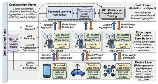
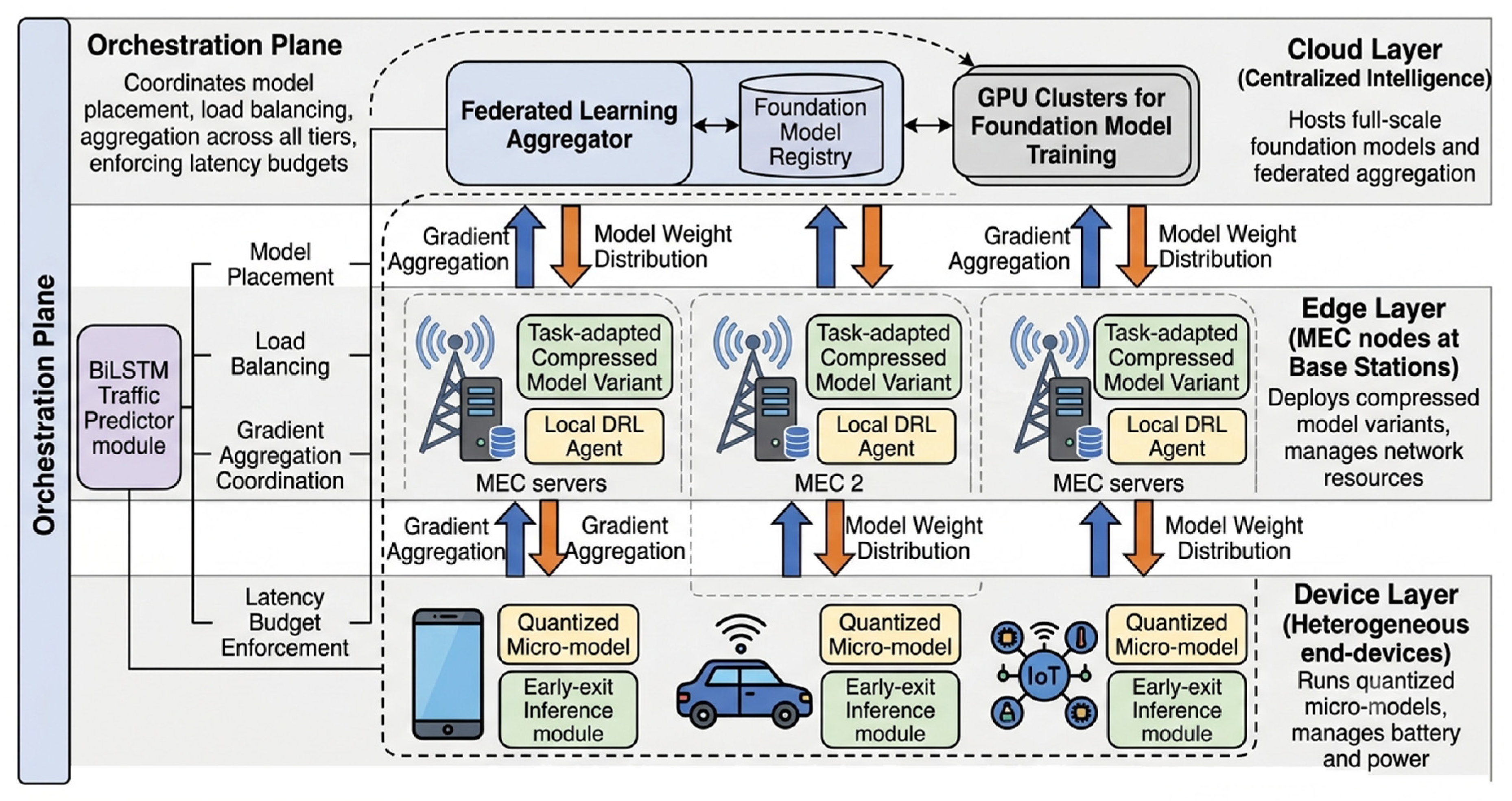
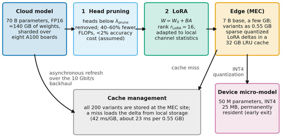
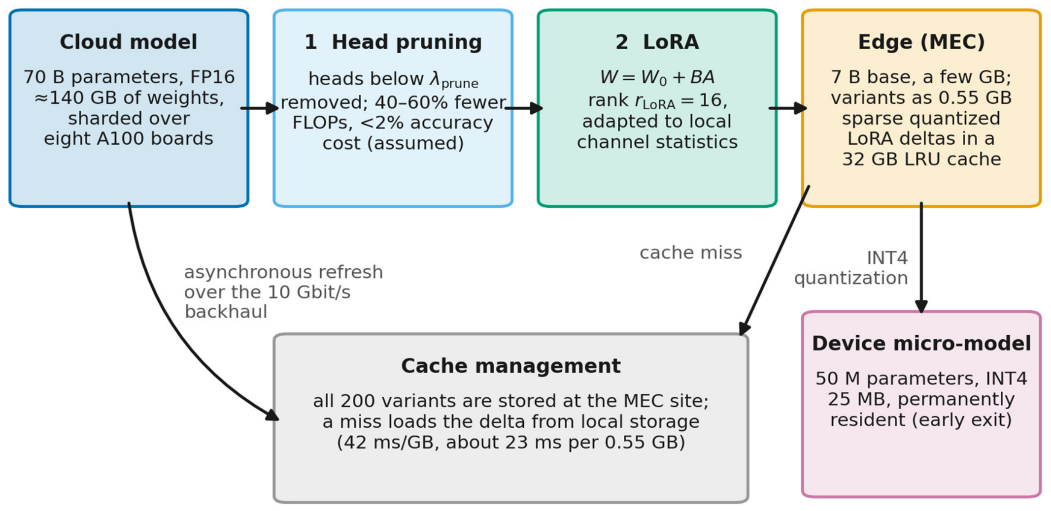
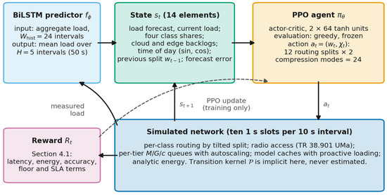
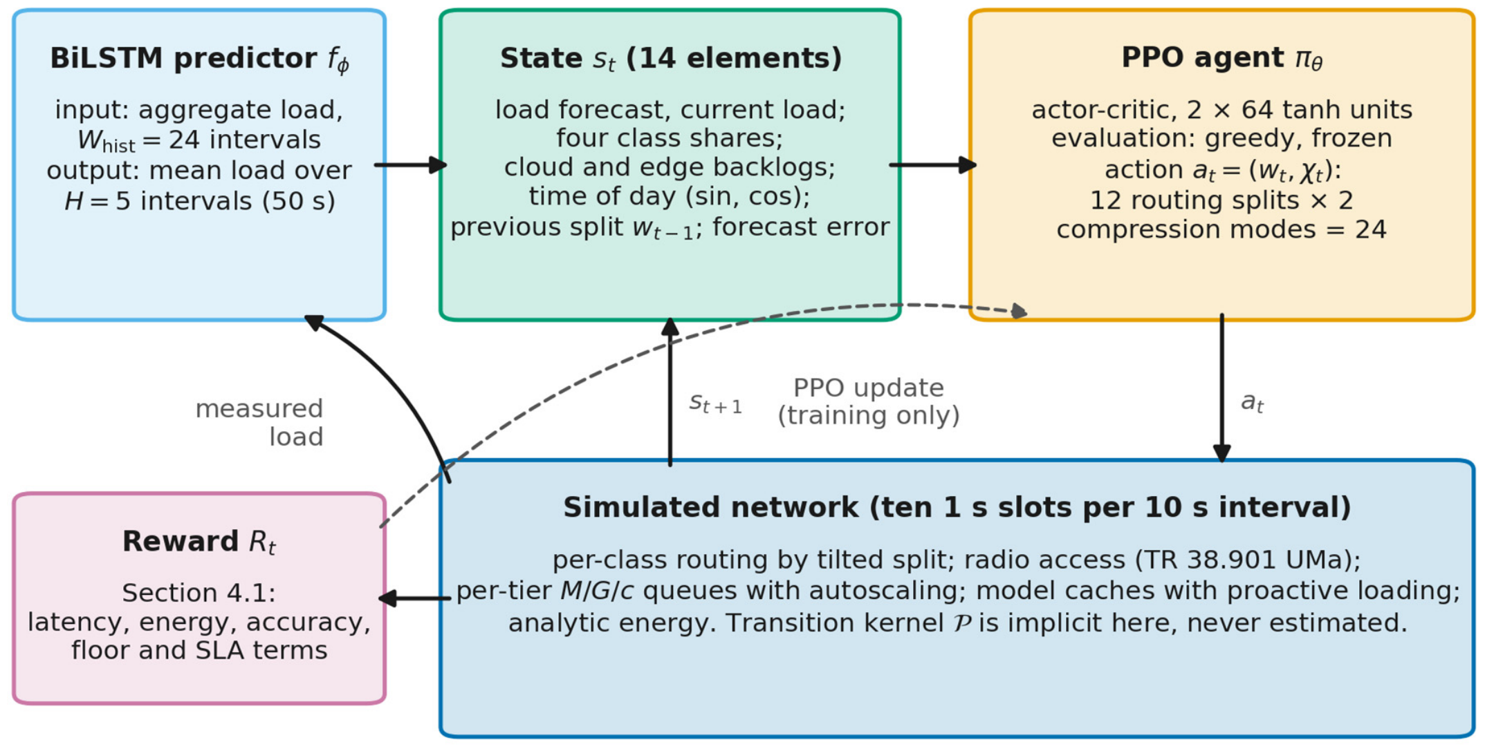
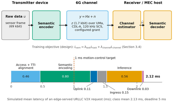
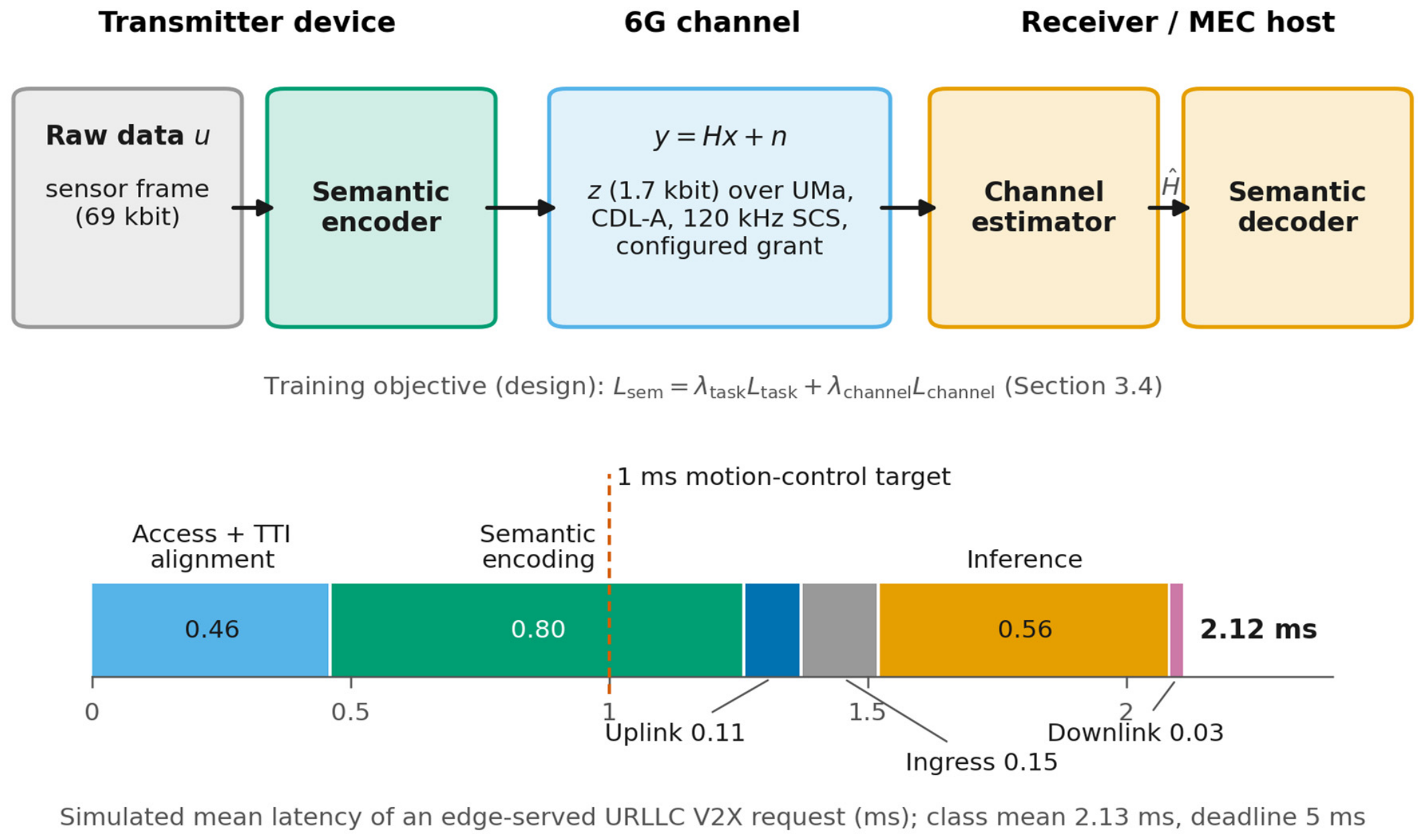
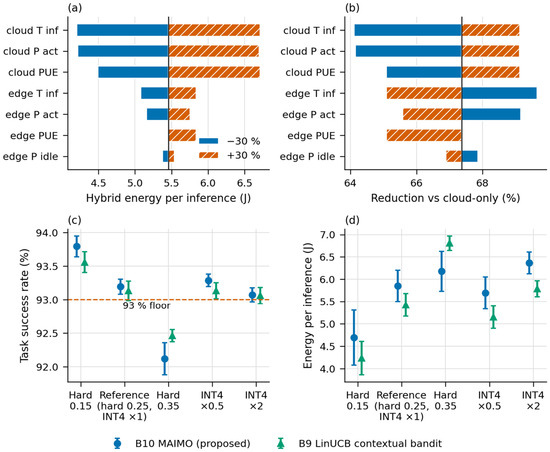
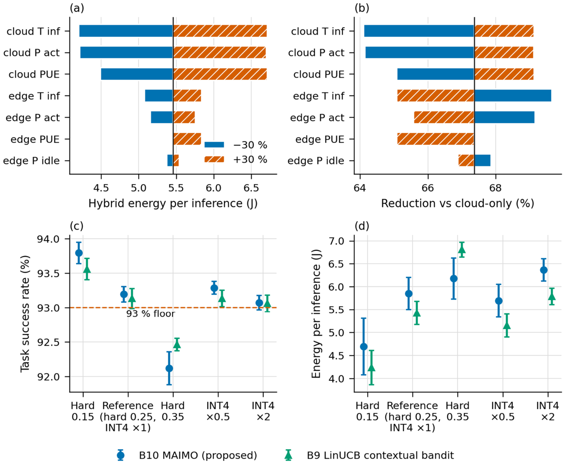
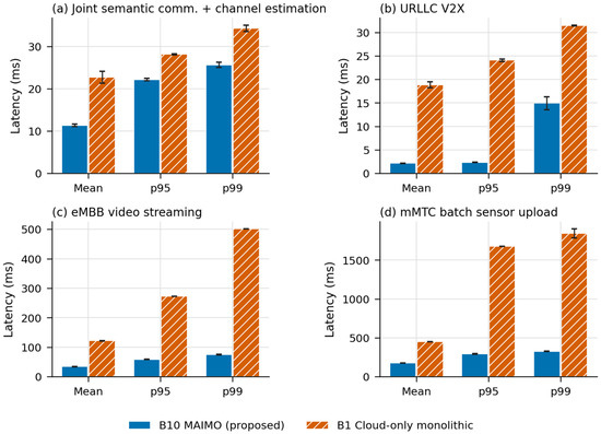
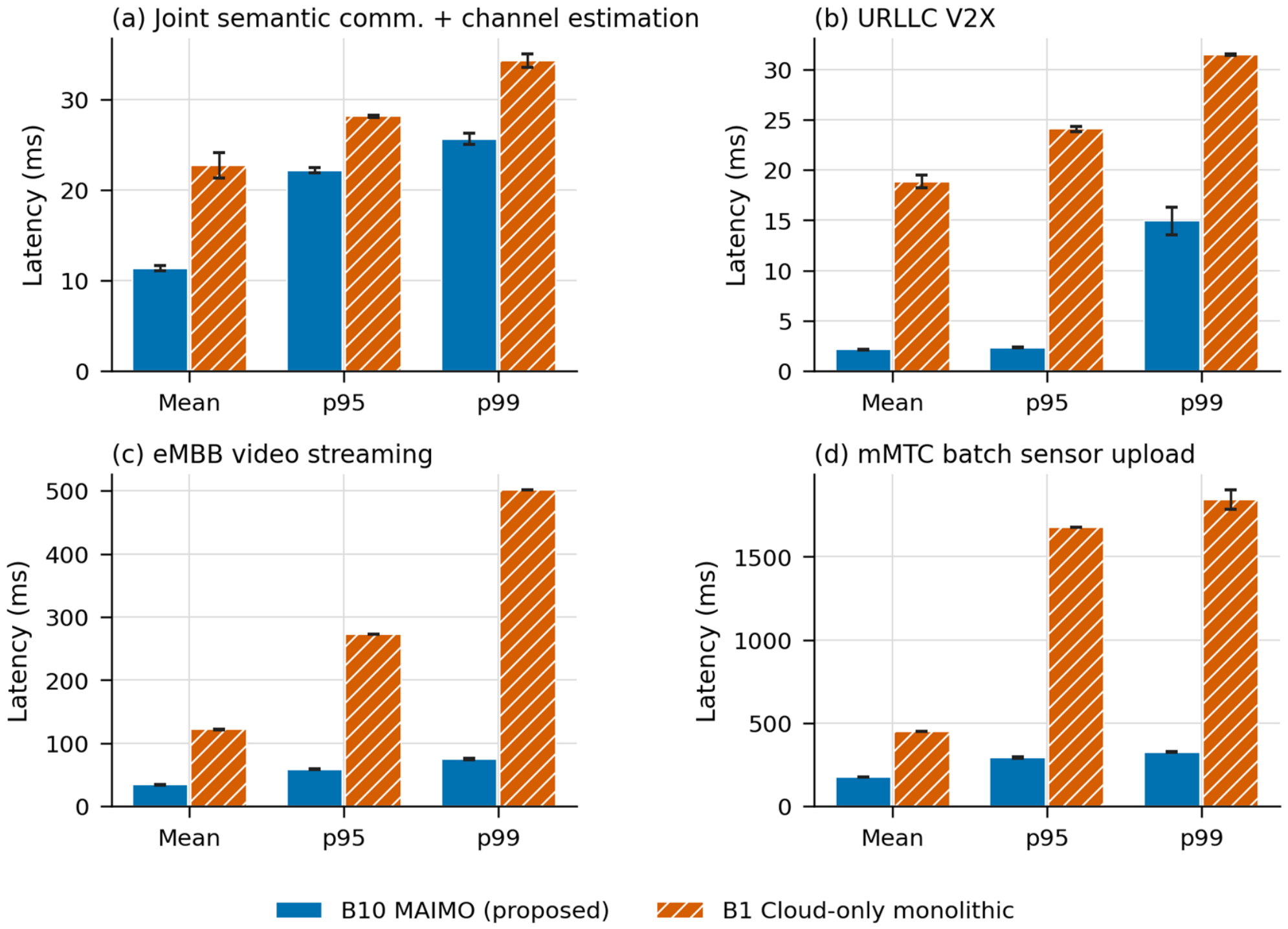
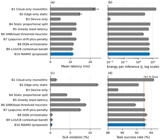
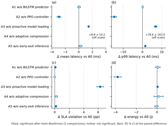
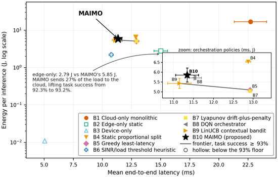
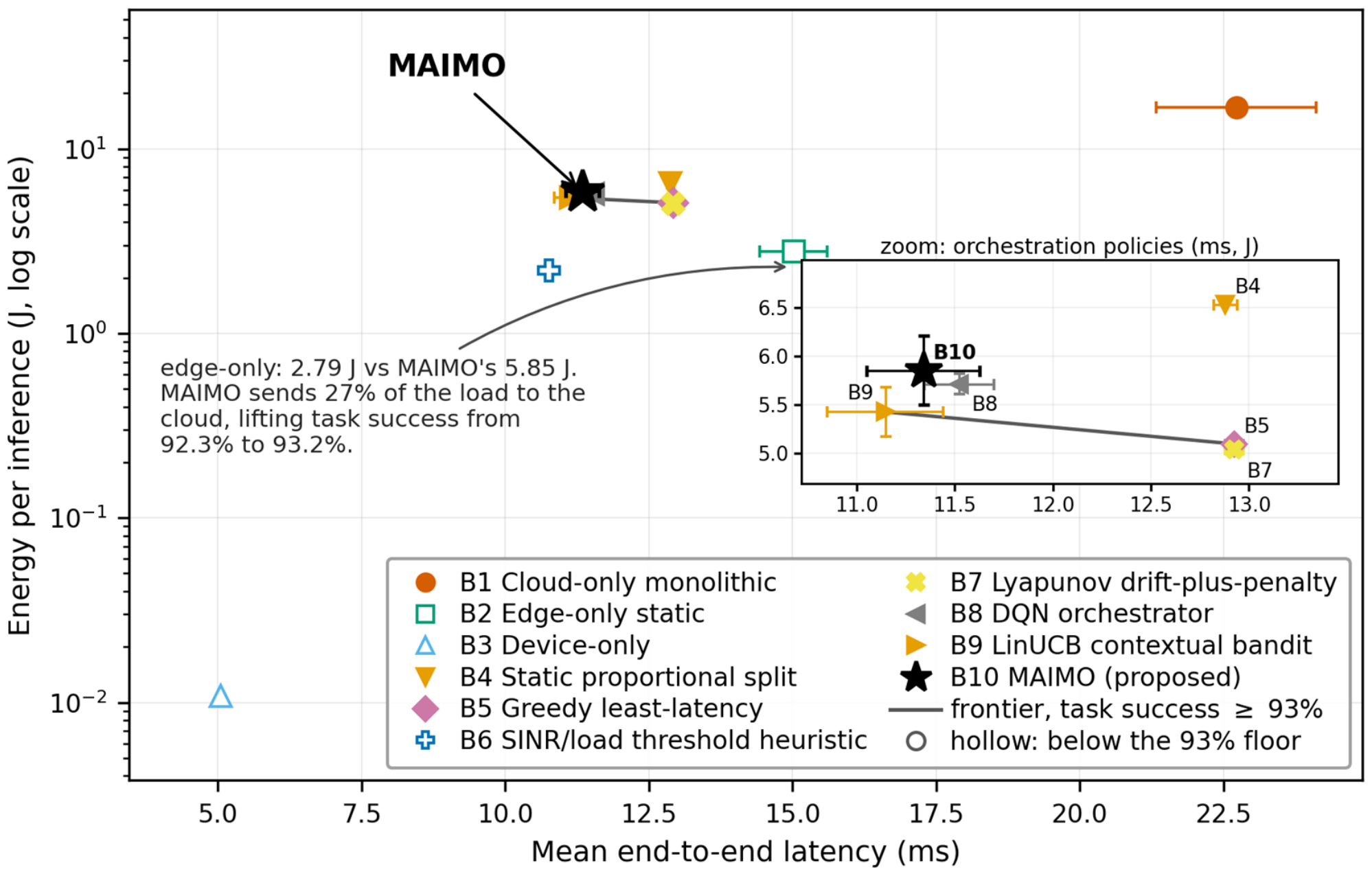
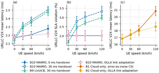
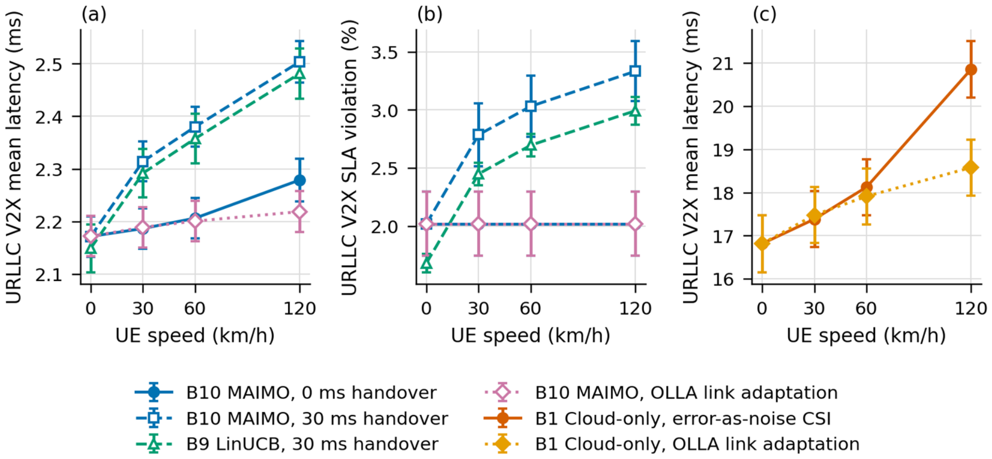
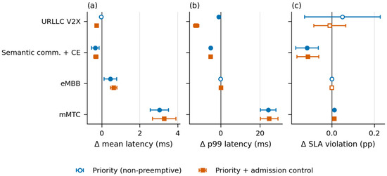
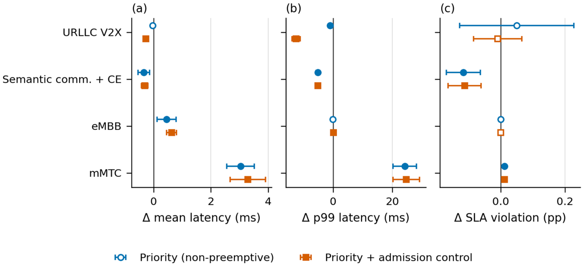
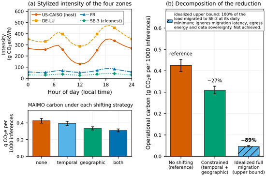
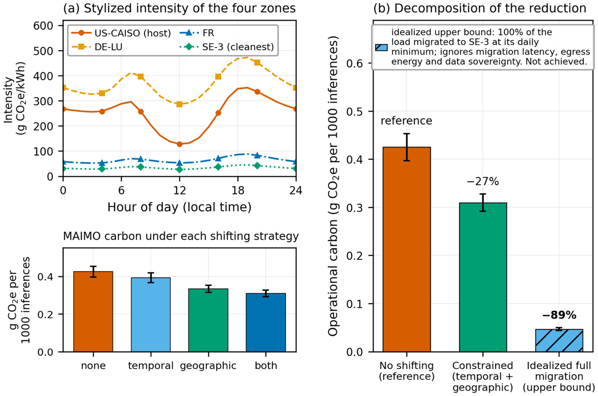

Disclaimer/Publisher’s Note: The statements, opinions and data contained in all publications are solely those of the individual author(s) and contributor(s) and not of MDPI and/or the editor(s). MDPI and/or the editor(s) disclaim responsibility for any injury to people or property resulting from any ideas, methods, instructions or products referred to in the content. |
© 2026 by the authors. Licensee MDPI, Basel, Switzerland. This article is an open access article distributed under the terms and conditions of the Creative Commons Attribution (CC BY) license.