


Abstract
Vessels disabling their Automatic Identification System (AIS) transponder evade AIS-based analytics. We present a framework for maritime dark-vessel screening—auditable candidate attributions for analyst review—coupling synthetic aperture radar (SAR) detection, AIS–SAR association, open-source intelligence (OSINT), and social network analysis (SNA). A Dynamic Kinematic Gate (DKG) grows its radius with speed and AIS staleness, up to 50 km, and demotes stale unmatched AIS to a low-confidence class. On 200 synthetic scenes, it raises true-match recall from 0.65 (capped static gate) to 0.88 and cuts spoofing alerts 4.1-fold via demotion; a fixed 10 km gate reaches 0.91 with fewer false confirmations, so the ceiling needs re-tuning. Re-benchmarked on five seeded SSDD folds with one evaluation code, YOLOv8s, YOLOv10s, and YOLOv11n reach a ship-class average precision (AP@0.50) of 0.940–0.955, on par with the deployed detector SLA-Net (Faster R-CNN with mask-attention and transformer modules; 0.938–0.941), whose two modules bring no significant gain. Without retraining, SLA-Net fails on inshore scenes of two other datasets (AP@0.50 ). On a 12-day operational corpus the static-gate pipeline logs 3190 confirmed matches and 1606 dark detections; OSINT registry documents agree with the AIS-declared name for 90.1% and the flag for 71.8% of 2000 sampled vessels (consistency, not accuracy); a real one-month SNA graph shows no distinct bridge vessel. Attribution remains an analyst-adjudicated judgment.
1. Introduction
International regulations oblige vessels over 300 gross tons on international voyages to operate an Automatic Identification System (AIS) transponder that broadcasts identity and position without interruption [1]. Virtually every maritime domain awareness (MDA) analytic—from trajectory forecasting to behavioral anomaly detection—is built on the assumption that these cooperative broadcasts are present. Such methods, however, share a structural blind spot: they can only reason about vessels that are broadcasting. A vessel that switches its transponder off—whether through equipment failure or deliberate suppression to conceal position, cargo, or destination—disappears from every AIS-only analytic.
Non-cooperative sensing is therefore essential. Space-borne synthetic aperture radar (SAR) images vessels day or night and through cloud, independent of any transmission from the target. In a 12-day operational window over key Indo-Pacific and Middle Eastern corridors, the bidirectional fusion stage logged 3217 confirmed SAR–AIS matches and 1720 dark contacts, radar detections that had no AIS partner within the legacy static gate of that run (Section 4.2). These dark contacts, roughly one in three of the fusion-entered radar detections, are candidates for analyst review rather than confirmed non-broadcasting vessels, because a static gate can miss true AIS partners (Section Association Baselines and Gate Sensitivity). Detecting such a contact, however, is only the first step. Attribution—resolving who the vessel is, who owns it, and whether it belongs to a wider network of shell companies and shadow-fleet registries—is the harder and operationally decisive problem, and it cannot be solved from a radar echo alone.
Three obstacles stand between a SAR detection and an actionable dark-vessel alert. First, association: a SAR detection must be matched to the correct AIS track (or determined to have none). Prior AIS–SAR fusion relies on static distance gates of 2–5 km [2,3]; such a gate is simultaneously too small for fast vessels whose last AIS report is hours stale and too large in dense port approaches, where it merges unrelated contacts. The Dynamic Kinematic Gate proposed here therefore grows the acceptance radius with AIS staleness, but only up to a fixed ceiling km, which a vessel at the assumed maximum surface speed kn (15.43 m/s) reaches after about 0.9 h of AIS silence (Section 3.3). Longer gaps are not absorbed by enlarging the radius. Instead, an AIS broadcast left unmatched after assignment whose last report is more than 3 h older than the SAR pass is routed to a low-confidence temporal-sparsity class, rather than raised as a spoofing alert, whenever a SAR detection lies within the distance the vessel could have covered at (Section 3.4). Association radius and alert triage are thus separate mechanisms: a vessel that may legitimately have moved several hundred kilometers during a multi-hour gap is neither force-matched within the gate nor reported as a spoof. In the controlled evaluation of Section Association Baselines and Gate Sensitivity, the alert reduction is produced by this triage rule, not by the enlarged radius, and wide gates carry a measurable cost in false confirmations. Second, identity: association to a track yields an MMSI, but AIS identity is self-declared and readily falsified. Third, operator overload: under a static gate, the operational run produced more than 105,000 spoof candidates. We attribute this flood mainly to the time gap between the SAR pass and the last AIS position available to the platform, rather than to spoofing; the attribution is consistent with the controlled evaluation of Section 4.3 but was not verified record by record. Such a flood buries the few genuine threats.
This paper addresses all three obstacles with a single, auditable pipeline (Figure 1) and makes the following contributions.
Figure 1.
End-to-end dark-vessel screening pipeline. Numbered stages: (1) Sentinel-1 SAR acquisition; (2) AIS ingestion and kinematic interpolation; (3) SLA-Net detection; (4) bidirectional Hungarian matching with the Dynamic Kinematic Gate; (5) OSINT enrichment; (6) Social Network Analysis; (7) analyst dashboard with human-in-the-loop review. Stage labels reflect the deployed implementation.
- A deployed Sea–Land-Aware detector design (SLA-Net), evaluated. SLA-Net augments a Faster R-CNN backbone with per-level Hierarchical Mask Attention (HMA) and a Global Transformer Bridge (GTB) for scene context and is deployed in the operational pipeline. A seeded five-fold ablation of the two modules (Faster R-CNN, +HMA, +GTB, and +HMA+GTB), with per-fold results, precision–recall curves, operating points, and latency, finds no significant benefit from either module: the ship-class AP@0.50 lies between 0.938 and 0.941 for all four configurations, and no paired comparison is significant after Holm correction (Section 4.1.1). A unified re-benchmark of YOLOv8s, YOLOv10s, YOLOv11n, and RT-DETR-l on the same folds with the same evaluation code places the backbone on par with the three YOLO models, which reach a ship-class AP@0.50 of 0.940–0.955; Faster R-CNN leads only in the three-class mAP, through the two rare population classes (Section 4.1.2).
- A Dynamic Kinematic Gate (DKG) for bidirectional Hungarian AIS–SAR association whose acceptance radius scales with vessel speed and AIS staleness under a physically defensible ceiling, combined with a temporal-sparsity rule that demotes stale unmatched AIS broadcasts. In a controlled, reproducible evaluation on 200 synthetic scenes, the DKG improves true-match recall by 23 percentage points over the legacy capped static gate () and reduces spurious spoofing alerts -fold (); the alert reduction is produced by the demotion rule, not by the enlarged radius. Against ten further association baselines and a one-at-a-time parameter sweep, a fixed 10 km gate attains higher recall (0.909) with fewer false confirmations (391 versus 893), identifying the 50 km ceiling as the parameter to re-tune (Section Association Baselines and Gate Sensitivity). Hungarian assignment outperforms greedy nearest-neighbor association in dense clustered scenes (0.853 versus 0.793), but not in the mixed synthetic scenes (0.878 versus 0.903).
- An OSINT attribution layer that resolves a flagged vessel through its IMO number to 1,244,050 typed registry documents (628,718 distinct after removing a duplicate ingestion), and a Social Network Analysis (SNA) layer over five edge types with Louvain community detection, both implemented in the deployed service and characterized here on the operational data. On 2000 sampled vessels, the registry documents agree with the AIS-declared name for 90.1% and with the flag for 71.8% of the vessels whose flags can be compared. The deployed service synchronizes the OFAC sanctions list but does not match vessels against it; two offline name-based screeners recover 51.4% and 67.0% of the listed vessels found by IMO number. Rebuilt with the deployed edge rules over one month of Persian Gulf traffic (27,991 nodes), the SNA graph is dominated by port hubs and contains no distinct bridge vessel, a negative finding that leaves the bridge-vessel signal a design hypothesis. These are consistency, screening, and graph-structure measures, not attribution accuracy (Section 4.7 and Section 4.8).
- An engineering analysis with reproducible controlled evaluations—asymptotic and measured complexity, seeded controlled ablations with per-fold results, error analysis, and operational and ethical safeguards—with a transparent separation of the operational results, which are reported as recorded and could not be re-run, from the controlled evaluations, which were run with fixed seeds and whose scripts are supplied as Supplementary Material.
The novelty is not any single component but their integration: the system implements the loop adaptive (non-static) gated fusion → identity resolution → network context → alert prioritization, with human-in-the-loop review and audit trails; the identity and network stages are characterized on the operational data but not validated against adjudicated outcomes. AIS behavioral classification, trajectory forecasting, and Robust-Z anomaly scoring are treated in the companion paper; this paper is confined to non-cooperative detection, fusion, and attribution.
The remainder of this paper is organized as follows. Section 2 (Related Work) reviews SAR ship detection, remote-sensing foundation models, and AIS–SAR fusion and graph analysis, and identifies the gap addressed here. Section 3 (Materials and Methods) describes the data sources, SLA-Net, kinematic interpolation and the Dynamic Kinematic Gate, bidirectional Hungarian assignment, the OSINT and SNA layers, and the complexity model. Section 4 (Results) reports the detector benchmark, an ablation of the SLA-Net modules, a re-benchmark of the compared detectors under one evaluation protocol, detector latency and a latency-weighted score, the operational fusion outcomes, the controlled evaluations of the gate and the matcher, the measured assignment complexity, the OSINT consistency and sanctions-screening measurements, and the SNA graph of real traffic. Section 5 (Discussion) addresses operational implications, error analysis, a cross-dataset robustness test of the detector, limitations, safeguards, and deployment, and Section 6 (Conclusions) summarizes the findings and future work.
2. Related Work
2.1. SAR Ship Detection and Transformer Detectors
Constant false alarm rate (CFAR) detectors were the production standard for decades, but deep learning now dominates the SSDD and HRSID benchmarks. Recent work refines convolutional detectors for the small-object, low-signal regime typical of Sentinel-1: lightweight YOLO variants for small SAR ships [4], precision-oriented redesigns [5], explicit multi-scale fusion [6], texture-aware convolution with balanced sampling for robustness to speckle and clutter [7], and near-real-time detectors validated on Gaofen-3 [8]. A parallel thread imports Vision Transformer inductive biases into SAR: local-perception-enhanced Swin backbones [9], DETR variants hardened with edge enhancement and dilated context [10], feature-enhancement transformers for oriented multi-category ships [11], and nested/flow-aligned transformers for very small ships [12]. SLA-Net contributes two maritime-specific modules absent from these detectors: a sea–land mask that attenuates land clutter inside the feature pyramid, and a transformer bridge that supplies scene-level context to a two-stage detection head, a design motivated by the expectation that precision, not raw recall, governs downstream fusion quality. Section 4.1.1 tests whether these modules improve detection, and Section 4.1.2 compares the two-stage detector with single-stage and transformer detectors under one evaluation, which does not support that expectation.
2.2. Foundation Models for Remote Sensing and SAR
Self-supervised pretraining increasingly supplies the representation backbone for MDA. Scale-aware masked autoencoding for multiscale geospatial imagery [13], spectral/EO foundation models [14], multimodal Earth-observation models [15,16], and SAR-native pretraining—a general SAR target-recognition model [17], radiometric/scale-aware SAR masked autoencoding [18], and an ocean-scene SAR foundation model [19]—all transfer well to SAR recognition with limited labels. These models improve where and what a ship is, but remain recognition- and detection-centric: none fuse SAR with AIS kinematics, reason about identity laundering, or provide the relational context needed for attribution.
2.3. AIS–SAR Fusion, Multimodal Maritime Intelligence, and Graph Analysis
Classical fusion associates AIS positions to SAR contacts with fixed distance thresholds and bipartite (Hungarian) assignment [2,20]. Recent multimodal work reports high cross-modal association accuracy—optical/SAR fusion surveys and systems [21,22], an improved multi-feature association method for dark-ship detection between remote-sensing images and AIS [3], graph-learning-driven multi-vessel association [23], and adaptive multimodal trajectory prediction [24]. Two recent systems target dark vessels directly. FusionDark [25] probabilistically fuses Sentinel-1 IW GRDH detections with AIS tracks over the North-East Atlantic, is evaluated on the MMDEC benchmark (230 scenes, 13,306 detections, 19.0 million AIS messages, and 25,130 vessels), ranks anomalies (dark vessels, AIS ghosts, and suspicious matches) with a FusionDark Score, analyzes them spatially against marine protected areas and cable infrastructure, and is validated against SECMAR operations. DarkVesselNet [26], available only as a preprint that has not been peer reviewed, combines Sentinel-1 SAR and Sentinel-2 optical imagery through geospatial foundation-model backbones with AIS trajectory and gap reasoning and an anomaly head. A distinct stream applies graph neural networks and complex-network analysis to AIS trajectories and shipping structures: hybrid GNNs for behavior recognition [27], temporal graph convolutional networks for congestion and prediction [28], community analysis of shipping networks [29,30], and route/pattern mining from massive AIS [31,32,33,34]. Surveys confirm multimodal fusion and anomaly detection as the field’s frontier [35,36].
Table 1 situates representative recent work along the dimensions that matter for dark-vessel attribution. Two gaps recur. First, image/AIS fusion terminates at detection or association: it answers “is there a vessel and which track is it,” not “who is it and what network does it belong to.” Second, the graph/network stream characterizes aggregate traffic or trade communities rather than resolving the identity of a specific suspicious hull. These two dark-vessel systems are the closest to the present work, yet neither performs identity attribution or network analysis: FusionDark scores SAR–AIS correspondences probabilistically rather than through an explicit gate that adapts to vessel speed and AIS staleness, and DarkVesselNet is detection-centric, with AIS used for trajectory and gap reasoning rather than for identity resolution. No prior system among those reviewed integrates adaptive gated fusion, OSINT-based identity attribution, and SNA network context end to end, through to auditable, alert-suppressed operator decisions. This work implements that integration; its identity and network stages are characterized but not validated against adjudicated outcomes.
Table 1.
Representative recent work versus the capabilities required for end-to-end dark-vessel attribution. A check (✓) denotes explicit support; a dash (—) denotes not addressed. “Adaptive gate” denotes a non-static association gate.
3. Materials and Methods
The end-to-end pipeline is shown in Figure 1 (Section 1). Two acquisition streams (SAR and AIS) feed non-cooperative detection (SLA-Net) and cooperative position estimation (kinematic interpolation); a Dynamic Kinematic Gate and Hungarian assignment fuse them into five outcome classes; flagged contacts pass to OSINT enrichment and Social Network Analysis; and results surface on an analyst dashboard with audit trails. All components run against a single PostgreSQL/PostGIS/TimescaleDB store.
3.1. Data Sources and Infrastructure
SAR. Sentinel-1 Ground Range Detected (GRD) imagery is acquired via EODAG from the Copernicus Data Space Ecosystem [37]. Acquisitions in VV polarization are converted to -pixel tiles with a 100-pixel overlap (stride 412 pixels, that is, an overlap of about 20%). In the API service pipeline, a rasterized land–sea mask (1 = sea, 0 = land) is generated for each tile and passed to SLA-Net’s Hierarchical Mask Attention (Section 3.2), tiles whose land fraction exceeds 80% are skipped, and detections whose centroids fall on land are removed after inference. In the batch processing script and in the standalone inference module, by contrast, an all-ones mask is passed to the attention module, so no land suppression is applied inside the network on those paths; the service also falls back to an all-ones mask when the coastline data are not loaded. SAR detections are stored with geographic coordinates, confidence scores, and bounding-box dimensions; the operational run logged 4937 detections that entered bidirectional fusion (3217 confirmed matches and 1720 dark; Section 4). Which of the two code paths produced these detections was not logged.
AIS. AIS data come from a commercial aggregator in two forms. The operational fusion used the live polling tables collected over 5–17 March 2026, which hold 134,470,859 position snapshots of 1,921,466 MMSIs; a snapshot is the aggregator’s latest known position of a vessel at the time of a request, and a vessel is re-polled a median of every 3.8 h, so the last AIS position available at a SAR pass can be hours old. The SNA analysis of Section 4.8 uses the second form, a history backfill of per-vessel position histories (each record a request covering about one month) with positions from December 2025 to early March 2026 and a median of 30 min between consecutive positions; from it, all positions of February 2026 inside two regional boxes were extracted and de-duplicated (Table 18). A Kinematic Interpolator dead-reckons each vessel to its estimated position at the SAR capture time using speed over ground (SOG) and course over ground (COG); the Circular Error Probable (CEP) of each estimate grows with SOG and elapsed time.
OSINT. A corpus of 1,244,050 typed documents is stored in a PostgreSQL JSONB table, keyed by the IMO number of the vessel (company records by company name or company IMO number); Table 2 lists the inventory by report type. The corpus holds nearly every document twice, from two ingestions on 4 and 17 March 2026 (618,593 and 625,457 rows), so 49.5% of the rows are duplicates and 628,718 payloads are distinct within their report type. The report types correspond to port-state-control, ownership, class, and casualty records of the kind published by registries such as Equasis [38], but the source registry of individual documents was not recorded. The service also downloads the public OFAC Specially Designated Nationals (SDN) list [39]; as Section 3.5 explains, it does not match vessels against it.
Table 2.
OSINT corpus document inventory by report type. “Documents” counts corpus rows; “Distinct” counts distinct payloads within each report type, since nearly every document was ingested twice (4 and 17 March 2026).
3.2. SLA-Net: Sea–Land-Aware SAR Ship Detection
SLA-Net extends Faster R-CNN [40] with a ResNet-50 backbone and a Feature Pyramid Network (FPN) [41] producing maps , augmented by two maritime-specific modules.
Hierarchical Mask Attention (HMA). A binary sea–land raster (1 = sea, 0 = land) accompanies each tile. At FPN level l, with feature map of channels, is resized to the spatial size of by nearest-neighbor interpolation, giving . A per-image scalar gain is predicted from the feature map itself: an adaptive average pool of is flattened and passed through a two-layer MLP, –GELU–, followed by tanh,
and the feature map is modulated element-wise as
so that sea-region activations are scaled by and land-region activations by before the region proposal network. HMA is applied independently at the four FPN levels –, each with its own MLP. With an all-ones mask (), Equation (2) reduces to a uniform gain with no spatial land suppression. The original training script applies HMA only during training, whereas the deployed inference module applies it whenever a mask is supplied. The ablation of Section 4.1.1 applies HMA in both training and inference and, because SSDD provides no land raster, with an all-ones mask for every image.
Global Transformer Bridge (GTB). The coarsest level is flattened into a sequence of spatial tokens and passes through a single Transformer encoder layer [42] (, eight heads, feed-forward dimension 1024, GELU activation, dropout 0.1), whose output is reshaped and added back to as a residual, , injecting scene-level context—open-ocean clutter versus a vessel-dense port approach—into the per-proposal classifier. The detection head follows the standard region proposal network, ROI Align, and box predictor. Figure 2 shows the architecture.
Figure 2.
SLA-Net architecture. At every FPN level (–), Hierarchical Mask Attention computes a scalar gain from the feature map itself (7 × 7 average pooling, a two-layer MLP, and tanh) and modulates the feature map element-wise by the sea–land mask resized to that level (Equations (1) and (2)). The Global Transformer Bridge, a single Transformer encoder layer, is applied to only and added back as a residual, , before the Faster R-CNN detection head.
3.3. Kinematic Interpolation and the Dynamic Kinematic Gate
Given a last reported position , SOG v, and COG , the dead-reckoned position at is and with km. The acceptance gate for AIS vessel j is
where is the AIS staleness of vessel j in seconds. All lengths in Equation (3) are in meters. Speeds are reported in knots (kn, the nautical unit of speed; 1 kn m/s), and enters the staleness term converted to meters per second, kn m/s, so that is a distance in meters: one hour of AIS silence ( s) adds m to the radius before the ceiling applies. Table 3 lists every symbol with its value, unit, and implementing code constant. The reference speed kn makes the argument of the square root dimensionless, so that is a length that absorbs speed-dependent position noise; the term absorbs dead-reckoning uncertainty. The floor m corresponds to about 20 pixels at the 10 m pixel spacing of Sentinel-1 IW GRD products; it is not a resolution limit but a minimum allowance for residual geolocation error, tile-stitching offsets, and short-horizon dead-reckoning error. The term grows the gate as fast as a surface vessel at the assumed maximum speed could travel, so that a genuine but stale track is not spuriously declared a spoof, and the fixed ceiling km keeps the cost matrix sparse and the Hungarian assignment tractable. From the 200 m floor, the ceiling is reached when km, that is, after s (about 0.9 h). Staleness beyond that point is handled by alert triage rather than by the radius: an AIS broadcast left unmatched after assignment whose staleness exceeds the temporal-sparsity threshold of 3 h is demoted to the low-confidence temporal-sparsity class under the rule given in Section 3.4, instead of being raised as a spoof candidate. Equation (3) replaces the static 5 km threshold of prior work [2,3]. In the implementation, the legacy static configuration, used as the baseline in Section 4.3, is invoked when no SAR capture time is supplied; it evaluates , that is, the same floor terms capped at 5 km, with no staleness term and no temporal-sparsity demotion. Its radius therefore equals 5 km only when km and is otherwise the floor term.
Table 3.
Parameters of the Dynamic Kinematic Gate (Equation (3)) and of the temporal-sparsity rule, with units and the constants that implement them in api/services/sar_correlator.py. All lengths are in meters and all times in seconds; speeds are given in knots and are converted to m/s in the staleness term.
3.4. Bidirectional Hungarian Assignment
For a scene with m SAR detections and n AIS interpolations, the cost matrix is if and ∞ otherwise, where is the great-circle distance. The matrix is square-padded to and solved with the Jonker–Volgenant algorithm (scipy.optimize.linear_sum_assignment); pairs with after assignment are confirmed. In the implementation, out-of-gate and padding cells carry the large finite cost rather than ∞; the solver therefore first maximizes the number of in-gate pairs and only then minimizes the summed normalized distance, which matters when gates are wide (Section Association Baselines and Gate Sensitivity). Every SAR detection and every unmatched AIS broadcast receives exactly one of five outcome labels (Figure 3):
Figure 3.
(a) Illustrative cost matrix for a scene; cells outside the Dynamic Kinematic Gate are left blank, and the green outline marks the optimal assignment returned by scipy.optimize.linear_sum_assignment. (b) Gate radius versus AIS staleness for a vessel at SOG kn with , computed with the production gate function (_gate_for in sar_correlator.py); the radius reaches the 50 km ceiling after about 54 min. The dashed red line is the 5 km cap of the legacy capped static gate, and the dashed vertical line marks the 3 h temporal-sparsity threshold beyond which unmatched AIS are demoted rather than alerted.
- Confirmed: SAR↔AIS matched within the gate.
- Dark: SAR detection with no AIS within the gate.
- Spoof candidate: AIS broadcast with no SAR echo that is not demoted under item 5 (in particular, every unmatched broadcast with h).
- Identity laundering: matched AIS declaring Pleasure/Fishing/Class-B while the SAR bounding box exceeds 50 m—a physical-truth override, since a declared small craft cannot be 180 m long.
- Low-confidence temporal sparsity: unmatched AIS with h for which at least one SAR detection in the scene lies within the uncapped reachable radius (or the scene contains no SAR detection)—demoted from the operator view as a satellite-cadence artifact rather than a threat.
3.5. OSINT Attribution and Social Network Analysis
Once flagged, a vessel is resolved in five steps, as implemented in the deployed service: (i) the IMO number is read from the vessel-static record of its MMSI; (ii) all corpus documents keyed on that IMO number are retrieved and grouped by report type; (iii) the OFAC SDN list [39] is downloaded and kept synchronized, but no step compares vessels with it, so sanctions status is not part of the dossier; (iv) maritime news is collected from RSS feeds for the analyst, without automatic linkage to the vessel; and (v) the documents, the vessel’s behavioral anomalies, its SAR correlations, and its watch-list status are aggregated into a dossier. The dossier returns the report type and payload of each document, but not its source registry or URL, which were not recorded, nor its ingestion time, which is stored but not returned; the evidence trail therefore reaches the report type, not the individual source.
The SNA graph is built over five edge types, whose deployed rules are as follows. Ship-to-ship (STS) transfer: two vessels with SOG kn (a missing SOG counts as 0) whose latest positions in the same 5 min time bucket lie within 1 km, with at least 0.5 h between the first and the last shared bucket, which need not be consecutive; pairs whose mean position lies within 2 nautical miles of a port are excluded, and at least one vessel must have a cargo or tanker type, or the types of both must be unknown. Port call: a vessel–port edge when at least three positions of the vessel with SOG kn lie within 3704 m (2 nautical miles) of a port with a UN/LOCODE; these are vessel–port edges, not vessel–vessel co-visits, and three such ports lack coordinates and cannot receive edges. Ownership: vessel–company and company–company edges extracted from the ownership and company documents after company names are canonicalized and merged by fuzzy string matching (token-sort ratio ), which can join distinct companies with similar names. Flag: vessel–flag edges seeded from a country_iso field of the vessel-static record, which no exported record carries, so the deployed code creates no flag edges on these data. Dark proximity: pairs of vessels with SAR correlations of confidence whose last AIS positions lie within about 50 nautical miles and 24 h of each other, which requires the SAR correlation tables. Ego-networks expand breadth-first from a seed MMSI over a default look-back window of 720 h (30 days); the default depth is two hops and the service accepts at most three. Graphs larger than the node cap (default 3000 nodes) are truncated to the highest-degree nodes, always retaining the seed. The HTTP endpoint omits flag edges unless they are requested. Louvain modularity optimization [43] (fixed random state 42, with connected components as a fallback partition) partitions the graph, and two centralities are computed with NetworkX [44]: degree centrality and betweenness centrality estimated from sampled source nodes with a fixed seed (42). Closeness and PageRank centralities are not computed by the deployed service. A bridge vessel—high betweenness linking otherwise disconnected communities—is the signal the layer was designed to surface; Section 4.8 tests whether such a vessel appears in real data.
3.6. Complexity and Cost Model
Table 4 gives the asymptotic cost of each stage. Detection scales linearly in the number of tiles; gating is quadratic in per-scene cardinality; Hungarian assignment is in the worst case (empirically sub-cubic here, Section 4.5); OSINT is linear in the number of flagged contacts under indexed lookup; and SNA is dominated by sampled betweenness. Because scenes are small (N of order tens) and the ego-network is capped, the pipeline is dominated in practice by SAR inference, not by fusion or graph analysis.
Table 4.
Per-stage computational cost. T = SAR tiles; = SAR detections and AIS interpolations per scene, ; F = flagged contacts; = SNA graph nodes and edges; k = betweenness sample size.
3.7. Reproducibility
The controlled experiments of Section 4 (complexity timing and the DKG and matcher ablations) were run with fixed random seed 42 using the deployed matching code (scripts/fusion_experiments.py), and their outputs are recorded as machine-readable tables. The analysis scripts, machine-readable tables, and per-fold results of all experiments run for this study are supplied as Supplementary Material with this submission, and the per-fold results of the detector experiments are also listed in Appendix A. The detector benchmark of Table 5 and the operational 12-day corpus results are reported from the project record, that is, from the original benchmark and operational runs, whose logs and checkpoints were not retained; their values are reported as recorded and are not re-measured here. The SLA-Net ablation, the detector latency measurements, and the detector failure analysis (Section 4.1.1, Section 4.1.3 and Section 5.2) were run for this revision with seed for fold f (scripts/slanet_ablation.py and scripts/slanet_failure_cases.py), and their per-fold results are kept as machine-readable tables. The re-benchmark of YOLOv8s, YOLOv10s, YOLOv11n, and RT-DETR-l (Section 4.1.2) was run on the same folds with the same seeds (scripts/detectors_kfold.py), and its per-fold results, precision–recall curves, and training settings are kept in the same way. The cross-dataset test of Section 5.3 applies the 20 checkpoints of that ablation in inference only (scripts/crossdataset_eval.py), and its per-fold results are kept in the same way. The OSINT and SNA analyses of Section 4.7 and Section 4.8 were run on a CPU over the exported operational data with the deployed graph-construction code imported unmodified, with fixed seeds for vessel sampling, Louvain partitioning, and betweenness sampling (all 42).
Table 5.
SSDD five-fold SAR ship-detection benchmark (mean ± SD across folds). Best per column in bold. Values are from the project record and were not re-measured. Recall is the Ultralytics recall at IoU 0.50 for the YOLO and RT-DETR models but mAR@100, averaged over IoU 0.50–0.95, for Faster R-CNN and RetinaNet, so the column is not comparable across these groups (Section 4.1.2). YOLOv8s, YOLOv10s, YOLOv11n, and RT-DETR were re-trained and re-scored under the unified protocol of Section 4.1.2; RetinaNet was not re-run.
4. Results
4.1. SLA-Net Detector
In the five-fold benchmark on SSDD [45] of the project record (Section 3.7), which was not re-run, a Faster R-CNN detector attains the highest mAP@0.50 () and the highest strict-IoU score, mAP@[0.50:0.95] (), in the benchmark (Table 5), leading YOLOv8s by 10.4 and YOLOv11n by 12.1 percentage points on the strict multi-IoU metric. This Faster R-CNN detector is the backbone of the deployed SLA-Net (Section 3); its HMA and GTB modules are used operationally but are not isolated in this benchmark, so the reported figures reflect the backbone rather than the augmented model; the modules are ablated in Section 4.1.1. The Faster R-CNN choice was motivated by the expectation that the YOLO variants trade precision for recall and that precision governs downstream fusion quality, because a false SAR detection entered into the Hungarian matrix creates a spurious dark or spoof outcome. This expectation is not supported by the re-benchmark of Section 4.1.2: the recall column of Table 5 mixes two definitions, the benchmark recorded no precision for Faster R-CNN, and on the folds and with the evaluation code of this study the YOLO models are more precise than Faster R-CNN at a score threshold of 0.5 and within 0.028 of it in maximum F1. The values of Table 5 are kept as the project record. Reporting variance across folds is deliberate: RetinaNet’s collapse () is invisible under the single-split reporting common in prior work.
4.1.1. Ablation of the HMA and GTB Modules
To isolate the contribution of the two SLA-Net modules, four configurations were trained and evaluated under one protocol: (A) Faster R-CNN with a ResNet-50 FPN backbone, (B) A with HMA, (C) A with GTB, and (D) A with both modules, which is the deployed SLA-Net architecture. The HMA and GTB classes were imported unmodified from the original SLA-Net training code. The 1160 SSDD images were pooled, sorted by file name, and split into five folds (shuffled with seed 42; 928 training and 232 validation images per fold), with the three classes of the benchmark (ship, small population, and large population; 2587, 136, and 21 boxes in total). Every run started from an ImageNet-initialized backbone and used the seed for fold f in all random-number generators, so that the four configurations saw the same data order within a fold. Training used stochastic gradient descent (learning rate 0.005, momentum 0.9, weight decay , no learning-rate schedule, and no data augmentation), mixed precision (fp16), and batches of four images with two-step gradient accumulation, for at most 25 epochs. After each epoch the model was evaluated in inference mode, and the checkpoint with the highest validation mAP@0.50 was kept, with early stopping after six epochs without improvement.
The protocol deviates from that of the benchmark in Table 5 in ways that apply identically to all four configurations but make the absolute values incomparable with that table. Images were resized to pixels instead of the default resize. Training was capped at 25 epochs instead of 150, and 11 of the 15 runs of configurations A–C reached the cap, with best epochs between 16 and 25, so these models were probably still improving. The fold membership differs from that of the benchmark, whose file order cannot be recovered. Unlike the original training script, the ablation applies HMA in inference as well as in training, as the deployed inference module does. The checkpoint was selected by validation mAP@0.50 on the same fold on which it is reported, instead of by the lowest training loss, so the values in Table 6 are optimistically biased; the last epoch, which had the lowest training loss in every run, gives lower mAP@0.50 values (A 0.703, B 0.731, C 0.741, and D 0.676). Finally, SSDD provides no land raster. An Otsu-threshold proxy mask was tested and rejected, because it labeled 518 of the 2587 ground-truth ship centers (20.0%) as land and marked open-sea scenes with a brightness gradient as land. An all-ones mask was therefore used for every configuration, under which Equation (2) reduces to a learned per-level gain : configurations B and D test that gain, not spatial land suppression.
Table 6.
Five-fold ablation of the SLA-Net modules on SSDD (mean ± SD over five folds; seed for fold f; input; best-validation checkpoints; all-ones sea–land mask). mAP and mAR are averaged over the three classes; the ship columns refer to the ship class only; F1 is for the ship class at IoU 0.50 and a score threshold of 0.5. Configuration D is the deployed SLA-Net architecture. Because checkpoints were selected on the reporting fold and the protocol differs from that of Table 5, the values are not comparable with that table. No difference from A is significant after Holm correction.
Table 6 and Figure 4 report the results, and Table A1 in Appendix A lists them per fold. On the ship class, which holds 2587 of the 2744 boxes, the four configurations are practically indistinguishable: AP@0.50 ranges from 0.938 (A) to 0.941 (B), and AP@[0.50:0.95] from 0.595 (D) to 0.619 (B). Paired with A over the five folds, the ship-class AP@0.50 changes by with HMA (, paired t-test), by with GTB (), and by with both modules (). The three-class mAP@0.50 shows a larger difference for HMA (, 95% CI , Cohen’s ; paired t-test , exact Wilcoxon signed-rank test ), but is the smallest p-value that the Wilcoxon test can attain with five pairs, and after Holm correction over the three comparisons with A the two p-values become 0.22 and 0.19. GTB (, ) and the combination of both modules (, ) differ less. No comparison with A is significant after correction for any of the four metrics tested (three-class mAP@0.50 and mAP@[0.50:0.95], and ship-class AP@0.50 and AP@[0.50:0.95]). The Wilcoxon test is reported alongside the t-test because the normality of the paired differences cannot be checked reliably with five pairs (Shapiro–Wilk for the D–A differences in mAP@0.50).
Figure 4.
Five-fold ablation of the SLA-Net modules on SSDD (mean ± 1 SD over folds; seed for fold f; input; best-validation checkpoints; all-ones sea–land mask). Faster R-CNN is configuration A, and +HMA+GTB is the deployed SLA-Net architecture. The three-class differences are driven by the two population classes, with 1–8 large-population boxes per validation fold; the ship-class AP@0.50 differs by at most 0.004 between configurations. Values are those of Table 6.
The three-class gain of HMA is concentrated in the two rare population classes. Relative to A, the AP@0.50 of configuration B rises by 0.206 for large population and by 0.081 for small population, against 0.004 for ship, so the large-population class accounts for about 70% of the . That class has only 21 boxes, with 1, 4, 2, 8, and 6 in the five validation folds, so a single box can move its AP substantially: in fold 1, whose validation set holds one large-population box, the AP@0.50 of that class is 0.333 for A and 1.000 for B, C, and D. The three-class differences therefore rest on a handful of boxes rather than on a systematic effect of the modules.
The ship-class precision–recall curves of the four configurations at IoU 0.50, averaged over the folds, overlap almost completely (dashed curves in Figure 5). At a score threshold of 0.5, the F1 score is for A (precision 0.868, recall 0.936) and for B (precision 0.906, recall 0.931), with C at 0.905 (0.874 and 0.941) and D at 0.901 (0.868 and 0.938); the maximum F1 over all thresholds is 0.925, 0.932, 0.929, and 0.925 for A to D. The slightly higher F1 of B at the default threshold comes from precision rather than recall, and its maximum F1 lies within the fold-to-fold spread of the others. Under this protocol, neither module is shown to improve detection; the deployed SLA-Net rests on its Faster R-CNN backbone (Table 5) rather than on its added modules, and that backbone is on par with, not ahead of, the YOLO models on the ship class (Section 4.1.2).
Figure 5.
Ship-class precision–recall curves at IoU 0.50 of eight detectors: the four re-benchmarked Ultralytics detectors (solid) and the four Faster R-CNN ablation configurations (dashed) on the held-out SSDD folds. For each detector, the interpolated precision of each fold is evaluated on a common recall grid and averaged over the five folds; shaded bands ( SD) are drawn for the Ultralytics detectors only. Dots mark the mean operating point at a score threshold of 0.5. (a) Full range; (b) recall 0.80–1.00. Detections are limited to scores of at least 0.05 for Faster R-CNN and 0.001 for the Ultralytics detectors.
4.1.2. Re-Benchmark of the Compared Detectors Under One Protocol
The single-stage and transformer detectors of Table 5 were trained without seeds, on folds that cannot be recovered, scored with each framework’s own metric code, and their per-fold scores were not retained. For this revision, YOLOv8s, YOLOv11n, and RT-DETR-l, and subsequently YOLOv10s, were retrained on the five folds of the ablation (Section 4.1.1) with the seed for fold f and deterministic training, and their best checkpoints were scored with the evaluation code of the ablation, imported unmodified (torchmetrics, COCO 101-point interpolation, at most 100 detections per image, and ship-class operating points from the same greedy matching at IoU 0.50). RetinaNet was not re-run. Training followed the original benchmark script with four deviations: an epoch limit of 60 in fold 1 and 40 in folds 2–5, reduced after the fold-1 run of RT-DETR-l took 76 min (40 in all five folds for YOLOv10s, trained after this change), against 150 epochs, with a patience of 12 instead of 20 epochs; batches of 16 (YOLO) and eight (RT-DETR-l) images instead of 32 and 16, with gradient accumulation to the same nominal batch of 64; selection of the checkpoint with the highest validation mAP@[0.50:0.95] on the reporting fold, the fitness criterion of this Ultralytics version, instead of the training-log row with the highest mAP@0.50; and evaluation of the checkpoints, stored in fp16, in fp32. In the original runs as in these, the automatic optimizer selection of Ultralytics trained the YOLO models with AdamW at a learning rate of 0.001429 instead of the requested 0.01. Predictions used a score threshold of 0.001, non-maximum suppression at IoU 0.7, and a 640-pixel input, letterboxed for the YOLO models and stretched to by the RT-DETR predictor. YOLOv10s was run with its NMS-free one-to-one head, which keeps at most 300 top-scoring boxes without non-maximum suppression, so the IoU 0.7 setting does not apply to it. The Faster R-CNN configurations share the folds, the seeds, the checkpoint selection on the reporting fold, and the evaluation code, but not the recipe (SGD, pixels, at most 25 epochs, no augmentation, selection on mAP@0.50, and torchvision post-processing with a score threshold of 0.05 and non-maximum suppression at IoU 0.5), so the comparison is between the standard recipes of the two frameworks, scored identically. The lower score threshold of the Ultralytics models only appends lower-scored detections and cannot reduce their average precision, and all values share the optimistic bias of selection on the reporting fold.
Table 7 and Figure 5 report the results (per fold in Table A2). On the ship class, which holds 2587 of the 2744 boxes, the three YOLO models and the four Faster R-CNN configurations lie within 0.02 of each other in AP@0.50 ( for YOLOv8s, for YOLOv10s, for YOLOv11n, and 0.938–0.941 for A–D), so that YOLOv10s is on par with the Faster R-CNN configurations; in ship-class AP@[0.50:0.95], YOLOv11n (0.617) is level with B and C and above A (0.600), and YOLOv8s (0.568) and YOLOv10s (0.563) are lowest. RT-DETR-l is lower and unstable across folds: its ship-class AP@0.50 of is 0.904–0.944 in folds 1–3 but 0.716 and 0.294 in folds 4 and 5, whose runs stopped early after 32 and 30 epochs. The three-class metrics favor Faster R-CNN (mAP@0.50 0.723–0.820 against 0.669, 0.660, 0.611, and 0.299 for YOLOv8s, YOLOv10s, YOLOv11n, and RT-DETR-l; mAP@[0.50:0.95] 0.415–0.444 against 0.369, 0.370, 0.365, and 0.152), but, as in the ablation, the mAP@0.50 ordering is set by the population classes (157 boxes): their AP@0.50 is 0.509 (small) and 0.550 (large) for YOLOv8s, 0.486 and 0.553 for YOLOv10s, and 0.556 and 0.322 for YOLOv11n, against 0.708 and 0.522 for A.
At a score threshold of 0.5, the ship-class precision, recall, and F1 are 0.953, 0.840, and 0.891 for YOLOv8s; 0.950, 0.852, and 0.898 for YOLOv10s; 0.961, 0.860, and 0.907 for YOLOv11n; 0.726, 0.702, and 0.658 for RT-DETR-l; and 0.868–0.906, 0.931–0.941, and 0.901–0.919 for A–D. At 0.25 they are 0.836, 0.928, and 0.879; 0.821, 0.923, and 0.869; 0.846, 0.934, and 0.887; 0.383, 0.914, and 0.527; and 0.800–0.875, 0.944–0.949, and 0.867–0.908. The maximum F1 is 0.909, 0.904, and 0.920 for YOLOv8s, YOLOv10s, and YOLOv11n (at mean thresholds of 0.42, 0.44, and 0.44), 0.750 for RT-DETR-l, and 0.925–0.932 for A–D (at 0.82–0.92). At a common threshold of 0.5, the YOLO models are thus the more precise and the Faster R-CNN configurations the more complete detectors, a difference in score calibration rather than in ranking quality.
Table 8 shows why the absolute values differ from those of Table 5. On the same checkpoints, the three-class mAP@0.50 of the unified evaluation agrees with that of the Ultralytics validator within 0.001 (0.003 for YOLOv10s), and the rule of the original benchmark, applied to this run’s training logs, gives values higher by less than 0.01 (0.021 for YOLOv10s, about half of its gap of 0.041 to the published value). The evaluation code therefore does not explain the gap to the published values (0.752, 0.701, 0.762, and 0.642), which lies mainly in the training runs (Table 9): 150 epochs instead of 40–60, and unseeded training on a different fold partition. The precision and recall columns are not comparable across protocols, because their definitions differ (caption of Table 8). Table 5 mixed these definitions: its recall column holds the Ultralytics recall for the YOLO and RT-DETR models but mAR@100, a stricter quantity averaged over IoU 0.50–0.95, for Faster R-CNN (0.631) and RetinaNet, and the benchmark recorded no precision for either of them. Under a common definition, the mAR@100 of YOLOv8s, YOLOv10s, and YOLOv11n is 0.622, 0.661, and 0.624 (Table 7).
Table 7.
Re-benchmark of the compared detectors on the five SSDD folds of the ablation, scored with one evaluation code (mean ± SD over folds; seed for fold f; checkpoints selected on the reporting fold). mAP and mAR are three-class averages; ship F1 is at IoU 0.50, at a score threshold of 0.5 and at its maximum. Training settings are in Table 9; the Faster R-CNN rows repeat Table 6. YOLOv10s, re-run last, uses its NMS-free head and was trained for at most 40 epochs in every fold.
Table 8.
The Ultralytics detectors under three protocols on the re-benchmark runs, and as published (mean ± SD over five folds). (i) Unified code of Table 7: P is the ship-class precision at score 0.5 and IoU 0.50; R is the three-class mAR@100 (IoU 0.50–0.95). (ii) Ultralytics validator on the same checkpoints: P and R are three-class means at IoU 0.50 at the confidence of maximum mean F1. (iii) Original rule on this run: the training-log row (fp16, moving-average weights) with the highest mAP@0.50; P and R as in (ii). (iv) Rule (iii) on the original runs (150 epochs, unseeded, other folds; population SD). For Faster R-CNN and RetinaNet, the recall of Table 5 is mAR@100 as in (i).
Table 9.
Training details of the detectors of Table 7; f is the fold index. The original benchmark of Table 5 trained the Ultralytics models for up to 150 epochs (patience 20) with batches of 32 (YOLO) and 16 (RT-DETR) images and no seed. YOLOv10s was re-run after the epoch limit had been reduced and was trained for at most 40 epochs in every fold.
The argument of Section 4.1 for choosing Faster R-CNN, that the YOLO models trade precision for recall and that precision governs fusion quality, is therefore not supported. At a score threshold of 0.5 the YOLO models are the more precise (0.953, 0.950, and 0.961 for YOLOv8s, YOLOv10s, and YOLOv11n against 0.868–0.906); at maximum F1, which removes the calibration difference, the Faster R-CNN configurations exceed YOLOv11n by 0.005–0.012, YOLOv8s by 0.016–0.023, and YOLOv10s by 0.021–0.028, of the order of the fold-to-fold SD (0.014–0.025); and in ship-class AP@0.50, YOLOv8s and YOLOv11n are 0.008–0.018 higher, while YOLOv10s is level (0.940 against 0.938–0.941). No significance test was computed, because the recipes differ. The re-benchmark supports that the Faster R-CNN backbone is on par with the three YOLO models on SSDD ships, not that it is more accurate, and that RT-DETR-l is less accurate and less stable under this schedule.
With the trained fold-1 checkpoints, measured as in Section 4.1.3 with no other compute process on the GPU, the end-to-end latency at batch size 1 is ms in fp32 and ms in fp16 for YOLOv8s, and ms for YOLOv11n, and ms for RT-DETR-l, and and ms for YOLOv10s, all within 1.0 ms of the COCO-weight timings of Table 10. Because the one-to-one head of YOLOv10s needs no non-maximum suppression, its end-to-end time comprises the input transform and transfer, the forward pass (6.65 ms alone in fp32), and a top-k selection of the output boxes. The deployed architecture (configuration D, 38.93 ms) thus takes 3.9 to 4.7 times as long per image as the YOLO models for a ship-class accuracy that is not higher.
Table 10.
End-to-end detector latency (mean ± SD over 100 timed iterations after 20 warm-up iterations; NVIDIA GeForce RTX 3060, batch size 1, fp32, inference mode), parameter count, input side length after the model’s own resize, peak allocated GPU memory, and latency-weighted performance (LWP, Equation (4), ms). Block (a): benchmark detectors, whose mAP@0.50 is taken from Table 5 and was obtained under a different protocol from the timing; Faster R-CNN was timed with the weights of ablation configuration A, RetinaNet with untrained heads, and the YOLO and RT-DETR models with COCO weights. Block (b): ablation configurations, whose mAP@0.50 is from Table 6, timed with their fold-1 checkpoints. Block (c): the eight re-benchmarked detectors with the accuracy of Table 7 and the latency of their trained fold-1 checkpoints; accuracy and LWP are given as three-class mAP@0.50/ship-class AP@0.50. The accuracies of block (a) are project-record values; YOLOv10s, like YOLOv8s, YOLOv11n, and RT-DETR-l, is re-benchmarked in block (c), whereas RetinaNet was not re-run.
4.1.3. Latency and Latency-Weighted Performance
Detector latency was measured on one GPU (NVIDIA GeForce RTX 3060, 12 GB; PyTorch 2.11.0, torchvision 0.26.0, CUDA 12.8, and Ultralytics 8.4.163) with no other compute process running, at batch size 1 and fp32 precision in inference mode, over 20 warm-up and 100 timed iterations with CUDA synchronization, on a real SSDD validation image resized to pixels ( for the Ultralytics models). The time is measured end to end, including the input transform and non-maximum suppression, and the peak memory is the maximum allocated GPU memory. The four ablation configurations used their fold-1 checkpoints. The Faster R-CNN of Table 5 was timed with the fold-1 weights of configuration A at the default resize of the benchmark, RetinaNet with an ImageNet-initialized backbone and untrained heads, and the YOLO and RT-DETR models with their public COCO weights; their latency depends on the weights only through the number of boxes passed to non-maximum suppression. Table 10 reports the results. HMA adds 12.8 M parameters (its four MLPs) and 50 MB of peak memory but only about 1 ms of latency (37.94 to 38.73 ms), and GTB adds 0.8 M parameters and no measurable latency. The input resolution matters far more: the same Faster R-CNN weights take 61.45 ms at the resize, against 37.94 ms at . The single-stage YOLO models take 8.19–10.07 ms, between 3.8 and 4.8 times less than the ablation configurations, and RT-DETR-l takes 36.46 ms. The large standard deviations of YOLOv11n and RT-DETR-l arise in the end-to-end call; their forward pass alone takes and ms. At 38.93 ms per tile, the deployed architecture processes about 26 tiles per second at batch size 1 on this GPU.
To combine accuracy and computational time in one number, a latency-weighted performance (LWP) score is defined as
where t is the end-to-end latency of Table 10 and ms is the lowest latency measured (YOLOv10s with COCO weights). A detector as fast as the reference retains half of its mAP@0.50, and the score decreases towards zero as latency grows; sets the exchange rate between accuracy and time and is a choice of this study. The work of Miuccio et al. [46] weights decoding performance against decoding latency; its exact formulation was not adopted, and Equation (4) is our own simple form of the same trade-off.
Block (a) of Table 10 combines the mAP@0.50 of the benchmark in Table 5 with the latencies measured here. It therefore mixes accuracies obtained under the benchmark protocol with timings measured under another, and the YOLO and RT-DETR timings use COCO weights at a input, so it is indicative only. On it, the YOLO models lead (YOLOv8s 0.370, YOLOv10s 0.350, and YOLOv11n 0.342), far ahead of RT-DETR (0.118), Faster R-CNN (0.097), and RetinaNet (0.047). Block (b) uses the accuracy and latency of this study for the four ablation configurations and ranges only from 0.128 (A) to 0.143 (B), because the configurations differ little in either quantity. Under a latency-weighted criterion, the Faster R-CNN family is thus at a clear disadvantage relative to single-stage detectors. Its choice for the pipeline rested on the strict-IoU accuracy of Table 5, because a false detection propagates into the fusion stage; the re-benchmark of Section 4.1.2, with trained weights and the evaluation code of this study, does not confirm an accuracy advantage on the ship class that would offset the latency cost. Block (c) removes the protocol mismatch of block (a): it combines the re-benchmark accuracy of Table 7 with the latency of the same trained checkpoints. On the ship class, YOLOv8s (LWP 0.472), YOLOv10s (0.447), and YOLOv11n (0.428) lead, the four Faster R-CNN configurations lie between 0.163 and 0.167, and RT-DETR-l is last (0.142); on the three-class mAP@0.50, YOLOv8s (0.333), YOLOv10s (0.314), and YOLOv11n (0.274) again lead the Faster R-CNN configurations (0.128–0.143). Recomputed with , 10, or 20 ms, the ranking of the eight detectors is unchanged under either accuracy measure, so the conclusion does not depend on the choice of .
4.2. Operational Fusion Outcomes
On the 12-day operational corpus, the fusion pipeline produced the stage-wise outcome counts of Table 11. These counts were produced by the static gate configuration of the platform at the time of the run, referred to below as the legacy static gate of the run. The project report describes it as a 5 km cap on every cost-matrix entry, but the code of that run was not retained, so it cannot be established whether it coincides with the legacy capped static gate of Section 3.3 or with a fixed 5 km radius. The raw static-gate run yields 3217 confirmed, 1720 dark, and 106,062 spoof candidates; port-proximity filtering—which reclassifies the 114 dark detections lying within 5 nm of a known port as port-normal (dark )—together with vessel-type and plausibility filters yields 3190 confirmed, 1606 dark, and 105,549 spoof candidates. We attribute this residual spoof-candidate volume mainly to the time gap between the SAR pass and the last AIS position available to the platform (Section 3.1), rather than to genuine spoofing. This attribution is consistent with the controlled evaluation of Section 4.3, in which temporal-sparsity demotion removes most spoof alerts, but it was not verified record by record. The Dynamic Kinematic Gate is designed to demote such artifacts while preserving the confirmed and dark contacts, and the reproducible evidence for that mechanism—the true-match recall gain and the alert-suppression factor—is the controlled evaluation in Section 4.3, which also shows that the 50 km ceiling can confirm dark contacts to unrelated AIS tracks (Section Association Baselines and Gate Sensitivity). Figure 6 illustrates the outcome classes.
Table 11.
Operational SAR–AIS fusion outcomes across the two logged pipeline stages; all counts are logged from the operational corpus run under the legacy static gate of the run (Section 4.2); none has been adjudicated. Under this gate the spoof-candidate volume (105,549 after port-proximity filtering) is a flood that we attribute mainly to the time gap between the SAR pass and the last available AIS position, an attribution consistent with the controlled evaluation of Section 4.3 but not verified per record. The Dynamic Kinematic Gate is designed to demote these artifacts while preserving the confirmed and dark contacts; because the per-record operational split was not logged, its effect is quantified reproducibly in the controlled evaluation of Section 4.3 rather than tabulated here.
Figure 6.
Four operational outcome categories from the bidirectional fusion; all values shown are illustrative, but the gate radii are computed with the production gate function. (a) Confirmed: SAR matches interpolated AIS within the gate (gate km at min, SOG 12 kn, CEP 50 m; matching confidence ; the vessel identity is an anonymized placeholder). (b) Dark: high-confidence SAR detection with no AIS contact within the 50 km ceiling; the staleness (14.2 h) and dead-reckoned CEP (28.4 km) shown belong to the nearest candidate AIS track, which lies outside the gate. (c) Spoof candidate: AIS broadcast with no SAR echo at small (gate km at SOG 8.3 kn, h). (d) Identity laundering: AIS declares a small craft while the SAR bounding box measures m; the flag is a deterministic rule, not a calibrated probability, and is routed to analyst review.
4.3. Controlled Evaluation of the Dynamic Kinematic Gate
To isolate the DKG mechanism reproducibly, we generated 200 controlled synthetic scenes (seed 42) with known ground truth, in which the interpolation residual of each true match grows with speed and staleness (accumulated dead-reckoning error), plus dark, genuine-spoof, and latency-artifact contacts. Both gates were run through the identical deployed matcher (sar_correlator.match_scene). The baseline is the legacy code path described in Section 3.3, referred to hereafter as the legacy capped static gate, with : the floor terms of Equation (3) capped at 5 km, with no staleness term and no temporal-sparsity demotion. Because its radius reaches 5 km only when km, it is not equivalent to a fixed 5 km radius, which attains a recall of 0.705 on the same scenes (Section Association Baselines and Gate Sensitivity). The scenes contain 2375 ground-truth SAR↔AIS pairs, 2980 SAR detections, and 4736 AIS broadcasts. Table 12 and Figure 7 report the result: the legacy capped static gate misses fast/stale true matches (recall 0.650) and surfaces 3107 spoof alerts; the DKG raises recall to 0.878 (+22.8 pp) while cutting spoof alerts to 764 (a reduction) and demoting 993 stale unmatched broadcasts to the silent class. This is a controlled characterization of the algorithm, not a re-measurement of the operational corpus. It shows that the DKG together with the temporal-sparsity rule recovers genuine matches that the legacy gate loses and suppresses the alert flood; Section Association Baselines and Gate Sensitivity separates the contributions of the enlarged radius and of the demotion rule, and shows that the alert reduction is due to the latter.
Figure 7.
Controlled synthetic evaluation of the DKG (200 scenes, seed 42). The bar labeled “Static 5 km gate” is the legacy capped static gate, , not a fixed 5 km radius. (Left) true-match recall; the DKG recovers fast/stale matches the legacy gate misses. (Right) operator-surfaced spoof alerts (lower is better); the DKG with temporal-sparsity demotion reduces the alert flood -fold, a reduction produced by the demotion rule (Section Association Baselines and Gate Sensitivity).
Table 12.
Controlled synthetic evaluation of the Dynamic Kinematic Gate (200 scenes, seed 42), run through the deployed matcher. Recall is over ground-truth SAR↔AIS pairs. The baseline is the legacy capped static gate, ; further baselines are given in Table 13.
Table 13.
Association baselines on the 200 controlled synthetic scenes of Table 12 (seed 42; 2375 ground-truth pairs, 2980 SAR detections, 4736 AIS broadcasts), all run through the deployed matcher. Recall is micro-averaged over ground-truth pairs; per-scene recall is the mean ± SD over the 200 scenes. “Demoted” counts unmatched AIS broadcasts routed to the silent temporal-sparsity class; false confirmations are confirmed pairs that are not ground-truth pairs. . Greedy association was scored on recall only.
Association Baselines and Gate Sensitivity
To test whether the advantage of the DKG is specific to the legacy capped baseline, the same 200 scenes were run through the deployed matcher with ten further association strategies (Table 13, Figure 8): fixed radii of 1, 2, 5, 10, 20, and 50 km applied to every AIS broadcast; a CEP-only radius and a speed-only radius , both without a cap and without the staleness term; the full DKG radius with the temporal-sparsity demotion disabled; and greedy nearest-neighbor association within the full DKG gate. As in the deployed code, the fixed, CEP-only, speed-only, and legacy gates are invoked without a SAR capture time and therefore perform no temporal-sparsity demotion. A false confirmation is a confirmed SAR–AIS pair that is not a ground-truth pair. The four DKG parameters were then varied one at a time around their defaults (Table 14, Figure 9); the sweep changes both the staleness term of the gate and the radius of the demotion rule.
Figure 8.
Association baselines on the 200 controlled synthetic scenes (seed 42), run through the deployed matcher. (a) Micro-averaged true-match recall. (b) Spoof-candidate alerts surfaced to the operator (lower is better; greedy association was scored on recall only and is omitted). “Legacy capped” is . Values are those of Table 13.
Table 14.
One-at-a-time sensitivity of the DKG (full, with temporal-sparsity demotion) on the same 200 synthetic scenes; defaults are marked with an asterisk, and all other parameters are held at their defaults. Settings with identical results are merged into one row.
Figure 9.
One-at-a-time sensitivity of the DKG on the 200 controlled synthetic scenes (seed 42): true-match recall (solid, left axis) and spoof-candidate alerts (dashed, right axis) versus the gate floor , the speed coefficient , the maximum vessel speed , and the gate ceiling . Dotted vertical lines and asterisks mark the defaults. Values are those of Table 14.
Four findings qualify the result of Table 12. First, on these scenes the alert reduction is produced by the temporal-sparsity demotion, not by the speed-scaled radius. A vessel at kn covers 50 km in about 0.9 h, whereas the staleness of the generated true pairs ranges from 0.2 to 8 h, so the DKG radius sits at the 50 km ceiling for 2161 of the 2375 true-pair AIS broadcasts (91%). Without demotion the DKG therefore behaves as a fixed 50 km gate (both surface 1757 spoof alerts), and the reduction from 1757 to 764 alerts is due entirely to the demotion rule.
Second, false confirmations rise steeply with the gate size, from 17 at 1 km to 391 at 10 km and 891 at 50 km. In scenes this dense, almost every dark contact finds some AIS broadcast within 50 km: under the fixed 50 km gate, 604 of the 605 synthetic dark SAR contacts were confirmed to an AIS track and thereby removed from the dark class. This is a direct threat to dark-vessel detection, because a dark vessel that is wrongly confirmed is never surfaced to the analyst. A fixed 10 km gate attains a higher recall than the DKG (0.909 versus 0.878) with fewer than half of its false confirmations (391 versus 893), although, lacking demotion, it surfaces more spoof alerts (2187).
Third, recall is not monotone in the gate size. No true pair lies farther than 8014 m from its AIS interpolation (the generator caps the injected residual at 8 km, so a 10 km gate encloses every true pair by construction), yet the fixed 50 km gate misses 287 true pairs. The cause is the assignment objective rather than distance: because out-of-gate and padding cells carry the finite cost (Section 3.4), the solver first maximizes the number of in-gate pairs, and with wide gates dark SAR contacts and distractor AIS broadcasts become assignable, so the optimum re-pairs some true pairs to increase the pair count; all 287 missed SAR detections were confirmed to a different AIS broadcast. The same mechanism explains why greedy nearest-neighbor association within the DKG gate slightly exceeds Hungarian assignment on these mixed scenes (recall 0.903 versus 0.878), whereas Hungarian assignment is superior on the dense clustered scenes of Section 4.4 (0.853 versus 0.793), in which every candidate is a genuine vessel and global optimality resolves local ambiguity. The CEP-only radius reaches a recall of 0.881 with only 81 false confirmations, but this is partly an artifact of the generator, which sets the CEP of each true-pair AIS broadcast to half of its injected residual; the speed-only radius, whose speed term does not exceed m at the highest simulated speed of 28 kn, is far too small (recall 0.010).
Fourth, the sweep of Table 14 shows that and are immaterial in this regime: between 100 and 500 m and every tested leave all four metrics unchanged, and m changes them only marginally, because the staleness term dominates the floor terms. acts through both the gate and the demotion radius: at 20 kn, spoof alerts rise to 812 and demotions fall to 945, whereas at 40 kn alerts fall to 730. The ceiling is the decisive parameter. At km, recall rises to 0.909 and false confirmations fall to 388, while spoof alerts (829) stay close to the default (764), because the demotion radius is not capped by ; at 25 km, recall is unchanged (0.879) and both spoof alerts (734) and false confirmations (784) decrease. On these scenes a ceiling of 10–25 km would therefore be preferable to the deployed 50 km, with 10 km giving the best trade-off.
These are controlled synthetic results. All contacts of a scene lie within roughly of a common center, so the AIS density is high, and the residual distribution, staleness range, and scene composition are design choices of the generator rather than measurements of the operational corpus. The operational ceiling km has not been re-tuned in light of these results, and the per-record operational outcome split needed to do so was not logged (Section 5.4).
4.4. Matcher Ablation: Hungarian Versus Greedy
On dense clustered synthetic scenes (5–9 vessels within ∼2 km, seed 42), optimal Hungarian assignment recovers a correct-match rate of 0.853 versus 0.793 for greedy nearest-neighbor association—a 6.0-percentage-point advantage that arises precisely where local greedy choices are globally sub-optimal, as in dense port approaches. The advantage is not universal: on the 200 mixed scenes of Section Association Baselines and Gate Sensitivity, greedy association within the DKG gate slightly exceeds the deployed Hungarian matcher (recall 0.903 versus 0.878), because the finite padding cost makes the Hungarian optimum maximize the number of in-gate pairs, including pairs formed with dark contacts and distractor broadcasts. Hungarian assignment is therefore preferable in dense clustered scenes, at negligible cost for the small per-scene cardinalities encountered here, but it is not uniformly superior, and a gate-aware cost formulation that does not reward the number of pairs is a direction for future work.
4.5. Assignment Complexity, Measured
Figure 10 reports wall-clock solve time for linear_sum_assignment on random cost matrices of dimension (25 repetitions each; Python 3.14, NumPy 2.4.1). A log–log fit over the largest sizes gives an empirical exponent of ≈2.2, consistent with the practical sub-cubic behavior of the Jonker–Volgenant solver, whose worst-case bound remains . Because per-scene cardinalities are of order tens, assignment is never the pipeline bottleneck.
Figure 10.
Measured Hungarian solve time versus cost-matrix dimension (25 repetitions; error bars SD). The dashed line is an reference; the measured exponent is ≈2.2.
4.6. Fusion Architecture Ablation
Table 15 contrasts four configurations on the operational task. AIS-only detection cannot see transponder-off vessels by construction; SAR-only detection yields the 4937 radar detections that entered fusion (Section 3.1) but attributes identity to none, and 1720 of them had no AIS partner under the legacy static gate of the run; static-gate fusion flags 1606 dark detections after port-proximity filtering but floods the operator with 105,549 spoof candidates; the bidirectional DKG configuration is designed to retain dark detection while demoting the artifacts to which we attribute that flood, and it applies the identity-laundering rule (an AIS-declared small-craft class contradicted by a SAR length over 50 m), whose operational count was not logged. The controlled evaluation (Section 4.3) quantifies the recall gain and the alert suppression reproducibly, attributes the suppression to the temporal-sparsity demotion, and shows that the 50 km ceiling puts dark detection at risk, because wide gates confirm dark contacts to unrelated AIS tracks (Section Association Baselines and Gate Sensitivity). The operational dark count under the DKG was therefore not assumed to equal the static-gate count and is not reported.
Table 15.
Fusion architecture ablation on the operational task. The dark-detection and static-gate alert counts are measured from the operational corpus under the legacy static gate of the run (Section 4.2), after port-proximity filtering; the DKG’s alert-suppression and true-match-recall effects are quantified reproducibly in the controlled evaluation of Section 4.3, and its false-confirmation cost in Section Association Baselines and Gate Sensitivity.
4.7. OSINT Attribution and Explainability
Flagged contacts route to the OSINT layer, which returns a dossier of registry documents. No adjudicated set of vessel identities exists, so no precision, recall, or adjudicated accuracy can be given for this layer. It was instead characterized with two measures that do not require ground truth. For identity consistency, 2000 vessels were sampled at random (seed 42) from the 76,252 vessel-static records (MMSIs) that carry an IMO number and at least one ownership or inspection document keyed on it, and the dossier lookup of the deployed service was applied to each. Table 16 reports how often the registry documents agree with the AIS-declared static record, and Figure 11 shows the corpus composition.
Table 16.
Identity consistency between the AIS-declared vessel-static record and the OSINT registry documents on 2000 randomly sampled vessels (seed 42), with Wilson 95% confidence intervals. These are internal-consistency rates between two independently populated sources, not precision against ground truth.
Figure 11.
OSINT corpus document count per report type (total 1,244,050 rows, dark bars, of which 628,718 are distinct payloads, light bars; Table 2). Inspections dominate; ownership records (238,736 rows) are the most relevant to attribution but are frequently incomplete: only 11.4% of sampled vessels have a beneficial-owner field (Table 16).
An agreement does not prove that an identity is correct, and a disagreement may reflect a renaming or reflagging after a document was written. With that caveat, two findings bear on attribution. First, the IMO number is a dependable join key: it passes the check-digit rule for every sampled vessel and maps to a single MMSI for 97.7%, and the registry name agrees with the AIS name in at least one document for 90.1% of vessels. Second, ownership evidence is thin: although 99.1% of the vessels have an ownership record, only 11.4% carry a beneficial-owner field and 37.1% any company field, which limits the ownership edges available to the SNA layer. The flag agrees for 71.8% of the 83.2% of vessels whose flags can be compared; the disagreements are candidates for analyst review, not evidence of flag fraud.
For sanctions screening, the corrected description of Section 3.5 applies: the deployed service downloads the OFAC SDN list but never compares it with vessels, so its screening recall and false-positive rate cannot be computed. To show what a simple screener achieves on these data, two reference screeners that are not deployed were evaluated offline against the SDN list downloaded on 25 September 2026 (19,391 entries, 1540 vessels, 1525 of them with an IMO number): R1 matches the normalized SDN vessel name or an alias together with the flag, and R2 the name or alias alone. Of the 1525 listed vessels with an IMO number, 1327 (87.0%) occur in the vessel-static table, on 1390 MMSI records; these IMO matches are the reference against which name matching is scored (Table 17).
Table 17.
Offline sanctions screening against the OFAC SDN list (downloaded 25 September 2026). R1 and R2 are reference screeners defined for this evaluation, not deployed. Recall is over the 1390 vessel-static records whose IMO number is on the list; the false-positive rate is over the 1958 sampled vessels of Table 16 whose IMO number and MMSI are not on the list; the last column counts flagged non-listed records in the full vessel-static Table (1,951,258 records). Brackets give Wilson 95% confidence intervals.
Name matching thus misses a third to a half of the listed vessels that an IMO match finds, and widening it to any flag multiplies the false alarms: over the full static table R2 flags 11,761 non-listed records, against 191 for R1. IMO-based matching should therefore be the primary screening key once matching is added to the service. The list is about six months newer than the AIS and OSINT data, so some designations postdate the data and some delistings are not reflected. These are screening measures relative to IMO matching, not sanctions-screening accuracy against adjudicated cases.
Within these limits, every attribution decision is explainable by construction: the outcome class follows a stated rule (e.g., identity laundering is triggered deterministically when a matched AIS declares a small-craft class and the SAR length exceeds 50 m), the matching confidence is from the assignment cost, and each dossier document carries its report type. We emphasize that the identity-laundering “confidence 1.0” is a deterministic rule flag, not a calibrated probability; calibration against adjudicated outcomes is deferred (Section 5.4).
4.8. Social Network Analysis on Real Traffic
This section examines the graph that the deployed SNA code builds from real data. One region-month was chosen on position count before any graph was built: the Persian Gulf and Strait of Hormuz box (23–30° N, 48–58° E) in February 2026, with 6,419,282 de-duplicated AIS positions of the history backfill (Section 3.1) from 16,121 vessels. The deployed graph-construction methods were run unmodified, and their database queries were ported to the exported data following the rules of Section 3.5, with ego expansion to two hops from every vessel seen in the box. Because the SAR correlation tables are not part of the export and no record carries the field read by the flag-edge code, the graph has no dark-proximity and no flag edges; it is the graph of the endpoint’s default edge types (STS, ownership, and port call), without the 3000-node cap. The Strait of Malacca box (1–6° N, 95–105° E) in the same month serves as a secondary check. Table 18 summarizes both graphs.
Table 18.
Real SNA graphs built with the deployed edge rules from one month of AIS data (February 2026; default edge types STS, ownership, and port call; no node cap). Betweenness is estimated from sampled sources (seed 42), as in the deployed service, with as a stability check. SDN-linked vessels are vessels in the box whose IMO number or MMSI is on the OFAC SDN list.
Three findings emerge. First, the real graph is dominated by port hubs rather than by vessel bridges. The degree distribution is highly skewed (median 1, 90th percentile 6, maximum 1240, held by a port), 6954 of the 26,368 vessel nodes are isolated, and Louvain partitions the graph into 7218 communities with a modularity of 0.829, most of them single isolated vessels. The highest betweenness (0.1008) belongs to a port, and the 17 nodes ranked above the top vessel are 14 ports and three companies. Figure 12 shows the two-hop ego network of that top vessel: a fishing vessel of degree 2 whose only edges are port calls at two ports, so that its betweenness arises from linking two port hubs, not from ownership or transfer links.
Figure 12.
Two-hop ego network of the vessel with the highest sampled betweenness () in the real SNA graph of the Persian Gulf box (23–30° N, 48–58° E), February 2026, built with the deployed edge rules (STS, ownership, and port-call edges; no dark-proximity or flag edges are available in the exported data). Of the 422 nodes of the ego network, 300 are drawn: the seed, its neighbors, and the two-hop nodes of highest betweenness. The starred seed V* is a fishing vessel of degree 2 whose betweenness arises from port-call edges to two port hubs (P1 and P2); it is not a bridge between ownership or transfer communities. Colors are Louvain communities of the full graph; circles are vessels and triangles ports. Identifiers are anonymized.
Second, no vessel stands out as a bridge. Under the criterion adopted for this evaluation, a betweenness at least three times that of the next-highest vessel, the ratio is 1.49 in the Gulf (1.33 when betweenness is estimated from rather than 100 sampled sources) and 1.02 in Malacca. The alternative criterion of ten times the mean is not selective in this skewed distribution: the top Gulf vessel exceeds the all-node mean 141-fold, but 325 vessels exceed ten times the mean. The ranking is also unstable under the sampling of the estimator: only two of the top-10 Gulf vessels under remain in the top 10 under (1 of 10 in Malacca), although the rank correlation over all vessels is high (Spearman 0.98). In Figure 13, the top vessel is the extreme of a continuous tail rather than an isolated outlier. Sanctions exposure does not stand out either: the 286 SDN-linked vessels in the Gulf box have a median betweenness of 0, and eight of them are among the 100 vessels of highest betweenness.
Figure 13.
Distributions of (a) degree and (b) sampled betweenness () of the 26,368 vessel nodes of the real SNA graph of the Persian Gulf box, February 2026 (log scales; the 6954 isolated vessels and the 19,282 vessels with zero betweenness). The dashed line marks V*, the vessel of highest betweenness in Figure 12, which links two port hubs; its betweenness is 1.49 times that of the next vessel, the extreme of a continuous tail rather than an isolated outlier.
Third, the STS rule is not selective on real traffic. It produced 25,468 STS edges in the Gulf in one month and 181,183 in Malacca, most of them among vessels waiting at anchorages more than 2 nautical miles from any port point, such as the Singapore Strait anchorages. The median Gulf event consists of five shared 5-min buckets spread over 7.1 h (seven buckets over 20 h in Malacca), because the duration rule measures the span between the first and the last shared bucket rather than continuous co-location. These edges are rule outputs, not confirmed transfers, and they are the main reason why the Malacca graph is denser and less modular (modularity 0.532).
The bridge-vessel evidence path that motivated the SNA layer, in which a vessel links a shell-company ownership cluster to a separate transfer network, therefore remains a design hypothesis that was not observed in these data. Before betweenness can be used for prioritization, port nodes must be down-weighted or excluded from the shortest-path computation, the STS rule must require continuous co-location and exclude anchorages, and a larger betweenness sample must stabilize the ranking. Vessel identifiers in the figures are anonymized, and a high network position is not evidence of wrongdoing: any vessel surfaced by the graph is a candidate for analyst review under the safeguards of Section 5.5.
5. Discussion
5.1. Operational Implications
The pipeline is designed to convert a raw detection stream into a small, prioritized, evidence-backed alert set. The controlled evaluation shows how this is achieved and where it is limited: the DKG with temporal-sparsity demotion recovers genuine fast/stale matches that the legacy capped static gate loses (recall ) and suppresses the spoof-alert flood ( fewer spoof alerts), but the suppression is produced by the demotion rule rather than by the enlarged radius (Section Association Baselines and Gate Sensitivity). On the operational corpus, we attribute the static-gate flood to the time gap between the SAR pass and the last AIS position available to the platform: the live AIS tables re-poll a vessel a median of every 3.8 h (Section 3.1), and a vessel at 30 kn covers about 55.6 km per hour of AIS silence, so a 5 km gate can mislabel the resulting geometric mismatch as spoofing. This attribution is consistent with the controlled evaluation (Section 4.3) but was not verified record by record, because the per-record outcomes of the run were not logged. Under the DKG, displacements up to the 50 km ceiling are absorbed by the gate, and longer ones are handled by temporal-sparsity demotion rather than by further enlarging the radius (Section 3.3). The operational lesson is that alert triage and association radius should be tuned separately. Demotion is what keeps the analyst queue manageable, whereas the radius trades recall against false confirmations: on the synthetic scenes, a fixed 50 km gate confirmed 604 of the 605 dark contacts to some AIS track, and a 10 km ceiling combined with demotion raised recall to 0.909 and retained most of the alert reduction (829 alerts) while cutting false confirmations from 893 to 388. Because a falsely confirmed dark vessel is silently lost to the analyst, a deployment should favor the smaller ceiling and log per-record outcomes to confirm the choice operationally.
For the attribution stages, the measured results define what an analyst can rely on. The IMO number is a dependable join key between AIS and registry records, and registry names corroborate the AIS name for nine in ten sampled vessels, so the dossier supports identity corroboration. Ownership chains, by contrast, are available for a minority of vessels (a company field for 37.1%), sanctions status must at present be checked by the analyst because the service does not match vessels against the SDN list, and the SNA ranking on real traffic is driven by port hubs and anchorage clusters. The graph should therefore be read as context around a vessel already flagged by fusion or by its dossier, not as an independent source of prioritization.
5.2. Error Analysis
Several failure modes bound the system and must be stated plainly. Missed detections: the benchmark recall of of the Faster R-CNN backbone (Table 5) implies genuine misses, although that value is a mAR@100 averaged over IoU 0.50–0.95 and not the fraction of ships found (Section 4.1.2). The failure analysis of the ablation detectors (ship class, IoU 0.50, score threshold 0.5, pooled over the 1160 held-out images with 2587 ship boxes) shows where they occur: configuration A misses 153 ships (5.9%), of which 71% are small (box area below pixels) and 44% lie in dense clusters (at least three ship centers within 60 pixels), and configuration D misses 149 (5.8%; 67% small and 42% in dense clusters). The misses are thus concentrated on small vessels near the resolution limit and in dense groups (Figure 14); sub-300-GT craft may be undetected in both AIS and SAR. False alarms: speckle, azimuth ambiguities, and strong ocean-surface returns can produce spurious SAR detections that enter the matrix as false dark/spoof outcomes; the land–sea mask mitigates but does not eliminate shoreline clutter, and it is applied inside the network only on the API service path (Section 3.1). In the same analysis, A produces 342 false alarms (61% small and 25% in dense clusters) and D 349 (60% small and 21% in dense clusters). On one harbor image, the false alarms fall from 16 under A to five under D, most of them at bright shore structures (Figure 14), but the totals show no overall reduction. Because SSDD has no land raster and the proxy mask was rejected (Section 4.1.1), false alarms could not be attributed to the shoreline, and the ablation cannot show whether land suppression by HMA would reduce them. Dense-port ambiguity: where many vessels lie within mutual gate range, even optimal assignment can mismatch nearest neighbors; the Hungarian optimum reduces but does not remove this (Section 4.4), and wide gates add a second failure mode, in which dark contacts and distractor broadcasts are confirmed to unrelated partners (Section Association Baselines and Gate Sensitivity). Sea state: high sea state raises the ocean clutter floor and degrades small-target detectability; our corpus does not stratify by sea state, so this effect is uncharacterized here. AIS latency and spoofing: the DKG addresses latency, but a sophisticated adversary can spoof a plausible kinematic track; identity-laundering detection catches only the crude case of class falsification contradicted by physical size. OSINT uncertainty: beneficial ownership is frequently concealed behind nominee directors, and registry updates lag transfers by weeks; ownership recovery is therefore incomplete and time-lagged. In the sampled dossiers only 11.4% of vessels carry a beneficial-owner field (Table 16), and fuzzy company-name merging can join distinct companies with similar names. Quantifying these rates requires labeled ground truth that is not available in this study and is specified as future annotation work.
Figure 14.
Detector failure cases on held-out SSDD folds (best-validation checkpoints); the three images were selected under configuration A. Green boxes are ground-truth ships, and red dashed boxes are ship predictions with a score of at least 0.5. Top row: Faster R-CNN (configuration A); bottom row: +HMA+GTB (configuration D) on the same images. (Left) The image with the most ships missed by A, a dense open-sea cluster (fold 2; 11 ships missed by A and 10 by D). (Center) The image with the most false alarms under A, a harbor scene in which the false alarms cluster at bright shore structures (fold 5; 16 false alarms under A and 5 under D). (Right) The image with the most small ships missed by A, an inshore berth with ships moored side by side: the seven missed ships are elongated, up to 66 pixels long, but their boxes are below pixels in area (161–971 pixels), and three of the four false alarms of A (two of three under D) are larger boxes over adjacent moored ships (fold 3; the same 7 ships missed by both configurations).
5.3. Cross-Dataset Robustness of the Detector
The operational corpus has no ground truth and covers only 12 days (Section 5.4), so it cannot show whether detection is robust to changes in imaging conditions. As a partial test, the 20 checkpoints of the ablation (configurations A–D, five folds each; Section 4.1.1), all trained on SSDD, were applied without retraining or fine-tuning to the official test splits of two public SAR ship datasets that define inshore and offshore subsets. LS-SSDD-v1.0 [47] is built from large-scale Sentinel-1 interferometric wide-swath scenes cut into -pixel sub-images; its test split has 3000 sub-images with 2378 ships (inshore 766 images and 883 ships, offshore 2234 images and 1495 ships). HRSID [48] is built from high-resolution SAR images, also cut to pixels; its test split has 1962 images with 5922 ships (inshore 369 images and 2841 ships, offshore 1593 images and 3081 ships). Inference followed the ablation: the input transform of training, which downscales the images by a factor of 0.64; the all-ones sea–land mask, because neither dataset provides a land raster; fp32 precision; and batches of four images. Two settings differ from the in-domain evaluation. First, the detection score threshold was lowered from 0.05 to 0.001 so that the precision–recall curves extend to low scores; this only appends lower-scored detections to each ranked list and cannot reduce the average precision, so it does not favor the in-domain values. Second, both datasets annotate ships only, so only ship-class predictions were scored and the two population classes were ignored; their predictions with a score of at least 0.5 overlap a ground-truth ship at IoU in at most eight cases per run. The limit of 100 detections per image was reached on many LS-SSDD images, but raising it to 300 changed the ship AP@0.50 by at most 0.0005 (fold-1 checkpoints). The metrics are the ship AP@0.50 and AP@[0.50:0.95], the maximum F1 over score thresholds at IoU 0.50, and the fraction of small ground-truth ships (box area below pixels in the native image) missed at the maximum-F1 operating point, each as mean ± SD over the five folds.
Table 19 and Figure 15 report the results (per fold in Table A3). Against an in-domain ship AP@0.50 of 0.938–0.941 on SSDD, detection collapses on inshore scenes: the ship AP@0.50 is 0.052–0.073 on the LS-SSDD inshore subset and 0.176–0.185 on the HRSID inshore subset, and 85–89% of the small inshore ships are missed at the maximum-F1 operating point. Offshore, the detectors transfer to HRSID (AP@0.50 0.862–0.873) but not to LS-SSDD (0.393–0.477). The misses are dominated by small targets: about 99% of the ships missed on LS-SSDD inshore and about 79% of those missed on HRSID inshore are smaller than pixels in the native image.
Table 19.
Cross-dataset test of the SSDD-trained ablation detectors on the official test splits of LS-SSDD-v1.0 [47] and HRSID [48], without retraining (mean ± SD over the five fold checkpoints; input, a downscale by 0.64; all-ones sea–land mask; score threshold 0.001; ship class only). “Small” ships have a box area below pixels in the native image, and “Small missed” is the fraction of them not detected at the maximum-F1 operating point (IoU 0.50). For reference, the in-domain ship AP@0.50 on SSDD is 0.938–0.941 (Table 6). Paired with A, only B differs significantly after Holm correction, and only on LS-SSDD (all images and offshore), where it is lower.
Figure 15.
Ship AP@0.50 (mean ± 1 SD over the five fold checkpoints) of the four ablation configurations on the SSDD validation folds (in domain) and, without retraining, on the inshore and offshore test subsets of LS-SSDD-v1.0 and HRSID. The in-domain values are those of Table 6 and were evaluated at the default score threshold of 0.05; the cross-dataset values use a threshold of 0.001 and are those of Table 19.
Neither module mitigates the loss. Paired with A over the five folds (paired t-test, with Holm correction over the three comparisons with A in each subset), the only significant differences are losses of configuration B (+HMA) on LS-SSDD: in AP@0.50 offshore (95% CI ; , Holm-adjusted ) and over all LS-SSDD images (; , Holm-adjusted ). No difference is significant on the inshore subsets; the largest is the gain of D on LS-SSDD inshore (, ; , Holm-adjusted ). The exact Wilcoxon signed-rank test, which cannot fall below with five pairs, confirms none of these differences. On HRSID, the four configurations differ by at most 0.011 in AP@0.50 in every subset.
The downscaling to the training input size does not by itself explain the collapse. At the input, the median LS-SSDD ship measures 11.9 pixels (square root of the box area; 18.7 pixels in the native image), and 99.9% of the LS-SSDD ships and 87.9% of the HRSID ships are smaller than pixels at the model input, against 59.2% of the SSDD training ships (median 26.3 pixels). Rerunning the fold-1 checkpoints at the native resolution, a single run per configuration and therefore without a statistical test, raised the AP@0.50 on HRSID by 0.03 to 0.06 but lowered it on LS-SSDD by 0.07 to 0.10, a loss concentrated offshore (0.13 to 0.17), while the LS-SSDD inshore subset gained only 0.01 to 0.03. At native resolution, the inshore AP@0.50 remained at most 0.115 on LS-SSDD and 0.255 on HRSID.
Three conclusions follow. First, the SSDD accuracy does not carry over to other SAR data in general: under this domain shift the detectors lose most of their accuracy on inshore scenes and on the very small ships of Sentinel-1 wide-swath imagery, and they transfer well only to the larger offshore ships of HRSID. Second, neither module mitigates the shift, and the mask-attention variant is significantly worse offshore on LS-SSDD; because it received the all-ones mask, this test evaluates the learned global gain of HMA, not spatial land suppression. Third, the operational corpus consists of Sentinel-1 scenes over shipping corridors that include port approaches, where 114 of the dark detections lay within 5 nautical miles of a port (Table 11); it therefore falls in the regime in which the SSDD numbers do not transfer, and the in-domain accuracies of Table 5 and Table 6 should not be read as the accuracy of the operational detector. The test quantifies the robustness concern rather than resolving it: robust operational detection requires in-domain Sentinel-1 training data with land rasters and fine-tuning on inshore scenes (Section 5.4).
5.4. Limitations
Several limitations bound the claims of this study and are stated explicitly. First, the Dynamic Kinematic Gate’s per-record effect on the operational spoof-candidate flood—how many of the 105,549 static-gate candidates it demotes to the temporal-sparsity class, and how many identity-laundering contacts it surfaces—was not logged during the operational run. We therefore report no operational post-gate split; the gate’s true-match-recall gain and its alert-suppression factor are instead established reproducibly on controlled synthetic scenes through the deployed matcher (Section 4.3), and a fully logged per-record operational pass is the first future-work item. More generally, the operational corpus has no ground truth: none of the confirmed, dark, spoof-candidate, or identity-laundering outcomes in Table 11 has been adjudicated, so the operational counts are logged system outputs, not accuracy measurements. Relatedly, the DKG parameters were set as engineering choices and have not been re-tuned. The controlled sweep of Section Association Baselines and Gate Sensitivity indicates that the deployed ceiling km is too wide for dense scenes: the staleness term saturates at the ceiling for most stale tracks, wide gates confirm dark contacts to unrelated AIS tracks (604 of 605 synthetic dark contacts under a fixed 50 km gate), and a ceiling of 10–25 km performed better. Because the assignment objective first maximizes the number of in-gate pairs, such false confirmations are a structural risk of wide gates, and a falsely confirmed dark vessel is removed from the analyst’s view. The false-confirmation rate of the deployed gate on real traffic is unknown; re-tuning on a logged operational pass, and replacing the pair-count-maximizing objective with one that does not reward additional pairs, are required before the association stage can be considered calibrated. Second, attribution confidence is not calibrated: the identity-laundering “confidence 1.0” is a deterministic physical-consistency rule, and no reliability diagram against adjudicated outcomes is available, because adjudicated dark-vessel labels do not exist in this study. For the same reason, no precision, recall, or adjudicated accuracy exists for OSINT identity resolution or for the SNA bridge-vessel signal. What is measured instead (Section 4.7 and Section 4.8) is the consistency between AIS and registry records, the agreement of offline name-based sanctions screeners with IMO matching, and the structure of real graphs for one month in two regions; none of these is attribution accuracy. Further gaps bound these measurements: provenance is recorded only at the level of report type (no document carries its source registry, URL, or retrieval time); the corpus was ingested twice (49.5% duplicate rows); the deployed service performs no SDN matching; on the exported data the SNA graph lacks dark-proximity and flag edges; and the SDN list used for the offline screening is about six months newer than the data. Third, the operational corpus spans 12 days (5–17 March 2026) over a small number of Indo-Pacific and Middle Eastern corridors, and therefore covers a narrow range of seasons, sea states, and traffic regimes. The retained artifacts carry no per-detection sea-state or seasonal annotation, so performance cannot be stratified by environmental condition, and the robustness of detection and association to changes in environmental and operational conditions is not established by this dataset. Longitudinal validation over 6–12 months, spanning several seasons and additional corridors and stratified by sea state and traffic density, is required to establish that robustness, and to test whether the port-hub dominance of the SNA graph found here for one month holds across regions and seasons. For the detector, the cross-dataset test of Section 5.3 gives a first quantitative answer, and it is negative: without retraining, the SSDD-trained detectors reach a ship AP@0.50 of at most 0.19 on the inshore subsets of LS-SSDD-v1.0 and HRSID, miss most small ships, and reach 0.39–0.48 offshore on the Sentinel-1 LS-SSDD imagery; neither HMA nor GTB mitigates this domain shift. The detection accuracy measured on SSDD therefore cannot be assumed for the operational Sentinel-1 scenes. Closing the gap requires in-domain Sentinel-1 training data with land rasters, fine-tuning on inshore scenes, and an evaluation of HMA with a real land mask. Fourth, in the original SLA-Net training code the validation loop ran in train() mode, so early stopping and best-checkpoint selection were driven by a stochastic validation loss (per-batch normalization statistics and active dropout); the final mAP values in Table 5 were nonetheless measured in eval() mode, so the bug affects which checkpoint was retained rather than the reported metric directly. Separately, the SLA-Net training scripts were not seeded (the SSDD cross-validation split itself uses random_state = 42), so those training runs are not bit-reproducible. The five-fold results of Table 5 are reported as mean ± SD; the individual per-fold scores were not retained, so paired significance testing between those detectors is not possible. The ablation of Section 4.1.1 addresses these reproducibility gaps for the SLA-Net modules: its runs are seeded, checkpoints are selected on mAP computed in inference mode, and the per-fold scores are retained. It has limits of its own. Training was shortened to at most 25 epochs at a input, and most runs of configurations A–C reached that cap while probably still improving; checkpoints were selected on the reporting fold, which biases the values upwards; SSDD provides no land raster, so HMA was tested only as a learned global gain, and its intended land suppression was not evaluated; and five folds give little statistical power, the smallest attainable exact Wilcoxon p-value being 0.0625. Within these limits, the HMA and GTB modules show no improvement in detection, and the detection claims of this paper rest on the Faster R-CNN backbone. The re-benchmark of Section 4.1.2 brings YOLOv8s, YOLOv10s, YOLOv11n, and RT-DETR-l under the same folds, seeds, and evaluation code, with the same limits and three more. Its schedule was shortened to at most 60 epochs in fold 1 and 40 in folds 2–5, against 150 in the original benchmark, and 17 of the 20 runs reached the limit; YOLOv10s, re-run after the limit had been reduced, was capped at 40 epochs in fold 1 as well, where the other three models had 60, and all five of its runs reached that cap; its folds differ from those of Table 5, so the two tables cannot be compared fold by fold; and each detector was trained with the recipe of its own framework, at a 640-pixel input for the Ultralytics models and for Faster R-CNN, so the comparison is between standard recipes, not between identically trained networks. RetinaNet was not re-run, and its values in Table 5 remain unverified.
5.5. Ethical, Legal, and Operational Safeguards
Dark-vessel attribution carries real risk of harm from over-confident or erroneous accusation. Absence from a single SAR pass is not proof of intentional evasion—it may reflect satellite availability, equipment failure, or a sub-threshold vessel—and the system is explicitly designed to surface candidates for human adjudication, not to render verdicts. Three safeguards follow. First, every alert is a rule-explainable hypothesis whose evidence is traceable to rule outputs and to the report types of the supporting documents, not a black-box score; the identity-laundering flag is a deterministic physical-consistency rule, and its confidence value should be read as a rule indicator pending calibration, not as a probability of guilt. Second, a human analyst reviews every surfaced alert (the dashboard is a decision-support tool with an audit trail, not an autonomous enforcement system). Third, the pipeline separates detection, association, and attribution as distinct claims of increasing strength, so downstream users can act on the appropriate level of certainty. Deployment for law-enforcement or sanctions purposes should additionally respect jurisdictional and evidentiary standards beyond the scope of this technical work.
5.6. Generalizability and Deployment
The pipeline runs on a single workstation (NVIDIA RTX 6000 Ada, 128 GB RAM) against a PostgreSQL/PostGIS/TimescaleDB store, and its fusion and graph stages are computationally light (Table 4); the practical throughput ceiling is SAR inference and image download, not association or analysis. On an RTX 3060 GPU, the deployed detector architecture takes ms per tile end to end at batch size 1 (Table 10); the deployment GPU itself was not benchmarked. The pipeline can be configured for any region with Sentinel-1 coverage and an AIS feed, because the geofence and flag priors are configuration, not model parameters. The detector’s accuracy, however, does not carry over with the configuration: under domain shift it drops sharply on inshore scenes and on small targets (Section 5.3), so deployment in a new region requires in-domain validation and, for inshore approaches, fine-tuning.
6. Conclusions
We presented an end-to-end pipeline for maritime dark-vessel screening that implements the chain from non-cooperative SAR detection through adaptive gated AIS–SAR fusion, OSINT identity resolution, and social-network context to prioritized, auditable operator alerts. Under one seeded five-fold evaluation on SSDD, the Faster R-CNN backbone of the deployed SLA-Net is on par with YOLOv8s, YOLOv10s, and YOLOv11n on the ship class and leads only in the three-class metrics, including the strict-IoU mAP@[0.50:0.95] (0.415–0.444 against 0.365–0.370); in the original, unseeded benchmark of the project record it had attained the highest mAP@0.50 () and mAP@[0.50:0.95] (). A seeded five-fold ablation under a shortened protocol found no significant benefit from the HMA or GTB modules: the ship-class AP@0.50 lies between 0.938 and 0.941 for all four configurations, the larger three-class gain of HMA ( mAP@0.50) rests on a few population-class boxes and is not significant after Holm correction, and HMA adds 12.8 M parameters for about 1 ms of latency. The case for SLA-Net therefore rests on its Faster R-CNN backbone, and the benefit of land suppression remains untested, because SSDD provides no land raster. On an indicative latency-weighted score, single-stage YOLO detectors rank ahead of the Faster R-CNN family. Re-trained on the same seeded folds and scored with the same evaluation code, YOLOv8s, YOLOv10s, and YOLOv11n reach a ship-class AP@0.50 of 0.949, 0.940, and 0.955, against 0.938–0.941 for the four Faster R-CNN configurations, at a fifth to a quarter of the latency, so the benchmark lead of the Faster R-CNN backbone is confined to the three-class mAP and its precision argument is not supported. Applied without retraining to the official test splits of LS-SSDD-v1.0 and HRSID, the same detectors reach a ship AP@0.50 of at most 0.19 on inshore scenes and 0.39–0.48 offshore on the Sentinel-1 LS-SSDD imagery, against about 0.94 in domain, and neither module mitigates this domain shift; the SSDD accuracy therefore does not transfer to the operational setting. The Dynamic Kinematic Gate, evaluated reproducibly on controlled synthetic scenes through the deployed matcher, improves true-match recall by 23 percentage points over the legacy capped static gate and, together with its temporal-sparsity demotion rule, reduces spurious spoofing alerts 4.1-fold. The reduction is produced by the demotion rule; ten further association baselines and a one-at-a-time parameter sweep show that a fixed 10 km gate attains higher recall (0.909 versus 0.878) with fewer false confirmations (391 versus 893), that the 50 km ceiling is the decisive parameter, and that Hungarian assignment outperforms greedy association in dense clustered scenes but not in mixed scenes. The OSINT and SNA layers are implemented and were characterized on the operational data. Registry documents agree with the AIS-declared name for 90.1% and the flag for 71.8% of 2000 sampled vessels; the deployed service synchronizes but does not match the OFAC SDN list; and offline name-based screeners recover 51.4–67.0% of the listed vessels found by IMO number, at false-positive rates of 0.05–1.4%. A real one-month SNA graph of the Persian Gulf is dominated by port hubs and contains no distinct bridge vessel, so the bridge-vessel signal remains a design hypothesis. We have been explicit throughout about the operational results, reported as recorded, the reproducible controlled evaluations, and the ethical and evidentiary limits of attribution.
Future work will (i) produce a fully logged, per-record DKG outcome split over the operational correlation store (currently characterized only through the controlled evaluation), re-tune the gate ceiling within 10–25 km against that logged split, and replace the pair-count-maximizing assignment cost with a gate-aware formulation; (ii) calibrate attribution confidence against adjudicated outcomes and measure the precision and recall of OSINT identity resolution, sanctions screening, and SNA flags on adjudicated cases; (iii) record the source registry, URL, and retrieval time of every OSINT document, add IMO-keyed SDN matching to the service, require continuous time-bucketed co-location and exclude anchorages in the STS rule, normalize or exclude port hubs in the betweenness computation, and add temporal-decay SNA edge weights; (iv) stratify SAR error by sea state, vessel size, and shoreline clutter with annotated ground truth, and repeat the HMA ablation on inshore scenes with a land raster derived from coastline data, a full training schedule, and checkpoint selection on a separate split; train or fine-tune the detector on in-domain Sentinel-1 data with land rasters, including inshore scenes, and repeat the cross-dataset test of Section 5.3; and (v) integrate SAR foundation-model backbones [17,19] and Sentinel-2 optical fusion to supplement coverage during orbit gaps.
Supplementary Materials
The following supporting information can be downloaded at https://www.mdpi.com/article/10.3390/fi18100559/s1, the analysis scripts of the experiments run for this study, the machine-readable result tables, and the per-fold results of all seeded experiments.
Author Contributions
Conceptualization, A.A. and Q.E.U.H.; methodology, A.A. and Q.E.U.H.; software, A.A.; validation, A.A. and Q.E.U.H.; formal analysis, A.A. and Q.E.U.H.; investigation, A.A. and Q.E.U.H.; data curation, A.A.; writing—original draft preparation, A.A.; writing—review and editing, A.A. and Q.E.U.H.; visualization, A.A. and Q.E.U.H.; supervision, Q.E.U.H.; project administration, Q.E.U.H. All authors have read and agreed to the published version of the manuscript.
Funding
This research was funded by Naif Arab University for Security Sciences under grant No. NAUSS-26-R02.
Institutional Review Board Statement
Not applicable. This study did not involve humans or animals and used publicly available or operationally licensed vessel data.
Informed Consent Statement
Not applicable.
Data Availability Statement
The SSDD benchmark used for SAR-detector evaluation is a publicly available dataset. The OFAC Specially Designated Nationals list used for the offline sanctions-screening evaluation is public; the copy analyzed was downloaded from the OFAC Sanctions List Service on 25 September 2026. The LS-SSDD-v1.0 [47] and HRSID [48] test sets used in the cross-dataset evaluation are public and available from their authors; the HRSID images are not redistributed with this article. The operational Automatic Identification System and Sentinel-1 synthetic aperture radar data, the open-source intelligence corpus, and the trained model weights analyzed in this study are not publicly available owing to third-party data-provider licensing agreements and operational-security restrictions; restrictions apply to the availability of these data. The open-source intelligence corpus is compiled from third-party registry records and cannot be redistributed. The analysis scripts, machine-readable tables, and per-fold results of all experiments run for this study are supplied as Supplementary Material with this submission; the per-fold detector results are also listed in Appendix A.
Acknowledgments
The authors would like to express their deep thanks to the Vice Presidency for Scientific Research at Naif Arab University for Security Sciences for their kind encouragement of this work. During the preparation of this manuscript, the authors used a generative AI tool for language editing only. All outputs were reviewed and edited by the authors, who take full responsibility for the content. No experimental result, figure, or numerical value reported in this paper was generated by AI.
Conflicts of Interest
The authors declare no conflicts of interest.
Abbreviations
The following abbreviations are used in this manuscript:
| AIS | Automatic Identification System |
| AP | Average Precision |
| CEP | Circular Error Probable |
| CFAR | Constant False Alarm Rate |
| COG | Course Over Ground |
| DKG | Dynamic Kinematic Gate |
| FPN | Feature Pyramid Network |
| GRD | Ground Range Detected |
| GTB | Global Transformer Bridge |
| HMA | Hierarchical Mask Attention |
| IMO | International Maritime Organization |
| IoU | Intersection over Union |
| ISM | International Safety Management |
| IW | Interferometric Wide swath |
| LWP | Latency-Weighted Performance |
| mAP | mean Average Precision |
| mAR | mean Average Recall |
| MDA | Maritime Domain Awareness |
| MLP | Multilayer Perceptron |
| MMSI | Maritime Mobile Service Identity |
| NMS | Non-Maximum Suppression |
| OFAC | Office of Foreign Assets Control |
| OSINT | Open-Source Intelligence |
| PSC | Port State Control |
| SAR | Synthetic Aperture Radar |
| SDN | Specially Designated Nationals |
| SNA | Social Network Analysis |
| SOG | Speed Over Ground |
| SSDD | SAR Ship Detection Dataset |
| STS | Ship-to-Ship (transfer) |
Appendix A
Table A1, Table A2 and Table A3 list the per-fold results behind the means and standard deviations of Table 6, Table 7 and Table 19. Fold f used the seed in every run, and all detectors share the same five folds.
Table A1.
Per-fold results of the ablation of Table 6: ship-class AP@0.50 (Ship) and three-class mAP@0.50 (mAP) of each configuration on the validation images of each fold (best-validation checkpoints; input; all-ones sea–land mask).
Table A2.
Per-fold results of the re-benchmark of Table 7 for the Ultralytics detectors: ship-class AP@0.50 (Ship) and three-class mAP@0.50 (mAP), scored with the evaluation code of the ablation on the same folds (checkpoints selected on the reporting fold). The Faster R-CNN configurations are those of Table A1.
Table A3.
Per-fold ship-class AP@0.50 of the cross-dataset test of Table 19: the checkpoint trained on SSDD fold f applied without retraining to the official test split of LS-SSDD-v1.0 and HRSID ( input; all-ones sea–land mask; score threshold 0.001; ship class only).
References
- International Maritime Organization. International Convention for the Safety of Life at Sea (SOLAS), Chapter V: Safety of Navigation, Regulation 19; Technical report; International Maritime Organization: London, UK, 2014. [Google Scholar]
- Milios, A.; Bereta, K.; Chatzikokolakis, K.; Zissis, D.; Matwin, S. Automatic Fusion of Satellite Imagery and AIS Data for Vessel Detection. In Proceedings of the 2019 22th International Conference on Information Fusion (FUSION), Ottawa, ON, Canada, 2–5 July 2019. [Google Scholar] [CrossRef] [Scilit]
- Li, F.; Yu, K.; Yuan, C.; Tian, Y.; Yang, G.; Yin, K. Dark Ship Detection via Optical and SAR Collaboration: An Improved Multi-Feature Association Method Between Remote Sensing Images and AIS Data. Remote Sens. 2025, 17, 2201. [Google Scholar] [CrossRef] [Scilit]
- Niu, C.; Han, D.; Han, B.; Wu, Z. SAR-LtYOLOv8: A Lightweight YOLOv8 Model for Small Object Detection in SAR Ship Images. Comput. Syst. Sci. Eng. 2024, 48, 1723–1748. [Google Scholar] [CrossRef] [Scilit]
- Zhu, L.; Chen, J.; Chen, J.; Yang, H. DGSP-YOLO: A Novel High-Precision Synthetic Aperture Radar (SAR) Ship Detection Model. IEEE Access 2024, 12, 167919–167933. [Google Scholar] [CrossRef] [Scilit]
- Wang, X.; Xu, W.; Huang, P.; Tan, W. MSSD-Net: Multi-Scale SAR Ship Detection Network. Remote Sens. 2024, 16, 2233. [Google Scholar] [CrossRef] [Scilit]
- Cao, H.; Chen, Z. Robust SAR Ship Detection with Texture Perception Convolution and Region Balanced Sampler. Remote Sens. 2026, 18, 1807. [Google Scholar] [CrossRef] [Scilit]
- Ding, K.; Yang, J.; Lin, H.; Wang, Z.; Wang, D.; Wang, X.; Ni, K.; Zhou, Q. Towards Real-Time Detection of Ships and Wakes with Lightweight Deep Learning Model in Gaofen-3 SAR Images. Remote Sens. Environ. 2023, 284, 113345. [Google Scholar] [CrossRef] [Scilit]
- Yang, Z.; Xia, X.; Liu, Y.; Wen, G.; Zhang, W.E.; Guo, L. LPST-Det: Local-Perception-Enhanced Swin Transformer for SAR Ship Detection. Remote Sens. 2024, 16, 483. [Google Scholar] [CrossRef] [Scilit]
- Yu, C.; Shin, Y. SMEP-DETR: Transformer-Based Ship Detection for SAR Imagery with Multi-Edge Enhancement and Parallel Dilated Convolutions. Remote Sens. 2025, 17, 953. [Google Scholar] [CrossRef] [Scilit]
- Fang, M.; Gu, Y.; Peng, D. FEVT-SAR: Multicategory Oriented SAR Ship Detection Based on Feature Enhancement Vision Transformer. IEEE J. Sel. Top. Appl. Earth Obs. Remote Sens. 2025, 18, 2704–2717. [Google Scholar] [CrossRef] [Scilit]
- Li, H.; Wang, D.; Hu, J.; Zhi, X.; Yang, D. FANT-Det: Flow-Aligned Nested Transformer for SAR Small Ship Detection. Remote Sens. 2025, 17, 3416. [Google Scholar] [CrossRef] [Scilit]
- Reed, C.J.; Gupta, R.; Li, S.; Brockman, S.; Funk, C.; Clipp, B.; Keutzer, K.; Candido, S.; Uyttendaele, M.; Darrell, T. Scale-MAE: A Scale-Aware Masked Autoencoder for Multiscale Geospatial Representation Learning. In Proceedings of the 2023 IEEE/CVF International Conference on Computer Vision (ICCV), Paris, France, 1–6 October 2023; pp. 4065–4076. [Google Scholar] [CrossRef] [Scilit]
- Hong, D.; Zhang, B.; Li, X.; Li, Y.; Li, C.; Yao, J.; Yokoya, N.; Li, H.; Ghamisi, P.; Jia, X.; et al. SpectralGPT: Spectral Remote Sensing Foundation Model. IEEE Trans. Pattern Anal. Mach. Intell. 2024, 46, 5227–5244. [Google Scholar] [CrossRef] [Scilit] [PubMed]
- Guo, X.; Lao, J.; Dang, B.; Zhang, Y.; Yu, L.; Ru, L.; Zhong, L.; Huang, Z.; Wu, K.; Hu, D.; et al. SkySense: A Multi-Modal Remote Sensing Foundation Model Towards Universal Interpretation for Earth Observation Imagery. In Proceedings of the 2024 IEEE/CVF Conference on Computer Vision and Pattern Recognition (CVPR), Seattle, WA, USA, 16–22 June 2024; pp. 27662–27673. [Google Scholar] [CrossRef] [Scilit]
- Zhou, G.; Qian, L.; Gamba, P. Advances on Multimodal Remote Sensing Foundation Models for Earth Observation Downstream Tasks: A Survey. Remote Sens. 2025, 17, 3532. [Google Scholar] [CrossRef] [Scilit]
- Li, W.; Yang, W.; Hou, Y.; Liu, L.; Liu, Y.; Li, X. SARATR-X: Toward Building a Foundation Model for SAR Target Recognition. IEEE Trans. Image Process. 2025, 34, 869–884. [Google Scholar] [CrossRef] [Scilit] [PubMed]
- Tseng, W.L.; Wu, Y.L.; Lee, M.C.; Shuai, H.H. RSMAE: Radiometric Resolution and Scale-Aware Masked Autoencoder for SAR Ship Recognition. IEEE Geosci. Remote Sens. Lett. 2025, 22, 4009205. [Google Scholar] [CrossRef] [Scilit]
- Glaser, Y.; Stopa, J.E.; Wolniewicz, L.M.; Foster, R.; Vandemark, D.; Mouche, A.; Chapron, B.; Sadowski, P. WV-Net: A Foundation Model for SAR Ocean Satellite Imagery. Artif. Intell. Earth Syst. 2025, 4, 250003. [Google Scholar] [CrossRef] [Scilit]
- Kanjir, U.; Greidanus, H.; Oštir, K. Vessel Detection and Classification from Spaceborne Optical Images: A Literature Survey. Remote Sens. Environ. 2018, 207, 1–26. [Google Scholar] [CrossRef] [Scilit] [PubMed]
- Zhang, Z.; Zhang, L.; Wu, J.; Guo, W. Optical and Synthetic Aperture Radar Image Fusion for Ship Detection and Recognition: Current State, Challenges, and Future Prospects. IEEE Geosci. Remote Sens. Mag. 2024, 12, 132–162. [Google Scholar] [CrossRef] [Scilit]
- Farahnakian, F.; Heikkonen, J. Deep Learning Based Multi-Modal Fusion Architectures for Maritime Vessel Detection. Remote Sens. 2020, 12, 2509. [Google Scholar] [CrossRef] [Scilit]
- Lu, Y.; Yang, K.; Yang, D.; Ding, H.; Weng, J.; Liu, R.W. Graph Learning-Driven Multi-Vessel Association: Fusing Multimodal Data for Maritime Intelligence. IEEE Trans. Intell. Transp. Syst. 2026, 27, 5739–5754. [Google Scholar] [CrossRef] [Scilit]
- Xiao, Y.; Hu, Y.; Liu, J.; Xiao, Y.; Liu, Q. An Adaptive Multimodal Data Vessel Trajectory Prediction Model Based on a Satellite Automatic Identification System and Environmental Data. J. Mar. Sci. Eng. 2024, 12, 513. [Google Scholar] [CrossRef] [Scilit]
- Karagiannopoulos, F.; Pouraimis, G.; Doukas, P.; Vidalis, N.; Vazouras, C.N. FusionDark: Dark Vessel Detection via SAR–AIS Fusion in the North-East Atlantic. In Proceedings of the 12th International Conference from Scientific Computing to Computational Engineering (IC-SCCE), Loutraki, Greece, 1–4 July 2026. [Google Scholar]
- Sharma, A. DarkVesselNet: Multi-Modal Remote Sensing and Trajectory Reasoning for Dark Vessel Detection. arXiv 2026, arXiv:2606.00445. [Google Scholar]
- Ma, L.; Cao, H.; Shi, G.Y. Ship Behavior Pattern Recognition Method Based on Hybrid Graph Neural Networks. Front. Mar. Sci. 2025, 12, 1605216. [Google Scholar] [CrossRef] [Scilit]
- Zhou, W.; Zhang, W.; Sun, S.; Zhang, Y. Maritime Traffic Congestion Identification and Ship Trajectory Prediction Using Temporal Graph Convolutional Networks. PLoS ONE 2026, 21, e0342781. [Google Scholar] [CrossRef] [Scilit] [PubMed]
- Huang, S.; Sun, T.; Shi, J.; Gong, P.; Yang, X.; Zheng, J. Trading Community Analysis of Countries’ Roll-On/Roll-Off Shipping Networks Using Fine-Grained Vessel Trajectory Data. Sensors 2024, 24, 7226. [Google Scholar] [CrossRef] [Scilit] [PubMed]
- Faure, M.A.; Ducruet, C. The Blue Connection: A Systematic and Critical Review of Shipping Network Research. Netw. Spat. Econ. 2025, 26, 129–188. [Google Scholar] [CrossRef] [Scilit]
- Pallotta, G.; Vespe, M.; Bryan, K. Vessel Pattern Knowledge Discovery from AIS Data: A Framework for Anomaly Detection and Route Prediction. Entropy 2013, 15, 2218–2245. [Google Scholar] [CrossRef] [Scilit]
- Zhang, S.k.; Shi, G.y.; Liu, Z.j.; Zhao, Z.l.; Wu, Z.l. Data-Driven Based Automatic Maritime Routing from Massive AIS Trajectories in the Face of Disparity. Ocean Eng. 2018, 155, 240–250. [Google Scholar] [CrossRef] [Scilit]
- Troupiotis-Kapeliaris, A.; Kastrisios, C.; Zissis, D. Vessel Trajectory Data Mining: A Review. IEEE Access 2025, 13, 8535–8560. [Google Scholar] [CrossRef] [Scilit]
- Kazemi, S.; Abghari, S.; Lavesson, N.; Johnson, H.; Ryman, P. Open Data for Anomaly Detection in Maritime Surveillance. Expert Syst. Appl. 2013, 40, 5719–5729. [Google Scholar] [CrossRef] [Scilit]
- Talpur, K.; Hasan, R.; Gocer, I.; Ahmad, S.; Bhuiyan, Z. AI in Maritime Security: Applications, Challenges, Future Directions, and Key Data Sources. Information 2025, 16, 658. [Google Scholar] [CrossRef] [Scilit]
- Miri Rekavandi, A.; Xu, L.; Boussaid, F.; Seghouane, A.K.; Hoefs, S.; Bennamoun, M. A Guide to Image- and Video-Based Small Object Detection Using Deep Learning: Case Study of Maritime Surveillance. IEEE Trans. Intell. Transp. Syst. 2025, 26, 2851–2879. [Google Scholar] [CrossRef] [Scilit]
- European Space Agency. Copernicus Sentinel-1 Mission. 2024. Available online: https://www.esa.int/Applications/Observing_the_Earth/Copernicus/Sentinel-1?utm_source=chatgpt.com (accessed on 7 July 2026).
- Equasis. Equasis: The Public Maritime Information Platform. 2024. Available online: https://www.equasis.org (accessed on 7 July 2026).
- U.S. Department of the Treasury, Office of Foreign Assets Control. Specially Designated Nationals and Blocked Persons (SDN) List. OFAC Sanctions List Service. 2026. Available online: https://sanctionslistservice.ofac.treas.gov/api/download/SDN.CSV (accessed on 25 September 2026).
- Ren, S.; He, K.; Girshick, R.; Sun, J. Faster R-CNN: Towards Real-Time Object Detection with Region Proposal Networks. In Proceedings of the Advances in Neural Information Processing Systems (NeurIPS), Montreal, QC, Canada, 7–12 December 2015; Volume 28, pp. 91–99. [Google Scholar]
- Lin, T.Y.; Dollár, P.; Girshick, R.; He, K.; Hariharan, B.; Belongie, S. Feature Pyramid Networks for Object Detection. In Proceedings of the IEEE Conference on Computer Vision and Pattern Recognition (CVPR), Honolulu, HI, USA, 21–26 July 2017; pp. 2117–2125. [Google Scholar]
- Vaswani, A.; Shazeer, N.; Parmar, N.; Uszkoreit, J.; Jones, L.; Gomez, A.N.; Kaiser, L.; Polosukhin, I. Attention Is All You Need. In Proceedings of the Advances in Neural Information Processing Systems (NeurIPS), Long Beach, CA, USA, 4–9 December 2017; Volume 30, pp. 5998–6008. [Google Scholar]
- Blondel, V.D.; Guillaume, J.L.; Lambiotte, R.; Lefebvre, E. Fast Unfolding of Communities in Large Networks. J. Stat. Mech. Theory Exp. 2008, 2008, P10008. [Google Scholar] [CrossRef] [Scilit]
- Hagberg, A.A.; Schult, D.A.; Swart, P.J. Exploring Network Structure, Dynamics, and Function Using NetworkX. In Proceedings of the 7th Python in Science Conference (SciPy2008), Pasadena, CA, USA, 19–24 August 2008; pp. 11–15. [Google Scholar] [CrossRef] [Scilit]
- Zhang, T.; Zhang, X.; Li, J.; Xu, X.; Wang, B.; Zhan, X.; Xu, Y.; Ke, X.; Zeng, T.; Su, H.; et al. SAR Ship Detection Dataset (SSDD): Official Release and Comprehensive Data Analysis. Remote Sens. 2021, 13, 3690. [Google Scholar] [CrossRef] [Scilit]
- Miuccio, L.; Panno, D.; Riolo, S. A Flexible Encoding/Decoding Procedure for 6G SCMA Wireless Networks via Adversarial Machine Learning Techniques. IEEE Trans. Veh. Technol. 2023, 72, 3288–3303. [Google Scholar] [CrossRef] [Scilit]
- Zhang, T.; Zhang, X.; Ke, X.; Zhan, X.; Shi, J.; Wei, S.; Pan, D.; Li, J.; Su, H.; Zhou, Y.; et al. LS-SSDD-v1.0: A Deep Learning Dataset Dedicated to Small Ship Detection from Large-Scale Sentinel-1 SAR Images. Remote Sens. 2020, 12, 2997. [Google Scholar] [CrossRef] [Scilit]
- Wei, S.; Zeng, X.; Qu, Q.; Wang, M.; Su, H.; Shi, J. HRSID: A High-Resolution SAR Images Dataset for Ship Detection and Instance Segmentation. IEEE Access 2020, 8, 120234–120254. [Google Scholar] [CrossRef] [Scilit]
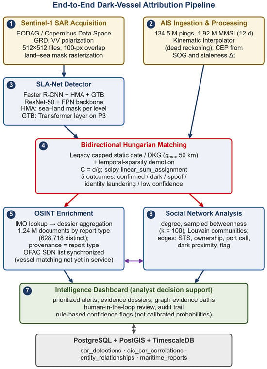
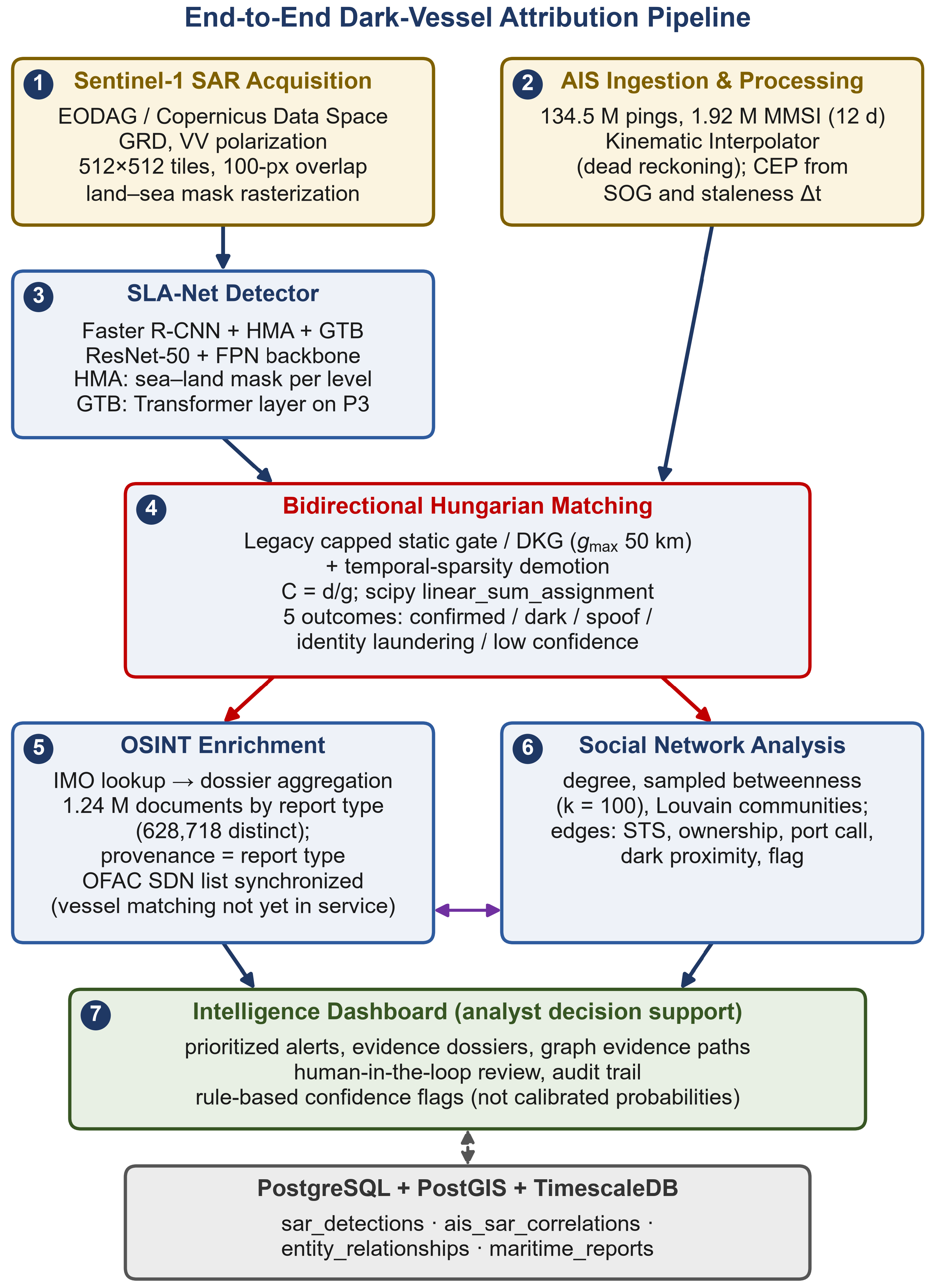
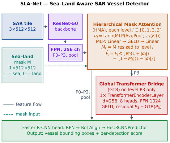
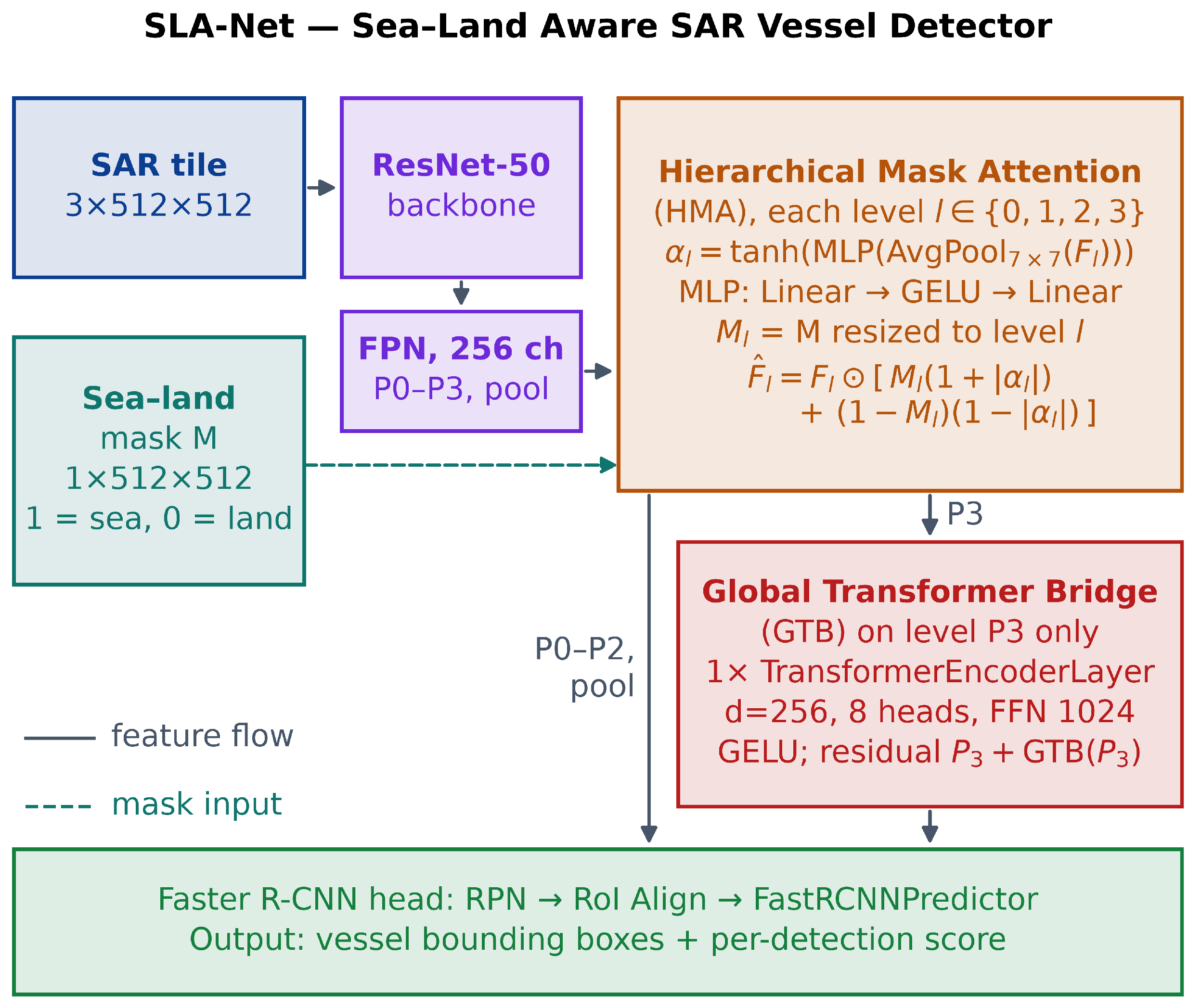
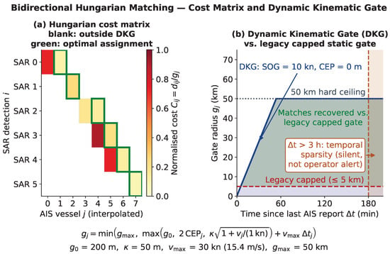
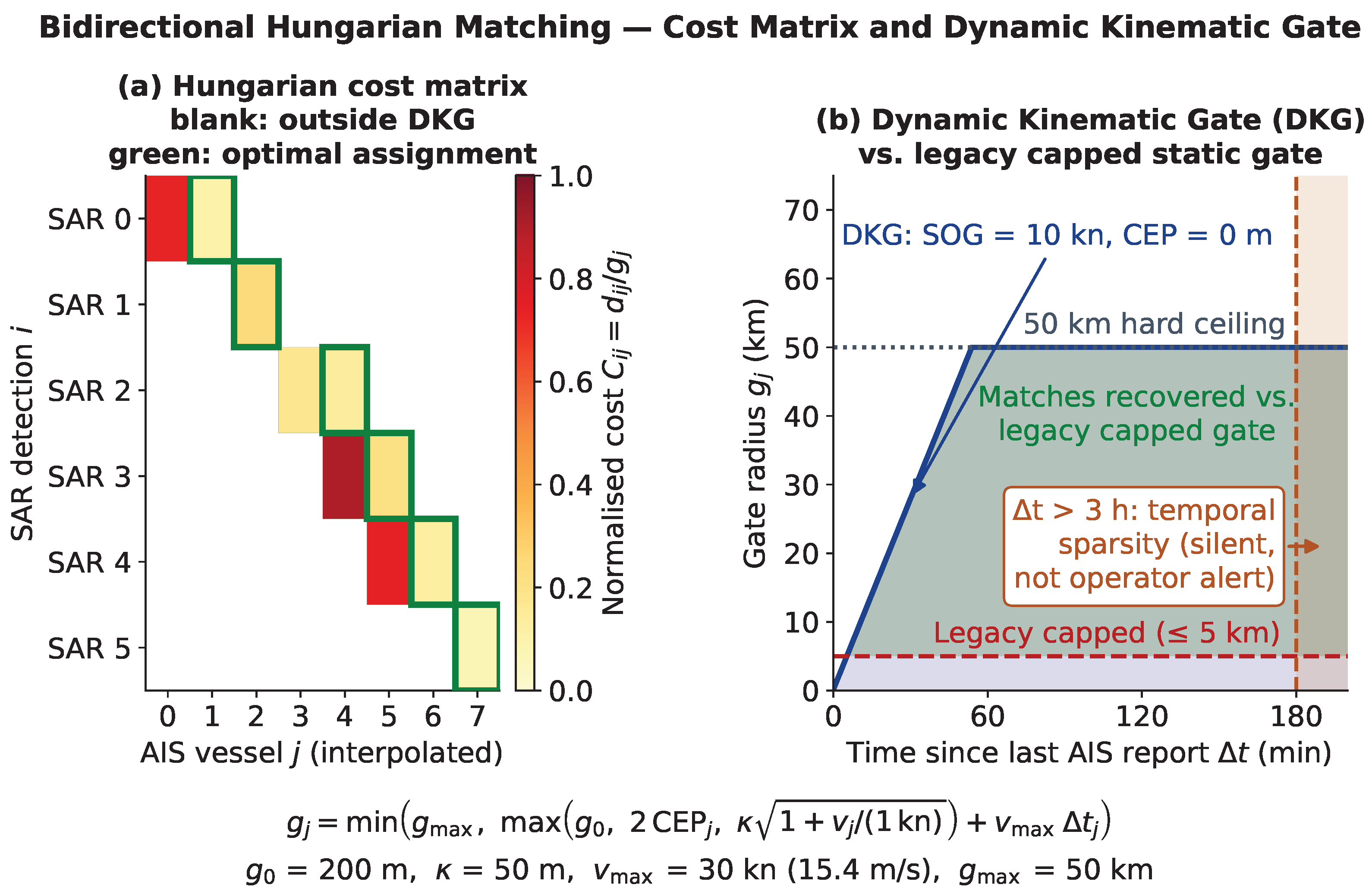
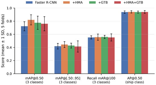
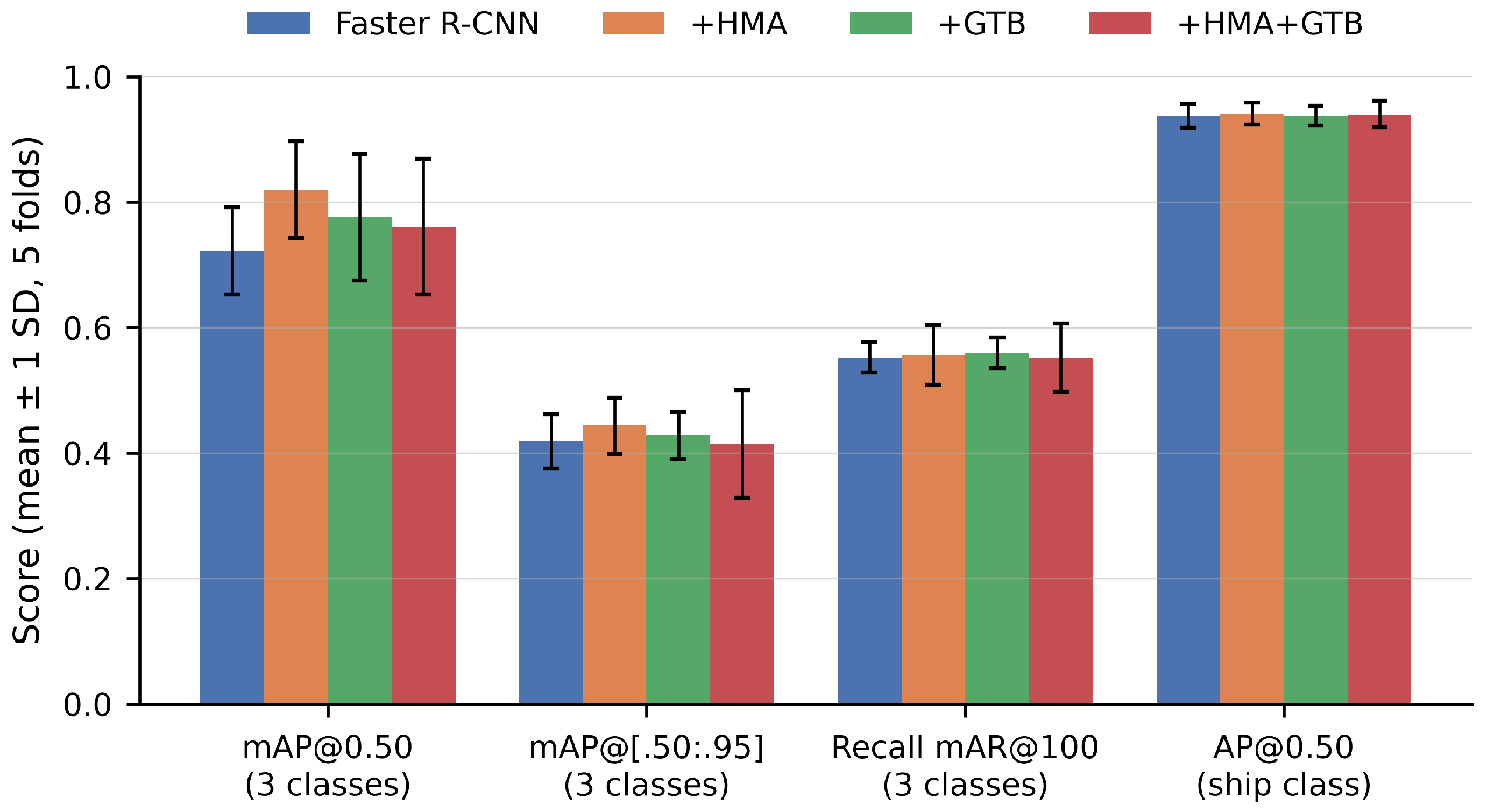
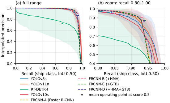
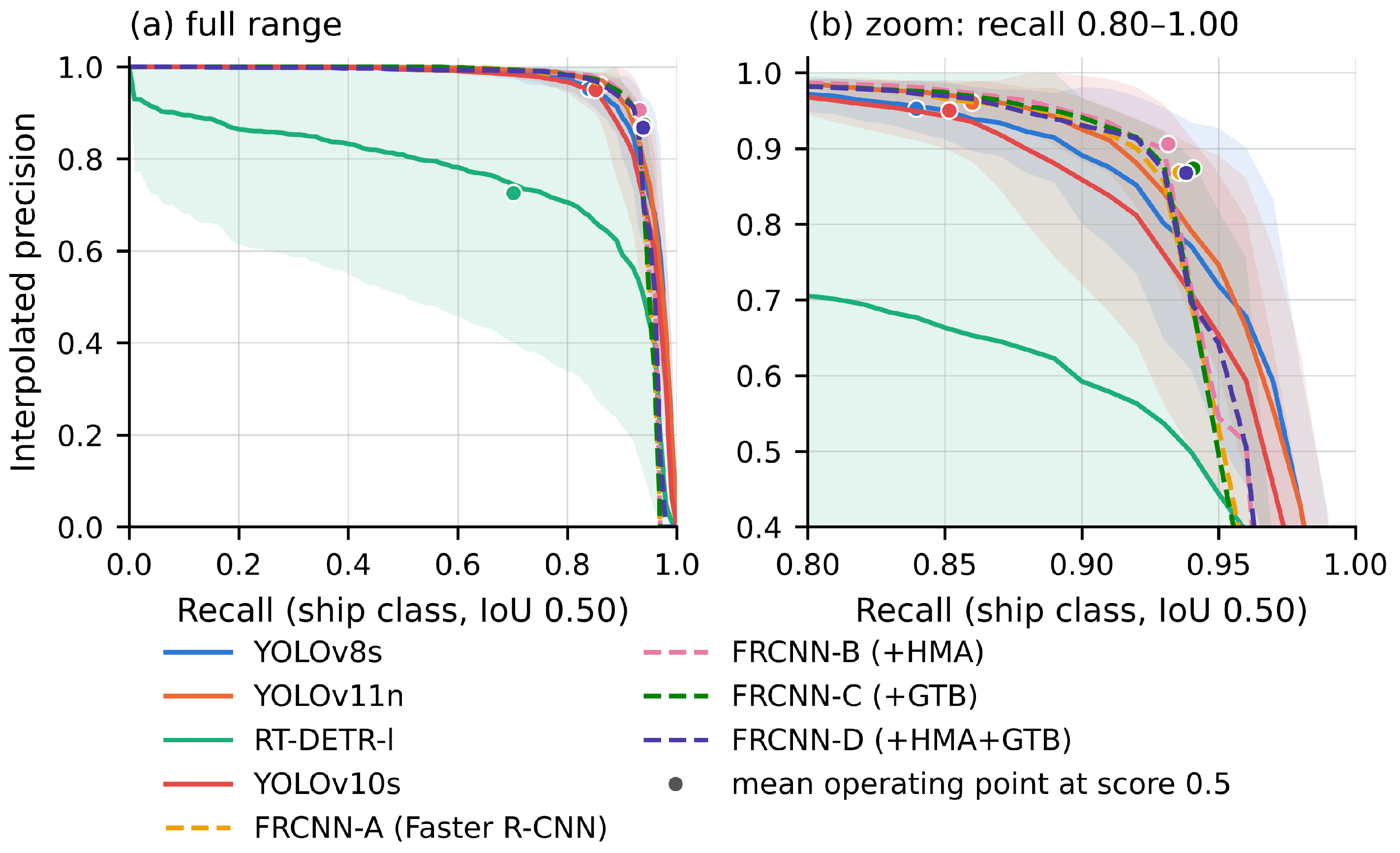
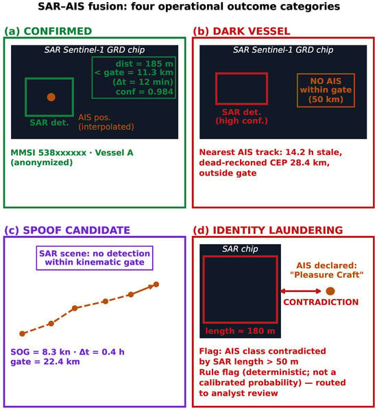
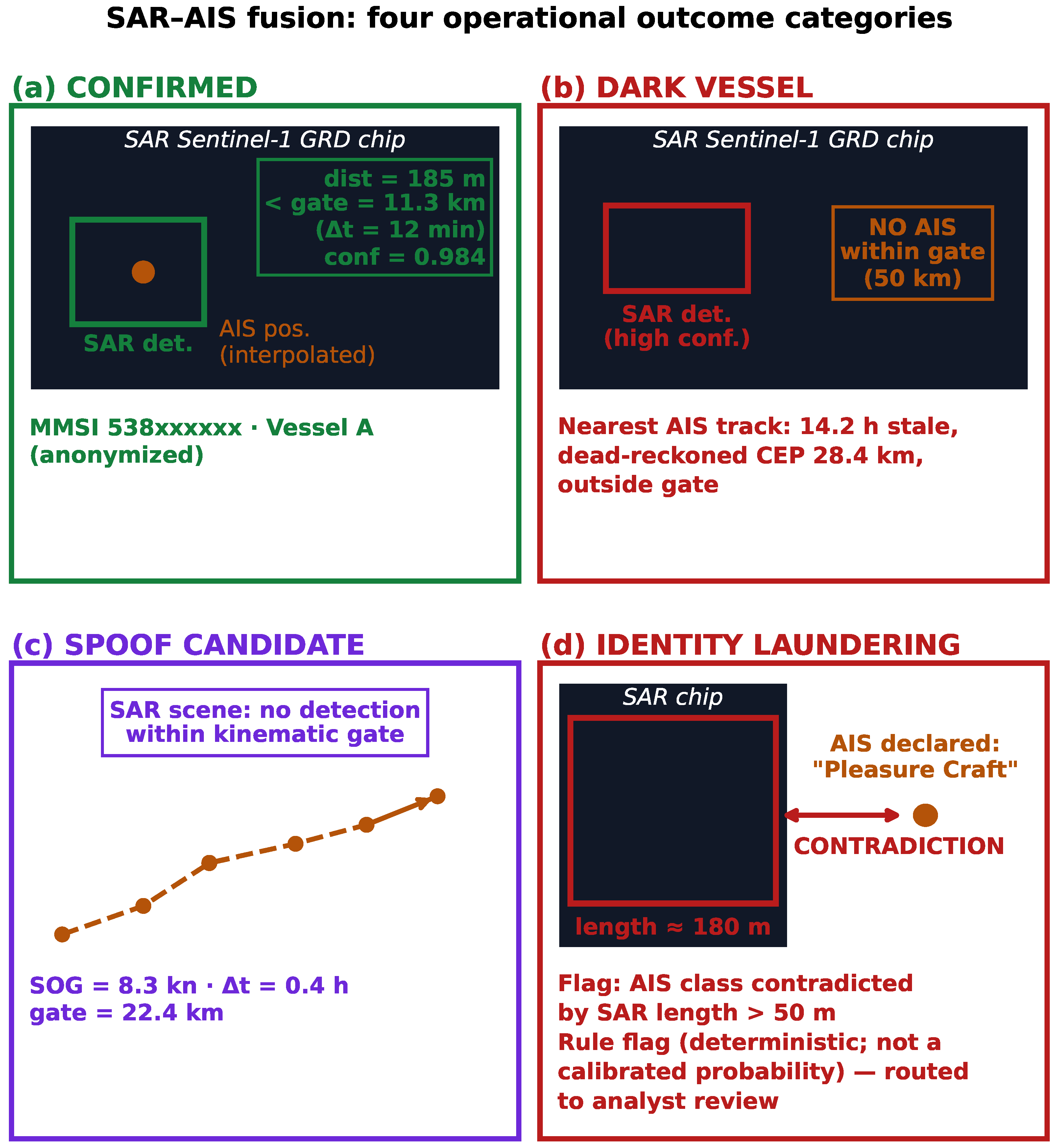
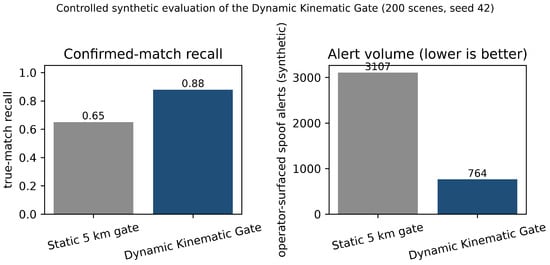
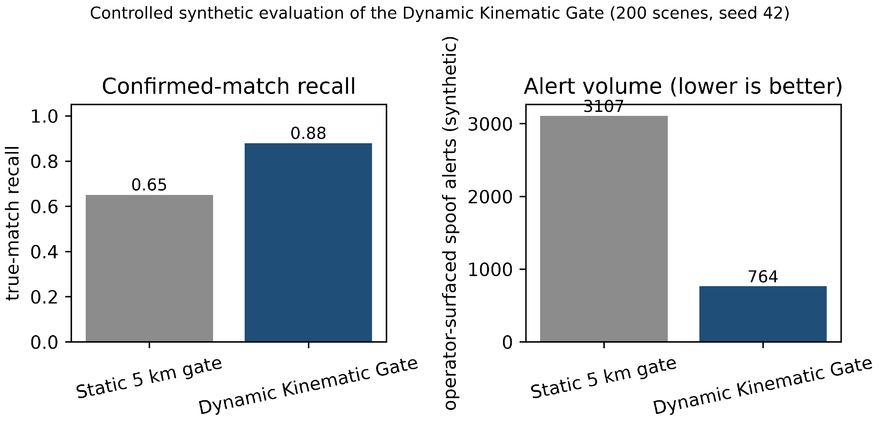
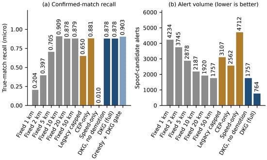
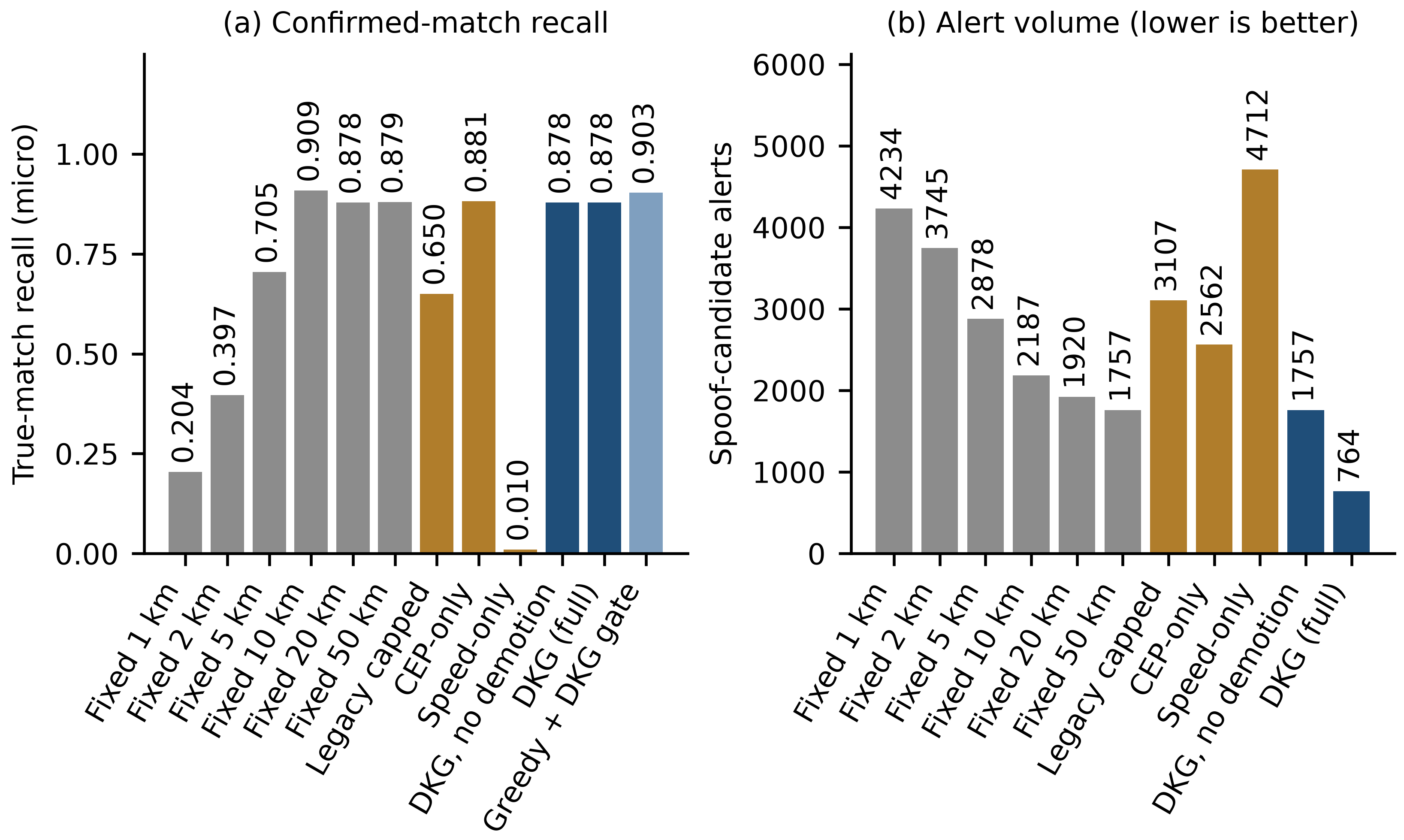
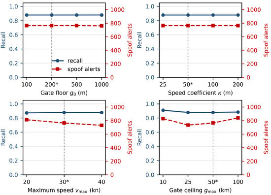
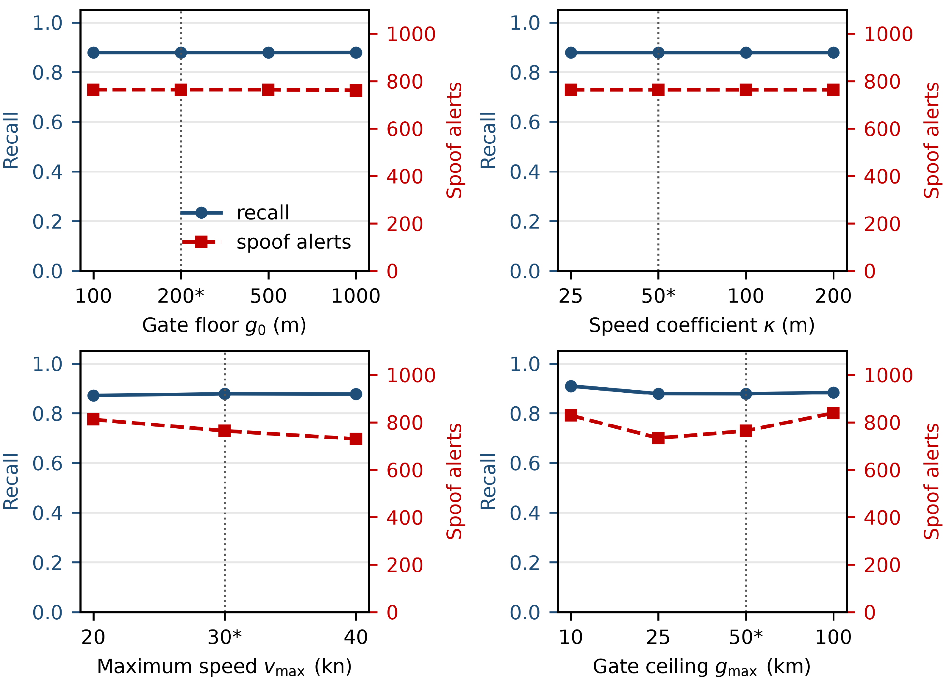
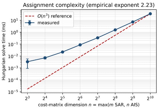
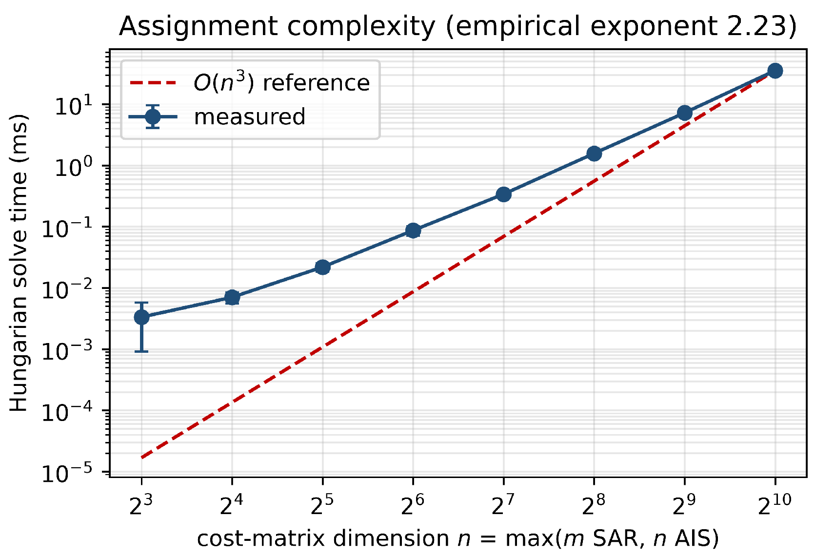
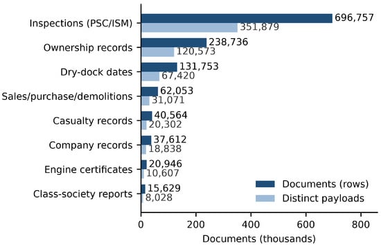
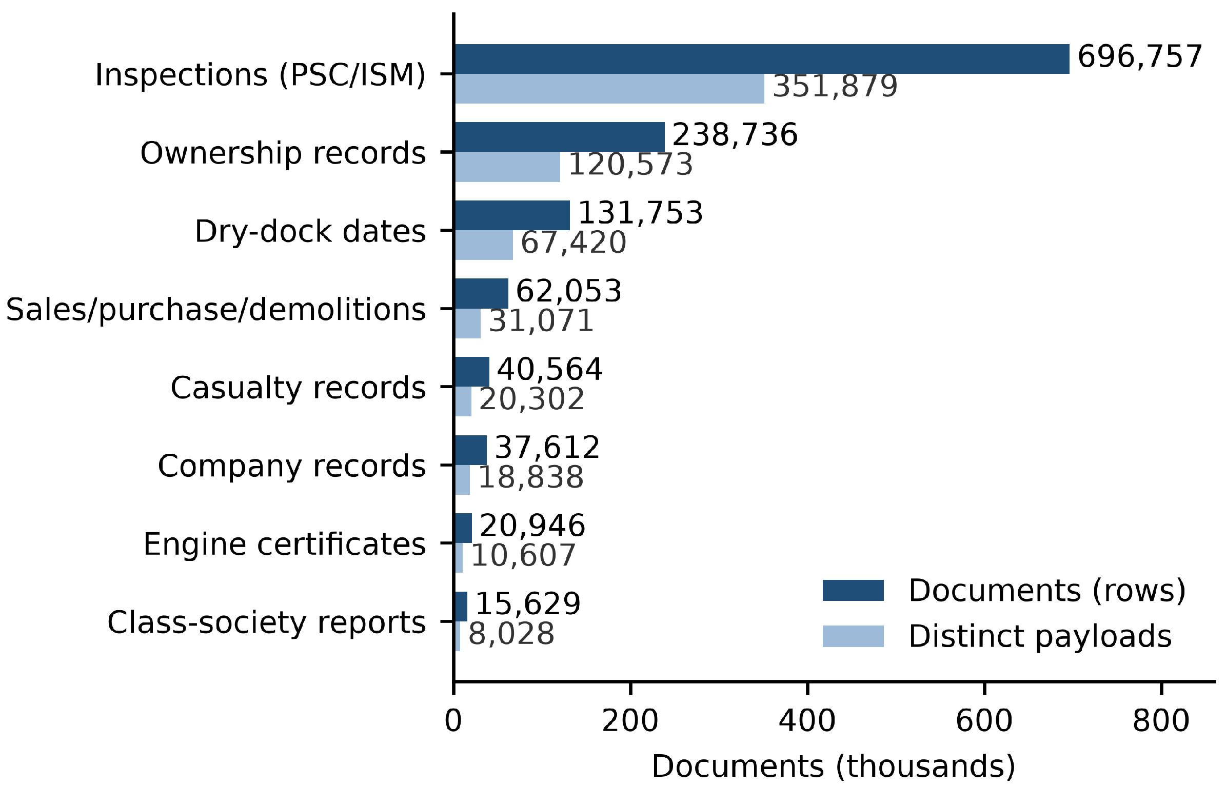
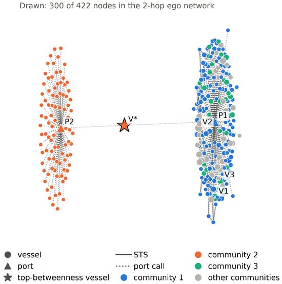
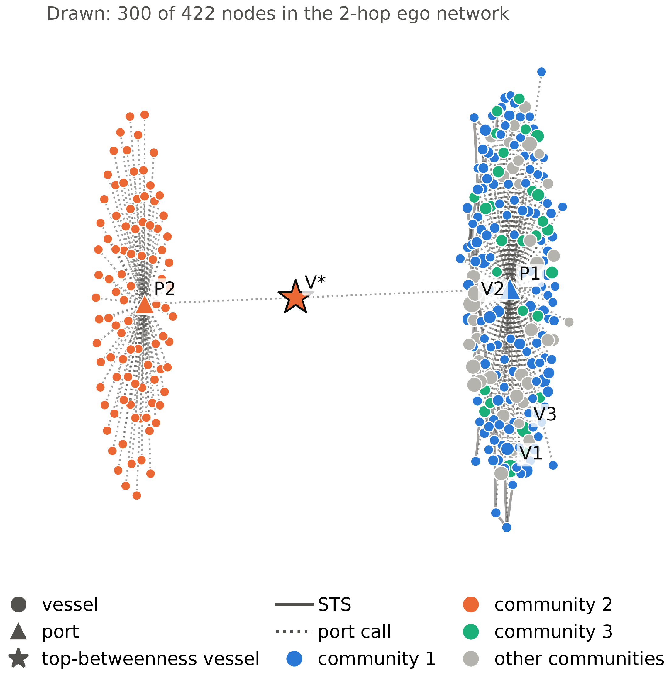
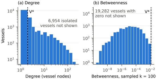
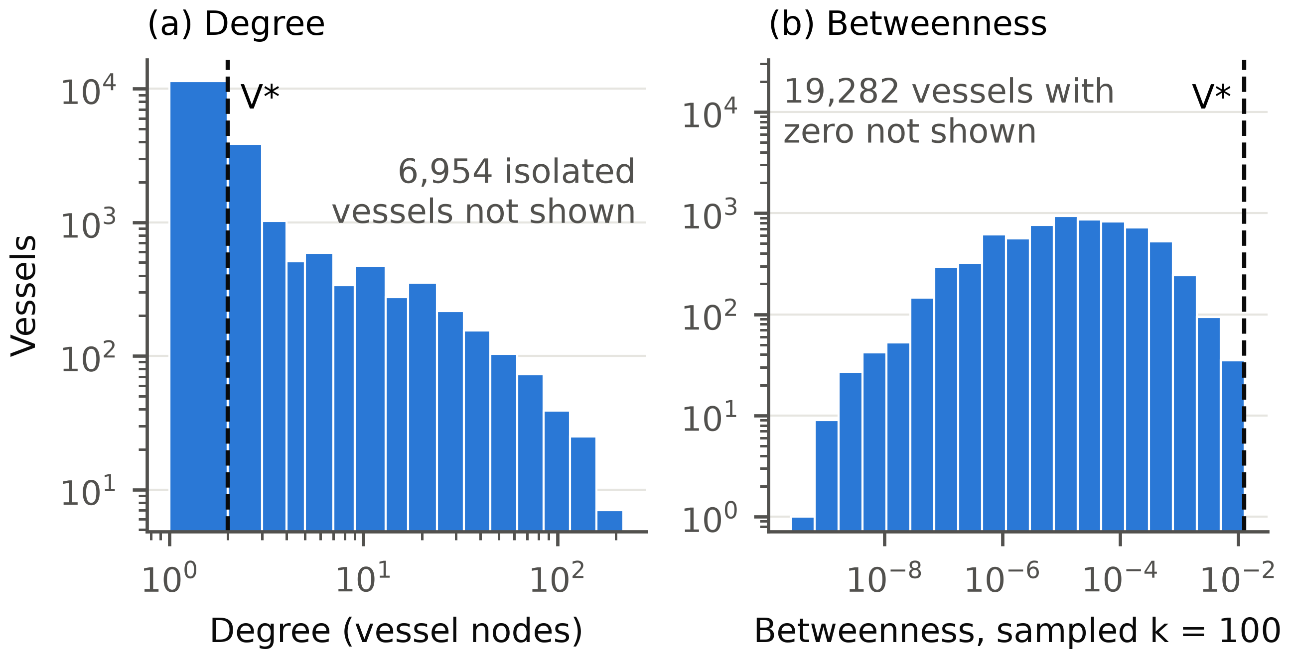
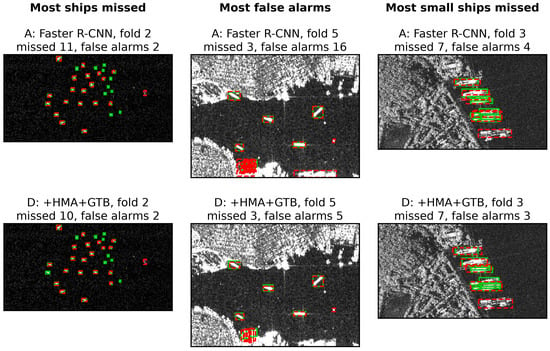
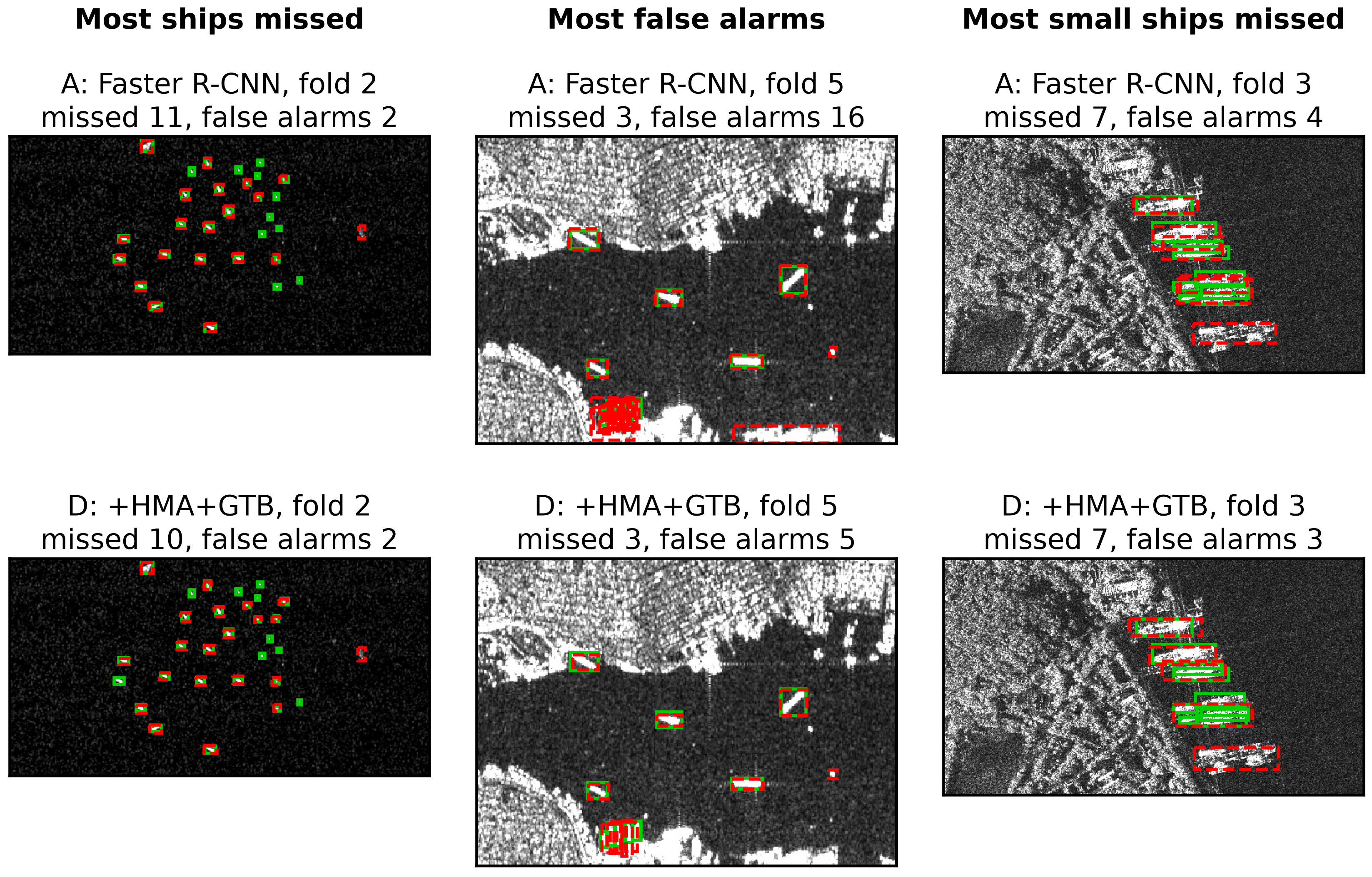
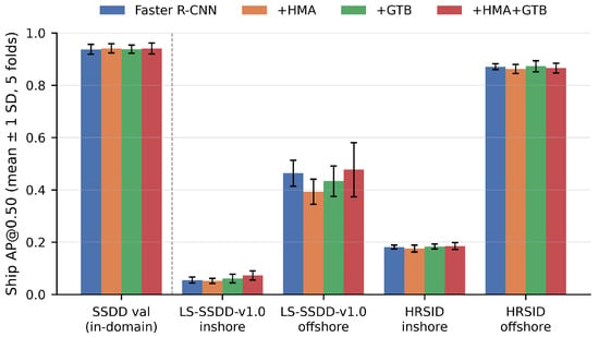
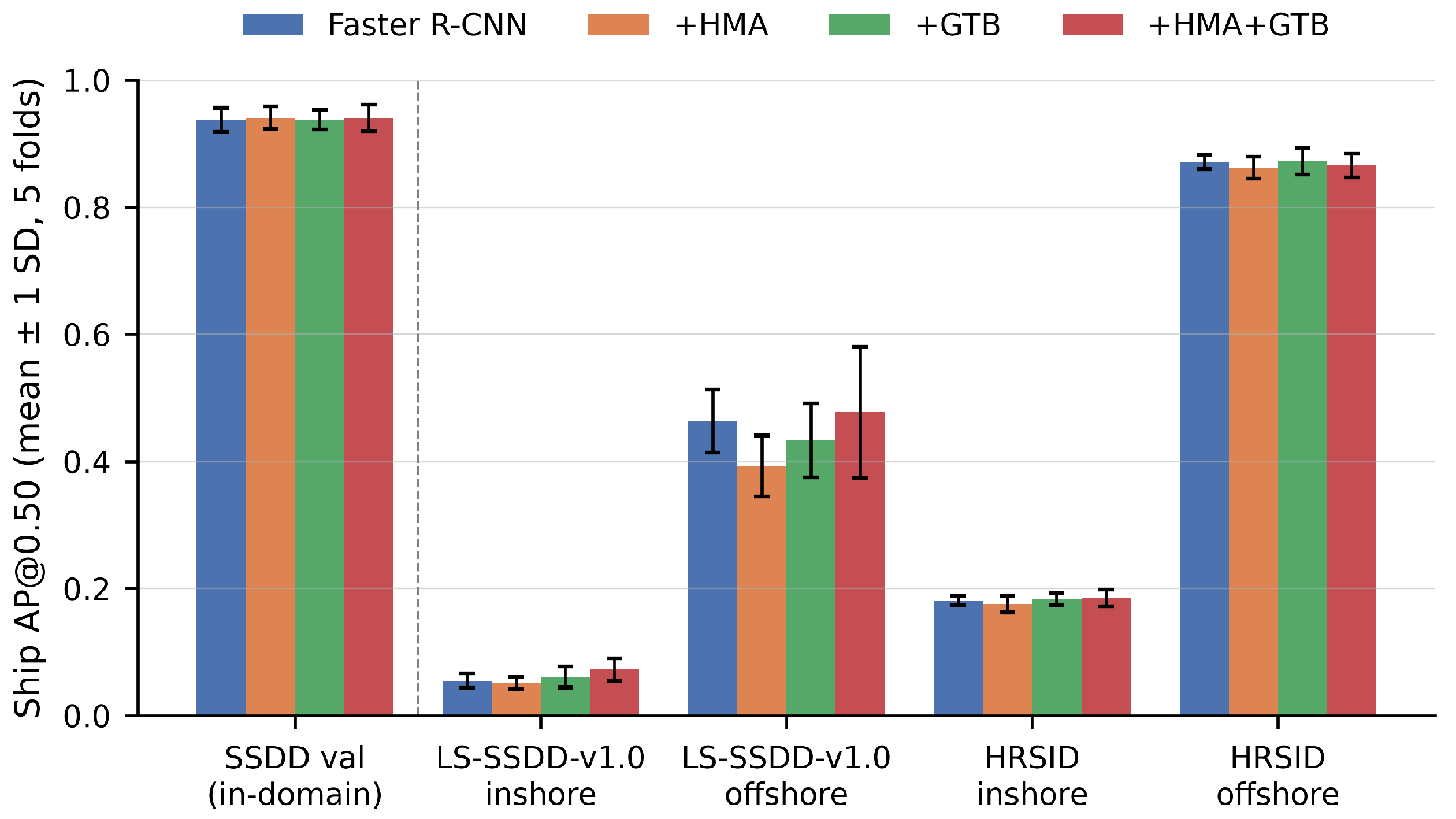

Disclaimer/Publisher’s Note: The statements, opinions and data contained in all publications are solely those of the individual author(s) and contributor(s) and not of MDPI and/or the editor(s). MDPI and/or the editor(s) disclaim responsibility for any injury to people or property resulting from any ideas, methods, instructions or products referred to in the content. |
© 2026 by the authors. Licensee MDPI, Basel, Switzerland. This article is an open access article distributed under the terms and conditions of the Creative Commons Attribution (CC BY) license.