RR-MPF: A Reliable Routing Algorithm Based on Markov Parallel Forecasting for STINs

Abstract

Satellite–Terrestrial Integrated Networks (STINs) undergo frequent topology reconfiguration due to the high mobility of satellite nodes, which can disrupt active routing paths across time slot boundaries, increase packet drop, and degrade end-to-end reliability. This paper proposes RR-MPF (Reliable Routing with Markov Parallel Forecasting), a routing algorithm that selects paths sustaining high reliability across successive time slots. RR-MPF quantifies time-varying link reliability through toughness, delay, jitter, and packet loss metrics. A Markov chain model, executed in a parallel background thread, estimates the probability that each link remains viable in the next time slot, providing future-state awareness without adding online latency. An enhanced Ant Colony Optimization (ACO) then solves a cross-slot weighted optimization that jointly maximizes current and predicted path reliability, yielding path selections that are robust to imminent topology changes. Numerical results show that RR-MPF reduces the average end-to-end delay by up to 23.9%, the delay jitter by 6.4–21.3%, and the packet drop rate by 6.8–34.4%, while improving the overall path reliability by up to 14.0% compared with three benchmark algorithms (iVACO, DPSO-TA, and GA-CG).

1. Introduction

Satellite–Terrestrial Integrated Networks (STINs) are envisioned as a fundamental architecture for ubiquitous interconnection in the next-generation Internet, comprising orbiting satellites, airborne platforms such as unmanned aerial vehicles (UAVs), terrestrial infrastructures, and satellite ground stations, all equipped with computing and storage capabilities. These networks deliver diverse, low-latency, and spectrally efficient wireless communication services [1], and play a pivotal role in telemetry, maritime navigation, intelligence and reconnaissance, and joint operational scenarios [2]. As global communication demands continue to surge, service reliability has become a paramount requirement for such satellite-based information systems.

However, the high mobility of satellite nodes causes frequent and unpredictable topological changes in STINs [3], and communication paths are further challenged by spatiotemporal variations in network scale and channel conditions [4]. These dynamics make it difficult to guarantee deterministic routing quality, particularly when paths must be rescheduled across multiple time slots within the continuously evolving topology [5]. Routing algorithms for STINs must therefore substantially enhance path reliability under such time-varying topological and spatial communication environments [6].

Existing studies on network reliability can be broadly categorized into three research streams.

(1) Network reliability modeling. A rich set of analytical and simulation-based methods has been developed to quantify network reliability, including game-theoretic reliability assessment [7], reliability-bound accumulation [8], Markov processes [9], Petri net modeling [10], fuzzy dynamic Bayesian networks [11], and recursive algorithms for phased-mission systems [12]. Within this stream, generalized artificial neural networks have been applied to estimate the reliability of ring Ethernet networks, yet they struggle to distinguish networks with identical topological inputs [13]. Recursive truncation algorithms (RTAs) compute accurate reliability bounds by scanning all minimum cut sets in the network graph [14]. Dynamic spanning tree methods maximize reliability through strategic edge insertions after comparing spanning tree counts for node pairs [15]. Dynamic fault trees (DFTs) extend static fault tree (SFT) modeling, overcoming the inherent limitations of SFTs in representing performance degradation [16]. A mixed-integer linear programming (MILP) model incorporating max-min fairness establishes upper bounds on reliability during topology mutation periods [17]. All-terminal reliability analysis has been applied to wireless networks of redundant radio modules [18], and network pruning algorithms accelerate K-terminal reliability analysis by eliminating redundant edges and vertices [19]. However, the majority of these methods assume quasi-static topologies and do not account for the rapid, periodic link reconfigurations that characterize STINs.

(2) Reliable routing for satellite and spatial networks. Several studies have targeted reliability-oriented routing specifically in satellite and wireless contexts. Quantitative methods have been developed to evaluate satellite communication network reliability, verifying the ability of adjusted network elements to maintain end-to-end service integrity [20]. The Global and Local Reliability-based Routing (GLRR) protocol ensures reliable source-to-destination data transmission by jointly considering global and local path reliability [21]. Vertex- and edge-disjoint path separation techniques assess connection probability to identify critical non-crossing paths [22]. A path-satisfaction-based reliable routing algorithm has likewise been proposed for the energy internet, selecting paths by matching multi-requirement constraints [23]. In the wireless sensor network (WSN) domain, flow-oriented approaches support multi-state reliability evaluation with enhanced temporal efficiency [24], and reliability evaluation and optimal design methods have been used to improve transmission efficiency [25]. In LEO satellite constellations, a deep-reinforcement-learning routing method with service function constraints has been developed for mega-constellation networks [26], demonstrating the potential of data-driven approaches, although its reliability guarantees under frequent topology changes are less explicit than those of model-based methods. While these methods provide valuable insights, they typically optimize a single reliability metric (e.g., connectivity probability) and do not jointly consider delay, jitter, and packet loss—metrics that are essential for service quality in STINs.

(3) Prediction under time-varying topologies. Markov chain models have been widely adopted to capture state transitions in dynamic networks [9], and reliability-bound updating mechanisms have been proposed to track evolving network states [8]. Nevertheless, existing predictive routing frameworks generally operate in an online fashion, meaning that forecast computation is coupled with—and thus delays—real-time routing decisions. To the best of our knowledge, no prior work has exploited parallel background prediction of link reliability states to enrich cross-slot routing objectives in STINs without introducing additional online latency.

With the proliferation of satellite constellations, ensuring reliable routing has become a critical requirement [6]. Although the aforementioned studies provide valuable foundations, three gaps remain. First, most reliability models assume quasi-static topologies and cannot capture the temporal correlation of link quality across consecutive time slots in STINs. Second, existing reliable routing protocols typically optimize a single metric, failing to integrate multiple time-varying performance indicators into a unified decision framework. Third, existing predictive routing methods couple forecast computation with online path selection, which increases decision latency and is particularly problematic in time-sensitive satellite environments.

To bridge these gaps, we propose RR-MPF, a reliable routing algorithm based on Markov parallel forecasting. The principal contributions of this work are as follows:

• We establish a time-varying multi-metric reliability model for STINs that integrates link toughness, transmission delay, delay jitter, and packet drop rate into a unified quantitative framework. Each metric is normalized using historical statistics and discretized into three reliability levels, enabling consistent cross-metric comparison beyond single-metric evaluation.
• We design a Markov chain-based predictor that estimates the link reliability distribution in the subsequent time slot. The predictor executes in a parallel background thread, decoupling forecast computation from online routing decisions and imposing no additional latency on the data plane.
• We formulate a cross-slot weighted optimization objective that jointly maximizes instantaneous reliability at the current slot and forecasted stability at the next slot, and develop an enhanced Ant Colony Optimization algorithm to solve it, yielding paths that are robust to imminent topological disruptions.
• We conduct extensive simulations under two measured traffic scenarios on an STK and MATLAB-R2026a co-simulation platform with a 24-satellite LEO constellation. RR-MPF reduces the packet drop rate by up to 34.4% and the delay jitter by up to 21.3%, and improves the overall path reliability by up to 14.0% compared with three benchmark algorithms.

The remainder of this paper is organized as follows. Section 2 defines the network model and time-varying link metrics for STINs. Section 3 constructs the Markov chain-based reliability model. Section 4 presents the RR-MPF routing algorithm with its cross-slot optimization objective and ACO-based solver. Section 5 reports the simulation setup and numerical results. Section 6 concludes the paper and discusses future directions.

2. Network Model of the STINs

Temporal network models offer a powerful framework for capturing the time-varying relationships among satellite nodes, thereby facilitating a holistic characterization of both structural and dynamic properties [27]. Unlike terrestrial networks, satellite links in STINs exhibit rapid time-varying characteristics, rendering existing models inadequate for comprehensive network state characterization. To address reliability analysis requirements, this section defines key temporal network parameters, including time-dependent link metrics and time-evolving topology.

In STINs, data flow transmission can be characterized as end-to-end packet forwarding from source to destination nodes via inter-satellite links. The lifespan of the STINs is divided into K time slots, denoted as $\mathcal{K}=\{1,2,\dots ,K\}$, and the physical connectivity within a single time slot remains relatively stable. Let $G_k=⟨V_k^M,E_k^L⟩$ denote the status of the STINs during time slot k, where $V_k^M=\{v_k^1,v_k^2,\dots ,v_k^m\}$ is the set of all nodes, consisting of satellite nodes $S_k=\{s_k^1,s_k^2,\dots ,s_k^a\}$ and ground nodes $g_k=\{g_k^1,g_k^2,\dots ,g_k^b\}$ over the interval $[k,k+1)$. Here, $M=\{1,2,\dots ,m\}$ is the node index set and $m=a+b$ is the total number of satellite and ground nodes. $E_k^L$ denotes the set of transmission links available in time slot k, and L is the total number of potential links.

2.1. Toughness of a Link

Definition 1 

(Link Toughness). The toughness of a link $e_k^{v^i,v^j}$ measures its ability to maintain reliable transmission over consecutive time slots. It is defined as the normalized expected service capability in the next time slot $k+1$.

Let $B_{max}$ denote the nominal maximum capacity of the link. In time slot k, the remaining service capability $s{c}_k^{v^i,v^j}$ is normalized to a dimensionless factor:

$${\widehat{sc}}_k^{v^i,v^j}={\displaystyle \frac{s{c}_k^{v^i,v^j}}{B_{max}}}\in [0,1].$$

(1)

Let $P_{k+1}^e$ be the probability that the link becomes unavailable in the next slot (e.g., because node movement exceeds the line of sight). Then the toughness $H_{e_k}^{v^i,v^j}$ is the expected normalized capacity available in the upcoming slot:

$$H_{e_k}^{v^i,v^j}=\left(1-P_{k+1}^e\right)·{\widehat{sc}}_k^{v^i,v^j}.$$

(2)

A higher toughness value indicates stronger resilience in maintaining effective service continuity, thereby improving overall path reliability under time-varying topologies.

2.2. Average Link Delay

The end-to-end packet delay from source to destination node during time slot k comprises four components: propagation delay $D_{PP}$, transmission delay $D_{TR}$, queuing delay $D_{QU}$, and processing delay $D_{PC}$. Among these, the propagation delay and the queuing delay are primarily dependent on the current link connection and the node buffer occupancy. Since variations in $D_{PP}$ and $D_{QU}$ significantly impact network reliability, they serve as direct performance indicators for reliability quantification [28].

Definition 2. 

The propagation delay is the time required for traffic flow $x_i$ to traverse the physical distance from source node $v^i$ to destination node $v^j$ along the selected routing path.

Consider a traffic flow $x_i$ routed along the path $\mathrm{path}\left(x_i\right)=\{v^i,v^{i+1},\dots ,v^{i+j\left(x_i\right)}\}$, where $j\left(x_i\right)$ denotes the number of hops. The change in transmission distance caused by node movement within time slot k can be computed from the node position coordinates.

The average end-to-end propagation delay of traffic flow $x_i$ in time slot k is defined in Equation (3).

$$D_k^{pp}={\displaystyle \frac{1}{N}}{\displaystyle \sum _{i=1}^{j\left(x_i\right)}}{\displaystyle \sum _{n=1}^N}{\displaystyle \frac{l_n^{v^i,v^{i+1}}}{c}}.$$

(3)

$l_n^{v^i,v^{i+1}}$ denotes the link length between node $v^i$ and $v^{i+1}$ at the n-th sub-interval of slot k, N is the number of sub-intervals into which the slot is divided (consistent with the jitter definition in Section 2.3), and c is the propagation speed of electromagnetic waves. Each term $l_n/c$ is a propagation time, so the double sum divided by N yields the average propagation delay over the sub-intervals and hops. The link length $l_n^{v^i,v^{i+1}}=∥{\mathbf{r}}^{v^i}\left(t_n\right)-{\mathbf{r}}^{v^{i+1}}\left(t_n\right)∥$ is computed as the Euclidean distance between the two node positions, where $t_n$ is the midpoint of the n-th sub-interval.

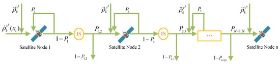
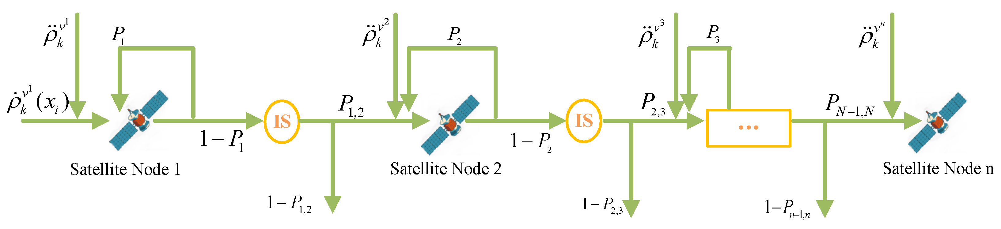
Queueing models provide an accurate representation of the multi-hop transmission structure in communication systems. Within STINs, each node is modeled as an $M/M/h/R$ system, where h denotes the number of processing queues and R the shared buffer capacity; the $M/M/1/R$ formulation corresponds to the single-queue special case. The end-to-end routing path is thus abstracted as a tandem queueing network, as illustrated in Figure 1.

Figure 1. Tandem queue model of a multi-hop routing path.

In Figure 1, ${\dot{\rho }}_k^{v^i}\left(x_i\right)$ denotes the average arrival rate of node $v^i$ for traffic flow $x_i$ in time slot k, which follows the Pareto distribution. Similarly, ${\ddot{\rho }}_k^{v^i}$ represents the average arrival rate of other traffic received by node $v^i$ in time slot k. Assuming the node adopts a TDMA multiplexing scheme, $P_i$ denotes the probability that node $v^i$ must wait for a time slot, while $1-P_i$ indicates the probability of successful data transmission at node $v^i$. $P_{i,i+1}$ represents the probability of data entering the next node, and $1-P_{i,i+1}$ gives the probability of data leaving the node.

Based on the above network queuing model, the average arrival rate ${\rho }^{v^i}$ of node $v^i$ in time slot k is defined in Equation (4).

$$\begin{array}{c}{\rho }^{v^1}=\left({\dot{\rho }}^{v^1}\left(x_i\right)+{\ddot{\rho }}^{v^1}\left(x_i\right)\right)\left(1+P_1\right).\hfill \\ {\rho }^{v^2}=\left({\rho }^{v^1}\left(x_i\right)\left(1-P_1\right)P_{1,2}+{\ddot{\rho }}^{v^2}\left(x_i\right)\right)\left(1+P_2\right).\hfill \\ {\rho }^{v^3}=\left({\rho }^{v^2}\left(x_i\right)\left(1-P_2\right)P_{2,3}+{\ddot{\rho }}^{v^3}\left(x_i\right)\right)\left(1+P_3\right).\hfill \\ ⋮\hfill \\ {\rho }^{v^n}=\left({\rho }^{v^{n-1}}\left(x_i\right)\left(1-P_{n-1}\right)P_{n-1,n}+{\ddot{\rho }}^{v^{\mathrm{n}}}\left(x_i\right)\right)\left(1+P_n\right).\hfill \end{array}$$

(4)

${\rho }^{v^i}$ comprises three components: the arrival rate ${\dot{\rho }}^{v^i}\left(x_i\right)$ of traffic flow $x_i$, the arrival rate ${\ddot{\rho }}^{v^i}$ of other traffic, and the probability $P_i$ of transmission failure or retransmission.

Lemma 1. 

For an $M/M/h/R$ queue at node $v^i$ (the $M/M/1/R$ case being the single-queue special case) with arrival rate ${\rho }_k^{v^i}$ and service rate ${\mu }^{v^i}$, the steady-state average queue waiting time is given by $W_q^{v^i}=L_q^{v^i}/({\rho }_k^{v^i}·(1-{\lambda }_0))$, where $L_q^{v^i}$ is the average queue length and ${\lambda }_0$ is the idle probability, both derived in Appendix A [29].

By the delay additivity principle, Equation (5) defines the average end-to-end queuing delay for traffic flow $x_i$.

$$D_k^{qu}={\displaystyle \sum _{i=1}^{j\left(x_i\right)}}{W}_q^{v^i}.$$

(5)

The total end-to-end time delay of the routing path for traffic flow $x_i$ in time slot k is defined in Equation (6).

$$D_k^{v^i,v^j}=D_k^{pp}+D_k^{qu}+D_k^{tr}+D_k^{pc}.$$

(6)

The Pareto traffic model generates bursty ON/OFF load, while the Markovian $M/M/h/R$ queueing model serves as a first-order analytical approximation of buffer behavior for reliability computation. All performance results in Section 5 are obtained from discrete-event simulations rather than from this analytical model.

Queueing memory across time slots is captured by a per-link congestion backlog. When the realized peak utilization of a link exceeds the congestion-detection threshold (the same signal that drives the Markov telemetry rule), residual backlog accumulates in proportion to the degree of overload and then drains geometrically at the finite service rate in subsequent slots. Each unit of backlog contributes up to one full-buffer stationary waiting time to the queueing term $W_q$. Therefore, sustained congestion causes the end-to-end delay to grow cumulatively, and this increase persists after the traffic burst subsides, whereas packet loss remains governed by the per-slot stationary blocking probability.

2.3. Link Delay Jitter

Definition 3 

(Delay Jitter). The delay jitter $J_k$ quantifies the variability of the end-to-end delay around its mean over a specified observation interval. Formally, it is defined as the variance of the delay under stochastic disturbances: $J_k=\mathbb{E}\left[|D_k-{\overline{D}}_k{|}^2\right]$.

Consider the link from node $v^i$ to node $v^j$. The average delay ${\overline{D}}_k$ during time slot k is computed via Equation (6). Each time slot has a fixed duration $\Delta t$ and is divided into N equal sub-intervals, so each sub-interval has length $\Delta t/N$. Let $D_n^{v^i,v^j}$ denote the average delay from $v^i$ to $v^j$ measured over the n-th sub-interval, where $n=1,2,\dots ,N$. Then the link delay jitter $J_k^{v^i,v^j}$ is defined as the mean squared deviation from ${\overline{D}}_k$:

$$J_k^{v^i,v^j}={\displaystyle \frac{1}{N}}{\displaystyle \sum _{n=1}^N}{\left|D_n^{v^i,v^j}-{\overline{D}}_k\right|}^2.$$

(7)

2.4. Average Packet Drop Rate

Packet drop in STINs is defined as the failure to transmit packets during service delivery.

Definition 4. 

Consider a traffic flow $x_i$ routed along the path $path\left(x_i\right)=\{v^i,\dots ,v^{i+w\left(x_i\right)}\}$, where $w\left(x_i\right)$ denotes the hop count. For each constituent link $e_k^{v^i,v^{i+1}}$ connecting node $v^i$ to $v^{i+1}$ during time slot k, the average packet drop rate $O_k^{v^i,v^{i+1}}$ is defined as the ratio of lost packets to total packets sent, as expressed in (8).

$$O_k^{v^i,v^{i+1}}={\displaystyle \frac{n_{drop}(v^i,v^{i+1})}{n_{total}(v^i,v^{i+1})}}.$$

(8)

Assuming independent packet drops on each link, the end-to-end packet drop rate along the path is given by the cascade formula (9).

$$O_k^{v^i,v^j}=1-\prod _{i,j\in \{1,2,\cdots ,w\left(x_i\right)\}}\left(1-O_k^{v^i,v^{i+1}}\right).$$

(9)

3. Link Reliability Modeling Based on Markov Chains

The reliability state of an STIN link fluctuates due to frequent topology changes and localized traffic bursts. The Markov chain framework is well suited for capturing such state transitions, as it exhibits the memoryless property: the state at time k depends only on the state at the immediately preceding time $k-1$ [30].

3.1. Performance Parameter Processing

Ensuring high reliability and low variability in communication networks during service transmission is critical. Although researchers have proposed diverse metrics for complex network reliability, evaluation systems and standards remain inconsistent. To comprehensively assess path reliability in STINs, this section adopts link survivability and performance indicators as measurement criteria.

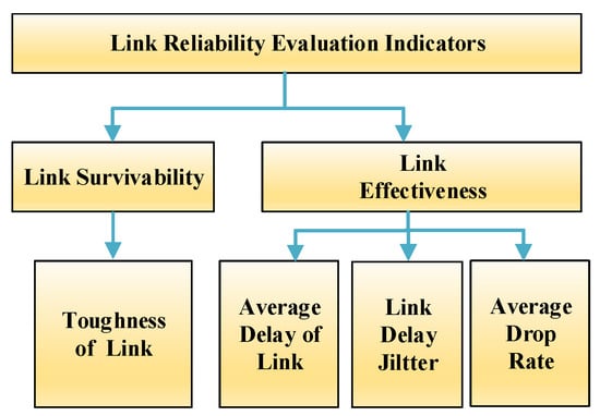
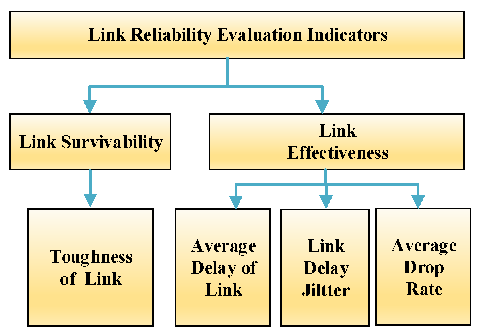
Link survivability represents the ability to maintain an acceptable communication state when network node failures occur or links move beyond line of sight. A higher probability of maintaining link stability corresponds to stronger link reliability. The link performance indicators include average service delay, delay jitter, average link packet loss rate, and related metrics. The time is divided into equal intervals, with aggregated performance metrics per network iteration cycle representing routing result states during system operation. The evaluation indicators for STIN link reliability are shown in Figure 2.

Figure 2. Reliability evaluation indicators of the STINs.

Frequent topology changes caused by routing switching and delay jitter in satellite ground network connections significantly impact communication effectiveness and substantially reduce network reliability. To satisfy the computational requirements of performance parameters in the satellite network, the following performance parameters are selected and normalized.

Let $M=4$ denote the number of performance indicators. Define the performance parameter vector for the multi-hop path from node $v^i$ to node $v^j$ in time slot k as $X_{v^i,v^j}^k=(X_{v^i,v^j}^k\left[1\right],X_{v^i,v^j}^k\left[2\right],\cdots ,X_{v^i,v^j}^k\left[M\right])$, where $X_{v^i,v^j}^k\left[1\right]=H$ (link toughness, Equation (2)), $X_{v^i,v^j}^k\left[2\right]=D$ (average traffic delay, Equation (6)), $X_{v^i,v^j}^k\left[3\right]=J$ (delay jitter, Equation (7)), and $X_{v^i,v^j}^k\left[4\right]=P$ (packet drop rate, Equation (9)).

The reliability evaluation performance of the STINs is determined by the $M=4$ indicators mentioned above, each of which affects system reliability. To meet the $[0,1]$ range required by the subsequent aggregation and quantization, we normalize each indicator using a direction-aware min-max mapping over the historical observation window $\{1,2,\dots ,k-1\}$. For the benefit-type metric (link toughness, $n=1$), larger raw values are better, whereas for the cost-type metrics (delay, jitter, packet drop rate, $n=2,3,4$), smaller raw values are better; therefore, the cost-type metrics are reversed during normalization. Denoting the historical minimum and maximum of metric n over the window by $X_{min}\left[n\right]$ and $X_{max}\left[n\right]$, the normalized value ${\hat{X}}_{v^i,v^j}^k\left[n\right]$ is defined in Equation (10).    

$${\hat{X}}_{v^i,v^j}^k\left[n\right]=\left\{\begin{array}{cc}{\displaystyle \frac{X_{v^i,v^j}^k\left[n\right]-X_{min}\left[n\right]}{X_{max}\left[n\right]-X_{min}\left[n\right]}},\hfill & n=1\left(\mathrm{benefit}\text{-}\mathrm{type}\right),\hfill \\ {\displaystyle \frac{X_{max}\left[n\right]-X_{v^i,v^j}^k\left[n\right]}{X_{max}\left[n\right]-X_{min}\left[n\right]}},\hfill & n=2,3,4\left(\mathrm{cost}\text{-}\mathrm{type}\right).\hfill \end{array}\right.$$

(10)

Consequently, every normalized metric lies in $[0,1]$, and larger values always indicate higher reliability regardless of the metric direction. As a numerical safeguard, in the degenerate case of a zero observed range ($X_{max}\left[n\right]=X_{min}\left[n\right]$, i.e., a metric with no variation over the window), the normalized value is set to 1 for the benefit-type metric and to $0.5$ for the cost-type metrics, thereby avoiding division by zero. For computational convenience, the processed normalized reliability attributes are denoted as in Equation (11).

$$\hat{X}=\{\hat{X}\left[1\right],\hat{X}\left[2\right],\dots ,\hat{X}\left[M\right]\}.$$

(11)

3.2. Markov Chain Construction

The state space of the DTMC is defined consistently throughout this paper: the aggregated link reliability value $r\in [0,1]$ (constructed in Equation (12)) is quantized into three states, $s_1\in [0.80,1]$, $s_2\in [0.40,0.80)$, and $s_3\in [0,0.40)$. These three states are used consistently for the Markov model in this section and for the reliability-level definitions in Section 5. The sensitivity of the routing behavior to the two thresholds is examined in the sensitivity analysis of Section 5.

For brevity, we denote the standardized metrics as ${\hat{H}}_k^{v^i,v^j}={\hat{X}}_{v^i,v^j}^k\left[1\right]$, ${\hat{D}}_k^{v^i,v^j}={\hat{X}}_{v^i,v^j}^k\left[2\right]$, ${\hat{J}}_k^{v^i,v^j}={\hat{X}}_{v^i,v^j}^k\left[3\right]$, and ${\hat{P}}_k^{v^i,v^j}={\hat{X}}_{v^i,v^j}^k\left[4\right]$.

To obtain a tractable scalar metric for reliability assessment, we aggregate the four standardized indicators into a single comprehensive reliability value. The reliability of link $e_k^{v^i,v^j}$ in time slot k is defined as the weighted sum of its normalized metrics:

$$R_k^{v^i,v^j}=\vartheta ·{\left[{\hat{H}}_k^{v^i,v^j},{\hat{D}}_k^{v^i,v^j},{\hat{J}}_k^{v^i,v^j},{\hat{P}}_k^{v^i,v^j}\right]}^T=r,$$

(12)

where the weight vector $\vartheta =[{\vartheta }_1,{\vartheta }_2,{\vartheta }_3,{\vartheta }_4]$ satisfies ${\sum }_{n=1}^4{\vartheta }_n=1$. In this work, an equal-weight strategy is adopted with ${\vartheta }_n=0.25$, which provides a balanced evaluation without subjective bias; alternative weighting schemes (e.g., entropy-based or service-specific) can also be adopted when needed. Because larger normalized values always indicate higher reliability for all four indicators (Section 3.1), the aggregation in Equation (12) is monotonically increasing in path reliability.

The continuous reliability value $r\in [0,1]$ is then quantized into three discrete levels $\mathcal{S}=\{s_1,s_2,s_3\}$, defined as $s_1$ for $[0.80,1.0]$, $s_2$ for $[0.40,0.80)$, and $s_3$ for $[0.0,0.40)$. These three levels constitute the state space of the discrete-time Markov chain (DTMC) introduced below, and are used consistently for the Markov model and the reliability-level definitions in Section 5.

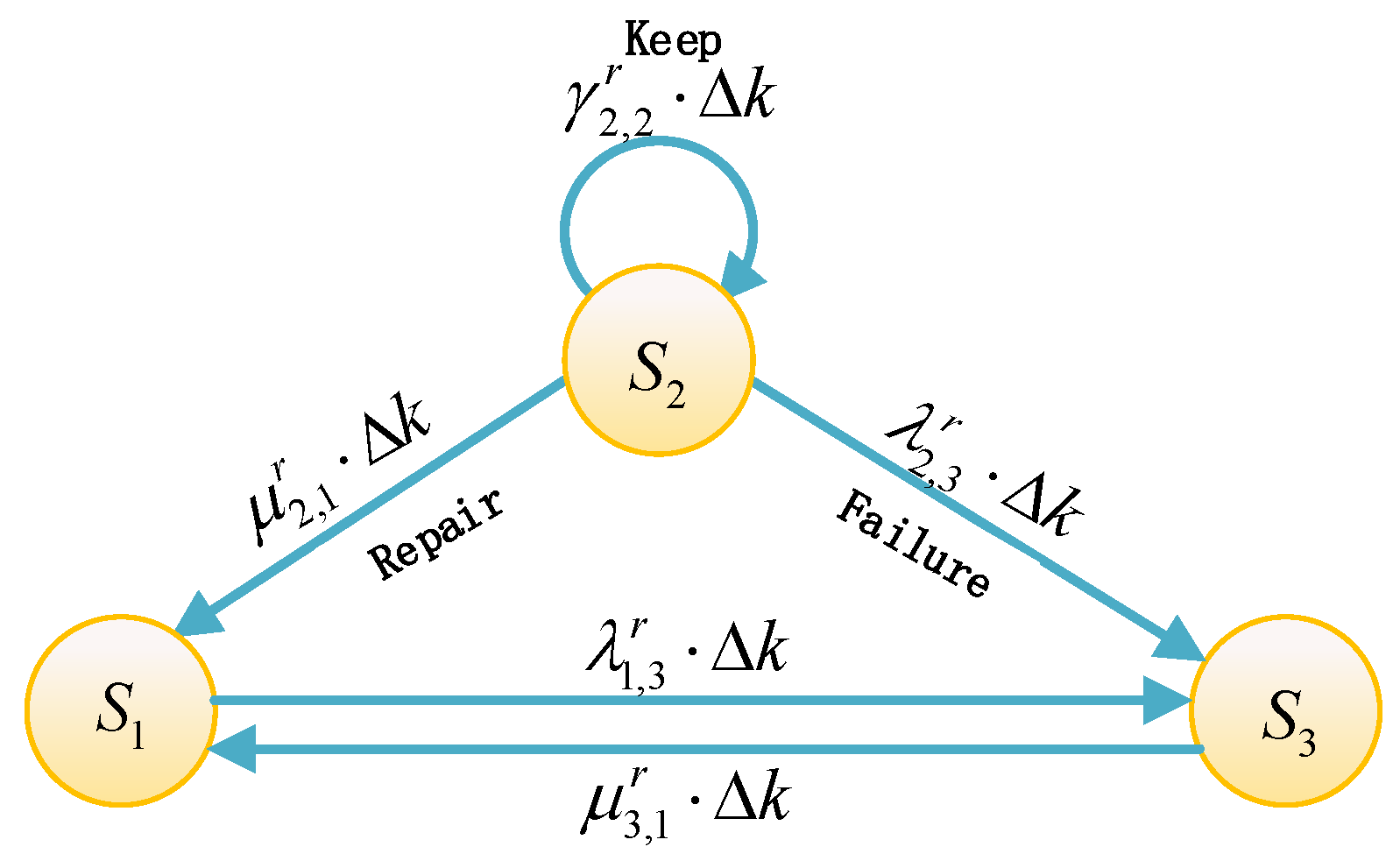
Since the STINs’ topology and traffic conditions are observed at discrete time slot boundaries, we model the evolution of the link reliability state as a DTMC. Let the state of link $e_k^{v^i,v^j}$ at slot k be $s\left(k\right)\in \mathcal{S}$. The state transition probability from state $s_i$ to state $s_j$ during one time slot is denoted by

$$P_{ij}^r=Pr\left(s(k+1)=s_j\mid s\left(k\right)=s_i\right),i,j\in \{1,2,3\}.$$

(13)

These probabilities constitute the transition matrix ${\mathbf{P}}^r={\left[P_{ij}^r\right]}_{3\times 3}$, which satisfies ${\sum }_{j=1}^3{P}_{ij}^r=1$ for all i. The state transition process is illustrated in Figure 3.

Figure 3. Markov state transition among the three reliability levels.

Given the initial state distribution $\mathit{\pi }\left(0\right)=[{\pi }_1\left(0\right),{\pi }_2\left(0\right),{\pi }_3\left(0\right)]$, where ${\pi }_i\left(0\right)=Pr(s\left(0\right)=s_i)$, the state probability vector at time slot k is obtained via the Chapman–Kolmogorov equation:

$$\mathit{\pi }\left(k\right)=\mathit{\pi }\left(0\right)·{\left({\mathbf{P}}^r\right)}^k,$$

(14)

where $\mathit{\pi }\left(k\right)=[p_{s_1}^r\left(k\right),p_{s_2}^r\left(k\right),p_{s_3}^r\left(k\right)]$ denotes the probability distribution over the three states at slot k.

The entries of ${\mathbf{P}}^r$ are estimated online from the historical state transitions observed during network operation. Specifically, let $n_{ij}$ be the number of times a link transitions from state $s_i$ to $s_j$ in consecutive slots over a sliding window of W past slots. The transition probability is then estimated via maximum likelihood as

$${\hat{P}}_{ij}^r={\displaystyle \frac{n_{ij}}{{\sum }_{j=1}^3{n}_{ij}}},$$

(15)

with Laplace smoothing applied to handle unseen transitions. As the network evolves, the transition matrix is updated periodically to adapt to changing dynamics.

For forecasting the state distribution in the next time slot $\Gamma =k+1$, we directly use the one-step transition:

$$\mathit{\pi }(k+1)=\mathit{\pi }\left(k\right)·{\mathbf{P}}^r.$$

(16)

This prediction is computed in a parallel background thread and imposes no additional latency on routing decisions.

The probability of the link reliability r being in state $s_i$ at time k is $p_{s_i}^r\left(k\right)$. A higher probability of r remaining in a high-reliability state (i.e., $s_1$ or $s_2$) corresponds to a more robust link for future transmission.

4. Reliability Routing Algorithm Based on Markov Parallel Forecast

To design a reliability routing algorithm based on Markov parallel forecast (RR-MPF), we establish a multi-objective optimization model for reliability weighting across consecutive time slots, incorporating the weight coefficients of reliability indicators.

4.1. Optimization Problem Definition

To enhance optimal routing path reliability, we adopt the predicted state probability distribution $\mathit{\pi }(k+1)=[p_{s_1}^r(k+1),p_{s_2}^r(k+1),p_{s_3}^r(k+1)]$ obtained from the one-step DTMC transition in (16) as the forecast component of the optimization objective.

Definition 5. 

Let the reliability $P^r\left(k\right)$ of the routing path L consisting of the consecutive links $e_k^{v^i,v^{i+1}},e_k^{v^{i+1},v^{i+2}},\dots ,e_k^{v^{j-1},v^j}$ be the maximum comprehensive weighted average reliability degree $f\left(R\right)$ in the current time slot k and the next time slot $k+1$. $f\left(R\right)$ is defined in Equation (17).

$$\begin{array}{cc}\hfill & Maximize:\hfill \\ \hfill & f_{v^i,v^j}\left(R\right)={\zeta }_1{R}_k^{v^i,v^j}+{\zeta }_2{\displaystyle \sum _{s=1}^3}{w}_s·p_s^r(\Gamma )\hfill \\ \hfill & Subjectto:\hfill \\ \hfill & {\zeta }_1+{\zeta }_2=1,{\zeta }_1,{\zeta }_2\ge 0,\hfill \\ \hfill & w_1=1,w_2=0.5,w_3=0,\Gamma =k+1.\hfill \end{array}$$

(17)

$f_{v^i,v^j}\left(R\right)$ is the optimization objective, $R_k^{v^i,v^j}$ denotes the current reliability of link $e_k^{v^i,v^j}$, and ${\sum }_{s=1}^3{w}_s·p_s^r(\Gamma )$ represents the expected future reliability score derived from the predicted state distribution in the next time slot $\Gamma =k+1$. The coefficients ${\zeta }_1$ and ${\zeta }_2$ balance the relative importance of instantaneous and forecasted reliability, while the state weights $w_1=1$, $w_2=0.5$, and $w_3=0$ reward high-reliability states and penalize failure states.

4.2. Solution of RR-MPF

We compute the path evaluation value using the objective function in Equation (17). This value drives periodic optimal path searches between source and destination nodes in STINs. Each path’s objective value is recorded in the pheromone matrix, with iterations continuing until termination conditions are satisfied.

Next, we calculate node pheromone levels across the network. The core of the ACO algorithm assigns pheromone to each directed edge $e_k^{vi,vj}$ from nodes $v^i$ to $v^j$. Defining $v^d$ as the destination node, the pheromone on the directed edge ${\overrightarrow{e}}_k^{vi,vj}$ is shown in Equation (18).

$$\begin{array}{c}Pheromone(v^i,v^j)=\left\{(f_{v^i,v^j}\left(R\right),{\tau }_{v^i,v^j}^{v^d})\right\}.\\ v^i,v^j,v^d\in V\left\{G\right\}.\end{array}$$

(18)

The pheromone value on directed edge ${\overrightarrow{e}}_k^{vi,vj}$ represents the selection possibility for routing path inclusion from $v^i$ to $v^j$.

When an ant arrives at node $v^i$, it selects the next node $v^j$ based on pheromone and heuristic values. Let the set of nodes that the ant has not yet visited be $N_i$; then the pheromone and visibility from node $v^i$ to nodes $v^j$ in set $N_i$ are computed, and the transition probability from node $v^i$ to node $v^j$ is calculated. The node with the highest transition probability is selected as the next node. The calculation equation for transition probability is as follows:

$$\begin{array}{c}\hfill p_{v^i,v^j}^{v^d}={\displaystyle \frac{{\left({\tau }_{v^i,v^j}^{v^d}\right)}^{\alpha }\times {\left(f_{v^i,v^j}\left(R\right)\right)}^{\beta }}{{\displaystyle \sum _{j=1}^{N_i}}[{\left({\tau }_{v^i,v^j}^{v^d}\right)}^{\alpha }\times {\left(f_{v^i,v^j}\left(R\right)\right)}^{\beta }]}}.\end{array}$$

(19)

${\tau }_{v^i,v^j}^{v^d}$ denotes the pheromone value on the path from node $v^i$ through node $v^j$ to destination $v^d$, and $\alpha$ denotes the pheromone importance factor. A higher cumulative pheromone value increases the likelihood that the algorithm selects a path frequently traversed by other ants; $\alpha$ is typically set in the range $(0,5)$. $f_{v^i,v^j}\left(R\right)$ denotes the comprehensive reliability value from node $v^i$ to node $v^j$, which enters the heuristic term directly. Since $f\left(R\right)$ is maximized, edges with higher reliability receive a higher transition probability, which is consistent with the optimization objective. $\beta$ denotes the heuristic importance factor, also typically set in the range $(0,5)$.

Finally, the pheromone is updated using a greedy strategy, as shown in Equation (20).

$$\begin{array}{cc}\hfill {\tau }_{v^i,v^j}^{v^d}(n+1)& =(1-\rho ){\tau }_{v^i,v^j}^{v^d}\left(n\right)+{\displaystyle \sum _{k=1}^m}\Delta {\tau }_{v^i,v^j}^k,\hfill \\ \hfill & 0<\rho <1.\hfill \end{array}$$

(20)

${\tau }_{v^i,v^j}^{v^d}\left(n\right)$ denotes the pheromone value at the end of the n-th search iteration, ${\tau }_{v^i,v^j}^{v^d}(n+1)$ denotes the updated pheromone value after the $(n+1)$-th iteration, $\rho$ denotes the pheromone evaporation coefficient, and $\Delta {\tau }_{v^i,v^j}^k$ denotes the pheromone deposited by ant k. The greedy strategy means that only the ant that found the best path in the current iteration deposits pheromone (elitist update). Specifically, the pheromone increment is defined as

$$\Delta {\tau }_{v^i,v^j}^k=\left\{\begin{array}{cc}Q·{\displaystyle \frac{f_{\mathrm{best}}}{f_{max}}},\hfill & \mathrm{if}\mathrm{edge}(v^i,v^j)\mathrm{belongs}\mathrm{to}\mathrm{the}\mathrm{best}\mathrm{path},\hfill \\ 0,\hfill & \mathrm{otherwise},\hfill \end{array}\right.$$

(21)

where Q is a constant pheromone deposit factor, $f_{\mathrm{best}}$ is the objective value of the best path found in the current iteration, and $f_{max}$ is a normalizing constant that keeps the deposit bounded. The deposit is thus proportional to the objective value, so paths with larger reliability are reinforced more strongly, consistent with the maximization objective. This elitist scheme concentrates the search around the most reliable paths and accelerates convergence.

Algorithm 1 runs once per flow per routing epoch and outputs a virtual path rather than per-packet decisions. In an SRv6-like manner, the path is encoded as an ordered segment list and installed in the routing tables along the path, so subsequent packets are forwarded by table lookup and flows with the same endpoints reuse this path. In the multi-flow case, inter-flow interaction is captured by the queueing model in Section 2.2: the arrival-rate recursion in Equation (4) includes the background arrival rate ${\ddot{\rho }}^{v^i}$ of other traffic at each node, so the delay, jitter, and drop rate of flow $x_i$ reflect the load from all coexisting flows. In simulations, the two source–destination pairs are routed simultaneously, and each reliability computation treats the other flow as cross traffic.

The RR-MPF algorithm solves for the optimal path as shown in Algorithm 1.

The algorithm operates in two coupled phases: (i) a background prediction phase that maintains and updates the Markov transition matrix ${\mathbf{P}}^r$ and computes the forecast state distribution for the next time slot; and (ii) an online routing phase that uses the forecast to compute the weighted reliability objective $f\left(R\right)$ and runs ACO to find the optimal path. The prediction phase imposes no additional latency on routing decisions, as it is executed in a parallel thread within each time slot interval $\Delta t$.

The algorithm adapts to service requirements and network conditions through configurable objective functions, pheromone importance, and heuristic factors, ensuring high adaptability and rapid convergence.

The core routing algorithm based on ACO has a time complexity of $O(N_{iter}·N_{ants}·|V{|}^2)$ per time slot, where $\left|V\right|$ is the number of nodes. The Markov state prediction for all links runs in a separate background thread and its complexity is $O\left(\right|E|·S^2)$, where $S=3$ is the number of states. Since this prediction is executed in parallel with the data plane operations and completed within time slot interval $\Delta k$, it does not add to the online routing decision latency. The space complexity is dominated by the pheromone matrix of size $O\left(\right|V{|}^2)$, which is typical for ACO-based methods.

Algorithm 1 RR-MPF: Reliability-aware routing via Markov parallel forecast.

Require:  Network topology $G=(V,E)$, source node s, destination node d, ACO parameters $\alpha ,\beta ,\rho ,Q$, number of ants $N_{\mathrm{ants}}$, max iterations $N_{\mathrm{iter}}$ Ensure:  Reliable routing path $P^{*}$ from s to d 1: Initialize pheromone matrix ${\tau }_{ij}\leftarrow {\tau }_0$ for all $(i,j)\in E$ 2: Initialize Markov transition matrix ${\mathbf{P}}^r$ from historical data 3: for each time slot $k=1$ to T do 4:    Parallel: Update ${\mathbf{P}}^r$ from observed link states in slot $k-1$ 5:    Parallel: Compute $\mathit{\pi }(k+1)=\mathit{\pi }\left(k\right)·{\mathbf{P}}^r$ {Equation (16)} 6:    for each iteration $t=1$ to $N_{\mathrm{iter}}$ do 7:      for each ant $a=1$ to $N_{\mathrm{ants}}$ do 8:         Place ant a at source node s; $N_{\mathrm{allowed}}\leftarrow V\setminus \left\{s\right\}$ 9:         while current node $v\ne d$ do 10:           for each candidate $j\in N_{\mathrm{allowed}}$ do 11:              Compute $f_{v,j}\left(R\right)$ using Equation (17) with $\mathit{\pi }(k+1)$ 12:              Compute transition probability $p_{v,j}^d$ using Equation (19) 13:           end for 14:           Select next hop $v_{\mathrm{next}}$ stochastically based on $\left\{p_{v,j}^d\right\}$ 15:           Move ant to $v_{\mathrm{next}}$; remove $v_{\mathrm{next}}$ from $N_{\mathrm{allowed}}$ 16:         end while 17:         Record complete path and its objective value $f_a$ 18:      end for 19:      Identify best path $P_{\mathrm{best}}$ with maximum $f_a$ in this iteration 20:      Update pheromone: evaporate ${\tau }_{ij}\leftarrow (1-\rho ){\tau }_{ij}$ for all edges 21:      Deposit pheromone only on edges of $P_{\mathrm{best}}$ using Equation (21) 22:    end for 23:    Select path with maximum $f_{\mathrm{path}}$ across all iterations as output for slot k 24: end for

5. Simulation Experiment and Numerical Analysis

The established network reliability evaluation system quantifies a range of network performance indicators and characterizes the current network status in a principled manner. Building on the Markov process-based reliability framework, the RR-MPF strategy is applied to solve the optimal routing path selection problem. Experimental results demonstrate the algorithm’s ability to derive predictive weights for time $k+1$ from state transition probabilities, thereby significantly enhancing network reliability.

5.1. Simulation Experiment Parameter Setting

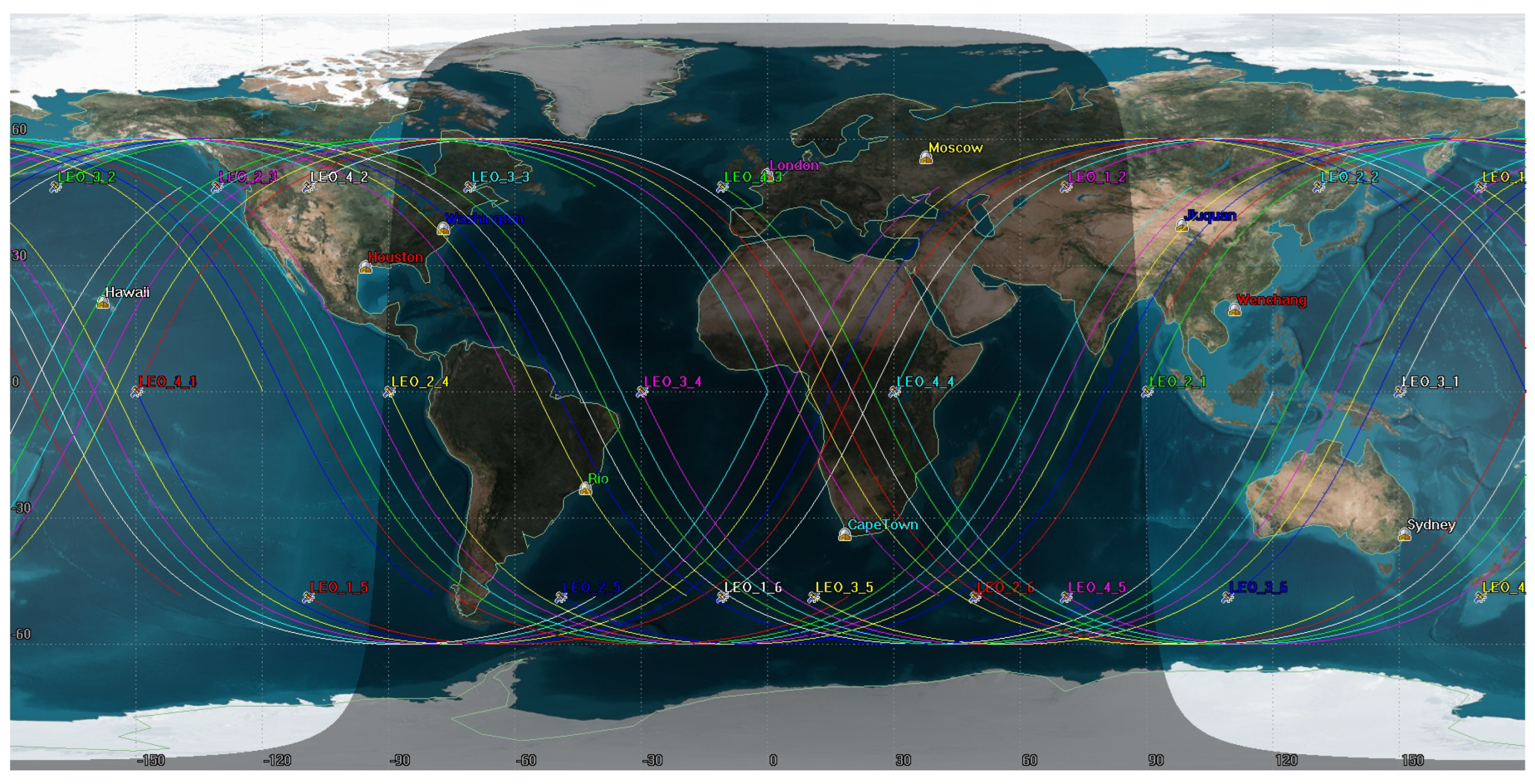
To verify the effectiveness of the RR-MPF algorithm, we implemented a satellite simulation using STK10 for orbital modeling and MATLAB-R2026a for traffic generation. The simulation scenario is illustrated in Figure 4. The scenario comprised two source ground stations transmitting via 24 LEO relay satellites to two destination ground stations. Traffic followed a Pareto distribution over 36 time slots spanning 3 h. The satellite network and simulation parameters are shown in Table 1 and Table 2. The STK scenario file of the simulation scene and the main program code are available in the Supplementary Materials.

Figure 4. Simulation scene. The icons denote the 24 LEO relay satellites, and several ground stations. The shaded area indicates the night side of the Earth at the initial epoch.

Table 1. The satellite network parameters.

Satellite Parameter	Parameter Value
Number of orbital planes	4
Satellites per plane	6
Satellite altitude	1640 km
Orbital inclination	${60.0}^{\circ }$
RAAN	${30.0}^{\circ }$
Channel power gain	10 dB

Table 2. The simulation parameters.

Simulation Parameter	Parameter Value
Queue type	FIFO
Bandwidth	200 Mbps
Simulation time	180 min
Packet size	64–3000 B
Packet sending rate	400–600 pps
Satellite processing rate	0.8 GHz
Cache queue capacity	1024 MB

All comparative results for the four algorithms are averaged over 30 independent simulation runs with different random seeds. Traffic is generated by Pareto-distributed ON/OFF sources, and each figure point is the average of these runs, ensuring statistically consistent comparisons.

The simulation also models handover-induced in-flight packet loss: in the last slot before an ISL or feeder switchover, packets on that link incur an additional loss factor of $0.008$ and a 5 ms handover delay. This cost is invisible to per-link scoring and can only be anticipated via the Markov forecast in Section 3. Each benchmark re-optimizes at its own re-planning period (Table 3) and retains its current path between re-planning instants unless it breaks.

Table 3. Algorithm and statistical-protocol parameters.

Parameter	Value
Pheromone importance factor $\alpha$	1.0
Heuristic importance factor $\beta$	2.0
Evaporation coefficient $\rho$	0.1
Pheromone deposit constant Q	1.0
Number of ants $N_{\mathrm{ants}}$	40
Number of iterations $N_{\mathrm{iter}}$	60
Sliding-window size W (transition estimation)	10 slots
Time slot duration $\Delta t$	300 s
Cross-slot weights ${\zeta }_1,{\zeta }_2$	0.65, 0.35
Metric weight vector $\vartheta$	[0.25, 0.25, 0.25, 0.25]
DPSO-TA swarm size/iterations	30/50
GA-CG population/iterations/mutation rate	30/50/0.1
Benchmark re-planning period (iVACO/GA-CG/DPSO-TA)	2/3/6 slots
Independent runs per configuration	30

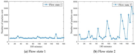
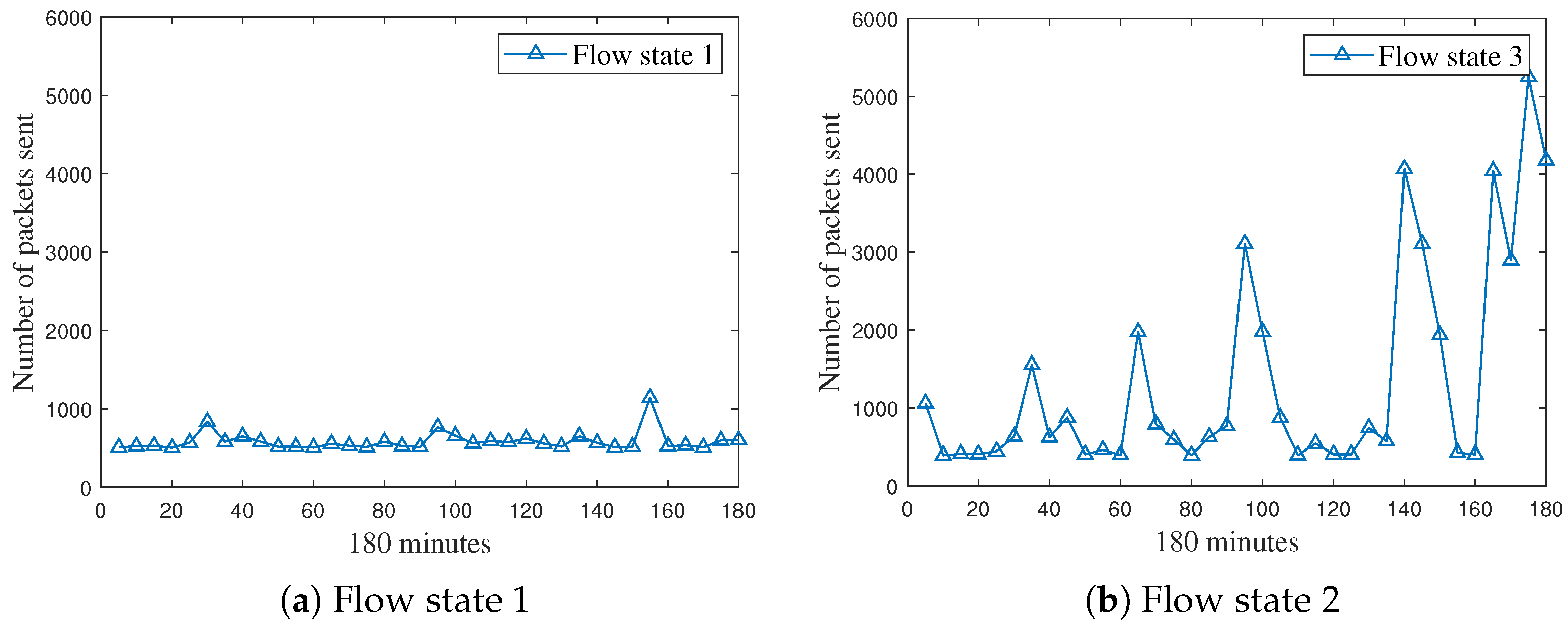
The data flow follows a Pareto distribution. Two scenarios are derived from measured traffic curves (Figure 5): a low-volatility state (state 1, std/mean $=21\%$, mean load $\approx 582$ packets per slot) and a high-volatility state (state 2, std/mean $=101\%$, mean load $\approx 1336$ packets per slot), with per-slot profiles from 36 five-minute samples over a 180 min window. In state 1, the load stays within a narrow band around its mean; in state 2, the mean load doubles and burst peaks exceed 5000 packets per slot, driving shared edges close to service capacity. Packets are sent from the source ground station and destination ground station over the satellite network for 180 min. The reported end-to-end path reliability is the effective reliability: the reliability degree of Definition 5 averaged along the selected path, scaled by the fraction of packets delivered over that path.

Figure 5. Number of packets sent in different flow states.

Configuration of Markov Transition Probabilities

In the simulations, the parameters $\lambda$ and $\mu$ act as telemetry-triggered rules that shape the state transition behavior in the simulation log (e.g., imminent visibility loss increases the failure intensity). The transition matrix ${\mathbf{P}}^r$ is not set directly from $\lambda$ and $\mu$; it is estimated from the observed transition counts via the maximum-likelihood estimator of Equation (15).

To ensure the reproducibility of the proposed reliability model, we detail the derivation of the Markov chain parameters $\lambda$ (failure transition rate) and $\mu$ (repair transition rate) within the simulation environment. These parameters are dynamically inferred from real-time network telemetry generated by the co-simulation platform.

• Failure Transition Rate ($\lambda$): The probability of a link transitioning to a lower reliability state (e.g., from $s_1$ to $s_2$) is governed by two observable risk factors extracted from the simulation log:
  • Geometric Visibility: As detailed in Table 1, the satellite constellation is modeled in STK. At each time slot $\Delta t$, the STK access report is queried; if the residual line-of-sight duration for link $e_k^{v^i,v^j}$ falls below the slot duration (i.e., the link is predicted to disconnect within $\Delta t$), $\lambda$ is set to a high value of $0.8$.
  • Queue Congestion: Referring to the node service capacity specified in Table 2, the peak server utilization u at node $v^i$ over the slot’s sub-intervals is monitored. If the peak utilization exceeds $75\%$ of the node service capacity, indicating imminent congestion and packet loss, $\lambda$ is set to $0.6$, unless already elevated by the visibility condition.
  In the absence of these triggering conditions, a baseline failure rate of $\lambda =0.05$ is maintained to account for random channel fluctuations.
• Repair Transition Rate ($\mu$): The recovery probability is set to a constant $0.3$ once the triggering failure condition (visibility loss or congestion) is resolved. This value reflects the average rate at which alternative paths are established or backlogged queues are drained in the simulated STIN environment.

5.2. Network Reliability Modeling

In this section, network and traffic statistics are collected, and the RR-MPF routing algorithm is applied to compute the optimal path performance parameters under varying traffic growth coefficients. Furthermore, the link switching delay induced by node movement is simulated by introducing a disturbance delay. Both transmission delay and queueing delay are considered to compute the average traffic delay. The packet drop rate resulting from queue overflow during transmission is calculated, and delay variance is quantified by statistically analyzing the time-series data to characterize transmission jitter.

A Markov process model is employed to characterize network performance indices within each discrete time slot. Link reliability under varying traffic conditions is computed using the multi-metric model of Section 3 (Equation (12)), yielding a reliability range of $[0.00,1.00]$ that is quantized into the same three levels defined in Section 3.2. These three reliability levels are defined as follows:

• Normal operation state (I): reliability interval $[0.80,1.00]$.
• Minor degradation state (II): reliability interval $[0.40,0.80)$.
• Failure state (III): reliability interval $[0.00,0.40)$.

5.3. Routing Result Analysis

RR-MPF integrates multi-slot state analysis for optimal path computation. To demonstrate the advantage of RR-MPF over other algorithms in terms of network reliability, we compare RR-MPF with iVACO [31], DPSO-TA [32], and GA-CG [33]. These three methods are selected as representative metaheuristic routing algorithms that belong to the same ACO/PSO/GA families as our solver. Although they were not originally designed for STINs, they share the same underlying optimization paradigm, so the comparison isolates the benefit of the proposed reliability forecast model rather than that of the optimization engine.

iVACO is an improved self-organizing network routing algorithm that models the network as a graph and uses an ant pheromone-based communication mechanism to find optimal or near-optimal routes between nodes. It can handle multiple QoS requirements simultaneously and provide trade-offs among different QoS metrics. DPSO-TA accounts for the periodicity of time-triggered flows, defines a utility function, and optimizes the task assignment problem through iterative improvement. It also applies a load balancing mechanism across multiple hosts, thereby reducing task completion time and minimizing the failure rate. GA-CG employs a genetic algorithm to optimize the reverse propagation process, significantly reducing computation time while obtaining high-quality solutions to the multi-path node scheduling problem.

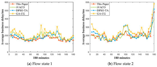
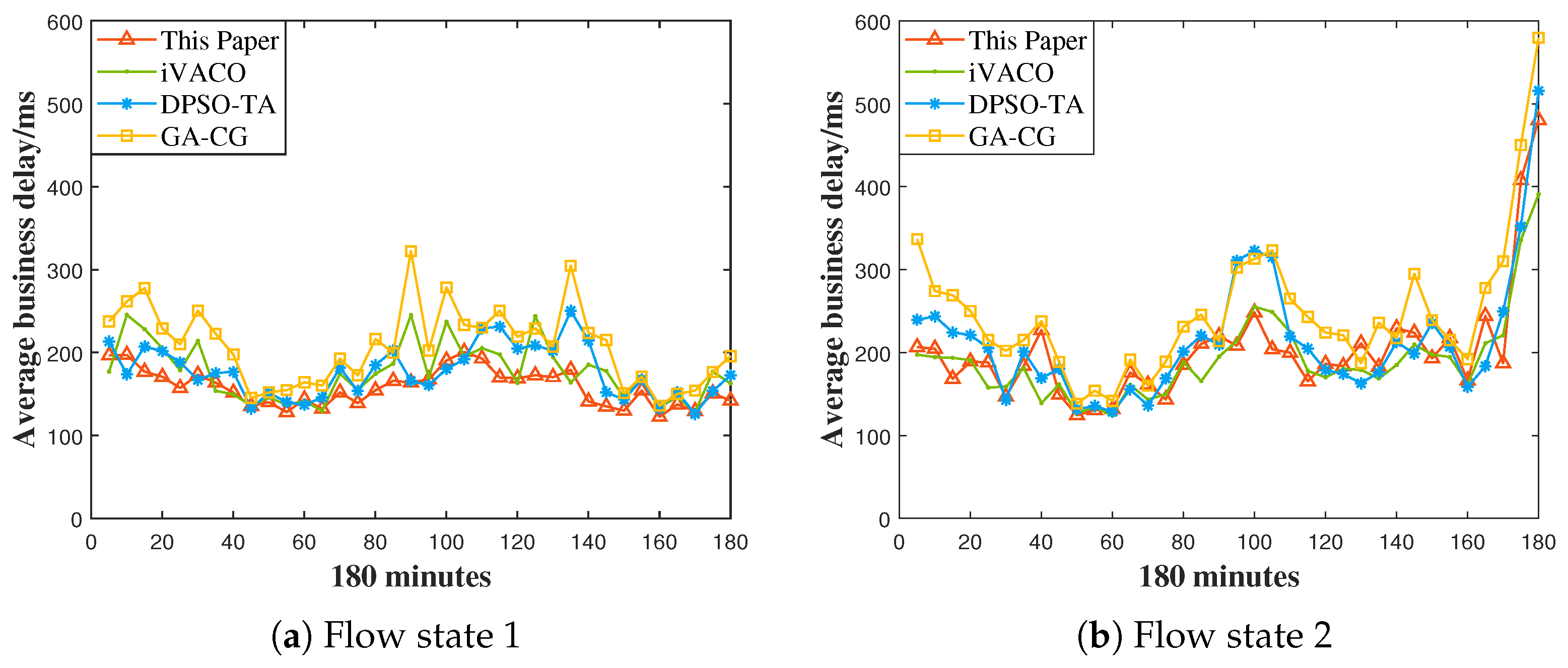
We compute the average end-to-end link delay of network traffic from source to destination using the four algorithms under different traffic states. The numerical results are shown in Figure 6.

Figure 6. Network average traffic delay by using different routing algorithm in different traffic scenarios.

As shown in Figure 6, under low traffic the link delay trend of RR-MPF aligns with those of the benchmark algorithms, where delay is governed primarily by the propagation component. In state 2, sustained bursts congest shared edges, and the per-link backlog accumulates and drains only gradually, so the mean delay rises from 158.3 ms in state 1 to 202.4 ms and stays elevated after each burst subsides (the cumulative-delay regime in Figure 6b). Because the forecast steers RR-MPF away from backlog-accumulating edges, the benchmark curves diverge increasingly from RR-MPF as volatility grows. Unlike the benchmarks, RR-MPF selects links by comprehensive reliability during traffic bursts while accounting for the projected link state at time $k+1$. This cross-slot consideration improves path selection in dynamic space environments. In the low-volatility state, RR-MPF reduces the average routing path delay by 10.6%, 10.6%, and 23.9% compared with iVACO, DPSO-TA, and GA-CG, respectively; in the high-volatility state, it remains 5.3% and 18.6% below DPSO-TA and GA-CG, and is statistically comparable to iVACO, whose frequent replanning keeps its mean delay low at the cost of reliability and drop rate.

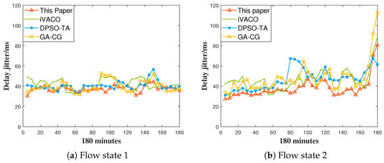
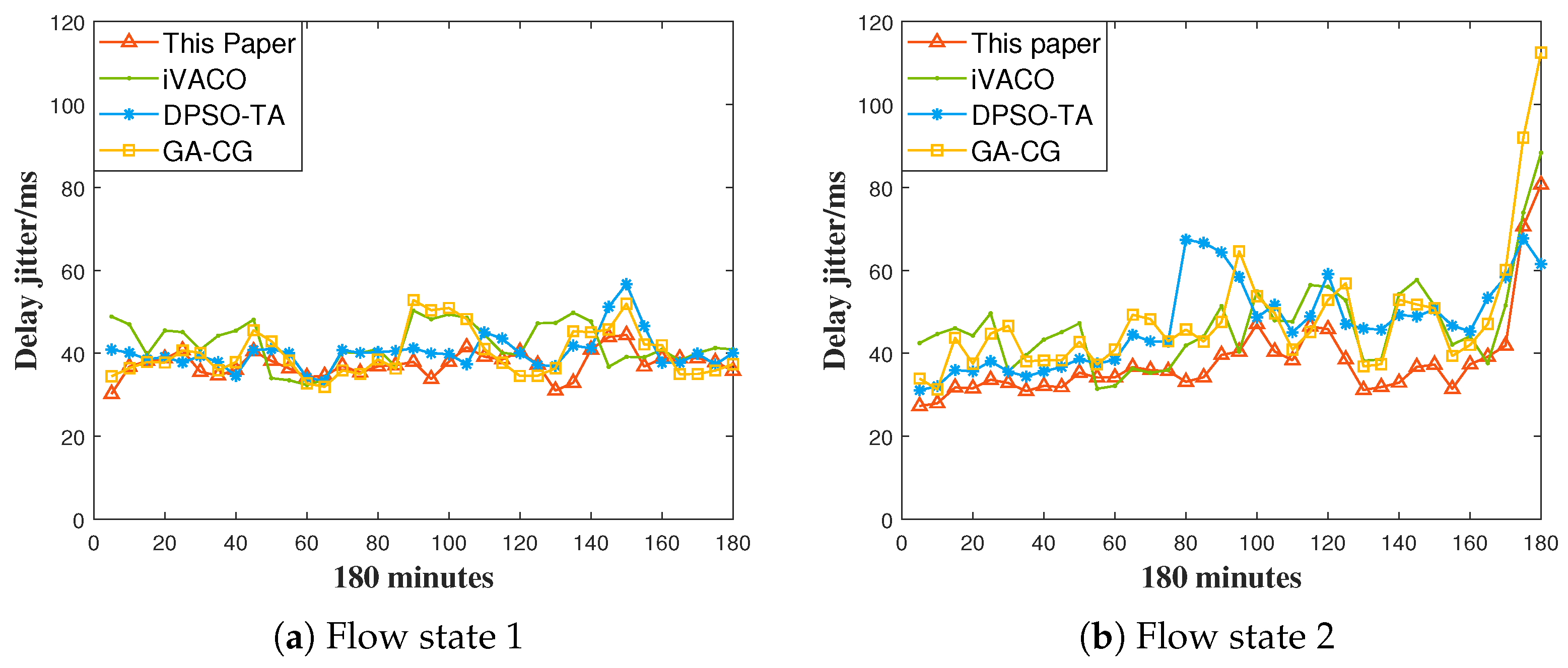
We calculate the delay jitter of network traffic from source to destination nodes using the four algorithms across different traffic state scenarios. The numerical results in Figure 7 reveal trends similar to those observed for service delay variation. When network traffic bursts, the cache queue becomes fully occupied and the satellite node cannot process the backlog of packets in time, resulting in a sharp increase in traffic latency. Furthermore, owing to differences in data burst patterns, delay variation intensifies and jitter increases. In scenarios with small traffic fluctuations, the overall low traffic load maintains a favorable delay state with minimal jitter. The RR-MPF algorithm accounts for the relationship between arrival rate and service rate and computes queueing delay over a long-term horizon. As the traffic fluctuation coefficient increases, delay jitter rises noticeably: the mean jitter of RR-MPF grows from 37.4 ms (state 1) to 38.0 ms (state 2), while the benchmark algorithms climb to 40.0–42.4 ms and 46.7–48.2 ms, respectively. Compared with iVACO, DPSO-TA, and GA-CG, RR-MPF reduces the link delay jitter by 11.7%, 7.1%, and 6.4% in the low-volatility state and by 18.7%, 19.1%, and 21.3% in the high-volatility state, respectively.

Figure 7. Network delay jitter by using different routing algorithms in different traffic scenarios.

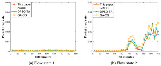
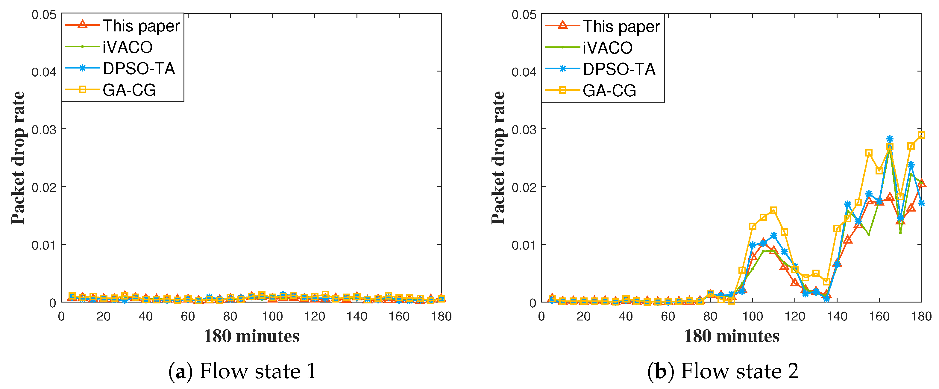
We calculate the packet drop rate of network traffic from source to destination nodes using the four algorithms in different traffic state scenarios. Numerical results are shown in Figure 8. Under small traffic fluctuations, the packet drop rates of all four algorithms remain relatively stable, increasing only slightly during occasional traffic bursts. Under severe traffic instability, the paths selected by each algorithm experience a significant increase in packet drop rate due to buffer overflow. The RR-MPF algorithm accounts for link performance at both the current time k and the next time $k+1$, effectively handling scenarios with large traffic bursts. The mean packet drop rate grows from 0.055% (state 1) to 0.51% (state 2), and RR-MPF keeps the lowest drop rate in every state. In the high-burst state, RR-MPF holds the drop rate at 0.51% against 0.55–0.78% for the benchmarks, and the gap widens during each congestion episode. Compared with iVACO, DPSO-TA, and GA-CG, RR-MPF reduces the end-to-end packet drop rate by 10.4%, 10.6%, and 25.8% in the low-volatility state and by 6.8%, 15.2%, and 34.4% in the high-volatility state, respectively.

Figure 8. Network packet drop rate by using different routing algorithms in different traffic scenarios.

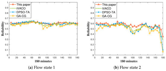
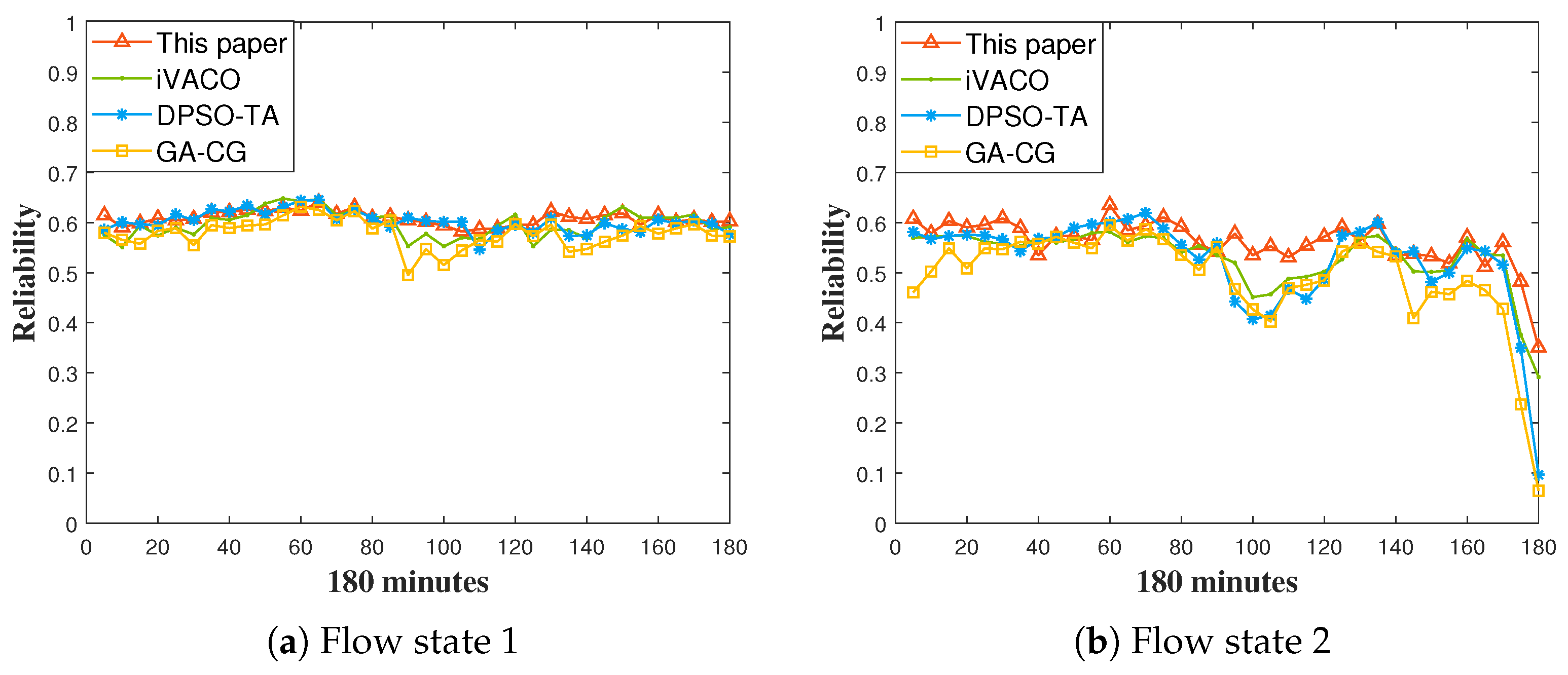
Figure 9 compares the reliability of the three benchmark algorithms against RR-MPF across various traffic state scenarios. RR-MPF accounts for multi-factor link performance at the current time and computes the reliability transition probability via a Markov process, selecting the path with the best weighted reliability for both the current and the next time slot. In high traffic burst scenarios, RR-MPF selects transmission paths with higher reliability, thereby effectively avoiding disturbances caused by link switching and queueing delays. The mean effective path reliability decreases from 0.609 (state 1) to 0.561 (state 2) for RR-MPF. RR-MPF attains the highest mean effective path reliability in both traffic states, with the largest advantage in the high-burst state: 5.8%, 6.9%, and 14.0% over iVACO, DPSO-TA, and GA-CG ($0.561$ vs. $0.530$, $0.525$, and $0.493$, respectively), against state 1 gains of 1.9%, 1.2%, and 5.3%; paired t-tests over the 30 runs confirm that these differences are significant in state 2. Compared with iVACO, DPSO-TA, and GA-CG, RR-MPF improves the overall path reliability by up to 14.0%, with gains of 3.7–9.2% averaged over the two states.

Figure 9. Network reliability by using different routing algorithms in different traffic scenarios.

Table 4 shows that the proposed algorithm matches or outperforms the other three algorithms in both traffic states, with its advantage growing as the traffic burst intensifies. When the traffic burst is large, the proposed algorithm considers both the end-to-end link reliability state in the current time slot and the state transition probability in the next time slot. Consequently, its average end-to-end link reliability is higher than that of the other three algorithms when facing large-scale traffic bursts.

Table 4. The average reliability of the routing path.

Algorithm	Flow 1	Flow 2
RR-MPF	0.609	0.561
iVACO	0.598	0.530
DPSO-TA	0.602	0.525
GA-CG	0.578	0.493

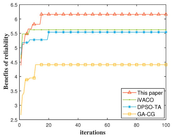
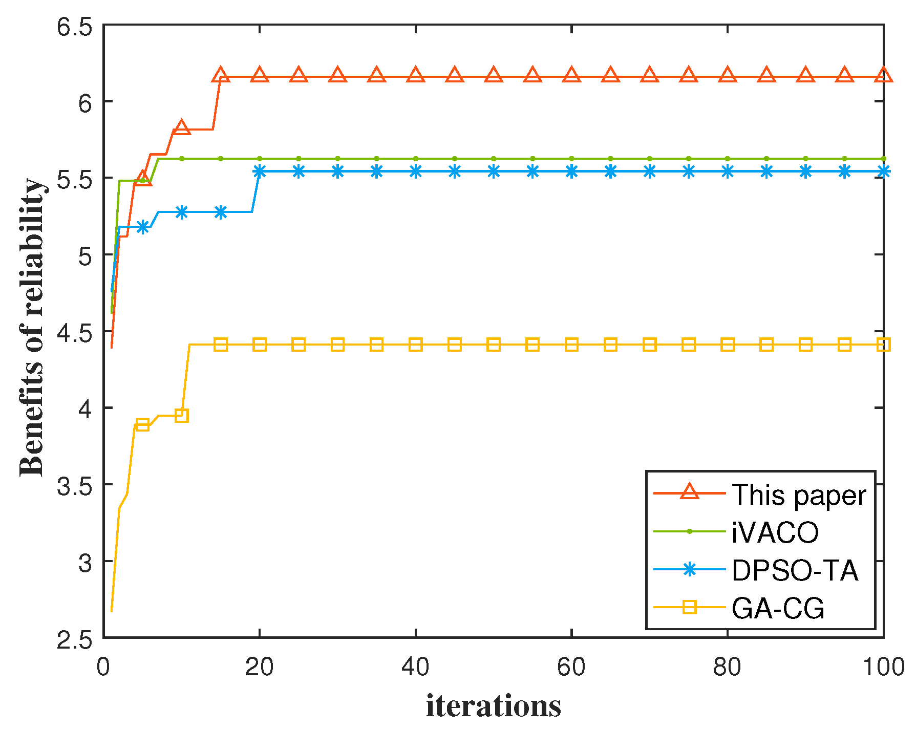
We examine the impact of different link states on routing path reliability. As shown in Figure 10, RR-MPF is particularly effective in mitigating the negative effects of link switching across multiple time slots, thereby ensuring the highest reliability and service continuity for satellite services. In terms of the final convergence value, RR-MPF achieves the largest improvement in routing path quality, followed by iVACO and DPSO-TA. GA-CG lacks directional optimization during cross-mutation iterations and depends heavily on the initial population, which limits its convergence performance.

Figure 10. Reliability benefit convergence curve of four algorithms.

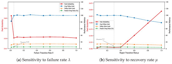
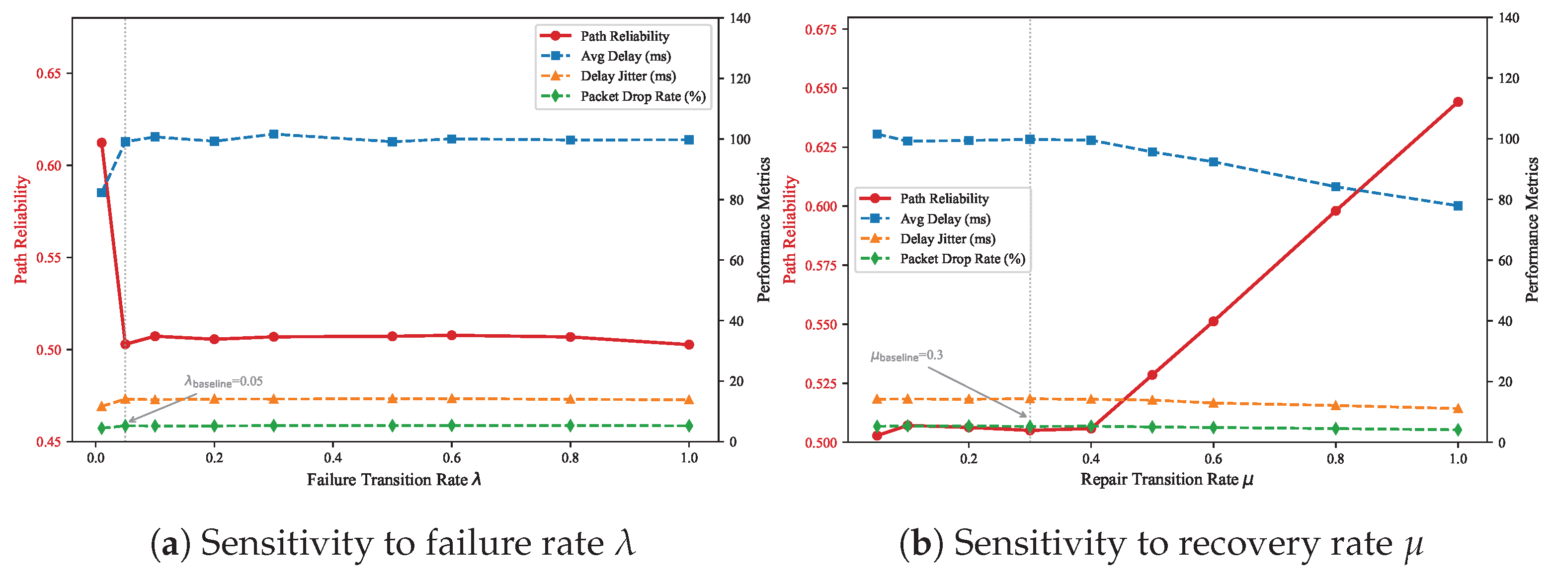
To evaluate the robustness of RR-MPF with respect to the Markov model parameters, we conducted a sensitivity analysis by varying the link failure rate $\lambda \in [0.01,1.0]$ and the recovery rate $\mu \in [0.05,1.0]$ while keeping other parameters fixed. As shown in Figure 11a, the routing reliability of RR-MPF falls from $0.612$ at very small $\lambda$ to about $0.503$ at the operating point $\lambda =0.05$, and then remains essentially flat ($0.503$–$0.507$) up to $\lambda =1.0$: beyond the operating point, additional random failures no longer change the achieved path quality, and the delay, jitter, and drop rate curves stay nearly flat over the entire sweep. As shown in Figure 11b, the reliability stays within $0.503$–$0.508$ for $\mu \le 0.4$ and then rises steeply to $0.645$ at $\mu =1.0$: faster recovery improves the routing outcome only once the recovery rate becomes comparable to the disturbance rate, while the average delay decreases mildly with $\mu$. The chosen operating point ($\lambda =0.05$, $\mu =0.3$) thus lies in the flat region of both sweeps, so small parameter deviations do not qualitatively alter the routing outcome.

Figure 11. Sensitivity analysis of Markov parameters: (a) link failure rate $\lambda$; (b) link recovery rate $\mu$. The shaded region indicates the parameter range used in the main experiments ($\lambda =0.05$, $\mu =0.3$).

5.4. Additional Analyses

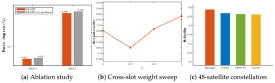
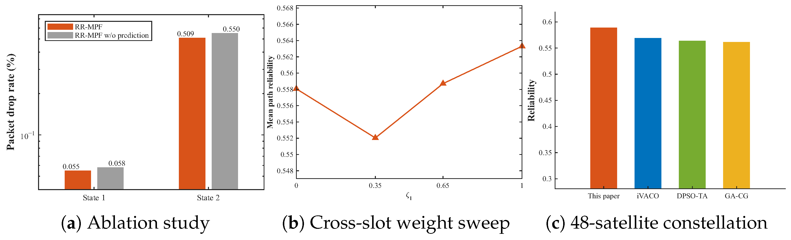
This subsection reports additional analyses that complement the main evaluation: two evaluation indicators that do not enter the optimization objective, an ablation study isolating the contribution of the Markov forecast, a sensitivity analysis, and a scalability experiment on a larger constellation. Figure 12 summarizes the ablation study, the cross-slot weight sweep, and the scalability experiment.

Figure 12. Additional analyses: (a) packet drop rate of RR-MPF with and without the Markov forecast (ablation study); (b) mean path reliability versus the cross-slot weight ${\zeta }_1$; (c) mean path reliability in the 48-satellite constellation.

5.4.1. Independent Evaluation Indicators

The multi-metric reliability degree in Figure 9 and Table 4 shares its model with the optimization objective; the delivered-packet factor is computed post-decision and is external to it. To avoid circular evaluation, we report two further indicators that do not enter the objective at all: the number of path switches (re-routing events) per session and the service completion ratio (delivered/transmitted packets). Averaged over 30 independent runs, RR-MPF attains a switching count (40.9/41.9 per session in states 1–2) comparable to the benchmarks (35.3–40.2), and the service completion ratios of all four algorithms are clustered between 0.992 and 0.999, with RR-MPF the highest in state 1 (0.999) and on par in state 2. Its reliability advantage is therefore not obtained at the cost of excessive re-routing or degraded service completion.

5.4.2. Ablation Study

To isolate the benefit of forecasting, we evaluate a variant “RR-MPF w/o prediction” in which the forecast term is disabled (${\zeta }_2=0$) while the multi-metric reliability model, the ACO framework, and the seed schedule are kept identical (paired runs with common random numbers). As shown in Figure 12a, disabling the forecast component leaves the packet drop rate almost unchanged in the low-dynamic state (0.055% vs. 0.058%) but raises it noticeably in the high-dynamic state (0.509% vs. 0.550%), where the w/o variant falls back to the level of the strongest benchmark; the same trend appears in the mean end-to-end delay (158.3 vs. 160.0 ms and 202.4 vs. 209.8 ms; the state 2 differences are significant in the paired t-tests), while the mean effective path reliability remains essentially unchanged (0.609 vs. 0.610, $p=0.41$; 0.561 vs. 0.563, $p=0.045$). The benefit of forecasting is therefore mainly operational and grows with the dynamics: it converts predictable disruptions (imminent switchover or congestion build-up) into proactive re-routing, cutting packet loss by 5–8% and delay by up to 3.5%, rather than raising the mean reliability value itself.

5.4.3. Sensitivity Analysis

Three additional studies examine the sensitivity to the remaining model parameters: (i) the cross-slot weights ${\zeta }_1/{\zeta }_2$ swept over $\{0,0.35,0.65,1\}$ (Figure 12b), where the mean path reliability in the high-volatility state stays within 0.552–0.563 over the entire sweep (about 1 percentage point), with the operating point ${\zeta }_1=0.65$ (0.559) lying mid-band; the flat profile indicates that the gain comes from the forecast-triggered re-routing rather than from a finely tuned weighting; (ii) the metric weight vector $\vartheta$ changed from the equal-weight setting to toughness-heavy and drop-heavy variants, yielding 0.559–0.618 and confirming that no weighting choice alters the conclusions; and (iii) the reliability state thresholds varied over (0.80/0.40), (0.75/0.35), and (0.85/0.45), yielding 0.548–0.573 and showing that the routing behavior is consistent.

5.4.4. Scalability to a 48-Satellite Constellation

To examine scalability, we evaluate a 48-satellite (8 planes × 6 satellites) constellation under traffic state 2 (the most demanding scenario), with two simultaneously routed flows. As shown in Figure 12c, in this setting, RR-MPF sustains a mean effective path reliability of 0.589 against 0.569 for the strongest benchmark (iVACO, a 3.5% relative improvement) and reduces the average end-to-end delay from 206.4 ms to 165.6 ms; its background prediction thread completes in 19.4 ms and the online routing decision in about 0.37 s per slot, both well below the 300 s slot duration. The framework thus scales to constellations of this size without violating its real-time constraints; extension to mega-constellations is identified as future work.

6. Conclusions

This paper presented a reliability analysis of Satellite–Terrestrial Integrated Networks based on a multi-state Markov reliability model, in which link quality is categorized into discrete levels to capture time-varying dynamics. Building on this model, we proposed RR-MPF, an enhanced Ant Colony Optimization algorithm that selects routing paths by maximizing a cross-slot weighted objective over both the current link reliability and the forecast state distribution in the subsequent time slot. Extensive simulations under two measured traffic scenarios (low- and high-volatility states) show that RR-MPF reduces the average end-to-end delay by up to 23.9%, the delay jitter by 6.4%–21.3%, and the packet drop rate by 6.8%–34.4% relative to iVACO, DPSO-TA, and GA-CG, while improving the overall path reliability by up to 14.0%, with the reliability gain concentrated in the high-volatility state (statistically significant, $p<0.05$). A 48-satellite extension confirms that the framework scales to medium-scale LEO constellations without violating its real-time constraints. These results indicate that incorporating parallel Markov forecasting into the routing plane enhances the resilience of STINs against topology-induced disruptions. Future work will extend the prediction horizon to multiple time slots and investigate scalability in mega-constellation deployments.

References

- Xu, S.; Liu, J.; Cao, Y.; Li, J.; Zhang, Y. Intelligent reflecting surface enabled secure cooperative transmission for satellite-terrestrial integrated networks. IEEE Trans. Veh. Technol. 2021, 70, 2007–2011. [Google Scholar] [CrossRef] [Scilit]
- Lin, Z.; Lin, M.; Wang, J.-B.; De Cola, T.; Wang, J. Joint beamforming and power allocation for satellite-terrestrial integrated networks with non-orthogonal multiple access. IEEE J. Sel. Top. Signal Process. 2019, 13, 657–670. [Google Scholar] [CrossRef] [Scilit]
- Zhang, N.; Zhang, S.; Yang, P.; Alhussein, O.; Zhuang, W.; Shen, X.S. Software defined space-air-ground integrated vehicular networks: Challenges and solutions. IEEE Commun. Mag. 2017, 55, 101–109. [Google Scholar] [CrossRef] [Scilit]
- Kodheli, O.; Lagunas, E.; Maturo, N.; Sharma, S.K.; Shankar, B.; Montoya, J.F.M.; Duncan, J.C.M.; Spano, D.; Chatzinotas, S.; Kisseleff, S.; et al. Satellite communications in the new space era: A survey and future challenges. IEEE Commun. Surv. Tutor. 2020, 23, 70–109. [Google Scholar] [CrossRef] [Scilit]
- Ball, M.O. Computational complexity of network reliability analysis: An overview. IEEE Trans. Reliab. 1986, 35, 230–239. [Google Scholar] [CrossRef] [Scilit]
- Lin, M.; Huang, Q.; De Cola, T.; Wang, J.-B.; Wang, J.; Guizani, M.; Wang, J.-Y. Integrated 5G-satellite networks: A perspective on physical layer reliability and security. IEEE Wirel. Commun. 2020, 27, 152–159. [Google Scholar] [CrossRef] [Scilit]
- Zhang, X.; Mahadevan, S. A game theoretic approach to network reliability assessment. IEEE Trans. Reliab. 2017, 66, 875–892. [Google Scholar] [CrossRef] [Scilit]
- Huang, D.-H.; Huang, C.-F.; Lin, Y.-K. A binding algorithm of lower boundary points generation for network reliability evaluation. IEEE Trans. Reliab. 2019, 69, 1087–1096. [Google Scholar] [CrossRef] [Scilit]
- Vasar, C.; Prostean, O.; Filip, I.; Robu, R.; Popescu, D. Markov models for wireless sensor network reliability. In Proceedings of the 2009 IEEE 5th International Conference on Intelligent Computer Communication and Processing; IEEE: New York, NY, USA, 2009; pp. 323–328. [Google Scholar]
- Kabir, S.; Papadopoulos, Y. Applications of Bayesian networks and Petri nets in safety, reliability, and risk assessments: A review. Saf. Sci. 2019, 115, 154–175. [Google Scholar] [CrossRef] [Scilit]
- Guo, X.; Ji, J.; Khan, F.; Ding, L.; Tong, Q. A novel fuzzy dynamic Bayesian network for dynamic risk assessment and uncertainty propagation quantification in uncertainty environment. Saf. Sci. 2021, 141, 105285. [Google Scholar] [CrossRef] [Scilit]
- Levitin, G.; Xing, L.; Amari, S.V. Recursive algorithm for reliability evaluation of non-repairable phased mission systems with binary elements. IEEE Trans. Reliab. 2012, 61, 533–542. [Google Scholar] [CrossRef] [Scilit]
- Altiparmak, F.; Dengiz, B.; Smith, A.E. A general neural network model for estimating telecommunications network reliability. IEEE Trans. Reliab. 2009, 58, 2–9. [Google Scholar] [CrossRef] [Scilit]
- Sharafat, A.R.; Ma’rouzi, O.R. All-terminal network reliability using recursive truncation algorithm. IEEE Trans. Reliab. 2009, 58, 338–347. [Google Scholar] [CrossRef] [Scilit]
- Fard, N.; Lee, T.-H. Spanning tree approach in all-terminal network reliability expansion. Comput. Commun. 2001, 24, 1348–1353. [Google Scholar] [CrossRef] [Scilit]
- Dugan, J.B.; Bavuso, S.J.; Boyd, M.A. Dynamic fault-tree models for fault-tolerant computer systems. IEEE Trans. Reliab. 1992, 41, 363–377. [Google Scholar] [CrossRef] [Scilit]
- Gao, X.; Ye, Z.; Fan, J.; Zhong, W.; Zhao, Y.; Cao, X.; Yu, H.; Qiao, C. Virtual network mapping for multicast services with max–min fairness of reliability. J. Opt. Commun. Netw. 2015, 7, 942–951. [Google Scholar] [CrossRef] [Scilit]
- Park, J.-H. All-terminal reliability analysis of wireless networks of redundant radio modules. IEEE Internet Things J. 2015, 3, 219–230. [Google Scholar] [CrossRef] [Scilit]
- Mo, Y.; Liang, M.; Xing, L.; Liao, J.; Liu, X. Network simplification and K-terminal reliability evaluation of sensor-cloud systems. IEEE Access 2020, 8, 177206–177218. [Google Scholar] [CrossRef] [Scilit]
- Jung, S.; Choi, J.P. End-to-end reliability of satellite communication network systems. IEEE Syst. J. 2020, 15, 791–801. [Google Scholar] [CrossRef] [Scilit]
- Yang, G.; Liang, T.; He, X.; Xiong, N. Global and local reliability-based routing protocol for wireless sensor networks. IEEE Internet Things J. 2018, 6, 3620–3632. [Google Scholar] [CrossRef] [Scilit]
- Inoue, T. Reliability analysis for disjoint paths. IEEE Trans. Reliab. 2018, 68, 985–998. [Google Scholar] [CrossRef] [Scilit]
- Liu, B.; Wei, X.; Hu, H.; Yu, P.; Shi, L. A reliable routing algorithm based on path satisfaction in the energy internet. Electronics 2025, 14, 393. [Google Scholar] [CrossRef] [Scilit]
- Chakraborty, S.; Goyal, N.K.; Mahapatra, S.; Soh, S. Minimal path-based reliability model for wireless sensor networks with multistate nodes. IEEE Trans. Reliab. 2019, 69, 382–400. [Google Scholar] [CrossRef]
- Xiang, S.; Yang, J. Reliability evaluation and reliability-based optimal design for wireless sensor networks. IEEE Syst. J. 2019, 14, 1752–1763. [Google Scholar] [CrossRef] [Scilit]
- Chen, Y.; Cao, H.; Wang, L.; Chen, D.; Liu, Z.; Zhou, Y.; Shi, J. Deep reinforcement learning-based routing method for low Earth orbit mega-constellation satellite networks with service function constraints. Sensors 2025, 25, 1232. [Google Scholar] [CrossRef] [Scilit]
- Al Homssi, B.; Al-Hourani, A.; Wang, K.; Conder, P.; Kandeepan, S.; Choi, J.; Allen, B.; Moores, B. Next generation mega satellite networks for access equality: Opportunities, challenges, and performance. IEEE Commun. Mag. 2022, 60, 18–24. [Google Scholar] [CrossRef] [Scilit]
- Nichols, K.; Jacobson, V. Controlling queue delay. Commun. ACM 2012, 55, 42–50. [Google Scholar] [CrossRef] [Scilit]
- Cruz, R.L. A calculus for network delay. I. Network elements in isolation. IEEE Trans. Inf. Theory 1991, 37, 114–131. [Google Scholar] [CrossRef] [Scilit]
- Hastings, W.K. Monte Carlo sampling methods using Markov chains and their applications. Biometrika 1970, 57, 97–109. [Google Scholar] [CrossRef]
- Goudarzi, F.; Asgari, H.; Al-Raweshidy, H.S. Traffic-aware VANET routing for city environments—A protocol based on ant colony optimization. IEEE Syst. J. 2018, 13, 571–581. [Google Scholar] [CrossRef] [Scilit]
- Baniabdelghany, H.; Obermaisser, R.; Khalifeh, A. Reliable task allocation for time-triggered IoT-WSN using discrete particle swarm optimization. IEEE Internet Things J. 2022, 9, 11974–11992. [Google Scholar] [CrossRef] [Scilit]
- Wang, C.; Guo, C.; Zuo, X. Solving multi-depot electric vehicle scheduling problem by column generation and genetic algorithm. Appl. Soft Comput. 2021, 112, 107774. [Google Scholar] [CrossRef] [Scilit]
- Krishnan, K.R. The convexity of loss rate in an Erlang loss system and sojourn in an Erlang delay system with respect to arrival and service rates. IEEE Trans. Commun. 1990, 38, 1314–1316. [Google Scholar] [CrossRef] [Scilit]
Disclaimer/Publisher’s Note: The statements, opinions and data contained in all publications are solely those of the individual author(s) and contributor(s) and not of MDPI and/or the editor(s). MDPI and/or the editor(s) disclaim responsibility for any injury to people or property resulting from any ideas, methods, instructions or products referred to in the content. |
© 2026 by the authors. Licensee MDPI, Basel, Switzerland. This article is an open access article distributed under the terms and conditions of the Creative Commons Attribution (CC BY) license.