Estimation of Forest Aboveground Biomass and Leaf Area Index Based on Digital Aerial Photograph Data in Northeast China

Abstract

Forest aboveground biomass (AGB) and leaf area index (LAI) are two important parameters for evaluating forest growth and health. It is of great significance to estimate AGB and LAI accurately using remote sensing technology. Considering the temporal resolution and data acquisition costs, digital aerial photographs (DAPs) from a digital camera mounted on an unmanned aerial vehicle or light, small aircraft have been widely used in forest inventory. In this study, the aerial photograph data was acquired on 5 and 9 June, 2017 by a Hasselblad60 digital camera of the CAF-LiCHy system in a Y-5 aircraft in the Mengjiagang forest farm of Northeast China, and the digital orthophoto mosaic (DOM) and photogrammetric point cloud (PPC) were generated from an aerial overlap photograph. Forest red-green-blue (RGB) vegetation indices and textural factors were extracted from the DOM. Forest vertical structure features and canopy cover were extracted from normalized PPC. Regression analysis was carried out considering only DOM data, only PPC data, and a combination of both. A recursive feature elimination (RFE) method using a random forest was used for variable selection. Four different machine-learning (ML) algorithms (random forest, k-nearest neighbor, Cubist and supporting vector machine) were used to build regression models. Experimental results showed that PPC data alone could estimate AGB, and DOM data alone could estimate LAI with relatively high accuracy. The combination of features from DOM and PPC data was the most effective, in all the experiments considered, for the estimation of AGB and LAI. The results showed that the height and coverage variables of PPC, texture mean value, and the visible differential vegetation index (VDVI) of the DOM are significantly related to the estimated AGB (R² = 0.73, RMSE = 20 t/ha). The results also showed that the canopy cover of PPC and green red ratio index (GRRI) of DOM are the most strongly related to the estimated LAI, and the height and coverage variables of PPC, the texture mean value and visible atmospherically resistant index (VARI), and the VDVI of DOM followed (R² = 0.79, RMSE = 0.48).

1. Introduction

Nowadays, global climate change is becoming a major challenge for current and future generations. Forests play crucial roles in adjusting the global and regional carbon cycle and bioenergy consumption. Forest aboveground biomass (AGB) is a key biophysical parameter. It can provide important vegetation information about growth, health, and productivity [1,2]. Also, it is often required by the implementation of effective climate policies [3,4]. Additionally, the leaf area index (LAI), another important biophysical parameter, could provide more detailed canopy structure information [5]. Therefore, the accurate estimation and prediction of these two forest parameters is of great importance.

Traditional forest investigation relies on manual ground measurements with intensive time and high costs, such as destructive individual tree sampling and non-destructive field measurements. The obvious advantage is that they can provide results with relatively high accuracy [6,7]. In an attempt to obtain a more efficient estimation of forest parameters under different scales and in various environments, remote sensing techniques have been commonly applied over the past few decades. Data obtained from different sensors, such as optical cameras [8,9,10], radar [11,12], and terrestrial [13,14,15] or airborne [16,17,18] light detection and ranging (LiDAR), are significantly more efficient and have a lower cost than laborious ground-based estimation methods and have become widely used to characterize forest structure [19].

It is known that AGB and LAI cannot be directly obtained using remote sensing techniques; they are usually estimated by establishing a regression relationship between parameters derived from remote sensing data. However, it is worth noting that one problem when using optical remote sensing or radar data for estimation is saturation. Therefore, under high biomass or canopy density, the estimation accuracy, especially for biomass, is often under estimation [12,20,21]. LiDAR can provide quite accurate 3-D information and a reliable estimation, but the cost to obtain data is high; therefore, it is not suitable for continuous monitoring over large areas.

In order to obtain accurate results, many researchers have tried to combine multispectral and textural information from optical remote sensing data and vertical structure information from LiDAR data to estimate forest parameters [22,23,24,25,26]. These findings have demonstrated that estimation accuracy could be improved by making most use of the potential by combining these two types of data [27,28].

However, due to the influence of cloud and haze, it is sometimes difficult for satellites to capture high-quality images in the short term. On the other hand, and as mentioned above, LiDAR data acquisition and processing costs are too high to perform monitoring of large forest areas [29]. Both satellite remote sensing and LiDAR data have some limitations in high phase and extensive forest inventory applications.

With the recent development of unmanned aerial vehicle (UAV) technology over the past few years, aerial photographs from a digital camera mounted on an UAV or light, small aircraft have been widely used in forest inventory [30,31,32,33,34,35], and they generally have good affordability and availability. One thing should be mentioned here is that most of the relevant research used either digital orthophoto mosaic (DOM) or photogrammetric point cloud (PPC). Dandois et al. [36] used “Structure from Motion (SfM)” computer vision algorithms to extract canopy structure and spectral attributes based on red-green-blue (RGB) aerial images. Understory digital terrain models (DTMs) and canopy height models (CHMs) were generated from leaf-on and leaf-off point clouds using procedures commonly applied to LiDAR point clouds. CHMs were strong predictors of field-measured tree heights (R² = 0.63–0.84). Mathews et al. [35] also used SfM computer vision algorithms to obtain high-density point clouds. Points near samples were extracted and input into a stepwise regression model to predict LAI. The final R² value was approximately 0.57. Ota et al. [37] investigated the capabilities of CHM derived from aerial photographs using the SfM approach to estimate AGB in a tropical forest and yielded an accurate estimate (R² = 0.79). These successful applications show the potential of the SfM algorithm.

In addition, recent advances in commercial software based on computer vision algorithms such as Pix4DMapper (https://pix4d.com/, Pix4D S.A. Lausanne, Switzerland) and Agisoft Photoscan (https://www.agisoft.com/, Agisoft LLC, St. Petersburg, Russia) have enabled the mass production of digital surface models (DSMs) using the SfM algorithm with a much higher level of automation and much greater ease of use [38]. Applying the SfM approach enables us to produce high spatial resolution photogrammetric point clouds with vertical structure features similar to those derived from airborne LiDAR and DOM similar to satellite optical images with horizontal features.

In terms of the regression model used for building the relationship, many researchers have applied machine-learning methods in forest inventory and have obtained better accuracy in the past few years [39,40]. It is well known that the near-infrared (NIR) domain is a good indicator of vegetation health; we imitated the structure of the NIR band to construct the vegetation indices based on only red-green-blue three spectral bands in this study. To fully explore the advantages of digital aerial photographs (only RGB bands, not including the NIR band) in forest inventory, we focus on the estimation of AGB and LAI based on only DOM, only PPC, and DOM + PPC using a machine-learning method. This study will achieve the following goals: (1) processing digital aerial photograph (DAP) data based on the SfM approach to generate PPC and DOM and (2) estimating forest AGB and LAI based on only DOM, only PPC, and a combination of both.

2. Materials and Methods

2.1. Study Area

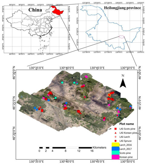
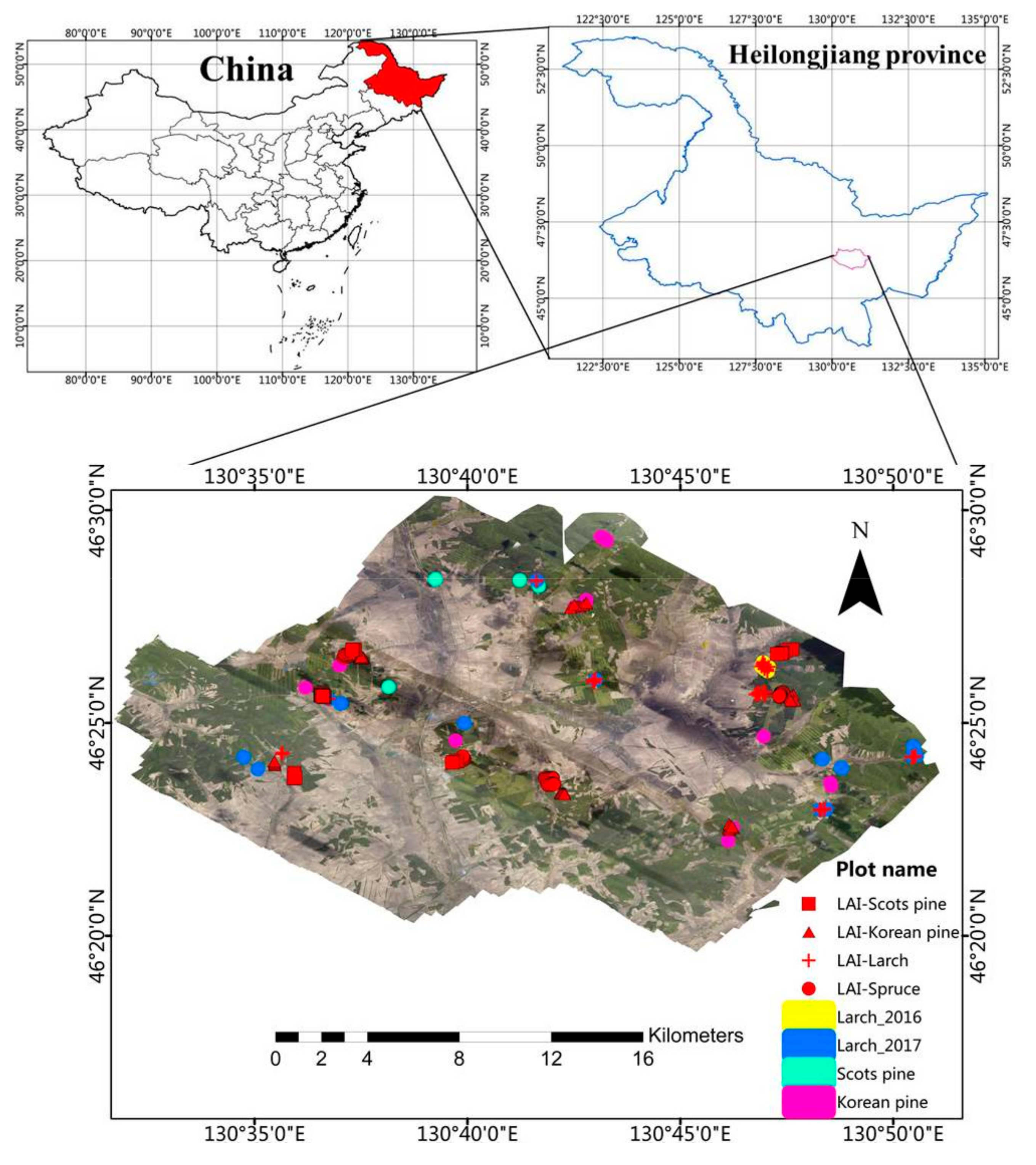
The study area is located at the Mengjiagang forest farm (46°26′ N, 130°43′ E) of Jiamusi city, in Heilongjiang Province of China (Figure 1), which is influenced by a temperate continental climate. Annual precipitation occurs mainly in summer. The study area covers an approximate land area of 260 km², which varies in elevation from about 180 m to 450 m above sea level. The land is relatively flat without an extreme slope. The dominant tree species is Larch (Larix gmelinii (Rupr.) Rupr.), followed by Korean pine (Pinus koraiensis Sieb. et Zucc.), Scots pine (Pinus sylvestris L.var. mongolica Litv.), and Spruce (Picea asperata Mast).

Figure 1. Location of the study area and distribution of field measurements. Red “■, ▲, +, ●” points are the sites of center coordinates of the Scots pine, Korean pine, Larch and Spruce, respectively, for LAI observations. Yellow locations are the sites of Larch plots in 2016. Dark blue locations are the sites of Larch plots in 2017. Light blue locations are the sites of Scots pine plots. Purple locations are the sites of Korean pine plots.

2.2. Data

The research data include (1) digital aerial photograph (DAP) data (year 2017), (2) 0.25 m spatial resolution DEM from LiDAR (year 2017), (3) LAI field data (year 2017), and (4) field measured data (year 2017 and 2016).

2.2.1. DAP Data Collection

DAP and LiDAR data were acquired at the same time on 5 and 9 June 2017 by the Chinese Academy of Forestry (CAF) using a Hasselblad60 digital camera and Riegl LMS-Q680i of CAF-LiCHy system in a Y-5 aircraft. The average flight altitudes were 950 m and 1250 m above ground level (AGL), and the mean ground sampling distance (GSD) of DAP images was 9 cm and 13 cm, respectively. The average flight speed was 40 m/s, and the mean forward overlap (FO) and the mean overlap between flight lines of DAP images were about 70% and 50%, respectively. In terms of aerial photograph data, the camera focal length, image size, and pixel size inside the camera are 50 mm, 8964 × 6716 pixels, and 6.0 µm respectively. The details of the flight parameters are shown in Table 1.

Table 1. Details of digital aerial photograph and LiDAR data specifications.

Flight Conditions
Flight altitude (above-ground)	950 m, 1250 m
Flying speed	40 m/s
Acquisition time	5 and 9 June 2017
Digital Aerial Photograph: Hasselblad60
Focal length	50 mm
Spectral bands	red, green, blue
Forward overlap (FO)	70%
Overlap between flight lines	50%
Scale	8964 × 6716 pixels
Pixel size	6 µm
Ground resolution	9 cm, 13 cm
Average density of point cloud	11–26 pts/m2
LiDAR: Riegl LMS-Q680i
Wavelength	1550 nm
Laser pulse length	3 ns
Waveform sampling interval	1 ns
Laser beam divergence	0.5 mrad
Vertical resolution	15 cm, 20 cm
Pulse repetition rate	300 kHZ, 200 kHZ
Scan angle	±30°
Average density of point cloud	9.6 pts/m2, 6.3 pts/m2

2.2.2. Field Measurements

The standard plots were set based on comprehensive field exploration. The shape of the plot was rectangular, and the area of the plot was determined according to factors such as tree age, the density of the forest, and site quality. In this study, we chose three kinds of tree ages: mature forest, middle forest, and young forest. We established three density plot types: dense young tree plots, dense middle tree plots, and sparse mature large tree plots. There should be at least 50 trees in every plot in the mature forest, at least 70 trees in the middle forest, and at least 90 trees in the young forest.

According to this principle, an original area of 400 m² could be set in advance, and then the numbers of individual trees in each plot should be counted to determine the area of the plot. There were six different area sizes, which were 400 m² (20 m × 20 m), 600 m² (20 m × 30 m), 900 m² (30 m × 30 m), 1000 m² (25 m × 40 m), 1200 m² (30 m × 40 m), 1500 m² (30 m × 50 m). The numbers of plots of Korean pine, Scots pine, and Larch are 16, 5, and 35 respectively. The field data of 9 Larch plots were collected in July 2016. The field data of 26 Larch plots were collected under leaf-on canopy conditions from 4 to 20 June 2017. The field data of all Korean pine and Scots pine plots were measured from 20 to 30 August 2017. In addition to these three main tree species, there are Elm (Ulmus laciniata (Trautv.) Mayr), Linden (Tilia mandshurica Rupr. et Maxim), Aspen (Populus tomentosa Carr), Oak (Quercus mongolica Fisch. ex Ledeb.), Silver birch (Betula platyphylla Suk.), Maple birch (Betula costata Trautv.), Black birch (Betula davurica Pall.), and Ashtree (Fraxinus mandschurica Rupr.) in the plots. Fifteen Korean pine plots, three Scots pine plots, and nineteen Larch plots cover 600 m². One Scots pine plot covers 400 m². Nine Larch plots and one Scots pine plot cover 900 m². One Scots pine plot and one Larch plot cover 1000 m². Two Larch pine plots cover 1200 m². Four Larch pine plots cover 1500 m².

The quadrangle boundaries of field plots were firstly measured using GPS and tape. Based on the ground base station data, the accurate locations of plots were obtained by a differential global positioning system (DGPS). The differential total accuracy was between 0.5 m and 0.8 m.

Tree species, diameter at breast height (DBH), tree height, and the crown width of all living trees with a DBH greater than 5 cm were measured in each plot using tape or meters. The lengths of the east–west and south–north directions of the tree crown were measured with the tape, and the average value of two lengths was taken as the crown width. Tree species and DBH of all dead trees were measured. The statistical results of living trees are shown in Table 2.

Table 2. Summary of the field data (living trees).

Species	Number	Tree Height (m)		DBH (cm)
		Range	Mean	Range	Mean
Korean pine (Pinus koraiensis)	776	7.2–22.9	14.2	6.6–35.2	22.0
Scots pine (Pinus sylvestris)	215	12.9–30.6	20.3	15.3–43.6	25.0
Larch (Larix gmelinii)	3046	4.2–33.1	19.0	4.1–41.6	17.3
Elm (Ulmus laciniata)	9	8.7–15.4	11.2	7.1–11.0	8.8
Linden (Tilia mandshurica)	20	8.6–18.7	12.7	8.5–30.2	14.8
Aspen (Populus tomentosa)	6	14.3–17.3	15.9	15.0–27.0	17.9
Oak (Quercus mongolica)	63	7.2–19.8	11.2	6.4–24.4	9.2
Silver birch (Betula platyphylla)	154	9.6–21.5	14.2	6.2–26.6	11.0
Maple birch (Betula costata)	6	8.7–16.9	14.1	7.0–31.0	17.1
Black birch (Betula dahurica)	2	7.6–14.2	10.9	5.9–14.7	10.3
Ashtree (Fraxinus mandschurica)	10	7.5–15.5	13.8	10.0–16.3	12.1

We calculated the AGB of each measured living tree using these equations of different tree species based on tree height and DBH in Table 3.

Table 3. Aboveground biomass equations (AGB) of different tree species.

Tree Species	AGB Equation	Reference
Korean pine	WT = 0.027847(D2H)0.956544	[41]
Scots pine	WT = 0.3364D2.0067 + 0.2983D1.144 + 0.2931D0.8486
Larch	WT = 0.046238(D2H)0.905002
Birch	WT = 0.0278601(D2H)0.993386
Soft broad-leaf trees	WT = 0.0495502(D2H)0.952453
Silver birch	WT = 0.1193(D2H)0.8372 + 0.002(D2H)1.12 + 0.000015(D2H)1.47	[42]
Maple birch	WT = 0.07936(D2H)0.901 + 0.014167(D2H)0.764 + 0.01086(D2H)0.847
Black birch	WT = 0.14114(D2H)0.723 + 0.00724(D2H)1.0225 + 0.0079(D2H)0.8085
Elm	WT = 0.03146(D2H)1.032 + 0.007429D2.6745 + 0.002754D2.4965
Linden	WT = 0.01275(D2H)1.009 + 0.00824(D2H)0.975 + 0.00024(D2H)0.991
Oak	WT = 0.03141(D2H)0.733 + 0.002127D2.9504 + 0.00321D2.4735
Aspen	WT = 0.2286(D2H)0.6938 + 0.0247(D2H)0.7378 + 0.0108(D2H)0.8181
Ashtree	WT = 0.06013(D2H)0.891 + 0.00652(D2H)1.169 + 0.0044(D2H)0.9919

We only used the AGB of living trees in this study and did not consider the AGB of dead trees. The AGB of each plot was then calculated by summing up the AGB of each living tree.

We used two methods to calculate the AGB of living trees. One was on the basis of five tree species: Korean pine, Scots pine, Larch, Birch (Sliver birch, Maple birch and Black birch), and Soft broad-leaf trees (Aspen, Elm, Linden, Oak, and Ashtree). Another was on the basis of all 11 tree species. The statistical results of all plots are shown in Table 4. As we can see from Table 4, the results of the two methods are not very different. Thus, we used the AGB results of five tree species to build a model and analyze retrieval results in this study.

Table 4. Summary of field AGB (living trees).

Main Tree Species	Number of Plots	Number of Species 1	DOM		PPC		DOM + PPC		AGB (t/ha)
			T 2	V 3	T 2	V 3	T 2	V 3	Range	Mean	SD 4
Korean pine	16	5	11	5	11	5	13	3	83.64–180.90	107.89	21.86
		11							82.79–180.90	107.71	22.07
Scots pine	5	5	4	1	4	1	4	1	94.06–182.30	147.69	34.59
		11							94.06–182.30	147.69	34.59
Larch	35	5	24	11	24	11	23	12	81.25–261.84	142.84	39.34
		11							78.14–261.84	143.62	38.61

¹ The number of tree species used to calculate AGB. ² Training, the number of plots used to train in study result of the paper. ³ Validation, the number of plots used to validate in study result of the paper. ⁴ SD: standard deviation.

2.2.3. LAI Field Measurements

LAI field data were obtained from 5 to 20 June, 2017. There were 192 circular plots at a radius of 15 m. The LAI in each plot was measured using a LAI-2000 Plant Canopy Analyzer (https://www.licor.com/, LI-COR Corporate, Lincoln NE, USA). In total, 12 points in four perpendicular directions were measured in every plot, and the average value of 12 points was calculated as the field measured data. The central positions of these plots were first measured using a GPS instrument. Then, based on the ground base station data, the accurate locations of plots were obtained using DGPS. The differential total accuracy was between 0.5 m and 0.8 m. There are four species in the plots: Spruce (Picea asperata Mast), Korean pine (Pinus koraiensis Sieb. et Zucc.), Scots pine (Pinus sylvestris L. var. mongolica Litv.), and Larch (Larix gmelinii (Rupr.) Rupr.). The statistical results of the LAI field data are shown in Table 5.

Table 5. Summary of the leaf area index (LAI) field data.

Tree Species	Plot Amount	DOM		PPC		DOM + PPC		LAI Measured Value
		T 1	V 2	T 1	V 2	T 1	V 2	Range	Mean
Spruce	57	43	14	40	17	38	19	3.46–6.14	4.39
Korean pine	55	36	19	39	16	42	13	2.49–5.01	3.46
Larch	42	29	13	32	10	31	11	2.13–5.42	3.51
Scots pine	38	23	15	25	13	22	16	1.48–3.05	2.22
All	192	131	61	136	56	133	59	1.48–6.14	3.54

¹ Training, the number of plots used to train in study result of the paper. ² Validation, the number of plots used to validate in study result of the paper.

2.3. Methods

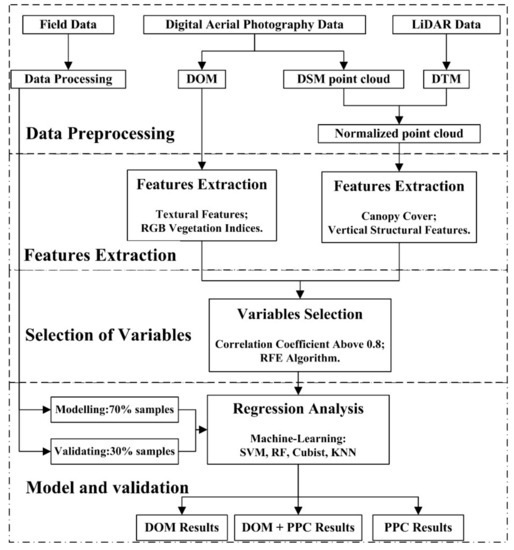
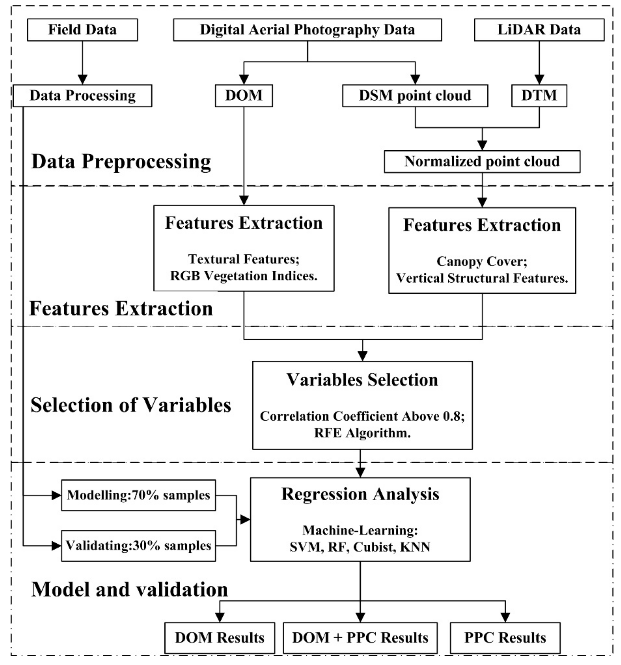
The research method consists of four parts: data preprocessing, features extraction, selection of the variables, and the model and validation (Figure 2).

Figure 2. Technical flow chart of the process of retrieving AGB and LAI.

2.3.1. LiDAR Data Pre-Processing

LiDAR data pre-processing was carried out by the CAF. This included noise removal of the point cloud and point cloud classification, which gives ground and non-ground echoes according to the proprietary algorithm implemented in the TerraScan software (https://www.terrasolid.com, TerraSolid Ltd., Helsinki, Finland). A digital terrain model (DTM) with a 1-m spatial resolution was derived using a triangulated irregular network (TIN) interpolating method from the ground-classified points.

2.3.2. DAP Data Pre-Processing

First, we combined an onboard inertial measurement unit (IMU)/global positioning system (GPS) with camera exposure position information and ground base station data of the closest official reference points of the Heilongjing Bureau of Surveying and Mapping Geoinformation to generate the accurate position and attitude information of every photo taken using DGPS. The overall accuracy was between 10 cm and 15 cm.

We used the SfM algorithm to generate a DSM dense point cloud and DOM from an overlapping collection of digital aerial photographs in the proprietary software Pix4DMapper Professional Edition 2.1.0 (64 bit) (https://pix4d.com/, Pix4D S.A. Lausanne, Switzerland). The resolution of the DOM is 0.1 m, and the tolerance of data processing is 0.02 m. SfM is the process of estimating the 3D structure of a scene from a set of 2D images. SfM requires point correspondences between images. Corresponding points were identified either by matching features or tracking points from image 1 to image 2 [43]. The fundamental matrix describes the epipolar geometry of two images and is computed using the corresponding points of two images. The orientation and location in the specified coordinate system are returned by relative and absolute orientation calculation. The 3D locations of matched points are determined using triangulation.

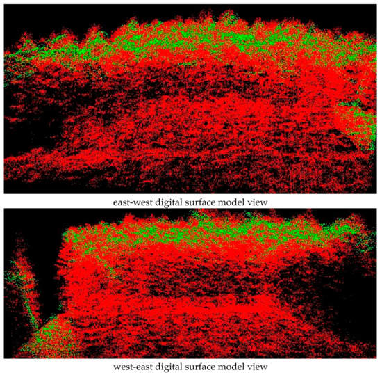
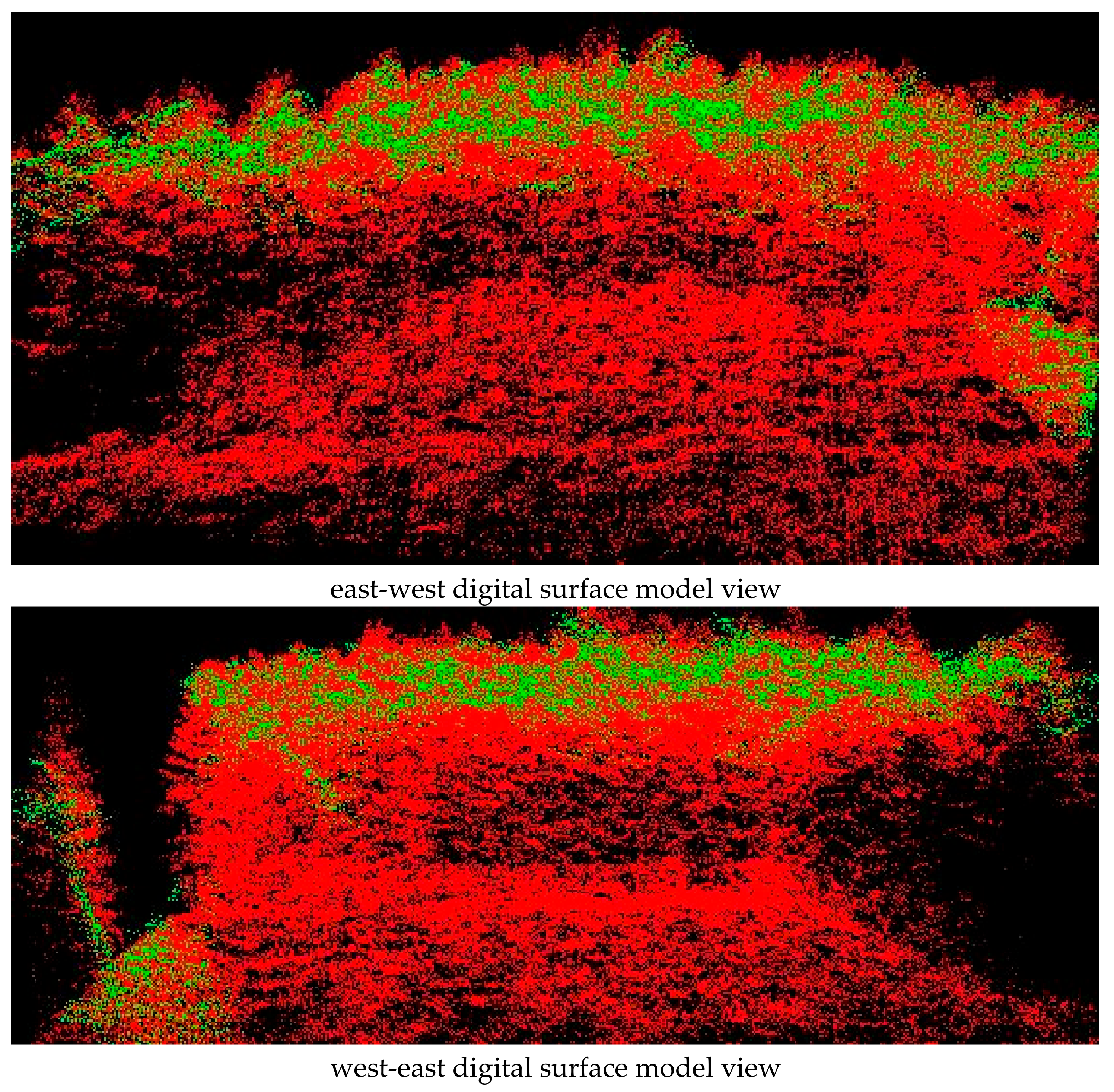
We compared the DSM point cloud from the DAP data to the DSM point cloud from the LiDAR data (Figure 3). The results showed that the average range deviation between the LiDAR point cloud and the DAP point cloud results was less than 0.5 m.

Figure 3. Matching the figures of the digital aerial photograph (DAP) point cloud and the light detection and ranging (LiDAR) point cloud. Red points are LiDAR point cloud and the green points are the DAP point cloud.

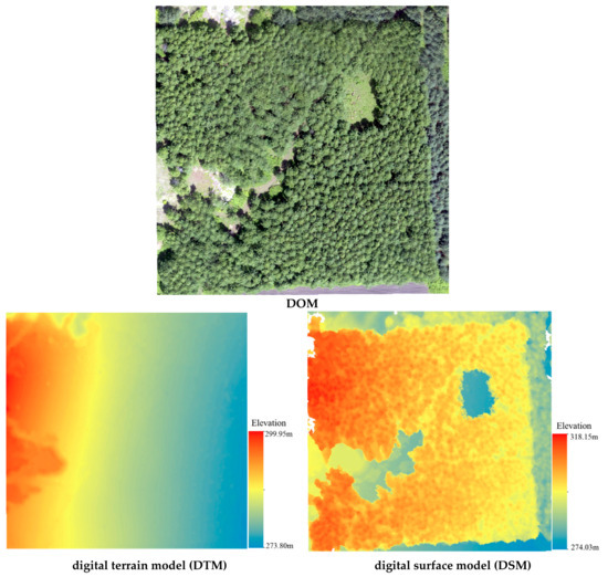
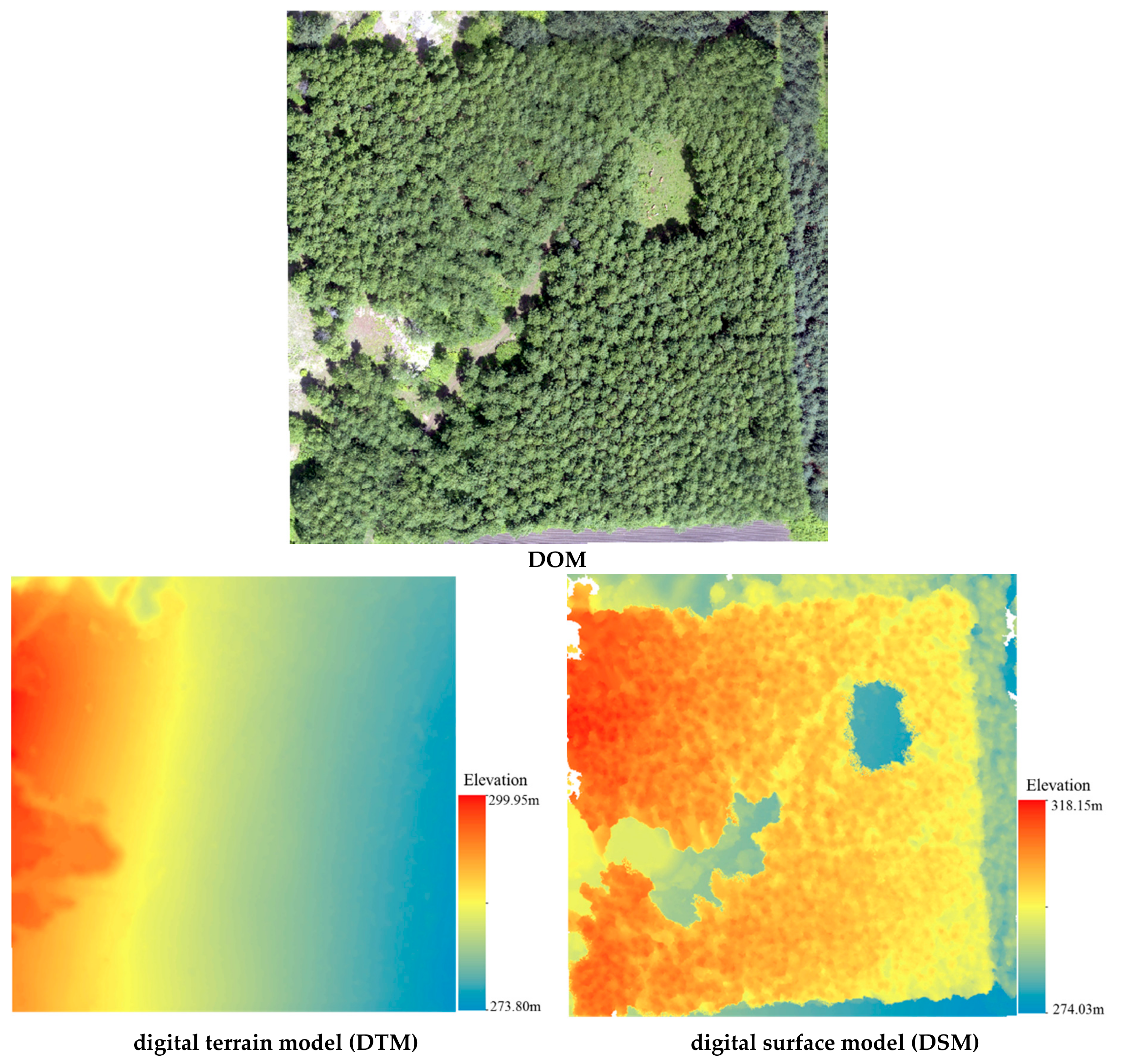
The results of DOM, DTM, and DSM in the same area are shown in Figure 4. Then, the DTM point cloud from LiDAR and the DSM point cloud from DAP were optimized in Terrascan software. The absolute heights of the point cloud were normalized by subtracting the terrain heights from DTM to obtain the relative heights.

Figure 4. Data pre-processing results of digital aerial photographs and LiDAR.

2.3.3. Feature Extraction of DOM

Feature extraction of DOM can be divided into two different categories of features: (1) RGB vegetation indices and (2) textural features.

RGB vegetation indices were constructed by imitating the structure of the NIR band from 0.1-m resolution DOM data. We used the digital number (DN) value to take the place of reflectance in this study (Table 6). Six kinds of vegetation indices were created using DN values of the red, green, and blue bands.

Table 6. Six vegetation indices of red-green-blue (RGB) bands.

Vegetation Indices Name	Equations 1	References
Visible differential vegetation index (VDVI)	$\frac{2\times {\mathrm{DN}}_{\mathrm{G}}-{\mathrm{DN}}_{\mathrm{R}}-{\mathrm{DN}}_{\mathrm{B}}}{2\times {\mathrm{DN}}_{\mathrm{G}}+{\mathrm{DN}}_{\mathrm{R}}+{\mathrm{DN}}_{\mathrm{B}}}$	[44]
Excess green index (EXG)	$2\times {\mathrm{DN}}_{\mathrm{G}}-{\mathrm{DN}}_{\mathrm{R}}-{\mathrm{DN}}_{\mathrm{B}}$	[44]
Visible atmospherically resistant index (VARI)	$\frac{{\mathrm{DN}}_{\mathrm{G}}-{\mathrm{DN}}_{\mathrm{R}}}{{\mathrm{DN}}_{\mathrm{G}}+{\mathrm{DN}}_{\mathrm{R}}-{\mathrm{DN}}_{\mathrm{B}}}$	[45]
Green red ratio index (GRRI)	$\frac{{\mathrm{DN}}_{\mathrm{G}}}{{\mathrm{DN}}_{\mathrm{R}}}$	[46]
Green blue ratio index (GBRI)	$\frac{{\mathrm{DN}}_{\mathrm{G}}}{{\mathrm{DN}}_{\mathrm{B}}}$	[47]
Red blue ratio index (RBRI)	$\frac{{\mathrm{DN}}_{\mathrm{R}}}{{\mathrm{DN}}_{\mathrm{B}}}$

¹ DN_G: digital number (DN) value of the green band. DN_R: digital number (DN) value of the red band. DN_B: digital number (DN) value of the blue band.

Four textural features (mean, homogeneity, dissimilarity, and correlation) were extracted from the first principal component of the 0.1-m DOM in this study (Table 7). Every feature includes four different window sizes of 4.5 m, 6.5 m, 10.1 m and 25.1 m.

Table 7. Four textural features.

Feature Name	Equations 1
Mean	${\displaystyle \sum }_{i,j=0}^{N-1}i{P}_{i,j}$
Homogeneity	${\displaystyle \sum }_{i,j=0}^{N-1}i\frac{P_{ij}}{1+{\left(i-j\right)}^2}$
Dissimilarity	${\displaystyle \sum }_{i,j=0}^{N-1}i{P}_{i,j}\left|i-j\right|$
Correlation	${\displaystyle \sum }_{i,j=0}^{N-1}i{P}_{i,j}\left[\frac{\left(i-mean\right)\left(j-mean\right)}{\sqrt{varianc{e}_{i}varianc{e}_j}}\right]$

¹ i is the line number of the gray level co-occurrence matrix. j is the column number of the gray level co-occurrence matrix. P_ij is normalized co-occurrence matrix. ME is the mean value of the gray level co-occurrence matrix. VA is the variance value of the gray level co-occurrence matrix.

The mean values of vegetation indices and textural features were calculated using R packages including caret [48], raster [49] and dplyr [50].

2.3.4. Feature Extraction of PPC

PPC is used to provide forest vertical structure parameters. Height statistics (standard deviation (Stddev), variance, coefficient of variation (CV), skewness, kurtosis, maximum, mean, mode, average absolute deviation (AAD), l-moments, canopy relief ratio, median of absolute deviation (MADMedian), and mode of absolute deviation (MADMode)), height percentiles (IQ, P50, P75, P95, and P100), coverage statistical features (percentage above mean, percentage above mode, percentage above 2 m, 10 to 20 proportion, and 5 to 10 proportion) (Table 8), and canopy cover (CC) were extracted based on relative height values from normalized point clouds in a hierarchical way, using open source FUSION software (http://forsys.cfr.washington.edu/fusion).

Table 8. Forest vertical structure parameters from the normalized point cloud.

Variable Type	Variable Name	Variable Description	References
Height statistics of point cloud	Stddev	Standard deviation of point cloud height	[51]
	Variance	Variance of point cloud
	CV	Coefficient of variation of point cloud height
	Skewness	Skewness of point cloud height	[52]
	Kurtosis	Kurtosis of point cloud height
	Maximum	Maximum of point cloud height	[51]
	Mean	Mean of point cloud height
	Mode	Mode of point cloud height
	AAD	Average absolute deviation
	L-moments	Linear moment, including L1,L2,L3,L4	[53]
	Canopy relief ratio	$\frac{\left(mean-min\right)}{\left(max-\min \right)}$	[54]
	MADMedian	Median of absolute deviation of point cloud above median
	MADMode	Mode of absolute deviation of point cloud above median
Height percentile of point cloud	IQ	Height 75th percentile minus 25th percentile	[51]
	P99	Height 99th percentile
	P95	Height 95th percentile
	P75	Height 75th percentile
	P50	Height 50th percentile
Coverage of point cloud	Percentage above mean	Percentage of point cloud above mean	[54]
	Percentage above mode	Percentage of point cloud above mode
	Percentage above 2 m	Percentage of point cloud above 2 m
	10 to 20 proportion	Proportion of point cloud from 10 and 20 m
	5 to 10 proportion	Proportion of point cloud from 5 and 10 m

CC is the index that describes the degree of canopy connection of trees, and it is the ratio of canopy projected area to woodland area. CC was generated from the normalized point cloud. We used the height threshold to distinguish between ground points and tree points.

2.3.5. Estimation of AGB and LAI

In the study, three types of data sources were used to estimate forest AGB and LAI. We merged all features from DOM, all structural variables from PPC, and a combination of both. Because there are four different texture window sizes, we need to separately merge all parameters. Because of high correlations among variables, the correlation was statistically calculated using R packages including caret [48] and corrplot [55]. We tested for multicollinearity between variables and removed variables with Pearson’s r > 0.8 to reduce the redundancy of variables. In AGB retrieval, 10 variables for DOM, 6 variables for PPC, and 16 variables for a combination of both were selected after removing redundant variables. In LAI retrieval, 10 variables for DOM, 10 variables for PPC, and 20 variables for a combination of both were selected after removing redundant variables (Table 9).

Table 9. Variables from DOM and PPC after reducing redundancy.

Variable Type		Variable Name
		LAI	AGB
PPC features	Height statistics	Stddev
		Variance
		CV
		Skewness	Mean
		Kurtosis	Canopy relief ratio
	Height percentile	IQ
		P95
	Coverage	Percentage above mean
		10 to 20 proportion
	Canopy cover	Mean(CC)
DOM features	Texture	Mean(mean)
		Mean(dissimilarity)
		Mean(homogeneity)
		Mean(correlation)
	Vegetation indices	Mean(VDVI)
		Mean(EXG)
		Mean(VARI)
		Mean(GRRI)
		Mean(GBRI)
		Mean(RBRI)

Random forest (RF) is a natural multiclass algorithm with an internal measure of feature importance. The random forest recursive feature elimination (RF-RFE) selection method is basically a recursive process that ranks features according to some measure of their importance [56].

According to the importance of variables and referring to the model accuracy of cross validation, the influence of each variable on the cross-validation accuracy of the model was considered iteratively from the most important variable to the least important one. Following a machine-learning (ML) regression analysis, the joint RF-RFE algorithm was carried out to estimate AGB and LAI based on DOM variables, PPC variables, and a combination of both. For each of the three data sources, we used four ML model algorithms: random forest (RF), supporting vector machine (SVM), k-nearest neighbor (KNN) and Cubist to build the model. The tuning methods of the four models and RF-RFE operation were achieved using R package, including caret [48], e1071 [57], cubist [58] and randomForest [59]. In the Cubist model, the value range of number parameter committees of model trees is from 1 to 50, with a step of 1. The range of the nearest-neighbor sample neighbors is from 0 to 9, with a step of 1. The tuneLength of mtry is 7 and ntree is 1000 in the RF model. The tuneLength of k in the KNN model is 50. The values of kernel function gamma are 0.5, 1, and 2. The values of the punish coefficient cost are 0.1, 1, 10, and 100.

For DOM and PPC alone, we chose the first half of all variables. For DOM + PPC, we chose the first third of total variables based on RFE results to participate in THE ML model. Thus, five variables of DOM, three variables of PPC and six variables of DOM + PPC were used in the estimation of AGB. Five variables of DOM, five variables of PPC, and seven variables of DOM + PPC were chosen in the estimation of LAI.

In total, 70% of samples (approximately 40 plots for AGB and approximately 135 plots for LAI) were randomly selected for training, and 30% of samples (approximately 16 plots for AGB and approximately 57 plots for LAI) were selected for validation in this study. For regression analysis, we ensured the distribution of different densities and different tree species plots in training and validation samples.

2.4. Model Accuracy Evaluation

After the regression model was established, the coefficient of determination, R-Square (R²), and root mean square error (RMSE) were used to assess the goodness and accuracy of the established models. The larger the R² value, and the stronger correlation. The smaller the RMSE value, the higher the predicted accuracy. R² and RMSE were calculated using Equations (1) and (2).

$$R^2=1-\frac{{{\displaystyle \sum }}_{i=1}^n{\left(y_i-y_i^{\prime }\right)}^2}{{{\displaystyle \sum }}_{i=1}^n{\left(y_i-\overline{y_i}\right)}^2}$$

(1)

$$RMSE= \sqrt{\frac{{{\displaystyle \sum }}_{i=1}^n{\left(y_i-y_i^{\prime }\right)}^2}{n}}$$

(2)

where n is the number of plots, $y_i$is the ground field measurement reference value of AGB or LAI for plot i; $\overline{y_i}$ is the average value of $y_i$; $y_i^{\prime }$ is the model estimate value of AGB or LAI.

3. Results

About 70% of plot measurements were used to build the regression analysis model, and 30% were retained to validate the model. By training and comparing AGB and LAI retrieval results based on textural features of four window sizes using same method, we chose features of 6.5 m window size to retrieve AGB and LAI. The tuning results of four machine-learning models for the estimation of AGB and LAI from the three data sources are shown in Table 10.

Table 10. The best combination of parameters for the four models for the estimation of AGB and LAI.

Models	AGB			LAI
	DOM	PPC	DOM + PPC	DOM	PPC	DOM + PPC
Cubist 1	c = 2, n = 2	c = 45, n = 9	c = 2, n = 2	c = 8, n = 2	c = 6, n = 9	c = 11, n = 2
KNN	k = 5	k = 11	k = 5	k = 7	k = 11	k = 5
RF	mtry = 4	mtry = 3	mtry = 2	mtry = 2	mtry = 3	mtry = 3
SVM 2	g = 2, c = 100	g = 0.5, c = 100	g = 0.5, c = 1	g = 1, c = 1	g = 1, c = 1	g = 0.5, c = 1

¹ c: committees, n: neighbors. ² g: gamma, c: cost.

The variables used for final modeling are shown in Table 11, ranked according to the importance.

Table 11. The variables used in modeling.

Importance	AGB
	DOM	PPC	DOM + PPC
1	VDVI	P95	P95
2	RBRI	Mean	P-Mean 1
3	EXG	10 to 20 proportion	10 to 20 proportion
4	Mean		D-Mean 2
5	GBRI		VDVI
6			CC
Importance	LAI
	DOM	PPC	DOM + PPC
1	GRRI	CC	CC
2	Mean	P95	GRRI
3	VARI	10 to 20 proportion	P95
4	VDVI	CV	10 to 20 proportion
5	EXG	Skewness	D-Mean 2
6			VARI
7			VDVI

¹ P-Mean: mean of point cloud height. ² D-Mean: the textural feature from DOM.

As we can see from Table 11, vegetation indices are the most significant variables for the estimation of AGB in models obtained using DOM data. In addition, the texture mean variable is important. In those models comprising only PPC variables, height percentile and statistic are the most significant variables. Concerning DOM + PPC variables, height and coverage variables are the most significant variables; texture and vegetation index variables followed.

For estimation of LAI, the green red ratio index (GRRI) is the most significant variable in DOM models; the texture mean variable followed. In PPC models, coverage and height percentile are the most significant variables. In the combined DOM + PPC variables, the coverage variable is the most significant, followed by the vegetation index variable.

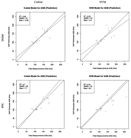
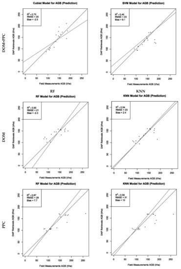
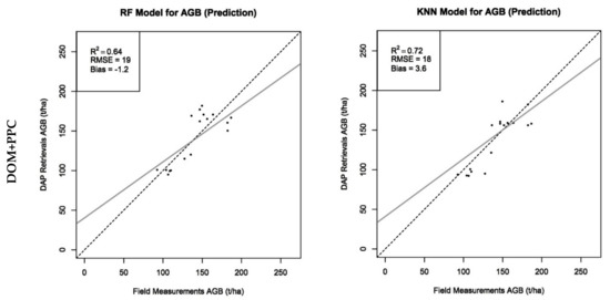
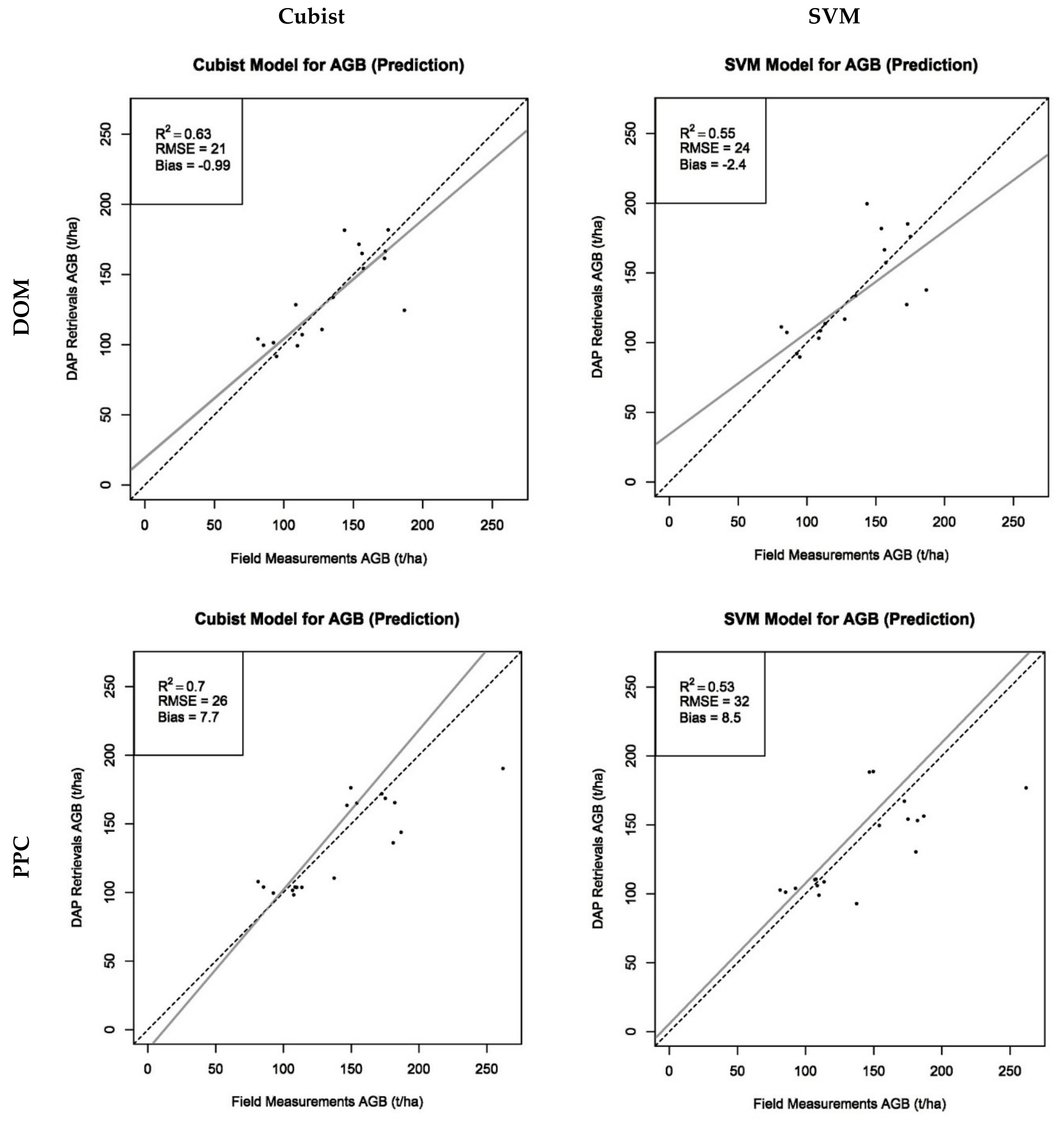
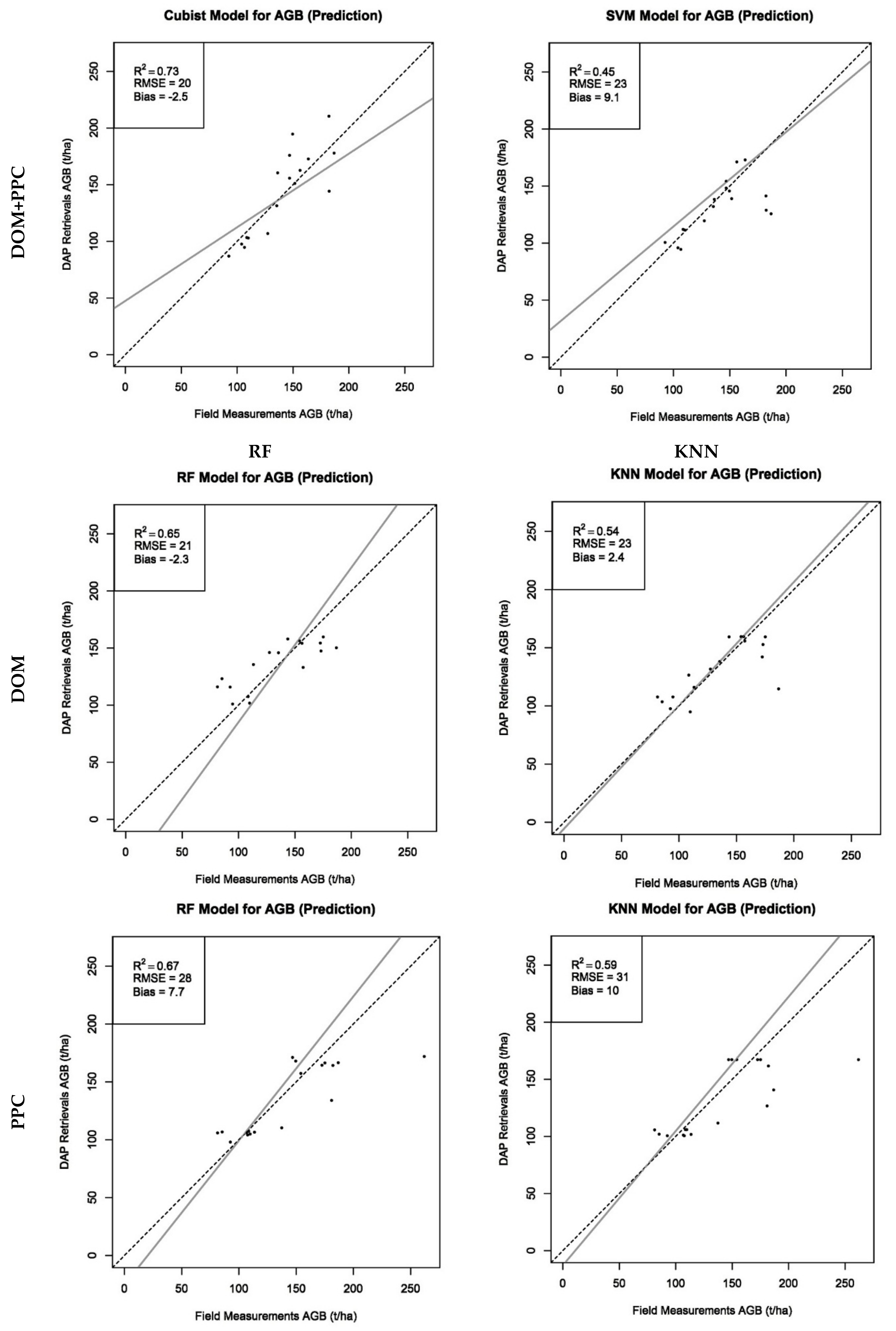
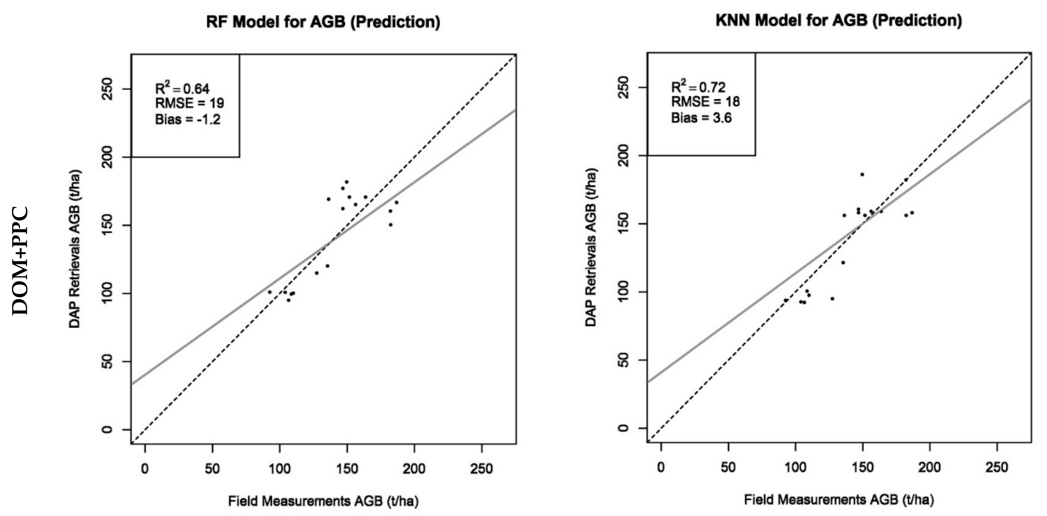
As we can see from Figure 5, for field data versus estimated data in the estimation of AGB, the optimal values of R² and RMSE in DOM alone are 0.65 and 21 t/ha, respectively. In PPC alone, the optimal values are 0.7 and 26 t/ha. In DOM + PPC, the values are 0.73 and 20 t/ha, respectively. The results obtained using a combination of DOM and PPC provide increased R² accuracy. DOM results are particularly poor.

Figure 5. Prediction accuracy of the four models for AGB estimation based on the three sources of data.

It is worth noting that the differences between PPC and DOM + PPC models are less marked. In some cases, PPC variables alone provide better results. It is apparent that R² is much smaller for the model based only on DOM variables compared to the two others. PPC and DOM + PPC models provide very similar results.

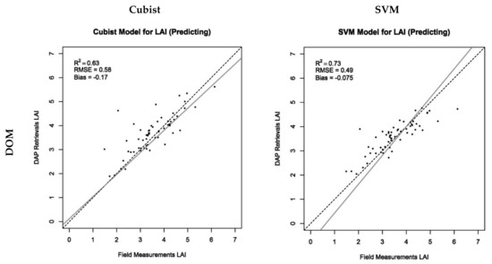
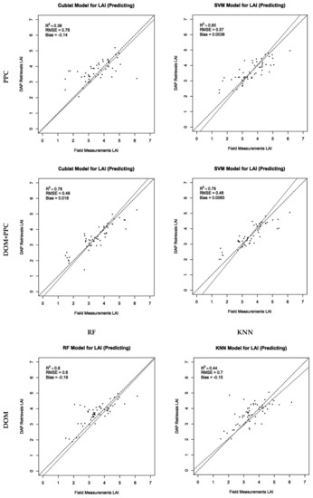
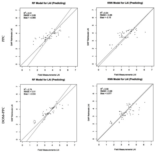
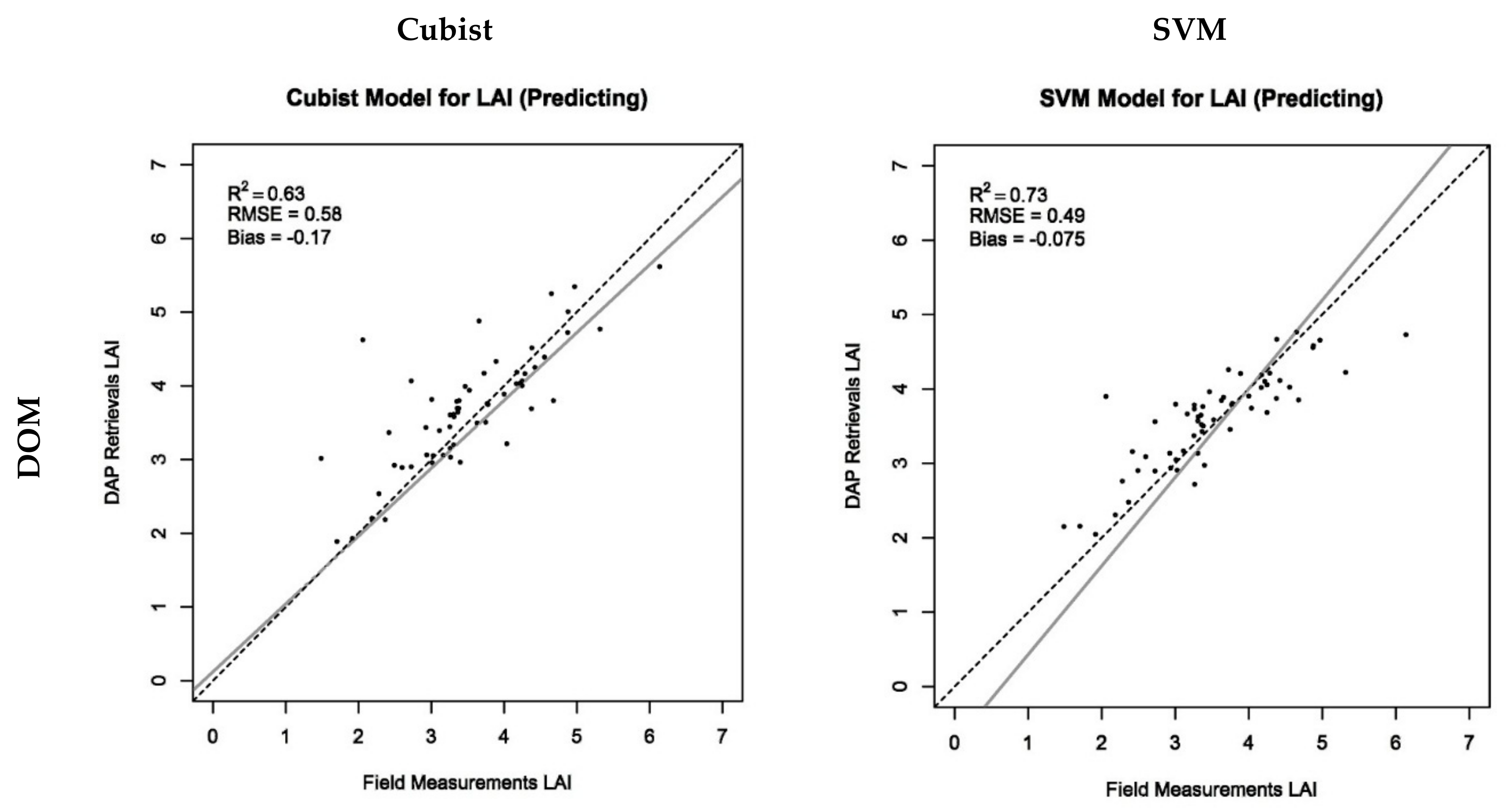
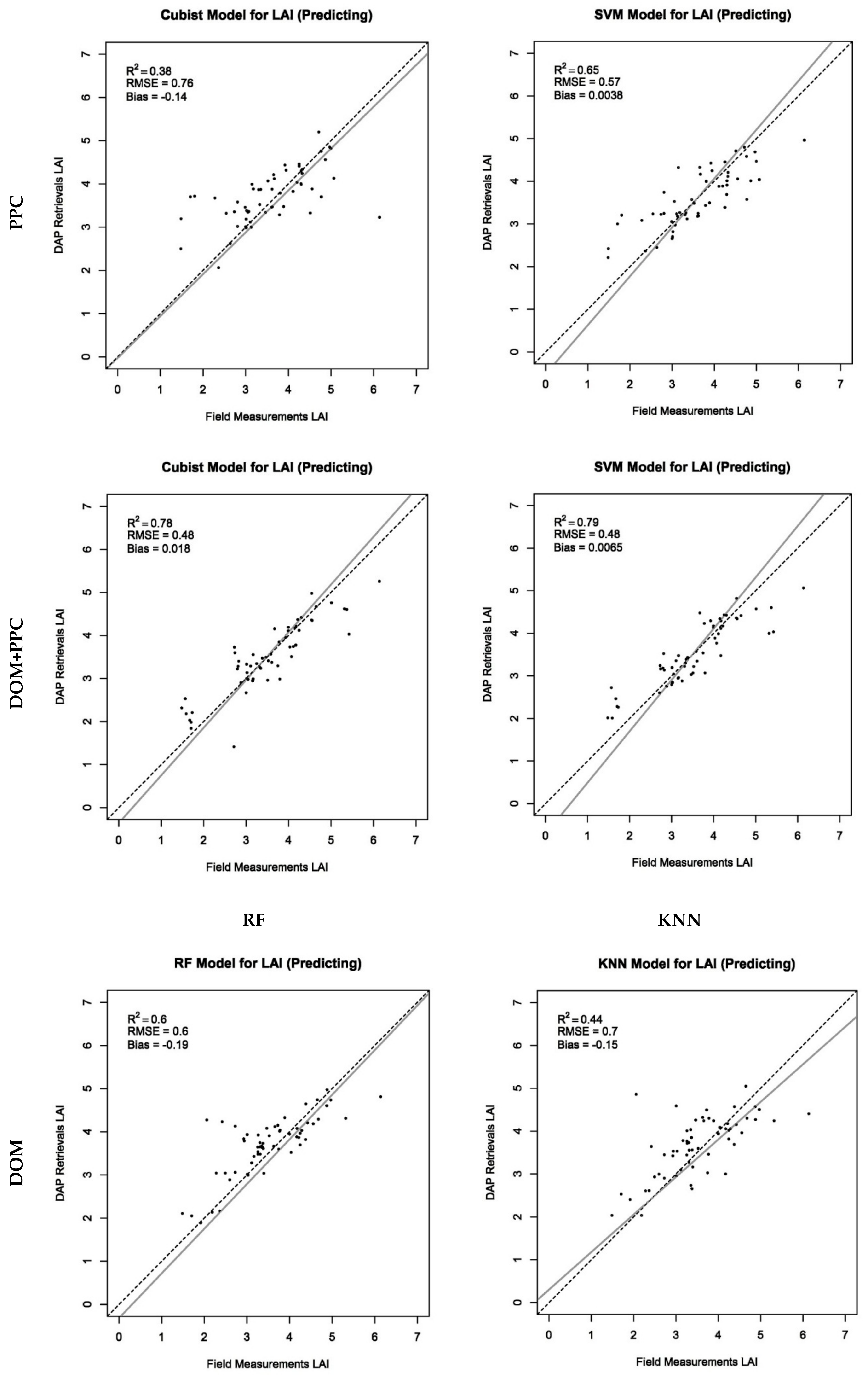
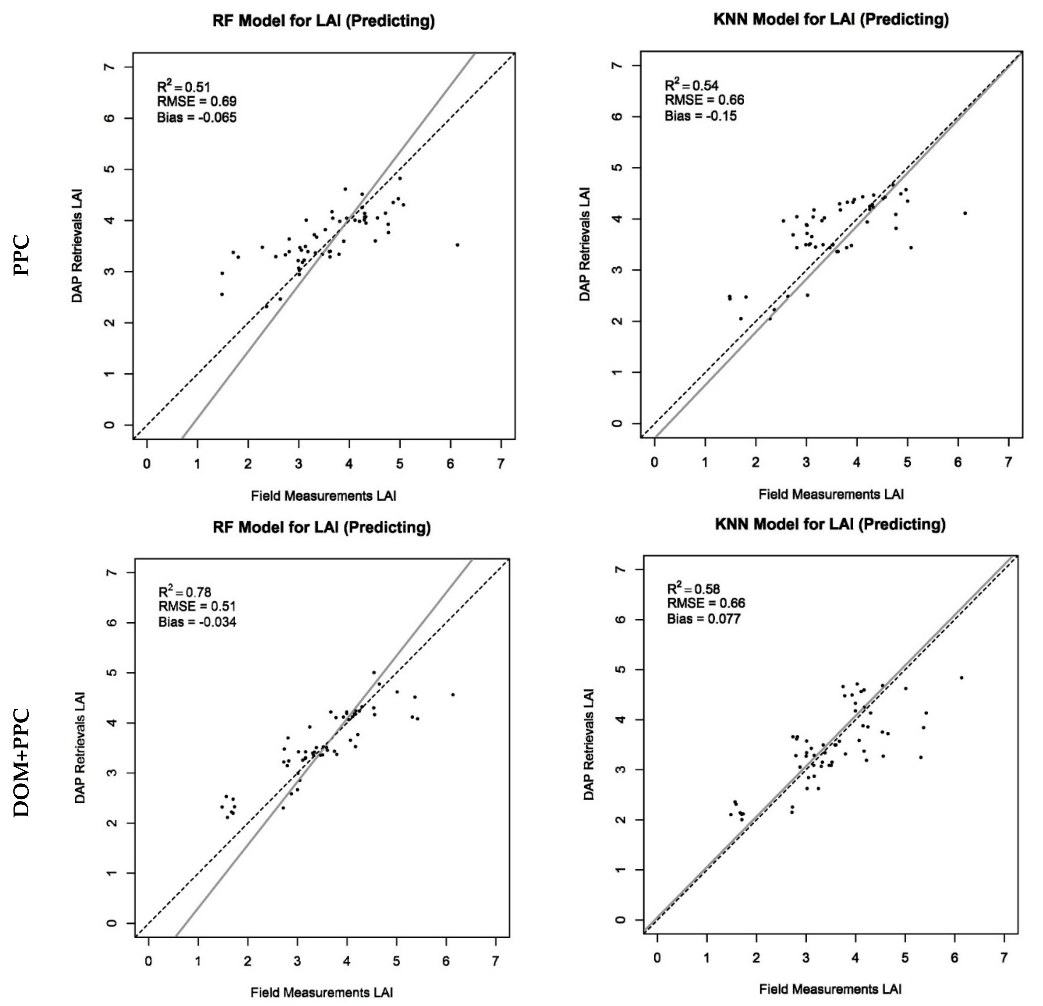
The field data versus the estimated data in the estimation of LAI are shown in Figure 6. The values of R² and RMSE in DOM alone are 0.73 and 0.49, respectively. In PPC alone, the values are 0.65 and 0.57, respectively. In DOM + PPC, the values are 0.79 and 0.48, respectively. The results obtained using the combination of DOM and PPC provide increased R² accuracy. PPC results are particularly poor.

Figure 6. Prediction accuracy of the four models for LAI retrieval based on the three data sources.

The differences between DOM and DOM + PPC models are less marked. DOM variables alone provide better results. It is apparent that R² is much smaller for the model based only on PPC variables compared to the two other models. In particular, DOM and DOM + PPC models provide very similar results.

4. Discussion

As important ecological and biophysical parameters, AGB and LAI were estimated using three data sources (DOM data alone, PPC data alone, and DOM + PPC data) from the DAP data in this study. Our findings showed that combining DOM and PPC data could improve estimation accuracy for AGB and LAI.

Better accuracy (R² = 0.73 and RMSE = 20 t/ha) for the AGB estimation based on a Cubist regression model was achieved from the combined model processing of vertical structure, vegetation indices, and textural features from the combination of DOM and PPC data. The retrieval result of AGB from height variables of PPC data was better than the textural feature and vegetation indices from DOM data. Height and coverage variables derived from PPC data were the first three selections. This shows that height is a key parameter in the estimation of AGB. Studies using airborne LiDAR or a combination of LiDAR and aerial photographs have shown how height can be used to estimate AGB [4,37,60]. Our study has confirmed that height is particularly important and a suitable index to AGB estimation when we used photogrammetric point cloud from the results of SfM approach processing. Ota et al. [37] obtained aboveground biomass using aerial photographs in a seasonal tropical forest. Canopy height models from aerial photograph DSM and LiDAR DTM yielded higher accuracy (R² = 0.93). Hansen et al. [61] estimated forest biomass based on empirical relationships between field-observed biomass and variables derived from LiDAR data, and a relatively lower accuracy was obtained (R² = 0.71, RMSE = 158 Mg/ha). Our accuracy of AGB estimation from combined DOM and PPC data is between Ota’s and Hansen’s results.

The R² and RMSE values of LAI estimation based on the SVM regression model from the combined DOM and PPC data were 0.79 and 0.48, respectively. Canopy cover (CC) from PPC data and the green red ratio index (GRRI) from DOM data contributed better results. It is worth noting that the GRRI is the second most important variable after CC. This indicates that GRRI has a strong contribution to LAI estimation. Previous studies using LiDAR, satellite images, or a combination of both showed similar results in estimating LAI. Ma et al. [62] estimated LAI based on full-waveform LiDAR data using a radiative transfer model. The R² and RMSE values of estimated LAI were 0.73 and 0.67, respectively. Mathews et al. [35] used a stepwise regression model to predict LAI based on a high-density point cloud using unmanned aerial vehicle (UAV) collection. The final result of the R² value was 0.57. Omer et al. [63] used spectral vegetation indices calculated from WorldView-2 data to predict LAI at the tree species level using support vector machines and artificial neural networks machine learning regression algorithms. They obtained better accuracy (R² = 0.75, RMSE = 0.05). Ma et al. [23] used the canopy height variable from LiDAR and the BRDF/Albedo variable from MODIS optical data to estimate LAI. The highest R² value was 0.73. Our accuracy is slightly higher than previous study results, and our study has confirmed that canopy coverage and vegetation index are particularly important and suitable indices to LAI estimation.

Compared with PPC data, DOM data had lower estimation accuracy (R² = 0.65, RMSE = 21 t/ha) of AGB, but the estimation accuracy (R² = 0.73, RMSE = 0.49) of LAI was higher. Similar findings were reported [9,63]. Summarizing these results above, we believe that the spectral and textural features had a larger contribution to LAI retrieval than vertical height features, and the forest vertical height features had greater effects on AGB retrieval. Our study is slightly different from previous studies. The differences are mainly because of the different data sources, different types of vegetation, biomass abundance, and canopy density.

As we can see in Figure 5 and Figure 6, a combination of DOM and PPC data could improve the estimation accuracy of AGB and LAI compared with either data source alone. The combined DOM and PPC data yielded the highest estimation accuracy for AGB (R² = 0.73, RMSE = 20 t/ha) and LAI (R² = 0.79, RMSE = 0.48). These estimations were made using machine-learning with the Cubist regression model and SVM regression model, respectively. Our study has demonstrated the ability to estimate AGB and LAI using the combination of DOM and PPC from DAP data with the SfM approach.

The results of our study using only DAP data are consistent with previous studies using LiDAR and other optical remote sensing data. However, the acquisition and processing cost of DAP data is much lower than that of LiDAR, while the spatial resolution is much higher than that of optical remote sensing data. Using DAP data to estimate forest parameters is worthy of further exploration and research. Our study could provide valuable guidance for accurate AGB and LAI estimation using DOM+PPC data from DAP in boreal coniferous forests.

In this study, with the exception of DEM from LiDAR data, we used DAP data alone with only red, green, and blue visible bands to estimate AGB and LAI. In previous studies, multispectral vegetation indices were used [63]. The near-infrared band can provide much better information about vegetation health [64]. We imitated the principle of multispectral vegetation indices to construct visible light vegetation indices. The results may have been improved if we added the spectral information of the near-infrared band. This work will be performed in a future study.

For a future practical application of the results from this study in other areas, we can consider all variables (vertical features and horizontal features) in this paper as realistic approaches.

5. Conclusions

The objective of this study is to explore the ability of retrieving forest parameters only using DOM, PPC, and DOM+PPC from RGB-only DAP data. In the paper, three analyses on DOM, PPC, and combined DOM and PPC data for the estimation of AGB and LAI have been presented. The study indicates that a combination of DOM and PPC data is useful as it provides a slight increase in estimation accuracy. Height and coverage variables of PPC, texture mean value, and visible differential vegetation index (VDVI) of DOM are significantly related to the estimation of AGB (R² = 0.73, RMSE = 20 t/ha). The canopy cover of PPC and green red ratio index (GRRI) of DOM are the most strongly related to the estimation of LAI, followed by the height and coverage variables of PPC, texture mean value, the visible atmospherically resistant index (VARI), and the VDVI of DOM (R² = 0.79, RMSE = 0.48). The model derived from only DOM data provides lower accuracy than only PPC data for the estimation of AGB at the Mengjiagang forest farm. In terms of LAI estimation, the result is different. Variables from either DOM or PPC data alone can provide the majority of the explanatory contribution for LAI estimation.

The current study focuses on boreal coniferous forest areas using RGB-only DAP data, with an R2 higher than 0.7. Nevertheless, more studies should be carried on a variety of forest types to determine the validity of the defined parameters and the accuracy reported. Possible future developments of this work are (1) to consider other target variables (such as tree height and individual tree segment), (2) to use the same method in temperate broadleaved forest areas to determine the universality of the method, and (3) to add NIR spectral information.

References

- Dubayah, R.O.; Drake, J.B. Lidar remote sensing for forestry. J. For. 2000, 98, 44–46. [Google Scholar]
- Ediriweera, S.; Pathirana, S.; Danaher, T.; Nichols, D. Estimating above-ground biomass by fusion of LiDAR and multispectral data in subtropical woody plant communities in topographically complex terrain in North-Eastern Australia. J. For. Res. 2014, 25, 761–771. [Google Scholar] [CrossRef] [Scilit]
- Næsset, E.; Gobakken, T.; Bollandsås, O.M.; Gregoire, T.G.; Nelson, R.; Ståhl, G. Comparison of precision of biomass estimates in regional field sample surveys and airborne LiDAR-assisted surveys in Hedmark County, Norway. Remote Sens. Environ. 2013, 130, 108–120. [Google Scholar] [CrossRef] [Scilit]
- Tuominen, S.; Haapanen, R. Estimation of forest biomass by means of genetic algorithm-based optimization of airborne laser scanning and digital aerial photograph features. Silva Fennica. 2013, 47, 20. [Google Scholar] [CrossRef] [Scilit]
- Chen, J.M.; Cihlar, J. Retrieving leaf area index of boreal conifer forests using Landsat TM images. Remote Sens. Environ. 1996, 55, 179–193. [Google Scholar] [CrossRef] [Scilit]
- Homolová, L.; Malenovský, Z.; Clevers, J.G.; García-Santos, G.; Schaepman, M.E. Review of optical-based remote sensing for plant trait mapping. Ecol. Complex. 2013, 15, 1–16. [Google Scholar] [CrossRef] [Scilit]
- Seidel, D.; Fleck, S.; Leuschner, C.; Hammett, T. Review of ground-based methods to measure the distribution of biomass in forest canopies. Ann. For. Sci. 2011, 68, 225–244. [Google Scholar] [CrossRef] [Scilit]
- Huang, J.L.; Ju, W.M.; Zheng, G.; Kang, T.T. Estimation of forest aboveground biomass using high spatial resolution remote sensing imagery. Acta Ecol. Sin. 2013, 33, 6497–6508. [Google Scholar] [CrossRef] [Scilit]
- Nichol, J.E.; Sarker, M.L.R. Improved biomass estimation using the texture parameters of two high-resolution optical sensors. IEEE Trans. Geosci. Remote Sens. 2011, 49, 930–948. [Google Scholar] [CrossRef] [Scilit]
- Gallaun, H.; Zanchi, G.; Nabuurs, G.J.; Hengeveld, G.; Schardt, M.; Verkerk, P.J. EU-wide maps of growing stock and above-ground biomass in forests based on remote sensing and field measurements. For. Ecol. Manag. 2010, 260, 252–261. [Google Scholar] [CrossRef] [Scilit]
- Gao, S.; Niu, Z.; Huang, N.; Hou, X. Estimating the Leaf Area Index, height and biomass of maize using HJ-1 and RADARSAT-2. Int. J. Appl. Earth Observ. Geoinf. 2013, 24, 1–8. [Google Scholar] [CrossRef] [Scilit]
- Mitchard, E.T.A.; Saatchi, S.S.; Woodhouse, I.H.; Nangendo, G.; Ribeiro, N.S.; Williams, M.; Ryan, C.M.; Lewis, S.L.; Feldpausch, T.R.; Meir, P. Using satellite radar backscatter to predict above-ground woody biomass: A consistent relationship across four different African landscapes. Geophys. Res. Lett. 2009, 36, L23401. [Google Scholar] [CrossRef] [Scilit]
- Greaves, H.E.; Vierling, L.A.; Eitel, J.U.H. Estimating aboveground biomass and leaf area of low-stature Arctic shrubs with terrestrial LiDAR. Remote Sens. Environ. 2015, 164, 26–35. [Google Scholar] [CrossRef] [Scilit]
- Moskal, M.L.; Zheng, G. Retrieving forest inventory variables with terrestrial laser scanning (TLS) in urban heterogeneous forest. Remote Sens. 2011, 4, 1–20. [Google Scholar] [CrossRef] [Scilit]
- Lin, Y.; Herold, M. Tree species classification based on explicit tree structure feature parameters derived from static terrestrial laser scanning data. Agric. For. Meteorol. 2015, 201, 710–711. [Google Scholar] [CrossRef] [Scilit]
- Tang, H.; Brolly, M.; Zhao, F.; Strahler, A.H.; Schaaf, C.L. Deriving and validating leaf area index (LAI) at multiple spatial scales through lidar remote sensing: A case study in Sierra National Forest, CA. Remote Sens. Environ. 2014, 143, 131–141. [Google Scholar] [CrossRef] [Scilit]
- Xing, Y.Q.; Huo, D.; You, H.T.; Tian, X.; Jiao, Y.T. Estimation of birch forest LAI based on single laser penetration index of airborne LiDAR data. J. Appl. Ecol. 2016, 27, 3469–3478. (In Chinese) [Google Scholar]
- Kankare, V.; Raty, M.; Yu, X.; Holopainen, M.; Vastaranta, M. Single tree biomass modeling using airborne laser scanning. ISPRS J. Photogramm. Remote Sens. 2013, 85, 66–73. [Google Scholar] [CrossRef] [Scilit]
- Lefsky, M.A.; Cohen, W.B.; Parker, G.G.; Harding, D.J. LiDAR remote sensing for ecosystem studies. BioScience 2002, 52, 19–30. [Google Scholar] [CrossRef] [Scilit]
- Lu, D. The potential and challenge of remote sensing-based biomass estimation. Int. J. Remote Sens. 2006, 27, 1297–1328. [Google Scholar] [CrossRef] [Scilit]
- Ranson, K.J.; Sun, G.; Lang, R.H.; Chauhan, N.S.; Cacciola, R.J.; Kilic, O. Mapping of boreal forest biomass from spaceborne synthetic aperture radar. J. Geophys. Res. 1997, 102, 29599–29610. [Google Scholar] [CrossRef] [Scilit]
- Liu, L.X.; Coops, N.C.; Aven, N.W.; Pang, Y. Mapping urban tree species using integrated airborne hyper-spectral and LiDAR remote sensing data. Remote Sens. Environ. 2017, 200, 170–182. [Google Scholar] [CrossRef] [Scilit]
- Ma, H.; Song, J.L.; Wang, J.D.; Fu, D. Improvement of spatially continuous forest LAI retrieval by integration of discrete airborne LiDAR and remote sensing multi-angle optical data. Agric. For. Meteorol. 2014, 189, 60–70. [Google Scholar] [CrossRef] [Scilit]
- Zolkos, S.G.; Goetz, S.J.; Dubayah, R. A meta-analysis of terrestrial aboveground biomass estimation using LiDAR remote sensing. Remote Sens. Environ. 2013, 128, 289–298. [Google Scholar] [CrossRef] [Scilit]
- Luo, S.Z.; Wang, C.; Xi, X.H.; Pan, F.F.; Peng, D.L.; Zou, J.; Nie, S.; Qin, H.M. Fusion of airborne LiDAR data and hyperspectral imagery for aboveground and belowground forest biomass estimation. Ecol. Indic. 2017, 73, 378–387. [Google Scholar] [CrossRef] [Scilit]
- Tonolli, S.; Dalponte, M.; Neteler, M.; Rodeghiero, M.; Vescovo, L.; Gianelle, D. Fusion of airborne LiDAR and satellite multispectral data for the estimation of timber volume in the southern Alps. Remote Sens. Environ. 2011, 115, 2486–2498. [Google Scholar] [CrossRef] [Scilit]
- Tsui, O.W.; Coops, N.C.; Wulder, M.A.; Marshall, P.L.; McCardle, A. Using multi-frequency radar and discrete-return LiDAR measurements to estimate above-ground biomass and biomass components in a coastal temperate forest. ISPRS J. Photogramm. Remote Sens. 2012, 69, 121–133. [Google Scholar] [CrossRef] [Scilit]
- Vaglio, L.G.; Chen, Q.; Lindsell, J.A.; Coomes, D.A.; Frate, F.D.; Guerriero, L.; Pirotti, F.; Valentini, R. Above ground biomass estimation in an African tropical forest with LiDAR and hyperspectral data. ISPRS J. Photogramm. Remote Sens. 2014, 89, 49–58. [Google Scholar] [CrossRef] [Scilit]
- Pflugmacher, D.; Cohen, W.B.; Kennedy, R.E.; Yang, Z. Using Landsat-derived disturbance and recovery history and Lidar to map forest biomass dynamics. Remote Sens. Environ. 2014, 151, 124–137. [Google Scholar] [CrossRef] [Scilit]
- Tuominen, S.; Pekkarinen, A. Performance of different spectral and textural aerial photograph features in multisource forest inventory. Remote Sens. Environ. 2005, 94, 256–268. [Google Scholar] [CrossRef] [Scilit]
- Puliti, S.; Ørka, H.O.; Gobakken, T.; Næsset, E. Inventory of small forest areas using an unmanned aerial system. Remote Sens. 2015, 7, 9632–9654. [Google Scholar] [CrossRef] [Scilit]
- Zahawi, R.A.; Dandois, J.P.; Holl, K.D.; Nadwodny, D.; Reid, J.L.; Ellis, E.C. Using lightweight unmanned aerial vehicles to monitor tropical forest recovery. Biol. Conserv. 2015, 186, 287–295. [Google Scholar] [CrossRef] [Scilit]
- Puliti, S.; Gobakken, T.; Ørka, H.O.; Næsset, E. Assessing 3D point clouds from aerial photographs for species-specific forest inventories. Scand. J. For. Res. 2017, 32, 68–79. [Google Scholar] [CrossRef] [Scilit]
- Nurminen, K.; Karjalainen, M.; Yu, X.W.; Hyyppä, J.; Honkavaara, E. Performance of dense digital surface models based on image matching in the estimation of plot-level forest variables. ISPRS J. Photogram. Remote Sens. 2013, 83, 104–115. [Google Scholar] [CrossRef] [Scilit]
- Mathews, A.J.; Jensen, J.L.R. Visualizing and quantifying vineyard canopy LAI using an unmanned aerial vehicle (UAV) collected high density structure from motion point cloud. Remote Sens. 2013, 5, 2164–2183. [Google Scholar] [CrossRef] [Scilit]
- Dandois, J.P.; Ellise, E.C. High spatial resolution three-dimensional mapping of vegetation spectral dynamics using computer vision. Remote Sens. Environ. 2013, 136, 259–276. [Google Scholar] [CrossRef] [Scilit]
- Ota, T.; Ogawa, M.; Shimizu, K.; Kajisa, T.; Mizoue, N. Aboveground biomass estimation using structure from motion approach with aerial photographs in a seasonal tropical forest. Forests 2015, 6, 3883–3898. [Google Scholar] [CrossRef] [Scilit]
- Fonstad, M.A.; Dietrich, J.T.; Courville, B.C; Jensen, J.L; Carbonneau, P.E. Topographic structure from motion: A new development in photogrammetric measurement. Earth Surf. Process. Landf. 2013, 38, 421–430. [Google Scholar] [CrossRef] [Scilit]
- Asner, G.P.; Sinan, S.; Knapp, D.E.; Selmants, P.C.; Martin, R.E.; Hughes, R.F.; Giardina, C.P. Rapid forest carbon assessments of oceanic islands: A case study of the Hawaiian archipelago. Carbon Balance Manag. 2016, 11, 1–13. [Google Scholar] [CrossRef] [Scilit] [PubMed]
- Tamm, T.; Remm, K. Estimating the parameters of forest inventory using machine learning and the reduction of remote sensing features. Int. J. Appl. Earth Obs. 2009, 11, 290–297. [Google Scholar] [CrossRef] [Scilit]
- Li, H.K.; Lei, Y.C. China Forest Vegetation Biomass and Carbon Stock Assessment; China Forestry Publishing House: Beijing, China, 2010. (In Chinese) [Google Scholar]
- Chen, C.G.; Zhu, J.F. Northeast Main Forest Biomass Handbook; China Forestry Publishing House: Beijing, China, 1989. (In Chinese) [Google Scholar]
- MathWorks. Structure from Motion. Available online: http://www.mathworks.com/help/vision/ug/structure-from-motion.html (accessed on 4 May 2018).
- Torres-Sánchez, J.; Peña, J.M.; Castro, A.I.; López-Granados, F. Multi-temporal mapping of the vegetation fraction in early-season wheat fields using images from UAV. Comput. Electron. Agric. 2014, 103, 104–113. [Google Scholar] [CrossRef] [Scilit]
- Gitelson, A.A.; Vina, A.; Arkebauer, T.J.; Rundquist, D.C.; Keydan, G.P.; Leavitt, B.; Keydan, G. Remote estimation of leaf area index and green leaf biomass in maize canopies. Geophys. Res. Lett. 2003, 30, 335–343. [Google Scholar] [CrossRef] [Scilit]
- Verrelst, J.; Schaepman, M.E.; Koetz, B.; Kneubuhler, M. Angular sensitivity analysis of vegetation indices derived from CHRIS/PROBA data. Remote Sens. Environ. 2008, 112, 2341–2353. [Google Scholar] [CrossRef] [Scilit]
- Sellaro, R.; Crepy, M.; Trupkin, S.A.; Karayekov, E.; Buchovsky, A.S.; Rossi, C.; Casal, J.J. Cryptochrome as a sensor of the blue/green ratio of natural radiation in Arabidopsis. Plant Physiol. 2010, 154, 401–409. [Google Scholar] [CrossRef] [Scilit] [PubMed]
- Kuhn, M.; Weston, S.; Williams, A.; Keefer, C.; Engelhardt, A.; Cooper, T.; Mayer, Z.; Kenkel, B.; the R Core Team; Benesty, M.; et al. Caret: Classification and Regression Training. R Package Version 6.0-78. Available online: http://CRAN.R-project.org/package=caret (accessed on 1 August 2017).
- Hijmans, R.J. Raster: Geographic Data Analysis and Modeling R Package Version 2.6-7. 2017. Available online: https://CRAN.R-project.org/package=raster (accessed on 1 August 2017).
- Wickham, H.; Francois, R.; Henry, L.; Müller, K. Dplyr: A Grammar of Data Manipulation. R Package Version 0.7.4. 2017. Available online: https://CRAN.R-project.org/package=dplyr (accessed on 1 August 2017).
- Xycoon. Statistics-Econometrics-Forecasting. Office for Research Development and Education. Available online: http://www.xycoon.com (accessed on 2 April 2018).
- Engineering Statistics Handbook. Available online: http://www.itl.nist.gov/div898/handbook/eda/section3/eda35b.htm (accessed on 2 April 2018).
- Wang, O.J. Direct sample estimators of L moments. Water Resour. Res. 1996, 32, 3617–3619. [Google Scholar] [CrossRef] [Scilit]
- McGaughey, R.J. FUSION/LDV: Software for LiDAR Data Analysis and Visualization; FUSION Version 3.60+; United States Department of Agriculture: Washington, DC, USA, 2016. [Google Scholar]
- Wei, T.Y.; Simko, V. R package “corrplot”: Visualization of a Correlation Matrix (Version 0.84). 2017. Available online: https://github.com/taiyun/corrplot (accessed on 3 August 2017).
- Granitto, P.M.; Furlanello, C.; Biasioli, F.; Gasperi, F. Recursive feature elimination with random forest for PTR-MS analysis of agroindustrial products. Chemometr. Intell. Lab. 2006, 83, 83–90. [Google Scholar] [CrossRef] [Scilit]
- Meyer, D.; Dimitriadou, E.; Hornik, K.; Weingessel, A.; Friedrich Leisch, F. e1071: Misc Functions of the Department of Statistics, Probability Theory Group (Formerly: E1071), TU Wien. R package version 1.6-8. 2017. Available online: https://CRAN.R-project.org/package=e1071 (accessed on 3 August 2017).
- Kuhn, M.; Quinlan, R. Cubist: Rule- And Instance-Based Regression Modeling. R Package Version 0.2.1. 2017. Available online: https://CRAN.R-project.org/package=Cubist (accessed on 3 August 2017).
- Liaw, A.; Wiener, M. Classification and Regression by randomForest. R News 2002, 23, 18–22. [Google Scholar]
- Manuri, S.; Andersen, H.E.; McGaughery, R.J.; Brack, C. Assessing the influence of return density on estimation of lidar-based aboveground biomass in tropical peat swamp forests of Kalimantan, Indonesia. Int. J. Appl. Earth Obs. 2017, 56, 24–35. [Google Scholar] [CrossRef] [Scilit]
- Hansen, E.; Gobakken, T.; Bollandsås, O.; Zahabu, E.; Næsset, E. Modeling aboveground biomass in dense tropical submontane rainforest using airborne laser scanner data. Remote Sens. 2015, 7, 788–807. [Google Scholar] [CrossRef] [Scilit]
- Ma, H.; Song, J.L.; Wang, J.D. Forest canopy LAI and vertical FAVD profile inversion from airborne full-waveform LiDAR data based on a radiative transfer model. Remote Sens. 2015, 7, 1897–1914. [Google Scholar] [CrossRef] [Scilit]
- Omer, G.; Mutanga, O.; Abdel-Rahman, E.M.; Adam, E. Empirical prediction of leaf area index (LAI) of endangered tree species in intact and fragmented indigenous forests ecosystems using WorldView-2 data and two robust machine learning algorithm. Remote Sens. 2016, 8, 1–26. [Google Scholar] [CrossRef] [Scilit]
- Pinty, B.; Lavergne, T.; Widlowski, J.L.; Gobron, N.; Verstraete, M.M. On the need to observe vegetation canopies in the near-infrared to estimate visible light absorption. Remote Sens. Environ. 2009, 113, 10–23. [Google Scholar] [CrossRef] [Scilit]
© 2018 by the authors. Licensee MDPI, Basel, Switzerland. This article is an open access article distributed under the terms and conditions of the Creative Commons Attribution (CC BY) license (http://creativecommons.org/licenses/by/4.0/).