


Abstract
Urban vegetation is widely regarded as a key strategy for mitigating urban heat, but its cooling performance is not constant and varies across climatic zones and urban structures. Most existing evidence derives from single-city or single-climate studies, leaving the differences in vegetation cooling with respect to building density and background climate insufficiently quantified globally. This study examined vegetation cooling efficiency (CE), defined as the absolute slope of the relationship between NDVI and normalized land surface temperature (LST), across 20 major cities spanning tropical, arid, temperate, and continental climate zones during 2000–2020. We combined city-level regression, built-up fraction stratification, and interpretable machine learning to quantify vegetation CE and its variation across climate and urban density gradients. CE varied roughly eightfold across cities (≈0.07–0.60), with the strongest responses in arid and continental cities such as Dubai and Almaty. Increasing built-up fraction systematically weakened the NDVI–LST relationship, turning near-neutral or slightly positive in the most compact temperate cores (80%–100% built-up). The machine learning model reproduced these patterns (out-of-sample R2 = 0.757), identifying NDVI and evapotranspiration as dominant drivers. These findings indicate that vegetation cooling is strongly context-dependent, underscoring the need for climate-specific and morphology-based perspectives on urban greening rather than generalized evaluations.
1. Introduction
As global urbanization accelerates, global cities are facing unprecedented climate challenges [1]. Extensive surface sealing alters urban energy balances [2] and intensifies the urban heat island (UHI) effect [3], posing direct risks to the health of billions of urban residents [4], as well as to energy security and ecosystem sustainability [5]. A study by Tuholske et al. reports a nearly 200% increase in urban extreme heat exposure from 1983 to 2016, with about 1.7 billion people experiencing multiple days of extreme heat by 2016 [6]. Another study by Cleland et al., focussing on older adults in U.S. metropolitan areas, found that high-UHI intensity neighbourhoods accounted for about nine times the heat-related cardiovascular hospitalization burden of low-UHI areas [7]. In this context, urban vegetation—recognized as natural “climate buffers”—is widely regarded as a critical green infrastructure for mitigating urban heat stress and enhancing urban resilience [8].
Many studies have demonstrated that vegetation commonly represented by the normalized difference vegetation index (NDVI) [9], can substantially reduce land surface temperature (LST) through evapotranspiration and shading [10,11], suggesting a generally negative correlation between NDVI and LST [12]. However, most of this evidence is derived from simple regression analyses or empirical summaries conducted at local or regional scales [13], which limits their generalizability to the highly heterogeneous and globally diverse urban system. Recent studies across different regions have also reported findings that run counter to conventional expectations: influenced by large-scale geographic factors such as latitude and elevation, vegetation greenness and temperature can exhibit positive correlations at the global scale [14,15]. For example, Karnieli et al. showed that in energy-limited regions of North America, LST is often positively correlated with NDVI [16]. While these findings challenge traditional assumptions, they largely overlook the unique structural and thermal complexity of cities [17].
Urban environments constitute a fundamentally different land-atmosphere system, characterized by high built-up fraction, complex vertical morphology, anthropogenic heat emissions, and fragmented vegetation patterns [18,19]. Within this constrained urban matrix, the cooling performance of vegetation is not a fixed or universally transferable property, but an emergent outcome mediated by surrounding built-up fraction and urban form [20,21]. In densely developed cities, vegetation-induced cooling may be substantially weakened or even offset by built-up fraction environments, forming a thermal interaction bottleneck [22,23]. Despite their relevance to urban heat mitigation, such vegetation and built-up thermal interactions have rarely been examined systematically across diverse climatic zones at the global urban scale, partly because conventional regression-based approaches struggle to capture interaction-driven, nonlinear urban processes [24].
To overcome these limitations, machine learning algorithms have emerged as powerful tools for deciphering complex, non-linear environmental patterns [25]. Unlike traditional parametric statistics, machine learning methods such as Random Forest (RF) and Gradient Boosting Decision Trees (GBDT) can handle high-dimensional data and multicollinearity without pre-defined functional forms [26,27]. Previous studies have successfully applied machine learning to UHI intensity prediction and landscape driver analysis, demonstrating superior predictive accuracy over traditional regression [28,29]. However, many existing machine learning applications in urban climate research operate as “black boxes,” prioritising predictive performance over the interpretability of physical mechanisms [30,31]. Recent advances in interpretable machine learning, such as non-linear trend analysis and feature importance ranking, provide a robust framework for examining these models [31,32,33]. By quantifying the marginal effect of a single predictor while accounting for others, these techniques offer a sophisticated means to decouple the intertwined effects of vegetation and built-up fraction across diverse geographic contexts.
In different urban contexts, the moderating effect of vegetation on LST may not be fixed or universal but may be influenced by internal urban structural conditions [20]. Although existing studies generally agree that vegetation has a cooling performance, whether this performance is consistent across cities and whether its variation is systematically modulated by the built-up fraction has been insufficiently examined across diverse urban systems [21]. To address this, we analyze 20 major cities across diverse climatic and urban conditions to better understand how urban built-up fraction and associated surface properties modulate the Cooling Efficiency (CE) of vegetation. This study draws on a harmonized, multi-source spatiotemporal dataset covering 20 major cities worldwide from 2000 to 2020, representing a broad latitudinal gradient from tropical to temperate and continental climate zones. Summer LST and NDVI derived from MODIS imagery were integrated with built-up fraction data from the Global Human Settlement Layer (GHSL), along with surface albedo, elevation, nighttime light intensity, building height, impervious surface fraction, and evapotranspiration to construct a consistent multi-year LST dataset. By focusing on peak warm-season conditions across both hemispheres, the dataset captures dynamic interactions between vegetation, urban structure, and LST over two decades of rapid urban transformation. Building on this dataset, we develop a sequential analytical framework to quantify vegetation CE in summer, evaluate its variation across built-up fraction gradients, and assess the role of surface properties. First, city-level Ordinary Least Squares (OLS) regressions were applied to estimate the NDVI–LST relationship, with the absolute regression slope used as the CE index. Annual CE estimates from 2000 to 2020 were then compared across cities and climate zones. Second, built-up fraction stratification was introduced to examine how NDVI–temperature relationships vary across urban density levels. By categorizing built-up fraction into discrete gradients, we evaluated whether vegetation-associated cooling responses exhibited systematic differences under increasingly compact urban conditions. Finally, an interpretable machine learning framework combining Extreme Gradient Boosting (XGBoost) and SHapley Additive exPlanations (SHAP) was used as a complementary analysis to examine whether similar response patterns remained evident under nonlinear, multivariate conditions. This step further enabled exploration of the relationships among vegetation, urban structure, and surface properties within a flexible modelling framework. Through this integrated approach, the study reveals the dynamic weightings of thermal drivers and advances the understanding of how vegetation cooling is modulated by the interplay of built-up fraction and surface properties across diverse urban morphological contexts.
2. Materials and Methods
2.1. Data Description
The study area comprises 20 cities selected as an exploration sample for multi-city analysis (Table 1). City selection was based on four considerations: (1) A climate-stratified framework was adopted by integrating the Köppen–Geiger climate classification [34] and the climate-zone grouping scheme of Massaro et al. [35], including tropical, arid, temperate, and continental climate contexts, with five cities selected within each group to reduce climate-related sampling bias. (2) Major cities were preferentially selected to provide sufficient urban pixel coverage and intra-urban spatial variability under the MODIS 1 km spatial resolution. (3) Cities with consistent long-term availability of multi-source remote sensing datasets were prioritized to maintain temporal comparability throughout the 2000–2020 study period. (4) The selected cities were distributed across Asia, Europe, North America, South America, Africa, and Oceania to improve the geographic diversity of the comparative analysis.
Table 1.
Selected cities and associated climate characteristics based on Köppen–Geiger climate types and climate-group classification [34,35].
All data acquisition and preprocessing were conducted using the Google Earth Engine (GEE) cloud computing platform (Google LLC, Mountain View, CA, USA). The GEE enables consistent, large-scale processing of multi-source geospatial datasets and ensures reproducibility through standardized data repositories and server-side computation [36]. Reference city-center coordinates used to define the urban analysis regions are provided in Table 1. A broad, standardized spatial extent was first generated around each reference point, and urban built-up pixels were subsequently extracted within this region using the GHSL built-up characterization dataset (GHS_BUILT_C), retaining pixels with built-up characteristics greater than 1 for further analysis. This framework was designed to improve inter-city spatial comparability while reducing inconsistencies arising from heterogeneous administrative boundaries across cities and countries.
To improve intra-urban comparability, the analysis was conducted using LCZ (Local Climate Zone)-conditioned urban pixels rather than city-level averages, based on the global LCZ classification dataset developed by Demuzere et al. [37]. We calculated LCZ homogeneity using a moving-window neighborhood approach, and only pixels with more than 70% neighboring pixels belonging to the same LCZ class were retained to reduce the effects of mixed urban forms. This framework improved comparability by conducting the analysis within structurally homogeneous urban units. In addition, a standardized stratified sampling framework was applied across all cities, in which 500 pixels were sampled and stratified by LCZ class within each urban region to ensure balanced spatial representation and improve comparability among cities with different urban sizes and structures.
Multi-source datasets with different spatial and temporal resolutions were harmonized within the GEE platform to support comparative urban analysis (Table S1). Dynamic environmental variables, including LST, NDVI, albedo, nighttime light intensity, and evaporation, were processed as annual composites for each study year from 2000 to 2020. In contrast, static or quasi-static variables, including LCZ classifications, built-up fraction, building height, impervious surface information, and elevation, were used as relatively stable descriptors of urban morphological and environmental background conditions over the study period, rather than as indicators of short-term urban growth dynamics.
2.2. Data Preprocessing
Dynamic variables were processed as annual composites for each study year from 2000 to 2020 within the GEE platform. For MODIS products, original scale factors and unit conversions provided by the datasets were applied during preprocessing. Daytime LST derived from MOD11A2 was converted from Kelvin to degrees Celsius, while NDVI and albedo products were rescaled using their corresponding scaling factors.
To improve seasonal consistency across hemispheres, warm-season composites were generated separately for Northern- and Southern-Hemisphere cities. June–August observations were used for Northern Hemisphere cities, whereas December–February observations were used for Southern Hemisphere cities. When seasonal observations were incomplete or unavailable, annual mean composites were used as supplementary inputs to mitigate the effects of missing data.
To reduce the influence of inter-city differences in thermal magnitude, normalized LST (LST_norm) was calculated by dividing pixel-level LST values by the city-level 90th percentile LST for each year.
Normalized LST was calculated as:
where represents the pixel-level land surface temperature and denotes the city-level 90th percentile LST for a given year. This normalization reduced inter-city differences in absolute thermal magnitude while preserving relative intra-urban thermal variability and improving comparability among cities with different climatic backgrounds. Unless otherwise specified, subsequent analyses in this study were based on normalized LST values.
All datasets were spatially aligned within the MODIS 1 km analysis framework during extraction. High-resolution datasets, including LCZ, GHSL, and ESA WorldCover products, were spatially aggregated or sampled within the MODIS-scale analysis units through pixel-based extraction procedures implemented in GEE. After preprocessing and quality filtering, a total of 391,802 urban pixels were retained for subsequent analysis across all cities and study years.
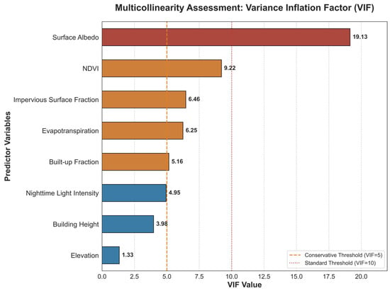
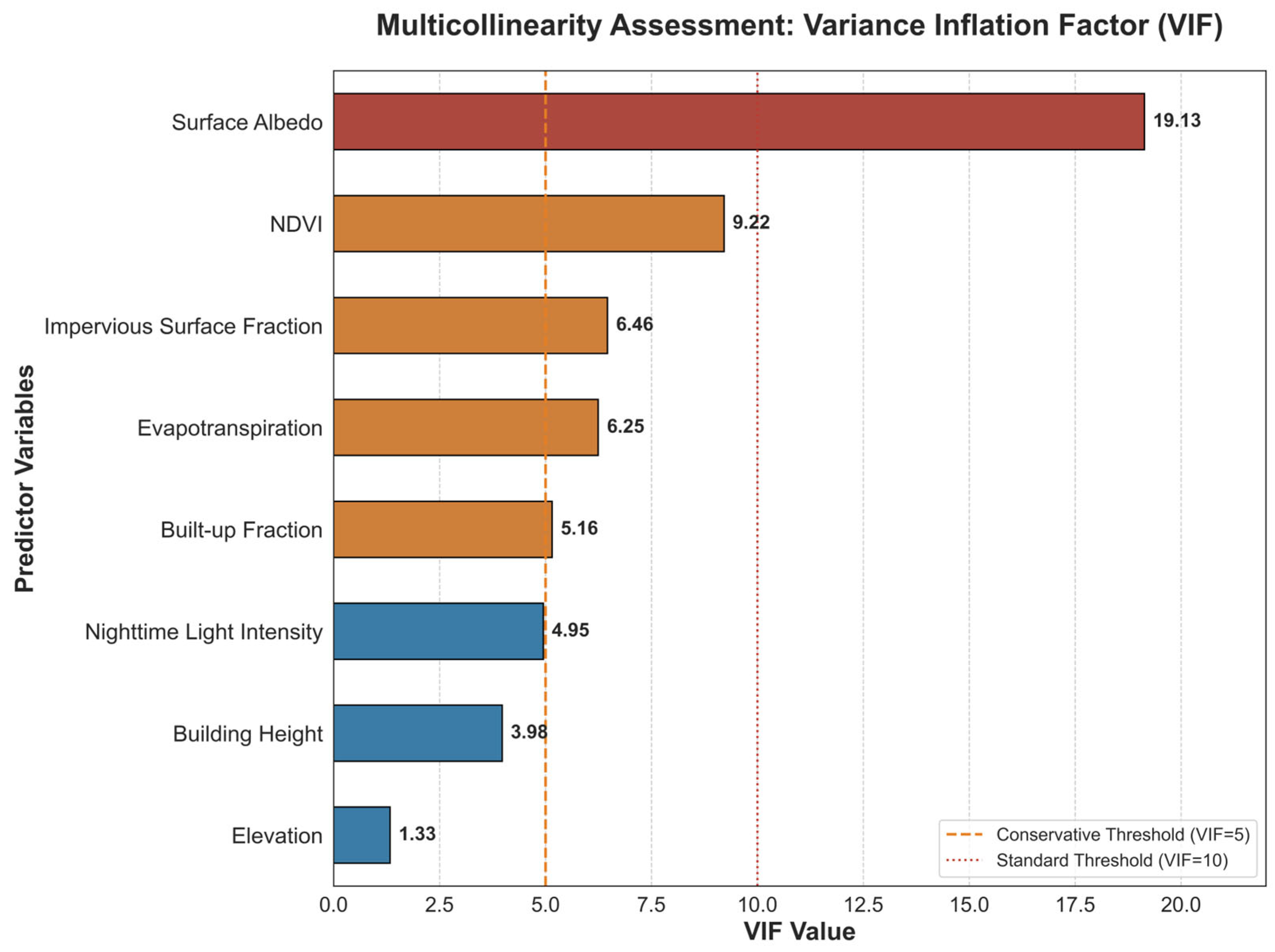
To evaluate potential multicollinearity among variables, a VIF analysis was conducted prior to the statistical analysis (Figure 1). Most variables exhibited low to moderate multicollinearity, with VIF values generally below or near commonly used thresholds (VIF = 5–10). Surface albedo showed the highest VIF value (19.13), indicating stronger covariance with other vegetation- and surface-related variables, whereas NDVI, evapotranspiration, impervious surface fraction, built-up fraction, and nighttime light intensity exhibited moderate covariance reflecting the coupled nature of urban environmental and morphological processes. Although the built-up and impervious surface fractions were only partially correlated, both variables were retained because they represent different dimensions of urban structure: the built-up fraction describes constructed surface density, and the impervious surface fraction reflects broader land-cover sealing conditions. Since the objective of this study was to investigate relationships among urban thermal, vegetation, and structural factors rather than to optimize predictive features, the VIF analysis was primarily used as a diagnostic assessment of variable dependence and interpretability, rather than as a strict criterion for variable exclusion.
Figure 1.
Multicollinearity Assessment of Urban Surface Predictors Using the Variance Inflation Factor (VIF).
2.3. Methodology
To systematically analyze the moderating effect of urban structure on vegetation CE, this study adopts a three-step analysis framework: (1) estimating the vegetation CE of each city based on the intra-city regression model to characterize its cross-city differences; (2) introducing the proportion of built-up fraction as a structural variable and analyzing the variation characteristics of CE under different urban structure conditions through hierarchical regression analysis; (3) constructing a machine learning model based on XGBoost and interpreting the influence of each variable by combining the SHAP method. To ensure interpretative reliability, this framework further incorporates a dual-validation approach: using city-specific regressions to confirm the statistical significance of identified trends and residual analysis to verify the predictive stability across diverse urban contexts.
So, this framework integrates functional estimation, structural moderation, and flexible modeling to provide a comprehensive assessment of vegetation-induced thermal regulation [38].
2.3.1. Estimation of Cross-City Vegetation CE
To quantify the thermal regulation capacity of urban vegetation, we estimated vegetation CE at the city scale using a within-city regression framework. The CE index was defined as the absolute slope of the linear relationship between and NDVI within each city-year group, representing the relative cooling sensitivity associated with vegetation variation. For each city and year, pixel-level observations were used to fit a linear regression model between NDVI and . The resulting regression slope quantified the magnitude of the vegetation-associated cooling response under different urban and climatic conditions.
Because macro-climatic forcing (e.g., regional temperature regime, solar radiation, large-scale atmospheric circulation) is relatively homogeneous within an individual city boundary, spatial variability in LST across pixels is primarily driven by land surface properties, including vegetation cover and built-up fraction [18,20,28]. This within-city design therefore isolates the intrinsic thermal sensitivity to vegetation while minimizing confounding from inter-city climatic differences [28].
For each city-year group, the following linear model was estimated:
where represents the normalized LST at pixel in city during year , and denotes the corresponding NDVI. The intercept represents the baseline thermal condition, while the slope coefficient quantifies the thermal response associated with vegetation variation.
The CE index was defined as:
Larger values indicate stronger vegetation-associated cooling sensitivity. OLS regression was applied separately to each city-year group.
To ensure statistical robustness, pixels with missing NDVI or LST values were removed prior to estimation. In addition, slope estimation was performed only when a city contained at least 30 valid observations, reducing instability from small-sample regression bias. Importantly, this framework measures thermal sensitivity rather than absolute cooling magnitude [23]. A city with high overall vegetation coverage may still exhibit weak CE if temperature is not strongly responsive to NDVI variation. Conversely, a city with limited vegetation can display strong CE if marginal increases in NDVI produce substantial temperature reductions. This distinction allows the analysis to focus on functional thermal regulation strength rather than vegetation abundance alone.
2.3.2. Estimation of CE Constrained by Built-Up Fraction
Urban thermal dynamics are shaped not only by vegetation abundance but also by the built environment’s structural configuration [20,24]. Urban morphology influences airflow, radiation trapping, heat storage capacity, and surface energy balance, all of which may alter how effectively vegetation mitigates surface temperature [39,40]. In highly compact urban fabrics, increased impervious coverage, anthropogenic heat release, and reduced ventilation may weaken the marginal cooling benefit provided by vegetation patches [41]. Against this structural backdrop, the relationship between NDVI and LST may vary across different levels of urban compaction. While the baseline city-level estimation captures overall cooling sensitivity, it does not explicitly distinguish whether the vegetation-temperature coupling changes systematically along built-up fraction gradients [42,43].
To address this issue, built-up fraction was incorporated as a stratification variable within the NDVI–LST analysis framework. Built-up fraction values derived from the GHSL built-up surface dataset were standardized to fractional values ranging from 0 to 1 and subsequently categorized into five intervals (0%–20%, 20%–40%, 40%–60%, 60%–80%, and 80%–100%), representing progressively intensified urban development conditions from low-density suburban areas to highly compact urban cores. The relationship between NDVI and LST norm was then examined separately within each built-up fraction interval and climate group using ordinary least squares regression visualization. This framework enabled comparison of vegetation-associated thermal response patterns across different urban structural intensities while avoiding assumptions of a globally uniform NDVI–LST relationship.
Cooling attenuation was evaluated by comparing the magnitude of NDVI–LST regression slopes across different built-up fraction categories. Steeper negative slopes indicate stronger thermal sensitivity of LST to vegetation variation, whereas flatter slopes reflect weaker vegetation-associated cooling responses. This stratified framework enables the influence of urban structural intensity on vegetation CE to be examined under comparable climatic conditions. Rather than quantifying vegetation abundance alone, the analysis focuses on how urban morphology modifies the functional relationship between vegetation greenness and LST.
2.3.3. Interpretable Machine Learning as Complementary Analysis
To further examine the generality of the context-dependent cooling patterns identified above, we implemented a machine learning regression framework as a complementary analysis. While the preceding sections quantified vegetation CE and its built-up fraction variation through explicit regression specifications, this step allows nonlinear responses and complex interactions to emerge flexibly from the data. Pixel-level LST was modeled as a function of NDVI, surface albedo, elevation, nighttime light intensity, built-up fraction, impervious surface fraction, and evapotranspiration using XGBoost. XGBoost is an ensemble learning method based on sequentially constructed decision trees, where each tree incrementally improves prediction accuracy by minimizing a differentiable loss function [32,44]. Its boosting structure enables the model to capture nonlinear relationships and higher-order interactions without requiring prior specification of functional form [32]. Model performance was evaluated using out-of-sample prediction metrics ( and RMSE) [33,44].
To interpret the contribution of predictors, SHAP values were computed to quantify each variable’s marginal influence on LST predictions [45,46]. The SHAP provides a consistent attribution framework grounded in cooperative game theory, enabling decomposition of model output into additive feature contributions [47,48]. This complementary analysis enables assessment of whether the modulation of vegetation cooling by built-up fraction and surface properties remains evident under a flexible, non-parametric formulation [49,50].
3. Results
3.1. Vegetation CE Varies Across Cities
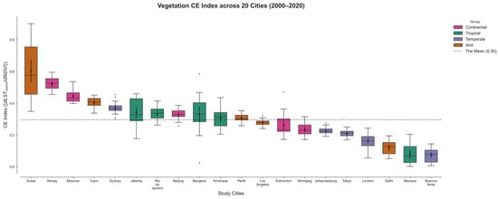
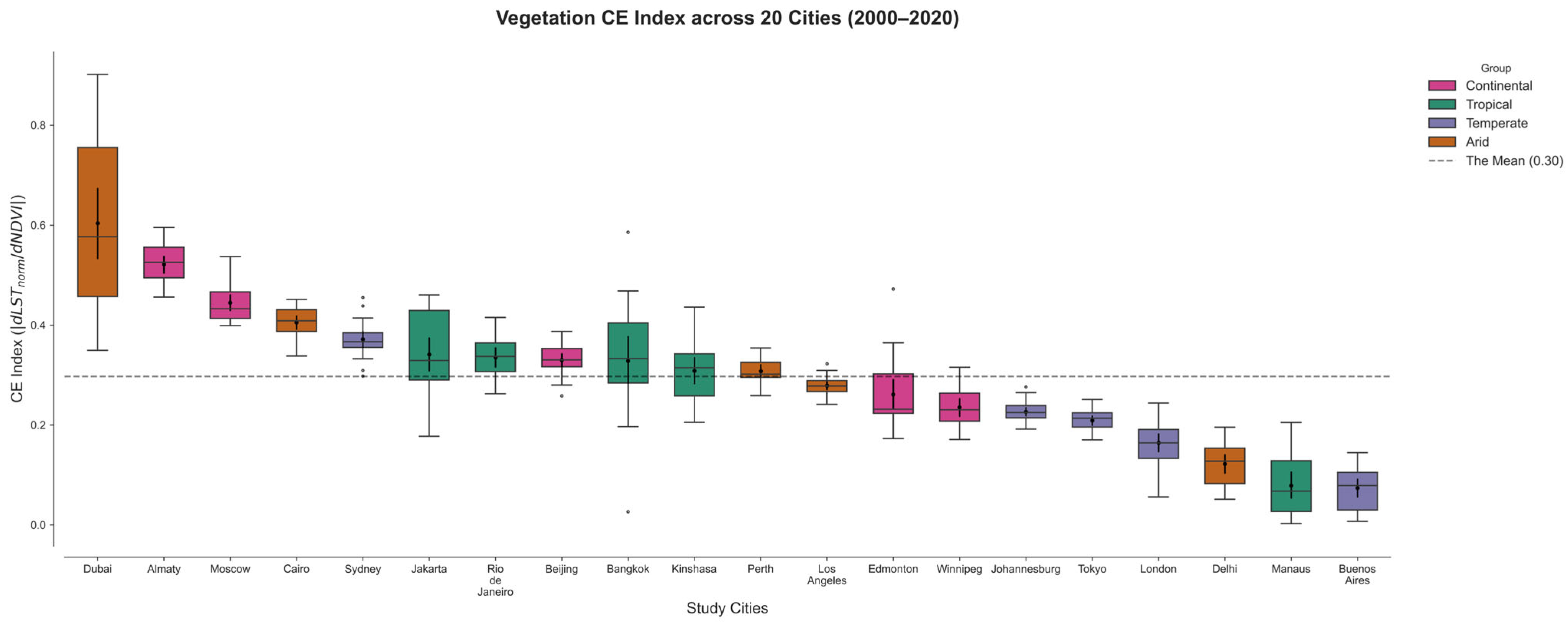
There is a substantial heterogeneity in vegetation CE across the selected 20 major cities worldwide (Figure 2). The vegetation CE showed substantial inter-city variability, with a mean value of approximately 0.3, ranging from 0.07 to 0.60. Cities can generally be categorized into the following three groups based on their CE.
Figure 2.
Distribution of Vegetation CE Across 20 Cities Worldwide (2000–2020). CE was estimated separately for each city-year group as the slope of the NDVI–LST relationship. Boxplots summarize the distribution of annual CE values over the study period.
- High CE Cities
Cities with CE values substantially above the global mean included Dubai (0.60), Almaty (0.52), Moscow (0.45), Cairo (0.41), and Sydney (0.37). Among these, Dubai showed the strongest vegetation cooling performance, with CE values ranging from 0.35 to 0.90, indicating exceptionally high thermal sensitivity to vegetation presence in arid environments. Similarly, continental cities such as Almaty and Moscow exhibited relatively high CE values.
- Intermediate CE Cities
CE values in several cities clustered around the global average, including Jakarta (0.34), Rio de Janeiro (0.34), Beijing (0.33), Bangkok (0.33), Kinshasa (0.31), and Perth (0.31). These cities generally showed moderate vegetation CE with comparatively broader variability distributions, particularly in tropical cities such as Bangkok and Jakarta.
- Low CE Cities
Cities with CE values below the mean included Los Angeles (0.28), Edmonton (0.26), Winnipeg (0.24), Johannesburg (0.23), Tokyo (0.21), London (0.16), Delhi (0.12), Manaus (0.08), and Buenos Aires (0.07). The weakest vegetation cooling performance was observed in Buenos Aires. In several highly urbanized temperate cities, including London and Tokyo, vegetation CE remained consistently low.
Importantly, these results demonstrate that: a high vegetation presence does not guarantee a high CE. Cooling sensitivity must be evaluated functionally rather than descriptively. LST regulation operates under differentiated regimes across global cities.
3.2. Vegetation CE Constrained by Built-Up Fraction
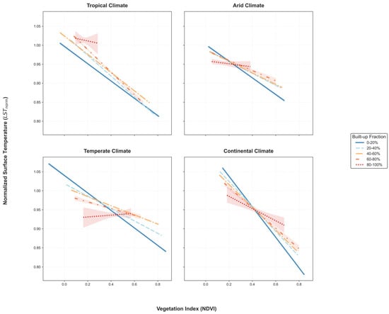
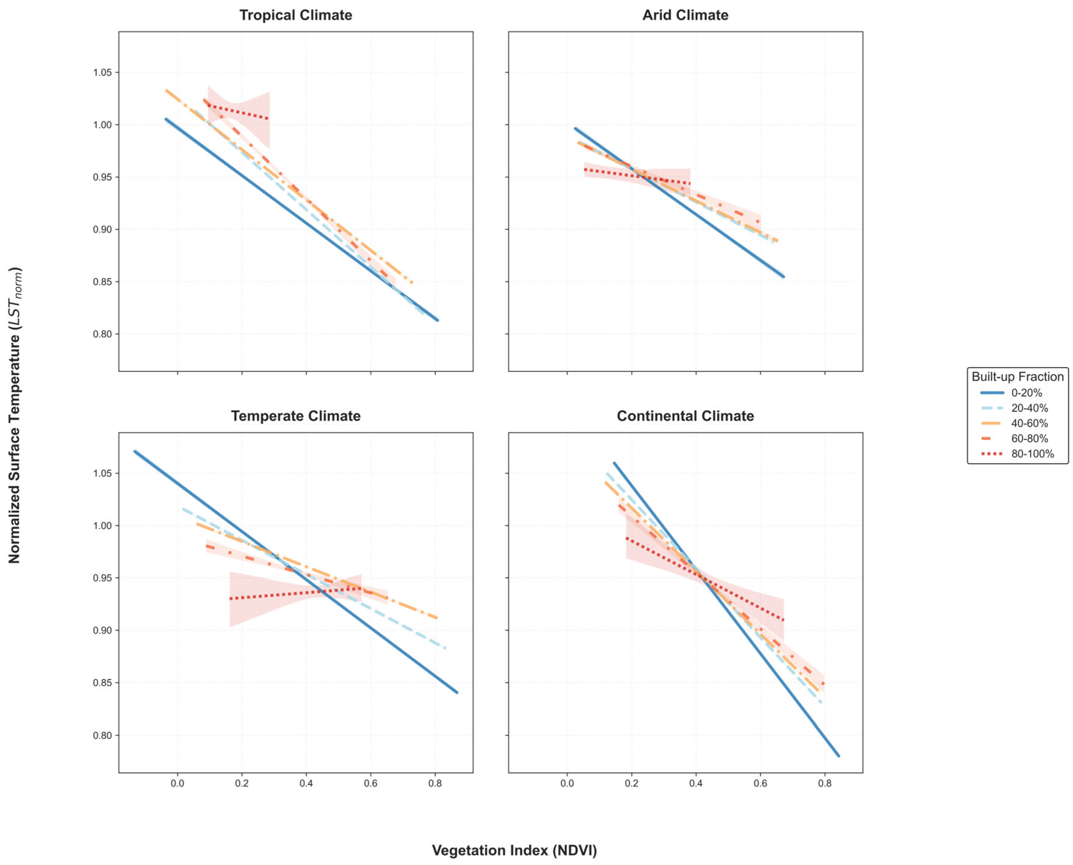
To evaluate the cooling constraint imposed by built-up fraction, vegetation CE was estimated separately across built-up fraction gradients. The relationship between NDVI and LST varied substantially across climatic backgrounds and built-up fraction categories (Figure 3). Overall, higher NDVI values were consistently associated with lower LST, although the magnitude of the cooling response varied markedly across climate zones and levels of urban density.
Figure 3.
Climate-Dependent Relationships Between NDVI and LST Across Built-up Fraction Gradients. Total sample sizes were n = 82,451 for tropical cities, n = 75,747 for arid cities, n = 97,167 for continental cities, and n = 136,437 for temperate cities.
In tropical cities, all built-up fraction categories exhibited negative NDVI–LST relationships. Cooling slopes remained broadly comparable across most urban density classes, while a noticeable reduction in cooling sensitivity was observed only in the highest built-up category (80%–100%).
Arid cities showed relatively similar NDVI–LST relationships across all built-up fraction categories. Although vegetation cooling performance remained evident throughout the urban density gradient, differences among built-up categories were comparatively small, resulting in nearly parallel regression trends. The overall cooling gradients across the NDVI range were also relatively short compared with those observed in tropical and continental cities.
Temperate cities were the most sensitive to increasing built-up fraction. Strong negative NDVI–LST relationships were observed in low-density built-up fraction, while cooling slopes declined markedly as built-up fraction increased. In the highest built-up category (80%–100%), a weak positive NDVI–LST relationship emerged.
Continental cities maintained strong vegetation cooling responses across most built-up categories. Negative NDVI–LST relationships remained evident in both low- and medium-density urban environments, although some attenuation was observed in the highest built-up class. Overall, continental cities displayed the steepest cooling gradients among the four climate groups.
Across all climate groups, a consistent pattern emerged: an increasing built-up fraction weakened the NDVI–LST relationship. The 0%–20% built-up category generally exhibited the strongest cooling response, whereas the 80%–100% category consistently showed the weakest response. This attenuation pattern was observed across all four climate groups, although its magnitude varied among climatic contexts.
3.3. Machine Learning Validation of Structural Constraint
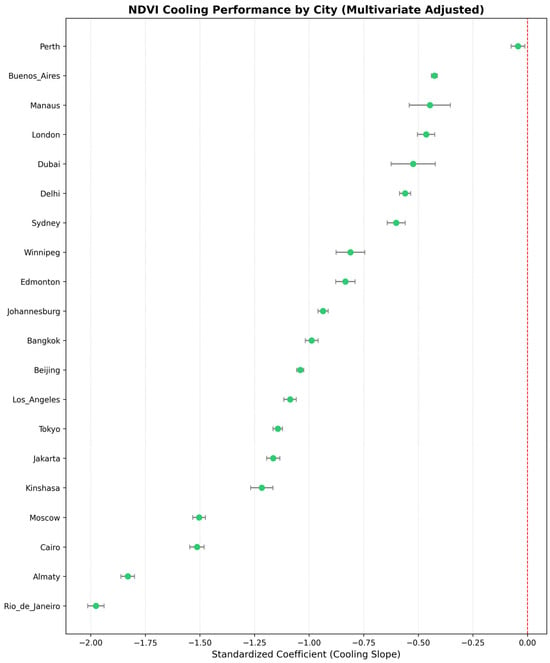
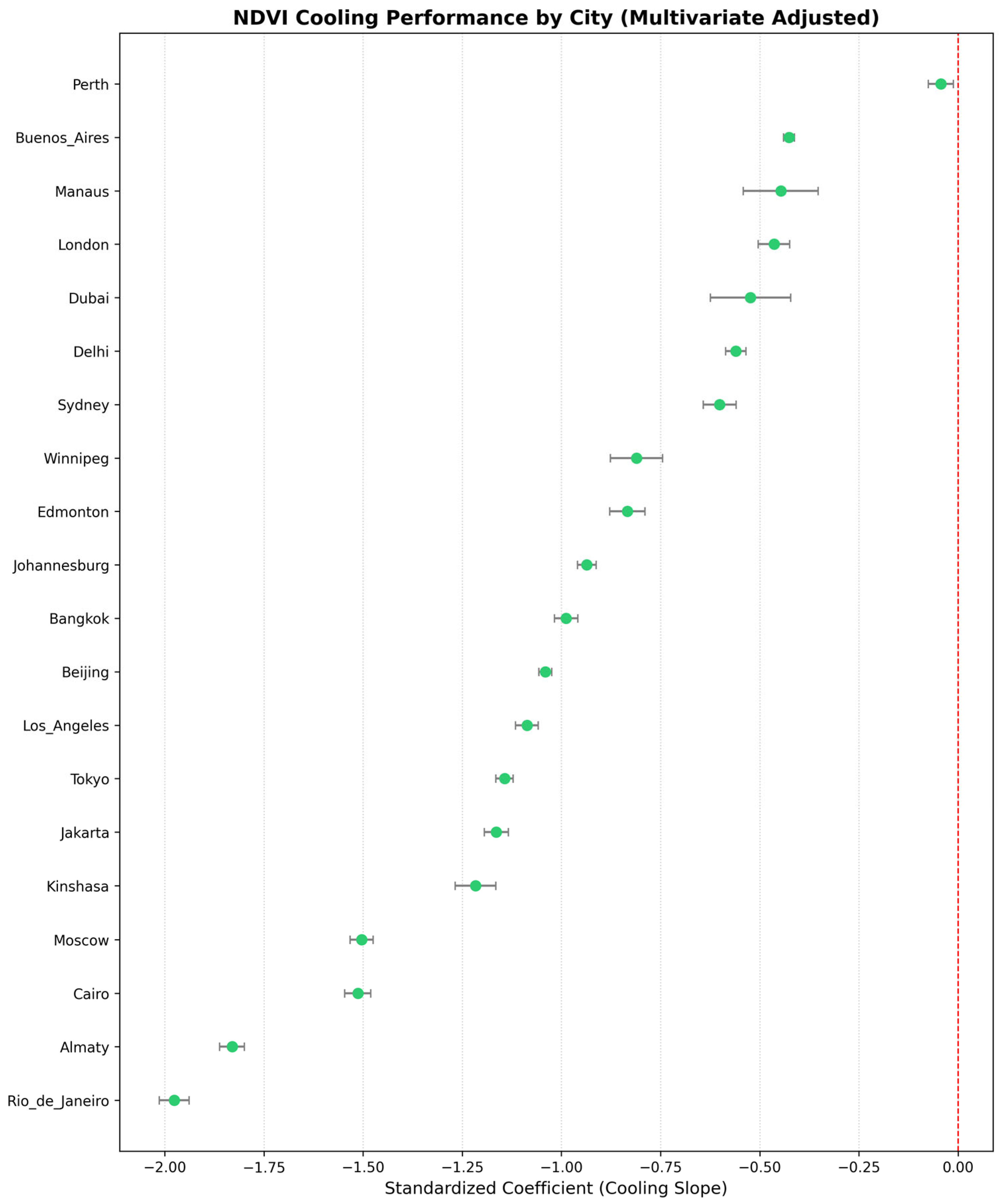
To further evaluate the robustness of vegetation cooling performance across heterogeneous urban environments, firstly, city-specific multivariate regression models were developed by incorporating additional environmental and urban predictors, including surface albedo, elevation, impervious surface fraction, built-up fraction, building height, and evapotranspiration (Figure 4). After controlling for the selected covariates, all cities retained negative standardized NDVI coefficients (β), indicating persistent vegetation-associated cooling performance across diverse urban contexts. Standardized NDVI coefficients ranged from approximately −1.98 to −0.05. Rio de Janeiro, Almaty, Cairo, and Moscow exhibited the strongest vegetation cooling performance, whereas Perth, Buenos Aires, Manaus, and London showed the weakest. Most cities showed relatively narrow confidence intervals around the estimated coefficients.
Figure 4.
City-specific cooling performance of vegetation after multivariate adjustment. Points represent standardized NDVI regression coefficients (β) derived from multivariate regression models after controlling for albedo, elevation, impervious surface fraction, built-up fraction, built height, and evapotranspiration. Horizontal error bars indicate 95% confidence intervals.
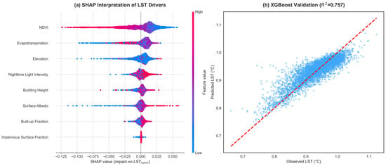
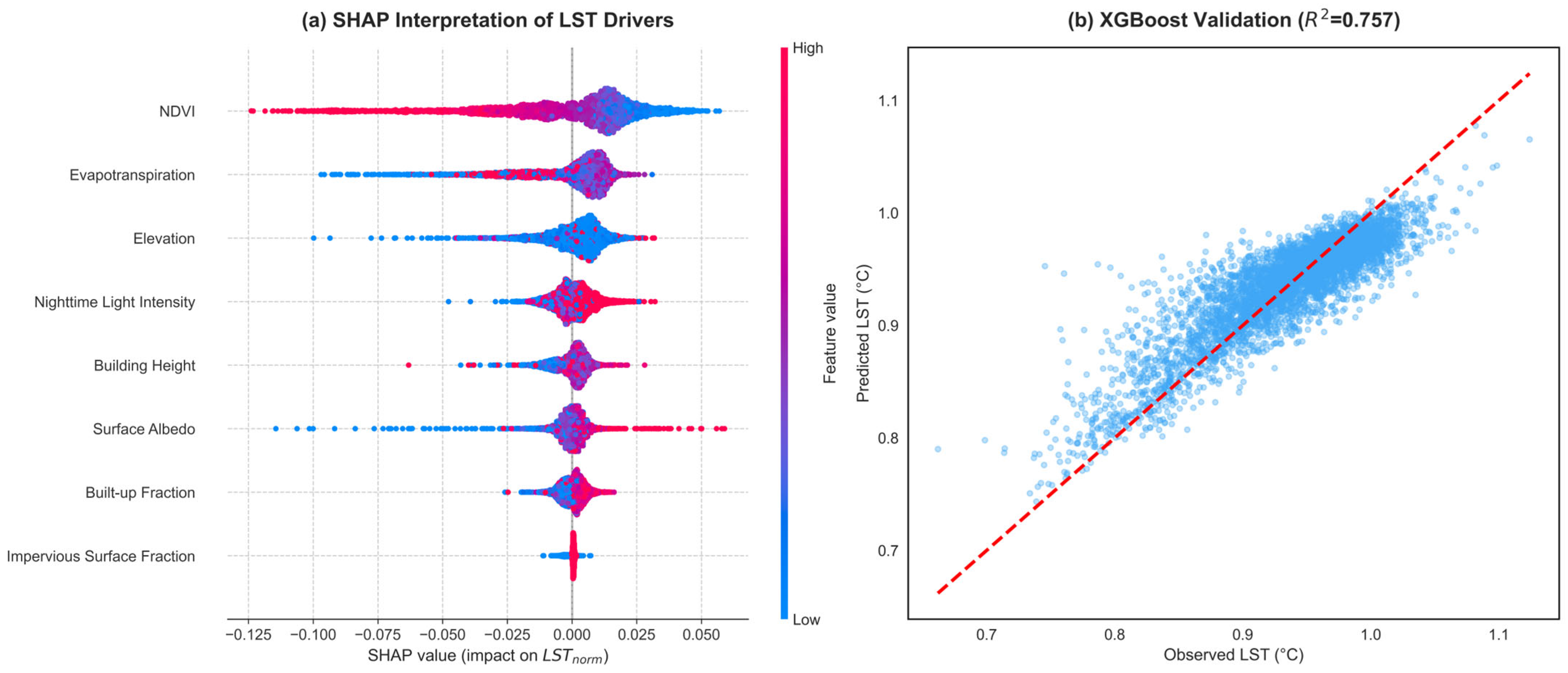
Figure 5a presents the SHAP-based contributions of environmental and urban variables to LST prediction. NDVI had the highest overall contribution magnitude (mean |SHAP| = 0.021), followed by evapotranspiration (mean |SHAP| = 0.012). Elevation showed moderate contributions (mean |SHAP| = 0.007), whereas urban structural variables, including nighttime light intensity, building height, built-up fraction, and impervious surface fraction, generally contributed less to LST prediction. Overall, vegetation-related variables displayed broader SHAP distributions than urban morphological indicators. Figure 5b shows the predictive performance of the XGBoost model, which achieved an out-of-sample R2 of 0.757. Predicted values closely aligned with observed LST across the full temperature range.
Figure 5.
SHAP-based interpretation and XGBoost validation of LST drivers. (a) SHAP summary plot showing the distribution, direction, and relative magnitude of variable contributions to LST predictions. Each point represents an individual pixel-level observation, with colors indicating relative feature values from low to high. (b) Comparison between observed and XGBoost-predicted LST values, with the dashed red line representing the 1:1 relationship between observations and model predictions.
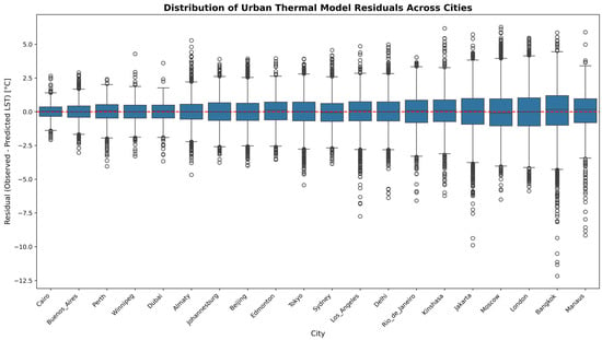
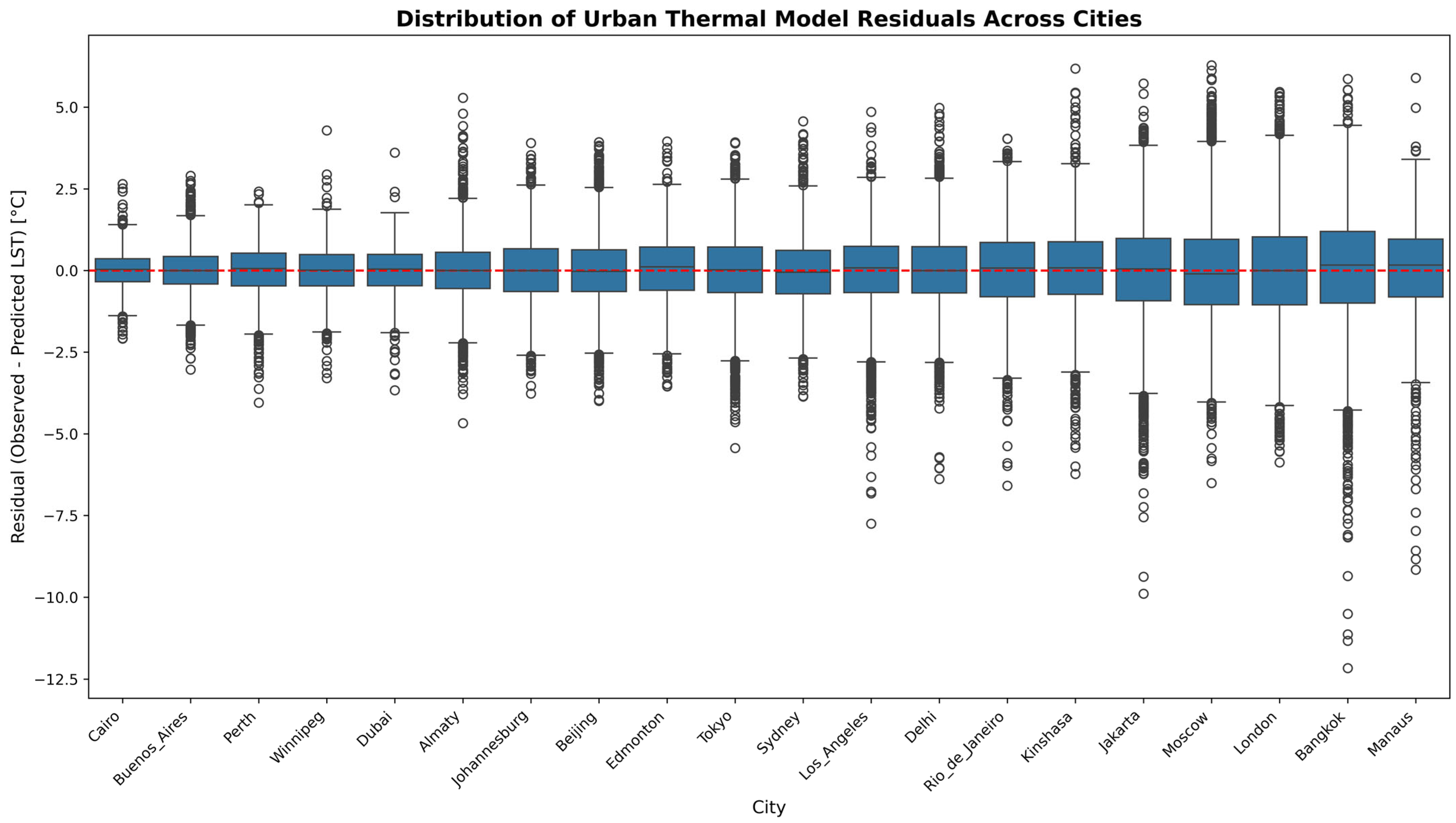
Furthermore, residual distributions were examined to evaluate cross-city variability in model performance (Figure 6). Residual medians remained close to zero across all cities, indicating limited systematic prediction bias. Cairo (RMSE = 0.54 °C), Buenos Aires (0.66 °C), Perth (0.77 °C), and Winnipeg (0.81 °C) showed relatively compact residual distributions with smaller interquartile ranges (IQRs), whereas Jakarta (1.54 °C), Moscow (1.58 °C), London (1.59 °C), Bangkok (1.74 °C), and Manaus (1.78 °C) exhibited broader residual spreads and larger IQRs. Despite these differences, most residuals remained within approximately ±2 °C of the zero-reference line, supporting the overall robustness of the modeling framework across diverse urban environments.
Figure 6.
Distribution of Urban Thermal Model Residuals Across Global Cities. Residuals were calculated as the difference between observed and XGBoost-predicted LST values. Boxplots summarize the median, interquartile range (IQR), and residual dispersion for each city. Whiskers extend to 1.5 × IQR, while circles represent outliers beyond this range. The horizontal dashed red line indicates zero-residual reference, where predicted and observed LST values are equal.
4. Discussion
4.1. Context-Dependent Variability in Vegetation CE
By integrating city-level regression, analysis constrained by built-up fraction, and complementary machine learning modeling, the results demonstrate substantial cross-city variation in vegetation CE and show that the NDVI–LST relationship varies systematically across built-up fraction gradients across different climatic contexts. Vegetation cooling should not be regarded as a fixed or universally consistent ecological function, but rather as a climate-dependent response shaped by background environmental conditions. This interpretation is consistent with the findings of Li et al. [51] and Wang et al. [52], who also showed that the cooling performance of urban vegetation is strongly climate-dependent.
Arid and semi-arid region cities displayed the strongest inter-city divergence in CE. The exceptionally high CE observed in Dubai suggests that irrigated vegetation may still maintain strong thermal contrasts within highly compact desert environments, whereas the weaker cooling response observed in Delhi implies that persistent heat stress and moisture limitations may constrain vegetation-related thermal regulation. This finding is consistent with previous studies describing oasis-like cooling performances in irrigated arid cities and reduced vegetation cooling performance under extreme urban heat stress conditions [53,54].
Temperate-region cities such as London and Tokyo showed progressively weaker NDVI–LST cooling gradients as the built-up fraction increased, reflecting reduced vegetation cooling performance under highly compact urban conditions. Previous studies have similarly reported that dense urban morphology, enhanced surface heat storage, and reduced ventilation efficiency can weaken the marginal cooling sensitivity associated with fragmented urban vegetation [55,56,57]. Notably, under extremely high built-up conditions (80%–100%), several temperate urban cores showed near-neutral or even slightly positive NDVI–LST relationships, implying that vegetation-associated cooling performance may become substantially diminished or locally ineffective once urban compactness exceeds certain thresholds.
In contrast, several tropical-region cities, including Jakarta and Rio de Janeiro, retained detectable vegetation cooling across all built-up categories, although cooling gradients also weakened under highly urbanized conditions. Buyantuyev and Wu showed that landscape heterogeneity within urban environments can strongly influence localized thermal patterns, particularly where impervious surfaces and fragmented vegetation patches are closely interwoven [58]. Mokhtari et al. further suggested that spatial heterogeneity in compact urban environments may enhance localized thermal contrasts and contribute to uneven urban heat responses [59]. Under persistently warm and humid climatic conditions, vegetation-associated cooling responses in tropical cities remained observable across the urban density gradient, although the magnitude of cooling declined with increasing urban compactness.
Continental-region cities presented relatively strong cooling sensitivity under lower built-up conditions, although these cooling gradients weakened progressively with increasing urbanization intensity. Compared with tropical cities, the cooling responses observed in continental systems appeared more sensitive to increases in the built-up fraction, indicating a stronger reduction in vegetation cooling performance with increasing urban compactness.
Despite substantial inter-city variability within climate groups, cooling responses to increasing urbanization followed distinct patterns across climatic contexts. Tropical cities generally retained detectable cooling sensitivity across all urban density classes, although cooling performance weakened as built-up fraction increased, whereas temperate cities showed progressive cooling attenuation and, under extreme urban density, locally shifted toward neutral or slightly positive NDVI–LST relationships. Arid cities showed the greatest variability, with cooling responses differing substantially among them despite broadly similar water-limited climatic conditions. These patterns indicate that the thermal response of urban vegetation is not random across cities but systematically mediated by climatic background and urban form. Our results highlight the importance of considering background climatic conditions when evaluating the thermal benefits of urban vegetation, while the implications of these climate-specific cooling responses for urban heat mitigation and planning are discussed further [21,60].
4.2. Interpretable Machine Learning as Mechanistic Validation
A key methodological contribution of this study is the integration of an interpretable machine learning framework with the regression-based CE framework. Traditional urban climate studies have long relied on OLS regression or conventional panel-based statistical models to examine relationships between LST and environmental drivers. While these approaches provide relatively strong parameter interpretability, they generally assume globally fixed linear relationships and therefore may struggle to fully capture the nonlinear interactions, spatial heterogeneity, and contextual dependency commonly observed in complex urban systems [61]. In contrast, the interpretable machine learning framework based on XGBoost and SHAP introduced in this study not only demonstrated strong predictive robustness (out-of-sample R2 = 0.757) but also provided a more flexible analytical perspective for understanding the complexity of vegetation cooling relationships across different climate–urban contexts.
First, the interpretable machine learning framework enables nonlinear thermal interactions to emerge directly from the data without requiring predefined functional forms. Urban thermal processes are inherently governed by coupled interactions among vegetation, evapotranspiration, surface albedo, built-up fraction, and anthropogenic activities, many of which exhibit substantial covariance [18,62]. Multicollinearity diagnostics revealed moderate to strong covariance among several variables, with albedo recording the highest VIF value (19.13). Under conventional regression frameworks, such covariance structures may complicate parameter interpretation or reduce model stability. By contrast, the ensemble tree-based structure of XGBoost allows complex thermal response relationships to be captured while preserving the full multivariate environmental context. Further SHAP analysis showed that NDVI and evapotranspiration consistently maintained strong contributions to thermal regulation across different urban environments, whereas several urban morphological variables exhibited more pronounced nonlinear and spatially heterogeneous response patterns.
In addition, interpretable machine learning proved useful for examining spatial heterogeneity and potential non-stationarity in global urban thermal systems. As discussed in Section 4.1, vegetation cooling responses varied substantially across climatic and urban structural contexts, indicating that urban thermal regulation may not follow a globally uniform response structure. Li et al. suggested that conventional statistical frameworks based on globally fixed relationships lack the flexibility to capture context-dependent thermal dynamics under such heterogeneous urban conditions [23]. Residual analysis further revealed systematic differences in model stability across cities, with several tropical cities exhibiting broader residual distributions and greater prediction variability, suggesting more complex localized thermal interactions in these urban environments. Despite this spatial heterogeneity, residual medians across most cities remained centered near the zero-reference line, indicating relatively robust cross-regional model performance overall. Compared with relying on a single globally fixed statistical relationship to characterize urban thermal systems, interpretable non-parametric machine learning frameworks may therefore provide a more flexible approach for examining highly heterogeneous urban environments [30].
From a broader methodological perspective, this study also highlights the potential of GeoAI (Geospatial Artificial Intelligence) approaches for global urban climate research. As global-scale remote sensing datasets, multi-source urban datasets, and high-dimensional environmental variables continue to expand rapidly, traditional statistical frameworks face increasing challenges in representing complex interactions and regional heterogeneity [30]. In contrast, interpretable machine learning approaches can improve the representation of nonlinear environmental relationships while preserving the complexity of urban systems [31]. Particularly in cross-regional and multi-climate comparative studies, such frameworks allow global urban thermal relationships to be examined while still retaining local contextual variability [45]. In this sense, GeoAI should not be viewed as a replacement for conventional statistical approaches, but rather as a complementary analytical framework that supports the identification of nonlinear relationships and the interpretation of heterogeneous patterns within complex geographic systems.
Overall, regression-based analysis in this study provides explicit quantitative estimates of CE, while interpretable machine learning further reveals the persistence, nonlinear characteristics, and spatial heterogeneity of vegetation cooling relationships under complex urban conditions. These approaches provide an integrated analytical pathway for future global urban thermal research that balances mechanistic interpretability, complex system representation, and cross-regional comparative capability.
4.3. Implications for Urban Heat Mitigation
The observed differences in vegetation cooling responses across climatic backgrounds and built-up intensities demonstrate that the thermal benefits of urban greening are not globally uniform [63,64]. Similar increases in vegetation may correspond to substantially different cooling responses under different climate–urban configurations [65]. Across built-up fraction gradients, vegetation CE, response magnitude, and response stability all varied considerably, indicating that vegetation cooling in urban environments is better understood as a context-dependent thermal regulation process rather than a simple linear outcome determined solely by vegetation quantity.
These findings carry important implications for urban heat mitigation strategies. Existing urban greening policies often emphasize vegetation quantity indicators, such as canopy coverage or total greening area, while implicitly assuming that greater vegetation coverage will necessarily produce stronger cooling benefits [66,67]. However, vegetation quantity alone may not be a reliable indicator of thermal regulation performance. Even under similar vegetation coverage levels, cooling responses differed substantially among cities and climate systems. In this context, functional metrics such as CE may provide a more informative measure of vegetation cooling performance by directly quantifying the thermal benefits generated under specific urban structural and climatic conditions. Future urban heat mitigation studies may benefit from shifting from a vegetation quantity-oriented perspective toward a cooling performance-oriented framework.
The results also show that urban greening strategies may require more climate-sensitive planning approaches rather than relying on uniform greening models. The observed differences among climate groups indicate that vegetation cooling effectiveness is influenced not only by vegetation abundance but also by broader climatic and urban conditions. In tropical cities, vegetation cooling performance remained relatively persistent across most urban settings, whereas temperate cities appeared more sensitive to increasing urban compactness, leading to reduced cooling performance. Cooling responses varied considerably among arid cities, highlighting the importance of local moisture conditions and urban management in shaping vegetation-mediated cooling. Therefore, similar greening interventions may yield different thermal outcomes across cities, underscoring the importance of climate-specific urban heat mitigation strategies.
In addition, the response variations observed across built-up fraction gradients suggest the presence of urbanization-related threshold behavior in vegetation CE. In several highly compact urban environments, increases in vegetation did not necessarily correspond to continuously enhanced cooling responses. This implies that, under extreme urban compactness, localized greening alone may not sustain the same level of thermal mitigation benefits observed in lower-density environments. Overall, the present study highlights the pronounced climate-dependent heterogeneity of vegetation cooling responses and suggests that future urban heat mitigation planning may benefit from more explicit consideration of climatic background, urban morphology, and vegetation cooling performance when developing climate-sensitive urban greening strategies.
4.4. Limitations and Future Directions
While this study provides consistent evidence across multiple analytical approaches, several limitations should be acknowledged. First, the analysis relies primarily on satellite-derived datasets harmonized to a common 1 km spatial resolution, which may not fully capture fine-scale intra-urban heterogeneity and lacks systematic ground-based validation. Second, although the study includes 20 cities across diverse climatic regions, the findings are based on a comparative case-based framework and may not be fully representative of all urban environments, particularly smaller or less densely developed cities. Third, the datasets originate from different sources and reference periods, which may introduce temporal inconsistencies and additional uncertainty in cross-city comparisons. Finally, although the machine learning framework achieved satisfactory predictive performance, additional factors such as detailed urban morphology, anthropogenic heat emissions, and spatially stratified validation could further improve model representation. Future research could address these limitations by using higher-resolution, temporally consistent datasets, expanding city coverage, and providing a more detailed characterization of urban structural conditions.
5. Conclusions
This study quantified vegetation CE across 20 major cities worldwide under varying climatic and urban structural conditions using a combined regression and interpretable machine learning framework. By integrating multi-source remote sensing datasets from 2000 to 2020, the study established a comparative framework for evaluating vegetation-associated cooling responses across climate groups and built-up fraction gradients. To improve inter-city comparability, normalized LST, LCZ-conditioned sampling, built-up fraction stratification, and harmonized warm-season composites were applied, enabling more consistent comparison across heterogeneous urban systems.
The results revealed substantial cross-city heterogeneity in vegetation CE. NDVI–LST relationships varied systematically across climatic and built-up conditions, suggesting that urban vegetation cooling is not a globally uniform ecological function, but rather a context-dependent thermal response shaped by climate background and urban morphology. An increase in the built-up fraction was generally associated with weaker or more unstable cooling responses, although the magnitude and stability of this attenuation varied across climate zones. The results have important implications for urban heat mitigation and planning, indicating that vegetation-based cooling strategies should not rely on generalized greening assumptions but rather require climate-sensitive, morphology-aware planning approaches adapted to local urban conditions.
The interpretable machine learning analysis further demonstrated the value of nonlinear analytical frameworks for examining complex urban thermal systems. XGBoost and SHAP analyses showed that vegetation-related variables consistently contributed strongly to LST variability, whereas several urban morphological variables exhibited more heterogeneous response patterns across cities. The study highlights the growing potential of GeoAI approaches for investigating nonlinear, heterogeneous, and context-dependent urban climate processes at the global scale. By integrating regression-based CE quantification with interpretable machine learning analysis, this study provides a complementary methodological framework for future comparative urban climate research and advances understanding of how vegetation cooling emerges from climate–urban interactions rather than from universally fixed thermal relationships.
Supplementary Materials
The following supporting information can be downloaded at: https://www.mdpi.com/article/10.3390/f17060707/s1.
Author Contributions
Conceptualization, L.H., H.N. and V.H.; methodology, L.H. and A.B.; software, L.H.; validation, L.H.; formal analysis, L.H.; investigation, L.H.; resources, L.H. and V.H.; data curation, L.H.; writing—original draft preparation, L.H.; writing—review and editing, L.H., H.N., A.B. and V.H.; visualization, L.H.; supervision, H.N. and V.H. All authors have read and agreed to the published version of the manuscript.
Funding
This research received no external funding.
Data Availability Statement
All datasets used in this study are publicly available through the Google Earth Engine (GEE) platform. The GEE script used for data extraction and preprocessing is publicly accessible at: https://code.earthengine.google.com/2444f1968ce55e25782a84365551921d (accessed on 14 June 2026).
Acknowledgments
During the preparation of this manuscript, the authors used ChatGPT (GPT-5.5, OpenAI, San Francisco, CA, USA) and Grammarly (Grammarly Inc., San Francisco, CA, USA) for grammar checking. All generated content was reviewed and edited by the authors, who take full responsibility for the final manuscript.
Conflicts of Interest
The authors declare no conflicts of interest.
References
- DePaul, M. Climate change, migration, and megacities: Addressing the dual stresses of mass urbanization and climate vulnerability. Paterson Rev. Int. Aff. 2012, 12, 145–162. [Google Scholar]
- Shen, P.; Zhao, S.; Ma, Y. Perturbation of Urbanization to Earth’s Surface Energy Balance. J. Geophys. Res. Atmos. 2021, 126, e2020JD033521. [Google Scholar] [CrossRef] [Scilit]
- Mohajerani, A.; Bakaric, J.; Jeffrey-Bailey, T. The urban heat island effect, its causes, and mitigation, with reference to the thermal properties of asphalt concrete. J. Environ. Manag. 2017, 197, 522–538. [Google Scholar] [CrossRef] [Scilit]
- Moore, M.; Gould, P.; Keary, B.S. Global urbanization and impact on health. Int. J. Hyg. Environ. Health 2003, 206, 269–278. [Google Scholar] [CrossRef] [Scilit]
- Johri, S.; Selvakumar, P.; Satyanarayana, P.; Das, A.; Gupta, S.; Bhattacharya, S. Urbanization and Energy: The Nexus of Global Challenges. In Geopolitical Landscapes of Renewable Energy and Urban Growth; IGI Global Scientific Publishing: Hershey, PA, USA, 2025; pp. 453–478. [Google Scholar]
- Tuholske, C.; Caylor, K.; Funk, C.; Verdin, A.; Sweeney, S.; Grace, K.; Peterson, P.; Evans, T. Global urban population exposure to extreme heat. Proc. Natl. Acad. Sci. USA 2021, 118, e2024792118. [Google Scholar] [CrossRef] [Scilit]
- Cleland, S.E.; Steinhardt, W.; Neas, L.M.; Jason West, J.; Rappold, A.G. Urban heat island impacts on heat-related cardiovascular morbidity: A time series analysis of older adults in US metropolitan areas. Environ. Int. 2023, 178, 108005. [Google Scholar] [CrossRef] [Scilit]
- Kumar, P.; Debele, S.E.; Khalili, S.; Halios, C.H.; Sahani, J.; Aghamohammadi, N.; Andrade, M.D.F.; Athanassiadou, M.; Bhui, K.; Calvillo, N.; et al. Urban heat mitigation by green and blue infrastructure: Drivers, effectiveness, and future needs. Innovation 2024, 5, 100588. [Google Scholar] [CrossRef] [Scilit] [PubMed]
- Hossain, M.L.; Li, J. NDVI-based vegetation dynamics and its resistance and resilience to different intensities of climatic events. Glob. Ecol. Conserv. 2021, 30, e01768. [Google Scholar] [CrossRef] [Scilit]
- Yue, W.; Xu, J.; Tan, W.; Xu, L. The relationship between land surface temperature and NDVI with remote sensing: Application to Shanghai Landsat 7 ETM+ data. Int. J. Remote Sens. 2007, 28, 3205–3226. [Google Scholar] [CrossRef] [Scilit]
- Garai, S.; Khatun, M.; Singh, R.; Sharma, J.; Pradhan, M.; Ranjan, A.; Rahaman, S.M.; Khan, M.L.; Tiwari, S. Assessing correlation between Rainfall, normalized difference Vegetation Index (NDVI) and land surface temperature (LST) in Eastern India. Saf. Extrem. Environ. 2022, 4, 119–127. [Google Scholar] [CrossRef] [Scilit]
- Mishra, B.; Sandifer, J.; Gyawali, B.R. Urban heat island in Kathmandu, Nepal: Evaluating relationship between NDVI and LST from 2000 to 2018. Int. J. Environ. 2019, 8, 17–29. [Google Scholar] [CrossRef] [Scilit]
- Rahimi, E.; Dong, P.; Jung, C. Global NDVI-LST Correlation: Temporal and Spatial Patterns from 2000 to 2024. Environments 2025, 12, 67. [Google Scholar] [CrossRef] [Scilit]
- Gao, M.; Piao, S.; Chen, A.; Yang, H.; Liu, Q.; Fu, Y.H.; Janssens, I.A. Divergent changes in the elevational gradient of vegetation activities over the last 30 years. Nat. Commun. 2019, 10, 2970. [Google Scholar] [CrossRef] [Scilit] [PubMed]
- Mukhtar, H.; Yang, Y.; Xu, M.; Wu, J.; Abbas, S.; Wei, D.; Zhao, W. Elevation-Dependent Vegetation Greening and Its Responses to Climate Changes in the South Slope of the Himalayas. Geophys. Res. Lett. 2025, 52, e2024GL113276. [Google Scholar] [CrossRef] [Scilit]
- Karnieli, A.; Agam, N.; Pinker, R.T.; Anderson, M.; Imhoff, M.L.; Gutman, G.G.; Panov, N.; Goldberg, A. Use of NDVI and Land Surface Temperature for Drought Assessment: Merits and Limitations. J. Clim. 2010, 23, 618–633. [Google Scholar] [CrossRef] [Scilit]
- Alavipanah, S.; Schreyer, J.; Haase, D.; Lakes, T.; Qureshi, S. The effect of multi-dimensional indicators on urban thermal conditions. J. Clean. Prod. 2018, 177, 115–123. [Google Scholar] [CrossRef] [Scilit]
- Oke, T.R.; Mills, G.; Christen, A.; Voogt, J.A. (Eds.) Concepts. In Urban Climates; Cambridge University Press: Cambridge, UK, 2017; pp. 14–43. [Google Scholar]
- Kuttler, W.; Weber, S. Characteristics and phenomena of the urban climate. Meteorol. Z. 2023, 32, 15–47. [Google Scholar] [CrossRef] [Scilit]
- Liang, Z.; Wu, S.; Wang, Y.; Wei, F.; Huang, J.; Shen, J.; Li, S. The relationship between urban form and heat island intensity along the urban development gradients. Sci. Total Environ. 2020, 708, 135011. [Google Scholar] [CrossRef] [Scilit]
- Moncada-Morales, G.A.; Verichev, K.; López-Guerrero, R.E.; Carpio, M. A Global Review of Vegetation’s Interaction Effect on Urban Heat Mitigation Across Different Climates. Urban Sci. 2025, 9, 361. [Google Scholar] [CrossRef] [Scilit]
- Aram, F.; Higueras García, E.; Solgi, E.; Mansournia, S. Urban green space cooling effect in cities. Heliyon 2019, 5, e01339. [Google Scholar] [CrossRef] [Scilit]
- Li, Y.; Svenning, J.-C.; Zhou, W.; Zhu, K.; Abrams, J.F.; Lenton, T.M.; Ripple, W.J.; Yu, Z.; Teng, S.N.; Dunn, R.R.; et al. Green spaces provide substantial but unequal urban cooling globally. Nat. Commun. 2024, 15, 7108. [Google Scholar] [CrossRef] [Scilit] [PubMed]
- Song, J.; Wang, Z.-H. Interfacing the Urban Land–Atmosphere System Through Coupled Urban Canopy and Atmospheric Models. Bound.-Layer Meteorol. 2015, 154, 427–448. [Google Scholar] [CrossRef] [Scilit]
- Sarker, I.H. Machine Learning: Algorithms, Real-World Applications and Research Directions. SN Comput. Sci. 2021, 2, 160. [Google Scholar] [CrossRef] [Scilit]
- Breiman, L. Random Forests. Mach. Learn. 2001, 45, 5–32. [Google Scholar] [CrossRef] [Scilit]
- Liakos, K.; Busato, P.; Moshou, D.; Pearson, S.; Bochtis, D. Machine Learning in Agriculture: A Review. Sensors 2018, 18, 2674. [Google Scholar] [CrossRef] [Scilit]
- Li, X.; Zhou, Y.; Asrar, G.R.; Imhoff, M.; Li, X. The surface urban heat island response to urban expansion: A panel analysis for the conterminous United States. Sci. Total Environ. 2017, 605–606, 426–435. [Google Scholar] [CrossRef] [Scilit] [PubMed]
- Ramesh, R. Modeling Urban Heat Island Intensity Using Satellite Imagery and Machine Learning; TechRxiv: Piscataway, NJ, USA, 2025. [Google Scholar] [CrossRef] [Scilit]
- Reichstein, M.; Camps-Valls, G.; Stevens, B.; Jung, M.; Denzler, J.; Carvalhais, N.; Prabhat. Deep learning and process understanding for data-driven Earth system science. Nature 2019, 566, 195–204. [Google Scholar] [CrossRef] [Scilit]
- Roscher, R.; Bohn, B.; Duarte, M.F.; Garcke, J. Explainable Machine Learning for Scientific Insights and Discoveries. IEEE Access 2020, 8, 42200–42216. [Google Scholar] [CrossRef] [Scilit]
- Friedman, J. Greedy Function Approximation: A Gradient Boosting Machine. Ann. Stat. 2001, 29, 1189–1232. [Google Scholar] [CrossRef] [Scilit]
- Hastie, T.; Tibshirani, R.; Friedman, J. The Elements of Statistical Learning; Springer Science & Business Media: New York, NY, USA, 2009. [Google Scholar] [CrossRef]
- Beck, H.E.; Zimmermann, N.E.; McVicar, T.R.; Vergopolan, N.; Berg, A.; Wood, E.F. Present and future Köppen-Geiger climate classification maps at 1-km resolution. Sci. Data 2018, 5, 180214. [Google Scholar] [CrossRef] [Scilit]
- Massaro, E.; Schifanella, R.; Piccardo, M.; Caporaso, L.; Taubenböck, H.; Cescatti, A.; Duveiller, G. Spatially-optimized urban greening for reduction of population exposure to land surface temperature extremes. Nat. Commun. 2023, 14, 2903. [Google Scholar] [CrossRef] [Scilit]
- Abdelkader, M.; Mendez, J.; Temimi, M.; Brown, D.; Spellman, K.; Arp, C.; Bondurant, A.; Kohl, H. A Google Earth Engine Platform to Integrate Multi-Satellite and Citizen Science Data for the Monitoring of River Ice Dynamics. Remote Sens. 2024, 16, 1368. [Google Scholar] [CrossRef] [Scilit]
- Demuzere, M.; Kittner, J.; Martilli, A.; Mills, G.; Moede, C.; Stewart, I.D.; Van Vliet, J.; Bechtel, B. A global map of local climate zones to support earth system modelling and urban-scale environmental science. Earth Syst. Sci. Data 2022, 14, 3835–3873. [Google Scholar] [CrossRef] [Scilit]
- Bowler, D.E.; Buyung-Ali, L.; Knight, T.M.; Pullin, A.S. Urban greening to cool towns and cities: A systematic review of the empirical evidence. Landsc. Urban Plan. 2010, 97, 147–155. [Google Scholar] [CrossRef] [Scilit]
- Jeon, G.; Park, Y.; Guldmann, J.-M. Impacts of Urban Morphology on Seasonal Land Surface Temperatures: Comparing Grid- and Block-Based Approaches. ISPRS Int. J. Geo-Inf. 2023, 12, 482. [Google Scholar] [CrossRef] [Scilit]
- Gomaa, M.M.; Nabil, J.; Berkouk, D.; Ragab, A. A Comparative Study of Vegetation Strategies for Outdoor Thermal Comfort in High- and Low-Density Urban Areas. Urban Sci. 2025, 9, 416. [Google Scholar] [CrossRef] [Scilit]
- Yin, S.; Liu, J.; Han, Z. Relationship between urban morphology and land surface temperature—A case study of Nanjing City. PLoS ONE 2022, 17, e0260205. [Google Scholar] [CrossRef] [Scilit] [PubMed]
- Cai, M.; Li, M.; Liu, H. Optimizing cooling efficiency of urban greenspaces across local climate zones in Wuhan, China. Urban For. Urban Green. 2025, 105, 128691. [Google Scholar] [CrossRef] [Scilit]
- Melaas, E.K.; Wang, J.A.; Miller, D.L.; Friedl, M.A. Interactions between urban vegetation and surface urban heat islands: A case study in the Boston metropolitan region. Environ. Res. Lett. 2016, 11, 054020. [Google Scholar] [CrossRef] [Scilit]
- Scott Lundberg, S.-I.L. A Unified Approach to Interpreting Model Predictions. arXiv 2017, arXiv:1705.07874. [Google Scholar] [CrossRef] [Scilit]
- Lundberg, S.M.; Erion, G.; Chen, H.; Degrave, A.; Prutkin, J.M.; Nair, B.; Katz, R.; Himmelfarb, J.; Bansal, N.; Lee, S.-I. From local explanations to global understanding with explainable AI for trees. Nat. Mach. Intell. 2020, 2, 56–67. [Google Scholar] [CrossRef] [Scilit]
- Feng, F.; Ren, Y.; Xu, C.; Jia, B.; Wu, S.; Lafortezza, R. Exploring the non-linear impacts of urban features on land surface temperature using explainable artificial intelligence. Urban Clim. 2024, 56, 102045. [Google Scholar] [CrossRef] [Scilit]
- Štrumbelj, E.; Kononenko, I. Explaining prediction models and individual predictions with feature contributions. Knowl. Inf. Syst. 2014, 41, 647–665. [Google Scholar] [CrossRef] [Scilit]
- Gramegna, A.; Giudici, P. SHAP and LIME: An Evaluation of Discriminative Power in Credit Risk. Front. Artif. Intell. 2021, 4, 752558. [Google Scholar] [CrossRef] [Scilit] [PubMed]
- Hoffman, J.S.; Shandas, V.; Pendleton, N. The Effects of Historical Housing Policies on Resident Exposure to Intra-Urban Heat: A Study of 108 US Urban Areas. Climate 2020, 8, 12. [Google Scholar] [CrossRef] [Scilit]
- Shafizadeh-Moghadam, H.; Liu, H.; Valavi, R. Modeling the spatial variation of urban land surface temperature in relation to environmental and anthropogenic factors: A case study of Tehran, Iran. GIScience Remote Sens. 2020, 57, 483–496. [Google Scholar] [CrossRef] [Scilit]
- Li, H.; Zhao, Y.; Wang, C.; Ürge-Vorsatz, D.; Carmeliet, J.; Bardhan, R. Cooling efficacy of trees across cities is determined by background climate, urban morphology, and tree trait. Commun. Earth Environ. 2024, 5, 754. [Google Scholar] [CrossRef] [Scilit]
- Wang, C.; Ren, Z.; Zhang, P.; Guo, Y.; Hong, S.; Hong, W.; Wang, X.; Geng, R.; Meng, F. Impact of vegetation coverage and configuration on urban temperatures: A comparative study of 31 provincial capital cities in China. J. For. Res. 2024, 35, 142. [Google Scholar] [CrossRef] [Scilit]
- Hao, X.; Li, W.; Deng, H. The oasis effect and summer temperature rise in arid regions-case study in Tarim Basin. Sci. Rep. 2016, 6, 35418. [Google Scholar] [CrossRef] [Scilit]
- Potchter, O.; Goldman, D.; Kadish, D.; Iluz, D. The oasis effect in an extremely hot and arid climate: The case of southern Israel. J. Arid Environ. 2008, 72, 1721–1733. [Google Scholar] [CrossRef] [Scilit]
- Li, Y.; Schubert, S.; Kropp, J.P.; Rybski, D. On the influence of density and morphology on the Urban Heat Island intensity. Nat. Commun. 2020, 11, 2647. [Google Scholar] [CrossRef] [Scilit]
- He, B.-J. Urban Morphology, Urban Ventilation and Urban Heat Island Mitigation: A Methodological Framework; Springer International Publishing: Berlin/Heidelberg, Germany, 2022; pp. 131–136. [Google Scholar]
- Soltanifard, H.; Amani-Beni, M. The cooling effect of urban green spaces as nature-based solutions for mitigating urban heat: Insights from a decade-long systematic review. Clim. Risk Manag. 2025, 49, 100731. [Google Scholar] [CrossRef] [Scilit]
- Buyantuev, A.; Wu, J. Urban heat islands and landscape heterogeneity: Linking spatiotemporal variations in surface temperatures to land-cover and socioeconomic patterns. Landsc. Ecol. 2009, 25, 17–33. [Google Scholar] [CrossRef] [Scilit]
- Mokhtari, Z.; Barghjelveh, S.; Sayahnia, R.; Qureshi, S.; Russo, A. Dynamic and Heterogeneity of Urban Heat Island: A Theoretical Framework in the Context of Urban Ecology. Land 2022, 11, 1155. [Google Scholar] [CrossRef] [Scilit]
- Zhao, J.; Meili, N.; Zhao, X.; Fatichi, S. Urban vegetation cooling potential during heatwaves depends on background climate. Environ. Res. Lett. 2023, 18, 014035. [Google Scholar] [CrossRef] [Scilit]
- Eshetie, S.M. Exploring urban land surface temperature using spatial modelling techniques: A case study of Addis Ababa city, Ethiopia. Sci. Rep. 2024, 14, 6323. [Google Scholar] [CrossRef] [Scilit]
- Smith, I.A.; Fabian, M.P.; Hutyra, L.R. Urban green space and albedo impacts on surface temperature across seven United States cities. Sci. Total Environ. 2023, 857, 159663. [Google Scholar] [CrossRef] [Scilit]
- Guo, Z.; Esperon-Rodriguez, M.; Davin, E.; Huang, H.; Chen, B.; Hejazi, M.; Wu, J.; Wang, J.; Ge, Y.; Song, G.; et al. Global urban vegetation exhibits divergent thermal effects: From cooling to warming as aridity increases. Sci. Adv. 2026, 12, eaea9165. [Google Scholar] [CrossRef] [Scilit]
- Rao, P.; Torreggiani, D.; Tassinari, P.; Rötzer, T.; Pauleit, S.; Rahman, M. Do urban green spaces cool cities differently across latitudes? Spatial variability and climatic drivers of vegetation-induced cooling. Sustain. Cities Soc. 2025, 130, 106513. [Google Scholar] [CrossRef] [Scilit]
- Cheng, X.; Peng, J.; Li, W.; Dormann, C.F.; Liu, Y.; Dong, J.; Orth, R. Cooling efficiency of trees and short vegetation in large cities across the globe. Environ. Res. Commun. 2025, 7, 105016. [Google Scholar] [CrossRef] [Scilit]
- Zardo, L.; Geneletti, D.; Pérez-Soba, M.; Van Eupen, M. Estimating the cooling capacity of green infrastructures to support urban planning. Ecosyst. Serv. 2017, 26, 225–235. [Google Scholar] [CrossRef] [Scilit]
- Tan, T.; Wong, N.H.; Jusuf, S. Effects of vertical greenery on mean radiant temperature in the tropical urban environment. Landsc. Urban Plan. 2014, 127, 52–64. [Google Scholar] [CrossRef] [Scilit]

Disclaimer/Publisher’s Note: The statements, opinions and data contained in all publications are solely those of the individual author(s) and contributor(s) and not of MDPI and/or the editor(s). MDPI and/or the editor(s) disclaim responsibility for any injury to people or property resulting from any ideas, methods, instructions or products referred to in the content. |
© 2026 by the authors. Licensee MDPI, Basel, Switzerland. This article is an open access article distributed under the terms and conditions of the Creative Commons Attribution (CC BY) license.