


Abstract
Thermophilous oak forests are among the most species-rich forest ecosystems of central Europe and a relic of its traditional biocultural landscape. In the absence of grazing, they turned gradually into shaded, mesophilous oak-hornbeam forests. We tested three restoration treatments—annual shrub removal, supervised sheep grazing, and their combination—against a thinned-only control, on twelve 20 × 20 m plots in a Potentillo albae-Quercetum stand in S Poland, surveyed on 50 randomly placed 1 m2 subplots per plot in 2016 and again in 2019. Herb layer composition changed significantly in every variant, including the control. The variance explained by the survey year rose from 2.2% under thinning alone to 5.8% under removal with grazing. At the plot level, the herb layer became more light-demanding and less nutrient- and moisture-demanding, and the frequency of disturbance-tolerant species rose. Differences between the four variants were not statistically resolvable with three replicates each. Both grazed variants converged on the target community markedly more strongly than shrub removal alone and an order of magnitude more than the control, with grazing the component associated with the largest change. The characteristic species gained frequency, indicating that the treatments released formerly suppressed resident herbs rather than recruiting new colonists.
1. Introduction
For centuries, the forests of central Europe formed part of traditional biocultural systems. Local communities used the same woodland for several purposes at once, following management practices rooted in local knowledge. Understanding those practices is essential for interpreting not only past but also contemporary ecosystem dynamics [1]. Those purposes—cattle grazing, mowing and burning of the herb layer, litter raking and the collection of brushwood and leafy fodder—mattered more than the extraction of large timber [2]. Each of these practices removed nutrients from the forest habitat. This pattern of land use, and the pressure of use that persisted over the centuries—particularly in areas where livestock farming was practiced—led to the emergence of distinctive biocultural agroforestry [3,4].
The forest stands of that landscape had open canopies, and the continuous export of biogenes caused the soils to become more oligotrophic and the herb layer more xerophytic and light-demanding. Such conditions favored regeneration of oak and pine in varying proportions [5,6,7], and the resulting semi-open, oak-dominated structures formed the so-called “oakscape”, which originated from extensive agricultural land use [8]. Its herb layer was assembled from species adapted to semi-open conditions—a flora that may have been initially shaped by wild megafauna in the early Holocene and later maintained by livestock and practices mentioned above [9,10].
Economic transformation since the middle of the twentieth century has replaced these practices with intensive agriculture and forestry, and litter raking, brushwood collection and forest grazing have almost disappeared [11,12,13,14]. Their abandonment raised nutrient availability in upper soil layers and allowed shrubs to regenerate, which shaded the forest floor [13,15,16,17]. Together, shading and soil enrichment initiated the decline in light-demanding, xerophilous and oligotrophic species and reduced herb-layer diversity in many forest communities. The process appeared earliest and most distinctly in thermophilous oak woodlands, which, in the absence of grazing, gradually turned into shady, mesophilous oak-hornbeam forests [18,19,20,21]. This direction of change has been documented across central Europe [20,22,23]. The same loss is not confined to Europe. In the oak woodlands and savannas of North America the end of recurrent fire and of traditional grazing produced the same shift toward closed, shaded stands, and restoration there relies on the three levers used here—canopy thinning, disturbance of the ground layer and controlled grazing [24,25]. The herbaceous layer carries most of the vascular plant diversity of those forests, as it does of ours, and is the layer in which restoration becomes measurable first [26].
Because the decline in these biocultural systems destabilized ecosystem services and landscape integrity [27] and triggered cascading change in ecosystems [28]—abandonment is followed by canopy closure and soil enrichment, and these in turn by the decline in the light-demanding herb layer—contemporary conservation strategies for thermophilous oak woodlands need to restore the biocultural component of management rather than only protect the stand. Maintaining or restoring species-rich oak woodlands in central Europe therefore requires active conservation measures—controlled, low-intensity livestock grazing, or the re-establishment of traditional interactions between ecosystem and society [29]. Without them, the survival of these relics of the former biocultural landscape is uncertain.
Thermophilous oak forests (Potentillo albae-Quercetum Libb. 1933; Quercetalia pubescenti-petraeae) are among the most distinctive elements of that landscape. They combine a relatively open canopy and sparse shrub layer with a rich, multi-layered herb layer [30,31]. The canopy is typically dominated by Quercus petraea (Matt.) Liebl. or Q. robur L., with Q. pubescens Willd. in the western and southern variants [22,32,33,34]. The herb layer hosts light-demanding, thermophilous species, often with sub-Mediterranean or subcontinental ranges, such as Campanula persicifolia L., Hypericum montanum L., Lathyrus niger (L.) Bernh., Melittis melissophyllum L., Peucedanum cervaria (L.) Lapeyr., Tanacetum corymbosum (L.) Sch. Bip., Betonica officinalis L., Serratula tinctoria L. and Vincetoxicum hirundinaria Medik. [30]. These forests also support many invertebrates, including species typical of sunny grasslands [35,36,37]. In central Europe they are now among the most endangered forest habitats [18,20,38].
Restoring the land use that once maintained them has become increasingly unfeasible. Modern farmers, focused on high-efficiency commercial production, rarely engage in low-yield forest grazing [39,40], and although a growing number of publications demonstrate the value of agroforestry for biodiversity and advocate the restoration of traditional cultural methods [41,42], a return to forest grazing at a meaningful scale seems unlikely in the near future. Until legal and financial regulations supporting extensive livestock husbandry are in place, the principal tool for preserving thermophilous oak forests is grazing carried out as a deliberate conservation measure.
Over the past two decades, several such measures have been tested. Single removals of the undergrowth gave a short-lived improvement, followed by regrowth of thickets that shaded the forest floor more heavily than before [43,44]. Thinning the stand produced a moderate increase in light-demanding herbs [45], and small artificial clearings had a similar effect, which faded after about three years as the canopy closed [46]. Five years of litter raking raised the richness of thermophilous forest and dry-grassland species, whereas mowing favored only the grassland component [47]. Another recent four-year experiment found that thinning and litter raking together halted the decline in the herb layer [48]. The effect of ungulates on the herb layer of deciduous forests has been studied in parallel [9,49,50]. Reintroduced primitive horses (Equus ferus caballus) in north-eastern Poland restored flora typical of thermophilous oak forests [51] and raised herb-layer diversity [52]. After a single season of the experiment reported here, sheep grazing and shrub removal each increased species richness, including xerothermic and mixed-forest taxa, but also facilitated ruderal species on the grazed plots—and combining the two gave no additional benefit over either alone [53].
Two questions therefore remain open: which of the treatments in current use restores the herb layer most effectively, and how directional the resulting change is. We compared shrub removal, sheep grazing and their combination over three years of application in a Potentillo albae-Quercetum stand. We hypothesized that (1) shrub removal and grazing promote partly different, complementary groups of plants, because they act through different mechanisms—release of light on the one hand, and selective, herb layer grazing, trampling, local fertilization and seed dispersal on the other; and that (2) because these responses are complementary rather than antagonistic, combining the treatments produces the largest shift in herb layer composition. The second hypothesis stands in tension with an earlier, one-season report from the same experiment [53], which is part of what makes it worth testing over a longer period. We expected three years to be too short to restore the community, but long enough to resolve the direction of change.
2. Materials and Methods
2.1. Study Area
The study was conducted in a 60-year-old oak stand in the Pińczów Forest District (50.4761° N, 20.4939° E), within the Nidziańska Basin macroregion, S Poland. The study site comprised a 3.30 ha forest patch inside a fenced forest area of 7.70 ha, bordered by cultivated fields to the south-east and by oak-hornbeam forest on the remaining sides (Figure 1). The site lies at 200–230 m a.s.l., with a mean July temperature of 18 °C, a mean January temperature of −2 °C and mean annual rainfall of 550–650 mm [54]. The soils are fertile brown rendzinas derived from limestone and chalk marl [55].
The stand was planted in 1957 on a clearcut of a former oak forest established in the early nineteenth century. It lies within a commercial forest and remains subject to routine forest management. A thinning operation carried out in 2015 was the most recent forestry measure undertaken there. In that operation, about 30% of the trees and the entire shrub layer were removed, bringing canopy closure to about 60%. Because it was applied uniformly across the study area, this thinning is the shared baseline of all four variants. At the beginning of the experiment, the canopy consisted of Quercus robur of about 60 years of age. The understory was dominated by Cornus sanguinea L. and Corylus avellana L., with sporadic Sambucus nigra L., Crataegus monogyna Jacq., Malus sylvestris (L.) Mill., Sorbus aucuparia L., Tilia cordata Mill. and Rhamnus cathartica L. Despite its relatively young age, the patch supported a herb layer of 80–86 species per 100 m2 and the herb-layer cover ranged from 60% to 100%. Historical sources suggest that the forest which once stood here was most likely used for grazing in the past, but the present stand has most likely not been grazed since it was planted, owing to legal restrictions [56].
2.2. Experimental Design and Field Sampling
The experiment was carried out on twelve permanent plots (20 m × 20 m) established within a homogeneous part of the oak stand. Four variants were applied with three replicates each: shrub removal (R), with mechanical cutting of shrubs at a height of 50 cm performed annually; grazing (G), with supervised sheep grazing; their combination (RG); and a control (C) receiving neither treatment. The twelve plots are arranged in three parallel rows, each row holding one plot of every variant in the same west-to-east order. The rows run parallel to the forest–field boundary, so the gradient in distance from the open field runs between rows rather than along them. Section 4.1 returns to what this layout can and cannot support, and Section 2.4 to the permutation scheme it dictates (Figure 1).
Figure 1.
Study area with location of the experimental plots: G—grazing, RG—shrub removal with grazing, R—shrub removal, C—control; 1–3 denote the replicate rows. The dashed line indicates the fencing of the study area. Canopy height model (CHM) calculated as the difference between the digital surface model and the digital terrain model, and contour lines derived from the digital terrain model; both datasets from the Head Office of Geodesy and Cartography (GUGiK), Poland [57]. Inset map: country boundaries from Natural Earth (public domain) [58]. Figure prepared by the authors in QGIS [59].
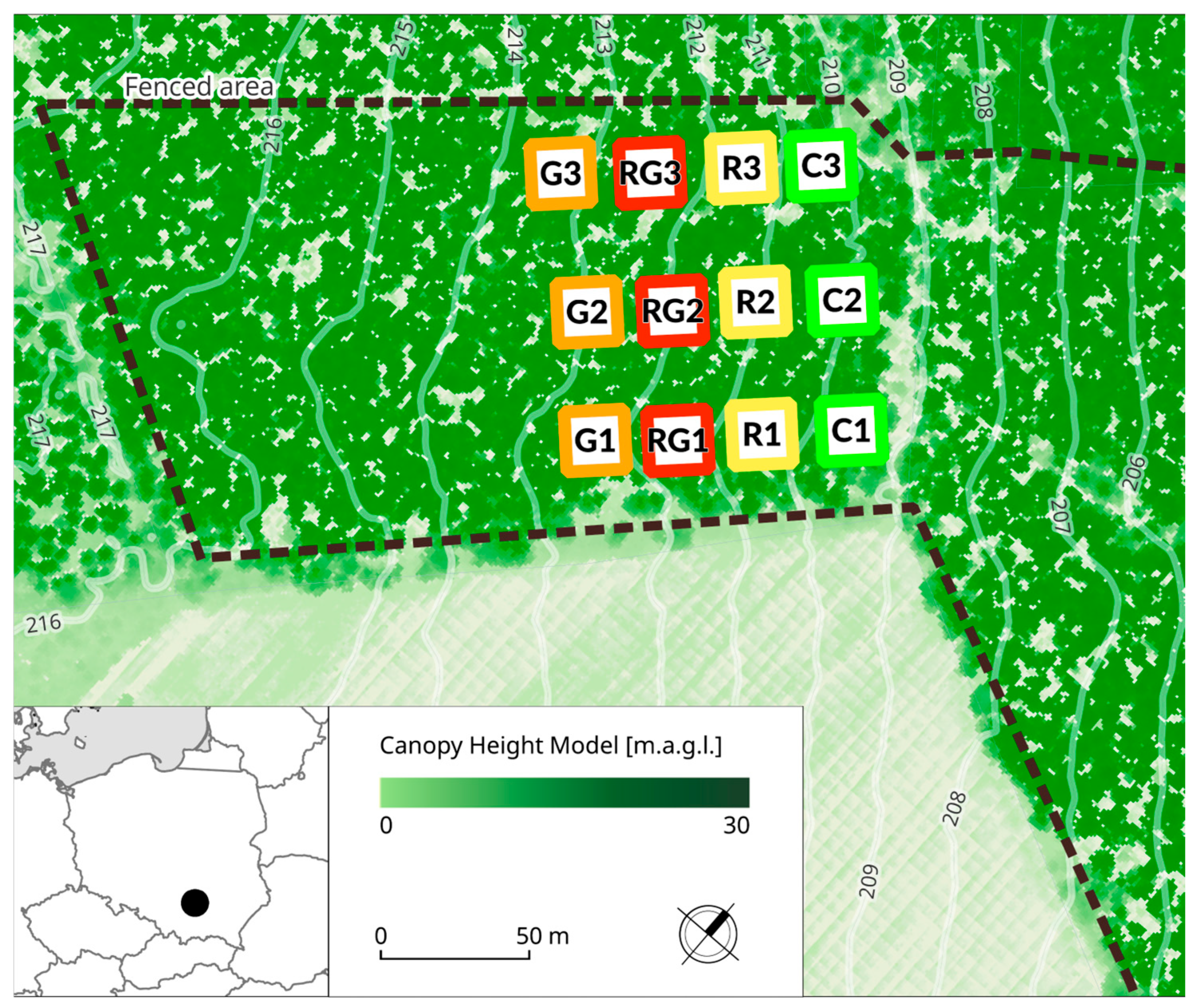
The area was enclosed by a 2.2 m high fence to exclude wild game. Plots were arranged in rows perpendicular to the forest border. The arrangement was systematic rather than randomized; the gradients this creates, and the way they are handled in the analysis, are set out at the end of this section. Control and removal plots were fenced to 0.8 m to exclude sheep; grazing and removal + grazing plots were only marked. Because the thinning was applied to all the area, the control is a reference that includes thinning, not an intact baseline, so all comparisons below are against thinning.
Grazing used a flock of 30 Polish Black-Headed sheep, which grazed the accessible area from late June to late September in 2016, 2017 and 2018. Stocking density was approximately 1.0–1.3 sheep ha−1 yr−1, considered moderately low for forest pasture [39,60]. Shrub removal was performed annually in mid-June with brush cutters.
Vegetation was recorded on 50 randomly placed 1 m × 1 m subplots within each of the twelve plots, giving 600 subplots per survey. One baseline survey was carried out in early June 2016, before any treatment, and the post-treatment survey was made in early June 2019, after three cycles of management. Subplots were positioned independently on each occasion, so the two surveys are not repeated measurements of the same square meter but two independent samples of the same plot. Thus, 1200 subplot records were obtained in total.
The spatial arrangement of plot variants was consecutive rather than randomized, for practical reasons: the same west-to-east sequence (grazing, removal + grazing, removal, control) was repeated in each of the three rows. Two environmental gradients were identified in the field. The forest–field boundary runs parallel to the plot rows and is orthogonal to the treatment arrangement; so, it was accounted for by constraining permutations within rows in all tests below. The second gradient, a mild elevation decrease of about 5 m toward the north-east, runs largely along the treatment axis. The site lies roughly 24 m above the Nida valley floor and 1400 m from the nearest watercourse, so this offset is not expected to translate into a moisture gradient. More importantly, because each variant is assessed as the change in herb layer between its 2016 and 2019 states rather than by its absolute final state, any time-invariant spatial effect should cancel out and should not distort the detected changes.
The experiment monitored a small part of a larger active-conservation project (3.3 ha of 62.9 ha) funded under the European Commission’s LIFE+ Programme (see Funding). Grazing followed national and EU regulations, and all required permits and animal-welfare approvals were obtained before the project began. Fieldwork was carried out with the consent of the state land manager, the State Forests—National Forest Holding. No plant specimens were collected; all species were identified in the field, and none is listed on the IUCN Red List.
2.3. Data Preparation
All plant names were standardized to the World Flora Online [61] checklist using the WFO package [62]. Species occurrence data from the 1200 subplots were consolidated into a single dataset.
Each taxon was assigned a life form [63], a life strategy [64], phytosociological preferences [65,66], forest-density preference [67], Ellenberg-type indicator values for light, moisture, soil reaction and nutrients [68], and disturbance, mowing and grazing indicators [69]. These were merged with the experimental observations (2016, 2019), the forecast states (2028) and the reference relevés of Potentillo albae-Quercetum and Tilio-Carpinetum [70] into one table, which served as the input for all subsequent calculations.
Indifferent species in the system of Tichý et al. [68] were excluded from the denominator of the community-weighted mean for the indicator concerned, so that indifference cannot bias the mean downward. Species with no value were excluded in the same way. The disturbance, mowing and grazing indicators of Midolo et al. [69] contain no indifference code, so they were taken as published and rounded to the nearest 0.05 when the trait table was compiled.
2.4. Statistical Analysis
2.4.1. Species Turnover
Turnover between 2016 and 2019 was described by classifying each taxon as disappeared, persisting or new, and by recording the change in species number and cumulative frequency for each variant.
Direction of frequency change was summarized separately. For each species, frequency was expressed as the number of occupied subplots pooled across the three plots of a variant (0–150). Comparing 2019 with 2016, each species was assigned to one of five mutually exclusive categories: appeared, disappeared, increased, decreased, or stable. Each species was classified once per variant, so each taxon contributes to a single category per treatment. This descriptive partition complements the inferential analyses below and was not itself subjected to significance testing.
2.4.2. Functional Groups, Community-Weighted Means and the Level of Inference
Community-weighted means (CWM) were computed for each subplot. Subplots, however, were re-randomized between surveys and share a single treatment application within each plot. Thus, subplots are not independent experimental units, whereas the plot is. Treating the species or the subplot as the unit inflates the effective sample size roughly thirtyfold and produces very small p-values for very small effects.
We therefore averaged subplot CWM values within each plot and survey year and tested the 2016 → 2019 change on the resulting twelve plot-level differences with an exact sign-flip permutation test, enumerating all 212 = 4096 sign assignments. Differences between variants were tested by permutation ANOVA on the same plot-level differences (9999 permutations of the variant labels, fixed seed). All inferential statements about trait change (presented in Section 3.3) refer to these plot-level tests (Table S1). With three replicates per variant, this comparison has low statistical power, so between-variant contrasts should be interpreted as consistent patterns, rather than thoroughly tested differences.
For completeness, changes in the frequency of functional groups and in community-weighted trait values were also tested within each variant at the subplot level using Fisher–Pitman permutation tests (oneway_test, package coin, 9999 permutations [71]), with the species as the unit of analysis weighted by its number of occurrences. Categorical traits (life form, life strategy, vegetation-type preference, forest affinity) were coded as binary membership variables; whereas continuous indicators were tested directly. These results are retained as a descriptive summary of the full dataset (Table S2).
2.4.3. Ordination and Environmental Drivers
Non-metric multidimensional scaling (NMDS; metaMDS, package vegan [72]) was used at three scales. First, a micro-scale ordination of the binary presence–absence matrix of all 1200 subplots. The number of dimensions was chosen from a stress scan over k = 2–9 (stress = 0.321, 0.249, 0.204, 0.174, 0.152, 0.134, 0.120 and 0.108, respectively). We retained k = 6, the lowest dimensionality at which stress fell below 0.16 and beyond which each further dimension reduced stress by less than 0.02. Second, an independent two-dimensional ordination restricted to the experimental plots was used to visualize treatment-specific successional paths. Third, a consolidated reference ordination (2D) benchmarking the experimental and forecast trajectories against the reference relevés was used. Here, a chord transformation (decostand, method normalize) [73] preceded the Bray–Curtis dissimilarities (stress 0.165, Table S14), and this unified space is the sole framework for the community panorama and the convergence metric.
Differences in composition between 2016 and 2019 were tested by permutational multivariate analysis of variance (PERMANOVA [74]; adonis2, vegan) on Bray–Curtis dissimilarities with 999 permutations. For the overall test and for each variant, permutations were restricted within plot rows; per-variant tests used 300 subplots. The same test was run separately for each of the twelve plots (n = 100 per plot), unconstrained, since no spatial stratification applies within a single plot. Homogeneity of multivariate dispersion was checked with betadisper [75]. The significance of treatment and year as global factors was assessed by fitting them onto the ordination (envfit, 999 permutations). To test whether the projected trajectories continue the experimental ones, the experimental phase was contrasted with the forecast phase by PERMANOVA on Sørensen (presence/absence) dissimilarities (n = 60; 999 permutations).
Functional and environmental drivers were identified by fitting vectors onto the first two axes of the micro-scale ordination. These indicator vectors serve as proxies for the underlying management drivers rather than as the drivers themselves. Significance and directional strength were assessed by 999 permutations (envfit), with vector lengths scaled by √R2. For display, the configuration and vectors are shown on the first two axes, which capture the dominant compositional gradients. Because NMDS axes are not ranked by explained variance, these two axes serve as an interpretive cross-section while the remaining dimensions capture finer structure that stabilizes the configuration without altering the main gradients. Ninety-five percent confidence intervals for the reported effect sizes were obtained by nonparametric bootstrap with a fixed seed (1999 resamples for the trait and dispersion statistics, 999 for the envfit R2 and 499 for the PERMANOVA R2).
Because subplots were re-randomized between surveys and share one treatment application per plot, this subplot-level test is reported as a description of compositional turnover within plots and not as a comparison between treatments; restricting the permutations within rows limits the spatial gradient but does not remove the nesting. Treatment-level inference was therefore made on the twelve plot-level frequency vectors: the survey effect by enumerating all 212 = 4096 flips of the two survey labels within plots, and the grazed/ungrazed contrasts by enumerating all 924 six-against-six splits of the twelve plots and, with row position held constant, all 216 within-row splits (Table S15).
2.4.4. Succession Forecast
Vegetation dynamics were simulated to 2028 with a multi-step ensemble forecast using the caret package [76]. Five learners were trained under identical five-fold cross-validation: random forest (ranger [77]), stochastic gradient boosting (gbm [78]), a generalized linear model (glm [79]), a single-hidden-layer neural network (nnet [80]) and a rule-based regression model (Cubist [81]). Models were trained on the observed turnover (2016–2019) with ten predictors: the treatment variant and the species identity, both entered as factors; the species’ baseline frequency (Freq16); a dynamic Local Context Frequency (LCF); the four Ellenberg-type indicator values; and the mowing and grazing indicators. The remaining traits used elsewhere in the study (life form, life strategy, phytosociological preference, forest-density preference and the two disturbance indicators) were not used as predictors.
Species lacking an Ellenberg-type value for one of the four indicators were given the pool median for that indicator in the machine-learning step only; this affected 97 values across 72 species and does not enter the community-weighted means.
The model extends the single-species historical-proximity framework of Mędrzycki et al. [82] to a saturated, community-level setting. Freq16 carries the historical-proximity signal, while the LCF—the mean frequency of co-occurring species in the same plot, recomputed at each forecast step—enters as a largely independent community-background term (Pearson r = −0.20 with Freq16; n = 1500), representing local saturation rather than a species’ own trajectory.
The simulation ran through three three-year cycles (2022, 2025, 2028) with recalculation of the LCF at each step. Final projections used a single consensus mean per variant and year, to limit the bias of any one algorithm. To gauge robustness, we recorded the minimum–maximum spread of the predicted group share across the five learners for each variant, vegetation group and forecast year. This between-model spread quantifies structural disagreement around the consensus; and it is not a full predictive interval, because it excludes residual variance and the accumulation of error across recursive steps. The projections are accordingly interpreted as indicative trajectories rather than predictions.
2.4.5. Convergence to the Reference Communities
The restoration target was defined as the species composition of Potentillo albae-Quercetum based on contemporary relevés [70], with Tilio-Carpinetum as the contrasting, non-target reference. Within the consolidated reference ordination, each plot’s Euclidean distance to the reference centroid was computed for 2016, 2019 and 2028, and convergence was expressed as the reduction in that distance, Δd = d2016 − d2019 for the observed phase and d2019 − d2028 for the forecast phase. Positive values indicate movement toward the reference state. The reference set comprises 164 relevés—83 of Potentillo albae-Quercetum and 81 of Tilio-Carpinetum—each community represented by a historical and a contemporary group [70]. The restoration target is defined by the contemporary Potentillo albae-Quercetum relevés alone, of which 23 of the 26 available were used; the three omitted did not meet the criterion of forest, having been recorded in field copses with a young tree layer.
These relevés differ from ours in the way species quantity is recorded: they use a cover-abundance scale on plots of 400 m2 or 100 m2, whereas our values are frequencies among 1 m2 subplots. We are aware of this difference and do not treat the resulting distances as measurements on a common absolute scale. What the comparison supports is the direction in which our plots moved relative to a fixed reference configuration, and the relative magnitude of that movement between variants; it is used only in that way. We searched for reference material sampled comparably to the experimental plots and found none better suited than the relevés used here.
Convergence was computed for both phases: for the observed phase from the 2016 and 2019 configurations, and for the forecast phase from the 2019 and 2028 configurations, so that the projected continuation of each trajectory is expressed on the same scale as the measured one.
2.5. Software and Use of AI Tools
All analyses were carried out in R (v. 4.6.1) [79] and the study-area map was prepared in QGIS (v. 4.2.3) [59]. Data handling and graphics used the tidyverse collection [83], with ggrepel, patchwork, scales and ggnewscale for figure composition, and doParallel for parallel processing. The complete computational environment, including package versions, is reported (Table S3; sessionInfo()).
Generative AI assistants were used at three stages of this work, and their use is itemized (Table S4). First, Gemini Pro 3.1 (Google) and Claude Opus 4.8 (Anthropic) were used to help develop and debug the R code for the analyses and visualizations reported here, and for language editing of the manuscript. Second, Claude Opus 5 and Claude Opus 5.5 (Anthropic) audited that code and implemented the corrections together with the plot-level permutation test of Section 2.4.2, the convergence metric of Section 2.4.5 and the additional analyses requested during peer review. The authors verified every correction against the original indicator-value source [68], re-ran the full pipeline on their own data, and checked all affected tables and figures against the previous outputs. The study design, the choice and parameterization of all analytical methods, and the interpretation of all results were carried out by the authors alone. All code was run by the authors on their own data, and no data, results, figures or tables were generated by generative AI tools. Third, Claude Opus 5 and Claude Opus 5.5 (Anthropic) were used to correct the language of the text.
3. Results
3.1. Species Richness and Turnover
Before the experiment, 125 species with 7865 occurrences were recorded in the herb layer of all plots together. Frequencies above 75% were reached by Anemonoides nemorosa, Viola reichenbachiana, Convallaria majalis, Quercus robur and Galium odoratum. Per variant, the control held 79 species with 1995 occurrences, shrub removal 96 species with 1974, grazing 86 species with 1953, and removal + grazing 97 species with 1943.
After three years, both the number and the frequency of species were higher in every variant. In total, 132 species with 10,457 occurrences were recorded in 2019, with Poa nemoralis, Lathyrus vernus and Geum urbanum joining the group above 75%. The strongest change occurred under removal + grazing variant and the weakest in the control (Table 1).
Table 1.
Change in the frequency of occurrence of the herb-layer species recorded in more than 100 subplots in total, between 2016 and 2019, by treatment variant. Values are percentage points of the 150 subplots surveyed per variant and year (three plots × 50 subplots). Species are ordered by their total number of occurrences across both surveys.
Composition shifted in the same direction in every variant, but the imbalance between gains and losses widened with the intensity of intervention. Classifying each species by the direction of its frequency change (Figure 2), the dominant signal in all variants was an increase in the frequency of species already present rather than wholesale turnover (40, 49, 52 and 52 species increased in the control, removal, grazing and removal + grazing conditions, respectively). Newly appearing species showed the clearest treatment gradient (14, 19, 28 and 28, respectively), whereas losses were comparatively flat (8–12 species disappeared; 17–24 declined). Gains exceeded losses in every variant, most strongly under grazing and removal + grazing (80 vs. 27 and 80 vs. 35) and least in the control (54 vs. 29). Tree and shrub species dominated the losses across the board, while the strongest increases were recorded among thermophilous and grassland herbs (Table 1 and Table S5; Figure 2).
Figure 2.
Direction of frequency change between 2016 and 2019: (A) Number of species per category; (B) The corresponding numbers of occurrences lost and gained.
Per plot, the mean number of species gained rose monotonically across the treatments (12.3, 23.7, 26.3 and 30.7 in the control, removal, grazing and removal + grazing variants), while the number lost varied little (8.0–10.0), giving net gains of 4.3, 14.0, 17.0 and 20.7 species. Total occurrences per plot rose by 134, 225, 246 and 259, respectively; and the two grazed variants together gained significantly more occurrences than the two ungrazed ones (exact permutation test on the twelve plot-level gains, grazed vs. ungrazed, p = 0.017).
3.2. Species Composition
The NMDS ordination showed relatively high within-variant variation before treatment. After three years, plots of the same variant converged and shifted away from the controls, the largest mean shift occurring under removal + grazing.
All variants, including the control, changed significantly between 2016 and 2019 (p = 0.001; Table S6). The coefficient of determination, though small, ordered the treatments consistently: control R2 = 0.0223 (F = 6.81), removal 0.0298 (F = 9.15), grazing 0.0429 (F = 13.36) and removal + grazing 0.0582 (F = 18.42)—the last, 2.6 times that of the control. All twelve plots changed significantly (p ≤ 0.012; Table S7), with the most pronounced shifts under removal + grazing and grazing. In the global model, survey year and treatment together explained 7.3% of the variation (F(7, 1192) = 13.34, p = 0.001), with year (r2 = 0.054) slightly stronger than treatment (r2 = 0.041; both p = 0.001).
These subplot-level coefficients order the variants, but they are not a comparison between treatments. At the plot level, the survey explains 14.6% of the variance (pseudo-F = 8.94, exact p = 0.0005); the magnitude of compositional change differs between grazed and ungrazed plots (0.3517 against 0.2679, exact p = 0.0108), while its direction does not separate them at this sample size (pseudo-F = 1.45, exact p = 0.0866; Table S15).
Multivariate dispersion also differed significantly between surveys (betadisper, F = 151.64, p < 0.001), decreasing between 2016 and 2019: the mean distance to the group centroid fell from 0.362 to 0.310, and the decrease was consistent across all four variants (Table S6).
Fitting the indicator variables onto the ordination identified the nutrient indicator as by far the strongest correlate of composition (R2 = 0.379, 95% CI [0.335, 0.424]), followed by soil-reaction indicator (0.246 [0.199, 0.292]), disturbance severity indicator (0.141 [0.106, 0.184]) and soil-moisture indicator (0.078 [0.052, 0.112]); all eight variables were significant at p = 0.001 (Table S8). Grazing (0.073 [0.044, 0.108]), light (0.030 [0.014, 0.053]), mowing (0.028 [0.012, 0.052]) and disturbance frequency indicators (0.018 [0.006, 0.039]) were significant but weak. The confidence intervals of nutrients and reaction do not overlap those of the remaining variables, indicating that composition along the leading ordination axes tracked the soil trophic–reaction complex rather than a moisture gradient, which was not manipulated in this experiment (Figure 3).
Figure 3.
Ordination of herb layer species of the 1200 subplots by NMDS method with the fitted indicator vectors (fitted with envfit function of vegan package). Vector lengths are scaled by the square root of R2.
3.3. Functional Traits and Community-Weighted Means
At the plot level (n = 12), the herb layer shifted toward more light-demanding (ΔCWM light = +0.088, p = 0.025), somewhat more drought-tolerant (moisture = −0.049, p = 0.002) and distinctly less nutrient-demanding species (nutrients = −0.109, p = 0.031), together with an increase in the disturbance-frequency indicator (+0.009, p = 0.004) and the mowing indicator (+0.009, p = 0.009). Soil reaction showed no significant directional change (+0.029, p = 0.121), nor did disturbance severity (+0.004, p = 0.178), and the grazing-tolerance indicator increased only marginally (+0.001, p = 0.078) (Table S1).
These tests compare 2019 with 2016 across the experiment as a whole; and they do not compare the four variants with one another. A separate permutation ANOVA on the plot-level changes gave no significant differences between variants for any indicator (all p > 0.22, Table S1), which is expected with three replicates per variant. The ranking of variants is therefore reported as a consistent pattern, not as a tested contrast. For nutrient demand, the plot-level change was monotonic across the intensity of intervention (control −0.041, removal −0.078, grazing −0.133, removal + grazing −0.182), consistent with hypothesis 1, although the between-variant test was not significant.
At the subplot level (Table S2), where the larger sample allows finer resolution, gains in thermophilous oak-forest species were significant in all three active treatments and absent in the control (p = 0.002, 0.001 and 0.002 against p = 0.95). Gains in grassland species were significant in every variant, the control included (p = 0.022), so that group does not separate the treatments from the thinned baseline. Among the functional groups, mixed-CSR strategists gained significantly only under grazing and removal + grazing, and hemicryptophytes only under removal and removal + grazing. The disturbance-frequency indicator rose significantly in the control as well as in the treated plots, the mowing indicator in every variant except grazing (p = 0.076, Table S2), and the disturbance-severity indicator only under removal; none of the three is therefore specific to grazing.
Species typical for thermophilous oak forests approximately doubled their frequency in all three active treatments, while increasing only slightly in the control. Among them, the dominant role was played by Lathyrus niger, Astragalus glycyphyllos and Melittis melissophyllum (Table S9). Per plot, occurrences of the thermophilous forest species (Table S11) rose by 10.3, 37.7, 43.0 and 38.7 in the control, removal, grazing and removal + grazing variants. And the grazed variants did not differ significantly from the ungrazed ones on this subset alone (p = 0.115). By 2019, the thermophilous forest species formed 8.0%, 9.2%, 10.1% and 8.8% of the occurrences (Table S11) in the control, removal, grazing and removal + grazing, respectively.
Critically, none of the three characteristic species for Potentillo albae-Quercetum (i.e., Lathyrus niger, Astragalus glycyphyllos and Melittis melissophyllum) appeared in a plot where it had been absent in 2016: all three were present in all twelve plots at the baseline, and their entire gain consists of increased frequency of resident populations. Across the wider group of 18 thermophilous species, the same pattern dominates, and the proportion of the gain attributable to newly appearing species did not differ between grazed and ungrazed variants (16.6% vs. 14.8%, p = 0.77).
3.4. Forecast
Changes projected over the nine years following the experiment follow the same direction as those observed during it. The projected phase differs highly significantly from the experimental phase (PERMANOVA: F(1, 58) = 70.56, R2 = 0.549, 95% CI [0.474, 0.653], p = 0.001).
The largest changes are projected under removal + grazing, with similar magnitude under grazing and the smallest in the control. Projected change slows in intensity despite the longer horizon, and the final states converge across all variants, including to some extent, the controls (Figure 4).
Figure 4.
Successional trends for the twelve plots, observed (2016–2019) and projected (2022–2028), using an ensemble forecast based on the historical proximity method.
All five learners showed consistent cross-validated performance for the one-step transition (2016 → 2019): R2 = 0.889–0.937, RMSE = 0.064–0.085, MAE = 0.036–0.054 (Table S10). The generalized linear model performed best (R2 = 0.937 [0.926, 0.948]; RMSE = 0.064 [0.061, 0.068]).
Although the absolute frequency of species from almost all vegetation groups increased in every variant, their percentage shares moved differently, both in the experiment and prediction. The share of grassland species rose in every variant and at almost every step. The share of thermophilous oak-forest species rose in the three treated variants but not in the control, where it was unchanged. Forest-edge species lost share in the experimental phase in all four variants; in the forecast, the decline continued in the control and under removal + grazing, while removal and grazing recovered a small fraction of the loss. The synanthropic species share—the smallest of all—fell slightly during the experiment and rose slightly in the forecast (Table S11). Species of half-shaded forests lost share in every variant during the experiment, and the projection continues that decline without interruption in all four.
The projected trends were robust to the choice of algorithm: the between-model spread was 4 to 13% of the group mean in five of the six vegetation groups (median 1.28, maximum 3.33 percentage points), with larger divergence only at the single-species level (Table S14) and in the synanthropic group, whose share stays below 1%. Across treatments, projected increases were dominated by thermophilous and shaded forest herbs and decreases by forest edge (mainly woody and shrub) species, most strongly under removal + grazing (Figure 5).
Figure 5.
Share of species associated with each vegetation group, observed and projected. Panels: C—control, R—shrub removal, G—grazing, RG—shrub removal with grazing. Whiskers show the minimum–maximum spread across the five applied learners.
3.5. Convergence to the Reference Communities
The experimental plots occupy a region of the consolidated ordination distinct from both reference communities, lying below them on the second axis throughout the study. Their position is nevertheless asymmetric: at the baseline, the centroid of the twelve plots lay closer to the contemporary relevés of Potentillo albae-Quercetum than to those of Tilio-Carpinetum (1.20 against 1.77 ordination units), so the stand entered the experiment already on the thermophilous side of the reference space. Both reference communities are themselves displaced between their historical and contemporary relevés, and in different directions, so convergence is assessed against their contemporary state (Figure 6).
Figure 6.
Community panorama: the experimental and projected plots placed against the historical and contemporary relevés of the two reference communities by NMDS method (metaMDS, of vegan package) with a chord transformation (decostand, method “normalize”) preceding the Bray–Curtis dissimilarities.
Between 2016 and 2019, the plots moved as a group toward Potentillo albae-Quercetum, and the projected trajectories toward 2028 continue in the same direction. The mean plot distance to that reference falls from 1.20 to 1.09, and to 0.97 by 2028, whereas the distance to Tilio-Carpinetum falls more slowly, from 1.77 to 1.71 and 1.62. The ratio between the two widens accordingly (1.48, 1.57, 1.67), indicating movement preferentially toward the thermophilous reference rather than merely away from the starting position.
During the observation period, the two grazed variants converged on Potentillo albae-Quercetum to a similar degree (removal + grazing Δd = 0.168; grazing Δd = 0.159), between about 1.8 and 4.1 times the convergence of shrub removal alone (0.091), depending on the space in which the distance is measured, and an order of magnitude greater than the control (0.015); the ratio is given for six such configurations in Table S16. Convergence toward Tilio-Carpinetum was weaker throughout (0.106, 0.117, 0.030 and −0.015, respectively), confirming that the trajectory was directed toward the thermophilous rather than the mesic reference community (Figure 7).
Figure 7.
Convergence to the reference forest communities, expressed as the reduction in distance to the reference centroid (Δd). Intense-colored segments represent the observed phase (2016–2019), while pale-colored segments, the projected continuation (2019–2028); positive values indicate movement toward the reference state. C—control, R—shrub removal, G—grazing, RG—shrub removal with grazing. Each bar is the mean of three replicate plots.
The three replicate plots behind these means were not equally consistent. Under grazing, the response ranged from 0.031 to 0.236 (SD 0.112), the variant mean resting on two of the three plots, whereas removal + grazing gave 0.135, 0.137 and 0.232 (SD 0.056). The control was the least variable and the least responsive (SD 0.033).
In the forecast phase, the ranking reverses: the control shows the largest projected further convergence (0.202), ahead of shrub removal (0.113), removal + grazing (0.094) and grazing (0.070).
4. Discussion
4.1. What This Experiment Design Can and Cannot Show
Several features of the design of the experiment, carried out alongside the large Life+ restoration project, set the terms on which its results should be read. Because the same west-to-east sequence of treatments was repeated in all three rows rather than randomized within them, treatment is aliased with position along the row, and no difference between two variants can be read as an effect of treatment alone. Re-drawing the subplots at each survey rules out following an individual square meter through time, and with it, any spatially explicit account of canopy gaps or immediate neighbors. Three plots per variant limit how finely the four treatments can be told apart. Finally, the three-year duration limits both which processes can appear at all and how far their effects can be followed.
Although these features make the experiment results less mechanistic than a randomized trial would allow, the results still hold substantial potential for practical applicability in thermophilous oak forest management. What the design answers is whether three years of shrub removal and reintroduced grazing move the herb layer of a neglected oak forest toward its nominal composition, and in which direction its functional makeup shifts.
What the layout does not affect is change within a plot: each plot is compared with itself, so its position, its elevation and its soil enter both surveys equally and cancel. Re-drawing the subplots at each survey trades one kind of information for another. Consequently, each survey is a fresh sample of the whole plot, so the plot-level frequencies describe the plot rather than one fixed and possibly unrepresentative set of squares.
With three plots per variant, differences between individual variants are consistent in direction but we present them as patterns rather than as tested effects. We tested the positional objection directly rather than only arguing from the design. Six covariates measured before the experiment by the 2012 airborne survey—elevation, slope, mean canopy height, canopy closure, gap fraction and stem density—were related to three measures of change: convergence, the gain in occurrences and the gain in thermophilous occurrences. Between variants, the covariates track treatment closely, as the layout implies (|r| = 0.56 to 0.99). Within variants, where treatment is held constant, none of the eighteen combinations approaches significance (exact p = 0.10 to 0.88), and the twelve plots would have resolved correlations of |r| = 0.46 to 0.87 at the 5% level (Table S17). Position, therefore, does not account for the changes reported here, with the caveat that three plots per variant make this a weak test rather than an exclusion. Grouped into grazed and ungrazed, the comparison does carry weight, and our conclusion about grazing rests on it (p = 0.017).
Some treatment effects in thermophilous oak forests take longer to express themselves, and others fade: e.g., light-demanding species disappeared after ten years in a Czech restoration project of the same community type [45]. Three years were enough to resolve the direction of change, which is what we claim, but insufficient to establish its persistence, which we do not.
Taken together, these features make the experiment less mechanistic than a randomized trial would allow, but they do not reduce its practical value for thermophilous oak forest management. What the design answers is whether three years of shrub removal and reintroduced grazing move the herb layer of a neglected oak forest toward its historical composition, and in which direction its functional makeup shifts. It cannot establish which of the two types of interventions contributes more. Both would need a larger, randomized trial, and what this one shows is that the direction is real enough to justify it.
4.2. Thinning as the Shared Baseline
The most consequential feature of this experiment is that every plot, including the control, was thinned in 2015. The control therefore measures the effect of thinning alone, and every comparison reported here is a comparison against a stand that has already been opened.
This explains the otherwise puzzling result that composition changed significantly even in the control (R2 = 0.0223, p = 0.001). Thinning stimulates the undergrowth [84,85,86], though the effect usually declines within three to four years [45]. A meta-analysis of North American experiments that separated thinning from burning reports the same short-lived release, with a caution worth repeating here: the two are not interchangeable, and thinning alone tends to favor non-native and ruderal species [87], and the extraction of felled trees disturbs the forest floor, creating germination sites that favor therophytes and ruderals [88,89,90]. Both processes operated in all twelve plots. The shrub layer these treatments act on is an instance of a pattern described worldwide: once a dense understory layer establishes, it suppresses regeneration and herb-layer diversity and persists until something removes it, which is why a single removal is not enough and why the regrowth we recorded was to be expected [91]. The indicator values bear this out in a way that is easy to miss: the plot-level increase in the light indicator was largest in the control (+0.132) and smallest under removal + grazing (+0.019), and at the subplot level, it was significant only in the control (Table S2). The ranking of the treatments therefore does not follow the lightindicator, which is what one would expect if thinning had already saturated it. It also reframes what the treatments were being asked to do. Light was not the limiting factor in this experiment, because thinning had already released it everywhere. Directional change occurred in every variant: its direction was the same in all four, and the treatments altered its rate and the distance travelled rather than whether it occurred. The control is the clearest case, since it received only thinning and still moved. What a single local control establishes is bounded: it fixes the background change at one site in one stand and cannot separate the change a stand would have undergone anyway from the regional trends in deposition, climate and herbivory that act on every plot alike. Networks of long-term platforms turn such a bound into a calibrated baseline. Early-successional platforms show that structure in a developing community emerges in phases driven by particular species rather than smoothly [92]; multi-site plantation experiments are designed so that site is a factor rather than a confounder [93]; and a synthesis of 39 European resurvey studies, drawing on almost four thousand records taken 17 to 75 years apart, found no net loss of local plant diversity but wide variation between sites, traced to drivers that operate at different scales—change in light availability locally, the density of large herbivores regionally, with nitrogen deposition before the first survey predicting the later change [94]. This experiment manipulates light and herbivory together at one site and under one deposition history, so it speaks to the local term and not to the regional one.
What distinguished the treated plots from the control was the removal of shrub-layer biomass and litter, and—under grazing—trampling, selective herb layer grazing and local nutrient redistribution. The consistent decline in plants of high nutrient demand across all variants, steepest where intervention was most intense (−0.041 to −0.182), is the signature of that biomass export rather than of light release.
An untreated control would have answered a different and equally interesting question, and its absence is the main design limitation we would remove if the experiment were repeated.
4.3. Grazing as the Clearest Contrast
Across every criterion taken into consideration, the two grazed variants separate from the two ungrazed ones more clearly than any other contrast. Grazed plots gained significantly more occurrences (p = 0.017). They converged on the target community more strongly than shrub removal alone under every one of the convergence metrics examined (Table S16) and roughly an order of magnitude more than the control; and their herb layer carried the larger declines in nutrient demand.
What they do not show is an advantage of combining the two treatments over grazing alone. Removal + grazing converged marginally further than grazing (0.168 vs. 0.159), but the difference is about 6% of the effect and cannot be tested at this sample size. Hypothesis 2 is therefore only partly supported: the direction of the gradient matches the prediction, and grazing is clearly the component that matters, but the increment from adding shrub removal to grazing lies within the noise of this design. This also qualifies, without contradicting, our earlier single-season finding that the combination gave no additional benefit [53]: over three years, the combination is at least as effective as grazing alone, and possibly slightly more so, but the evidence does not support presenting it as the superior treatment.
The mechanisms by which grazing could act are well established—selective herb layer grazing, trampling that breaks the litter layer and exposes germination sites, local fertilization, and seed transport in fleece and dung—and shrub removal provides none of them beyond the first. The functional responses are coherent with community-assembly theory: the rise of hemicryptophytes and the dominance of mixed CSR strategists [64] is what is expected of a system released from competitive exclusion, where moderate recurrent disturbance favors species combining competitive ability with tolerance of stress and disturbance.
4.4. Release Rather than Recruitment
None of the three characteristic species of Potentillo albae-Quercetum appeared in any plot where it had been absent. All three were present in all twelve plots in 2016, and their entire gain—which approximately doubled their frequency in the active treatments—consists of resident populations becoming more frequent. Across the broader group of 18 thermophilous species, the share of the gain contributed by newly appearing species was indistinguishable between grazed and ungrazed variants (16.6% vs. 14.8%, p = 0.77). Grazing raised both recruitment and release across the whole flora in roughly equal proportion. For the wider flora, however, this comparison has a limit that the three characteristic species do not share: because the 1 m2 subplots were relocated between surveys rather than permanently marked, a species recorded in 2019 but not in 2016 may have been present in the plot all along, outside the 2016 subplots. The claim that the gain came from release rather than recruitment is therefore firm for the three characteristic species, which were present in every plot at baseline, and is offered as the more likely of two readings for the rest, as it did not selectively recruit target species.
Two readings are possible, and the data here cannot separate them. The first is that the barrier to restoration at this site was not dispersal but competition and shading, which is why three years sufficed to produce a measurable response in resident populations. The second is that three growing seasons are simply too short for recruitment to become visible: seedlings of some perennial forest herbs may need more years to reach a stage at which they are recordable in a relevé. Both readings point to the same practical conclusion for a three-year horizon—the measurable gain comes from releasing what is already present—but they differ in what to expect later, and distinguishing them would require a longer series of surveys.
A treatment that releases residents can only release what is present. In this stand, the thermophilous signal rests almost entirely on three species, which together account for roughly three-quarters of the group’s occurrences (71–84% in 2019, depending on variant); of the remaining fifteen, the most frequent reached twenty-two records out of 150 and most stayed in single figures. Peucedanum cervaria, a characteristic species of the association, was recorded once in the entire experiment—a single subplot in the control in 2016—and not again. Whether this reflects a genuine qualitative impoverishment of the local flora or the limits of a three-year window cannot be settled here, and we note it as an open question rather than a diagnosis.
4.5. Why the Criteria Rank the Treatments Differently
The treatments do not rank identically under all the measures used here, and the discrepancies are informative rather than contradictory, because the measures quantify different things.
The coefficient of determination from PERMANOVA measures how far composition moved, without regard to direction. The change in a community-weighted mean measures movement along a single abiotic axis. Convergence measures movement toward a particular point in multivariate space, and therefore discounts displacement that is large but off-target. Removal + grazing leads on the first two—the largest total gain in occurrences (259 per plot), the largest variance explained (R2 = 0.0582) and the steepest decline in nutrient demand (−0.182)—while grazing alone ends with the highest share of thermophilous species (10.1% vs. 8.8%, Table S11).
We resist reading a mechanism into this. The differences involved are small, none survives a between-variant test at n = 3, and the share-based comparison is additionally confounded by its denominator: removal + grazing gained the most occurrences overall, so an equal absolute gain in thermophilous species yields a smaller percentage share. We note the divergence, report both kinds of measure, and draw conclusions only where they agree—which they do on the separation of grazed from ungrazed variants.
4.6. The Forecast and Its Limits
The projected trajectories continue the observed ones in direction, and the narrow spread between the five learners (median 0.07 percentage points, Table S14) indicates that the consensus is robust to algorithm choice. That robustness, however, concerns structural uncertainty alone. The dominant and unquantified source of error is the recursive propagation of uncertainty across forecast steps, which is why the projections are presented as potential trajectories rather than scenarios. Ensemble averaging was adopted for exactly this reason: combining learners of different inductive bias and reporting their consensus limits the influence of any single model specification [76,82,95,96].
The high coefficient of determination of the predicted-versus-experimental comparison (R2 = 0.549) should not be read as a stronger biological effect than the treatment effects (R2 = 0.022–0.058). It largely reflects the temporal autocorrelation of species frequencies, since each forecast step is built recursively from the preceding state. The treatments exert a real but moderate directional influence on the herb layer; they are not dominant drivers of its overall composition, and the remaining variance reflects the fine-scale micro-mosaic of habitat conditions among subplots. The same caution applies to the cross-validated coefficients of determination of the individual learners (R2 = 0.889–0.937, Table S10): since species identity enters the model as a factor, they may largely reflect the persistence of species-specific frequency levels between the two surveys and should not be read as the predictive power of the trait terms alone.
A further limitation of the forecast is structural rather than statistical. The entire community context of a projected transition rests on one predictor, the mean frequency of the species co-occurring with the focal species in the same plot. That single term compresses the whole competitive neighborhood into an average, so the identity of a species’ competitors—e.g., which of them shade it, which share its rooting depth, which are palatable to sheep—is not represented. Nor is the physical micro-site: because subplots were re-randomized between surveys rather than permanently marked, the design carries no spatially explicit record of canopy gaps, crown projections or immediate neighbors, and the model cannot condition on them. Both simplifications act in the same direction, removing sources of among-site heterogeneity from the predictors, and a forecast built on averaged context will tend to produce trajectories that are smoother and more alike than the vegetation itself. Thus, the consequence for reading the projections is specific: the direction of change they indicate is supported by the observed phase, but the spread around that direction is likely to be wider in the field than in the projection. One property of the ensemble needs stating plainly, because it governs how the projected shares should be read. The learners return a frequency for every species on every plot and cannot return an absence, whereas almost half of the observed records in 2019 are absences. Where a group is common, this matters little. Where it is not, it matters a great deal: in the synanthropic group, 82% of the observed records are absences, so most of its projected presence is interpolation rather than prediction, and its share—below one per cent throughout—should not be read as a quantity. The projections are therefore to be read for the direction of change and for the relative ordering of the variants, not for the level of any one group in any one year.
4.7. Management Implications and Further Research
In this experiment, the most effective approach combined thinning, shrub removal and grazing, with grazing the component that mattered most. Because of the costs involved, such comprehensive measures are likely to be feasible only within targeted conservation projects.
Properly managed forest herding can generate some revenue. Low-intensity grazing persists locally and is being revived within agri-environmental and restoration schemes [40,97], yet its return to forests at a meaningful scale remains constrained by socioeconomic factors, making its implementation a complex issue [98,99]. Conservation grazing of wood pastures with cattle may even yield a small net profit (£17.25 ha−1 yr−1), comparing favorably with mechanical shrub removal (≈£112.50 ha−1 yr−1 [100]), and tourism can add income in some regions [101]. External subsidies help but do not solve the problem, so maintaining or restoring forest pastoralism remains crucial [102,103,104].
Restoring species-rich thermophilous oak forests through reintroduced grazing forms part of the biocultural management of landscapes [105,106], which uses traditional agriculture to preserve natural values from the species to the landscape level alongside traditional knowledge, customs and social relations [27,28], helping to maintain or restore highly specific local socio-ecological identities [107,108]. This approach is supported by EU legislation on biodiversity, particularly the Nature Restoration Regulation [109], which requires Member States to achieve a positive trend in a range of biodiversity indicators in forest ecosystems. These are long-term activities requiring legal and economic regulation at Union or Member State level.
Against this background, thinning deserves separate consideration, on grounds that come from the economics of forest management rather than from this experiment, which did not test them. As a mandatory, cyclical operation it generates measurable revenue from timber sales. Thinning alone produced the weakest response among the variants, but its cyclical timber revenue can offset the need for conservation funding, so combined with periodic low-intensity grazing, this may be the most viable strategy for large-scale application. Establishing its optimal intensity and return interval, and a minimum stand age to avoid crown deformation, would require provisions allowing it as an optional protective measure in forest management. Provisions permitting limited, controlled forest grazing would be equally worthwhile; such practices continue in some countries despite decades of prohibition [40] and elsewhere are being implemented within research or restoration projects [110].
Three directions for further work follow from the limitations above. First, verification on a larger and more diverse sample, with more replicates per treatment, since the present design cannot sufficiently resolve differences between individual variants. The scale that this question deserves is visible in the North American studies: oak savanna restorations followed for three decades show that the ground layer keeps reorganizing long after the first response [25], and it took replicated multi-site programs to establish that thinning and burning are not substitutes for one another [87]. Three years and three replicates per treatment cannot do that work; they can establish a direction and leave the magnitude to a longer series. Second, inclusion of a control not subject to any preliminary treatment, which would separate the effect of thinning from that of abandonment. Third, monitoring after the cessation of treatments, to establish whether the observed changes persist.
Two more specific questions deserve attention. One is the design of a spatiotemporal mosaic of illuminated patches at landscape scale, which would secure the survival of light-demanding species. Once illuminated, such patches often become feeding sites for deer more frequently than areas under closed canopy, thereby extending their persistence [111], a mechanism that could function similarly to the concept of bright primeval pasture forests [9,49,112]. The other is a systematic assessment of restoring Potentillo albae-Quercetum achieved per unit cost across treatment options by understory removal (timing, frequency, cutting height), grazing (herbivore species, stocking density, duration, rotation), or thinning (stand age, selection criteria, intensity, return interval). Finally, further field observation may help to calibrate the historical-proximity method and improve its ability to emulate temporal change in areas under active protection.
5. Conclusions
- Three years of active management measurably shifted the herb layer of a thermophilous oak forest toward its more characteristic composition. Composition changed significantly in every treatment variant, and the variance explained by the survey year rose monotonically with the intensity of intervention, from 2.2% under thinning alone to 5.8% under shrub removal combined with grazing.
- At the plot level, the herb layer became more light-demanding, less nutrient- and moisture-demanding, and the frequency of disturbance-tolerant species rose.
- Grazing was the component associated with the largest change. Both variants that included it converged on the target community more strongly than shrub removal alone and an order of magnitude more than the thinning-only control, consistently across every way of measuring convergence that we examined. Adding shrub removal to grazing produced no increment that this experiment design can resolve.
- The gain in characteristic species consisted entirely of increased frequency of resident populations. None of them appeared in a plot where it had been absent. The treatments released a suppressed flora rather than recruited a new one, which makes them fast acting where the species pool survives and insufficient where it does not.
- As every plot was thinned before the experiment, all of the above are effects measured against an already semi-opened stand. Thinning alone produced the weakest response of the four variants, but its cyclical timber revenue can offset the need for conservation funding, so combined with periodic low-intensity grazing, it may be the most viable strategy at large scale.
Supplementary Materials
The following supporting information can be downloaded at: https://www.mdpi.com/article/10.3390/f17111299/s1. Table S1: Plot-level community-weighted means: change between 2016 and 2019 per trait, with exact sign-flip permutation tests (n = 12) and between-variant permutation ANOVA. Table S2: Change in the frequency of functional groups and in community-weighted trait values at the subplot level, per variant (Fisher–Pitman permutation tests). Table S3: Computational environment: R version, package versions and session information. Table S4: Declaration of generative AI use: stage, tool, purpose, human verification and effect on the reported results. Table S5: Species turnover by direction of change (appeared, increased, stable, decreased, disappeared) per variant. Table S6: Per-variant PERMANOVA of the 2016–2019 compositional change, with multivariate dispersion (betadisper) and 95% confidence intervals. Table S7: Per-plot PERMANOVA of the 2016–2019 compositional change (twelve plots). Table S8: Indicator variables fitted onto the ordination (envfit): coefficients of determination with 95% confidence intervals. Table S9: Frequency change in the characteristic species of Potentillo albae-Quercetum. Table S10: Cross-validated performance of the five learners used in the ensemble forecast. Table S11: Vegetation-group composition: occurrences and share of each group per variant and survey year. Table S12: Plot-level gains in all species occurrences and in thermophilous oak forest species occurrences, with the exact permutation contrasts between grazed and ungrazed variants. Table S13: The thermophilous oak forest species group: occurrences per variant and year, plots occupied in 2016, including the three characteristic species of Potentillo albae-Quercetum. Table S14: Ordination and model diagnostics: NMDS stress, mean subplot richness, mean distance to the group centroid, the predicted-versus-experimental test, the between-learner spread and the local-context-frequency correlation. Table S15: Plot-level multivariate inference (twelve plots), every grazed/ungrazed contrast under both permutation schemes. Table S16: The convergence metric computed five ways, with the grazed/ungrazed contrast and its exact p in each. Table S17: Positional covariates from the 2012 airborne survey: between-variant and within-variant slopes, with the detectable effect size. Figure S1: Convergence (Δd) against two positional covariates measured before the experiment. Dashed grey line: the slope through the four variant means. Colored segments: the slope within each variant, where treatment is held constant.
Author Contributions
Conceptualization, M.J.-B., T.H., P.M., A.O., A.Ś. and D.P.-M.; methodology, M.J.-B., T.H., P.M. and A.O.; software, P.M.; validation, M.J.-B., A.O., P.M. and D.P.-M.; formal analysis, P.M.; investigation, T.H. and M.J.-B.; resources, T.H., M.J.-B. and A.Ś.; data curation, M.J.-B., T.H., P.M. and A.Ś.; writing—original draft preparation, A.O., M.J.-B., P.M. and D.P.-M.; writing—review and editing, A.O., P.M., M.J.-B., T.H., A.Ś. and D.P.-M.; visualization, P.M.; supervision, M.J.-B., P.M. and A.O.; project administration, M.J.-B. and T.H.; funding acquisition, T.H. All authors have read and agreed to the published version of the manuscript.
Funding
The field experiment was funded by the European Commission LIFE+ Programme, grant no. LIFE13 NAT/PL/000038 (acronym ZSiNPK_Kielce_LIFE_PL), “Protection of valuable natural habitats in Ponidzie”, with a total budget of approximately EUR 1.16 million. The experiment reported here monitored 3.3 ha of the 62.9 ha covered by that project. Grazing was conducted in accordance with national and EU regulations, and the project obtained all required approvals and was supervised by the responsible authorities at European, national, regional and local level. Following completion, the project was approved and settled by the grant provider without reservation, both in 2019 and five years after its closure [113,114,115]. The APC of this paper was supported by grant no. SUPB.RN 099UJK of Jan Kochanowski University of Kielce and co-financed from the funds of KOPIPOL association.
Data Availability Statement
The original data presented in the study—including the subplot × species occurrence matrices for 2016 and 2019, the functional-trait and ecological-indicator table, and the analysis and forecast code—are openly available on Figshare at https://doi.org/10.6084/m9.figshare.32748822 (CC BY 4.0).
Acknowledgments
During the preparation of this manuscript, the authors used Claude Opus 4.8 (Anthropic) and Gemini Pro 3.1 (Google) for the purposes of assisting in the development and debugging of the R code used for statistical analysis and data visualization, and for language editing, and Claude Opus 5 and Claude Opus 5.5 (Anthropic) for the purposes of auditing and correcting that analytical code, implementing the additional analyses requested during peer review, and language editing of the revised manuscript. Each use is itemized in Table S4. The authors have reviewed and edited the output and take full responsibility for the content of this publication.
Conflicts of Interest
The authors declare no conflicts of interest. And the funders had no role in the design of the study; in the collection, analyses or interpretation of data; in the writing of the manuscript; or in the decision to publish the results.
References
- Bürgi, M.; Gimmi, U.; Stuber, M. Assessing traditional knowledge on forest uses to understand forest ecosystem dynamics. For. Ecol. Manag. 2013, 289, 115–122. [Google Scholar] [CrossRef] [Scilit]
- Szabó, P. Driving forces of stability and change in woodland structure: A case-study from the Czech lowlands. For. Ecol. Manag. 2010, 259, 650–656. [Google Scholar] [CrossRef] [Scilit]
- Öllerer, K.; Varga, A.; Kirby, K.; Demeter, L.; Biró, M.; Bölöni, J.; Molnár, Z. Beyond the obvious impact of domestic livestock grazing on temperate forest vegetation—A global review. Biol. Conserv. 2019, 237, 209–219. [Google Scholar] [CrossRef] [Scilit]
- Gillis, R.E.; Kendall, I.P.; Roffet-Salque, M.; Zanon, M.; Anders, A.; Arbogast, R.-M.; Bogucki, P.; Brychova, V.; Casanova, E.; Classen, E.; et al. Diverse prehistoric cattle husbandry strategies in the forests of Central Europe. Nat. Ecol. Evol. 2025, 9, 87–98. [Google Scholar] [CrossRef] [Scilit] [PubMed]
- Szymura, T.H. How does recent vegetation reflects previous systems of forest management. Pol. J. Ecol. 2012, 60, 859–862. [Google Scholar]
- Leuschner, C.; Ellenberg, H. Environmental and historical influences on the vegetation of Central Europe. In Ecology of Central European Forests; Springer International Publishing: Cham, Switzerland, 2017; pp. 3–21. [Google Scholar] [CrossRef] [Scilit]
- Zaniewski, P.T.; Obidziński, A.; Ciurzycki, W.; Marciszewska, K. Past disturbance–present diversity: How the coexistence of four different forest communities within one patch of a homogeneous geological substrate is possible. Forests 2022, 13, 198. [Google Scholar] [CrossRef] [Scilit]
- Bobiec, A.; Reif, A.; Öllerer, K. Seeing the oakscape beyond the forest: A landscape approach to the oak regeneration in Europe. Landsc. Ecol. 2018, 33, 513–528. [Google Scholar] [CrossRef] [Scilit]
- Borkowski, J. Jak wyglądały lasy pierwotne Europy pod presją dużych roślinożerców? [What did European primeval forests under high herbivore pressure look like?]. Leśn. Pr. Badaw. 2011, 72, 183–190. (In Polish) [Google Scholar] [CrossRef] [Scilit]
- Czyżewski, S.; Svenning, J.-C. Temperate forest plants are associated with heterogeneous semi-open canopy conditions shaped by large herbivores. Nat. Plants 2025, 11, 985–1000. [Google Scholar] [CrossRef] [Scilit] [PubMed]
- Müllerová, J.; Szabó, P.; Hédl, R. The rise and fall of traditional forest management in southern Moravia: A history of the past 700 years. For. Ecol. Manag. 2014, 331, 104–115. [Google Scholar] [CrossRef] [Scilit] [PubMed]
- Samojlik, T.; Fedotova, A.; Kuijper, D.P.J. Transition from traditional to modern forest management shaped the spatial extent of cattle pasturing in Białowieża Primeval Forest in the nineteenth and twentieth centuries. Ambio 2016, 45, 904–918. [Google Scholar] [CrossRef] [Scilit] [PubMed]
- Vild, O.; Šipoš, J.; Szabó, P.; Macek, M.; Chudomelová, M.; Kopecký, M.; Suchánková, S.; Houška, J.; Kotačka, M.; Hédl, R. Legacy of historical litter raking in temperate forest plant communities. J. Veg. Sci. 2018, 29, 596–606. [Google Scholar] [CrossRef] [Scilit]
- Pereponová, A.; Skaloš, J.; Forejt, M. Dynamics of wood-pastures in Czechia in the context of its historic changes in the last two centuries. In Land Use/Cover Changes in Selected Regions in the World; Jančák, V., Kupková, L., Chromý, P., Eds.; International Geographical Union Commission on Land Use/Cover Change: Hokkaido, Japan, 2021; Volume 16, pp. 125–131. [Google Scholar]
- Kopecký, M.; Hédl, R.; Szabó, P. Non-random extinctions dominate plant community changes in abandoned coppices. J. Appl. Ecol. 2013, 50, 79–87. [Google Scholar] [CrossRef] [Scilit] [PubMed]
- Lanta, V.; Wiatzková, A.; Altman, J.; Bartoš, M.; Černý, T.; Chlumská, Z.; Dvorský, M.; Hauck, D.; Hummel, J.; Karlík, P.; et al. Changes in plant diversity of European lowland forests: Increased homogenization and expansion of shade-tolerant trees. Biol. Conserv. 2024, 296, 110719. [Google Scholar] [CrossRef] [Scilit]
- Vild, O.; Chudomelová, M.; Macek, M.; Kopecký, M.; Prach, J.; Petřík, P.; Halas, P.; Juříček, M.; Smyčková, M.; Šebesta, J.; et al. Long-term shift towards shady and nutrient-rich habitats in Central European temperate forests. New Phytol. 2024, 242, 1018–1028. [Google Scholar] [CrossRef] [Scilit] [PubMed]
- Kwiatkowska, A.J.; Wyszomirski, T. Decline of Potentillo albae-Quercetum phytocoenoses associated with the invasion of Carpinus betulus. Vegetatio 1988, 75, 49–55. [Google Scholar] [CrossRef] [Scilit]
- Jakubowska-Gabara, J. Decline of Potentillo albae-Quercetum Libb. 1933 phytocoenoses in Poland. Vegetatio 1996, 124, 45–59. [Google Scholar] [CrossRef] [Scilit]
- Chudomelová, M.; Hédl, R.; Zouhar, V.; Szabó, P. Open oakwoods facing modern threats: Will they survive the next fifty years? Biol. Conserv. 2017, 210, 163–173. [Google Scholar] [CrossRef] [Scilit]
- Reczyńska, K.; Świerkosz, K. Compositional changes in thermophilous oak forests in Poland over time: Do they correspond to European trends? Appl. Veg. Sci. 2017, 20, 293–303. [Google Scholar] [CrossRef] [Scilit]
- Hegedüšová, K.; Žarnovičan, H.; Kanka, R.; Šuvada, R.; Kollár, J.; Galvánek, D.; Roleček, J. Thermophilous oak forests in Slovakia: Classification of vegetation and an expert system. Preslia 2021, 93, 89–123. [Google Scholar] [CrossRef] [Scilit]
- Chytrý, M.; Hájek, M.; Kočí, M.; Pešout, P.; Roleček, J.; Sádlo, J.; Šumberová, K.; Sychra, J.; Boublík, K.; Douda, J.; et al. Red list of habitats of the Czech Republic. Ecol. Indic. 2019, 106, 105446. [Google Scholar] [CrossRef] [Scilit]
- Yantes, A.M.; Reed, S.P.; Yang, A.M.; Montgomery, R.A. Oak savanna vegetation response to layered restoration approaches: Thinning, burning, and grazing. For. Ecol. Manag. 2023, 537, 120931. [Google Scholar] [CrossRef] [Scilit]
- Abella, S.R.; Sprow, L.A.; Menard, K.S.; Schetter, T.A.; Brewer, L.G. Changes in groundlayer communities with variation in trees, sapling layers, and fires during 34 years of oak savanna restoration. Nat. Areas J. 2023, 43, 243–252. [Google Scholar] [CrossRef] [Scilit]
- Gilliam, F.S. The ecological significance of the herbaceous layer in temperate forest ecosystems. BioScience 2007, 57, 845–858. [Google Scholar] [CrossRef] [Scilit]
- Nita, A.; Réti, K.O.; Petrescu-Mag, R.M.; Petrescu, D.C.; Maloș, C.; Csákány, L.; Gross, D.; Wagener, F.; Rozylowicz, L.; Hartel, T. Understanding nature’s contributions to people in ancient biocultural systems through network and RLQ analysis. Ecosyst. People 2024, 20, 2426711. [Google Scholar] [CrossRef] [Scilit]
- Bădărău, A.S.; Pop, M.; Püsök, I.; Petrescu, D.C.; Petrescu-Mag, R.M.; Maloș, C.; Réti, K.-O.; Csákány, L.; Rákosy, L.; Wagener, T.; et al. Applying the Cultural Values Model to assess biocultural change in Eastern European wood-pastures. People Nat. 2025, 7, 3126–3137. [Google Scholar] [CrossRef] [Scilit]
- Wolański, P.; Bobiec, A.; Ortyl, B.; Makuch-Pietraś, I.; Czarnota, P.; Ziobro, J.; Korol, M.; Havryliuk, S.; Paderewski, J.; Kirby, K. The importance of livestock grazing at woodland-grassland interface in the conservation of rich oakwood plant communities in temperate Europe. Biodivers. Conserv. 2021, 30, 741–760. [Google Scholar] [CrossRef] [Scilit]
- Kiedrzyński, M.; Jakubowska-Gabara, J.; Kurowski, J.K. 91I0* Ciepłolubne dąbrowy Quercetalia pubescenti-petraeae [Thermophilous oak forests Quercetalia pubescenti-petraeae]. In Monitoring Siedlisk Przyrodniczych. Przewodnik Metodyczny. Cz. I* [Monitoring of Natural Habitats. Methodological Guide. Part I]; Mróz, W., Ed.; GIOŚ: Warsaw, Poland, 2010; pp. 255–269. (In Polish) [Google Scholar]
- Szymura, T.H.; Szymura, M. Soil properties and light availability determine species richness and vegetation diversity in an overgrown coppice oak stand. Pol. J. Ecol. 2011, 59, 523–533. [Google Scholar]
- Matuszkiewicz, J.M.; Kozłowska, A.B. Przegląd fitosocjologiczny zbiorowisk leśnych Polski—Ciepłolubne dąbrowy [Phytosociological review of forest communities in Poland—Thermophilic oak forests]. Fragm. Florist. Geobot. 1991, 36, 203–256. (In Polish) [Google Scholar]
- Čarni, A.; Košir, P.; Karadžić, B.; Matevski, V.; Redžić, S.; Škvorc, Ž. Thermophilous deciduous forests in Southeastern Europe. Plant Biosyst. 2009, 143, 1–13. [Google Scholar] [CrossRef] [Scilit]
- Roleček, J. Vegetation types of dry-mesic oak forests in Slovakia. Preslia 2005, 77, 241–261. [Google Scholar]
- Wytwer, J. Chilopoda of linden-oak-hornbeam (Tilio-Carpinetum) and thermophilous oak forests (Potentillo albae-Quercetum) of the Mazovian Lowland. Fragm. Faun. 1990, 34, 73–94. [Google Scholar] [CrossRef] [Scilit]
- Czechowski, W.; Pisarski, B. Ants (Hymenoptera, Formicoidea) of linden-oak-hornbeam forests and thermophilous oak forests of the Mazovian Lowland. 1. Nest density. Fragm. Faun. 1990, 34, 133–141. [Google Scholar] [CrossRef] [Scilit]
- Košulič, O.; Michalko, R.; Hula, V. Impact of canopy openness on spider communities: Implications for conservation management of formerly coppiced oak forests. PLoS ONE 2016, 11, e0148585. [Google Scholar] [CrossRef] [Scilit] [PubMed]
- Kwiatkowska, A.J. Changes in the species richness, spatial pattern and species frequency associated with the decline of oak forest. Vegetatio 1994, 112, 171–180. [Google Scholar] [CrossRef] [Scilit]
- Söyrinki, R. Maisemalaiduntaminen—Opas Käytännön Toteuttamiseen [Landscape Grazing—A Guide to Practical Management]; Maa- ja Metsätalousministeriö: Helsinki, Finland, 2007. Available online: https://www.laidunpankki.fi/attachments/text_editor/140.pdf (accessed on 20 September 2025). (In Finnish)
- Varga, A.; Demeter, L.; Ulicsni, V.; Öllerer, K.; Biró, M.; Babai, D.; Molnár, Z. Prohibited, but still present: Local and traditional knowledge about the practice and impact of forest grazing by domestic livestock in Hungary. J. Ethnobiol. Ethnomed. 2020, 16, 51. [Google Scholar] [CrossRef] [Scilit] [PubMed]
- Bobiec, A.; Rotherham, I.D.; Kırca, S.; Molnár, Z.; Agnoletti, M. Towards biocultural realism: Connecting conservation with historical ecology and common sense. A European perspective. Ambio 2025, 54, 505–519. [Google Scholar] [CrossRef] [Scilit] [PubMed]
- Le, T.H.; Bonari, G.; Sauerwein, M.; Plieninger, T.; Zerbe, S. Traditional agroforestry systems in Europe revisited: A systematic review. Agrofor. Syst. 2025, 99, 236. [Google Scholar] [CrossRef] [Scilit]
- Kwiatkowska, A.J.; Wyszomirski, T. Species deletion in Potentillo albae-Quercetum phytocoenoses reversed by the removal of Carpinus betulus. Vegetatio 1990, 87, 115–126. [Google Scholar] [CrossRef] [Scilit]
- Andrzejewski, H. Changes in the species composition and structure of the herb layer of a thermophilous oak forest subject to clear cutting. Acta Soc. Bot. Pol. 1987, 56, 513–525. [Google Scholar] [CrossRef] [Scilit]
- Vild, O.; Roleček, J.; Hédl, R.; Kopecký, M.; Utinek, D. Experimental restoration of coppice-with-standards: Response of understorey vegetation from the conservation perspective. For. Ecol. Manag. 2013, 310, 234–241. [Google Scholar] [CrossRef] [Scilit] [PubMed]
- Lanta, V.; Mudrák, O.; Liancourt, P.; Dvorský, M.; Bartoš, M.; Chlumská, Z.; Šebek, P.; Čížek, L.; Doležal, J. Restoring diversity of thermophilous oak forests: Connectivity and proximity to existing habitats matter. Biodivers. Conserv. 2020, 29, 3411–3427. [Google Scholar] [CrossRef] [Scilit]
- Douda, J.; Boublík, K.; Doudová, J.; Kyncl, M. Traditional forest management practices stop forest succession and bring back rare plant species. J. Appl. Ecol. 2017, 54, 761–771. [Google Scholar] [CrossRef] [Scilit]
- Häusler, J.; Douda, J.; Boublík, K.; Doudová, J. Managing light and nutrients to restore plant diversity in temperate woodlands. Biol. Conserv. 2025, 306, 111130. [Google Scholar] [CrossRef] [Scilit]
- Vera, F.W.M. Grazing Ecology and Forest History; CABI: Wallingford, UK, 2000. [Google Scholar] [CrossRef] [Scilit]
- Bradshaw, R.H.; Hannon, G.E.; Lister, A.M. A long-term perspective on ungulate–vegetation interactions. For. Ecol. Manag. 2003, 181, 267–280. [Google Scholar] [CrossRef] [Scilit]
- Doboszewski, P.; Doktór, D.; Jaworski, Z.; Kalski, R.; Kułakowska, G.; Łojek, J.; Płąchocki, D.; Ryś, A.; Tylkowska, A.; Zbyryt, A.; et al. Konik polski horses as a mean of biodiversity maintenance in post-agricultural and forest areas: An overview of Polish experiences. Anim. Sci. Pap. Rep. 2017, 35, 333–347. [Google Scholar]
- Dobrowolski, M.; Proćków, J.; Zatoń-Dobrowolska, M.; Kowalska-Góralska, M. Changes in the composition of meadow and forest vegetation as a result of extensive grazing of Polish konik. Agron. Sci. 2023, 78, 125–150. [Google Scholar] [CrossRef] [Scilit]
- Jaroszewicz, B.; Jankowska-Błaszczuk, M.; Żmihorski, M.; Hałatkiewicz, T. An efficient tool for the maintenance of thermophilous oak forest understory—Sheep or brush cutter? Forests 2020, 11, 582. [Google Scholar] [CrossRef] [Scilit]
- Paszyński, J.; Kluge, M. Klimat Niecki Nidziańskiej [Climate of the Nida Basin]. Stud. Ośr. Dokum. Fizjogr. 1986, 14, 211–238. (In Polish) [Google Scholar]
- Bureau for Forest Management and Geodesy State Enterprise. Plan Urządzenia Lasu—Stan na Dzień 1 Stycznia 2023 Roku [Forest Management Plan—As of 1 January 2023]; Pińczów Forest District; RDLP Radom: Radom, Poland, 2022. (In Polish)
- Roo-Zielińska, E.; Solon, J. Roślinność jako wyraz procesów naturalnych i oddziaływań antropogenicznych [Vegetation as an expression of natural processes and anthropogenic impacts]. Dokum. Geogr. 1994, 1, 151–169. (In Polish) [Google Scholar]
- Head Office of Geodesy and Cartography (GUGiK). Numeryczny Model Terenu (NMT) and Numeryczny Model Pokrycia Terenu (NMPT), Sheet M-34-53-D-b-2-4 [Digital Terrain Model and Digital Surface Model]; Central Geodetic and Cartographic Resource (PZGIK): Warsaw, Poland, 2025. Available online: https://www.geoportal.gov.pl (accessed on 1 October 2025).
- Natural Earth. Free Vector and Raster Map Data at 1:10m, 1:50m, and 1:110m Scales. Available online: https://www.naturalearthdata.com (accessed on 24 September 2025).
- QGIS Geographic Information System, version 4.2.3; QGIS Association: Grüt, Switzerland, 2026. Available online: https://www.qgis.org (accessed on 25 September 2026).
- Bianchetto, E.; Buscemi, I.; Corona, P.; Giardina, G.; La Mantia, T.; Pasta, S. Fitting the stocking rate with pastoral resources to manage and preserve Mediterranean forestlands: A case study. Sustainability 2015, 7, 7232–7244. [Google Scholar] [CrossRef] [Scilit]
- World Flora Online. Available online: https://www.worldfloraonline.org (accessed on 13 September 2025).
- Kindt, R. WorldFlora: An R package for exact and fuzzy matching of plant names against the World Flora Online taxonomic backbone data. Appl. Plant Sci. 2020, 8, e11388. [Google Scholar] [CrossRef] [Scilit] [PubMed]
- Raunkiaer, C. The Life Forms of Plants and Statistical Plant Geography; Clarendon Press: Oxford, UK, 1934. [Google Scholar]
- Grime, J.P. Evidence for the existence of three primary strategies in plants and its relevance to ecological and evolutionary theory. Am. Nat. 1977, 111, 1169–1194. [Google Scholar] [CrossRef] [Scilit]
- Zarzycki, K.; Trzcińska-Tacik, H.; Różański, W.; Szeląg, Z.; Wołek, J.; Korzeniak, U. Ekologiczne Liczby Wskaźnikowe Roślin Naczyniowych Polski [Ecological Indicator Values of Vascular Plants of Poland]; W. Szafer Institute of Botany, Polish Academy of Sciences: Kraków, Poland, 2002. (In Polish) [Google Scholar]
- Matuszkiewicz, W. Przewodnik do Oznaczania Zbiorowisk Roślinnych Polski [A Guide for Identifying Plant Communities of Poland]; Wydawnictwo Naukowe PWN: Warsaw, Poland, 2008. (In Polish) [Google Scholar]
- Heinken, T.; Diekmann, M.; Liira, J.; Orczewska, A.; Schmidt, M.; Brunet, J.; Chytrý, M.; Chabrerie, O.; Decocq, G.; De Frenne, P.; et al. The European Forest Plant Species List (EuForPlant): Concept and applications. J. Veg. Sci. 2022, 33, e13132. [Google Scholar] [CrossRef] [Scilit]
- Tichý, L.; Axmanová, I.; Dengler, J.; Guarino, R.; Jansen, F.; Midolo, G.; Nobis, M.P.; Van Meerbeek, K.; Aćić, S.; Attorre, F.; et al. Ellenberg-type indicator values for European vascular plant species. J. Veg. Sci. 2023, 34, e13168. [Google Scholar] [CrossRef] [Scilit]
- Midolo, G.; Herben, T.; Axmanová, I.; Marcenò, C.; Pätsch, R.; Bruelheide, H.; Karger, D.N.; Aćić, S.; Bergamini, A.; Bergmeier, E.; et al. Disturbance indicator values for European plants. Glob. Ecol. Biogeogr. 2023, 32, 24–34. [Google Scholar] [CrossRef] [Scilit]
- Matuszkiewicz, J.M. (Ed.) Geobotaniczne Rozpoznanie Tendencji Rozwojowych Zbiorowisk Leśnych w Wybranych Regionach Polski [Geobotanical Identification of the Development Tendencies in Forest Associations in the Regions of Poland]; Monografie 8; IGiPZ PAN: Warsaw, Poland, 2007. (In Polish) [Google Scholar]
- Hothorn, T.; Hornik, K.; van de Wiel, M.A.; Zeileis, A. Implementing a class of permutation tests: The coin package. J. Stat. Softw. 2008, 28, 1–23. [Google Scholar] [CrossRef] [Scilit]
- Oksanen, J.; Simpson, G.L.; Blanchet, F.G.; Kindt, R.; Legendre, P.; Minchin, P.R.; O’Hara, R.B.; Solymos, P.; Stevens, M.H.H.; Szoecs, E.; et al. vegan: Community Ecology Package, Version 2.7-3. Available online: https://CRAN.R-project.org/package=vegan (accessed on 25 September 2026).
- Legendre, P.; Gallagher, E.D. Ecologically meaningful transformations for ordination of species data. Oecologia 2001, 129, 271–280. [Google Scholar] [CrossRef] [Scilit] [PubMed]
- Anderson, M.J. A new method for non-parametric multivariate analysis of variance. Austral Ecol. 2001, 26, 32–46. [Google Scholar] [CrossRef] [Scilit]
- Anderson, M.J. Distance-based tests for homogeneity of multivariate dispersions. Biometrics 2006, 62, 245–253. [Google Scholar] [CrossRef] [Scilit] [PubMed]
- Kuhn, M. Building predictive models in R using the caret package. J. Stat. Softw. 2008, 28, 1–26. [Google Scholar] [CrossRef] [Scilit]
- Wright, M.N.; Ziegler, A. ranger: A fast implementation of random forests for high dimensional data in C++ and R. J. Stat. Softw. 2017, 77, 1–17. [Google Scholar] [CrossRef] [Scilit]
- Ridgeway, G.; GBM Developers. gbm: Generalized Boosted Regression Models, Version 2.2.3. Available online: https://CRAN.R-project.org/package=gbm (accessed on 15 June 2026).
- R Core Team. R: A Language and Environment for Statistical Computing; R Foundation for Statistical Computing: Vienna, Austria, 2026; Available online: https://www.R-project.org/ (accessed on 25 September 2026).
- Venables, W.N.; Ripley, B.D. Modern Applied Statistics with S, 4th ed.; Springer: New York, NY, USA, 2002. [Google Scholar] [CrossRef] [Scilit]
- Kuhn, M.; Quinlan, R. Cubist: Rule- and Instance-Based Regression Modeling, Version 0.6.0. Available online: https://CRAN.R-project.org/package=Cubist (accessed on 25 September 2026).
- Mędrzycki, P.; Jarzyna, I.; Obidziński, A.; Tokarska-Guzik, B.; Sotek, Z.; Pabjanek, P.; Pytlarczyk, A.; Sachajdakiewicz, I. Simple yet effective: Historical proximity variables improve the species distribution models for invasive giant hogweed (Heracleum mantegazzianum s.l.) in Poland. PLoS ONE 2017, 12, e0184677. [Google Scholar] [CrossRef] [Scilit] [PubMed]
- Wickham, H.; Averick, M.; Bryan, J.; Chang, W.; McGowan, L.D.; François, R.; Grolemund, G.; Hayes, A.; Henry, L.; Hester, J.; et al. Welcome to the tidyverse. J. Open Source Softw. 2019, 4, 1686. [Google Scholar] [CrossRef] [Scilit]
- Ares, A.; Berryman, S.D.; Puettmann, K.J. Understory vegetation response to thinning disturbance of varying complexity in coniferous stands. Appl. Veg. Sci. 2009, 12, 472–487. [Google Scholar] [CrossRef] [Scilit]
- Orczewska, A.; Obidziński, A.; Zolna, K. Wpływ czyszczeń na rozwój roślinności runa w spontanicznych odnowieniach brzozowych po pożarze [The effect of cleaning on the development of ground-layer vegetation in spontaneous birch regeneration after fire]. Stud. Mater. Cent. Edukac. Przyr.-Leśn. 2010, 25, 378–379. (In Polish) [Google Scholar]
- Yu, J.; Zhang, X.; Xu, C.; Hao, M.; Choe, C.; He, H. Thinning can increase shrub diversity and decrease herb diversity by regulating light and soil environments. Front. Plant Sci. 2022, 13, 948648. [Google Scholar] [CrossRef] [Scilit] [PubMed]
- Willms, J.O.; Bartuszevige, A.M.; Schwilk, D.W.; Kennedy, P.L. The effects of thinning and burning on understory vegetation in North America: A meta-analysis. For. Ecol. Manag. 2017, 392, 184–194. [Google Scholar] [CrossRef] [Scilit]
- Bock, M.D.; Van Rees, K.C. Forest harvesting impacts on soil properties and vegetation communities in the Northwest Territories. Can. J. For. Res. 2002, 32, 713–724. [Google Scholar] [CrossRef] [Scilit]
- Von Oheimb, G.; Härdtle, W. Selection harvest in temperate deciduous forests: Impact on herb layer richness and composition. Biodivers. Conserv. 2009, 18, 271–287. [Google Scholar] [CrossRef] [Scilit]
- Durak, T. Changes in diversity of the mountain beech forest herb layer as a function of the forest management method. For. Ecol. Manag. 2012, 276, 154–164. [Google Scholar] [CrossRef] [Scilit]
- Royo, A.A.; Carson, W.P. On the formation of dense understory layers in forests worldwide: Consequences and implications for forest dynamics, biodiversity, and succession. Can. J. For. Res. 2006, 36, 1345–1362. [Google Scholar] [CrossRef] [Scilit]
- Zaplata, M.K.; Winter, S.; Fischer, A.; Kollmann, J.; Ulrich, W. Species-driven phases and increasing structure in early-successional plant communities. Am. Nat. 2013, 181, E17–E27. [Google Scholar] [CrossRef] [Scilit] [PubMed]
- Verheyen, K.; Ceunen, K.; Ampoorter, E.; Baeten, L.; Bosman, B.; Branquart, E.; Carnol, M.; De Wandeler, H.; Grégoire, J.-C.; Lhoir, P.; et al. Assessment of the functional role of tree diversity: The multi-site FORBIO experiment. Plant Ecol. Evol. 2013, 146, 26–35. [Google Scholar] [CrossRef] [Scilit]
- Bernhardt-Römermann, M.; Baeten, L.; Craven, D.; De Frenne, P.; Hédl, R.; Lenoir, J.; Bert, D.; Brunet, J.; Chudomelová, M.; Decocq, G.; et al. Drivers of temporal changes in temperate forest plant diversity vary across spatial scales. Glob. Change Biol. 2015, 21, 3726–3737. [Google Scholar] [CrossRef] [Scilit] [PubMed]
- Araújo, M.B.; New, M. Ensemble forecasting of species distributions. Trends Ecol. Evol. 2007, 22, 42–47. [Google Scholar] [CrossRef] [Scilit] [PubMed]
- Marmion, M.; Parviainen, M.; Luoto, M.; Heikkinen, R.K.; Thuiller, W. Evaluation of consensus methods in predictive species distribution modelling. Divers. Distrib. 2009, 15, 59–69. [Google Scholar] [CrossRef] [Scilit]
- Demeter, L.; Molnár, Á.P.; Bede-Fazekas, Á.; Öllerer, K.; Varga, A.; Szabados, K.; Tucakov, M.; Kiš, A.; Bíro, M.; Marinkov, J.; et al. Controlling invasive alien shrub species, enhancing biodiversity and mitigating flood risk: A win–win–win situation in grazed floodplain plantations. J. Environ. Manag. 2021, 295, 113053. [Google Scholar] [CrossRef] [Scilit] [PubMed]
- Hartel, T.; Plieninger, T. European Wood-Pastures in Transition: A Social-Ecological Approach; Routledge: London, UK, 2014. [Google Scholar] [CrossRef] [Scilit]
- Roellig, M.; Sutcliffe, L.M.E.; Sammul, M.; von Wehrden, H.; Newig, J.; Fischer, J. Reviving wood-pastures for biodiversity and people: A case study from western Estonia. Ambio 2016, 45, 185–195. [Google Scholar] [CrossRef] [Scilit] [PubMed]
- Glimmerveen, I. The future potential of wood-pastures. In Trees, Forested Landscapes and Grazing Animals; Rotherham, I.D., Ed.; Routledge: London, UK, 2013; pp. 355–371. [Google Scholar] [CrossRef] [Scilit]
- Vijulie, I.; Preda, M.; Nita, A.; Tudoricu, A. Opportunities to capitalize on Transylvanian wood pastures through nature-based tourism: A case study of Viscri village, Brașov County, Romania. Forests 2024, 15, 704. [Google Scholar] [CrossRef] [Scilit]
- Plieninger, T.; Schaich, H.; Kizos, T. Land-use legacies in the forest structure of silvopastoral oak woodlands in the Eastern Mediterranean. Reg. Environ. Change 2011, 11, 603–615. [Google Scholar] [CrossRef] [Scilit]
- Plieninger, T.; Hartel, T.; Martín-López, B.; Beaufoy, G.; Bergmeier, E.; Kirby, K.; Montero, M.J.; Moreno, G.; Oteros-Rozas, E.; Van Uytvanck, J. Wood-pastures of Europe: Geographic coverage, social–ecological values, conservation management, and policy implications. Biol. Conserv. 2015, 190, 70–79. [Google Scholar] [CrossRef] [Scilit]
- Bobiec, A.; Kuberski, Ł.; Tobiasz-Salach, R.; Zaguła, G.; Wolański, P.; Dołęga, A.; Wójcik, S.; Muraina, T.O.; Borek, R. Bringing back cattle grazing to abandoned farmlands. A lesson from silvopastoral ecological intensification in the landscape of the Carpathian foothills, SE Poland. Sylwan 2024, 168, 198–219. [Google Scholar] [CrossRef]
- Agnoletti, M. The Conservation of Cultural Landscapes; CABI: Wallingford, UK, 2006. [Google Scholar] [CrossRef] [Scilit]
- Fischer, J.; Hartel, T.; Kuemmerle, T. Conservation policy in traditional farming landscapes. Conserv. Lett. 2012, 5, 167–175. [Google Scholar] [CrossRef] [Scilit]
- Maffi, L. On Biocultural Diversity: Linking Language, Knowledge, and the Environment; Smithsonian Institution Press: Washington, DC, USA, 2001. [Google Scholar]
- Hanspach, J.; Jamila Haider, L.; Oteros-Rozas, E.; Stahl Olafsson, A.; Gulsrud, N.M.; Raymond, C.M.; Torralba, M.; Martín-López, B.; Bieling, C.; García-Martín, M.; et al. Biocultural approaches to sustainability: A systematic review of the scientific literature. People Nat. 2020, 2, 643–659. [Google Scholar] [CrossRef] [Scilit]
- Regulation (EU) 2024/1991 of the European Parliament and of the Council of 24 June 2024 on Nature Restoration and Amending Regulation (EU) 2022/869. Available online: https://eur-lex.europa.eu/eli/reg/2024/1991/oj (accessed on 5 June 2026).
- Dahlström, F.; Hessle, A.; Kumm, K.I. Bete i Skog som en Foderresurs [Forest Grazing as a Feed Resource]; Sveriges Lantbruksuniversitet: Skara, Sweden, 2018. (In Swedish) [Google Scholar]
- Kuijper, D.P.; Cromsigt, J.P.; Churski, M.; Adam, B.; Jędrzejewska, B.; Jędrzejewski, W. Do ungulates preferentially feed in forest gaps in European temperate forest? For. Ecol. Manag. 2009, 258, 1528–1535. [Google Scholar] [CrossRef] [Scilit]
- Olff, H.; Vera, F.W.M.; Bokdam, J.; Bakker, E.S.; Gleichman, J.M.; De Maeyer, K.; Smit, R. Shifting mosaics in grazed woodlands driven by the alternation of plant facilitation and competition. Plant Biol. 1999, 1, 127–137. [Google Scholar] [CrossRef]
- Protection of Valuable Natural Habitats in Ponidzie. LIFE Public Database, European Commission. Available online: https://webgate.ec.europa.eu/life/publicWebsite/project/LIFE13-NAT-PL-000038/protection-of-valuable-natural-habitats-in-ponidzie (accessed on 5 July 2026).
- Rudolf, W.; Wilk, P.; Szymański, W.; Adamczyk, K. Raport Naukowy LIFE13 NAT/PL/000038, Ochrona Cennych Siedlisk Przyrodniczych na Ponidziu [Scientific Report LIFE13 NAT/PL/000038, Protection of Valuable Natural Habitats in Ponidzie]. Available online: https://life.pk.kielce.pl/wp-content/uploads/2019/06/E.6_2-DELIVERABLE-Scientific-Report.pdf (accessed on 5 June 2026). (In Polish)
- Świętokrzyskie i Nadnidziańskie Landscape Parks. Films, 2015–2016. Available online: https://life.pk.kielce.pl/category/filmy/ (accessed on 5 July 2026).
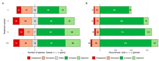
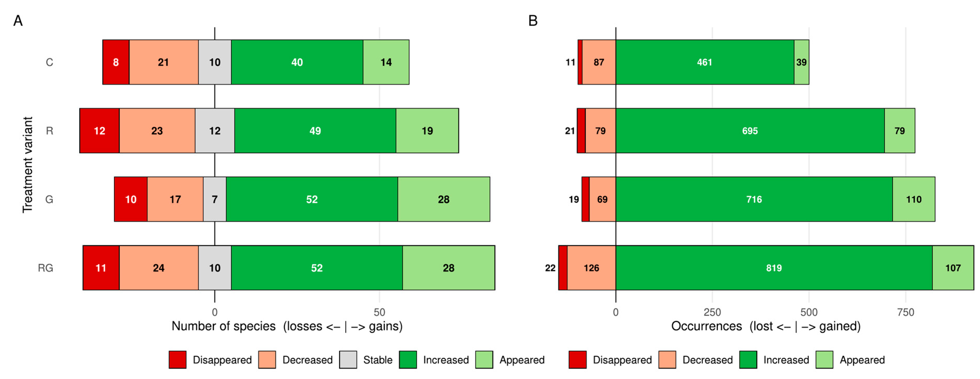
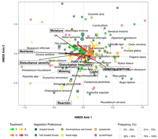
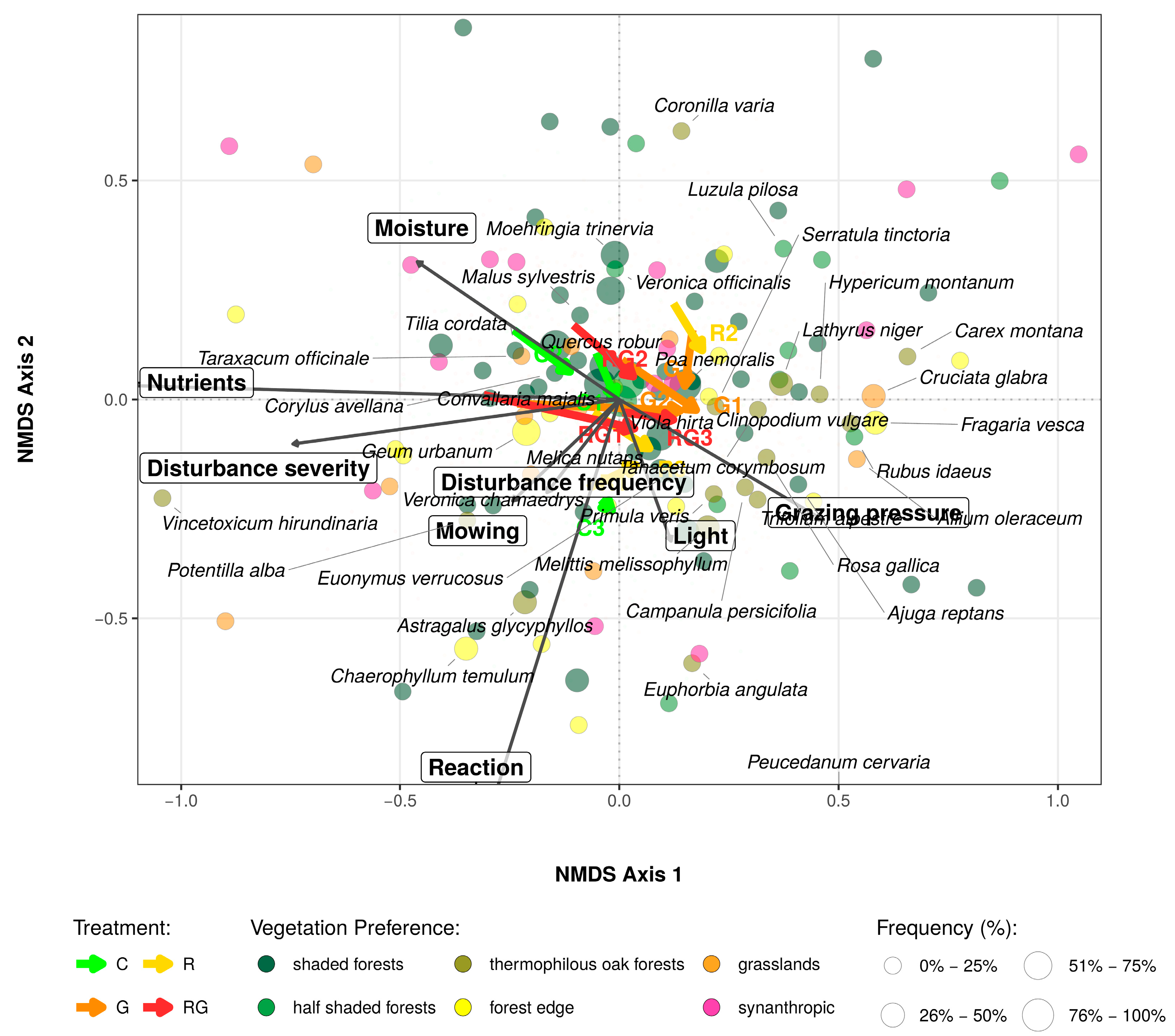
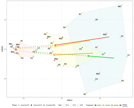
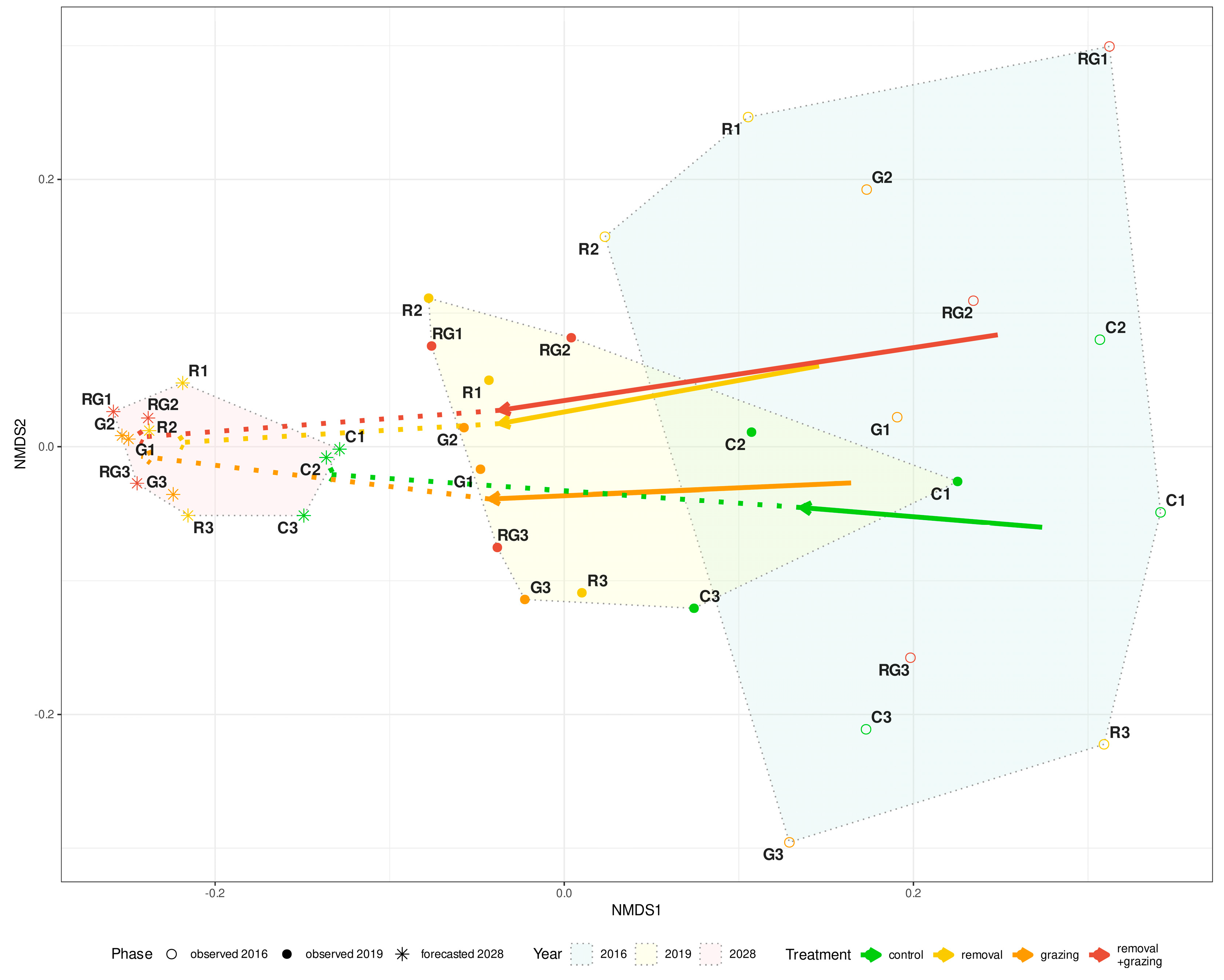
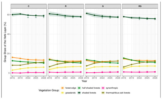
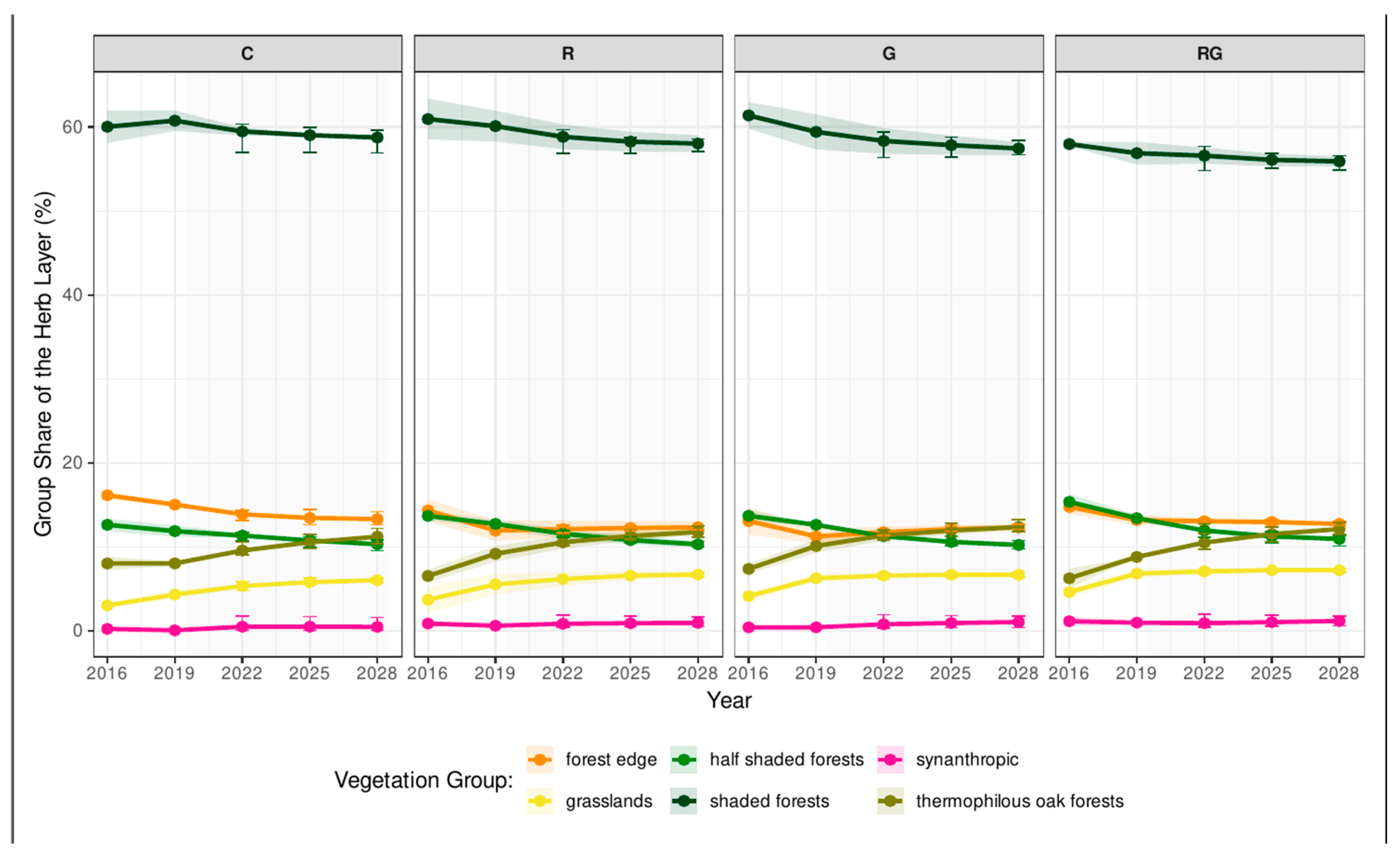
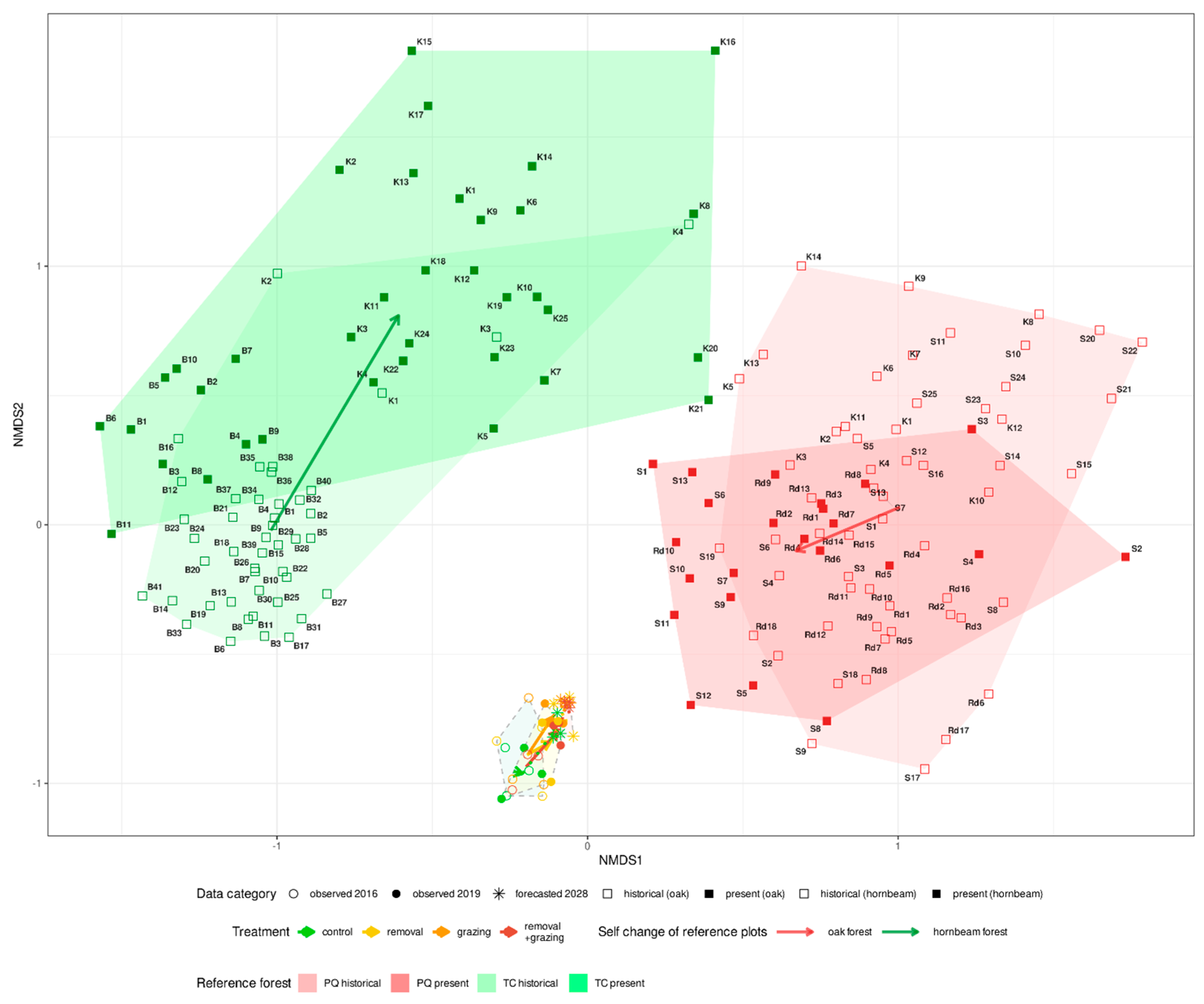
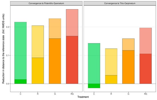
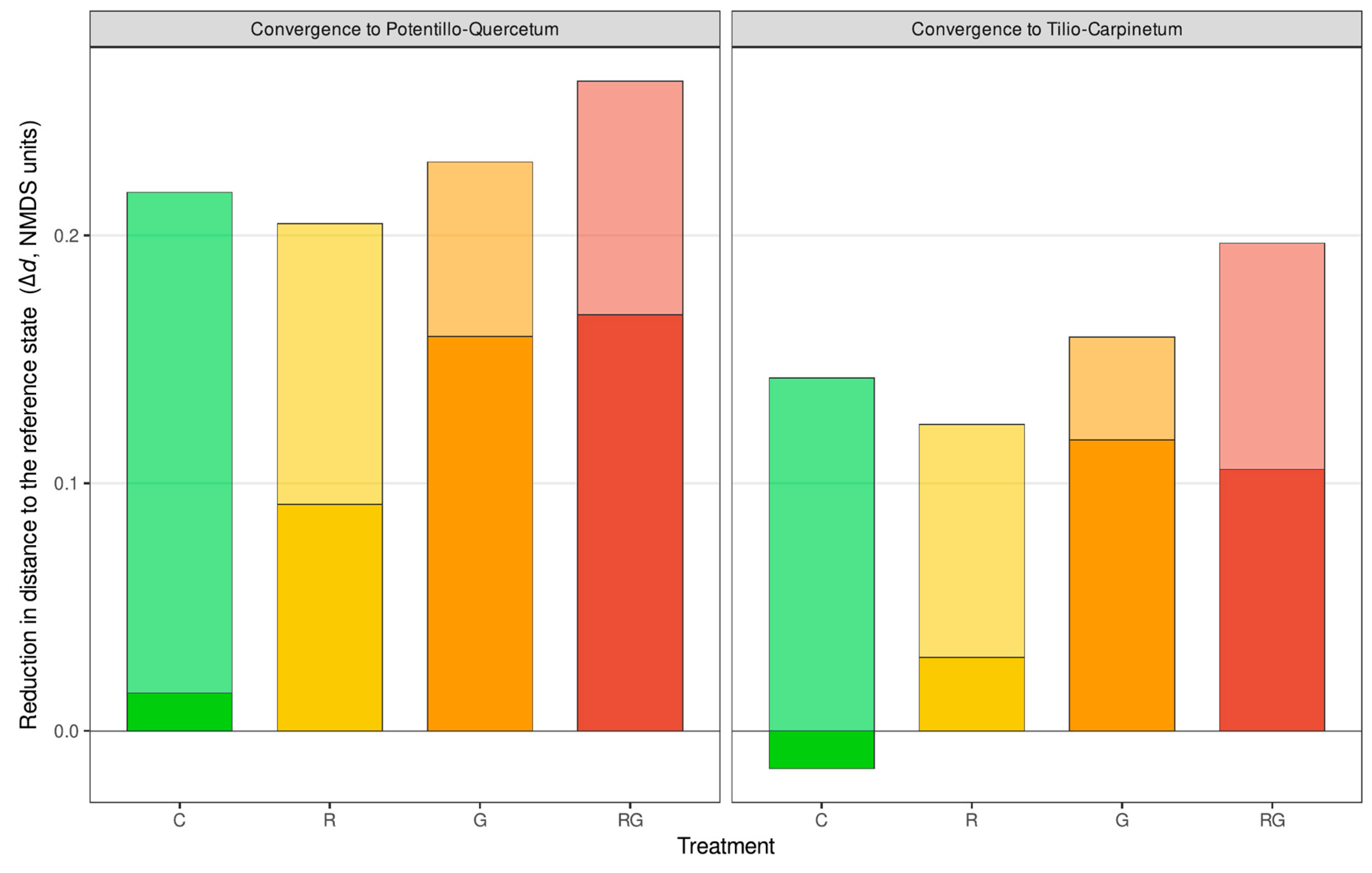

Disclaimer/Publisher’s Note: The statements, opinions and data contained in all publications are solely those of the individual author(s) and contributor(s) and not of MDPI and/or the editor(s). MDPI and/or the editor(s) disclaim responsibility for any injury to people or property resulting from any ideas, methods, instructions or products referred to in the content. |
© 2026 by the authors. Licensee MDPI, Basel, Switzerland. This article is an open access article distributed under the terms and conditions of the Creative Commons Attribution (CC BY) license.