


Abstract
Quantifying current topsoil organic matter (SOM) differences associated with cropland retirement is challenging because soil observations are spatially uneven and historical SOM maps are scarce. We integrated 10,262 measurements of 0–20 cm SOM collected in 2023 with remote sensing and environmental covariates and annual land-cover histories from 1999 to 2023 in western Shanxi, China. Random forest (RF), support vector regression, and multiple linear regression were compared using five-fold cross-validation. Ten bootstrap RF prediction runs were used to derive a mean SOM map and a pixel-wise standard deviation layer representing between-run prediction variability. RF achieved the best performance (R2 = 0.52; RMSE = 5.43 g kg−1; MAE = 3.41 g kg−1). Strict one-to-one matching showed that predicted SOM was 3.084 g kg−1 higher in converted croplands than in cropland reference areas. The mean difference was larger for forestland-covered converted croplands (4.960 g kg−1) than for grassland-covered converted croplands (3.019 g kg−1). Earlier conversion cohorts generally showed larger spatial contrasts. A complementary local comparison yielded a mean difference of 3.004 g kg−1 and revealed substantial spatial heterogeneity. These results represent current predicted spatial differences associated with reconstructed land-cover histories rather than directly measured temporal SOM gains or causal effects of the Grain-for-Green Program.
1. Introduction
Soil organic matter (SOM) is a fundamental component of soil quality, influencing nutrient supply, soil structure, water retention, and resistance to degradation [1]. Evidence linking soil organic carbon (SOC) with crop production further emphasizes the agricultural importance of maintaining organic matter, although responses depend on environmental and management conditions [2]. Maintaining and restoring soil carbon pools is also important for climate change mitigation and food security [3,4]. In topsoil, organic matter responds to plant inputs, cultivation disturbance, erosion, and restoration, making it relevant to assessments of land degradation and ecological recovery [5]. However, SOM commonly exhibits strong spatial heterogeneity over hilly landscapes, where topography, parent material, vegetation, climate, and management interact across short distances. Spatially explicit assessment therefore requires approaches that integrate soil observations with environmental information rather than relying only on point summaries [6,7].
The loess hilly region of western Shanxi lies on the eastern Loess Plateau, where dissected terrain, cultivation on sloping land, and severe erosion have shaped soil redistribution and land-cover change [8]. Since 1999, the Grain-for-Green Program (GGP), also known as the Conversion of Cropland to Forest Program, has promoted the conversion of sloping or marginal cropland to vegetation cover as part of a large-scale ecological restoration effort [9]. National assessments have documented improvements in soil retention and ecosystem carbon sequestration associated with restoration and conservation investments [10,11]. Satellite observations also demonstrate the importance of land management to greening in China [12]. However, greening does not necessarily imply equivalent improvements in every ecosystem service: assessments of the GGP have identified gains in vegetation condition alongside water-related trade-offs [13]. Soil carbon responses likewise vary with restoration age, vegetation type, and environmental setting [14,15], motivating a spatially explicit assessment of topsoil SOM in this heterogeneous region. Forest restoration is particularly relevant to soil carbon assessment because changes in canopy cover, litter inputs, root systems, erosion protection, and soil moisture can alter the quantity and spatial distribution of topsoil organic matter. However, the soil response of forestland established through Grain-for-Green may differ from that of grassland restoration, and regional evidence remains limited where historical soil carbon observations are unavailable.
Digital soil mapping provides a framework for predicting soil properties from their relationships with environmental covariates. The SCORPAN concept formalizes soil variation in terms of soil, climate, organisms, relief, parent material, age, and spatial position [6]. Reviews of SOC mapping identify vegetation, terrain, climate, and land use as important predictor groups, with their relative contributions varying among scales and landscapes [7]. Remote-sensing bands and indices provide information on surface reflectance, vegetation condition, and bare soil exposure that can complement terrain and climate data [16]. SoilGrids 2.0 illustrates the potential of combining soil observations with environmental covariates for spatial prediction and uncertainty characterization [17]. In Loess watersheds, field evidence of land-use and topographic influences on SOC distribution further supports using a landscape-based predictor framework [18]. Dense local observations can help adapt this framework to the pronounced heterogeneity of the western Shanxi hills.
Machine learning models are increasingly used in digital soil mapping to represent complex relationships between soil properties and environmental covariates [19,20]. Random forest (RF) combines multiple decision trees and provides measures of predictor importance [21]. Support vector regression (SVR) provides a kernel-based modeling framework [22], while multiple linear regression (MLR) offers an interpretable linear benchmark. Comparative work in digital soil mapping indicates that the suitability of RF, support vector regression, and MLR depends on the data, model configuration, and mapping objective rather than a universally superior algorithm [23]. Comparing these approaches using the same observations and validation design therefore provides an empirical basis for choosing the SOM mapping model, while keeping prediction performance distinct from ecological interpretation [20].
Long-term annual land-cover products make it possible to connect current SOM mapping with reconstructed land-use trajectories. The China Land Cover Dataset (CLCD) provides Landsat-derived annual information at 30 m resolution for monitoring land-cover dynamics in China [24,25]. The updated annual layers were obtained from the Zenodo data release [25]. In this study, annual maps for 1999–2023 were used to identify cropland-to-forestland, cropland-to-grassland, and cropland-to-shrubland transitions, while cropland histories were used to define cropland reference areas. Such trajectories add a temporal dimension to static SOM prediction, but they do not constitute repeated soil observations. The distinction between land-cover monitoring and measurement of soil carbon change is important when interpreting spatial comparisons as evidence of restoration-associated differences [26]. The 2023 SOM observations describe current soil conditions, whereas the 1999–2023 land-cover sequence describes land-use history.
Existing studies have established the usefulness of remote sensing, environmental covariates, and machine learning models for regional soil property mapping [16,20]. However, many assessments focus on producing a soil property map without reconstructing annual land-use histories, compare broad land-cover classes without explicit environmental matching, or lack sufficient field observations to evaluate spatial contrasts among restoration types. In addition, a higher soil property value in restored vegetation does not by itself demonstrate a temporal increase or a causal effect of restoration because historical soil observations are often unavailable. Previous studies often focus on mapping soil properties or comparing endpoint land-cover classes, whereas annual conversion trajectories and spatially matched comparisons are less commonly combined with dense laboratory observations for restoration assessment.
To address these limitations, this study integrates high-density 2023 topsoil SOM observations, annual 30 m land-cover histories from 1999 to 2023, and two complementary spatial comparison designs. Specifically, we (1) map current 0–20 cm topsoil SOM in the loess hilly region of western Shanxi using remote sensing and environmental covariates; (2) compare RF, SVR, and MLR models using the same observations and validation framework; and (3) identify cropland retirement trajectories and quantify current SOM differences associated with likely GGP-related conversion relative to cropland reference areas, with particular emphasis on contrasts between forestland and grassland restoration. The study therefore provides a field-supported, spatially explicit assessment of current SOM differences associated with reconstructed land-cover histories, rather than a direct measurement of temporal SOM gains or a causal evaluation of the GGP. The comparison therefore estimates current spatial contrasts among locations with different land-cover histories, rather than the amount of SOM gained by any particular cropland parcel after conversion.
The specific contribution of this study is centered on the integration of three elements. First, it uses a relatively dense set of verified field measurements collected in the same year to characterize current topsoil SOM across a heterogeneous hilly region. Second, it links the current SOM surface to annual 30 m land-cover trajectories rather than using only a single endpoint land-cover map. Third, it compares converted areas with environmental cropland reference areas using both strict one-to-one matching and a complementary local spatial analysis. These comparisons are designed to describe current spatial contrasts and restoration monitoring priorities.
2. Materials and Methods
2.1. Study Area
The study area is located in the loess hilly region of western Shanxi Province, China, along the eastern margin of the Loess Plateau (Figure 1). It covers approximately 35,200 km2 and ranges in elevation from about 380 to 2785 m above sea level. The landscape is characterized by deeply dissected loess hills, dense gully networks, pronounced local relief, and extensive areas of sloping croplands. The regional climate ranges from semi-arid to semi-humid and is influenced by the East Asian monsoon. The mean annual temperature ranges from approximately −1.2 to 13.7 °C, while mean annual precipitation varies from 355 to 627 mm. Precipitation is concentrated during the growing season, promoting runoff generation and soil erosion on hillslopes. The combined effects of erodible loess, highly fragmented terrain, seasonally concentrated rainfall, and long-term agricultural activities make the region highly susceptible to soil erosion and land degradation.
Figure 1.
Location of the study area in western Shanxi, China, and spatial distribution of soil-sampling sites.
The study area has experienced substantial land-cover changes under ecological restoration policies, particularly the Grain-for-Green Program (GGP), which was initiated in 1999. The coexistence of retired croplands, continuously cultivated croplands, complex terrain, and heterogeneous soil conditions provides a suitable setting for mapping the current spatial distribution of soil organic matter (SOM) in the 0–20 cm soil layer and assessing GGP-associated SOM differences under comparable environmental conditions.
2.2. Soil Sampling and SOM Measurement
In 2023, a total of 10,262 topsoil samples were collected from the 0–20 cm layer throughout the study area. Sampling followed a grid-based spatial design, with increased sampling density in areas showing strong terrain and elevation variability and in areas representing different distributions of cropland, grassland, forestland, and shrubland. Each sampling location was represented by a composite sample formed by thoroughly mixing soil collected from three nearby subsampling points. The final dataset comprised 6874 cropland, 2212 grassland, 965 forestland, and 211 shrubland observations. Surface litter and loose surface fragments were removed before sampling. The sampling design was intended to improve representation of the main terrain, land-cover, and environmental conditions in the region; it was therefore a spatially designed and environmentally informed grid survey with targeted densification, rather than a simple random sample of the regional soil population. The resulting measurements represent mineral soil SOM in the standardized 0–20 cm layer and do not include the litter layer or forest floor organic material. The target sampling depth was standardized as 0–20 cm across the study area, and nearly all sampling locations met the full 20 cm requirement. At a very small number of locations where the available soil layer was shallower because of severe erosion, shallow soil development, or field conditions, sampling was conducted to the maximum available soil depth. Exposed parent material was not excavated or intentionally included in the soil samples.
SOM was determined by oxidizing soil organic carbon with an excess potassium dichromate–sulfuric acid solution under externally heated conditions, followed by titration of the residual potassium dichromate with a standardized ferrous sulfate solution. The amount of oxidized organic carbon was calculated from the potassium dichromate consumed using the applicable oxidation correction factor. SOM was then calculated as SOC × 1.724, where 1.724 is the reciprocal of the assumed mean carbon fraction of soil organic matter (58%). Quality control consisted of checking the measured values against laboratory records and data entry files, together with verification against land-cover, ecological, and soil classification information. No experimental or data-entry errors were identified, and the reported results are based on the verified SOM dataset.
2.3. Identification of GGP-Related and Cropland Reference Areas
GGP-associated land-cover transitions and cropland reference areas were identified using annual 30 m CLCD land-cover maps for 1999–2023 [24,25]. Because official parcel-level boundaries for GGP projects were unavailable, cropland-to-forestland, cropland-to-shrubland, and cropland-to-grassland transitions were treated as land-cover-based proxies for likely GGP-related conversion given the policy context in which cropland generally cannot be abandoned or converted without authorization. The conversion categories were identified from the multi-year annual land-cover trajectory rather than from a single-year classification. This trajectory-based approach reduces reliance on any one potentially ambiguous annual label, although temporary fallow conditions, spontaneous herbaceous cover, phenological differences, and mixed pixels may still cause cropland/grassland confusion.
Annual event-based transitions between consecutive years were quantified to characterize conversion and recultivation dynamics. A conversion event was recorded when cropland changed to forestland, shrubland, or grassland, whereas a recultivation event was recorded when any of these vegetation classes changed back to cropland. These transitions describe observed land-cover trajectories and do not by themselves verify the administrative implementation of a GGP project. Accordingly, a mapped cropland-to-grassland transition is interpreted as a land-cover trajectory and a GGP-related conversion proxy, not as independently verified evidence of a particular restoration project. The reported cumulative areas of retirement and return-to-agriculture events represent gross year-to-year transition extents, rather than unique areas of confirmed persistent conversion. A pixel that changes class repeatedly may contribute to more than one annual event, and successive reversals may reflect either actual land-use dynamics or short-term classification instability.
The persistence-threshold sensitivity analysis was conducted using two-, three-, and five-year endpoint persistence criteria. These criteria changed the eligible conversion area, but the analysis was used to assess area stability and was not used to claim causal robustness. The one-year endpoint criterion was retained as the baseline description, whereas the 2-, 3-, and 5-year criteria were used to quantify the stability of the endpoint conversion area and to exclude short-lived transitions from progressively stricter assessments.
The local pixel-based comparison used a separate endpoint definition: pixels that were cropland in 1999 and forestland, shrubland, or grassland in 2023. Each pixel was counted once, and its vegetation type was assigned from the 2023 map. Pixels classified as cropland in 1999 and continuously classified as cropland from 2019 through 2023 were retained as local cropland reference areas. Because complete annual management records were unavailable, these reference pixels cannot be guaranteed to have remained continuously cultivated or to represent a perfect counterfactual. These cropland reference pixels should not be interpreted as a strictly continuous-agriculture reference group: the endpoint criteria do not exclude temporary retirement followed by recultivation during the intervening years.
2.4. Environmental Variables
The candidate environmental inventory comprised 23 variables describing climate, vegetation, soil background, terrain, human activity, and land-surface conditions (Table 1). Climate variables described mean annual precipitation (MAP), mean annual temperature (MAT), and potential evapotranspiration (PET); vegetation variables comprised annual Normalized Difference Vegetation Index (NDVI). Soil genus (TS) and parent material (PM) represented soil-forming background, while elevation and DEM-derived terrain and hydrological attributes characterized relief and landscape position. Land cover (LC) information and remote sensing variables, including normalized difference moisture index (NDMI), temperature vegetation dryness index (TVDI), land surface temperature (LST), and near-infrared reflectance (NIR) completed the inventory. The environmental raster stack was aligned with the 30 m analysis grid and extracted at soil-sampling locations.
Table 1.
Candidate environmental variables, source resolutions, and data sources.
2.5. Variable Selection
Variable selection focused on reducing multicollinearity among numeric environmental predictors. Variance inflation factors (VIFs) were used for screening, with a retention criterion of VIF < 10. Sixteen numeric predictors were retained: NDVI, slope, NDMI, terrain ruggedness index (TRI), MAT, elevation (DEM), channel network distance (CND), valley depth (VD), topographic wetness index (TWI), PET, MAP, plan curvature (PLC), TVDI, convergence index (CI), profile curvature (PRC), and channel network base level (CNBL). Their VIF values ranged from 1.13 to 8.67, all below the retention threshold (Figure 2).
Figure 2.
VIF values for the 16 retained numeric predictors, ranked from highest to lowest. The dashed line marks the retention threshold of 10. All values were below this threshold. Abbreviations: PET—potential evapotranspiration; DEM—digital elevation model; CND—channel network distance; NDMI—normalized difference moisture index; VD—valley depth; NDVI—Normalized Difference Vegetation Index; MAT—mean annual temperature; TRI—terrain ruggedness index; TWI—topographic wetness index; TVDI—temperature vegetation dryness index; MAP—precipitation; PLC—plan curvature; CI—convergence index; PRC—profile curvature; CNBL—channel network base level.
LC, PM, and TS were retained as categorical predictors representing land-cover and soil-forming conditions. Soil genus denotes the third-level soil category in the classification used for this dataset. These variables were treated as nominal categories rather than continuous quantities; the numeric VIF threshold was not applied directly to their class codes. The final set therefore comprised 19 predictors (16 numeric and three categorical variables). The same predictor set was used for RF, SVR, and MLR to ensure a fair comparison.
2.6. Modeling Approaches
Three regression approaches were compared: random forest (RF), support vector regression (SVR), and multiple linear regression (MLR). All modeling procedures were implemented in Python 3.15.0 using scikit-learn, NumPy, pandas, and Rasterio. RF was implemented using RandomForestRegressor with 500 trees, bootstrap sampling, and a minimum terminal-node sample size of three. Predictor importance was assessed using the default impurity-based importance measure, and the values were normalized so that their sum equaled 100%. The RF predictor-importance values used the default impurity-based importance measure. Values were normalized so that the importance values of all predictors summed to 100%; they therefore represent relative predictive use within this fitted model rather than independent or causal contributions. In this measure, the contribution of a predictor is accumulated from the impurity reductions associated with its splits across the fitted trees.
2.7. Model Validation and Mapping
Model validation used five-fold cross-validation, with four folds used for training and the remaining fold used for validation. Validation performance was summarized using R2, RMSE, and MAE across the validation predictions. Separately, 10 bootstrap RF models were fitted for ensemble mapping. Each bootstrap model was used to predict the full 30 m study area grid. The final SOM map was calculated as the pixel-wise mean of the 10 bootstrap prediction rasters, and the pixel-wise standard deviation was calculated as an empirical measure of between-run ensemble variability.
2.8. Statistical Analysis of GGP Effects
The primary statistical assessment was conducted on the RF-predicted SOM raster. Candidate GGP-related and cropland reference locations were selected by spatial subsampling on a grid with a 10-pixel interval (300 m), followed by valid data screening. Each GGP candidate was matched one-to-one without replacement to a cropland reference candidate with the same soil genus and aspect class, an elevation difference no greater than 50 m, a slope difference no greater than 3°, and a geographic distance no greater than 10 km. Slopes below 2° formed a nearly flat class; other slopes were grouped by aspect into north (315–360° or 0–45°), east (45–135°), south (135–225°), and west (225–315°), using left-inclusive and right-exclusive intervals. Matching proceeded sequentially through the retained GGP candidate list; cropland reference locations already used in a pair were unavailable for subsequent matches. GGP candidates without an eligible unused cropland reference candidate were excluded.
When multiple eligible cropland reference pixels remained, the cropland-reference pixel with the lowest composite score was selected. The score summed geographic distance divided by 10 km, absolute elevation difference divided by 50 m, and absolute slope difference divided by 3°. Two additional terms were included: 0.3 times the absolute temperature difference divided by 2 °C and 0.3 times the absolute precipitation difference divided by 100 mm; each climate ratio was capped at 5 before weighting. These climate terms ranked eligible cropland reference candidates but did not impose additional exclusion thresholds. SOM and vegetation indices were not used in the matching score.
Matching quality was assessed using standardized mean differences (SMDs) for elevation, slope, temperature, and precipitation, with absolute SMDs below 0.1 indicating acceptable balance [27]. Paired SOM differences were calculated as follows:
where denotes a matched GGP-related–cropland-reference pair; and are the predicted topsoil (0–20 cm) SOM concentrations in the retired-cropland pixel (GGP) and its matched cropland reference pixel, respectively; and is their paired SOM difference. All three SOM quantities are expressed in g kg−1. Positive and negative differences indicate higher and lower predicted SOM in GGP pixels relative to cropland reference pixels, respectively.
Relative differences were calculated for each pair as
where is the relative SOM difference for pair , expressed as a percentage. Paired SOM differences and relative differences were averaged separately within each analysis group. These quantities represent spatial contrasts in 2023, not directly observed before-and-after changes.
Prediction variability in the final SOM surface was characterized using the pixel-wise standard deviation of the 10 bootstrap RF prediction rasters. Among valid pixels, the mean standard deviation was 0.634 g kg−1, the median was 0.510 g kg−1, the standard deviation was 0.491 g kg−1, and the 1st–95th percentile range was 0.093–1.616 g kg−1. The maximum value was 7.093 g kg−1.
The bootstrap ensemble captures variability among the retained bootstrap model runs; it does not include all sources of measurement error, sampling uncertainty, land-cover classification error, or extrapolation error.
The matching analysis therefore reports spatial contrasts conditional on the mean SOM prediction surface and the selected reference pixels. These contrasts do not incorporate all sources of model-fitting, land-cover classification, sampling, or matching-selection uncertainty.
A complementary pixel-level spatial contrast was calculated for pixels that were cropland in 1999 and forestland, shrubland, or grassland in 2023. Pixels classified as cropland in 1999 and continuously classified as cropland from 2019 through 2023 served as local cropland reference areas. This analysis is presented as a descriptive spatial sensitivity analysis, whereas the strict one-to-one matching analysis is the primary comparison.
3. Results
3.1. Prediction Accuracy and Spatial Distribution of Topsoil SOM
The three regression models differed substantially in their ability to predict 0–20 cm topsoil SOM (Table 2). Random forest (RF) achieved the best predictive performance, with an R2 of 0.52, an RMSE of 5.43 g kg−1, and an MAE of 3.41 g kg−1. The support vector regression (SVR) model showed moderate performance, with an R2 of 0.39, an RMSE of 6.12 g kg−1, and an MAE of 3.88 g kg−1. Multiple linear regression (MLR) performed weakest among the three models, with an R2 of 0.32, an RMSE of 6.46 g kg−1, and an MAE of 5.59 g kg−1. These results indicate that RF better captured the nonlinear relationships between SOM and remote sensing, topographic, climatic, and land-cover covariates. Therefore, RF was selected as the final model for spatial prediction of topsoil SOM.
Table 2.
Validation performance of the three SOM prediction models.
The final RF-derived 2023 SOM map revealed substantial spatial heterogeneity across the study region (Figure 3). SOM ranged from 1.75 to 105.88 g kg−1, with an area-weighted mean of 15.85 g kg−1, a median of 13.13 g kg−1, and a standard deviation of 9.34 g kg−1. The highest measured SOM value was 141.23 g kg−1. All high-value samples were checked against their recorded land-cover types, ecological settings, and soil classifications, and the laboratory records and data entry files were verified. No experimental or data-entry errors were identified, so these values were retained as valid observations. The highest predicted values were concentrated mainly in forestland areas, within environmental settings represented by the field dataset. Such values are ecologically plausible in locations with greater organic inputs and reduced cultivation disturbance, but they remain model predictions rather than direct measurements.
Figure 3.
Predicted spatial distribution of 0–20 cm soil organic matter (SOM) in 2023, derived from the final random forest model.
The corresponding RF prediction variability layer showed generally low to moderate between-run variability across most valid pixels (mean 0.634 g kg−1; median 0.510 g kg−1), with higher values occurring in localized areas (Figure 4). This layer provides spatial context for interpreting the regional SOM surface and the group-level comparisons.
Figure 4.
Spatial distribution of RF prediction variability for 0–20 cm topsoil SOM. Values show the pixel-wise standard deviation among 10 bootstrap RF prediction runs; the color scale is truncated at the 1st and 95th percentiles for visualization.
The land-cover-based statistics further showed that mean predicted SOM was 10.32 g kg−1 in cropland, with a median of 10.06 g kg−1. Grassland had a mean of 14.23 g kg−1 and a median of 13.40 g kg−1; forestland had a mean of 27.77 g kg−1 and a median of 26.63 g kg−1; and shrubland had a mean of 25.52 g kg−1 and a median of 24.14 g kg−1 (Table 3).
Table 3.
Summary statistics of measured topsoil SOM by land-cover class.
The field observations showed strong right skewness in all land-cover classes. Cropland samples had a mean SOM of 9.82 g kg−1, median of 8.42 g kg−1, and standard deviation of 4.31 g kg−1 (skewness 3.21; kurtosis 40.24; n = 6874). The corresponding values were 14.12, 9.42, and 13.28 g kg−1 for grassland (skewness 2.76; kurtosis 15.43; n = 2212), 24.13, 14.70, and 20.93 g kg−1 for forestland (skewness 2.14; kurtosis 8.78; n = 965), and 18.13, 11.69, and 16.24 g kg−1 for shrubland (skewness 2.46; kurtosis 10.92; n = 211). Sample-based and map-based means summarize different spatial and land-cover distributions and should not be expected to be identical.
The observed and RF-mapped class means showed the same broad ordering: cropland < grassland < shrubland < forestland. The observed means were 9.82, 14.12, 18.13, and 24.13 g kg−1 for cropland, grassland, shrubland, and forestland, respectively, whereas the corresponding RF-mapped means were 10.32, 14.23, 25.52, and 27.77 g kg−1. This agreement indicates that the model preserved the main differences among the land-cover and environmental groups represented in the field data. The two sets of means were not expected to be identical because the field statistics summarize the sampled locations, whereas the mapped statistics summarize all valid pixels within each land-cover class across the study region. The comparison therefore assesses broad class-level consistency rather than exact distributional equivalence or prediction accuracy at every sampling location. Because the field observations were not collected under an environmentally balanced experimental design, this agreement should be interpreted as an exploratory consistency check rather than as evidence that all environmental differences among land-cover classes have been statistically removed. The comparison nevertheless indicates that the main class-level ordering is also present in the laboratory data, despite land cover being included as a model predictor.
The available sample-level summaries do not include a paired comparison between observed SOM and the corresponding RF predictions at every sampling location. We therefore use the observed land-cover summaries to characterize the field data and do not claim a direct distributional equivalence between the measured samples and the regional prediction raster. The land-cover classes were not equally represented: cropland and grassland contributed most observations, whereas forestland and shrubland were less represented. The highest measured SOM concentration was 141.23 g kg−1. These high-value observations were checked against their recorded land-cover types, ecological settings, and soil classifications, and no experimental or data entry errors were identified; they were therefore retained as valid field observations.
As an exploratory field data check, the coordinates of the 10,262 measured samples were overlaid with the map-defined GGP-related conversion proxies and cropland-reference mask. Among all measured samples, 952 were located within the GGP-related conversion proxies and 2176 within the cropland-reference areas. The mean measured SOM concentration was 14.96 g kg−1 in the GGP-related samples and 10.68 g kg−1 in the cropland-reference samples, corresponding to a descriptive difference of 4.28 g kg−1. The direction of this field-observed difference was consistent with the RF-based matched contrast of 3.084 g kg−1. Because the field samples were not collected as a randomized GGP-related–cropland-reference experiment and the two comparisons use different spatial supports, this agreement is interpreted as exploratory consistency rather than causal validation.
Overall, RF provided the most reliable prediction among the three tested approaches and generated a continuous 2023 SOM map suitable for subsequent GGP-related–cropland-reference comparison. The SOM map not only characterized the current spatial pattern of topsoil SOM in the study region, but also provided the raster basis for assessing SOM differences between retired croplands and cropland reference areas.
3.2. Relative Importance of Environmental Predictors
The RF feature importance analysis showed contributions from vegetation, terrain, moisture, climate, land cover, and soil-forming background across the 19 predictors (Figure 5). Importance was calculated using the default impurity-based RF measure and normalized to a total of 100%. Because correlated predictors can share or redistribute impurity-based importance, these percentages describe relative predictive use rather than independent causal effects.
Figure 5.
Relative importance of the 19 environmental predictors in the final random forest SOM model. Horizontal bars show relative predictor importance percentages, which sum to 100%. Predictors are ordered from highest to lowest importance. Abbreviations: PET—potential evapotranspiration; DEM—digital elevation model; CND—channel network distance; NDMI—Normalized difference moisture index; VD—valley depth; NDVI—Normalized Difference Vegetation Index; MAT—mean annual temperature; TRI—terrain ruggedness index; TWI—topographic wetness index; TVDI—temperature vegetation dryness index; MAP—precipitation; PLC—plan curvature; CI—convergence index; PRC—profile curvature; CNBL—channel network base level; PM—parent material; LC—land cover; TS denotes soil genus.
Among the remote sensing indices, NDVI and NDMI ranked first and third, respectively, whereas TVDI contributed 3.92%. These indices provided information on vegetation condition and surface-moisture-related variability that contributed to regional SOM prediction. These percentages should not be interpreted as the proportion of SOM formation or recovery attributable to each predictor. Because several predictors may share environmental information, the values are not an independent variance decomposition and do not indicate the direction of any relationship. The reported percentages are therefore conditional on the fitted predictor set and RF configuration.
Terrain predictors were also prominent. Slope, TRI, and DEM contributed 8.01%, 6.91%, and 5.67%, respectively. Plan curvature (4.10%), convergence index (3.62%), and profile curvature (3.47%) provided additional information on terrain configuration. The contributions of these variables show that SOM prediction used multiple aspects of relief rather than elevation or slope alone.
Hydrological and landscape-position attributes contributed throughout the ranking. Channel network distance accounted for 5.41%, valley depth for 4.82%, topographic wetness index for 4.79%, and channel network base level for 3.41%. These variables complemented the terrain predictors by representing spatial differences in drainage and landscape position.
Among the climatic predictors, mean annual temperature had the greatest importance (6.27%), followed by PET (4.49%) and precipitation (4.41%). Thus, both thermal conditions and water-related climatic variables contributed to the RF predictions.
The categorical predictors made distinct contributions. Land cover (5.36%) ranked above soil genus (5.12%), while parent material ranked last among the 19 predictors at 2.81%. Land cover represented differences among current land-cover classes, whereas soil genus and parent material provided complementary soil-background information. Soil genus was also used as an exact-matching condition in the GGP-related–cropland-reference comparison.
Overall, the importance distribution indicates that regional SOM prediction drew on multiple environmental dimensions, with vegetation indices and terrain attributes occupying several leading positions and land cover contributing additional categorical information. These percentages describe relative importance within the fitted RF model. Predictor importance describes the fitted model and does not quantify a causal effect of any individual environmental variable.
3.3. CLCD-Derived Retired Croplands and Land-Cover Dynamics
Annual land-cover trajectories were summarized using two distinct area measures: cumulative retirement and recultivation events, which may count a location repeatedly, and endpoint cropland-to-vegetation conversion, which counts each eligible 1999-cropland pixel once according to its 2023 cover. The first detectable transition year was 2000 because 1999 was the baseline.
Under the annual event-based definition, the cumulative area of cropland-to-forestland, cropland-to-shrubland, and cropland-to-grassland transition events from 2000 to 2023 was 8734.59 km2 (Figure 6). During the same period, the cumulative area of recultivation events, defined as forestland, shrubland, or grassland changing back to cropland, was 6378.30 km2. The annual retired-cropland event area showed substantial interannual variability rather than a monotonic trend. The largest annual retirement event areas occurred in 2017, 2004, 2010, 2009, and 2006, with corresponding areas of 535.09, 521.59, 517.07, 509.67, and 496.47 km2, respectively. Recultivation events were also evident in several years, indicating temporally dynamic land-cover transitions in the study area.
Figure 6.
Cropland retirement and recultivation dynamics during 2000–2023. (a) Cumulative retirement and recultivation event areas; (b–d) annual cropland retirement event areas with forestland, shrubland, and grassland as the immediate destination classes, respectively. Every year is shown. Panels (b–d) use different vertical axis scales. Repeated changes at one location may contribute multiple events; 1999 is the baseline year.
The annual retirement events were dominated by transitions from cropland to grassland. From 2000 to 2023, cropland-to-grassland events accumulated to 8638.54 km2, whereas cropland-to-forestland and cropland-to-shrubland events accounted for only 94.26 and 1.79 km2, respectively.
The endpoint cropland-to-vegetation conversion area, comprising pixels classified as cropland in 1999 and forestland, shrubland, or grassland in 2023, was 4569.75 km2. Grassland accounted for 4381.61 km2 (95.88%), forestland for 186.44 km2 (4.08%), and shrubland for 1.69 km2 (0.04%). These final-cover categories define the spatial extent of the local pixel-based SOM comparison. They differ from immediate transition destinations in the annual event statistics because a retired pixel may subsequently change between vegetation cover classes.
A persistence threshold sensitivity analysis was also conducted using the annual land-cover rasters. Under the one-year endpoint criterion, the converted area was 4569.75 km2. Requiring the endpoint vegetation class to persist for at least two, three, or five consecutive years reduced the corresponding converted areas to 4410.80, 4138.16, and 3968.73 km2, respectively. The area remained dominated by grassland: 4228.74, 3968.72, and 3819.44 km2 under the 2-, 3-, and 5-year criteria, respectively. Forestland areas were 180.77, 168.52, and 148.60 km2, and shrubland areas were 1.29, 0.92, and 0.69 km2. These results indicate that the broad spatial extent of the conversion domain is robust to stricter endpoint-persistence criteria, although the eligible area decreases as the persistence requirement becomes more stringent.
A strict one-to-one matching sensitivity analysis was conducted using the same candidate-grid spacing, covariate restrictions, search radius, and matching procedure, while changing only the endpoint persistence requirement. The resulting matched-pair counts were 18,430, 18,285, and 18,032 for the 2-, 3-, and 5-year criteria, respectively. The overall mean paired SOM differences were 3.048, 3.052, and 3.127 g kg−1, respectively. Forestland contrasts were 4.819, 4.662, and 4.869 g kg−1, whereas grassland contrasts were 2.987, 2.994, and 3.065 g kg−1. These results were similar to the primary estimate and remained positive under all three persistence criteria.
Within the endpoint-conversion domain, 1279.55 km2 was assigned to the 2000–2005 retirement cohort, equivalent to an annualized area of 213.26 km2 yr−1 (Table 4). The corresponding cohort areas were 955.12 km2 for 2006–2010, 983.70 km2 for 2011–2015, and 1351.38 km2 for 2016–2023, with annualized areas of 191.02, 196.74, and 168.92 km2 yr−1, respectively. Annualized cohort area was greatest in the earliest stage and lowest in 2016–2023. These values describe the retirement year composition of the area retained in 2023, rather than annual net changes in the total cropland inventory.
Table 4.
Endpoint cropland-to-vegetation conversion areas by retirement cohort and their annualized areas.
The transition-path analysis further showed that among pixels classified as cropland in 1999 and forestland in 2023, which covered 186.44 km2 in total, 137.72 km2 had been classified as grassland at least once before 2023, accounting for 73.87% of the final cropland-to-forestland area. This indicates that some pixels ending as forestland may have undergone a transitional cropland-–rassland–forestland pathway.
3.4. GGP-Associated Differences in Predicted Topsoil SOM
After spatial subsampling and valid data screening, 24,998 candidate converted pixels and 68,925 cropland reference candidates were available for strict matching. The environmental and distance constraints yielded 18,043 matched pairs, representing 72.18% of the converted candidates (Figure 7). The matched estimate therefore describes a spatial contrast between likely conversion areas and cropland reference areas under the stated matching criteria.
Figure 7.
Covariate balance before and after strict GGP-related–cropland-reference matching. Points show standardized mean differences for elevation, slope, temperature, and precipitation. Dashed vertical lines mark −0.1 and 0.1; values closer to zero indicate better balance.
Overall, converted croplands had higher mean predicted SOM concentrations than their environmentally matched cropland reference areas (Figure 8). Mean SOM was 12.598 g kg−1 for converted pixels and 9.513 g kg−1 for cropland reference pixels, yielding a mean paired difference of 3.084 g kg−1 and a median difference of 2.940 g kg−1. The average of the pair-specific relative differences was 37.58%, and 78.81% of matched pairs had SOM_converted > SOM_reference. These are spatial contrasts conditional on the mean SOM prediction surface and should not be interpreted as causal effects or direct temporal changes.
Figure 8.
Predicted topsoil SOM distributions in GGP-related conversion pixels and matched cropland reference areas, overall and by 2023 vegetation cover type. Boxes show interquartile ranges, horizontal lines show medians, whiskers show the 5th–95th percentiles, and dots show means. The overall group includes three shrubland pairs, which are not shown separately.
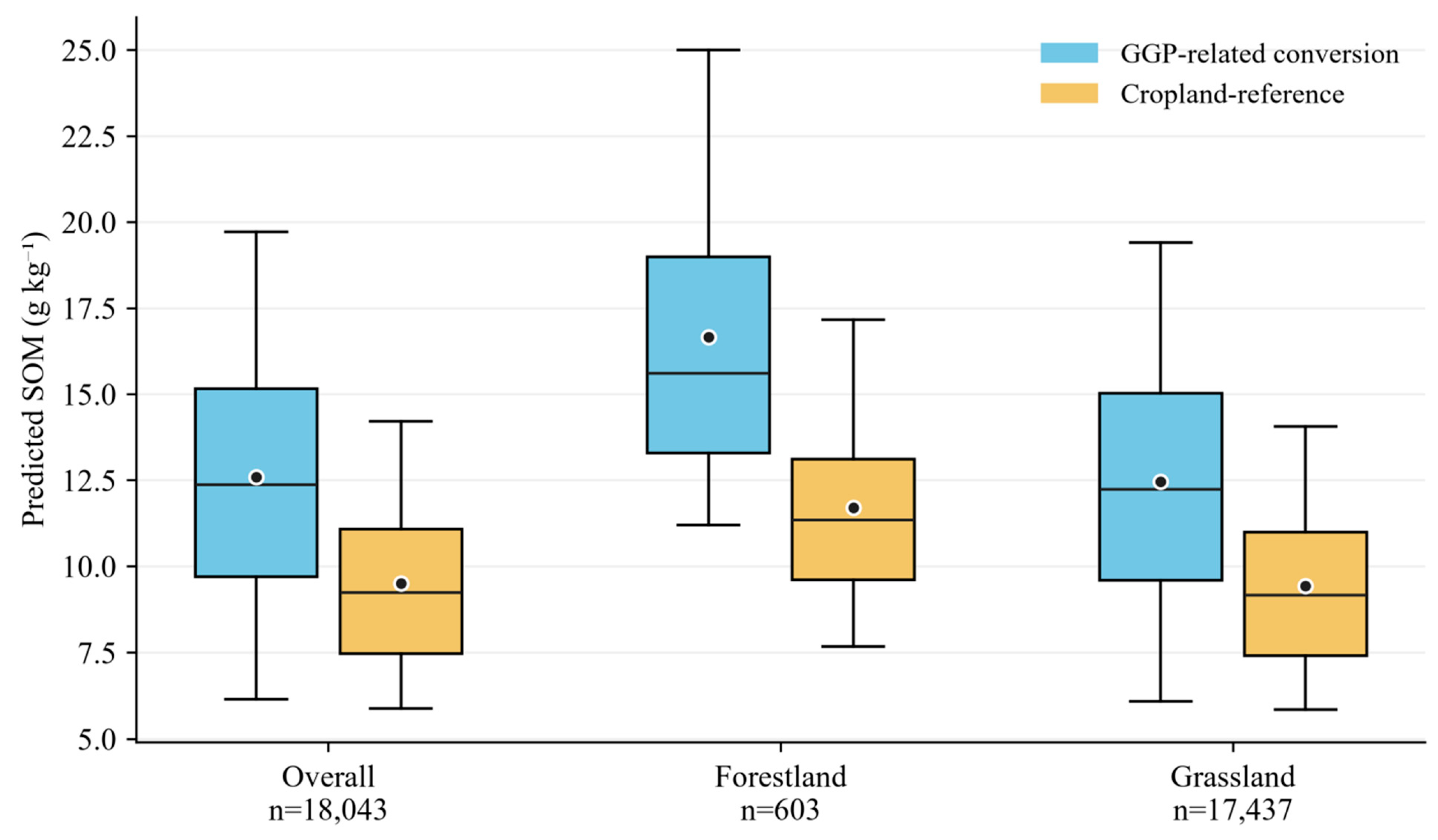
The magnitude of the SOM difference varied between post-conversion vegetation cover types (Figure 9). Forestland-covered converted croplands had a mean SOM of 16.668 g kg−1, compared with 11.708 g kg−1 in their reference croplands, corresponding to a mean difference of 4.960 g kg−1 (n = 603). Grassland-covered converted croplands accounted for most matched pairs (n = 17,437). Their mean SOM was 12.455 g kg−1, compared with 9.437 g kg−1 in reference croplands, yielding a mean difference of 3.019 g kg−1. Although the mean concentration difference was smaller for grassland than for forestland, grassland dominated the matched sample and converted cropland area. The three shrubland pairs were included in the overall estimate but were not interpreted inferentially.
Figure 9.
Mean paired SOM differences between GGP-related conversion pixels and cropland reference pixels, overall and by vegetation cover type. Points show means; uncertainty intervals should be interpreted as descriptive intervals conditional on the mean RF prediction surface and the matched sample.
The retirement-year analysis showed that earlier retirement cohorts had larger SOM differences in 2023 (Figure 10). Mean paired differences were 3.631 g kg−1 for 2000–2005, 3.024 g kg−1 for 2006–2010, 2.795 g kg−1 for 2011–2015, and 2.698 g kg−1 for 2016–2019 (Table 5). The largest annual cohort mean occurred in 2002 (3.935 g kg−1), although annual means did not decline monotonically. The stability requirement for vegetation cover during 2019–2023 excluded retirement years after 2019. Figure 9 therefore compares different retirement cohorts at a single observation time in 2023.
Figure 10.
Paired SOM differences by conversion cohort. Points show cohort means in 2023. The line connects cohort summaries. The results represent current spatial contrasts among conversion cohorts rather than directly measured temporal changes.
Table 5.
Predicted SOM contrasts from the strict matched-pair analysis.
Taken together, Figure 8 and Figure 9 show positive group-average SOM differences relative to cropland reference areas, with heterogeneity among vegetation cover types and conversion cohorts. Forestland-covered converted croplands had larger mean differences than grassland-covered converted croplands, while the larger spatial extent of grassland conversion means that grassland dominates the regional comparison. These patterns should be interpreted as associations in current predicted SOM, not as verified causal effects of GGP implementation.
3.5. Spatial Pattern of GGP-Associated SOM Differences
To characterize spatial heterogeneity, a pixel-level SOM contrast map was generated for pixels classified as cropland in 1999 and forestland, grassland, or shrubland in 2023. Local cropland-reference pixels were defined as pixels classified as cropland in 1999 and continuously classified as cropland from 2019 through 2023. Each contrast was calculated using the square neighborhood and minimum valid cropland reference count specified in Section 2.8:
where i identifies a retired-cropland pixel, j identifies a local cropland-reference pixel, ni is the number of valid local cropland-reference pixels, and SOMijref is the predicted SOM concentration of the j-th reference pixel associated with retired pixel i. The summation runs over all valid local cropland-reference pixels, so the subtracted term is their arithmetic mean SOM. GGP denotes retired cropland and cropland-reference denotes the reference areas. SOM concentrations and their differences are expressed in g kg−1. The contrast represents a spatial difference in 2023, not a directly observed before-and-after change.
The spatial comparison showed a mean SOM difference of 3.004 g kg−1 and a median of 2.752 g kg−1 between retired croplands and local cropland reference areas. Positive differences (>0.5 g kg−1) accounted for 74.04% of the analyzed retired-cropland area, whereas near-zero differences (−0.5 to 0.5 g kg−1) and negative differences (<−0.5 g kg−1) accounted for 8.49% and 17.46%, respectively. Thus, retired croplands had higher predicted SOM than nearby cropland reference areas, although negative contrasts occurred across some parts of the analyzed area.
Positive SOM differences predominated across the analyzed retired-cropland domain, with widespread occurrence and locally concentrated patches and belts in its northern and central portions (Figure 11). Areas with larger positive differences were locally clustered, while negative and near-zero contrasts occurred within and between positive-difference areas, indicating spatial heterogeneity in both the magnitude and direction of SOM contrasts. The southern portion contained a sparser distribution of analyzed retired-cropland pixels. Overall, the map revealed a predominantly positive spatial pattern with localized negative and near-zero contrasts.
Figure 11.
Spatial distribution of SOM differences associated with GGP-related conversion proxies in 2023. (a) Regional map, and (b,c) enlarged northern and central windows outlined in panel (a). All panels use the same class boundaries. ΔSOM is predicted SOM in a retired-cropland pixel minus mean predicted SOM in local cropland reference pixels within a square neighborhood of approximately 10 km half width. Retired pixels were cropland in 1999 and forestland, shrubland, or grassland in 2023. The near-zero class uses the same ±0.5 g kg−1 thresholds as Table 6. White areas are outside the valid comparison domain. Enlargements show local detail, not separate statistical samples.
The local spatial contrast also differed between vegetation cover types. Forestland-covered retired croplands covered 186.42 km2 and had a mean ΔSOM of 5.914 g kg−1 and a median of 4.520 g kg−1; 91.39% of this area had ΔSOM > 0.5 g kg−1. Grassland-covered retired croplands covered 4381.24 km2 and had a mean difference of 2.878 g kg−1 and a median of 2.677 g kg−1. Positive, near-zero, and negative differences occupied 73.30%, 8.62%, and 18.08% of grassland-covered retired croplands, respectively. Shrubland-covered retired croplands occupied only 1.69 km2 and had a descriptive mean difference of 4.562 g kg−1 (Table 6). Forestland therefore had a larger mean concentration difference, while grassland accounted for most of the spatial extent of both positive and negative contrasts.
Table 6.
Area and SOM-difference statistics for the local pixel-based comparison.
The local pixel-based mean difference of 3.004 g kg−1 was close to the strict matched mean of 3.084 g kg−1, while forestland showed larger mean contrasts than grassland in both comparisons. The local analysis is presented as a descriptive spatial sensitivity analysis rather than an independent causal estimate. Together with the coexistence of positive and negative local contrasts, the results indicate a positive regional average spatial association alongside substantial heterogeneity.
4. Discussion
4.1. Spatial Controls on Topsoil SOM in the Loess Hilly Region
The 2023 SOM map showed higher mean predicted concentrations in forestland and grassland than in cropland, with substantial variation within the region. This ordering is compatible with differences in organic inputs, disturbance, and environmental setting, but vegetation type alone cannot be assumed to cause the observed differences because terrain, climate, soil background, and pre-existing land-use conditions also vary spatially. The higher forestland mean cannot therefore be attributed exclusively to vegetation cover; it may also reflect differences in elevation, moisture, terrain, soil background, cultivation intensity, and prior land-use history [28].
NDVI, slope, NDMI, and TRI occupied the leading positions in the RF importance ranking. Reviews of SOC mapping have similarly identified vegetation-related and terrain covariates as frequently useful predictors, although their rankings vary among study areas and spatial scales [7,16]. These variables can summarize conditions associated with plant growth, moisture availability, and landscape position [29]. Their predictive importance, however, does not reveal the direction of an individual response or demonstrate a causal pathway. Wadoux et al. showed why accurate prediction and important covariates should not automatically be interpreted as discovery of soil-forming mechanisms [30]. For example, an important slope variable does not by itself establish whether SOM increases or decreases with slope at a particular location. The impurity-based rankings identify environmental dimensions that were useful for regional prediction, but they do not establish causal contributions, process mechanisms, or the effect of changing any predictor. Correlated predictors may share information, and the RF algorithm may distribute predictive importance among them. The rankings should therefore be interpreted as being of model-specific relative importance only.
The contributions of valley depth, channel network distance, curvature, and wetness-related indices make hillslope redistribution a plausible explanation for part of the mapped heterogeneity. In a loess watershed, Shi et al. found that SOC distribution reflected land use, topography, and soil conservation structures [18]. Liang et al. further reported that vegetation restoration reduced SOC redistribution along hillslopes relative to a cultivated control [31]. At a broader scale, a Yellow River basin carbon-budget analysis linked soil conservation with altered erosion-related organic carbon transport and stabilization [32]. These studies support considering both organic inputs and lateral redistribution, but they do not establish the causes of individual SOM patches in the present map. Direct sediment and soil process measurements would be needed to distinguish those contributions.
LC ranked eighth (5.36%), while TS and PM contributed 5.12% and 2.81%, respectively. Because current land cover was an input to the SOM model, subsequent comparisons among cover or conversion classes are partly conditioned on relationships learned by that model. The impurity-based importance values should therefore be interpreted as being of relative predictive importance, especially in the presence of correlated predictors.
4.2. Model Performance and Implications for Remote-Sensing SOM Mapping
RF had the best reported validation performance among the three tested approaches. Its ensemble structure can represent nonlinear responses and interactions without prescribing a single global response function [21]. Reviews document the widespread use of RF in SOC mapping and its frequent, but not universal, advantage over simpler alternatives [7,16]. Khaledian and Miller emphasized that algorithm selection depends on sample characteristics, model complexity, and mapping objective [23]. The observed ranking therefore supports the selected implementation for this dataset; it does not prove that a particular ecological relationship is strongly nonlinear or that RF will outperform alternative models in other regions.
The RF R2 of 0.52 indicates moderate regional predictive performance rather than highly accurate prediction at every 30 m pixel. The RMSE of 5.43 g kg−1 exceeds the overall matched contrast of 3.084 g kg−1, indicating that individual-pixel predictions and pixel-level contrasts may contain substantial noise. This relationship does not by itself invalidate the group-average contrast calculated from many environmentally matched pairs, particularly when interpreted together with the prediction variability layer and the field-data distributions. However, the 3.084 g kg−1 value should be interpreted as a regional group-level spatial contrast, rather than as a precise difference at every pixel or a directly measured temporal increase.
Combining remote-sensing indices with terrain and climate information provides a means of extending soil observations across unsampled locations [16]. Large-scale products such as SoilGrids 2.0 demonstrate the value of this integration while also treating uncertainty characterization as part of the mapping task [17]. Different predictors may contain overlapping information, so a variable-importance ranking is not a partition of independent mechanisms. Reviews of machine learning in soil science stress both predictive performance and interpretability [19,20]. Regional interpretation should consequently distinguish the spatial associations represented by the model from process explanations that require further testing.
The SOM surface should be treated as a regional prediction rather than an error-free observation at each pixel. Meyer and Pebesma showed that the applicability of a spatial prediction model depends on whether prediction environments are represented in the training data [33]. This is relevant where land-cover classes and terrain settings are unevenly sampled. Matching can improve balance in measured environmental characteristics, but neither matching nor local cropland reference averaging removes systematic prediction error. Both comparisons inherit relationships between SOM and LC, vegetation indices, and other predictors from the same model. Their similar mean differences are therefore a consistency check. As an independent exploratory check, the 952 measured samples within the GGP-related mask had a mean SOM of 14.96 g kg−1, compared with 10.68 g kg−1 for the 2176 measured samples within the cropland reference mask, a descriptive difference of 4.28 g kg−1. The agreement in direction supports, but does not prove, that the mapped contrast is not solely created by model error. The field comparison is not a causal validation because the samples were not collected as a randomized GGP–reference experiment and the two analyses have different spatial supports. The reliability of extreme predicted values depends on whether the corresponding environmental conditions are represented in the training samples. The observed high-value samples support the plausibility of elevated SOM in the region, but they do not provide one-to-one validation for every high-value map pixel.
The maximum observed SOM concentration was 141.23 g kg−1. The sampling data were verified against land-cover type, ecological conditions, and soil classification, and no errors were identified. The high SOM values, which occurred mainly in forestland areas, were therefore retained as valid observations and considered representative of the observed spatial variability rather than treated as outliers.
The contribution of the mapping framework is to link a spatially extensive estimate of current topsoil SOM with reconstructed land-cover histories and explicit cropland reference definitions. Its value lies in identifying regional contrasts and locations that warrant closer investigation. Smith et al. distinguish repeated surveys, long-term experiments, and space-for-time comparisons as different sources of evidence for soil carbon assessment [26]. Independent soil observations across the mapped land-cover and environmental groups would provide a stronger test of the predicted contrasts than agreement between calculations derived from the same raster. The agreement between the observed and mapped class ordering provides an external consistency check for the broad group-level pattern, but it does not establish a fully environment-adjusted land-cover effect because the measured classes remain unevenly represented across environmental settings.
4.3. GGP-Associated SOM Differences and Potential Mechanisms
The positive mean SOM contrasts are broadly consistent with evidence that restoration can favor soil-carbon recovery. Deng et al. synthesized observations from the Loess Plateau and identified restoration age as an important influence on SOC stock responses [14]. A more recent meta-analysis by Yang et al. found that vegetation restoration reduced runoff and soil loss and increased SOC content, with responses depending on restoration type and environmental conditions [15]. At the global scale, Beillouin et al. documented SOC depletion following conversion to crop production and opportunities for recovery through changes in land management [5]. These findings provide context for the positive association observed here.
Increased plant inputs and reduced cultivation disturbance offer plausible explanations for higher SOM after vegetation recovery. Nevertheless, vegetation productivity and soil carbon storage need not change at the same pace. Feng et al. found increasing productivity and ecosystem carbon sequestration during 2000–2008 on the Loess Plateau without a significant soil carbon storage trend over that initial period [34]. Across a much longer natural restoration sequence, Zhang et al. observed stronger topsoil SOC and nitrogen accumulation during later restoration stages [35]. These studies describe different timescales and response quantities, but both caution against treating greening or NDVI importance in a prediction model as evidence of an immediate proportional SOM increase.
The forestland result is relevant to forest soil monitoring because it identifies a larger current SOM contrast in restored forestland than in restored grassland under the matched comparison. This pattern may reflect differences in litter quality and quantity, root distribution, canopy-mediated microclimate, and surface protection, but the present spatial design cannot isolate these mechanisms. It should therefore be interpreted as evidence for where forest restoration soils warrant targeted monitoring, rather than as a direct estimate of carbon accumulation caused by afforestation. Litter biomass, litter carbon concentration, litter-layer thickness, and forest-floor organic matter were not measured consistently across the study area; the forestland contrast should therefore not be interpreted as a difference in the complete forest-floor and mineral-soil carbon system.
The larger forestland contrast may reflect a combination of vegetation inputs and environmental differences between locations assigned to forestland and those retained as cropland references. The matched design reduces measured differences in selected covariates, but it cannot remove all unmeasured confounding or prove that vegetation type alone produced the contrast.
Improved surface protection and aggregate stability may also help retain organic matter. Field comparisons at gully heads in the loess hilly and gully region found differences in aggregate stability and erodibility among restored vegetation types [36]. The erosion-control synthesis of Yang et al. [15] and the hillslope observations of Liang et al. [31] also support considering retention alongside new organic inputs. At the same time, bulk SOM combines components with different persistence, so a higher total concentration does not demonstrate an equivalent increase in a persistent carbon pool [29].
4.4. Heterogeneity Among Vegetation Types, Restoration Duration, and Space
Forestland-covered retired croplands had a larger matched mean difference (4.960 g kg−1) than grassland-covered retired croplands (3.019 g kg−1). A central Loess Plateau field study by Dong et al. likewise reported stronger soil C and N sequestration in artificial forests than in naturally restored grasslands under the conditions examined [37]. Yang et al. found that forestland and grassland responses also depended on climate, terrain, and restoration duration [15]. Conversely, the earlier Loess Plateau synthesis by Deng et al. did not find a significant overall conversion-type effect on SOC stock responses [14]. These differences argue against a universal ranking of restoration types. The present result describes the retained forestland and grassland groups, not the effect of assigning otherwise identical sites to alternative restoration types.
Grassland accounted for 95.88% of the endpoint cropland-to-vegetation conversion area and therefore dominated the spatial extent of the comparison, despite its smaller mean concentration contrast. The smaller forestland sample should be interpreted within its environmental and geographic coverage. Neither the dominant grassland area nor an area-weighted SOM concentration difference is equivalent to a regional carbon-stock gain. Soil carbon accounting requires an appropriate depth or soil-mass basis and information on carbon concentration and bulk density [26]. The regional importance of conserving and rebuilding soil carbon [4] therefore motivates, but does not replace, the additional measurements needed to translate concentration patterns into carbon-stock estimates.
Earlier retirement cohorts had larger SOM contrasts in 2023, with matched means declining from 3.631 g kg−1 for 2000–2005 to 2.698 g kg−1 for 2016–2019. Restoration age effects in the Loess Plateau synthesis [14] and stronger topsoil accumulation during later stages of a long natural-restoration sequence [35] make time since retirement a plausible contributor. However, the current curve compares different locations at one observation date rather than following the same soils through time. As emphasized in soil carbon monitoring frameworks, space-for-time evidence and repeated surveys answer different questions [26]. Vegetation composition, initial fertility, and site selection may vary among cohorts, so their differences should not be interpreted as annual SOM accumulation rates.
The enlarged map windows show positive and negative contrasts interspersed within the positive regional pattern. Hydrological conditions provide one source of this variation. Zhang et al. found higher soil water-holding capacity under woodland than under grassland and shrubland at sites in the Ziwuling region [38], whereas Jia et al. documented lower profile soil moisture under artificial forests than under cropland across the Loess Plateau [39]. Water-holding capacity and actual water availability are not interchangeable, and the regional assessment by Feng et al. linked water-resource limits to continued revegetation [40]. These findings support the expectation of site-dependent outcomes, alongside the land-use and topographic influences documented in loess watersheds [18]. They do not establish the causes of individual positive or negative pixels in this study.
The strict matching sensitivity analysis showed similar positive group-average differences under all tested persistence criteria. This supports the stability of the regional contrast to the endpoint persistence definition, while not establishing temporal change or causality.
Negative and near-zero contrasts occupied 17.46% and 8.49% of the local-comparison area, respectively. These are meaningful components of the mapped distribution, but they may reflect pre-existing differences, recovery histories, management, or prediction and classification errors. The local cropland reference method does not impose strict matching calipers and can retain environmental differences between groups. Negative values therefore indicate lower predicted SOM than the selected local cropland reference pixels, not measured SOM loss caused by retirement; the same distinction applies to positive values.
4.5. Uncertainties and Limitations
Several limitations define the scope of inference. First, the analysis uses a single predicted SOM surface for 2023, not repeated SOM measurements at the same locations. The annual land-cover sequence reconstructs land-use histories but does not supply a historical SOM baseline. Both matched and local analyses therefore estimate current spatial contrasts rather than directly measured before-and-after changes or causal effects of the Grain-for-Green Program. These analyses do not provide repeated soil observations before and after conversion and therefore cannot quantify a temporal SOM increase for an individual cropland location. Surface litter and loose surface fragments were removed before sampling, so litter-layer organic matter and carbon were not quantified. The reported contrasts therefore concern mineral topsoil SOM rather than total ecosystem organic matter or carbon storage.
The grid-based sampling was deliberately denser in topographically variable and land-cover-diverse areas. This improves representation of environmental gradients but may cause the field sample distribution to differ from the areal distribution of the region; sample means should therefore not be treated as area-weighted regional means. The unequal class representation also limits inference for the less-sampled forestland and shrubland groups. Their predicted means and GGP-associated contrasts should therefore be interpreted within the environmental domain represented by the available observations, rather than as unbiased population means for all forestland or shrubland in the region. The standardized depth and composite-sampling procedure improve comparability among locations, but erosion, stoniness, and shallow soil development may still cause the material represented within the nominal depth interval to differ among sites.
Second, the cropland reference area definitions improve comparability only within their stated scope. The cropland reference areas were retained under the existing design, but complete management histories before 2019 were unavailable; some reference pixels may therefore have experienced unobserved disturbance, temporary retirement, or recultivation before the 2019–2023 reference period. The local reference analysis is consequently descriptive and should not be interpreted as a perfect counterfactual.
Third, the reported RF performance and SOM contrasts should be interpreted at the regional or group level. The RMSE of 5.43 g kg−1 exceeds the mean matched contrast of 3.084 g kg−1, indicating that individual-pixel predictions may contain substantial errors, even though group-average spatial contrasts can remain informative. The uncertainty layer does not capture all sources of predictive, sampling, or land-cover uncertainty.
Finally, CLCD classes describe satellite-observed land cover rather than verified GGP implementation records. Official parcel-level GGP boundaries were unavailable, so cropland-to-forestland and cropland-to-grassland trajectories were treated as likely GGP-related conversion proxies under the regional policy context. This classification may be affected by spectral confusion among cropland, grassland, shrubland, and forestland, as well as by short-term transitions and recultivation. In particular, cropland and grassland can be spectrally confused when fields are temporarily uncultivated, covered by spontaneous herbaceous vegetation, or observed at different phenological stages. This uncertainty may affect the precise delineation and area estimation of conversion trajectories and should be considered when interpreting the GGP-related versus cropland reference comparison. The cumulative annual event totals should therefore be read as gross transition indicators, not as unique project areas; the persistence analysis provides a complementary check on the stability of endpoint conversion trajectories.
This study also lacks an independent official GGP boundary dataset and a complete record of management practices, recultivation, or short-duration transitions. We did not claim verification of individual GGP parcels, and the persistence sensitivity analysis was limited to the available annual land-cover trajectories and did not verify official GGP boundaries. These limitations should be considered when interpreting conversion cohorts and reference areas. The same limitation applies to the cropland reference areas, because endpoint-based cropland status cannot guarantee uninterrupted cultivation throughout the historical sequence. The reported contrasts therefore represent current spatial differences conditional on the selected reference definition, rather than differences relative to a perfect continuous-cropping counterfactual.
5. Conclusions
This study integrated 2023 topsoil SOM data from the 0–20 cm layer, remote-sensing and environmental covariates, and annual land-cover histories to assess current spatial SOM differences associated with likely cropland conversion in western Shanxi. RF showed the best validation performance among the tested approaches. Five-fold cross-validation was used for model evaluation, while 10 bootstrap RF prediction runs were used to calculate the mean SOM surface and pixel-wise prediction variability.
The mean matched difference was 3.084 g kg−1, with a larger contrast for forestland (4.960 g kg−1) than for grassland (3.019 g kg−1). Earlier conversion cohorts showed larger current spatial contrasts. The local pixel-based analysis yielded a mean difference of 3.004 g kg−1 and revealed positive, near-zero, and negative local contrasts.
These results describe current predicted spatial differences among locations with different land-cover histories. They do not represent directly measured before-and-after changes, temporal SOM gains, SOC stocks, or causal effects of the Grain-for-Green Program. Likely cropland conversion was associated with higher predicted topsoil SOM at the regional-average level, but the evidence is spatial and observational. The findings support spatially targeted monitoring while requiring cautious interpretation of land-cover-based GGP attribution, model uncertainty, and pixel-level predictions.
Author Contributions
Conceptualization, H.T. and X.Z.; methodology, R.B.; software, K.Z.; validation, K.Z. and J.G.; formal analysis, H.T.; investigation, X.Z.; resources, R.B.; data curation, K.Z.; writing—original draft preparation, H.T.; writing—review and editing, X.Z.; visualization, J.G.; supervision, R.B.; project administration, H.T.; funding acquisition, H.T. and R.B. All authors have read and agreed to the published version of the manuscript.
Funding
This study was supported by the National Natural Science Foundation of China (42507613, 42401383), the Fundamental Research Program of Shanxi Province (202503021212172, 202303021222082, 202303021212117), the Shanxi Province Philosophy and Social Sciences Planning Project (2025QN062), the Research Initiation Project for Introduced Talents of Shanxi Agricultural University (2025BQ01), the Research Fund for the Reward to Doctoral Graduates and Postdoctoral Researchers for Working in Shanxi Province (SXBYKY2024092), and the Horizontal Scientific Research Project of Shanxi Agricultural University (2025HX119).
Data Availability Statement
The raw data supporting the conclusions of this article will be made available by the authors on reasonable request, subject to institutional and data-protection constraints.
Acknowledgments
We appreciate the helpful comments from the editor and anonymous reviewers.
Conflicts of Interest
The authors declare no conflicts of interest.
References
- Lehmann, J.; Bossio, D.A.; Kögel-Knabner, I.; Rillig, M.C. The concept and future prospects of soil health. Nat. Rev. Earth Environ. 2020, 1, 544–553. [Google Scholar] [CrossRef] [Scilit] [PubMed]
- Oldfield, E.E.; Bradford, M.A.; Wood, S.A. Global meta-analysis of the relationship between soil organic matter and crop yields. SOIL 2019, 5, 15–32. [Google Scholar] [CrossRef] [Scilit]
- Lal, R. Soil Carbon Sequestration Impacts on Global Climate Change and Food Security. Science 2004, 304, 1623–1627. [Google Scholar] [CrossRef] [Scilit] [PubMed]
- Bossio, D.A.; Cook-Patton, S.C.; Ellis, P.W.; Fargione, J.; Sanderman, J.; Smith, P.; Wood, S.; Zomer, R.J.; von Unger, M.; Emmer, I.M.; et al. The role of soil carbon in natural climate solutions. Nat. Sustain. 2020, 3, 391–398. [Google Scholar] [CrossRef] [Scilit]
- Beillouin, D.; Corbeels, M.; Demenois, J.; Berre, D.; Boyer, A.; Fallot, A.; Feder, F.; Cardinael, R. A global meta-analysis of soil organic carbon in the Anthropocene. Nat. Commun. 2023, 14, 3700. [Google Scholar] [CrossRef] [Scilit] [PubMed]
- McBratney, A.B.; Mendonça Santos, M.L.; Minasny, B. On digital soil mapping. Geoderma 2003, 117, 3–52. [Google Scholar] [CrossRef] [Scilit]
- Lamichhane, S.; Kumar, L.; Wilson, B. Digital soil mapping algorithms and covariates for soil organic carbon mapping and their implications: A review. Geoderma 2019, 352, 395–413. [Google Scholar] [CrossRef] [Scilit]
- Fu, B.; Wang, S.; Liu, Y.; Liu, J.; Liang, W.; Miao, C. Hydrogeomorphic Ecosystem Responses to Natural and Anthropogenic Changes in the Loess Plateau of China. Annu. Rev. Earth Planet. Sci. 2017, 45, 223–243. [Google Scholar] [CrossRef] [Scilit]
- Hua, F.; Wang, X.; Zheng, X.; Fisher, B.; Wang, L.; Zhu, J.; Tang, Y.; Yu, D.W.; Wilcove, D.S. Opportunities for biodiversity gains under the world’s largest reforestation programme. Nat. Commun. 2016, 7, 12717. [Google Scholar] [CrossRef] [Scilit] [PubMed]
- Ouyang, Z.; Zheng, H.; Xiao, Y.; Polasky, S.; Liu, J.; Xu, W.; Wang, Q.; Zhang, L.; Xiao, Y.; Rao, E.; et al. Improvements in ecosystem services from investments in natural capital. Science 2016, 352, 1455–1459. [Google Scholar] [CrossRef] [Scilit] [PubMed]
- Lu, F.; Hu, H.; Sun, W.; Zhu, J.; Liu, G.; Zhou, W.; Zhang, Q.; Shi, P.; Liu, X.; Wu, X.; et al. Effects of national ecological restoration projects on carbon sequestration in China from 2001 to 2010. Proc. Natl. Acad. Sci. USA 2018, 115, 4039–4044. [Google Scholar] [CrossRef] [Scilit] [PubMed]
- Chen, C.; Park, T.; Wang, X.; Piao, S.; Xu, B.; Chaturvedi, R.K.; Fuchs, R.; Brovkin, V.; Ciais, P.; Fensholt, R.; et al. China and India lead in greening of the world through land-use management. Nat. Sustain. 2019, 2, 122–129. [Google Scholar] [CrossRef] [Scilit] [PubMed]
- Tang, Y.; Shao, Q.; Liu, J.; Zhang, H.; Yang, F.; Cao, W.; Wu, D.; Gong, G. Did Ecological Restoration Hit Its Mark? Monitoring and Assessing Ecological Changes in the Grain for Green Program Region Using Multi-source Satellite Images. Remote Sens. 2019, 11, 358. [Google Scholar] [CrossRef] [Scilit]
- Deng, L.; Shangguan, Z.P.; Sweeney, S. “Grain for Green” driven land use change and carbon sequestration on the Loess Plateau, China. Sci. Rep. 2014, 4, 7039. [Google Scholar] [CrossRef] [Scilit] [PubMed]
- Yang, R.; Yang, S.; Chen, L.L.; Yang, Z.; Xu, L.; Zhang, X.; Liu, G.; Zhang, X.; Jiao, C.; Bai, R.; et al. Effect of vegetation restoration on soil erosion control and soil carbon and nitrogen dynamics: A meta-analysis. Soil Tillage Res. 2023, 230, 105705. [Google Scholar] [CrossRef] [Scilit]
- Pouladi, N.; Gholizadeh, A.; Khosravi, V.; Borůvka, L. Digital mapping of soil organic carbon using remote sensing data: A systematic review. CATENA 2023, 232, 107409. [Google Scholar] [CrossRef] [Scilit]
- Poggio, L.; de Sousa, L.M.; Batjes, N.H.; Heuvelink, G.B.M.; Kempen, B.; Ribeiro, E.; Rossiter, D. SoilGrids 2.0: Producing soil information for the globe with quantified spatial uncertainty. SOIL 2021, 7, 217–240. [Google Scholar] [CrossRef] [Scilit]
- Shi, P.; Zhang, Y.; Li, P.; Li, Z.; Yu, K.; Ren, Z.; Xu, G.; Cheng, S.; Wang, F.; Ma, Y. Distribution of soil organic carbon impacted by land-use changes in a hilly watershed of the Loess Plateau, China. Sci. Total Environ. 2019, 652, 505–512. [Google Scholar] [CrossRef] [Scilit] [PubMed]
- Padarian, J.; Minasny, B.; McBratney, A.B. Machine learning and soil sciences: A review aided by machine learning tools. SOIL 2020, 6, 35–52. [Google Scholar] [CrossRef] [Scilit]
- Wadoux, A.M.J.C.; Minasny, B.; McBratney, A.B. Machine learning for digital soil mapping: Applications, challenges and suggested solutions. Earth-Sci. Rev. 2020, 210, 103359. [Google Scholar] [CrossRef] [Scilit]
- Breiman, L. Random Forests. Mach. Learn. 2001, 45, 5–32. [Google Scholar] [CrossRef] [Scilit]
- Cortes, C.; Vapnik, V. Support-vector networks. Mach. Learn. 1995, 20, 273–297. [Google Scholar] [CrossRef] [Scilit]
- Khaledian, Y.; Miller, B.A. Selecting appropriate machine learning methods for digital soil mapping. Appl. Math. Model. 2020, 81, 401–418. [Google Scholar] [CrossRef] [Scilit]
- Yang, J.; Huang, X. The 30 m annual land cover dataset and its dynamics in China from 1990 to 2019. Earth Syst. Sci. Data 2021, 13, 3907–3925. [Google Scholar] [CrossRef] [Scilit]
- Yang, J.; Huang, X. The 30 m annual land cover datasets and their dynamics in China from 1985 to 2025 [Data set]. Earth Syst. Sci. Data 2026, 13, 3907–3925. [Google Scholar] [CrossRef]
- Smith, P.; Soussana, J.F.; Angers, D.; Schipper, L.; Chenu, C.; Rasse, D.P.; Batjes, N.H.; van Egmond, F.; McNeill, S.; Kuhnert, M.; et al. How to measure, report and verify soil carbon change to realize the potential of soil carbon sequestration for atmospheric greenhouse gas removal. Glob. Change Biol. 2020, 26, 219–241. [Google Scholar] [CrossRef] [Scilit] [PubMed]
- Austin, P.C. An Introduction to Propensity Score Methods for Reducing the Effects of Confounding in Observational Studies. Multivar. Behav. Res. 2011, 46, 399–424. [Google Scholar] [CrossRef] [Scilit] [PubMed]
- Schmidt, M.W.I.; Torn, M.S.; Abiven, S.; Dittmar, T.; Guggenberger, G.; Janssens, I.A.; Kleber, M.; Kögel-Knabner, I.; Lehmann, J.; Manning, D.A.C.; et al. Persistence of soil organic matter as an ecosystem property. Nature 2011, 478, 49–56. [Google Scholar] [CrossRef] [Scilit] [PubMed]
- Lavallee, J.M.; Soong, J.L.; Cotrufo, M.F. Conceptualizing soil organic matter into particulate and mineral-associated forms to address global change in the 21st century. Glob. Change Biol. 2020, 26, 261–273. [Google Scholar] [CrossRef] [Scilit] [PubMed]
- Wadoux, A.M.J.C.; Samuel-Rosa, A.; Poggio, L.; Mulder, V.L. A note on knowledge discovery and machine learning in digital soil mapping. Eur. J. Soil Sci. 2020, 71, 133–136. [Google Scholar] [CrossRef] [Scilit]
- Liang, Y.; Li, X.; Zha, T.; Zhang, X. Vegetation Restoration Alleviated the Soil Surface Organic Carbon Redistribution in the Hillslope Scale on the Loess Plateau, China. Front. Environ. Sci. 2021, 8, 614761. [Google Scholar] [CrossRef] [Scilit]
- Ran, L.; Lu, X.; Fang, N.; Yang, X. Effective soil erosion control represents a significant net carbon sequestration. Sci. Rep. 2018, 8, 12018. [Google Scholar] [CrossRef] [Scilit] [PubMed]
- Meyer, H.; Pebesma, E. Predicting into unknown space? Estimating the area of applicability of spatial prediction models. Methods Ecol. Evol. 2021, 12, 1620–1633. [Google Scholar] [CrossRef] [Scilit]
- Feng, X.; Fu, B.; Lu, N.; Zeng, Y.; Wu, B. How ecological restoration alters ecosystem services: An analysis of carbon sequestration in China’s Loess Plateau. Sci. Rep. 2013, 3, 2846. [Google Scholar] [CrossRef] [Scilit] [PubMed]
- Zhang, D.; Cai, X.; Diao, L.; Wang, Y.; Wang, J.; An, S.; Cheng, X.; Yang, W. Changes in soil organic carbon and nitrogen pool sizes, dynamics, and biochemical stability during ∼160 years natural vegetation restoration on the Loess Plateau, China. CATENA 2022, 211, 106014. [Google Scholar] [CrossRef] [Scilit]
- Wu, J.; Yang, G.; Ma, Y.; Guo, X.; Lu, N.; Chen, Z.; Wang, Z.; Wang, N.; Du, H. Effects of vegetation restoration on soil aggregate characteristics and soil erodibility at gully head in Loess hilly and gully region. Sci. Rep. 2024, 14, 31149. [Google Scholar] [CrossRef] [Scilit] [PubMed]
- Dong, L.; Li, J.; Liu, Y.; Hai, X.; Li, M.; Wu, J.; Wang, X.; Shangguan, Z.; Zhou, Z.; Deng, L. Forestation delivers significantly more effective results in soil C and N sequestrations than natural succession on badly degraded areas: Evidence from the Central Loess Plateau case. CATENA 2022, 208, 105734. [Google Scholar] [CrossRef] [Scilit]
- Zhang, Y.W.; Wang, K.B.; Wang, J.; Liu, C.; Shangguan, Z.P. Changes in soil water holding capacity and water availability following vegetation restoration on the Chinese Loess Plateau. Sci. Rep. 2021, 11, 9692. [Google Scholar] [CrossRef] [Scilit] [PubMed]
- Jia, X.; Shao, M.A.; Zhu, Y.; Luo, Y. Soil moisture decline due to afforestation across the Loess Plateau, China. J. Hydrol. 2017, 546, 113–122. [Google Scholar] [CrossRef] [Scilit]
- Feng, X.; Fu, B.; Piao, S.; Wang, S.; Ciais, P.; Zeng, Z.; Lü, Y.; Zeng, Y.; Li, Y.; Jiang, X.; et al. Revegetation in China’s Loess Plateau is approaching sustainable water resource limits. Nat. Clim. Change 2016, 6, 1019–1022. [Google Scholar] [CrossRef] [Scilit]
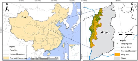
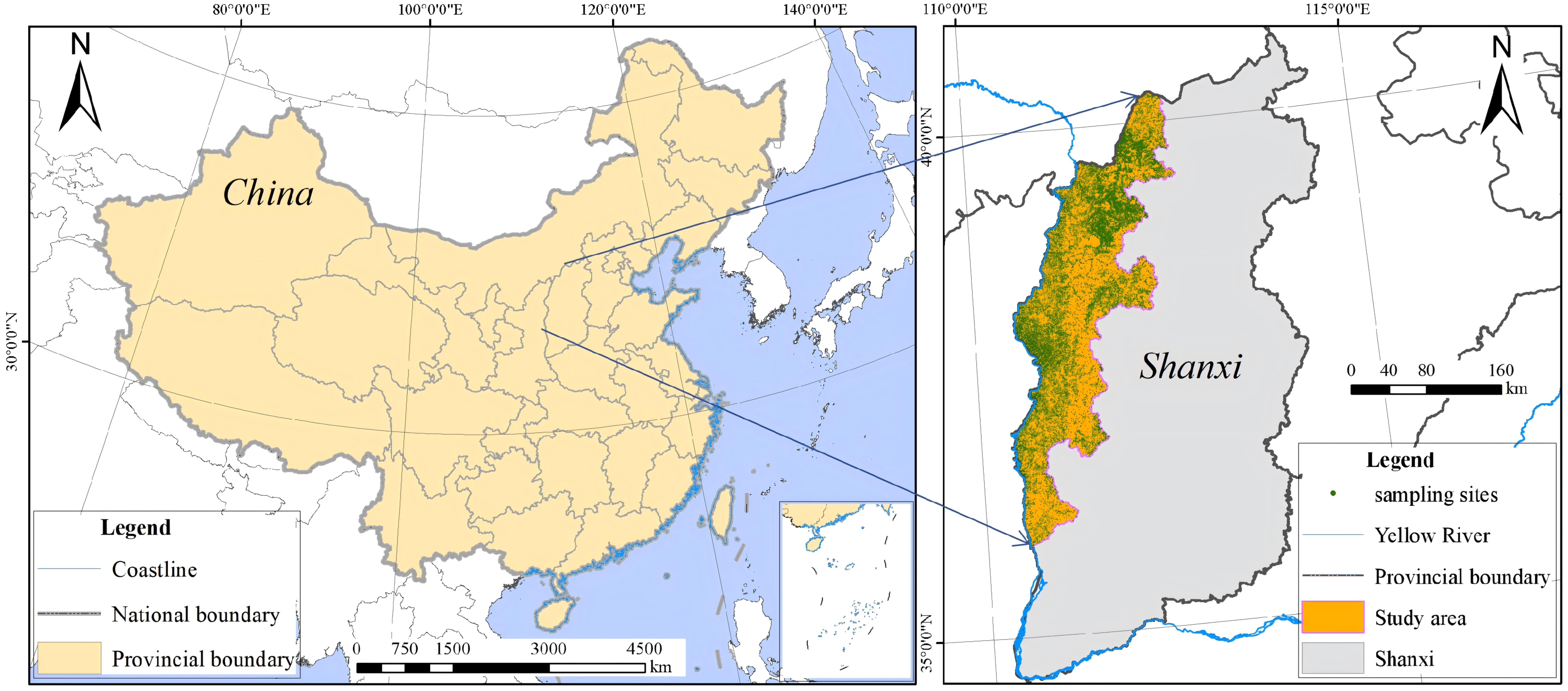
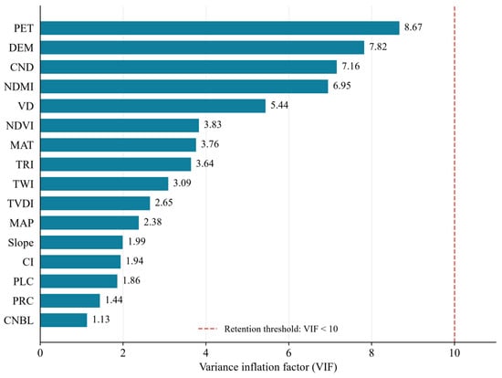
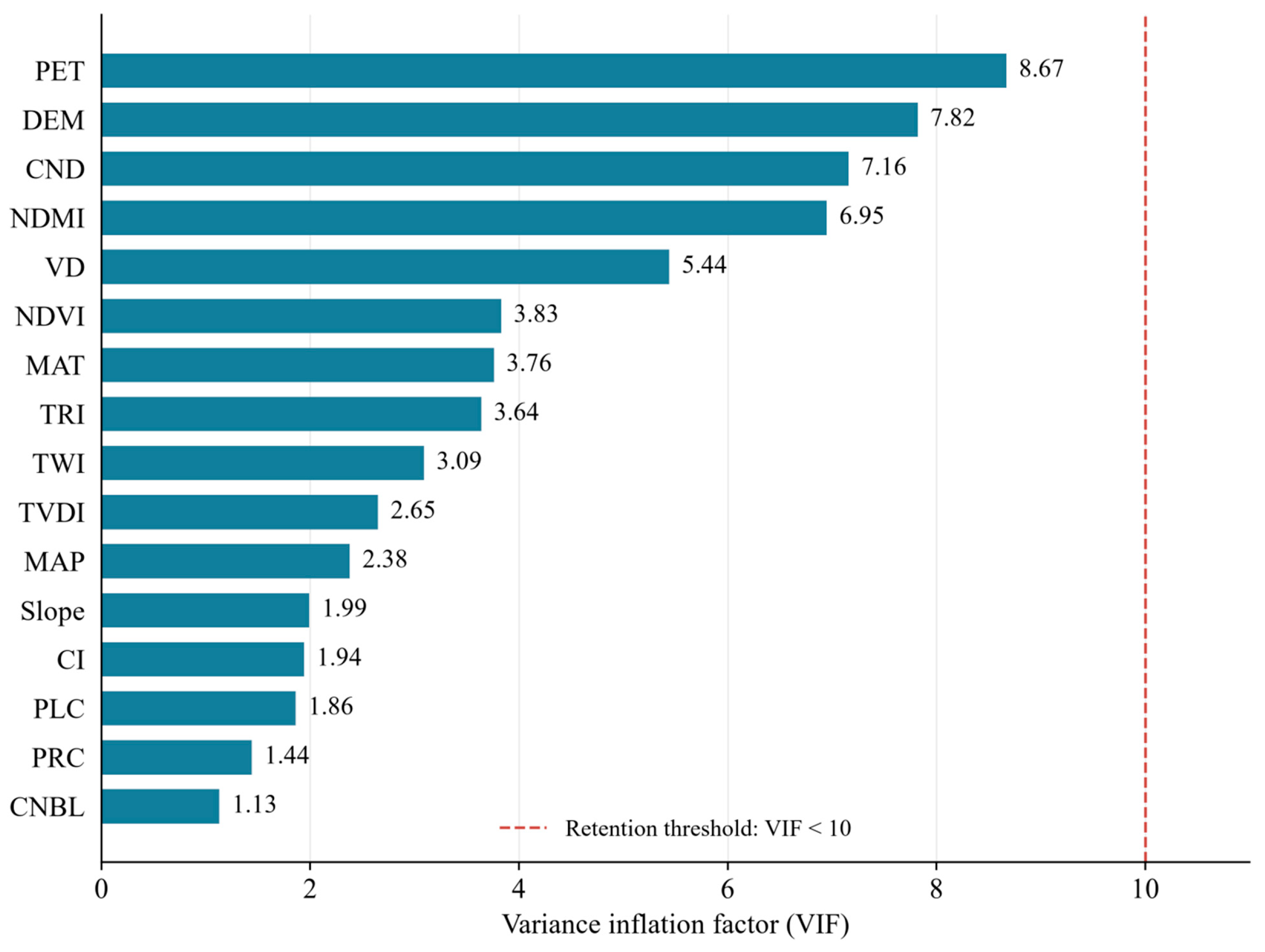
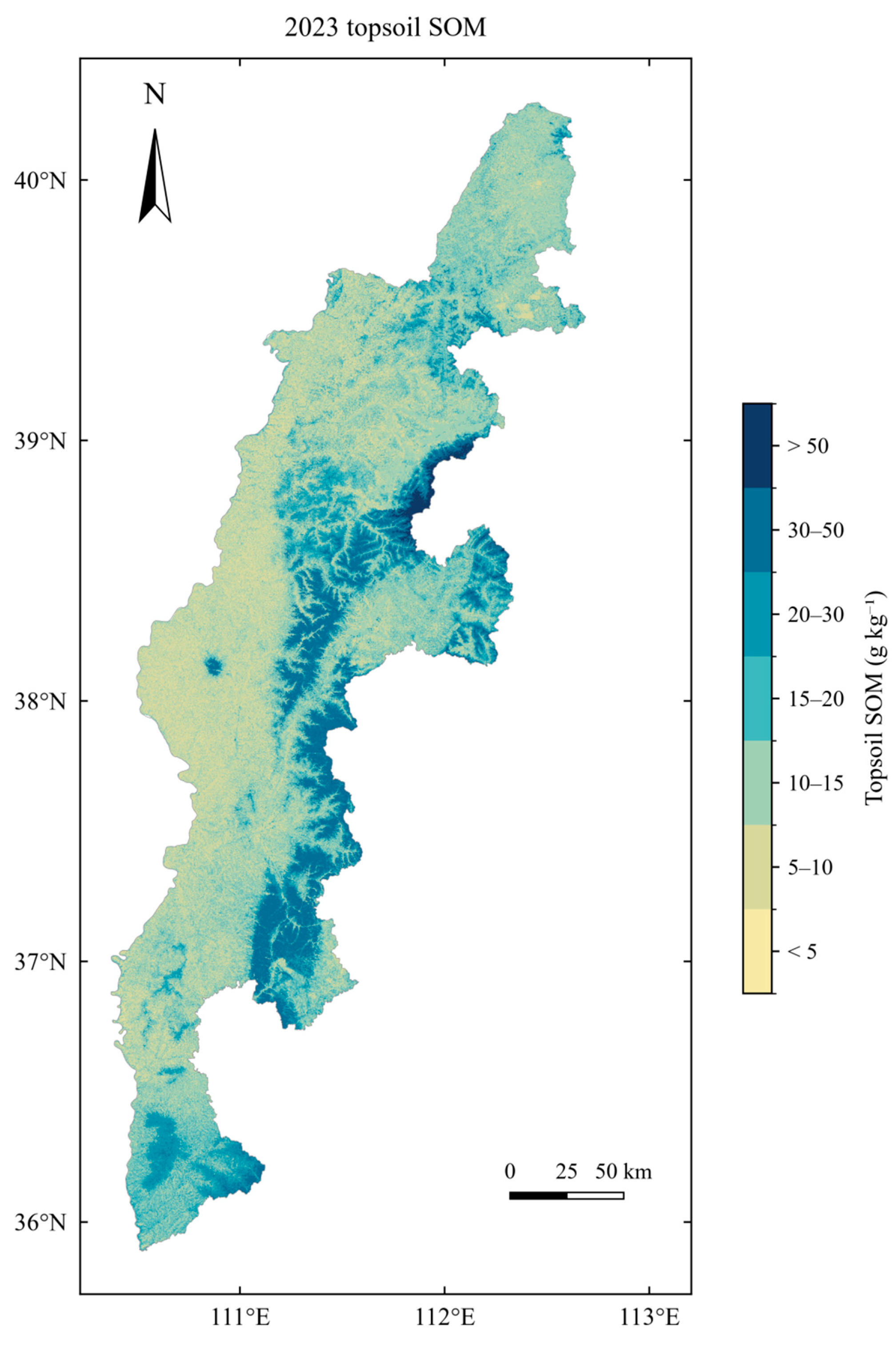
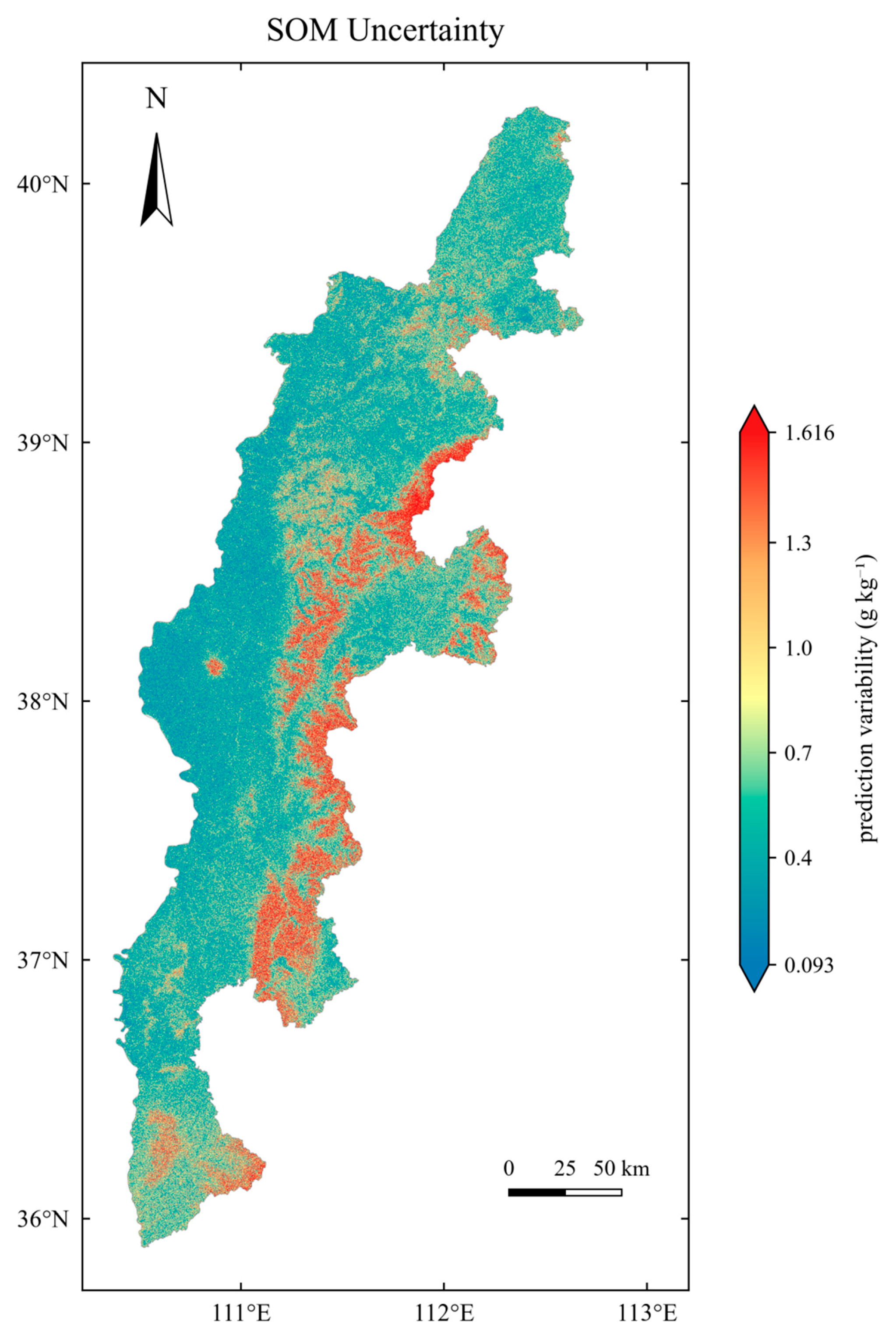
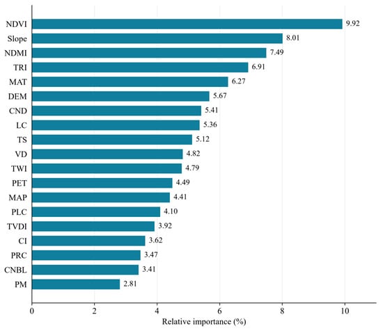
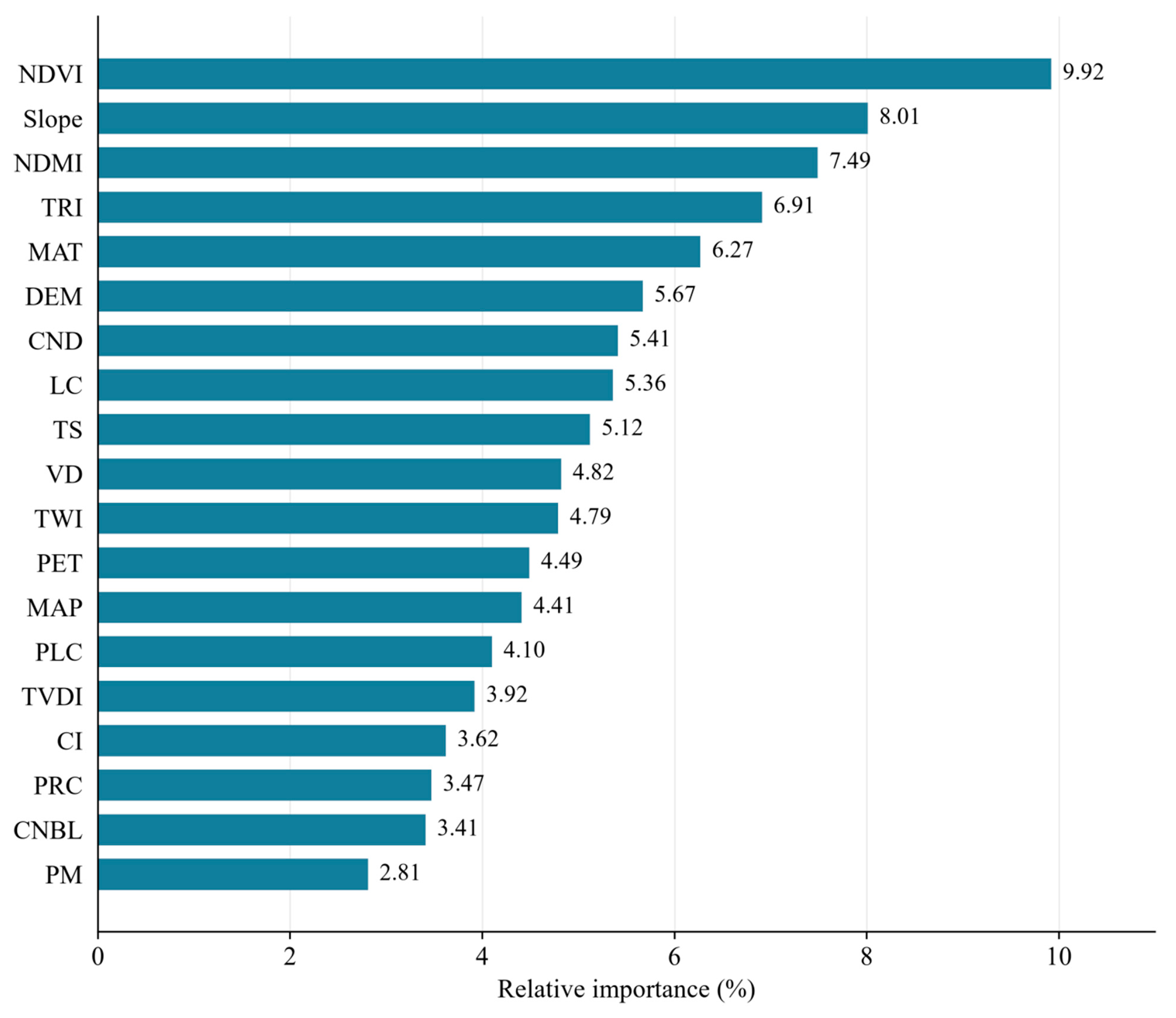
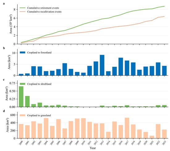
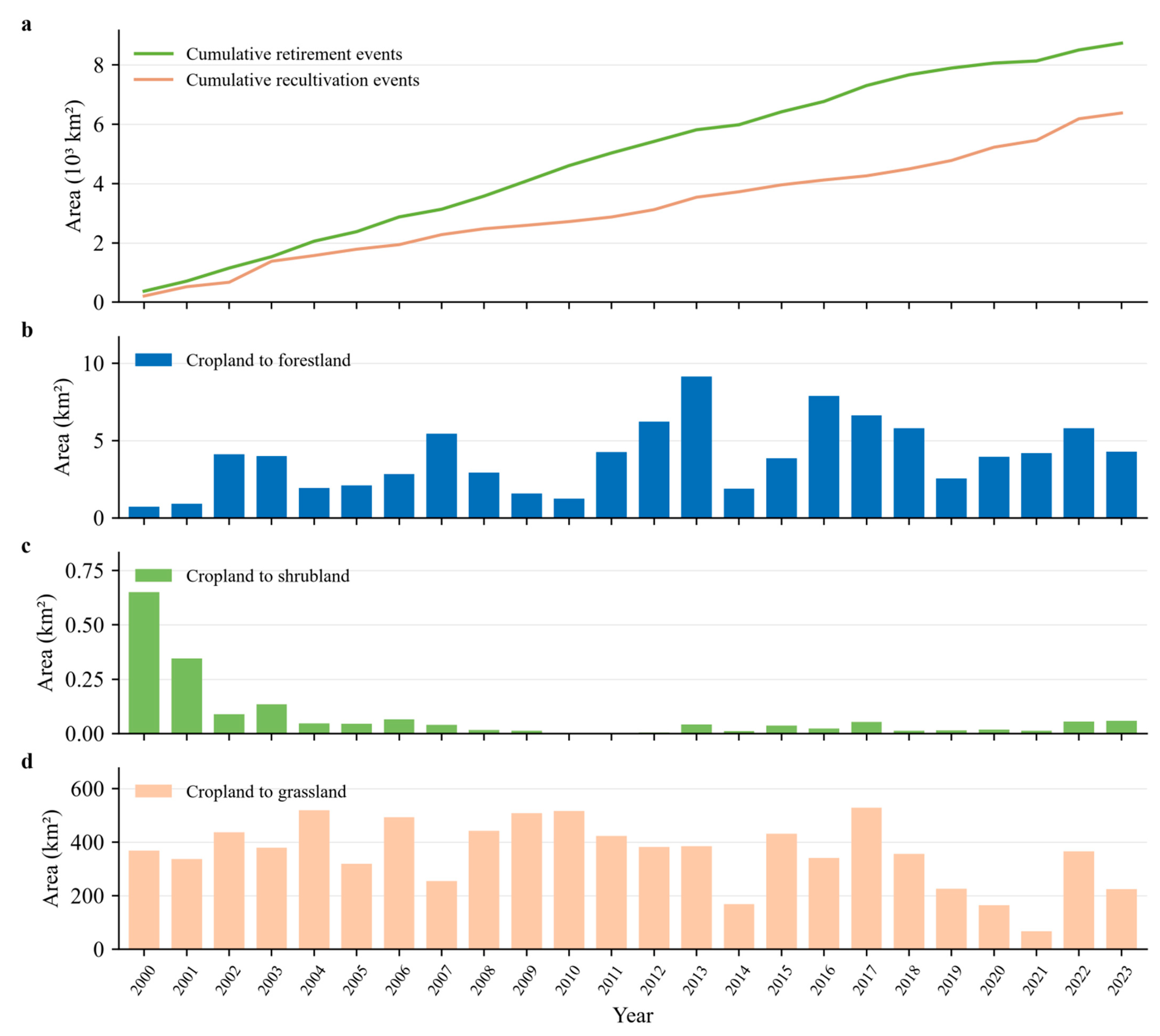
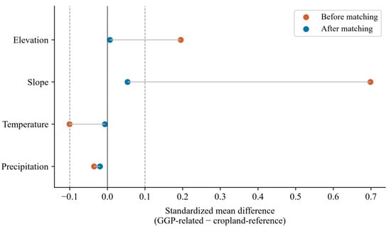
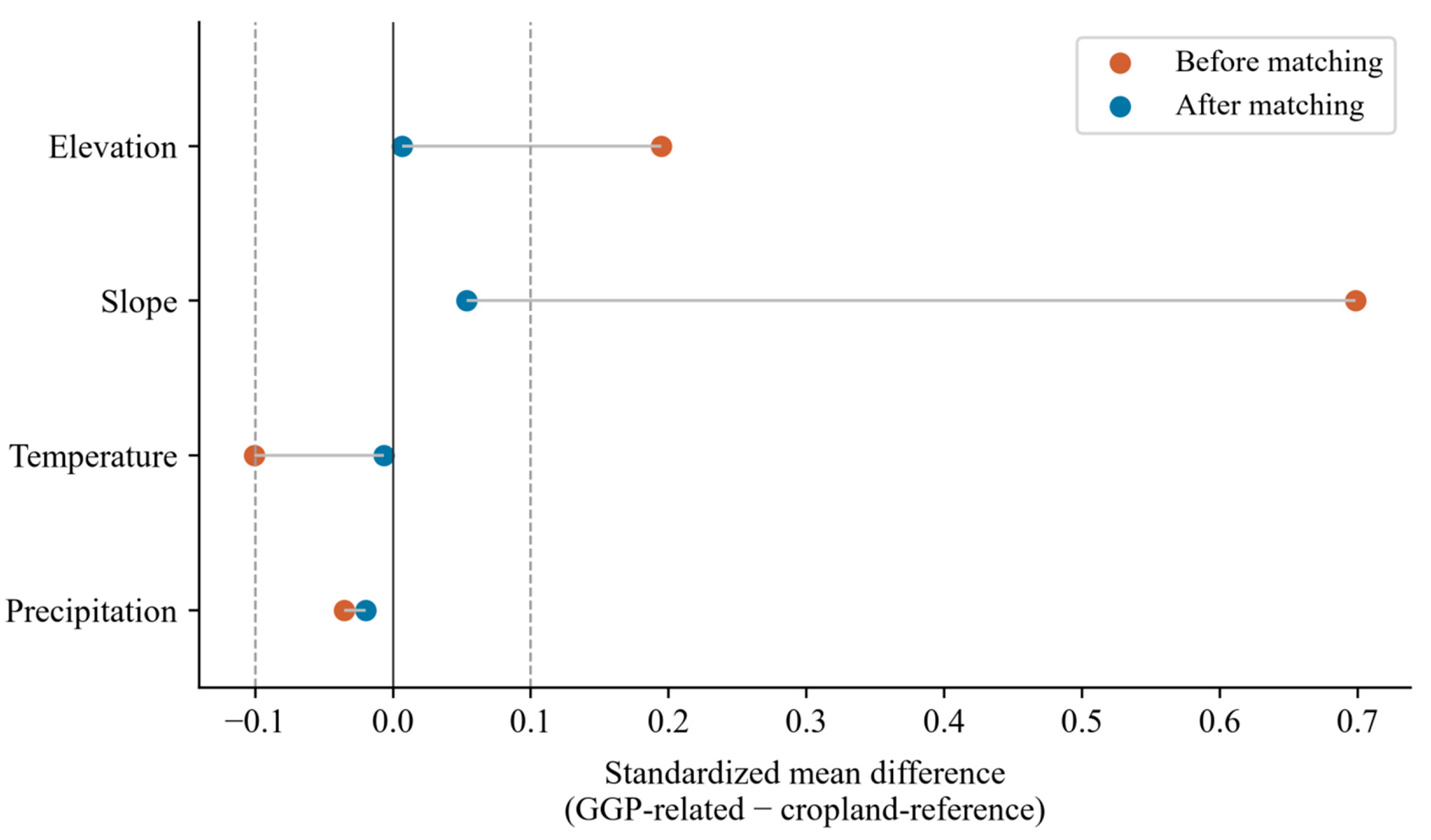
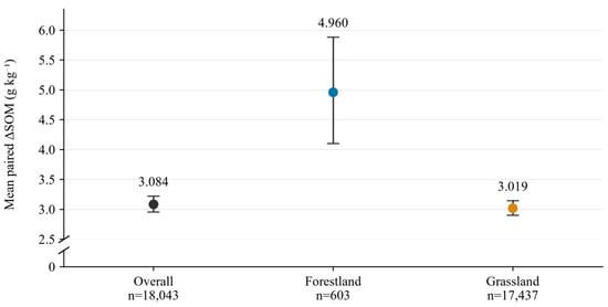
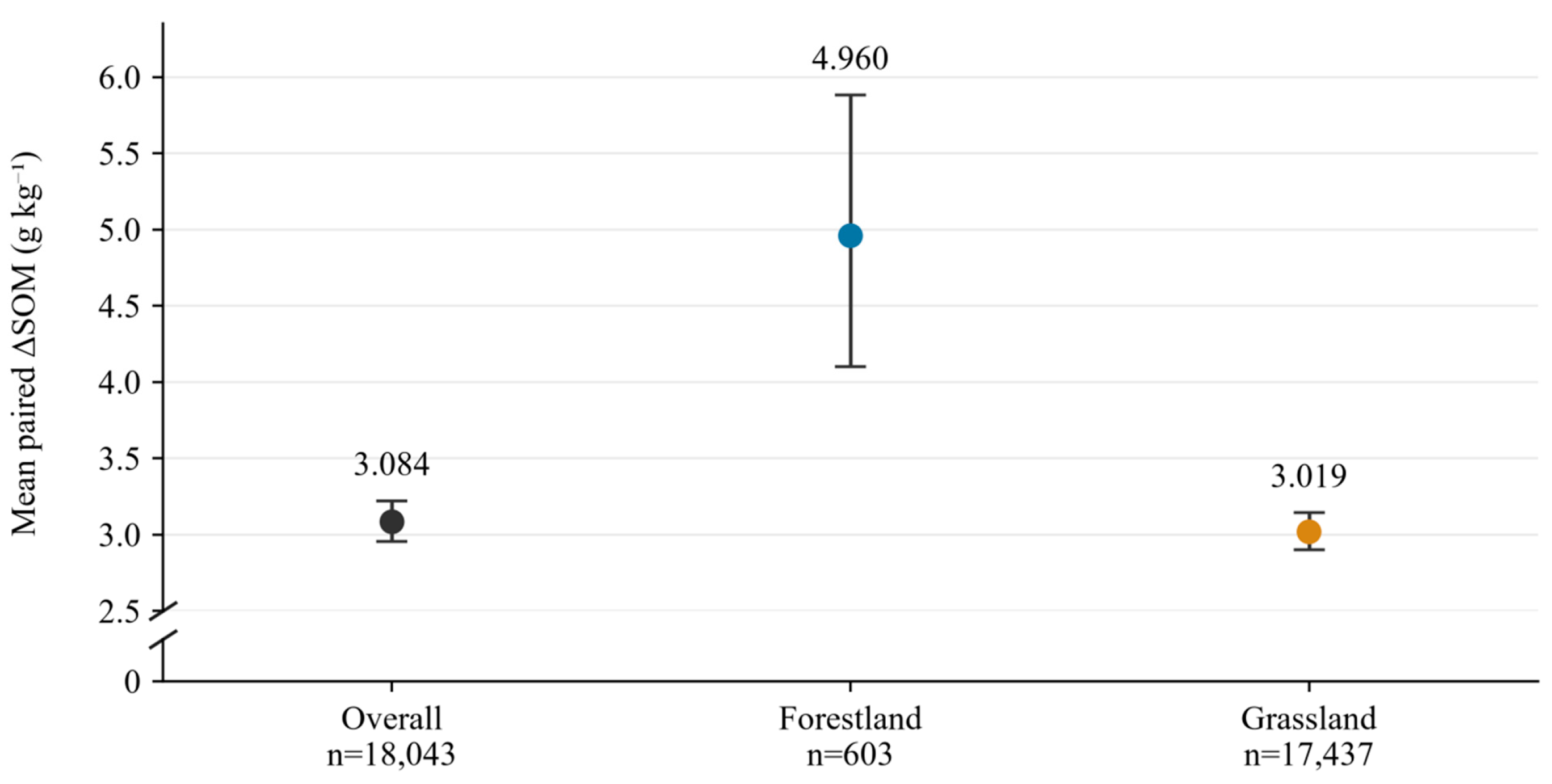
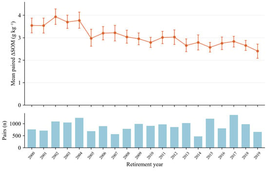
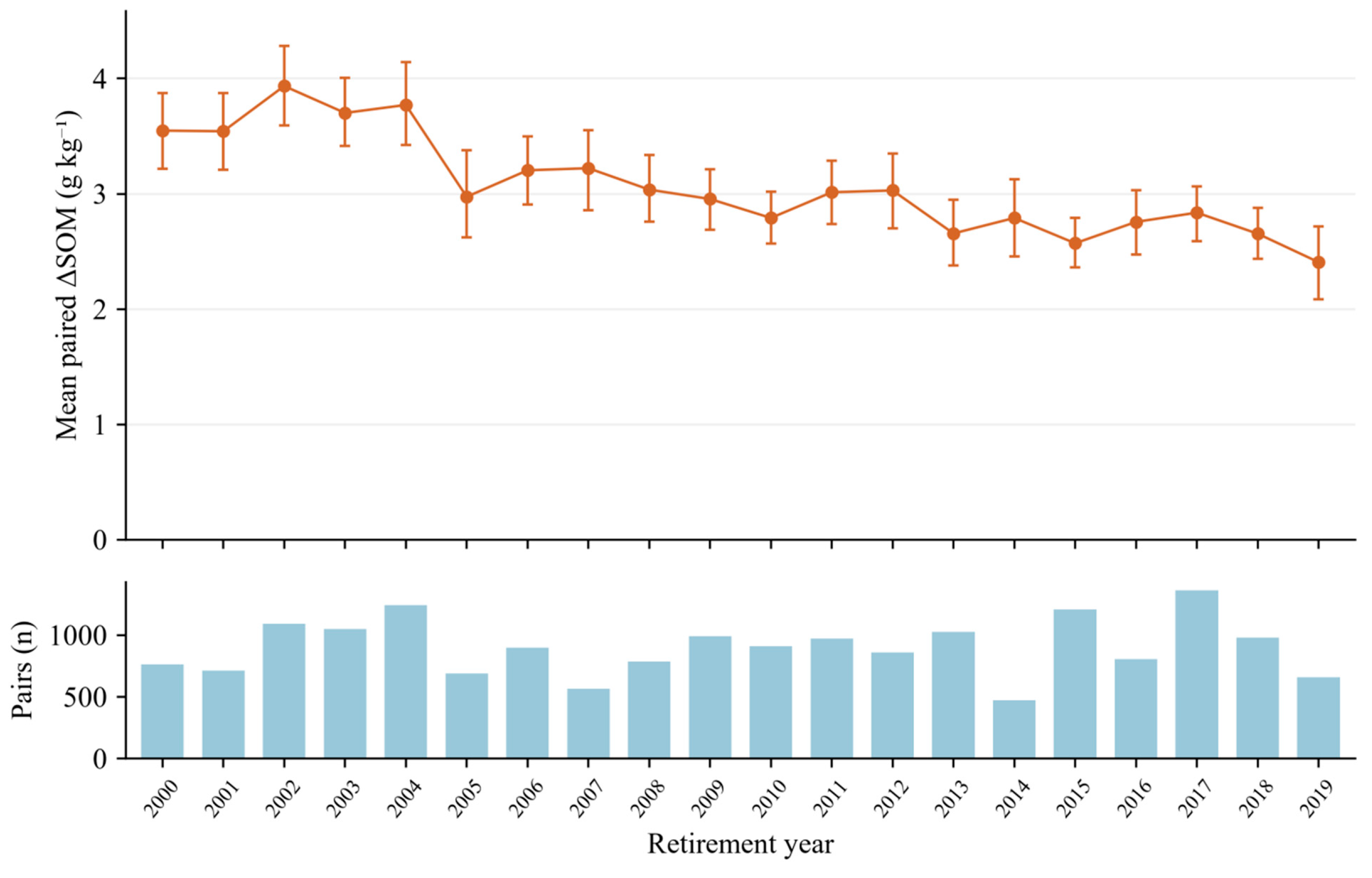
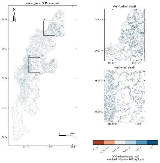
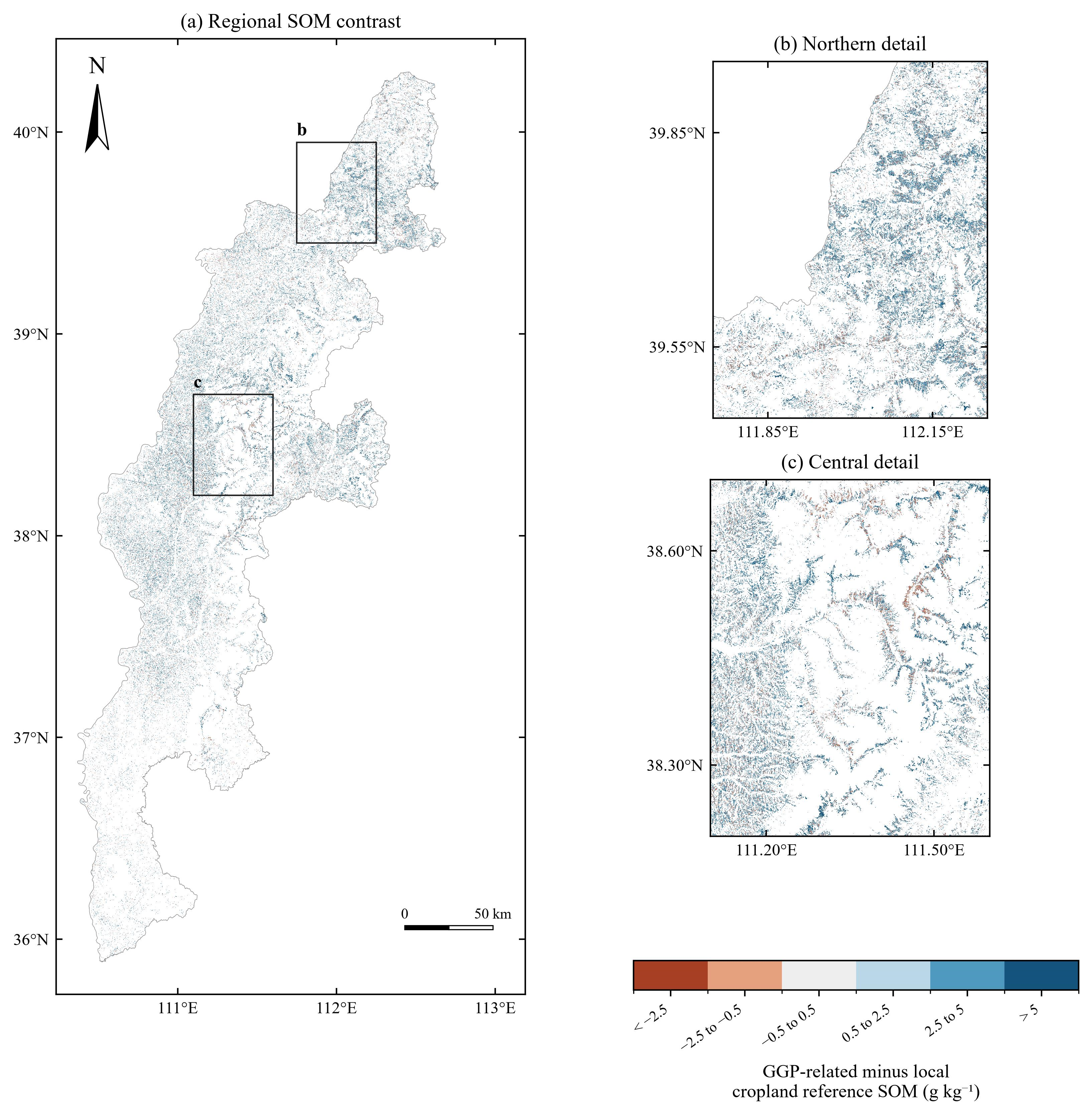

Disclaimer/Publisher’s Note: The statements, opinions and data contained in all publications are solely those of the individual author(s) and contributor(s) and not of MDPI and/or the editor(s). MDPI and/or the editor(s) disclaim responsibility for any injury to people or property resulting from any ideas, methods, instructions or products referred to in the content. |
© 2026 by the authors. Licensee MDPI, Basel, Switzerland. This article is an open access article distributed under the terms and conditions of the Creative Commons Attribution (CC BY) license.