


Abstract
The shoe last is central to footwear design. Modern footwear CAD operates on parametric digital lasts, yet much last geometry—legacy collections and lasts that skilled last makers still sculpt by hand and copy by pantograph turning—exists only as physical models or as point-cloud scans lacking the structured parametric form that footwear CAD requires. This paper presents a complete template-based method for reconstructing a watertight parametric last from a segmented point cloud without intermediate triangulation. The only manual input is three landmark points—for which the system proposes standard positions—and the interactive confirmation of two boundary lines on the digitized last. From these, the method defines four feature points, a median plane, and a four-curve boundary network; all subsequent stages run without user interaction. A curvature-adaptive quadrilateral grid is constructed on the cloud by geodesic tracing and monitor-weighted area-orthogonality relaxation. A periodic Coons tube interpolates the grid and initializes the parameterization for a periodic tensor-product cubic B-spline surface fitted by penalized least squares with cyclic/open difference penalties, exact boundary interpolation, and toe-aware weighting. Cap surfaces close both collar and sole openings, and the model is exported as a watertight B-rep solid. Tests on sixteen industrial lasts using one fixed parameter set produced a mean one-sided deviation of 0.034 mm (RMS 0.058 mm) from the withheld industrial reference meshes in approximately 12 s per last. With synthetic noise at 50 dB SNR, the mean deviation increased by only 0.011 mm. A sampling-density study indicated near-second-order convergence before the control-net reaches an upper limit. The resulting solids import directly into CAD systems and support re-lasting, footwear design, and customization.
1. Introduction
The shoe last is the physical or digital form around which a shoe is designed and manufactured. It carries both the geometry of the intended style and the anthropometric characteristics of the target population, and it supports downstream activities ranging from upper design and flattening to sole and mold engineering [1,2]. Modern footwear CAD/CAM systems use digital lasts, yet much geometric knowledge remains embodied in physical artifacts, including legacy collections, hand-sculpted design masters, and customized lasts produced through repeated manual correction, as well as lasts reproduced by pantograph copying; hand craftsmanship remains an active practice in last making, so such physical artifacts are not only inherited but continue to be produced. Converting these shapes into high-quality parametric CAD models is a routine but demanding task known in the industry as re-lasting, or last reverse engineering.
Three-dimensional scanning has made data acquisition inexpensive and reliable [3]. Optical scanners can produce dense point clouds of a physical last within minutes, and related scanning technologies support foot digitization for footwear customization [4,5], medical modeling and printing [6,7], and the digitization of cultural artifacts [8]. The main bottleneck is therefore surface reconstruction rather than measurement. The required output is a compact, watertight, high-continuity parametric model that CAD/CAM systems can use directly for grading, flattening, tool-path generation on free-form surfaces [9,10], and numerically controlled machining of the physical last.
Generic surface reconstruction methods typically produce triangle meshes or implicit surfaces. Although these representations can reproduce shape accurately, they do not provide the structured, low-degree parametric form required by footwear CAD. Quadrangulation and quad-layout techniques [11,12,13,14,15,16] generate all-quadrilateral connectivity suitable for spline fitting, but they target arbitrary topology and do not exploit the strong shape prior shared by shoe lasts: a smooth, approximately convex tube bounded by the feather and collar lines and characterized by standard anatomical landmarks such as the toe, heel, and cone. Template-based reverse engineering [17,18,19] uses this prior by fitting a parametric template with the required topology and semantics to the scan, thereby producing a semantically structured CAD model rather than only a reconstructed surface.
This paper presents a template-based methodology for reconstructing shoe lasts from segmented point clouds. The input is partitioned into body (tube), sole, and collar regions together with the two closed lines that separate them. The output is a closed, watertight parametric model whose main body is a single periodic tensor-product B-spline surface with continuity throughout, including across the periodic seam.
The pipeline has six steps (Figure 1). Step 1 instantiates four anatomical feature points, a median plane, and a locked boundary network. Step 2 constructs a curvature-adaptive, boundary-conforming quadrilateral grid directly on the point cloud by recursive subdivision, surface geodesic tracing, and weighted elliptic relaxation. Step 3 interpolates the grid with a Coons tube. Step 4 fits a periodic -continuous B-spline tube to the cloud by penalized least squares. Step 5 closes the sole and collar openings with cap surfaces, and Step 6 exports a watertight B-rep solid. Figure 2 illustrates the complete sequence for one last.
Figure 1.
The six-step re-lasting pipeline. Step 1 prepares the template entities on the input cloud; Steps 2–4 construct the tube surface (Steps 2 and 4, highlighted, carry the main computational content); Steps 5 and 6 close and export the watertight model.
Figure 2.
The reconstruction of the Allstar men’s last, end to end: (a) the physical last; (b) the segmented input cloud; (c) the initial depth-3 grid; (d) the same grid after adaptive refinement and weighted-AO relaxation; (e) the Coons tube interpolating the relaxed grid, shown with the grid overlaid; and (f) the fitted tube closed by the two caps. Panels (g,h) show the zebra and reflection maps of the exported solid in a commercial CAD system (Onshape), where the continuity of the tube—including the periodic seam—is visible as unbroken stripes.
The main contributions are the following:
- a template-based reconstruction pipeline for shoe lasts that operates directly on the point cloud: no intermediate triangulation is required at any step, since curve tracing, grid generation, relaxation, and fitting all rely on local neighborhood operators defined on the discrete sample;
- a curvature-adaptive quadrilateral grid-generation scheme (Step 2) that combines recursive subdivision, discrete geodesic tracing, and a monitor-weighted area-orthogonality (AO) elliptic relaxation constrained to the point cloud, with an interval-based adaptive refinement pass;
- a penalized fair-fitting formulation (Step 4) that combines a cyclic/open two-dimensional difference penalty of the Eilers–Marx type [20,21] with density-equalizing weights, coverage gating, and exact rim constraints, yielding a single periodic -continuous B-spline tube;
- an end-to-end evaluation on sixteen industrial last models, including a controlled noise experiment and a sampling-density study that indicates near-second-order convergence in the uncapped regime. After the manual template initialization—three landmark points and the confirmation of two boundary lines—the pipeline runs without user interaction in approximately 12 s per last on an AMD Ryzen 5950X and achieves sub-tenth-of-a-millimeter mean accuracy.
From a 3D computer vision perspective, the proposed pipeline performs shape recovery from range-derived point data: it transforms an unorganized, segmented point cloud into a structured, watertight parametric surface while preserving object-specific landmarks and boundary curves. It thereby links point-cloud processing and geometric reconstruction with a semantically organized representation suitable for downstream CAD and manufacturing applications.
The remainder of the paper is organized as follows. Section 2 reviews related work. Section 3 defines the input data model, the geometric entities of the last template and the reconstruction problem, and outlines the pipeline. Section 4 describes the preparation stage (Step 1). Section 5, Section 6 and Section 7 develop the mathematical core of the method: the adaptive tube grid (Step 2), the Coons tube surface (Step 3) and the P-spline fair fit (Step 4). Section 8 covers the closure and CAD export stages (Steps 5 and 6). Section 9 presents the implementation, including flowcharts of the three stages that carry the algorithmic control flow. Section 10 reports the experimental results and Section 11 concludes.
2. Related Work
Curves and projections on point clouds. Direct processing of unorganized point sets requires two robust primitives: projection of a moving point onto the sampled surface and curve tracing across that surface. The directed projection operator of Azariadis and Sapidis [22] projects a point by minimizing the weighted squared distance to the local neighborhood. Later work introduced automatic least-squares projection [23] and curvature-guided drawing on volumetric grids [24]. Point-cloud smoothing with shrinkage-free two-step filters extends Taubin’s mesh filter [25] through elliptic Gabriel neighborhoods [26]. The present pipeline combines these primitives: grid curves follow the point-to-point geodesic formulation of [27], whereas planar section curves use the plane-constrained formulation of [28]. Both formulations minimize tangential second-difference energy and repeatedly reproject the curve onto the cloud.
Geodesics on discrete geometry. Geodesic computation on meshes is a mature field, from the fast-marching solution of the eikonal equation [29] and exact polyhedral algorithms [30] to approximation schemes on weighted surfaces [31,32] and the heat method [33]; comprehensive surveys are available [34]. Fewer works address geodesics directly on point clouds [27,35]; the graph-seeded geodesic-curvature flow used throughout this paper belongs to this family and requires no surface triangulation.
Quadrangulation and structured grids. All-quadrilateral layouts have been constructed through spectral surface quadrangulation [11,12], Morse–Smale and Morse-parameterization methods [13,36], and global parameterization on meshes or directly on point clouds [14,15,16]. These methods target arbitrary topology and derive their layouts mainly from differential-geometric information. The proposed method instead prescribes the quad layout from the shoe-last template as two four-sided regions joined into a periodic tube, and focuses on placing that grid effectively on the cloud. It adapts structured grid generation—Winslow’s homogeneous elliptic smoothing [37] and Knupp’s area-orthogonality functional [38]—to a surface-constrained setting through the cloud-projection operator.
Spline fitting of scanned data. Least-squares fitting of tensor-product B-splines to measured points is classical [39,40,41], and the parameterization of the samples is known to dominate the achievable quality [42,43]. Recent contributions optimize the knot placement and the parameterization with metaheuristic search for engineering-scale fits [44], and the assembly of the least-squares matrices for large tensor-product spline fits has itself been accelerated substantially [45]. Fairness is usually enforced either through energy functionals on the surface or through discrete penalties on the control net. The P-spline approach of Eilers and Marx [20] penalizes finite differences of the coefficients and extends naturally to large tensor-product grids [21], while local energy fairing acts on individual control points [46]. Implicit spline representations offer an alternative reconstruction route: hierarchical implicit B-splines recover closed surfaces from point clouds through phase-field guidance [47] or low-rank tensor approximation [48], although the result is an implicit rather than a parametric CAD surface. Step 4 adopts the P-spline formulation with a cyclic difference penalty in the periodic direction, applied to a fully three-dimensional, surface-valued fitting problem with landmark and boundary constraints.
Footwear CAD and template-based reverse engineering. Last design and customization have been studied extensively, including last generation from foot measurements [1,5], fit assessment between feet and lasts [2,49], free-form-deformation morphing of last families [18], and volume-parameterization approaches for the design automation of customized free-form products [19]. Recent work continues this line with feature-based systems that construct customized last models from three-dimensional foot scans inside CAD environments [50]. On the reverse-engineering side, template-based strategies fit parameterized CAD templates to scans of mechanical parts [17]. More recently, learning-based reverse engineering has been proposed to recover procedural CAD programs directly from point clouds [51]; such methods address prismatic, sketch-and-extrude engineering parts, whereas the last requires a single free-form, semantically structured surface. In contrast to these approaches, the methodology presented here uses the last template not as a library shape to be deformed but as a topological and semantic prior—four landmarks, two feature curves and the two committed boundary lines. Three components distinguish it from prior template-based reconstruction: every stage operates directly on the point cloud, so no triangulation is built at any step; structured elliptic grid generation, in the sense of the Winslow and area-orthogonality functionals, is carried over to point clouds to produce the curvature-adaptive tube grid of Step 2; and the fit of Step 4 delivers a single periodic B-spline tube with exact rim interpolation and a cyclic difference penalty, so that the result is a fair, watertight, and semantically structured model suitable for direct CAD exchange [52]. Point-cloud analysis tools relevant to the preparation stage include protrusion-oriented semantic segmentation [53] and feature enhancement in noisy clouds [54].
3. Problem Statement and Pipeline Overview
3.1. Input Data Model
The input is a digitized shoe last, represented by a point sample of its boundary surface and partitioned into three region clouds expressed in a common coordinate frame (Figure 3): the body cloud , which samples the lateral tube-like surface of the last; the sole cloud , which samples the bottom; and the collar cloud , which samples the top cap. The partition is delimited by two closed curves lying on the sampled surface: the feather line , the sharp free edge where the body meets the sole, and the collar line , which bounds the top opening. Both lines are given as ordered closed polylines and are interpolated by periodic cubic curves , . Segmented inputs of this kind are produced routinely by last-digitization hardware and software and can also be derived from raw scans by point-cloud segmentation [53].
Figure 3.
Input data model and template entities on the Allstar men’s last (12,455 points): the body (blue), sole (orange), and collar (green) region clouds; the feather line and collar line ; the mid curve (→ ) and heel curve (→ ); and the four feature points , , , and .
Each body point carries a unit normal , either measured or estimated by local principal component analysis (PCA) of its -nearest-neighbor set ( throughout) and globally oriented by minimum-spanning-tree propagation. Two derived quantities are used throughout the paper. The first is the mean point spacing , the average nearest-neighbor distance over the cloud, which serves as the intrinsic length unit in which all tolerances are expressed. The second is the -nearest-neighbor graph with Euclidean edge weights, which supports the A* shortest-path queries that seed all curve tracing.
Two local operators give the cloud the structure of a sampled surface. The first is the directed projection operator [22], which projects an arbitrary point onto the local weighted cloud neighborhood. Let be the -nearest cloud points of , let be Gaussian weights, let be the weighted centroid of these neighbors, and let be their unit weighted average normal. Then
The neighborhood may optionally be filtered to its elliptic Gabriel subset [26]. Because is a first-order moving-least-squares projection, it varies smoothly with , which is the property the iterative solvers of Steps 2–4 rely upon.
The second operator traces geodesics on the cloud, that is, it produces a taut curve on the sampled surface between two fixed endpoints. A discrete curve is a discrete geodesic when the tangential component of its second difference vanishes, so the operator minimizes the discrete geodesic-curvature energy [27]
where is the local surface normal at . The curve is initialized by the A* shortest path on the neighborhood graph and resampled uniformly by arc length. Each outer iteration then (i) solves the normal equations of Equation (2) for the interior points by matrix-free conjugate gradients, (ii) reprojects the interior points onto the cloud with Equation (1) and refreshes their normals, and (iii) applies the two-pass Taubin filter [25]. The first pass uses the positive weight and the second uses the negative weight , with
The two passes filter low-spectrum noise of the polyline without shrinkage. The iteration stops when the squared curve length stabilizes. A plane-constrained variant alternates the same operations with orthogonal projection onto a prescribed plane, so that the curve converges to a discrete sampling of the intersection between the sampled surface and that plane [28]. This variant is used for the planar feature curves of Step 1. Table 1 summarizes the global notation used throughout the paper.
Table 1.
Global notation. Symbols used within a single stage are defined where they first appear.
3.2. The Last Template and the Reconstruction Problem
The template of a shoe last consists of four feature points, two feature curves and the two boundary lines (Figure 3). The toe point () and the heel-bottom point () lie at the front and the rear of the feather line, the cone point () and the heel-top point () at the front and the rear of the collar line; Section 4.1 gives their exact definition. The mid curve joins to across the instep and the heel curve joins to up the back of the last. Both lie on the median plane, the plane through , and , which separates the last into its medial and lateral halves. Together these entities partition the body surface into two four-sided curvilinear regions, the medial and the lateral side. Each region is bounded by a feather arc, a collar arc, the mid curve and the heel curve, with the four feature points as corners. Glued along and , the two sides form a topological cylinder, an open tube whose rims are the feather and collar lines.
The reconstruction problem is stated as follows. Given the segmented cloud with its two boundary lines, construct (i) a single parametric tube surface , periodic in , that approximates fairly and with continuity everywhere, including the periodic seam, while interpolating the feather and collar lines as its boundary curves and respecting the template landmarks; and (ii) two cap surfaces closing the sole and collar openings, so that the complete model is exactly watertight and exportable as a manifold CAD solid. The feather line of a physical last is a sharp crease by design. The caps are therefore required to join the tube with positional () continuity along the rims, and all smoothness requirements concentrate on the tube itself.
3.3. Pipeline Overview
Figure 1 summarizes the six steps. Step 1 is the preparation stage: from three interactive picks it instantiates the template entities on the given cloud, namely the feature points, the median plane and the locked boundary-curve network. Step 2 constructs a boundary-conforming quadrilateral grid on the body cloud by recursive subdivision with on-cloud geodesic tracing, refines it adaptively where the size or curvature criteria demand, and then improves it by a curvature-weighted, surface-constrained elliptic relaxation. Step 3 interpolates the relaxed grid by a periodic Coons tube surface as a first-order-continuous parameterization scaffold. Step 4 replaces interpolation by approximation: a periodic tensor-product cubic B-spline tube is fitted to the cloud by penalized least squares, with the Coons tube serving as the initial parameterization reference, and the result is the final -continuous body surface. Step 5 closes the two openings with cap surfaces, with the sole cap additionally fitted to the sole cloud by a smooth displacement field. Step 6 assembles and exports the watertight solid. Steps 2 and 4 contain the main mathematical developments and are detailed in Section 5 and Section 7.
4. Step 1: Preparation—Feature Points, Median Plane, and Boundary Network
4.1. Feature Points and Median Plane
The template is instantiated from three points picked on the two boundary lines; the fourth feature point is extracted. The system proposes standard initial positions: the heel-bottom point at the start of the feather line, , the toe point at its halfway parameter, , and the heel-top point at the start of the collar line, . The designer may slide any of the three points along its own line when the style of the last requires it. No other quantity is adjustable at this stage.
The toe–heel chord axis
orients the last. The three picked points then determine the median plane directly, as the plane through , , and :
The unit normal is well defined whenever the three points are not collinear, a condition satisfied by the last geometry. The signed distance to defines the side function
which labels the medial () and the lateral () half of every entity. Because the plane is pinned to three landmarks rather than optimized, it is reproducible: the same three picks always give the same median plane, and moving one pick moves the plane predictably.
The remaining feature point is derived. The cone point is the frontmost crossing of the median plane with the collar line. Consecutive samples with opposite signed distances bracket a crossing, which is resolved by linear interpolation, and among those crossings
is the one furthest forward along the chord axis. Finally, the two feature curves are traced with the plane-constrained geodesic operator of Section 3.1 [28]: the mid curve from to , and the heel curve from to . Each is a polyline lying on the intersection of the sampled surface with . These paths are constrained to the median plane rather than being unconstrained shortest paths. This constraint makes them reproducible template landmarks while keeping them on the sampled surface.
4.2. The Committed Boundary Network
The preparation ends by turning these entities into the committed boundary network that all later steps use. The tube surface is periodic across the front seam, so neither boundary line may have a tangent discontinuity where it closes. Each line is therefore re-anchored at its front feature point, the feather line at and the collar line at , and its two ends are corrected to meet with tangent-direction () continuity.
Let and be the unit tangent vectors of the two branches of the line that leave and enter the closure point. The common target tangent is their normalized bisector , and the samples near each end are rotated about the anchor by a tapered Rodrigues rotation,
where denotes the rotation by angle about the axis , and is the angle between the end segment and the target tangent. The taper spans the samples nearest the closure, about 4% of the samples of the line. The rotation decays linearly along the taper, so the correction is local and the shape of the line is otherwise preserved.
Both lines are then adjusted to pass exactly through their two feature points, after which the network is locked. The corrected feather and collar lines become the committed boundary curves, represented as periodic Catmull–Rom interpolants of their polylines; the mid and heel curves are stored as interior feature rails; and the four feature points become the fixed corners of the two side regions. Each side of the locked network is bounded by four curves: its feather arc (), its collar arc (), the shared mid curve (), and the shared heel curve (). This is the input required by the grid construction of Step 2. Once this initialization is complete, all remaining stages run automatically.
5. Step 2: Curvature-Adaptive Quadrilateral Tube Grid
Step 2 constructs a structured quadrilateral node lattice that lies on the point cloud, conforms to the committed boundary network, and is distributed so that the grid resolution follows the surface curvature. It proceeds in three phases: recursive subdivision (Section 5.1), stitching into a periodic tube (Section 5.2) and surface-constrained elliptic relaxation (Section 5.3), optionally followed by adaptive refinement (Section 5.4).
5.1. Recursive Boundary-Conforming Subdivision
Each of the two side regions of the tube is treated as a curvilinear quadrilateral patch with boundary curves , , , (bottom = feather arc, top = collar arc, left = mid curve, right = heel curve), each an on-surface polyline parameterized by normalized arc length. One subdivision level splits the patch into four children (Figure 4a). The arc-length midpoints , , , are computed, and the patch center is estimated as their average and snapped to the nearest cloud point . Four new interior grid curves , , , are then traced on the cloud with the geodesic operator of Section 3.1, each boundary curve is split at its midpoint, and the construction recurses on the four children down to a prescribed depth . Every child inherits exact sub-arcs of its parent’s curves, so the subdivision is boundary-conforming by construction. After levels, each side carries a lattice of nodes with ; the default gives nodes per side.
Figure 4.
The tube-grid domain of Step 2. (a) One level of the recursive boundary-conforming subdivision: arc-length midpoints (squares), the center point snapped to the cloud (open circle), and the four traced interior grid curves (dashed). (b) The two side lattices stitched into one periodic tube lattice: rows and are the feather and collar rims, columns and carry the mid and heel curves, and the column index wraps periodically.
The recursion normally fills the whole lattice. A branch may nevertheless stop early, either because a child patch becomes too small to subdivide or because one of its geodesic traces fails, and the lattice slots that it never reached are then left empty. Those slots are filled by the bilinearly blended Coons interpolant of the four patch boundary curves,
evaluated at the lattice parameters and projected onto the cloud with Equation (1); here are the four patch corners. The boundary rows and columns of the lattice are finally reset onto the committed boundary curves, so that the lattice conforms exactly to the network locked in Step 1.
The number of samples of each traced grid curve is proportional to its length: on an A* seed path of length , with by default, that is, one sample every two point spacings.
5.2. Stitching into a Periodic Tube
The medial and lateral lattices share their first and last columns, the mid and heel polylines, and are stitched into a single periodic lattice around the last (Figure 4b). With lateral nodes and medial nodes , the tube lattice is
which gives nodes with and quadrilateral cells. The column index is periodic modulo : column carries the mid curve, column (initially ) carries the heel curve, and rows and are the feather and collar lines. In what follows, and denote the logical grid coordinates along (around the tube) and (across it).
5.3. Surface-Constrained Elliptic Relaxation
The subdivision lattice is geometrically valid but generally uneven: cells shear where the boundary arcs have very different lengths, and the node density ignores curvature. The lattice is therefore relaxed by a nonlinear Gauss–Seidel iteration derived from variational grid generation, with every intermediate position constrained back to the sampled surface. At an interior node , central differences of the neighboring nodes define the discrete tangents and the metric coefficients
where denote the four edge neighbors of the node (periodic in ) and its four diagonal neighbors.
Winslow (harmonic) generator. The classical Winslow functional [37] yields the homogeneous elliptic system . Substituting the standard difference stencils and solving for the central node gives the Gauss–Seidel target
Area-orthogonality (AO) generator. The default generator is Knupp’s area-orthogonality functional [38]
whose Euler–Lagrange equations expand to , with and . This is the same principal part as Winslow’s system with a different first-order source. The corresponding target is
Compared with the harmonic map, the AO generator tends to distribute grid lines more uniformly while maintaining favorable crossing angles. In concave regions such as the instep, it also reduces the tendency of grid lines to cluster excessively.
Curvature-adaptive weighting. To concentrate resolution where the surface bends, the AO update is weighted by a monitor field derived from the principal curvatures , estimated per cloud point by local quadric fitting. With sampled at the cloud point nearest each node and its median over the lattice,
where (default 3) controls the strength of the adaptation and the cap prevents runaway clustering at sharp spots. The factor is an optional landmark multiplier: it equals 2 inside the toe box, a slab of prescribed depth behind the toe point along , and 1 elsewhere, which reflects the special fitting importance of the toe region. The field is smoothed by a few Jacobi passes of a five-point kernel. Interpreting the monitor as the diffusivity of an elliptic flux and discretizing with edge-averaged weights (and analogously for the other three edges) yields the weighted target
where is the ratio of the denominator to . The construction reduces exactly to Equation (15) for uniform . Balancing the weighted flux makes the local grid spacing scale as , so the grid lines cluster in regions of high curvature and inside the toe box. Every other factor of Equation (17) has already been introduced: are the four edge neighbors and the metric coefficients of Equation (12), are the central-difference tangents of Equation (11), are the edge-averaged monitor weights, and are the area-orthogonality source coefficients of Equation (15). The numerator blends the monitor-weighted neighbor averages of the two grid directions, and the denominator normalizes the same weights.
Relaxation sweep. One sweep updates every interior node in place. The target of Equation (17), or of Equation (13) for the harmonic generator, is blended with the isotropic Laplacian average using a small blending weight (default 0.15) that stabilizes the node spacing, and the node then moves by the under-relaxed step
with relaxation factor , the step length being capped by the local cell size. The constraint operator is what carries planar elliptic grid generation over to the sampled surface: free interior nodes are re-projected onto the cloud by Equation (1), while the nodes of the two feature columns ( and ) are projected onto the mid and heel polylines, so that the grid never leaves the template rails.
Boundary slide. Rim nodes ( and ) may move only along their own lines and are therefore updated in the line parameter . Two competing targets are blended. The orthogonality target is the parameter of the point closest to the position that would make the inward grid edge perpendicular to the line, computed in the local tangent plane. The spacing target is the monitor-weighted average of the parameters of the two neighboring rim nodes. The update
with default , preserves the strict cyclic ordering of the rim nodes through a minimum-gap safeguard. The blend removes the classical failure mode of pure orthogonality sliding, in which the rim nodes migrate toward the heel and leave the toe under-resolved. The four feature corners remain fixed.
Iteration control. Sweeps alternate interior updates and boundary slides until the maximum node displacement falls below , or until a prescribed maximum number of sweeps (default 300) is reached. The composition of Gauss–Seidel updates, surface projection and boundary sliding is not the gradient flow of a single functional, so a grid-quality functional is evaluated every few sweeps and the configuration with the best value is retained. The default functional penalizes deviations of the grid angles from ,
where is measured between on-surface secant tangents at each node and the bars denote means over the interior and the rim nodes. The four terms weight, in order, the mean angle error of the interior nodes, the mean error of the rim nodes, and the maximum single-node error of each of the two groups; the mean interior term therefore dominates the selection, while the two maximum terms penalize an isolated, strongly distorted node that a mean alone would conceal. The constant denominator only rescales the functional and does not affect which configuration is selected. On the test set of Section 10 the relaxation raises the mean interior grid angle from about to and the mean rim crossing angle from to on the Allstar last (Figure 5).
Figure 5.
Step 2 on the Allstar last: (a) the initial depth-3 grid (16 × 9 nodes); (b) after adaptive refinement (57 × 19 nodes)—columns cluster at the toe, rows along the feather line; (c) after weighted-AO relaxation—the mean interior grid angle rises from 61° to 82° while the curvature clustering is retained.
5.4. Adaptive Refinement
A second, criteria-driven subdivision pass, applied to the stitched tube of Section 5.2 before the relaxation of Section 5.3, adapts the lattice resolution to the data while keeping it structured. Complete grid intervals, that is whole columns or rows of cells, are split, so that the tube remains a tensor lattice and simply loses its power-of-two dimensions. With cloud spacing , curvature magnitude as above and cloud-wide median curvature , a column interval (and analogously a row interval ) of widest cell edge and largest incident curvature is split if and only if
with defaults , and . The floor guarantees that no child edge drops below and thereby stops runaway splitting at the sharp toe. Up to three passes are applied. The lattice size is bounded by a hard limit of 128 columns and 64 rows; when a pass requests more splits than the remaining room allows, the intervals with the largest violation are split first and the rest are dropped. New nodes are inserted through on-surface midpoints: interior edges receive the arc midpoint of a freshly traced geodesic, rim nodes are born on their lines and feature-column nodes on their rails, so every invariant of the relaxation is preserved and the refined lattice is then relaxed.
Figure 5 shows a typical grid before adaptive refinement, after refinement and after the weighted-AO relaxation. Note the clustering of columns at the toe and of rows along the feather line. Because the fitted control net of Step 4 is tied to the grid dimensions, refined bands translate directly into additional spline degrees of freedom exactly where the geometry demands them.
6. Step 3: The Coons Tube Surface
Step 3 converts the relaxed grid into one periodic, piecewise parametric tube surface that interpolates the grid curves. It serves both as a stand-alone reconstruction of the body and as the parameterization reference for the fair fit of Step 4. Let be global tube parameters, with periodic, so that cell occupies the rectangle and carries local coordinates .
A shared first-order data set is computed at every node: central-difference tangents, periodic in and one-sided at the rims,
with the corner twists set to zero. On the two rims the direction of is re-aimed along the committed boundary line, its magnitude being preserved, so that the rim edge curves of the surface follow the committed lines and the tangent field is single-valued across the periodic wrap. Each cell then carries a bicubically blended Coons patch [55] built from the four traced grid curves that bound the cell itself. With Hermite basis , those four bounding edge curves evaluated at arc-length fractions, and corner data , the patch is the Boolean sum
where lofts the bottom/top edge curves with linearly blended -tangent ribbons, lofts the left/right edge curves with linearly blended -tangent ribbons,
(and symmetrically for ), and is the bicubic Hermite tensor patch on the corner data that removes the doubly counted part,
Each patch reproduces its four edge curves exactly. The assembled tube is therefore watertight with positional () continuity across all cell boundaries and the periodic seam, and it interpolates the feather and collar lines. Adjacent patches share their common boundary curve and cross-boundary tangent data derived from shared node tangents. These data are single-valued at grid nodes and provide a near- transition along interior edges; however, small derivative mismatches may remain where composite grid curves change tangent. The Coons tube is therefore used as an interpolation and parameterization scaffold, whereas Step 4 provides global continuity. Figure 6a shows the Coons tube of the Allstar last with the underlying grid overlaid.
Figure 6.
The tube surfaces: (a) the bicubically blended Coons tube interpolating the relaxed grid (Step 3, 1026 patches, shown with the grid overlaid); (b) the final P-spline tube fitted to the body cloud with a 64 × 33 control net (Step 4).
7. Step 4: Penalized Least-Squares Fair Fit
The Coons tube interpolates the grid, but between the grid curves it only approximates the cloud, and the continuity of the patchwork is only first order. Step 4 raises the reconstruction to a single, globally -continuous parametric surface by fitting a periodic tensor-product cubic B-spline surface to the body cloud with a penalized least-squares (P-spline) formulation.
7.1. Surface Model
The fitted surface is
where are uniform periodic cubic B-spline basis functions in the around-the-tube direction, are clamped cubic B-spline basis functions on an open-uniform knot vector with simple interior knots in the feather-to-collar direction, and is the control net. All u-knots are simple and the control columns wrap cyclically, so the surface is continuous around the tube, including the seam; the simple interior knots give continuity across the direction as well. Clamping makes the first and last control rows the actual boundary curves of the surface, which is how the feather and collar lines are enforced exactly (Section 7.4). The parametric layout is inherited from the Step 3 grid: runs around the girth with the seam at the mid column, the heel feature column sits at , and runs from the feather rim () to the collar rim ().
The size of the control net is tied to the grid, and , so that a refined grid automatically allocates control points inside the refined bands, while the two upper limits keep the dense normal-equation solve tractable. At the default depth this gives a net ( control points); the sixteen test lasts of Section 10, after adaptive refinement, use nets between and .
7.2. Objective
Given parameterized, weighted samples of the body cloud (Section 7.3), each fitting pass solves, independently per Cartesian coordinate,
where is a two-dimensional difference penalty of order on the control net, is the smoothing weight, is a small ridge term () that guarantees well-posedness, and is the mean diagonal of the least-squares data Gram matrix. Scaling the penalty and ridge terms by makes the corresponding weights, including , dimensionless relative to the data term and therefore largely insensitive to the number of points, the overall weight magnitude, and the model size. Similar normalization of the regularization terms against the data term is standard practice in regularized least-squares estimation across application fields [56]. A single default value () is used in all lasts reconstructed in this paper.
Following Eilers and Marx [20,21], the roughness of the net is measured by -th order finite differences of the control points rather than by a derivative-based energy of the surface. With the alternating-binomial stencil , (default ),
where is the cyclic -th difference along the control rows and the ordinary open difference along the control columns. The cyclic operator wraps around the tube, so the seam is smoothed like any other column, while the open operator forms no difference across the two rims. In matrix form the penalty adds
to the normal-equation matrix. Each of the two sums of Equation (28) contributes one block, so the penalty couples control points only along rows and along columns, never across the two rims. The open difference operator annihilates control sequences that are polynomial of degree or less. Moderate smoothing therefore suppresses small-scale roughness while preserving low-order trends in the control net.
7.3. Parameterization, Gating, and Weighting
The correspondence between cloud and surface is established against the currently installed surface: the Coons tube of Step 3 in the first pass, the P-spline iterate afterwards. Each cloud point is assigned the parameters of its closest point on the tessellated reference surface, through a discrete closest-point projection accelerated by a uniform voxel index. A point enters the fit only if that distance passes the coverage gate (default ), which excludes outliers and points belonging to unmodeled detail. Each accepted point receives the density-equalizing weight
where counts the accepted points in the same parametric grid cell. A well-populated cell therefore contributes approximately to unit total weight, whereas the floor (default 3) prevents sparsely populated cells from receiving disproportionate influence. The factor up-weights the toe box, the same landmark region used in the grid relaxation: with the distance behind the toe point along the axis and the depth of the box,
which equals (default 3) over the front four fifths of the box and decays smoothly to 1 across its rear fifth. This smooth boost emphasizes the toe region without introducing a hard weighting discontinuity or enlarging the control net.
7.4. Boundary and Landmark Constraints
Because the basis is clamped, the boundary curves of the surface are the periodic cubic B-spline curves of the first and last control rows, and these rows are fixed so as to interpolate the committed lines; their values follow from a cyclic tridiagonal interpolation system with the standard stencil at the knots. The constraints are imposed by direct elimination: the fixed unknowns are removed from the system and their couplings are moved to the right-hand side,
where is the free–free block of the normal-equation matrix, collects the free control points, the fixed rim rows, the corresponding right-hand side, and the coupling block between them. The control net holds points in total; fixing the two rim rows removes of them, so control points stay free, and the reduced system is solved once for each of the three Cartesian coordinates. The mid and heel feature curves are left unconstrained, so that the surface can fair freely across them.
7.5. Iterated Fitting and Solution
Because the sample parameters are themselves estimates, the fit alternates parameter correction and solving, in the spirit of iterative closest-point schemes. Each pass reprojects the cloud onto the latest fitted surface, re-evaluating the gate, the cell histogram and the weights, re-assembles the data side and re-solves. The fixed rim rows and the reference net are computed once, in pass 0, and held fixed across passes so that they do not drift. Three passes suffice in all experiments. Each solve factors the reduced symmetric positive-definite matrix once and back-substitutes the three coordinate right-hand sides; at the largest net used here (, free unknowns) the dense factorization is the single most expensive operation of the pipeline (Section 9). A safeguard checks the solved net for finiteness and against a bounding radius before it is accepted.
The result is a single periodic tube surface, -continuous throughout, including across the seam, that approximates the body cloud fairly, interpolates both boundary lines exactly, and preserves the boundary landmarks and periodic layout defined by the template (Figure 6b). On the test set of Section 10, its average cloud deviation is well below one point spacing.
8. Steps 5 and 6: Closure and CAD Export
8.1. Step 5: Cap Surfaces
The tube has two openings, bounded by the feather rim () and the collar rim (). Each is closed by a cap built directly on the tessellation of the tube, so that cap and tube share their boundary vertices exactly. The rim polygon is split at its two feature points into two halves. The cap is then a rectangular sample grid whose first and last rows are those two halves, taken vertex for vertex from the tube tessellation, and whose left and right columns collapse onto the two feature points, exactly as at the poles of a spherical parameterization. Its interior is the ruled surface between corresponding rim points, so every interior node is a convex combination of two rim samples.
The sole cap is then brought onto the measured bottom by a smooth displacement field fitted to the sole cloud: a clamped tensor-product cubic B-spline displacement minimizes
where are the residuals of the sole points against the ruled cap. The weights combine a Gaussian distance damping with the same density equalization as Equation (30), and the penalty reuses the difference formulation of Section 7.2, open in both directions, with and , scale-normalized by the mean diagonal of the data Gram matrix for this fit. The two outer rows and two outer columns of the displacement net are fixed to zero, so the field vanishes on the rim and at the poles and the shared boundary remains unchanged. Up to three parameterization–solution passes complete the construction. The feather edge therefore remains an exact, deliberately sharp crease, as it is on a physical last, while the cap interior follows the measured sole to sub-spacing accuracy (Section 10).
8.2. Step 6: Watertight Assembly and Export
The closed model is assembled combinatorially rather than by tolerance stitching. Cap rim rows replicate tube rim vertices exactly, the pole paddings repeat existing vertices, and a positional merge, quantized at of the normalized model size, fuses the seams, collapses the pole columns and drops the resulting degenerate triangles. Every mesh export runs a closed 2-manifold audit, in which each undirected edge must be shared by exactly two triangles, and reports the outcome, so that watertightness is verified numerically rather than assumed. Tessellated exports are written as OBJ or STL with outward-oriented facet normals.
For CAD exchange, the model is written as a STEP (ISO 10303, AP214) file [52] containing parametric B-spline faces rather than a faceted mesh. It is a manifold solid B-rep with four faces: the medial and lateral halves of the tube, split along the mid and heel iso-curves, and the two caps. Each face is a polynomial B-spline surface [41] obtained by global interpolation of its evaluation grid using uniform parameters and averaged knots. The STEP model is therefore an exact B-rep representation of these interpolated faces, while remaining an approximation of the original sampled geometry.
Because adjacent faces interpolate identical boundary sample rows under identical parameterizations, their shared boundary control points coincide exactly. The six shared edges are therefore written once as exact boundary iso-curves and the caps close with two-edge loops whose pole corners are valid singular vertices, as at the poles of a sphere. The shell satisfies the known Euler equation , and its global orientation is fixed by the sign of the control-net volume. Each face is internally (cubic with simple knots); across the shared edges the encoded continuity is positional, with tangent-plane agreement inherited from the smoothness of the sampled tube. The file imports directly as a closed solid in commercial CAD systems, without healing or sewing. Figure 7 shows a closed reconstruction.
Figure 7.
The closed model after Step 5 (Allstar): the sole opening is closed by a ruled fill that is then fitted to the sole cloud by the displacement field of Equation (33), the collar opening by a ruled cap; both join the tube rims with exact () vertex conformity, preserving the sharp feather and collar edges.
9. Implementation
9.1. Architecture and Parallelization
The methodology is implemented in a browser-based system using web standards, which makes the pipeline portable and directly deployable. Its computationally intensive stages are parallelized on both the CPU and GPU. Corresponding scalar, multithreaded CPU, and GPU implementations are provided for all data-parallel kernels, with automatic fallback. The serial and multithreaded CPU paths reproduce the same results, whereas the GPU path is checked against the CPU within numerical tolerance at runtime. Only data-parallel stages are parallelized; the sequential solvers remain single-threaded and are kept small.
On the CPU, a worker pool with one worker per logical core, engaged for clouds above four thousand points, executes the per-point kernels: -nearest-neighbor construction, PCA normal estimation, curvature estimation, point-set smoothing, and, during Steps 3 and 4, the cloud-to-surface closest-point parameterization, which dominates the data side of the fit. Data are shared as flat typed arrays over a compressed voxel index of the cloud, of resolution up to . On the GPU, compute kernels implement the same per-point operators (normals, curvatures, smoothing, fit-distance evaluation) with one thread per point, and a curve-level kernel evaluates whole section curves with one workgroup per curve. The following components remain serial: the minimum-spanning-tree normal orientation, the graph shortest-path seeds, the elliptic relaxation sweeps (Gauss–Seidel is sequential by construction, and the sweeps are simply time-sliced to keep the interface responsive), and the dense normal-equation factorizations of Steps 4 and 5.
9.2. Algorithmic Structure
Three stages carry the whole control flow of the method: the preparation of the template (Step 1), the construction of the adaptive tube grid (Step 2) and the penalized least-squares fit (Step 4). They are given as flowcharts in Figure 8, Figure 9 and Figure 10. The remaining steps need no separate control flow: the Coons tube of Step 3 is a direct evaluation of Equations (22)–(25) on the relaxed lattice, and the closure and export of Steps 5 and 6 are the constructions of Section 8 applied once each.
Figure 8.
Preparation stage (Step 1): the template entities are instantiated on the given cloud. Shaded boxes are input and output; the numbers in brackets refer to the equations of the paper.
Figure 9.
Step 2, the curvature-adaptive quadrilateral tube grid: recursive boundary-conforming subdivision on the left, criteria-driven adaptive refinement and curvature-weighted elliptic relaxation on the right, where steps ① to ⑤ form one relaxation sweep. The constraint operator re-projects every intermediate node position onto the sampled surface by Equation (1), which is what carries planar elliptic grid generation over to the point cloud.
Figure 10.
Step 4, the penalized least-squares fair fit. Steps ① to ⑦ form one fitting pass; because the sample parameters are themselves estimates, the pass is repeated three times, re-projecting the cloud onto the latest iterate each time. The rim control rows and the net dimensions are computed once, in pass 0, and held fixed.
Preparation (Figure 8). The stage is a linear sequence with a single optional branch. The cloud is first equipped with its local structure: normals by -nearest-neighbor principal component analysis with minimum-spanning-tree orientation, the mean spacing , and the neighborhood graph that seeds every traced curve. The heel-bottom and toe points are then placed on the feather line and the heel-top point on the collar line, which fixes the chord axis of Equation (4) and the median plane of Equation (5); after the segmented regions and boundary lines have been supplied, these three picks are the only additional manual input to the reconstruction. The cone point follows from the plane–collar intersection of Equation (7), and the two feature rails are traced by the plane-constrained geodesic operator of Section 3.1. Step 1 then re-anchors the two lines at their front feature points, corrects each closure to tangent continuity, and locks the network.
Adaptive tube grid (Figure 9). This is the only stage with nested loops. The left branch is the recursive boundary-conforming subdivision: each side patch is split at the arc-length midpoints of its four boundary curves, its center is snapped to the cloud, four interior grid curves are traced, and the construction recurses to depth . The slots the recursion leaves empty are filled by the Coons blend, and the two side lattices are stitched into one periodic tube. The right branch begins with the adaptive refinement: up to three passes apply the criterion of Equation (21), each pass re-evaluating it on the refined lattice. The relaxation sweep follows: five steps update the interior nodes with the weighted area-orthogonality target, slide the rim nodes along their lines, and evaluate the quality functional of Equation (20), and the lattice with the best value is kept; sweeps stop on the displacement tolerance or on the sweep limit. In the batch of Section 10 the relaxation is ended by the sweep limit rather than by the displacement tolerance, and two refinement passes suffice on every model.
P-spline fair fit (Figure 10). The fit is a fixed three-pass loop around a single linear solve. Everything that must not drift is computed once, before the loop: the net dimensions, the two knot vectors, and the two rim control rows that carry the feather and collar lines. Each pass then re-establishes the correspondence between cloud and surface against the currently installed surface, the Coons tube in the first pass and the previous iterate afterwards, by a voxel-indexed closest-point projection. It re-applies the coverage gate and the density-equalizing weights, assembles the normal equations with the difference penalty of Equations (27)–(29), eliminates the fixed rim unknowns, and factors the reduced system once for the three coordinate right-hand sides. The loop is deliberately not run to convergence: the parameterization stabilizes within three passes on every model of the test set, and further passes change the control net by less than the point spacing.
9.3. Determinism, Cost, and Reproducibility
The blue-noise resampling of the source meshes is the only stochastic operation and uses a fixed seed. Worker partitioning and tie-breaking in neighborhood queries are deterministic. Consequently, repeated runs of the same batch on the same machine produce identical grids, control nets, and deviation statistics. The multithreaded CPU kernels partition the data without reordering reductions, so the reported accuracy is reproduced across different core counts. Only the timings are machine-dependent.
The cost is concentrated in exactly the two stages that carry the mathematics. On the reference machine, an AMD Ryzen 5950X, the reconstruction proper, from grid generation to the closed model, runs in 7.8–15.6 s per last (mean 12.1 s). Of this, the elliptic relaxation takes 4.8 s on average and the P-spline fit 6.3 s; the four remaining stages together account for less than a tenth. The relaxation cost is linear in the number of lattice nodes and in the number of sweeps. The cost of the fit is dominated by the dense factorization of the reduced normal equations, which is cubic in the number of free control points and therefore bounded by the upper limits on and . This is the reason those limits exist, and Section 10.4 quantifies what they cost in accuracy.
10. Experimental Results
10.1. Dataset and Protocol
The methodology was evaluated on sixteen industrial last models spanning men’s, women’s, and children’s styles (Figure 11 and Table 2). Each model is 197–301 mm long and is represented by a segmented point cloud of approximately 12,000–13,000 points (body: 8250–9600; sole: 2350–3750; collar: 340–620). The feather and collar lines were drawn and confirmed interactively, and three landmark points initialized each template. Each model is a real industrial last produced with a commercial last-design CAD system; for the evaluation, its boundary surface was exported as a dense triangle mesh which served as the ground truth. The segmented point clouds that form the input of the pipeline were sampled from the same last meshes at the operating density, so the reference surface is exactly known. The reconstruction algorithm has no knowledge of the meshes of the reference geometry.
Figure 11.
The batch of sixteen reconstructed lasts, in the order of Table 2 and with the family in brackets: C children’s, M men’s, W women’s. The first five columns are the stages of the pipeline—the segmented input cloud, the initial depth-3 grid, the same grid after adaptive refinement and weighted-AO relaxation, the Coons tube of Step 3, and the closed model after Steps 4 and 5—and the sixth is the cloud-to-surface residual map, whose colors ramp from blue (zero) to red at the 95th percentile of each region.
Table 2.
Noise-free batch reconstruction of the sixteen test lasts with the fixed default parameter set. Grid: relaxed tube lattice (columns × node rows); net: P-spline control net ( × ). Mean/RMS/p95/max: one-sided ground-truth deviation from the dense source-mesh vertices to the reconstructed closed model (mm). Body/sole: RMS residual of the corresponding region cloud against the reconstructed surface (mm); cloud coverage is 100% throughout at a gate of twice the point spacing. : reconstruction time per last, from grid generation to the closed model.
After the manual initialization described above, all sixteen reconstructions were processed in a single batch with one fixed parameter set: grid depth with length-proportional curve sampling; adaptive refinement at with up to three passes; weighted-AO relaxation (, , , , toe multiplier 2, 300 sweeps); Coons tube; and a three-pass P-spline fit with automatic net, , , coverage gate , weight floor , and toe boost 3 over a toe box reaching 25% of the distance from the toe point to the midpoint of the collar line. No per-model tuning of any kind was performed, and no reconstruction failed.
Accuracy is reported using two complementary metrics, both in millimeters. The ground-truth deviation is the one-sided distance from each vertex of the dense source mesh to the reconstructed closed model and therefore measures how closely the reconstruction covers the source surface. The cloud residual is the distance from each input point to its corresponding reconstructed surface and measures fidelity to the sampled data. For both metrics, the mean, root-mean-square (RMS), and 95th percentile are reported; coverage is the fraction of points within twice the mean point spacing.
10.2. Reconstruction Accuracy
Table 2 summarizes the noise-free experiment. Averaged over the sixteen lasts, the ground-truth deviation is 0.034 mm mean, 0.058 mm RMS, and 0.118 mm at the 95th percentile, roughly one to two hundredths of one percent of the last length, with per-model means between 0.012 and 0.048 mm. The body-cloud residual is 0.041 mm RMS on average and never above 0.059 mm, the sole residual is 0.080 mm RMS, and the cloud coverage is 100% for every region of every model at the gate. The largest deviations concentrate, as expected, around the feather crease, the sharpest feature of the model, and, for a few women’s models with strongly curved instep-to-sole transitions, in the adjoining sole cap boundary region. The cloud-to-surface residual map of Figure 12 is typical.
Figure 12.
Cloud-to-surface residual map of the closed reconstruction (Allstar, noise-free): point colors ramp from blue (0) to red at the 95th percentile per region (body 0.076 mm, sole 0.107 mm); the circular markers flag the best and worst points of each region.
The runtime per last, measured from grid generation to the closed model, averaged 12.1 s (range 7.8–15.6 s) in the browser-based implementation on an AMD Ryzen 5950X; Table 3 gives the breakdown. Elliptic relaxation (4.8 s on average) and P-spline fitting (6.3 s) together account for more than 90% of this time, while the other four stages each take a fraction of a second. All reconstructed solids passed the closed 2-manifold audit, and the STEP exports, each comprising four B-spline faces and six shared edges, imported directly as solids.
Table 3.
Cost of the reconstruction, per stage and per last, on the reference machine. Times in seconds. is the reconstruction time from grid generation to the closed model. The two stages that carry the mathematics of the method—the elliptic relaxation and the P-spline fit—account for more than nine tenths of .
10.3. Robustness to Noise
To probe robustness, the batch was repeated with synthetic zero-mean isotropic Gaussian noise added independently to every region cloud at a signal-to-noise ratio of 50 dB, defined per region by , with the mean squared distance of the points of the region from their centroid; the per-axis standard deviation follows as . For the test lasts, this corresponds to a three-dimensional noise RMS of approximately 0.26 mm on the body and sole clouds, about 4.5 times the noise-free RMS reconstruction error. This deliberately demanding perturbation tests robustness without assigning the noise level to a specific scanner class. The noise generator is seeded deterministically for each model. Normals and neighborhoods are re-estimated from the noisy points, whereas the boundary lines and feature points are reused unchanged. Because the committed rims are interpolated exactly (Section 7.4), errors in the boundary lines would transfer directly to the corresponding rims, whereas point-level perturbations are absorbed by the penalized fit. Segmentation errors between neighboring regions act on the fit only through the coverage gating and weighting near the rims.
Table 4 reports the results. Relative to the clean ground-truth meshes, the mean deviation increases from 0.034 to 0.045 mm and the RMS deviation from 0.058 to 0.067 mm. The 0.011 mm increase in the mean is approximately 4% of the injected noise RMS of 0.26 mm; this comparison is descriptive because it relates a mean surface deviation to an input RMS perturbation. The difference penalty and density-equalizing weights keep the fitted surfaces substantially smoother than the noisy samples. The body residual against the noisy cloud is 0.143 mm RMS, slightly above half the noise RMS, indicating that the fit does not track the perturbation point by point. Coverage remains 100%, no run fails, and the runtimes remain practically unchanged; the timing column is therefore omitted from Table 4.
Table 4.
Batch reconstruction under isotropic Gaussian noise at 50 dB SNR per region cloud (body noise RMS ≈ 0.26 mm). The ground-truth deviation is still measured against the clean source meshes, whereas the body/sole residuals are measured against the noisy input clouds.
Figure 13 illustrates the noisy input and its residual map. The noise-free and 50 dB experiments represent a clean acquisition and a deliberately noisier acquisition, respectively, allowing the effect of the imposed perturbation to be isolated.
Figure 13.
The 50 dB SNR experiment (Allstar): (a) the noisy input cloud (isotropic Gaussian noise, RMS ≈ 0.26 mm on the body region); (b) residuals of the reconstruction against the noisy cloud (body p95 = 0.29 mm, sole p95 = 0.27 mm). The fitted surface stays close to the noise-free geometry: its deviation from the clean ground-truth mesh grows by 0.011 mm in the mean. The circular markers flag the best and worst points of each region.
10.4. Convergence with the Sampling Density
Table 2, Table 3 and Table 4 use approximately twelve thousand points per last. To examine the effect of sampling density, the reconstruction error is analyzed as a function of resolution using the convergence convention adopted in the geodesic-solver literature [57,58]. If the error at sampling scale is written
so that the order is the slope of a log–log plot of the error against the resolution [57] and can equivalently be estimated from any two resolutions as [58]. On a triangle mesh, is the mean edge length; on a point cloud it is the mean distance between neighboring samples [58], that is, exactly the mean point spacing that the present paper already uses.
Three lasts spanning the three families of the test set, Allstar (men’s), Lady Eva (women’s) and School (children’s), were resampled from their source meshes at six densities, doubling the target point count at each step. The body clouds therefore run from about 1150 to about 36,000 points and from 5.4 mm down to 0.72 mm; for each individual last, falls by a factor of 5.7. Every cloud was then reconstructed with exactly the parameter set of Section 10.1; nothing was retuned and no run failed. The error is the same one-sided ground-truth deviation as in Table 2, reported both as its mean and as its RMS . Table 5 lists the runs and Figure 14 shows the two log–log plots.
Table 5.
Convergence with the sampling density: three lasts re-sampled from their source meshes at six densities and reconstructed with the fixed default parameter set of Section 10.1. Body: body-cloud size; : mean point spacing (mm); grid and net as in Table 2. , , p95, max: mean, RMS, 95th-percentile, and maximum one-sided ground-truth deviation (mm). Rows in which the control net has reached its = 64 cap are marked with a dagger; the fitted order is computed over the unmarked rows.
Figure 14.
Empirical convergence order of the reconstruction. One-sided ground-truth deviation versus the mean point spacing on log–log axes: (a) mean deviation and (b) RMS deviation . Filled markers are runs in which the control net still grows with the data; open markers are runs in which has reached its cap of 64, where the error is limited by the model rather than by the sampling. The fitted order of each series is given in the legend; the grey triangle marks slope 2.
Two regimes are evident. While the control net still grows with the data—that is, while the automatic sizing has not yet reached its cap—the fitted order ranges from 1.85 to 2.18 for the mean deviation and from 2.10 to 2.56 for the RMS deviation. These empirical slopes indicate near-second-order convergence in the uncapped regime; they are observed convergence rates rather than a formal error bound. Each fitted order is a least-squares slope over the three uncapped samplings of its series and therefore carries a sizeable uncertainty: the standard errors of the nine slopes reported in Table 5 range from ±0.02 to ±0.8, so the individual values should be read as estimates of a common, approximately second-order trend.
Once the cap becomes active, the error curves flatten: what remains is no longer a sampling error but the best-approximation error of a fixed control net. For the two adult lasts, whose nets reach immediately, the fitted slope over the capped range drops to 0.06 and 0.09, which is close to zero, and the mean deviation settles at 0.035 mm. For the children’s last, whose second net dimension reaches its own cap only at the two finest samplings, a residual slope of 0.42 is still visible before the curve levels at 0.012 mm. All three plateau values agree with the corresponding rows of Table 2 to within 0.003 mm. The sharpness of the transition follows from the hard cap in the automatic net sizing: switches from data-driven growth to a constant at a single density, so the corresponding error curve changes regime abruptly by construction. A more gradual bend appears only while one direction is still free—as per the children’s last, whose keeps growing for two further samplings—which is exactly the origin of the intermediate slope of 0.42 observed above.
Two practical conclusions follow. First, the approximately twelve-thousand point clouds used in Section 10 lie at or near the knee of the curves: the control nets are saturated or nearly saturated, so this density provides a cost-effective operating point for the fixed parameter set. Second, when greater accuracy is required, model resolution becomes the limiting factor; raising the caps on and , at the cost of a larger dense factorization in Step 4, moves the approximation plateau downward, whereas denser scanning alone is not expected to help once both caps are active.
10.5. Parameter Sensitivity
The default parameter set contains two quality parameters that a practitioner may wish to adjust: the smoothing weight of the fit (Section 7.2) and the curvature-adaptation strength of the relaxation monitor (Section 5.3). To quantify their influence, the Allstar and Lady Earring lasts—a typical model and the most demanding one of Table 2—were reconstructed repeatedly with one parameter varied at a time about the defaults, with everything else fixed; Table 6 reports the resulting ground-truth deviations under the protocol of Section 10.1.
Table 6.
Sensitivity to the smoothing weight and the curvature-adaptation strength on two representative lasts: one-sided ground-truth deviation (mm) under the protocol of Section 10.1, one parameter varied at a time about the default set.
Both parameters have a low influence on the reconstruction quality. Across a 32-fold range of the mean deviation changes by a factor of only about 1.6, monotonically—larger values trade fidelity for fairness and vice versa. Within a factor of two of the default value the change stays below 10%; the grid and the control net are unaffected. The influence of the adaptation strength is essentially binary: disabling it () removes the curvature-driven clustering at the toe and the feather crease and roughly doubles the worst-case deviation, whereas any between 1 and 12 performs within about 5% of the default, with identical grid dimensions. The fixed set of Section 10.1 therefore sits on a broad plateau, which explains why it transferred across all sixteen lasts without per-model tuning; fine-tuning beyond it is worthwhile only for a specific last with unusual requirements.
10.6. Discussion and Limitations
Three observations summarize the experiments. First, after template initialization, the fixed default parameter set transferred across all sixteen models and both noise conditions without failure or per-model tuning. This stability is aided by normalizing the tolerances by the point spacing and the smoothing scale by the data Gram matrix. Second, at the operating density, model resolution rather than sampling controls the accuracy: the mean one-sided ground-truth deviation is 0.034 mm without noise and 0.045 mm at 50 dB SNR, both well below the mean point spacing of approximately 2 mm. Section 10.4 further shows that the error plateaus once the control-net caps become active. Third, the two-stage design uses the interpolating Coons surface as a parameterization scaffold and then replaces it with a penalized approximation. Elliptic relaxation improves the scaffold, whereas the difference penalty controls the differential quality and robustness of the final surface.
A natural question is how the pipeline compares with generic surface reconstruction. The deliverable here is not a surface approximation alone but a watertight parametric B-rep solid—four B-spline faces and six shared edges, carrying the template landmarks and the feather and collar lines as model edges—whereas generic methods deliver an unstructured triangle mesh, so a direct accuracy comparison between the two is not meaningful. Published accuracy figures from other reconstruction studies are likewise not directly comparable, because objects, sampling densities, and evaluation protocols differ. To measure the representational gap on the present data instead, screened Poisson reconstruction [59], the standard generic baseline, was run on the same sixteen segmented clouds (Open3D implementation [60], depth 9, one fixed setting, input normals oriented consistently) and evaluated with the protocol of Section 10.1. Averaged over the batch, its one-sided ground-truth deviation is 0.088 mm mean and 0.585 mm at the 95th percentile, against 0.034 mm and 0.118 mm for the proposed method. The error concentrates at the feather crease, which the smooth indicator function rounds (Figure 15). However, the most severe finding was that twelve out of the sixteen extracted meshes are not watertight, and each is an unstructured mesh of roughly 33,000 triangles with no landmarks or boundary curves. The mesh is where a CAD reconstruction of the last begins, whereas the proposed pipeline ends with the CAD model itself.
Figure 15.
Screened Poisson reconstruction of the Allstar cloud (depth 9, oriented normals): (a) the extracted mesh—the feather crease is rounded; (b) the cloud-to-surface residual map in the convention of Figure 12; the largest residuals form a band along the feather and the collar edges.
The distance of a mesh to a CAD model is illustrated by the recommended commercial route (Figure 16): in Rhino 8, the same Allstar cloud was wrapped by ShrinkWrap, converted to a SubD surface and then to NURBS. This workflow is recommended for high-quality reconstruction. However, reconstruction quality is problematic in several areas of the last and manual interaction is required in order to retrieve a high-quality mesh as a starting point. Nevertheless, the exported STEP model contains 10,187 trimmed patches and no semantic structure, against the four faces with landmarks and rims produced with the proposed method. Segmenting such a mesh, reconstructing its feature edges, closing the openings and fitting and stitching structured surfaces are precisely the steps that the proposed method overcomes by working directly on the point cloud.
Figure 16.
The commercial mesh-first route on the same cloud (Rhino 8): (a) the input cloud; (b) the ShrinkWrap mesh; (c) the NURBS model obtained through a SubD surface; (d) the STEP import showing the patch structure with reflection analysis in Onshape.
The scope is deliberately defined by the template. The method assumes the tube topology of a shoe last, or a similar protrusion-like part, bounded by two closed free edges; objects with different topology require a different template. The current preparation stage also requires segmented regions, confirmed boundary lines, and three manual landmark picks. In the noise experiment, these boundary lines and landmarks remain fixed so that the effect of point perturbations can be isolated. Finally, the accuracy study uses one-sided source-to-reconstruction distances on sixteen industrial models. Future evaluation can broaden this evidence through bidirectional distances, automatic redetection of perturbed boundaries and landmarks.
11. Conclusions
This paper presented a complete, template-based methodology for reconstructing closed, CAD-ready parametric models of shoe lasts directly from segmented point clouds. The method instantiates the semantic structure of the last, namely four landmarks, a median plane and a four-curve boundary network. It then builds a curvature-adaptive quadrilateral grid on the cloud by recursive subdivision with surface-constrained geodesic tracing and a monitor-weighted area-orthogonality elliptic relaxation, interpolates that grid by a periodic Boolean-sum Coons tube, and finally fits a single periodic tensor-product cubic B-spline surface by penalized least squares with a cyclic/open difference penalty, exact rim interpolation, and landmark-aware weighting. Cap constructions close the sole and collar openings, the sole cap being additionally fitted to the sole cloud, and the result is exported as a watertight B-rep solid whose main body is everywhere, including the periodic seam.
After manual template initialization, the automated stages of the pipeline processed all sixteen industrial lasts with one fixed parameter set and without per-model tuning. Each reconstruction required approximately 12 s and achieved a mean one-sided ground-truth deviation of 0.034 mm (RMS 0.058 mm) from the dense reference mesh of each industrial model, more than an order of magnitude below the mean point spacing. With synthetic noise at 50 dB SNR, the mean deviation increased by 0.011 mm. The sampling-density study showed near-second-order empirical convergence while the control net grew with the data, followed by an approximation plateau once the control-net cap became active. For a specific last that requires still higher accuracy or surface quality, the automated result can serve as a robust starting point for targeted user fine-tuning of the grid, fitting, and smoothing parameters. These findings indicate that a strong shape template, structured elliptic grid generation on point clouds, and P-spline fair fitting provide a practical route to industrial re-lasting. Beyond re-lasting, the reconstruction assigns every last the same template parameterization, so corresponding surface points share their (u,v) coordinates across models; a reconstructed collection is therefore directly amenable to systematic study of last geometry—statistical shape analysis of last families, quantitative comparison of styles and grading practice, and fit assessment against digitized feet [2,49]. Moreover, the watertight parametric model supports all of the ergonomic measurements of the last—girths, lengths, and sections evaluated exactly on the surface—and lends itself directly to last reshaping and morphing techniques [18], by which designers modify the form of a last, for example restyling the toe or raising the heel.
Future work will focus on automatic landmark and boundary detection in raw, unsegmented scans, building on semantic segmentation [53], and on extension of the template family to other protrusion-like products, including orthopedic insoles and diabetic footwear.
Funding
This research received no external funding.
Data Availability Statement
The data presented in this study are available on request from the corresponding author.
Acknowledgments
The author thanks Aura Mihai and Mariana Costea for providing the shoe-last data and for their valuable guidance on shoe-last technology during his research visit to the Gheorghe Asachi Technical University of Iași. During preparation of this manuscript, the author used Claude (Opus 5.0) to assist with language editing, text and reference formatting, and the presentation of statistical results. The author reviewed and edited all AI-assisted output and takes full responsibility for the content of the publication.
Conflicts of Interest
The author declares no conflicts of interest.
Abbreviations
The following abbreviations are used in this manuscript:
| Toe point | |
| Heel-bottom point | |
| Cone point | |
| Heel-top point | |
| AO | Area orthogonality |
| PCA | Principal component analysis |
| RMS | Root mean square |
| SNR | Signal-to-noise ratio |
| CAD/CAM | Computer-aided design/computer-aided manufacturing |
| B-rep | Boundary representation |
| STEP | Standard for the Exchange of Product Model Data (ISO 10303) |
References
- Luximon, A.; Luximon, Y. Shoe-last design innovation for better shoe fitting. Comput. Ind. 2009, 60, 621–628. [Google Scholar] [CrossRef] [Scilit]
- Wang, C.-S. An analysis and evaluation of fitness for shoe lasts and human feet. Comput. Ind. 2010, 61, 532–540. [Google Scholar] [CrossRef] [Scilit]
- Sansoni, G.; Trebeschi, M.; Docchio, F. State-of-the-art and applications of 3D imaging sensors in industry, cultural heritage, medicine, and criminal investigation. Sensors 2009, 9, 568–601. [Google Scholar] [CrossRef] [Scilit] [PubMed]
- Telfer, S.; Woodburn, J. The use of 3D surface scanning for the measurement and assessment of the human foot. J. Foot Ankle Res. 2010, 3, 19. [Google Scholar] [CrossRef] [Scilit] [PubMed]
- Luximon, A.; Goonetilleke, R.S.; Zhang, M. 3D foot shape generation from 2D information. Ergonomics 2005, 48, 625–641. [Google Scholar] [CrossRef] [Scilit] [PubMed]
- Rengier, F.; Mehndiratta, A.; von Tengg-Kobligk, H.; Zechmann, C.M.; Unterhinninghofen, R.; Kauczor, H.-U.; Giesel, F.L. 3D printing based on imaging data: Review of medical applications. Int. J. Comput. Assist. Radiol. Surg. 2010, 5, 335–341. [Google Scholar] [CrossRef] [Scilit] [PubMed]
- Mangano, F.; Gandolfi, A.; Luongo, G.; Logozzo, S. Intraoral scanners in dentistry: A review of the current literature. BMC Oral Health 2017, 17, 149. [Google Scholar] [CrossRef] [Scilit] [PubMed]
- Levoy, M.; Pulli, K.; Curless, B.; Rusinkiewicz, S.; Koller, D.; Pereira, L.; Ginzton, M.; Anderson, S.; Davis, J.; Ginsberg, J.; et al. The Digital Michelangelo Project: 3D scanning of large statues. In Proceedings of the 27th Annual Conference on Computer Graphics and Interactive Techniques (SIGGRAPH ’00), New Orleans, LA, USA, 23–28 July 2000; pp. 131–144. [Google Scholar] [CrossRef] [Scilit]
- Lasemi, A.; Xue, D.; Gu, P. Recent development in CNC machining of freeform surfaces: A state-of-the-art review. Comput.-Aided Des. 2010, 42, 641–654. [Google Scholar] [CrossRef] [Scilit]
- Liang, F.; Kang, C.; Fang, F. A smooth tool path planning method on NURBS surface based on the shortest boundary geodesic map. J. Manuf. Process. 2020, 58, 646–658. [Google Scholar] [CrossRef] [Scilit]
- Dong, S.; Bremer, P.-T.; Garland, M.; Pascucci, V.; Hart, J.C. Spectral surface quadrangulation. ACM Trans. Graph. 2006, 25, 1057–1066. [Google Scholar] [CrossRef] [Scilit]
- Huang, J.; Zhang, M.; Ma, J.; Liu, X.; Kobbelt, L.; Bao, H. Spectral quadrangulation with orientation and alignment control. ACM Trans. Graph. 2008, 27, 147. [Google Scholar] [CrossRef] [Scilit]
- Fang, X.; Bao, H.; Tong, Y.; Desbrun, M.; Huang, J. Quadrangulation through Morse–parameterization hybridization. ACM Trans. Graph. 2018, 37, 92. [Google Scholar] [CrossRef] [Scilit]
- Li, E.; Che, W.; Zhang, X.; Zhang, Y.-K.; Xu, B. Direct quad-dominant meshing of point cloud via global parameterization. Comput. Graph. 2011, 35, 452–460. [Google Scholar] [CrossRef] [Scilit]
- Li, E.; Lévy, B.; Zhang, X.; Che, W.; Dong, W.; Paul, J.-C. Meshless quadrangulation by global parameterization. Comput. Graph. 2011, 35, 992–1000. [Google Scholar] [CrossRef] [Scilit]
- Pang, X.; Song, Z.; Lau, R.W.H. An effective quad-dominant meshing method for unorganized point clouds. Graph. Models 2014, 76, 86–102. [Google Scholar] [CrossRef] [Scilit]
- Buonamici, F.; Carfagni, M.; Furferi, R.; Governi, L.; Lapini, A.; Volpe, Y. Reverse engineering of mechanical parts: A template-based approach. J. Comput. Des. Eng. 2018, 5, 145–159. [Google Scholar] [CrossRef] [Scilit]
- Mochimaru, M.; Kouchi, M.; Dohi, M. Analysis of 3-D human foot forms using the Free Form Deformation method and its application in grading shoe lasts. Ergonomics 2000, 43, 1301–1313. [Google Scholar] [CrossRef] [Scilit] [PubMed]
- Wang, C.C.L.; Hui, K.-C.; Tong, K.-M. Volume parameterization for design automation of customized free-form products. IEEE Trans. Autom. Sci. Eng. 2007, 4, 11–21. [Google Scholar] [CrossRef] [Scilit]
- Eilers, P.H.C.; Marx, B.D. Flexible smoothing with B-splines and penalties. Stat. Sci. 1996, 11, 89–121. [Google Scholar] [CrossRef] [Scilit]
- Eilers, P.H.C.; Currie, I.D.; Durbán, M. Fast and compact smoothing on large multidimensional grids. Comput. Stat. Data Anal. 2006, 50, 61–76. [Google Scholar] [CrossRef] [Scilit]
- Azariadis, P.N.; Sapidis, N.S. Drawing curves onto a cloud of points for point-based modelling. Comput.-Aided Des. 2005, 37, 109–122. [Google Scholar] [CrossRef] [Scilit]
- Liu, Y.-S.; Paul, J.-C.; Yong, J.-H.; Yu, P.-Q.; Zhang, H.; Sun, J.-G.; Ramani, K. Automatic least-squares projection of points onto point clouds with applications in reverse engineering. Comput.-Aided Des. 2006, 38, 1251–1263. [Google Scholar] [CrossRef] [Scilit]
- Bian, K.; Ke, Y.; Li, J. Drawing curves onto point clouds based on spatial grid and directed by curvature map. J. Mech. Eng. 2009, 45, 171–175. (In Chinese) [Google Scholar] [CrossRef] [Scilit]
- Taubin, G. Curve and surface smoothing without shrinkage. In Proceedings of the IEEE International Conference on Computer Vision (ICCV ’95), Cambridge, MA, USA, 20–23 June 1995; pp. 852–857. [Google Scholar] [CrossRef] [Scilit]
- Agathos, A.; Azariadis, P.; Kyratzi, S. Elliptic Gabriel Taubin smoothing of point clouds. Comput. Graph. 2022, 106, 20–32. [Google Scholar] [CrossRef] [Scilit]
- Agathos, A.; Azariadis, P. Optimal point-to-point geodesic path generation on point clouds. Comput.-Aided Des. 2023, 162, 103552. [Google Scholar] [CrossRef] [Scilit]
- Azariadis, P.; Agathos, A. Plane-constrained geodesic curves on point clouds. Algorithms 2026, 19, 684. [Google Scholar] [CrossRef] [Scilit]
- Kimmel, R.; Sethian, J.A. Computing geodesic paths on manifolds. Proc. Natl. Acad. Sci. USA 1998, 95, 8431–8435. [Google Scholar] [CrossRef] [Scilit] [PubMed]
- Xin, S.-Q.; Wang, G.-J. Improving Chen and Han’s algorithm on the discrete geodesic problem. ACM Trans. Graph. 2009, 28, 104. [Google Scholar] [CrossRef] [Scilit]
- Lanthier, M.; Maheshwari, A.; Sack, J.-R. Approximating shortest paths on weighted polyhedral surfaces. Algorithmica 2001, 30, 527–562. [Google Scholar] [CrossRef] [Scilit]
- Aleksandrov, L.; Maheshwari, A.; Sack, J.-R. Determining approximate shortest paths on weighted polyhedral surfaces. J. ACM 2005, 52, 25–53. [Google Scholar] [CrossRef] [Scilit]
- Crane, K.; Weischedel, C.; Wardetzky, M. Geodesics in heat: A new approach to computing distance based on heat flow. ACM Trans. Graph. 2013, 32, 152. [Google Scholar] [CrossRef] [Scilit]
- Crane, K.; Livesu, M.; Puppo, E.; Qin, Y. A survey of algorithms for geodesic paths and distances. arXiv 2020, arXiv:2007.10430. [Google Scholar] [CrossRef] [Scilit]
- Yu, H.; Zhang, J.J.; Jiao, Z. Geodesics on point clouds. Math. Probl. Eng. 2014, 2014, 860136. [Google Scholar] [CrossRef] [Scilit]
- Edelsbrunner, H.; Harer, J.; Zomorodian, A. Hierarchical Morse–Smale complexes for piecewise linear 2-manifolds. Discrete Comput. Geom. 2003, 30, 87–107. [Google Scholar] [CrossRef] [Scilit]
- Winslow, A.M. Numerical solution of the quasilinear Poisson equation in a nonuniform triangle mesh. J. Comput. Phys. 1966, 1, 149–172. [Google Scholar] [CrossRef] [Scilit]
- Knupp, P.M. A robust elliptic grid generator. J. Comput. Phys. 1992, 100, 409–418. [Google Scholar] [CrossRef] [Scilit]
- Ma, W.; Kruth, J.P. Parameterization of randomly measured points for least squares fitting of B-spline curves and surfaces. Comput.-Aided Des. 1995, 27, 663–675. [Google Scholar] [CrossRef] [Scilit]
- Piegl, L.A.; Tiller, W. Surface approximation to scanned data. Vis. Comput. 2000, 16, 386–395. [Google Scholar] [CrossRef] [Scilit]
- Piegl, L. On NURBS: A survey. IEEE Comput. Graph. Appl. 1991, 11, 55–71. [Google Scholar] [CrossRef] [Scilit]
- Azariadis, P.; Sapidis, N. Efficient parameterization of 3D point-sets using recursive dynamic base surfaces. In Advances in Informatics—PCI 2005; Bozanis, P., Houstis, E.N., Eds.; Lecture Notes in Computer Science; Springer: Berlin/Heidelberg, Germany, 2005; Volume 3746, pp. 296–306. [Google Scholar] [CrossRef] [Scilit]
- Azariadis, P.; Sapidis, N. Product design using point-cloud surfaces: A recursive subdivision technique for point parameterization. Comput. Ind. 2007, 58, 832–843. [Google Scholar] [CrossRef] [Scilit]
- Liu, M.; Sun, C.; Ge, S. Engineering-scale B-spline surface reconstruction using a hungry predation algorithm, with validation on ship hulls. Appl. Sci. 2025, 15, 11471. [Google Scholar] [CrossRef] [Scilit]
- Merchel, S.; Jüttler, B.; Mokriš, D.; Pan, M. Fast formation of matrices for least-squares fitting by tensor-product spline surfaces. Comput.-Aided Des. 2022, 150, 103307. [Google Scholar] [CrossRef] [Scilit]
- Eck, M.; Hadenfeld, J. Local energy fairing of B-spline curves. In Geometric Modelling; Farin, G., Hagen, H., Noltemeier, H., Eds.; Computing Supplement 10; Springer: Vienna, Austria, 1995; pp. 129–147. [Google Scholar] [CrossRef] [Scilit]
- Pan, M.; Tong, W.; Chen, F. Phase-field guided surface reconstruction based on implicit hierarchical B-splines. Comput. Aided Geom. Des. 2017, 52–53, 154–169. [Google Scholar] [CrossRef] [Scilit]
- Pan, M.; Tong, W.; Chen, F. Compact implicit surface reconstruction via low-rank tensor approximation. Comput.-Aided Des. 2016, 78, 158–167. [Google Scholar] [CrossRef] [Scilit]
- Witana, C.P.; Feng, J.; Goonetilleke, R.S. Dimensional differences for evaluating the quality of footwear fit. Ergonomics 2004, 47, 1301–1317. [Google Scholar] [CrossRef] [Scilit] [PubMed]
- Li, H.; Zhou, T.; Li, X.; Ma, Y. A feature-based shoe-last design and its automatic model construction method in CAD systems. Comput.-Aided Des. Appl. 2025, 22, 600–615. [Google Scholar] [CrossRef] [Scilit]
- Rukhovich, D.; Dupont, E.; Mallis, D.; Cherenkova, K.; Kacem, A.; Aouada, D. CAD-Recode: Reverse engineering CAD code from point clouds. In Proceedings of the IEEE/CVF International Conference on Computer Vision (ICCV 2025), Honolulu, HI, USA, 19–23 October 2025; pp. 9801–9811. [Google Scholar]
- Pratt, M.J. Introduction to ISO 10303—The STEP standard for product data exchange. J. Comput. Inf. Sci. Eng. 2001, 1, 102–103. [Google Scholar] [CrossRef] [Scilit]
- Agathos, A.; Azariadis, P. Protrusion-oriented point cloud semantic segmentation. Comput.-Aided Des. Appl. 2024, 21, 328–349. [Google Scholar] [CrossRef] [Scilit]
- Nie, J.; Zhang, Z.; Liu, Y.; Gao, H.; Xu, F.; Shi, W. Enhancement of ridge-valley features in point cloud based on position and normal guidance. Comput. Graph. 2021, 99, 212–223. [Google Scholar] [CrossRef] [Scilit]
- Farin, G.; Hansford, D. Discrete Coons patches. Comput. Aided Geom. Des. 1999, 16, 691–700. [Google Scholar] [CrossRef] [Scilit]
- Ghannadi, P.; Kourehli, S.S.; Nguyen, A. Experimental validation of an efficient strategy for FE model updating and damage identification in tubular structures. Nondestruct. Test. Eval. 2025, 40, 3424–3463. [Google Scholar] [CrossRef] [Scilit]
- Lichtenstein, M.; Pai, G.; Kimmel, R. Deep eikonal solvers. In Scale Space and Variational Methods in Computer Vision (SSVM 2019); Lellmann, J., Burger, M., Modersitzki, J., Eds.; Lecture Notes in Computer Science; Springer: Cham, Switzerland, 2019; Volume 11603, pp. 38–50. [Google Scholar] [CrossRef] [Scilit]
- Huberman, S.; Bracha, A.; Kimmel, R. Deep accurate solver for the geodesic problem. In Scale Space and Variational Methods in Computer Vision (SSVM 2023); Calatroni, L., Donatelli, M., Morigi, S., Prato, M., Santacesaria, M., Eds.; Lecture Notes in Computer Science; Springer: Cham, Switzerland, 2023; Volume 14009, pp. 288–300. [Google Scholar] [CrossRef] [Scilit]
- Kazhdan, M.; Hoppe, H. Screened Poisson surface reconstruction. ACM Trans. Graph. 2013, 32, 29. [Google Scholar] [CrossRef] [Scilit]
- Zhou, Q.-Y.; Park, J.; Koltun, V. Open3D: A modern library for 3D data processing. arXiv 2018, arXiv:1801.09847. [Google Scholar] [CrossRef] [Scilit]
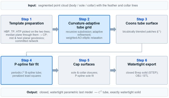
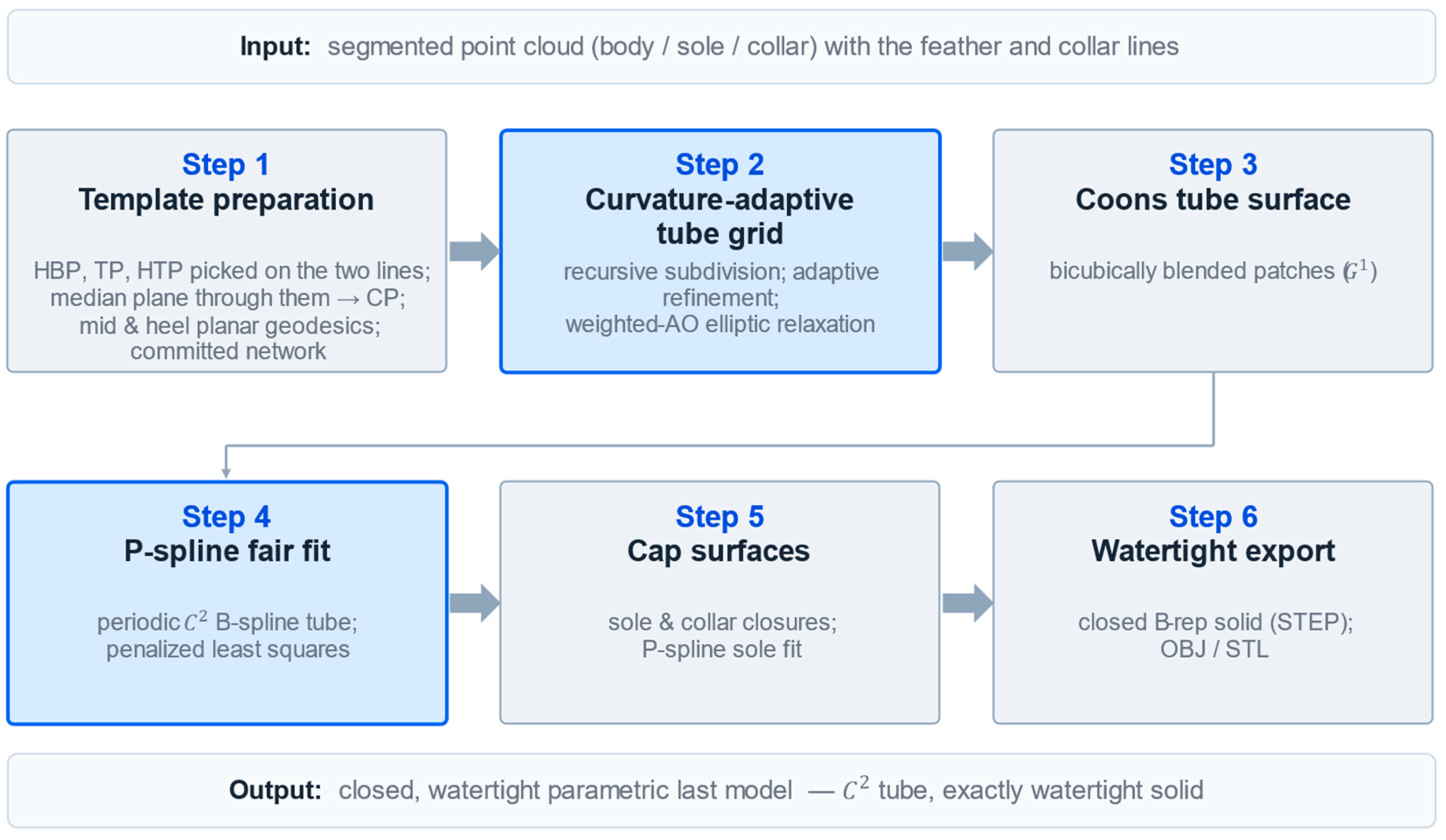
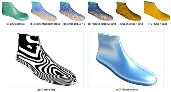
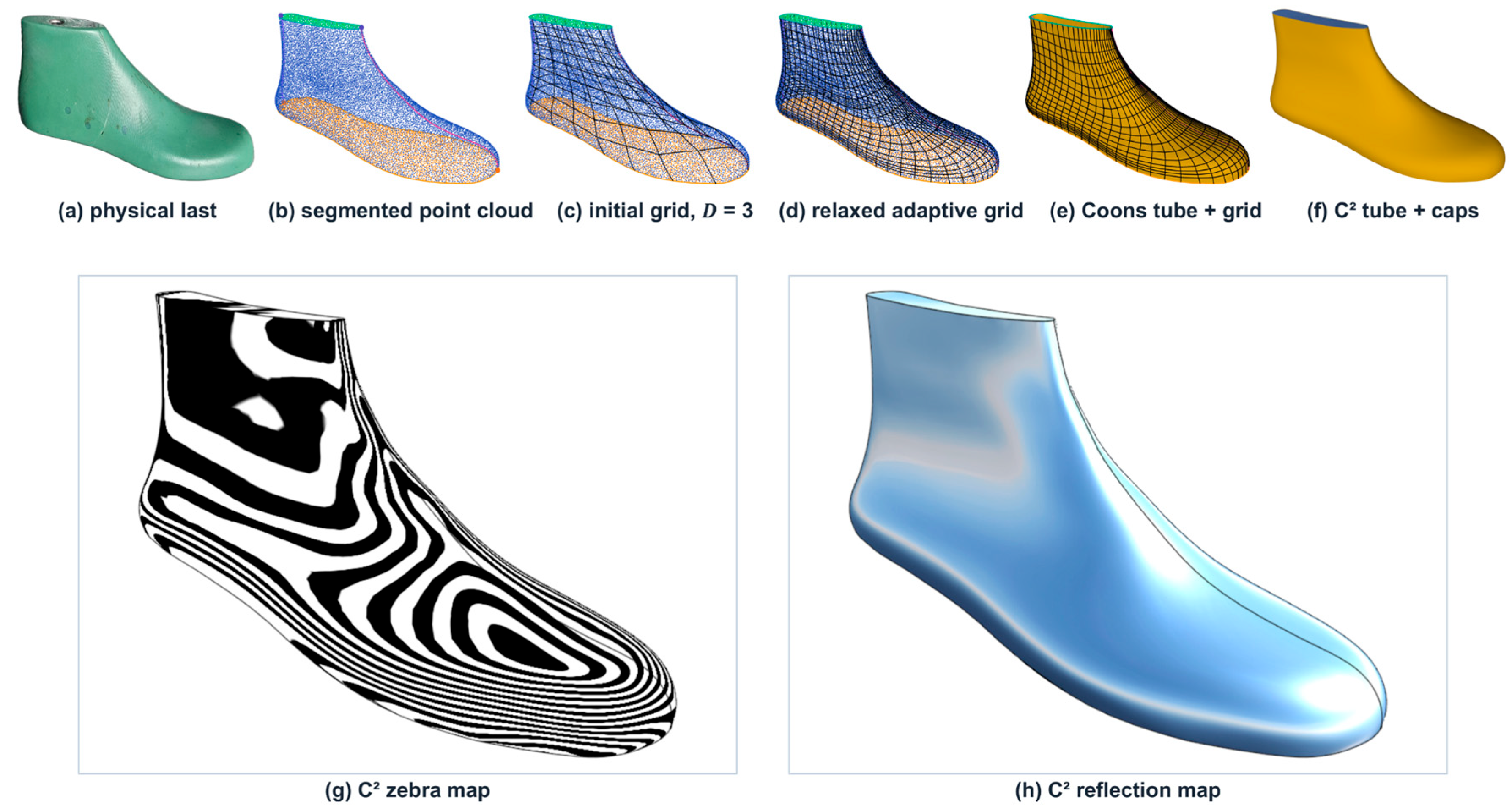
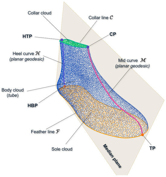
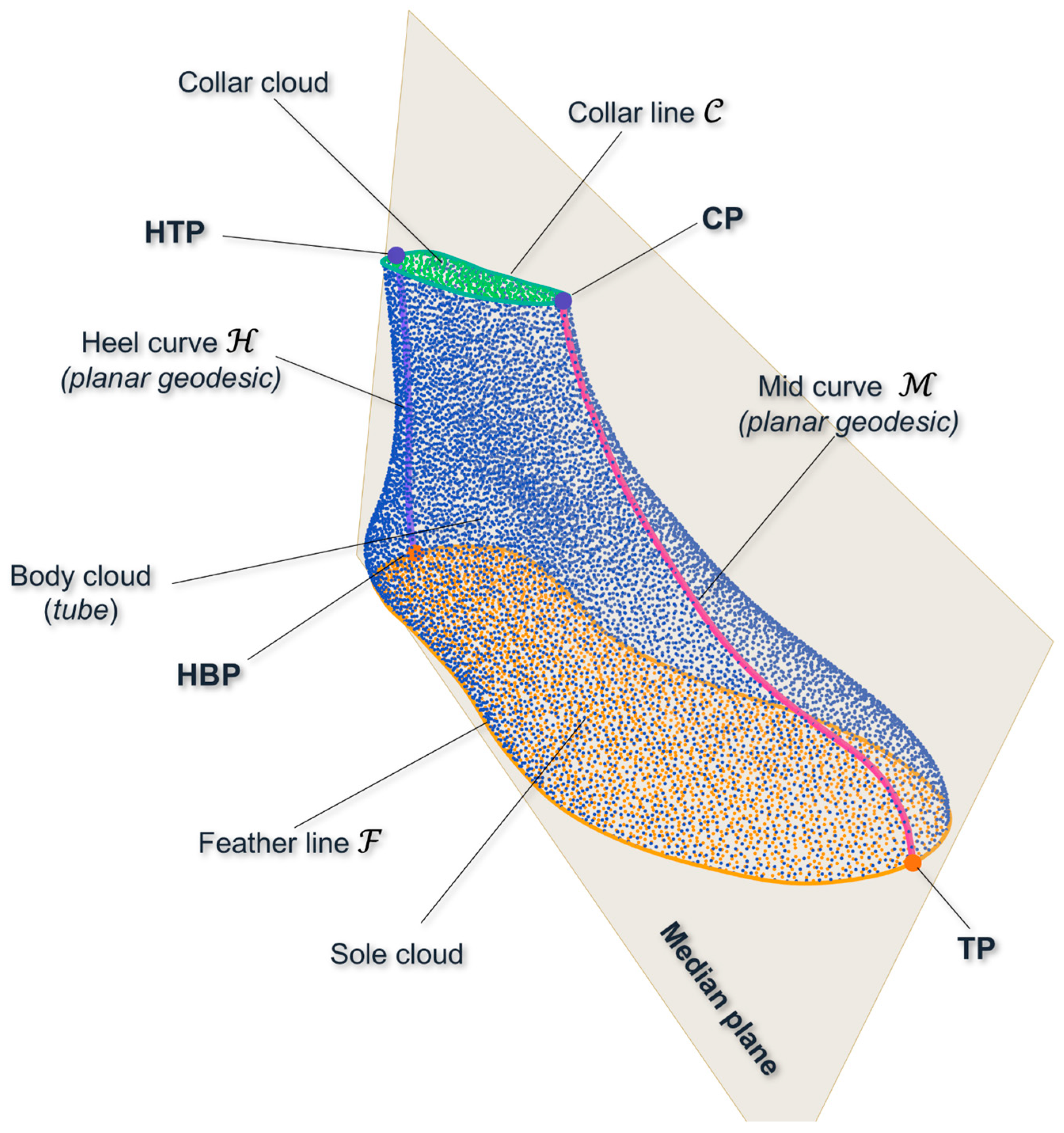
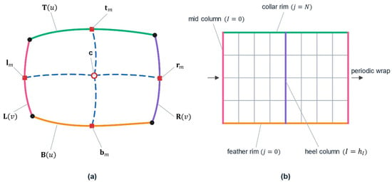
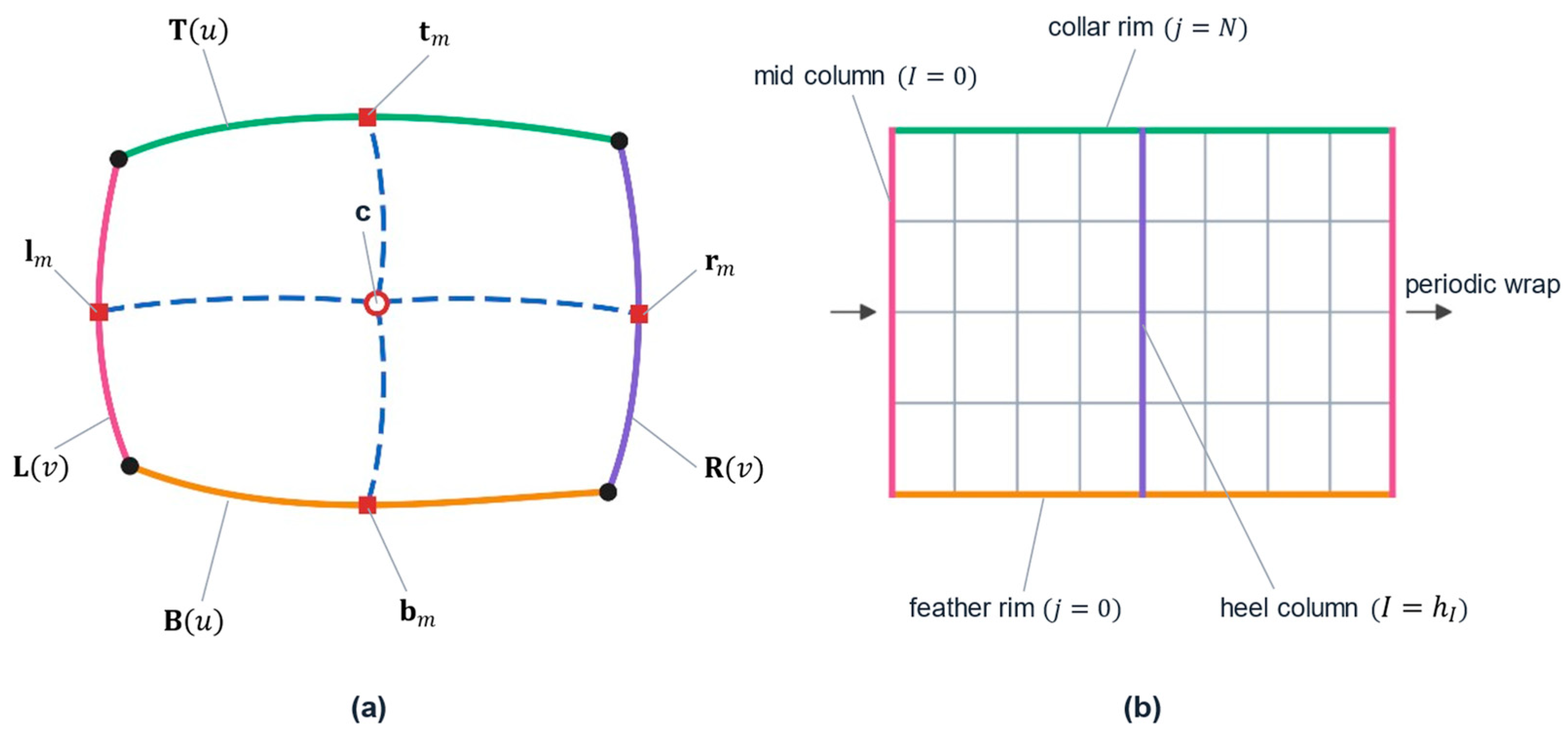
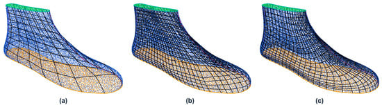
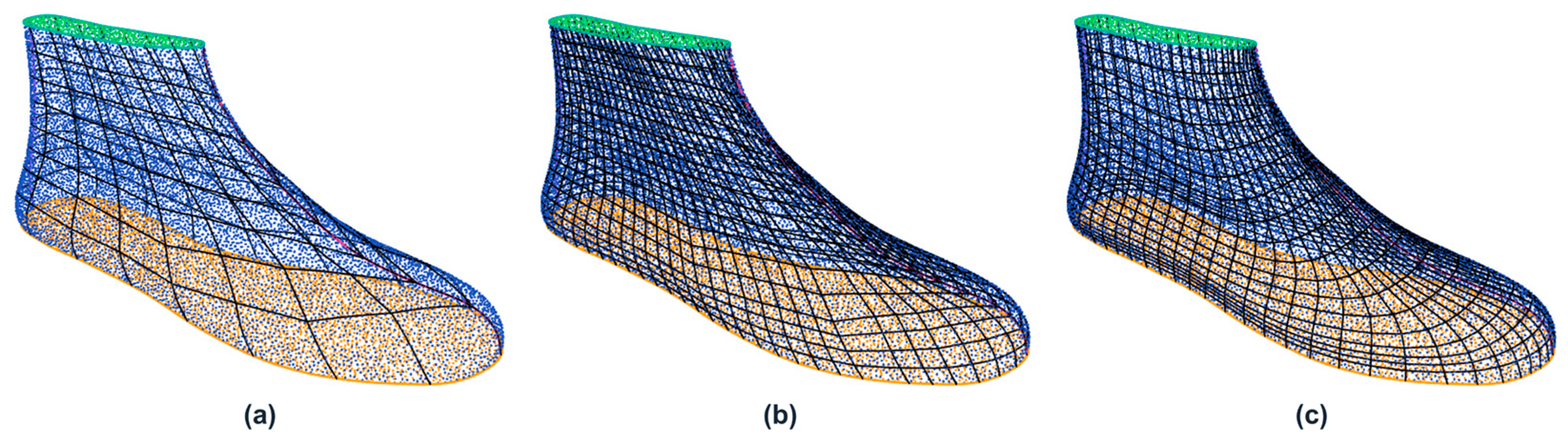
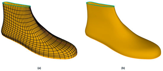
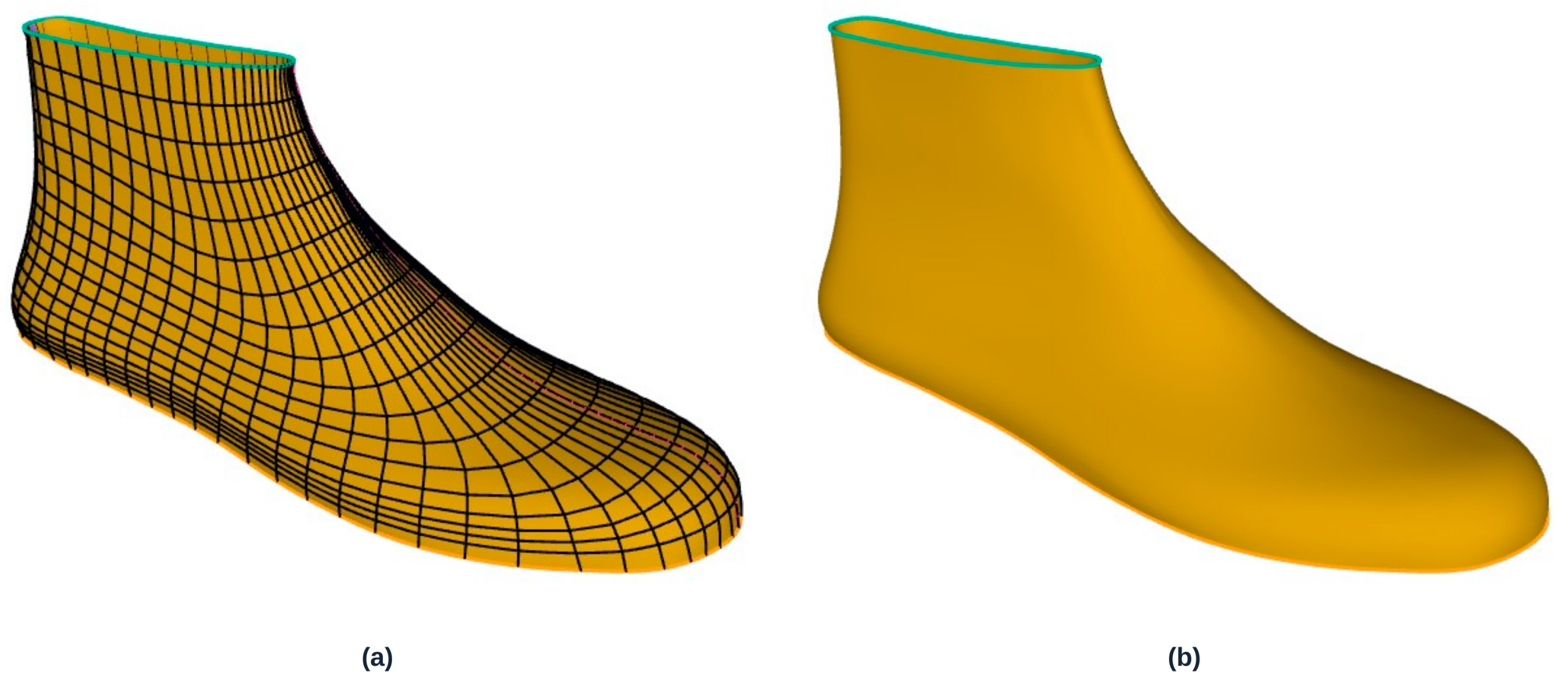
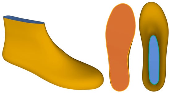
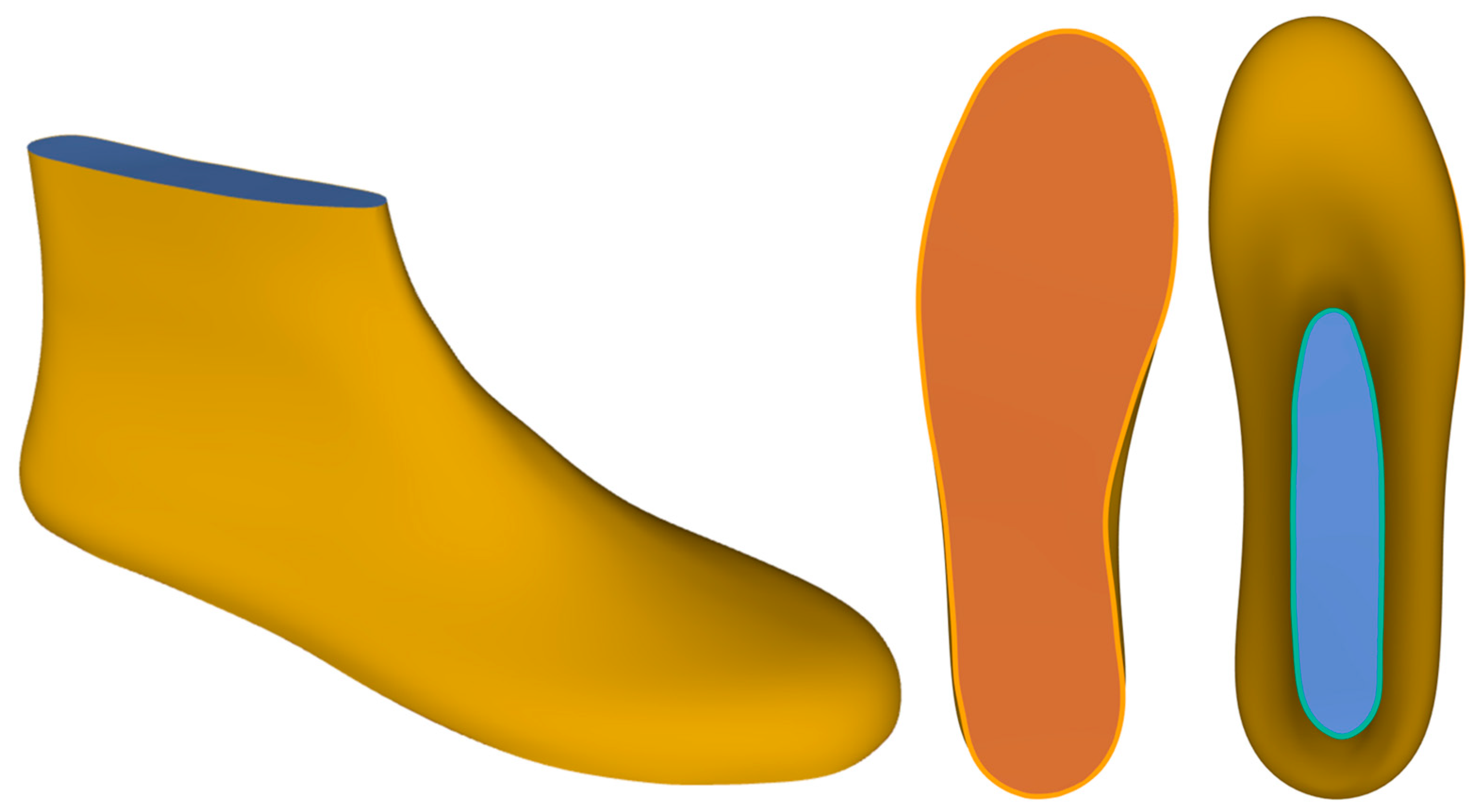
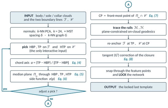
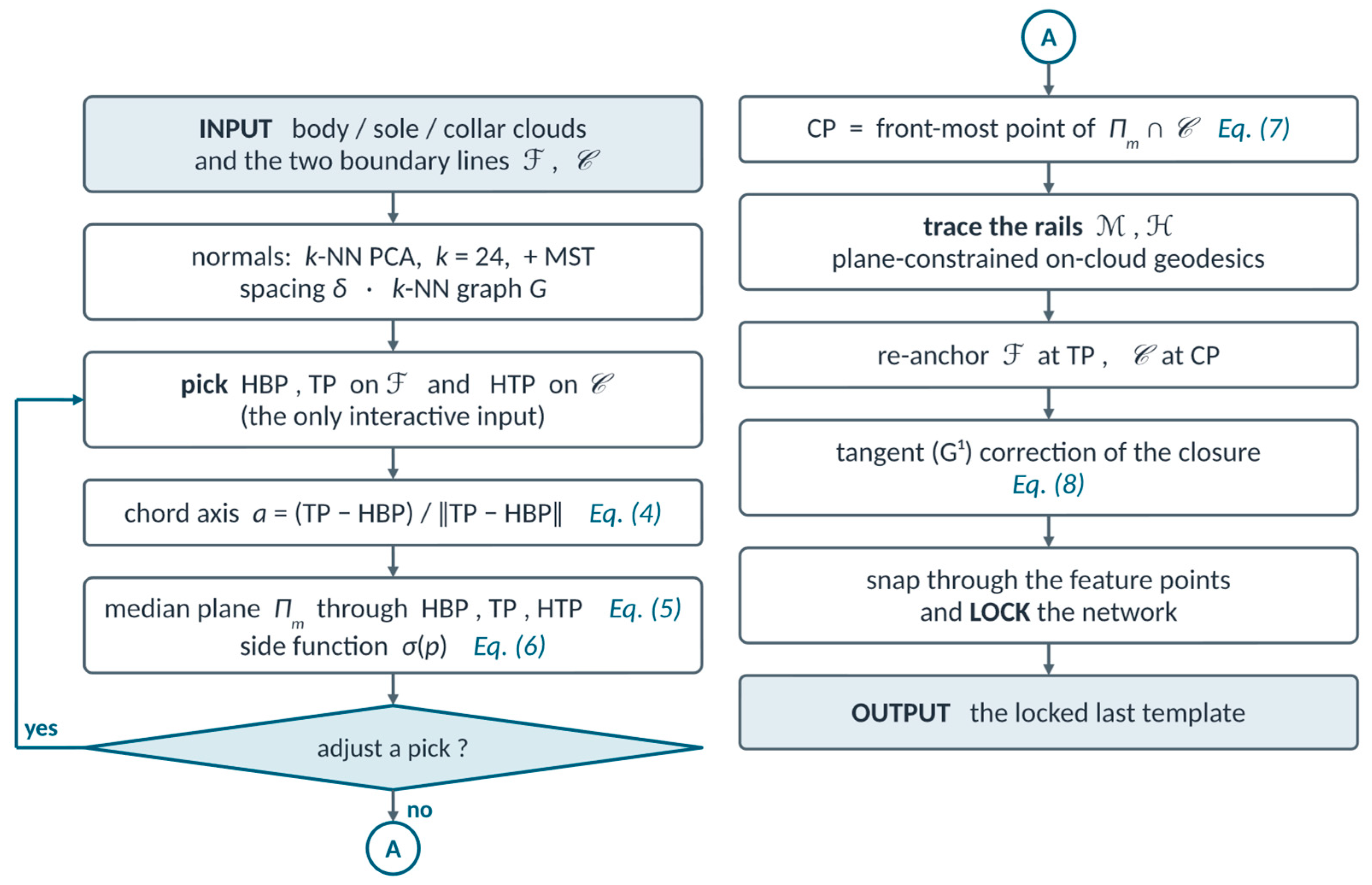
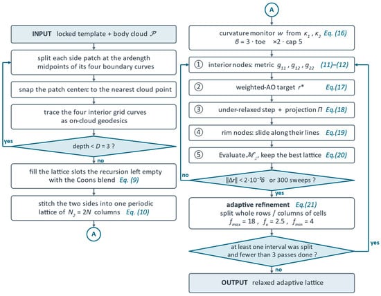
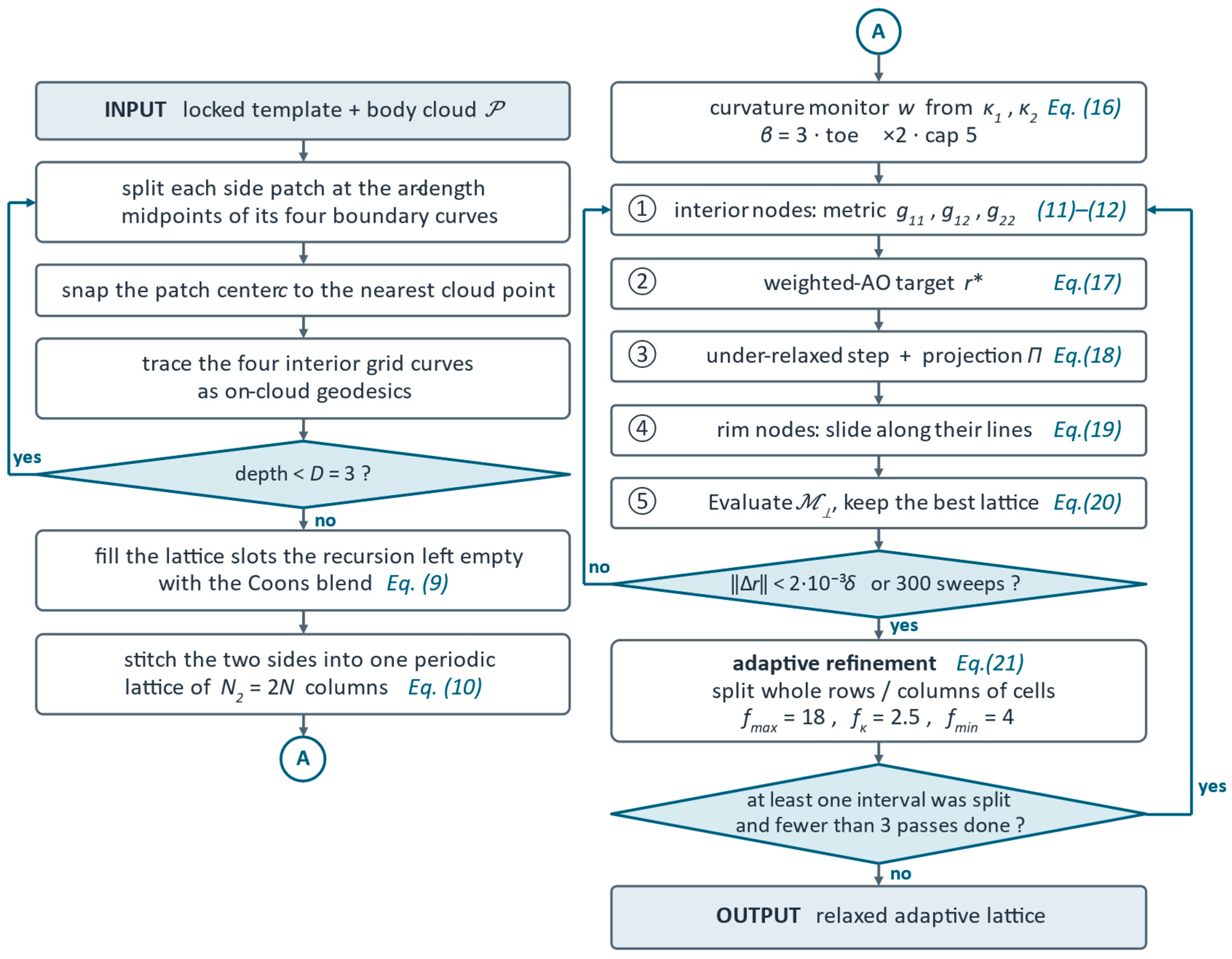
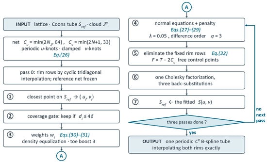
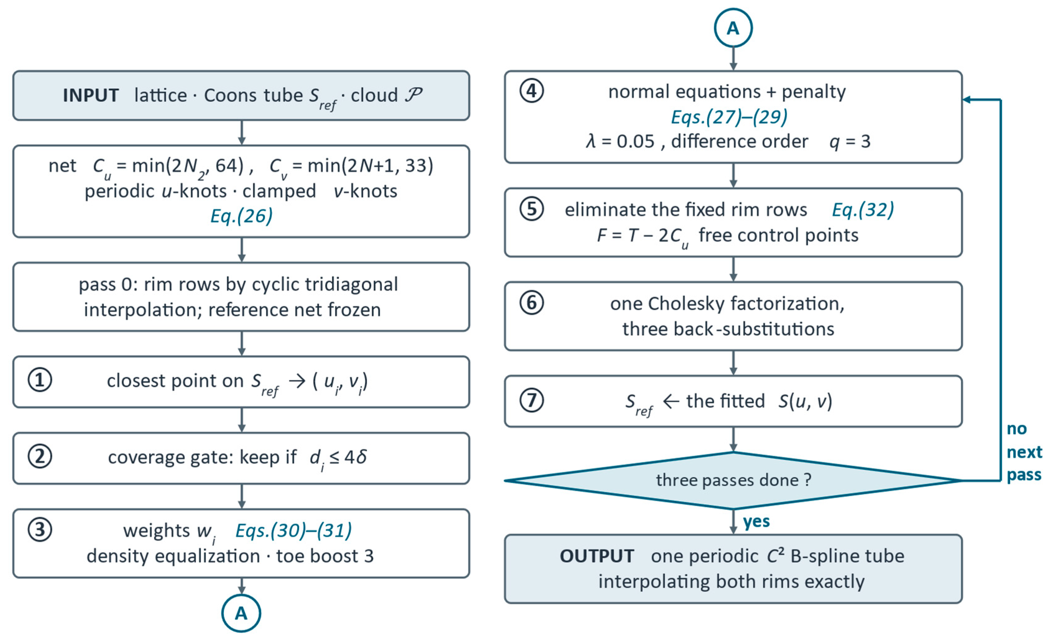
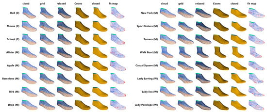
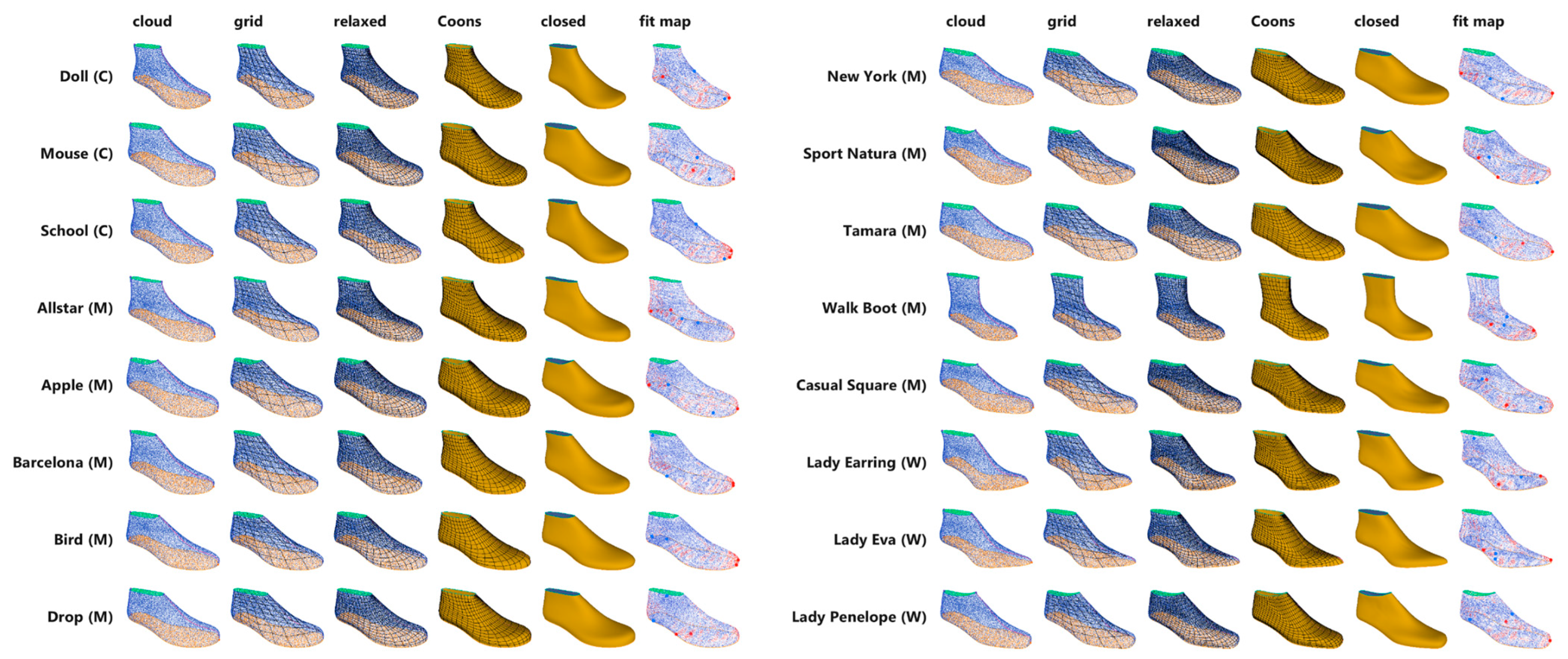
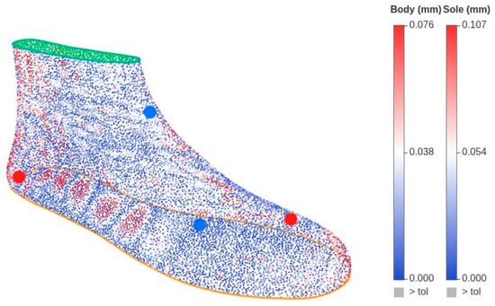
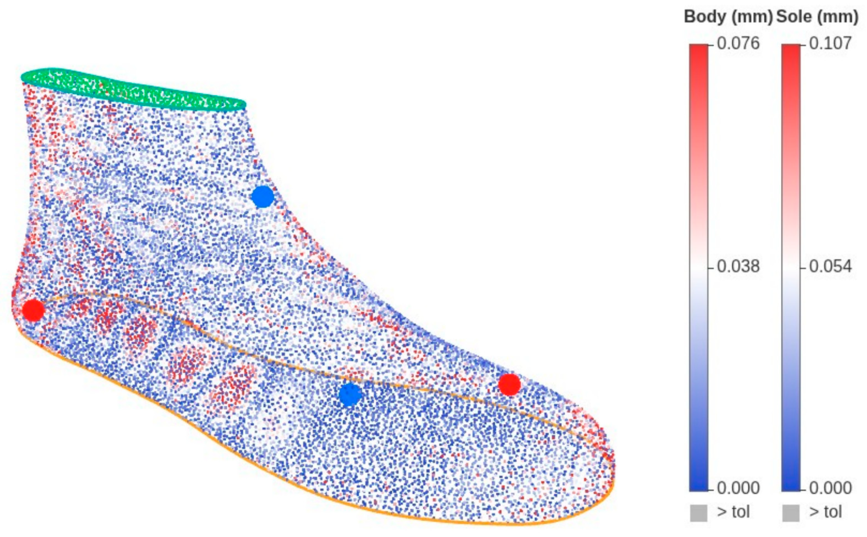
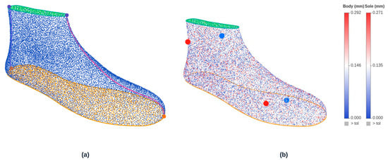
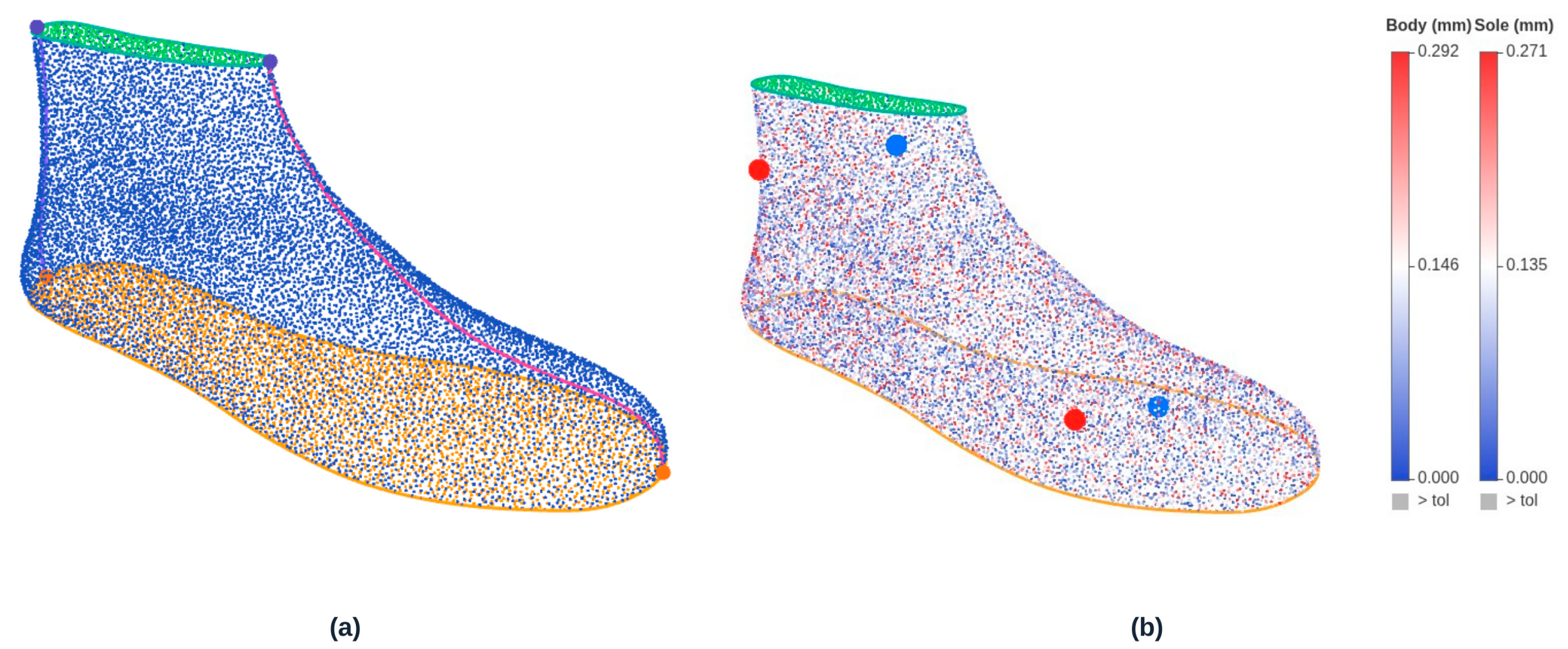
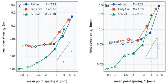
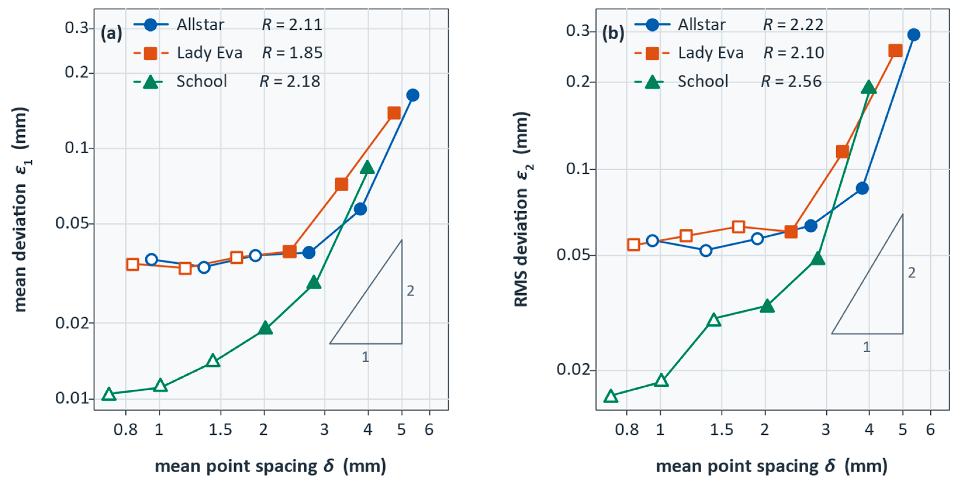
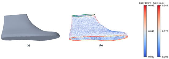
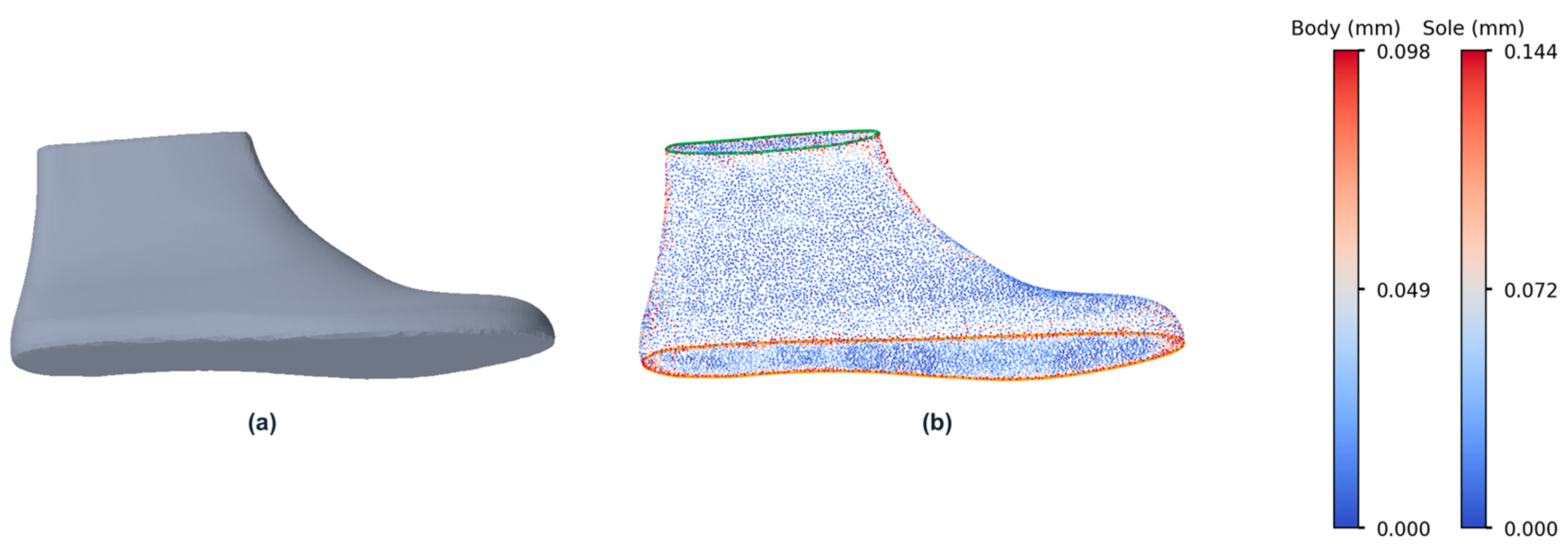
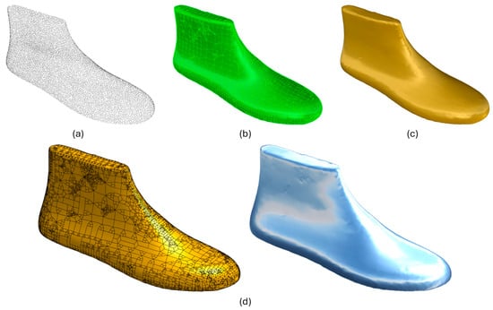
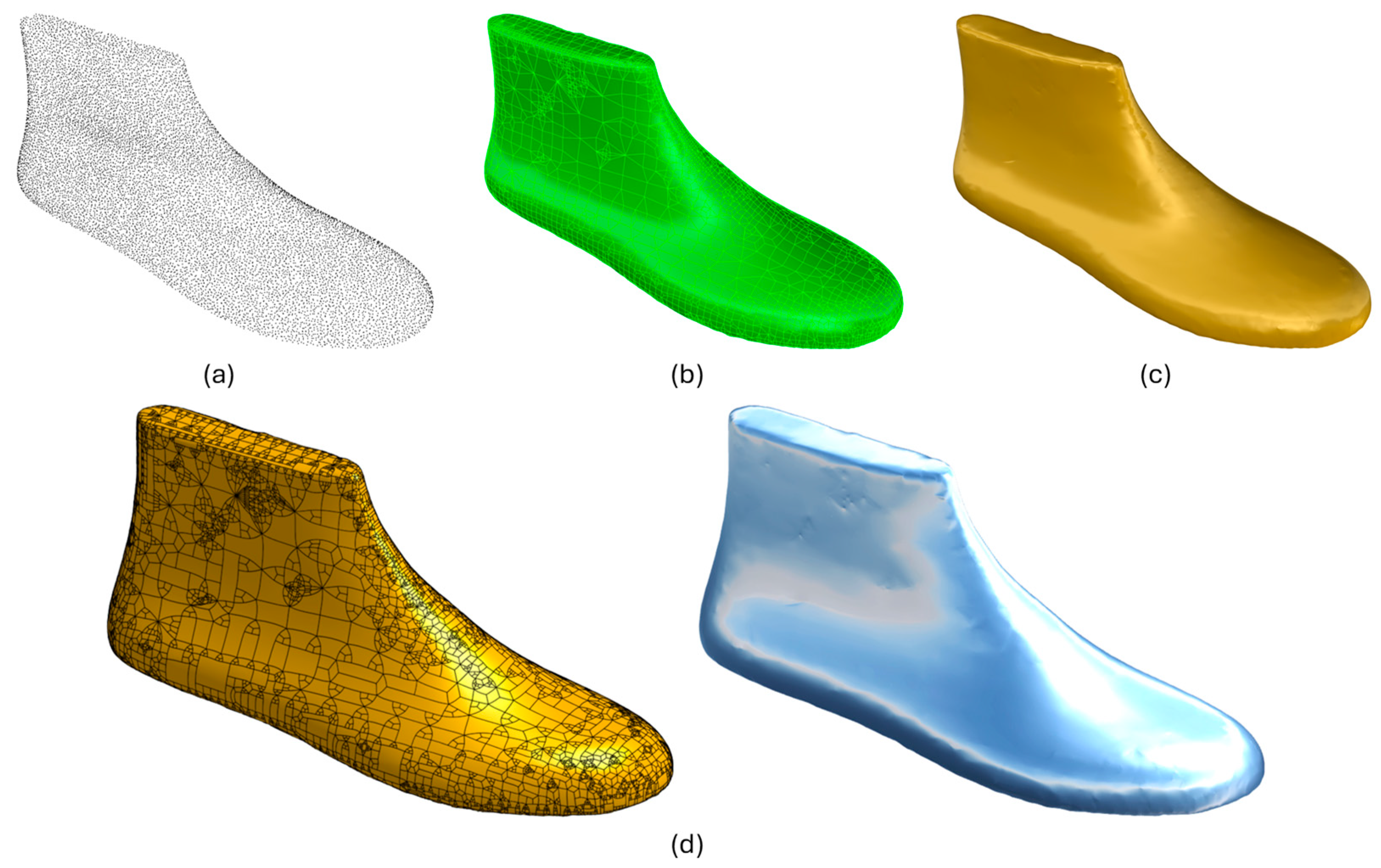

Disclaimer/Publisher’s Note: The statements, opinions and data contained in all publications are solely those of the individual author(s) and contributor(s) and not of MDPI and/or the editor(s). MDPI and/or the editor(s) disclaim responsibility for any injury to people or property resulting from any ideas, methods, instructions or products referred to in the content. |
© 2026 by the author. Licensee MDPI, Basel, Switzerland. This article is an open access article distributed under the terms and conditions of the Creative Commons Attribution (CC BY) license.