


Abstract
Machine learning models offer high discriminatory power for cross-sectional stroke-status classification, yet high-performing models often remain “black boxes” with little intrinsic interpretability. Bayesian networks (BNs) are probabilistic graphical models that offer intrinsic, auditable interpretability without the need for post hoc explanation. We specify a conditional Gaussian Bayesian network over eleven clinical variables, learned by constrained hill-climbing under epidemiologically derived arc constraints, parameterized by Bayesian estimation for discrete nodes and linear Gaussian regression for continuous ones, and queried for posterior stroke probability by Monte Carlo likelihood weighting. Using a 2 × 2 × 2 factorial design on 5109 patients, we crossed three preprocessing decisions—discretized versus continuous topology, median versus single imputation by chained equations (SICE), and no balancing versus synthetic oversampling (SMOTE)—yielding eight configurations, each assessed for discrimination, for calibration against a prevalence-only reference, and across 30 repeated stratified resamples of the entire pipeline analyzed by linear mixed model. Topology was the decisive choice: continuous nodes raised AUC by 0.050 (95% CI 0.038–0.063, p = 2.5 × 10⁻⁹), whereas imputation choice had no detectable effect (p = 0.741). Synthetic oversampling degraded discrimination and interacted antagonistically with topology, harming continuous networks five to six times more than discretized ones (p < 0.001). No configuration exceeded the prevalence-only reference in Brier skill score; a prior correction largely repaired the calibration intercept (−3.01 to −0.04) but not the slope or discrimination loss. The selected network (test AUC 0.811, 95% CI 0.761–0.853) showed no detected difference from logistic regression (AUC 0.819, p = 0.46) or XGBoost (AUC 0.822, p = 0.31). In conclusion, intrinsically interpretable Bayesian networks carried no measured accuracy penalty, though probability estimates require recalibration and longitudinal cohort validation.
1. Introduction
Stroke is a leading cause of death and disability in Canada and worldwide [1]. It has been estimated that up to 80% of strokes are preventable through timely identification and targeted screening of risk factors, including hypertension, smoking, diabetes, and other vascular risks [2]. In the United States, stroke mortality has declined by more than 70% over the past 50 years through advancements in prevention, acute care, and secondary risk reduction [2]. However, substantial disparities persist globally, which drive uneven access to screening, timely care, and health education [3]. For example, approximately 40% of patients presenting to emergency departments with acute stroke are unaware of warning signs and etiological risk factors [4].
Stroke is broadly categorized into two main pathological subtypes: (1) ischemic stroke, caused by occlusion or narrowing of an artery supplying blood to the brain, and (2) hemorrhagic stroke, caused by rupture of a cerebral vessel with intracranial bleeding. Ischemic stroke accounts for roughly 62–71% of incident strokes [5]. While both subtypes present as acute focal neurological deficits, their global burden and demographic distribution are changing rapidly. According to Global Burden of Disease data, although age-standardized stroke mortality rates have steadily declined over recent decades due to improvements in acute care and primary prevention, the absolute global incidence, prevalence, and disability-adjusted life years (DALYs) continue to rise substantially [5]. Moreover, stroke demographics are shifting toward younger populations, with increasing incidence among adults under 55 years driven by the surging global prevalence of metabolic risk factors [5].
At the physiological level, stroke is the acute outcome of progressive vascular degradation, where sustained hemodynamic stress and metabolic toxicity drive endothelial injury (damage to vessel lining), arterial atherosclerosis (fatty plaque vessel buildup), or microvascular rupture (small blood vessel breakage). These pathological cascades are predominantly initiated and accelerated by a core set of clinical and social drivers. The landmark INTERSTROKE study established that modifiable risk factors—dominated by hypertension, cardiac history, elevated BMI, glucose levels, and smoking status—collectively account for approximately 90% of the population-attributable risk for stroke globally [6]. Furthermore, Reshetnyak et al. demonstrated that cumulative sociodemographic factors also serve as significant, independent predictors of incident stroke [7]. Grounding predictive models in these established physiological mechanisms ensures that data-driven features directly reflect the underlying biological etiology of cerebrovascular disease.
Translating these biological risk factors into actionable clinical tools has driven a progression from classical statistical models towards machine learning. Logistic and Cox regression remain the reference standard for clinical risk prediction because they are intrinsically interpretable: a clinician can trace how each risk factor contributes to an individual estimate [8]. As the availability of high-resolution electronic health records has grown, more flexible algorithms have been adopted to capture the nonlinear interactions among vascular and metabolic risk factors [9,10]. These models obscure the transparency of the underlying mathematical models, formalizing a tension in the explainable artificial intelligence (XAI) literature as the interpretability–performance trade-off [11,12]. The schematic architecture of these models is shown in Supplementary Materials, Figure S1.
Stroke prediction has become a proving ground for XAI methods, and two distinct strategies dominate the recent literature. The first strategy pair is a high-capacity opaque model with post hoc explanation. In this paradigm, complex ensemble architectures such as extreme gradient boosting (XGBoost), Random Forests, and Multi-Layer Perceptron (MLP) are deployed to capture complex, non-linear interactions, after which post hoc frameworks like Shapley Additive explanations (SHAP) [13] retrofit feature-attribution metrics to highlight key risk drivers such as age, hypertension, and average blood glucose levels [13,14,15]. Conversely, the second strategy prioritizes intrinsic interpretability by constructing inherently transparent “glass-box” models—such as Bayesian Rule Lists, decision lists, and parsimonious linear or probabilistic models [16,17]. These models are human-readable and significantly outperformed currently established clinical risk scores like CHA2DS2-VASc while maintaining complete decision transparency [16,17].
While these transparent architectures ensure clinical accountability, their intrinsic interpretability frequently comes at the expense of predictive accuracy [18]. Although these models may perform optimally within highly structured and well-defined datasets, they lack the mathematical flexibility required to map the widespread, nonlinear dependencies inherent in real-world clinical data [11]. Consequently, developing targeted diagnostic tools requires navigating a trade-off between maximizing performance and preserving structural transparency, as illustrated in Supplementary Materials, Figure S2.
In the most directly relevant benchmark, Lolak et al. [19] evaluated logistic regression, Cox proportional hazard, Bayesian network, tree-augmented naïve Bayes (TAN), extreme gradient boosting (XGBoost), and explainable boosting machine (EBM) in 275,247 high-risk patients with discretized risk factors, including demographic, cardiovascular, and metabolic variables and medication use. Among these patients, 9659 (3.5%) experienced strokes. The C-statistics of XGBoost, EBM, TAN, logistic regression, and the Bayesian network were 0.89, 0.87, 0.83, 0.80, and 0.80, respectively, so the gradient-boosted ensemble exceeded the interpretable Bayesian network by roughly 0.09 while requiring post hoc analysis to be explained at all [19]. This pattern is consistent with the broader finding that tree ensembles outperform deep networks on tabular data but by margins that narrow as the feature set becomes clinically curated [20,21].
Three gaps are apparent across this literature. First, discrimination is almost universally the sole reported criterion; probability calibration—whether a stated 20% risk corresponds to a 20% observed event rate—is rarely assessed, despite being the property on which individualized clinical decisions actually depend [22]. Second, post hoc attribution explains a prediction after the fact but does not make the underlying model auditable, a distinction Rudin argues is decisive in high-stakes settings [12]. Third, and most relevant here, where intrinsically interpretable models are used, they are typically fitted once, with the preprocessing pipeline treated as an incidental implementation detail rather than as a determinant of performance.
To bridge the gap between predictive performance and model interpretability, Bayesian networks (BNs) present a parsimonious alternative. On the accuracy—interpretability continuum, BNs occupy a strategic intermediate position that bridges simpler transparent models and high-performing opaque architectures. The mathematical foundation of a Bayesian network (BN) is Bayes’ theorem, which provides a rigorous framework for updating the probability of a clinical hypothesis (, such as a stroke diagnosis) on the basis of observed evidence (, such as specific patient risk factors):
where the term represents the posterior probability, which is the probability of the hypothesis given the evidence. In a clinical context, this allows for dynamic risk assessment where the prior probability , which is based on population prevalence, is redefined into a personalized risk score as individual patient data are integrated.
A Bayesian network extends this principle into a probabilistic graphical model that represents the joint probability distribution of a complex set of clinical variables, decomposing high-dimensional data into a product of local conditional distributions via the following theorem:
where represents the joint probability distribution over the entire set of n clinical variables (nodes) in the network, represents the i-th individual random variable (node) in the model, and represents the set of direct parent nodes of variable Xi in the directed acyclic graph (DAG).
The conditional probability table (CPT) serves as the primary parameterization of the network. Each CPT quantifies the probabilistic relationship between a “child” node and its “parent” nodes by explicitly listing the probability of every possible child state given all combinations of parent states. For example, a CPT for the node “Stroke” calculates specific risk probabilities on the basis of discrete parent states such as “Old Age” and “High Glucose”. This modular structure ensures that the model remains decomposable, as individual tables can be isolated and audited by clinicians to verify that the algorithmic logic remains biologically plausible and aligned with clinical domain expertise.
Bayesian networks have been implemented in disease diagnosis and risk prediction, including for cardiovascular disease [23], atrial fibrillation relapse [24], and ALS diagnosis [25]. Suo et al. [26] developed a BN-based model using EHR data from 169,692 patients in Chinese hospitals to predict 3-year CHD risk. A weighted survival Bayesian network was developed by combining inverse probability censoring weights and a Cox model using demographic, laboratory, and medical history variables as risk factors. The model achieved an AUC of 0.80 despite extensive missing data and imbalanced datasets. Similarly, Park et al. [27] applied a BN to predict 3-month functional outcomes (mRS) and 1-year mortality in 2432 ischemic stroke patients using 74 features (risk factors), including baseline NIHSS scores and age, attaining an AUC of 0.89 for 3-month functional outcomes and 0.89 for 1-year mortality. They also developed a Yonsei outcome inference system via their trained model.
Arrieta et al. identify two research trajectories for reconciling accuracy with transparency: applying post hoc explanation to opaque models or improving the performance of intrinsically interpretable models through better model construction and data preparation [11]. We pursue the second. This choice is deliberate: post hoc explanation leaves the underlying model un-auditable and, as Rudin argues, substitutes an approximation of the reasoning for the reasoning itself [12]. If the discrimination gap for BNs is attributable to preprocessing rather than to representational capacity, then it should be closable without comprising interpretability—and that proposition is testable.
We therefore examine the three preprocessing decisions that the literature identifies as most consequential for probabilistic graphical models on clinical data, each selected for a specific reason rather than by convenience. (i) Variable topology. Standard BN implementations require discrete variables, so continuous physiological measurements are conventionally binned into clinical categories. Discretization is known to discard information and to reduce predictive performance in regression settings [8], and hybrid conditional Gaussian networks permit continuous variables to be retained with a Gaussian local parameterization [28]. Whether this theoretical advantage translates into measurable gain in a clinical BN has not been established. (ii) Missing-data handling. Physiological variables are frequently incomplete, and imputation by chained equations is widely recommended over simple substitution in the machine learning literature [9,10]—including in the largest BN stroke study to date [19]—yet a generative model that represents the full joint distribution may be less sensitive to the imputation method than a discriminative one. (iii) Class imbalance. Stroke prevalence in screening cohorts is low, and synthetic minority oversampling is routinely applied to force recognition of the minority class [29,30]. However, oversampling alters the outcome prior, and recent work in clinical prediction shows that imbalance correction degrades probability calibration without improving discrimination [31]. For a model whose clinical value resides in its probabilities, this trade-off is decisive and requires direct examination.
The aim of this study is therefore to determine which preprocessing decisions govern the performance of a hybrid Bayesian network for stroke likelihood estimation, and whether an interpretable model so configured can match opaque benchmarks on both discrimination and calibration. Rather than reporting a single tuned model, we adopt a factorial design that varies the three decisions above simultaneously, so that the independent contribution of each—and any interaction between them—can be estimated. Model quality is judged on discrimination and on calibration jointly, because a model that ranks patients well but misstates their absolute risk is not usable for individual decisions.
We present a rigorous, eight-arm methodological study evaluating the predictive architecture of Bayesian networks. We systematically isolate the effects of network topology (purely discretized vs. hybrid continuous nodes), imputation strategies (baseline median imputation vs. single imputation by chained equations [SICE]), and class balancing (unadjusted vs. synthetic minority oversampling technique [SMOTE]).
By isolating the effect of each methodological variation, we formulated the hypothesis shown in Table 1.
Table 1.
Null and alternate hypotheses for each preprocessing factor.
2. Materials and Methods
2.1. Problem Formulation and Notation
We treat stroke risk estimation as a cross-sectional probability classification problem. Let X = (X1, …, X10) denote the vector of recorded clinical variables for a patient—demographic, medical history, physiological, and lifestyle—and let S ∈ {0, 1} denote recorded stroke status. The quantity to be estimated is the conditional probability together with the conditional independence structure that generates it, so that the contribution of each variable can be audited rather than attributed after the fact.
Two properties of the data determine what this quantity can represent, and they constrain the modeling choices that follow. First, the cohort is cross-sectional: risk factors and stroke status are recorded contemporaneously, with no event dates, no follow-up interval, and no observed ordering between exposure and outcome. Equation (3) therefore describes how estimated risk differs between patient profiles within a population; it is not a transition between an earlier and a later state, and no time-to-event quantity is identifiable from these data. Second, and consequently, r(x) is an observational conditional probability and is not in general equal to the interventional quantity P(S = 1|do(X = x)) that a claim about modifying a risk factor would require [32]. The Bayesian network formalism is not itself restricted in this way—a dynamic Bayesian network extends the same factorization across time slices and expresses exactly the transition model that longitudinal records would support—but that extension requires data this cohort does not contain.
The task addressed in this study is accordingly the estimation and audit of Equation (3) under eight alternative data-preparation techniques, and the identification of which of those techniques govern its accuracy and its reliability as a probability.
2.2. Bayesian Network Specification
The networks fitted here are Bayesian networks in the sense of Equations (1) and (2): a directed acyclic graph G = (V, A) whose nodes are the eleven clinical variables and whose arcs encode direct probabilistic dependence, with the joint distribution factorized into one local conditional distribution per node. For a discrete node the local term is a conditional probability table; for the continuous arms of this study the network is a conditional Gaussian Bayesian network (CG-BN) [28].
A CG-BN treats discrete and continuous nodes differently. For a continuous node Y, the local distribution is a linear regression on Y’s continuous parents. This regression is fitted separately for each combination of Y’s discrete parents:
Y | (I = i, Z = z) ~ N(μi + βiTz, σi2)
Here i indexes one combination of Y’s discrete parent states; μi and βi are the intercept and slope of the regression for that combination; σi2 is its residual variance. In words: each discrete-parent combination gets its own regression line for Y.
This is why topology matters. A discretized network places a 60-year-old and a 65-year-old in the same age band and treats them identically. A continuous network estimates a separate mean and variance for each, so risk varies smoothly with the exact value rather than jumping at a bin boundary. This difference underlies the discrimination gain reported in Section 3.3.
One structural constraint follows from Equation (4). A continuous node cannot be the parent of a discrete node. Arcs between a discrete node and a continuous node can therefore point only one way: away from the discrete node. Stroke is discrete; age and glucose are continuous. Any arc between them must point away from stroke, regardless of what the data show. This is a property of the representation, not a finding. Its consequences for interpretation are examined in Section 3.6 and Section 4.6. The whitelists and blacklists used to enforce admissible structures in each arm are given in Section 2.7.
2.3. Analysis Pipeline
To systematically evaluate cross-sectional stroke-probability estimation while maintaining intrinsic probabilistic interpretability, we developed a structured, end-to-end machine learning framework. The core methodology encompasses stratified data partitioning, controlled preprocessing, constraint-based structure learning, parameter estimation, probabilistic inference, and rigorous validation-based evaluation. The overall pipeline is summarized in Algorithm 1.
| Algorithm 1: End-to-end pipeline for conditional stroke-probability estimation, showing the fixed processing stages and the three experimental decision points. |
| Input: Raw patient records (demographics, medical history, lifestyle factors, and stroke outcomes) Outcome: Trained conditional stroke-probability model, optimal risk cutoff threshold, out-of-sample performance metrics Stage 1: Stratified data splitting (Fixed pipeline); 1. Partition the dataset into training (60%), validation (20%) and test (20%) sets, maintaining the original stroke prevalence rate of 4.87% across all groups; Stage 2: Model training stage (Experimental arms); 2. Missing data imputation: Fill in missing values using either median imputation or single imputation by chained equation (SICE), excluding the stroke outcome during validation and testing imputation; 3. Feature formatting: Retain continuous measurements (such as age and BMI) as numeric values or group them into categories based on WHO guidelines; 4. Class imbalance correction: Address the low proportion of stroke cases in the training set by applying SMOTE or retaining the unbalanced data; 5. Network learning: Learn relationship paths and estimate conditional probabilities using search algorithms guided by clinical rules to build the trained model; Stage 3: Inference and model evaluation stage; 6. Transform evaluation sets: Applying the missing-value filling rules and feature definitions learned during training to the validation and testing sets; 7. Calculate risk probabilities: Generate posterior stroke risk probabilities for validation and test patients using Monte Carlo likelihood weighting simulations (1000 particles); 8. Threshold optimization: Determine the optimal decision cutoff on the validation set using Youden’s J statistic to balance true stroke detection against false alarms; 9. Final performance evaluation: Apply the chosen threshold to the held-out test set to calculate AUC, Brier score, Brier Skill Score (BSS), validation threshold, sensitivity and specificity. |
Each stage draws on an established method rather than a new one. Stratified partitioning before any preprocessing follows standard guidance for avoiding information leakage in clinical prediction and stratification modeling [8]. Structure learning uses score-based hill-climbing, constrained by whitelists and blacklists derived from epidemiology and temporal ordering [1,6], and parameter estimation combines Bayesian estimation with a Dirichlet prior for discrete nodes and the conditional linear Gaussian form of Equation (4) for continuous ones [28]. Chained-equation imputation was used in preference to simple substitution because it preserves the joint distribution among the predictor variables during the missing-data fill, and class imbalance is corrected by SMOTE [29], with threshold selection by the Youden index [33]. Inference throughout uses Monte Carlo likelihood weighting, specified in Section 2.9. The three decision points in Stage 2—imputation, feature representation and balancing—are the three factors varied across the eight study arms; every other step is held fixed.
2.4. Overview of the Dataset and Partitioning
We utilized an open-source Stroke prediction dataset, which is available at Kaggle [34]. The dataset has been widely adopted in machine learning research, with approximately more than 275,000 downloads, and is used in 103 research articles [35]. Ethical approval and informed consent were not required for this study.
The dataset consists of 10 features along with the diagnosis of stroke. The raw data file contains 5110 records—4861 non-stroke and 249 strokes. One patient recorded with an indeterminate sex category was excluded, giving an analysis cohort of 5109 patients: 4860 non-stroke and 249 strokes, a stroke prevalence of 4.87%. The cohort is therefore strongly imbalanced. The summary of the features is shown in Supplementary Materials, Table S1.
To prevent information leakage, the data underwent a strict, stratified training-validation-test (60-20-20) split prior to any preprocessing. This preserved the baseline 4.87% prevalence across all subsets:
- Training set: n = 3065 (149 stroke cases)
- Validation set: n = 1022 (50 stroke cases)
- Test set: n = 1022 (50 stroke cases)
The dataset features incorporate continuous, binary, and categorical values. These features are broadly categorized into the following aspects:
- Sociodemographic: age, sex, residence type, marital status, and occupation
- Medical history: Hypertension and heart disease
- Physiological measurements: BMI (body mass index) and average glucose level
- Lifestyle factor: Smoking status
2.5. Preprocessing and Imputation Strategies
Continuous variables need to be converted to categorical variables for the Bayesian network. Age was categorized on the basis of the WHO’s standard age group (differences of 5 and 85+) [36]. Similarly, body mass index (BMI) has also been categorized on the basis of the WHO [37]: underweight (less than 18.4 kg/m2), normal weight (18.5 to 24.9 kg/m2), overweight (25 to 29.9 kg/m2) and obese (greater than 29.9 kg/m2). Diabetes was classified as present if the average glucose was ≥126 mg/dL, prediabetes if 100–125 mg/dL, and normal if <100 mg/dL [38]. This glucose-only approach ensures consistency in aggregated data while acknowledging limitations such as ignoring timing, symptoms, A1C, medications, and comorbidities that influence accurate diagnosis.
Alternatively, we maintain these variables in their continuous form by employing a hybrid Bayesian network (HBN) structure [28]. To implement this hybrid approach, the following steps were taken:
- Age, BMI, and average glucose were preserved as exact numeric values.
- The conditional distribution of continuous nodes was specified by a Gaussian function via conditional linear Gaussian distributions.
- We utilized structure and parameter learning algorithms explicitly designed for mixed-data networks to estimate outcomes accurately.
Body mass index is the only variable with missing values, absent for 201 of 5109 patients (3.9%). Median substitution replaces each missing value with the median of the observed training values, applied unchanged to the validation and test partitions so that no information crosses the split. Single imputation by chained equations (SICE) instead predicts each missing BMI value from the other recorded variables by predictive mean matching, iterated to convergence over five iterations with a single completed dataset (m = 1); because m = 1, this is single imputation, not pooled multiple imputation, and no between-imputation variance is propagated. The outcome was retained as a predictor when imputing training rows, where it is legitimately observed, and excluded when imputing validation and test rows.
Where balancing was applied, the synthetic minority oversampling technique (SMOTE) [30] was used on the training partition only. For each minority patient, one of its five nearest minority neighbors is selected at random, and a synthetic record is generated as a weighted average of the two—a linear interpolation with the weight drawn uniformly between 0 and 1—repeated until the two classes are equally represented. Because this interpolation acts on raw continuous values, a synthetic value falls into an existing bin in a discretized network but enters the continuous regression of Section 2.2 directly in a conditional Gaussian one; this is the mechanism behind the topology × balancing interaction reported in Section 3.3.
Because oversampling to 50% prevalence alters the outcome prior, probabilities from balanced arms are additionally reported after a prior correction: a constant offset, computed only from the training and target prevalences, is subtracted on the log-odds scale. The correction requires no refitting and no held-out data.
2.6. Study Design and Experimental Arms
This study employs a 2 × 2 × 2 factorial design to evaluate the impact of different data preparation techniques on model performance. Figure 1 illustrates the overall methodological framework, distinguishing between standard pipeline procedures and experimental variables. The baseline methodology (Model M1) establishes a fixed processing pipeline that is applied uniformly across all the models. To prevent data leakage, a standard training-validation-test (60-20-20) split is executed prior to any data manipulation. Following the split, preprocessing choices are applied: median missing value imputation, feature discretization, and no class balancing. The end-to-end analytical workflow, distinguishing fixed pipeline procedures from experimental decision points, is illustrated in Figure 1.
Figure 1.
Experimental workflow.
To evaluate potential improvements over the baseline, three experimental variations were introduced at key methodological decision points (denoted by dashed lines in Figure 1):
- Imputation: Median vs. SICE
- Feature type: Discretized vs. Continuous
- Training Set Balancing: None vs. SMOTE
Standard SMOTE was selected over boundary-focused variants (e.g., Borderline-SMOTE) to address the 4.87% stroke prevalence without over-amplifying noisy or atypical clinical cases near the decision boundary [30]. To counteract the probability miscalibration inherent to synthetic oversampling, decision thresholds were optimized on the validation set using Youden’s J statistic [33].
Based on the permutations of these three variables, the data were processed through eight distinct analytical study arms (Models M1 through M8), as detailed in Table 2. This configuration effectively isolates the individual and combined effects of SICE, continuous features, and SMOTE, allowing for a comprehensive comparison of how each preprocessing variation impacts overall predictive accuracy.
Table 2.
Study design arms 2 × 2 × 2 factors. (Cont. = continuous; SICE = single imputation by chained equations; SMOTE = synthetic minority oversampling technique).
2.7. Structure Learning
The structure of the Bayesian networks (BNs) was learned via the hill-climbing (HC) heuristic search algorithm. Constraints were specified a priori from established epidemiology rather than from any sample association analysis. Arcs from age, hypertension, heart disease, and average glucose to stroke were whitelisted on the basis of the INTERSTROKE population-attributable-risk analysis [6] and the GBD 2021 stroke risk-factor study [1]; arcs into age and sex were blacklisted on temporal grounds.
Different structural constraints were applied depending on whether the experimental arm utilized purely discrete or hybrid (mixed continuous-discrete) data. For hybrid arms, specialized whitelists and blacklists are required to accommodate the mathematical constraints of conditional Gaussian Bayesian networks (CGBNs), which restrict certain topological relationships (e.g., preventing continuous nodes from acting as parents to discrete nodes). To guarantee the robustness of the learned structures and avoid overfitting to the training set, model averaging by bootstrapping was employed. Structural stability was assessed by bootstrap resampling with 200 replicates; the resulting arc strengths are reported as edge-stability diagnostics, and a bootstrap-averaged consensus network was additionally fitted and compared with the single hill-climbing structure.
2.8. Parameter Learning
Following structure learning, conditional probability tables (CPTs) and distributions were estimated from the training data. For purely discrete experimental arms (e.g., M1, M2), parameter learning was conducted via Bayesian estimation. To prevent zero-probability errors for rare feature combinations, an imaginary sample size (ISS) of 10 was applied, effectively acting as a smoothing prior. For hybrid networks containing continuous nodes (e.g., M3, M5), standard maximum likelihood estimation was used to fit the local probability distributions.
2.9. Probabilistic Inference
To generate posterior stroke probabilities across network configurations, Monte Carlo likelihood weighting was consistently applied, as exact inference is computationally intractable for complex hybrid Bayesian networks. Patient-level probability estimation used M = 1000 independent simulations per network to yield stable estimates, whereas population-level conditional-risk queries used logic sampling with M = 106 particles to minimize variance under coarse evidence sets.
Given observed patient evidence E, non-evidence nodes are forward sampled conditionally given their parents, while evidence nodes remain fixed at observed values. Each particle receives a weight equal to the joint likelihood of its observed evidence under that sample’s specific parent configuration. The estimated posterior stroke probability (S = 1) is then computed as the sum of weights for particles yielding a positive stroke outcome divided by the total weight across all M particles.
This formulation transforms the network into an adaptable predictor: because any subset of the eleven clinical variables can serve as evidence E, posterior probabilities can be generated directly for patients with incomplete records without requiring prior data imputation or model retraining.
2.10. Model Evaluation and Statistical Analysis
The operating threshold was selected on the validation set, and the primary model configuration was selected on validation performance alone. The held-out test set was used once. Findings are verified along four independent axes: discrimination is compared between configurations by DeLong’s test for correlated ROC curves on the same test cohort; the contribution of each preprocessing decision is estimated by a linear mixed model fitted to 30 repeated stratified resamples of the entire pipeline; probability calibration is assessed against a prevalence-only reference model; and the selected model is benchmarked against one transparent and one opaque comparator trained on identical partitions. Structural stability is assessed separately by bootstrap resampling of the structure-learning step. Because stroke datasets are inherently imbalanced, a default classification threshold of 0.5 is often suboptimal. Therefore, for each model, a receiver operating characteristic (ROC) curve was generated, and the optimal classification threshold was determined dynamically via the Youden index (Youden’s J statistic) [33]. This method selects the threshold that maximizes the sum of sensitivity and specificity, ensuring a balanced clinical trade-off between identifying true stroke cases and minimizing false alarms.
Using these model-specific thresholds, confusion matrices were constructed for the test set. Per the study design, primary model selection was based on discrimination alone (area under the ROC curve, AUC); calibration was assessed separately, in Section 3.4, and did not enter the selection rule. When evaluating configurations, a parsimony rule of 0.005 was applied: simpler, natively interpretable structures were favored if their discrimination fell within a 0.005 AUC margin of more complex variations
To ensure statistical rigor and evaluate the generalizability of the findings, the entire pipeline was harmonized across 30 stratified resamples. The eight pipeline arms representing the 2 × 2 × 2 factorial designs (topology × imputation × balancing) were evaluated across these 30 iterations using a linear mixed model (LMM). By setting the resample seed as a random intercept, we extracted Type III tests of fixed effects to determine whether the effects of the combined strategies were additive or interacting. Because the 30 resamples are drawn from a single cohort and therefore share observations, inference from this model is conditional on this dataset; a Nadeau–Bengio variance correction for repeated random subsampling is reported as a sensitivity analysis.
Pairwise differences were tested with DeLong’s test for correlated ROC curves (AUC) and McNemar’s test on the true-positive cohort (sensitivity). Furthermore, paired t-tests and Wilcoxon signed-rank tests were utilized to directly compare the per-seed AUC distributions between the continuous (hybrid) and discrete baseline topological arms. Because rare outcomes can create sparse conditional probability table (CPT) configurations, CPT reliability was formally evaluated using exact Jeffreys credible intervals for specific target cells, supplemented by an imaginary sample size (ISS) sensitivity analysis to measure parameter shrinkage toward marginal probabilities under increasing prior strength. The underlying structural stability of the learned graphs was verified by extracting a bootstrap-averaged consensus network.
Finally, logistic regression and an early-stopped gradient-boosted ensemble (XGBoost) were trained on identical splits to serve as fully transparent and high-capacity opaque benchmarks. The gradient-boosted ensemble used a binary logistic objective with maximum tree depth 3, learning rate 0.05, subsample and column-subsample fractions of 0.8, positive-class weighting equal to the negative-to-positive ratio, and the number of boosting rounds selected by early stopping (25 rounds) on the validation fold; the seed was fixed. For oversampled arms, predicted probabilities were additionally reported after prior correction, applied by subtracting the logit offset corresponding to the ratio of training to population odds. All statistical analyses were performed in R with a fixed global seed; package versions are recorded in the session information.
2.11. Software Version and System Specification
Bayesian networks were constructed using the bnlearn package version 5.1 (M. Scutari; distributed via the Comprehensive R Archive Network) in R version 4.5.2 (R Foundation for Statistical Computing, Vienna, Austria), run under RStudio version 2025.09.2 Build 418 (Posit PBC, Boston, MA, USA). Analyses were performed on a workstation with an Intel Core Ultra 9 24-core processor (Intel Corporation, Santa Clara, CA, USA) and an NVIDIA GeForce RTX 5090 laptop GPU (NVIDIA Corporation, Santa Clara, CA, USA).
3. Results
The results are reported in the order in which the analysis was conducted: the cohort and its feature associations; selection of the primary configuration and its discrimination; the factorial estimate of each design effect; the calibration of the predicted probabilities; the confirmatory hypothesis tests; and finally, what the selected network contains and how far its components can be relied upon.
3.1. Cohort Characteristics and Feature Association
The analysis cohort comprised 5109 patients, one patient having been excluded for an indeterminate sex category. Of these, 249 (4.87%) had experienced a stroke, confirming the severe class imbalance that motivates the balancing factor of the factorial design. Missing data were confined to body mass index (n = 201, 3.9%); no other variable contained missing values. Stratified partitioning preserved the outcome prevalence across all three subsets: training n = 3065 (149 events, 4.86%), validation n = 1022 (50 events, 4.89%), and test n = 1022 (50 events, 4.89%).
The distribution of each feature by outcome class is given in Table 3, and the corresponding distribution plots are provided in Supplementary Materials, Figure S3. Stroke patients were substantially older than non-stroke patients (67.73 ± 12.73 vs. 41.97 ± 22.29 years), with cases concentrated in the 50-and-above age bands and peaking in the 75–84 range, and carried a markedly greater burden of vascular and metabolic risk factors: hypertension (26.5% vs. 8.9%), heart disease (18.1% vs. 4.7%), higher average glucose (132.54 ± 61.92 vs. 104.79 ± 43.85 mg/dL) and higher body mass index (30.47 ± 6.33 vs. 28.82 ± 7.91), with stroke patients clustered in the overweight and obese categories. A greater proportion of the stroke group had formerly smoked, although smoking status is unknown for 1544 patients overall. Sex and residence type did not differ meaningfully between groups.
Table 3.
Distribution of features in stroke and non-stroke (n = 4860) patients (* = statistically significant).
An 11 × 11 association matrix computed on the training partition alone is reported in Supplementary Table S2. Three tests were used according to variable type: Spearman’s rank correlation for continuous pairs, the chi-square test of independence for categorical pairs, and the Kruskal–Wallis test for mixed pairs, with effect sizes reported as Spearman’s rho, Cramer’s V, and eta, respectively. This screen is a post hoc consistency check only. It was not used to constrain structure learning, to select variables, or to inform any modeling decision, and computing it on the training partition alone removes the information leakage present in the previous version of this analysis, where the equivalent screen was computed on the complete dataset.
Age was the most strongly associated with stroke (0.241), followed by average glucose level (0.132), hypertension (0.113), and heart disease (0.107). Sex (0.001) and residence type (0.025) were the most weakly associated. Age was additionally the strongest driver of the other clinical and lifestyle variables, forming a cluster with marital status, work type, and both comorbidities. This ordering is consistent with the arcs subsequently recovered by structure learning (Section 3.6) but is offered as corroboration rather than as evidence.
3.2. Model Selection and Discrimination
Model selection was performed on the validation partition alone, using the following rule: among configurations whose validation AUC fell within 0.005 of the maximum, the structurally simplest was adopted as the primary model. The 0.005 margin is small relative to the resample-to-resample standard deviation of approximately 0.03 reported in Section 3.3, so the rule treats differences below the resolution of the data as ties rather than as evidence. This procedure minimizes selection bias by isolating candidate evaluation to the validation set. Because this decision rule was applied post hoc to a single held-out split, this performance metric is reported alongside the selection-independent estimate of Section 3.3, where every configuration is refitted and re-evaluated across 30 repeated stratified partitions of the cohort.
Two configurations satisfied the margin: M6 (SICE imputation with continuous nodes, validation AUC 0.8683) and M3 (median imputation with continuous nodes and no balancing, 0.8642). Both retain age, body mass index, and glucose as continuous nodes, and neither applies synthetic oversampling. M3 requires only median substitution for the single variable containing missing data, whereas M6 additionally requires multivariate imputation by chained equations; M3 was therefore adopted as the primary configuration. Its test AUC on the partition is 0.8109 (95% CI 0.7612–0.8533), and its mean across the 30 repeated stratified resamples of Section 3.3 is 0.8196 (SD 0.0304). Performance for all eight configurations is given in Table 4 and the corresponding ROC curves in Figure 2.
Table 4.
Model selection and discrimination. (Val. = validation, Cont. = continuous, * = best model using parsimony rule).
Figure 2.
Receiver operating characteristic curves for all eight configurations on the test partition. The grey dashed diagonal line denotes chance performance.
The two continuous-topology configurations without balancing occupy the top two positions on both partitions, and their test AUCs differ by 0.0015. Four of the bottom five positions are occupied by configurations applying synthetic oversampling. Operating thresholds differ by an order of magnitude between the unbalanced arms (0.033–0.095) and the oversampled arms (0.302–0.553), a direct consequence of training at an artificially balanced prevalence.
The ROC curves in Figure 2 show that the advantage of the continuous-topology configurations is not confined to a particular operating region. M3 and M6 dominate the discretized baselines across most of the curve, and their separation is widest in the low-false-positive region that matters for a screening application, where a clinically usable threshold would sit. The oversampled configurations behave differently, and instructively: their curves are competitive with, and in places above, the unbalanced arms in the high-sensitivity region, while falling clearly below them elsewhere. This is why M7 and M5 achieve higher sensitivity at their validation-tuned thresholds (0.72 and 0.76) than the selected M3 (0.62) despite substantially lower AUC. Synthetic oversampling does not improve the ranking of patients by risk; it relocates the operating point along a worse curve, trading specificity for sensitivity in a way that a single threshold metric records as an improvement and a threshold-independent metric records as a loss. The consequences of that relocation for the predicted probabilities themselves are examined in Section 3.4.
3.3. Factorial Effect on Discrimination
To evaluate the main effects and multi-way interactions of design choices free of sampling variability, all eight model configurations were re-evaluated across 30 repeated stratified resamples of the full pipeline. All eight arms were fully analyzable across all 30 resamples (n = 240 observations). A linear mixed-effects model (LMM) was fitted to the resulting AUC values, specifying feature topology, imputation method, and class balancing—along with all two-way and three-way interaction terms—as fixed effects, and resample seed as a random intercept. Type III tests of fixed effects were calculated using Satterthwaite’s approximation for denominator degrees of freedom (Table 5).
Table 5.
Factorial effects and interaction estimates from the linear mixed-effects model fitted across 30 repeated resamples (CI = confidence interval; DenDF = denominator degrees of freedom, F-stats. = F-statistics).
Three findings follow. First, retaining age, body mass index, and glucose as continuous nodes in a conditional Gaussian parameterization raised AUC by 0.0502 (95% CI 0.0379 to 0.0626) relative to full discretization, a highly reliable effect (F = 39.04, p = 2.45 × 10⁻⁹); marginally, continuous arms averaged 0.782 against 0.764 for discrete arms.
Second, the choice between median substitution and single imputation by chained equations had no detectable effect whatsoever (estimate −0.0003, 95% CI −0.0127 to 0.0122; F = 0.11, p = 0.741; marginal means 0.774 and 0.772). Neither interaction involving imputation approached significance. This is a null result and is reported as such.
Third, synthetic oversampling reduced discrimination (F = 186.12, p < 2.2 × 10⁻¹⁶; marginal means 0.795 without balancing against 0.751 with it), and—the key result—its cost depended strongly on topology. The topology × balancing interaction was highly significant (F = 87.29, p < 2.2 × 10⁻¹⁶) and negative (−0.0609, 95% CI −0.0784 to −0.0435). Applying SMOTE to a fully discretized network costs 0.0127 AUC; applying it to a network with continuous nodes costs 0.0736, approximately five to six times more. The effects of these two design decisions are therefore not additive, but the departure from additivity is antagonistic: the two individually reasonable choices interfere with one another rather than reinforcing one another.
As demonstrated in Table 6, the relative performance ordering across 30 repeated resamples closely reproduces the single-split rankings. Furthermore, the modest standard deviations (0.030 to 0.041) indicate that the continuous-topology effect of 0.050 is greater than the resample-to-resample variability of any single arm. A paired confirmatory comparison of M3 against M1 across resamples gave a mean difference of 0.0479 (paired t = 6.80, p = 1.8 × 10⁻⁷; Wilcoxon signed-rank V = 441, p < 0.001).
Table 6.
Mean and standard deviation of test AUC across 30 samples, by configuration.
Two features of this design bound the inference. The 30 resamples are drawn from a single cohort and share approximately 60% of their training observations pairwise, so the AUC values are positively correlated across resamples; the random intercept absorbs differences in level between splits but does not remove this dependence. The intervals and p-values in Table 4 are therefore conditional on this dataset and describe the stability of each effect under repeated partitioning of these patients, rather than sampling variability across cohorts. As a sensitivity analysis, the factorial contrasts were recomputed with the Nadeau–Bengio variance correction for repeated random subsampling, which inflates the standard errors by a factor of 3.32 at this train–test ratio (Supplementary Table S6). Every effect retains its sign and magnitude. The harm from oversampling (p = 0.015) and the topology × balancing interaction (p = 0.042) remain significant, while the topology main effect falls to the margin of significance within the unbalanced stratum (p = 0.051). The correction is conservative by construction, and the topology result is independently supported on the held-out partition by the DeLong tests of Section 3.5, which involve no resampling.
3.4. Calibration of Predicted Probabilities
Discrimination and calibration are separable properties. A model may rank patients correctly while reporting probabilities that are systematically wrong, and only the latter can be used for individual risk communication or for any decision rule expressed as an absolute-risk threshold. Because the raw Brier score is dominated by outcome prevalence in a strongly imbalanced cohort, calibration was assessed against an explicit reference model predicting the population prevalence for every patient and characterized additionally by the calibration intercept and slope obtained by logistic recalibration. The Brier skill score expresses the proportional improvement over that reference and is negative for any model performing worse than it. On the test partition, the prevalence-only reference attained a Brier score of 0.0465.
As detailed in Table 7, every configuration returned a negative Brier skill score. No configuration produced probabilities closer to the observed outcomes, in squared-error terms, than simply predicting the population prevalence of 4.87% for every patient. The best was M1 (BSS = −0.082); the primary configuration M3 was worse (−0.205). Calibration slopes ranged from 0.139 to 0.345 against an ideal of 1, and intercepts from −0.206 to −3.401 against an ideal of 0. We therefore make no claim that any configuration in this study is well calibrated in absolute terms. The comparison in Table 6 is a relative one, and the selected configuration would require recalibration on the target population before any probability it reports could be used clinically.
Table 7.
Calibration of all configurations against a prevalence-only reference model (Brier = 0.0465). (BSS = Brier skill score, Cont. = continuous).
The four configurations trained on class-balanced data are separated from the remainder by an order of magnitude: Brier scores near 0.175 against 0.050–0.056, and skill scores near −2.8 against −0.08 to −0.21. The mechanism is a displacement of the probability scale rather than a loss of information. Training at 50% prevalence and predicting into a population at 4.87% shifts predicted probabilities upward by a near-constant amount on the logit scale, producing calibration intercepts between −3.01 and −3.40. Applying the corresponding logit offset, which requires only training and target prevalences and no refitting, removes almost the entire deficit: the intercept of M4 moves from −3.012 to −0.041 and its skill score from −2.728 to −0.052, the largest improvement the correction produces in any configuration. Calibration slopes are essentially unchanged by the correction, confirming that oversampling displaces the location of the predicted distribution without altering its spread. The correction acts on the intercept alone: calibration slopes are essentially unchanged (M4, 0.153 to 0.174) and the corrected skill score remains negative, so the corrected model still does not outperform the prevalence-only reference. The displacement of the probability scale is therefore largely correctable, whereas the flattened slope is not. The correction is also not applied by default in any standard implementation, so a model deployed without it would overstate absolute risk by roughly an order of magnitude at this prevalence.
Figure 3 shows the same result graphically. The unbalanced configurations track the diagonal at low predicted risk, where almost all patients lie, and depart from it only in the sparsely populated high-risk deciles. The oversampled configuration departs from the diagonal across the entire range, assigning predicted probabilities far above the observed event fraction at every level of risk—the visual signature of a shifted intercept rather than of a mis-shaped curve.
Figure 3.
Calibration curves for four representative configurations. The black dashed diagonal denotes perfect calibration.
Finally, discrimination and calibration do not order the configurations identically. The two best-discriminating configurations, M3 and M6, rank third and fourth by Brier skill score, behind the two discretized baselines; and after prior correction, the oversampled M4 and M8 have the least biased intercepts while ranking seventh and eighth by AUC. This dissociation is why both properties are reported rather than combined into a single score, and it is developed further from the threshold-level perspective in Section 3.5. It should be noted here that the selected configuration would not have been displaced had calibration been made a formal selection criterion in Section 3.2: M3 and M6 were the only two configurations satisfying the discrimination margin, and they are separated by 0.008 in skill score and 0.001 in calibration slope, so no calibration-based tie-break could have distinguished them and the parsimony rule would still have decided the outcome.
3.5. Hypothesis Testing
The factorial model of Section 3.3 estimates each design effect across 30 resamples, and the calibration results of Section 3.4 establish how those effects change the reliability of the predicted probabilities. To confirm the discrimination effects on the single held-out partition on which the primary model is reported, and to test minority-class detection directly, DeLong’s test for correlated ROC curves and McNemar’s test on the true-positive cohort were applied to the same test data. DeLong’s test compares overall discrimination between two correlated curves evaluated on identical patients; McNemar’s test compares which of two models detects the stroke cases the other misses, at each model’s validation-tuned threshold. The two procedures therefore answer complementary questions, and where they disagree, the disagreement is itself informative—as it is for Hypothesis 3 below. Results are shown in Table 8.
Table 8.
Confirmatory DeLong and McNemar comparisons on the test partition, grouped by hypothesis.
Hypothesis 1. Topology (continuous versus discrete).
Supported. In both imputation strata, moving from a discretized to a continuous topology significantly improved discrimination on the test partition (M3 vs. M1, Z = 2.402, p = 0.016; M6 vs. M2, Z = 2.630, p = 0.009), confirming the mixed-model estimate of +0.0502 AUC. The corresponding McNemar tests were not significant (p = 0.628 and p = 0.383). The two results are consistent rather than contradictory: the continuous topology improves the ordering of patients by risk across the whole range, which raises AUC, without materially changing how many stroke cases are caught at one particular threshold.
Hypothesis 2. Imputation (SICE versus median substitution).
Not supported. Neither stratum showed a significant difference (M2 vs. M1, Z = −1.399, p = 0.162; M6 vs. M3, Z = −0.297, p = 0.767), consistent with the null effect estimated across resamples (F = 0.11, p = 0.741). Both point estimates favor median substitution marginally, but neither approaches significance, and the difference is far below the resample standard deviation. This is reported as a null result; the reasons it should not be generalized beyond this missingness pattern are discussed in Section 4.3.
Hypothesis 3. Balancing (SMOTE versus unadjusted).
Supported in the direction of harm, and this is the hypothesis for which the ordering of this section matters. Oversampling reduced discrimination in both strata, reaching significance in the continuous stratum (M5 vs. M6, Z = −2.060, p = 0.039) and approaching significance in the discrete stratum (M4 vs. M1, Z = −1.893, p = 0.058). The McNemar results reveal a pattern the AUC comparison alone would conceal oversampling shifts the operating point in opposite directions depending on topology, significantly reducing sensitivity while raising specificity in the discretized arms (M1 0.68/0.66 → M4 0.50/0.77, p = 0.008; M2 0.68/0.63 → M8 0.52/0.76, p = 0.013), and doing the reverse in the continuous arms (M3 0.62/0.79 → M7 0.72/0.71; M6 0.58/0.80 → M5 0.76/0.66, p = 0.081). Read alongside Section 3.4, the reconciliation is direct: in the continuous arms, the apparent sensitivity gain (0.62 to 0.72–0.76) is bought at a Brier skill score collapsing from −0.205 to below −2.7, so the model that appears to catch more stroke cases at its tuned threshold is simultaneously the model whose probabilities are least trustworthy.
Hypothesis 4. Combination of strategies.
The effects are not additive, and the departure from additivity is antagonistic rather than synergistic. The formal test is the interaction term reported in Section 3.3, which is large, negative, and highly significant (F = 87.29, p < 2.2 × 10⁻¹⁶). The single-split comparisons agree: the fully combined configuration M5 was statistically indistinguishable from the discretized baseline M1 (Z = 0.338, p = 0.735), whereas M6—the same configuration with oversampling omitted—significantly outperformed it (Z = 2.338, p = 0.019). Combining all three preprocessing strategies produced no cumulative benefit because the gain contributed by the continuous topology was canceled by the loss contributed by oversampling.
3.6. Model Structure and Reliability
The preceding sections establish how well the selected configuration predicts. This section examines what it contains and how far its components can be trusted—the properties that distinguish an intrinsically interpretable model from an opaque one.
Learned structure. The structure of the selected configuration is shown in Figure 4. Stroke has three discrete parents—hypertension, heart disease, and marital status—and two continuous children, age and average glucose level. The parent set is consistent with the training-only association screen of Section 3.1, in which hypertension and heart disease ranked third and fourth among all variables, and with the epidemiological constraints encoded in the whitelist.
Figure 4.
Directed acyclic graph of the primary model (M3: continuous nodes, median imputation, no balancing). Arc thickness is proportional to bootstrap arc strength over 200 resamples of the training partition.
Structural stability. Because a single hill-climbing solution can be unstable when several structures score near-identically, stability was assessed by non-parametric bootstrap over 200 resamples of the training partition, and a bootstrap-averaged consensus network was extracted and fitted. Averaging leaves edges with near-symmetric directional support undirected, so the averaged graph was completed to a fully directed acyclic graph by consistent DAG extension before parameter estimation, then evaluated exactly as the single solution was. The consensus network attained a test AUC of 0.8134, marginally above the single hill-climbing fit (0.8109). The two structures differ only in peripheral arcs: heart disease → marital status, sex → heart disease, and marital status → work type appear in the single fit but not in the consensus and are replaced by marital status → heart disease and work type → marital status. Every arc entering the outcome node is identical between the two. The conditional dependencies reported for stroke are therefore not an artifact of a single structure-learning run. Arc strengths and directional confidences are given in Supplementary Table S5.
Arc direction. The orientation of the arcs between stroke and the two continuous nodes inverts the clinically expected direction and has been read as a claim that stroke causes aging. It is not such a claim. A conditional Gaussian Bayesian network does not permit a continuous node to be the parent of a discrete node; with age and glucose continuous and stroke discrete, the arcs between them can be oriented in only one direction, whatever the data show. The direct evidence that this is a representational constraint rather than a finding comes from the discretized arm of the same factorial design, fitted to the same patients under the same knowledge-based constraints: there, where age is discrete and the restriction does not apply, structure learning recovers age → stroke, together with age → hypertension, age → heart disease, age → marital status and age → work type—every arc oriented as clinical knowledge would predict. The implications for interpretation are developed in Section 4.6.
Parameter reliability. The conditional probabilities of stroke given its three discrete parents are given in Table 9, together with the underlying cell counts and an exact 95% Jeffreys credible interval derived from the Beta (n1 + 0.5, n0 + 0.5) posterior. Intervals are reported because the sparsest strata cannot support an unqualified point estimate.
Table 9.
Conditional probability of stroke given hypertension, heart disease and marital status, with observed cell counts and exact 95% Jeffreys credible intervals (training partition). (CrI = credible interval).
Conditional risk rises monotonically with comorbidity burden, from 1.19% in patients with neither condition who have never married to 10.88–13.33% in patients with one condition, and the three largest strata—which together contain 2880 of the 3065 training patients—have credible intervals narrower than three percentage points. The stratum with the highest apparent risk, however, contains four patients, three of whom experienced a stroke. Its maximum likelihood estimate of 75% carries a credible interval from 28.40% to 97.20%, so wide that the point estimate is uninformative. Because all discrete networks in this study were fitted by Bayesian parameter estimation with an imaginary sample size of 10 rather than by maximum likelihood, 75% is in any case not the value the model uses; the smoothed estimate is 24.9%, and the apparent 75% is recoverable only with an essentially uninformative prior (Supplementary Table S3). Strata defined by several simultaneous comorbidities are necessarily rare in a cohort with 4.87% prevalence, and the probabilities attached to them are dominated by the prior rather than by the data. Credible intervals are therefore reported alongside every conditional probability quoted in this manuscript, and substantive interpretation is restricted to strata with adequate support.
Rather than assigning patients to fixed bins, the network estimates a conditional mean and variance for age and glucose within each stroke stratum, so that the contribution of a physiological value varies smoothly with the value itself rather than changing discontinuously at a bin boundary. This is the mechanism underlying the discrimination advantage quantified in Section 3.3.
3.7. Conditional Risk Inference
A generative model supports arbitrary conditional queries, including queries under partial evidence, which is its principal practical advantage over a discriminative one: risk can be estimated for a patient whose record is incomplete, without imputation and without retraining. Table 10 reports the conditional stroke probability for three patient profiles, computed by Monte Carlo likelihood weighting with 106 particles.
Table 10.
Conditional stroke probability of different scenarios.
Conditional risk spans roughly two orders of magnitude between the youngest comorbidity-free profile and the oldest multimorbid one. Holding age and both comorbidities fixed, profiles with elevated glucose carry a conditional risk of 46.13% against 29.89% for those with normal glucose.
These are observational conditional probabilities. They describe how estimated risk differs between patient profiles that differ in recorded glucose and should be read as statements about which patients resemble one another in this cohort. They do not estimate the effect of lowering glucose in a given patient, which would require an interventional quantity that observational data alone cannot identify. Given the credible intervals reported in Section 3.6 and the absolute calibration reported in Section 3.4, the values in Table 9 illustrate the network’s query capability rather than providing calibrated individual risk estimates.
3.8. Comparison with Black-Box Models
To position the interpretable network against alternatives, two comparators were trained and evaluated on identical partitions: multivariable logistic regression, a transparent model, and an early-stopped gradient-boosted ensemble (XGBoost), an opaque one. The XGBoost model was specified as objective = binary: logistic, eval_metric = auc, max_depth = 3, learning_rate = 0.05, subsample = 0.8, colsample_bytree = 0.8, and scale_pos_weight = 19.570, with early stopping after 25 rounds without validation improvement from a maximum of 1000 rounds and a fixed seed of 42, so that the comparison is fully reproducible.
All three models fall within a range of 0.011 AUC. Neither comparator differed significantly from the Bayesian network, and both lie within the network’s 95% confidence interval of 0.7612 to 0.8533. With 50 events in the test partition, the study is not powered to establish equivalence, and no equivalence margin was set in advance, so this is a failure to detect a difference rather than evidence that none exists.
Post hoc SHAP attributions were computed for the opaque comparator, so that the explanation each approach offers can be compared directly rather than asserted. Mean absolute SHAP values ranked age (0.858) far ahead of body mass index (0.155) and average glucose level (0.106), with all remaining features at or below 0.025; the full ranking is given in Supplementary Table S4. The two approaches broadly agree on which variables carry signal but differ in what they are able to assert. SHAP assigns a magnitude to every feature for every prediction while making no statement about conditional independence, whereas the network states directly that stroke is conditionally independent of body mass index given hypertension, heart disease, and marital status. That body mass index receives the second-largest SHAP attribution while having nearly the weakest marginal association with the outcome: a post hoc attribution can report such a pattern but offers no structural account of it.
4. Discussion
4.1. Principal Findings
This study evaluated a hybrid Bayesian network for conditional stroke-probability estimation under a complete 2 × 2 × 2 factorial design crossing network topology, missing-data strategy and class balancing, with every configuration assessed for discrimination, for calibration against an explicit reference model, and for stability across 30 repeated stratified resamples of the entire pipeline. Four findings emerge. Network topology is the design decision that matters, contributing an AUC gain of 0.050. The choice of imputation strategy is immaterial in this cohort. Synthetic oversampling degrades both discrimination and calibration and does so five to six times more severely when applied to a network with continuous nodes than to a fully discretized one. Finally, no significant difference in discrimination was detected between the intrinsically interpretable network and either a transparent or an opaque comparator trained on identical partitions. Because the study was not powered to establish formal equivalence, this represents a failure to detect a performance penalty rather than proof that none exists.
The methodological contribution is the factorial evaluation itself. Preprocessing decisions for imbalanced clinical data are commonly selected independently—a discretization scheme, then an imputation method, then a balancing method—and combined on the assumption that individually reasonable choices remain reasonable together. The significant antagonistic interaction reported here shows that assumption to be false in this setting and shows it in a way that only a factorial design could detect.
4.2. Impact of Network Topology on Predictive Performance
Retaining age, body mass index, and glucose as continuous nodes under a conditional Gaussian parameterization outperformed full discretization by 0.050 AUC (95% CI 0.038–0.063), an effect reproduced in every resample and significant in both imputation strata on the held-out partition. The explanation is direct: discretizing age into five-year bands, glucose into three diagnostic categories, and body mass index into four World Health Organization classes discards within-bin variation, and for a variable as strongly and monotonically associated with stroke as age—the strongest association in this cohort at 0.241—that variation carries genuine signal. A 64-year-old and a 60-year-old are treated as identical by the discretized model and as meaningfully different by the continuous one.
This finding is consistent with the broader literature on discretization in probabilistic graphical models, which has long held that binning continuous predictors trades statistical efficiency for representational convenience. What the present study adds is a quantification of that trade in a clinical risk stratification setting, under a design that holds every other preprocessing decision constant, together with the observation that the cost is not uniform: it interacts strongly with class balancing, as discussed in Section 4.4.
An objection deserves a direct answer. Clinical bin boundaries—the diabetic threshold at 126 mg/dL, the obesity threshold at 30 kg/m2—are themselves interpretable, and discretization is often defended on that basis. But interpretability of the bins is not interpretability of the model. The network with continuous nodes remains fully interpretable in the sense that matters for an explainable-AI claim: its conditional independence structure is explicit, inspectable and testable, and its local conditional distributions are reported in closed form. The results here therefore argue against the common default of discretizing all variables in order to work with a purely discrete Bayesian network.
4.3. Missing-Data Imputation Strategies
Single imputations by chained equations conferred no advantage over median substitution (estimate −0.0003, p = 0.741), and no interaction involving imputation approached significance. Two features of this cohort make the null unsurprising and bound its generalization. Missingness was confined to a single variable, body mass index, and affected only 3.9% of patients, a pattern in which any reasonable imputation method has little scope to differ from any other. And body mass index proved among the weakest predictors available, with a marginal association of 0.036 and no arc to the outcome in the learned structure, so even a materially better reconstruction of its missing values would propagate almost no information to the outcome node.
Chained-equation imputation is widely recommended for missing clinical data [9,10], and this result should not be read as evidence against it in general; it remains the appropriate choice where missingness is extensive, affects strong predictors, or is plausibly not at random. What the result does show is that the additional complexity purchased nothing here, and that a method should not be reported as beneficial without being tested against a trivial alternative on the data at hand. Establishing where that boundary lies—the missingness fraction and predictor strength at which chained equations begin to matter in a generative model—is a natural target for future work.
4.4. Class Balancing
Synthetic oversampling reduced discrimination in every stratum tested, and the topology × balancing interaction was among the strongest effects in the factorial analysis (F = 87.29, p < 2.2 × 10⁻¹⁶): SMOTE cost 0.0127 AUC in a discretized network but 0.0736 in one with continuous nodes. A mechanism consistent with this follows from how SMOTE generates minority examples. Each synthetic patient is placed by linear interpolation between an observed minority patient and one of its minority nearest neighbors. In a discretized network, interpolating between two patients in adjacent age bands or glucose categories yields a synthetic patient falling into an existing bin, and the perturbation is absorbed by the coarseness of the representation. In a conditional Gaussian network, the interpolated values enter the continuous parameterization directly, and because interpolation between two arbitrary minority patients need not respect the joint distribution of the continuous variables, it can generate physiologically implausible records—a patient of average age carrying the glucose profile of a much older one. These perturb the estimated means and covariances that gave the continuous topology its advantage in the first place. Oversampling damages most what topology contributes most.
The threshold-level evidence supports the same reading. Oversampling did not shift minority-class detection in a consistent direction but moved the operating point in opposite directions depending on topology, reducing sensitivity in the discretized arms and raising it in the continuous arms, in both cases while lowering AUC. What changes is not the quality of the ranking but where along a degraded ranking the threshold falls.
This is a widespread practice. SMOTE and its variants are routinely applied to imbalanced clinical data on the assumption that correcting the class ratio improves minority-class detection [30], and reports of improved sensitivity or F1 after oversampling are common. Our findings support the emerging critique that such corrections harm risk-prediction models by distorting the predicted prior [31] and extend it by locating the damage precisely within a generative architecture. Balancing methods designed for probabilistic models rather than retrofitted to them—for instance Bayesian-network-based oversampling [39]—are a more promising direction than transplanting discriminative-model heuristics unchanged. More generally, an apparent sensitivity gain after oversampling is compatible with a genuine loss of discrimination and a severe loss of calibration, so such reports warrant a threshold-independent measure and a calibration assessment before they are believed.
4.5. Interpretation of the Calibration Findings
No configuration outperformed a prevalence-only reference model in Brier skill score, and every calibration slope fell between 0.139 and 0.345 against an ideal of 1. We state this plainly because raw Brier scores near 0.05 are misleading in a cohort with 4.87% prevalence, where a model predicting the prevalence for every patient already achieves 0.0465. Assessment against an explicit reference is what makes such scores interpretable, and we recommend it as routine practice for prediction models developed on strongly imbalanced clinical data—a point consistent with existing warnings that calibration is the most neglected dimension of predictive performance [22].
The corollary is more useful than the headline. The four oversampled configurations showed calibration intercepts between −3.01 and −3.40, and applying a logit offset derived only from the training and target prevalences removed almost the entire deficit, moving the intercept of M4 from −3.012 to −0.041 and its skill score from −2.728 to −0.052, the largest such improvement among the oversampled configurations. Calibration slopes were essentially unchanged, confirming that oversampling displaces the location of the predicted probability distribution without altering its spread. What the correction repairs is calibration-in-the-large: the corrected skill scores remain negative, and the flattened slope and the discrimination cost of oversampling both persist. This also reconciles two observations that appear contradictory: oversampling degrades the ranking modestly while displacing the probability scale severely, so a metric evaluated at a re-tuned threshold can improve even as the probabilities themselves become uninterpretable. If oversampling is used at all, the prior correction is mandatory rather than optional, and it is not applied by default in any standard implementation.
4.6. Interpretability, Arc Direction and Clinical Use
The Bayesian network attained a test AUC of 0.8109 against 0.8188 for logistic regression and 0.8222 for XGBoost, with neither difference significant and both comparators inside the network’s 95% confidence interval. The central claim of this study—that an intrinsically interpretable model need not be sacrificed for performance in this application—is therefore supported in the form such claims should take: by comparing the interpretable model with the opaque alternative on identical data rather than by asserting that interpretability is worth a performance penalty [12]. What the comparison establishes is bounded: no difference was detected on a test partition containing 50 events, which is not the same as establishing equivalence. The comparison with SHAP attributions clarifies what each approach provides. Both broadly agree on which variables carry signal, but they differ in what they can assert: SHAP quantifies each feature’s contribution to each prediction while making no statement about conditional independence, whereas the network states directly that stroke is conditionally independent of body mass index given its parents. That body mass index receives the second-largest SHAP attribution while having nearly the weakest marginal association with the outcome is a pattern a post hoc attribution can report but cannot explain [11].
The orientation of the arcs between stroke and the continuous nodes requires comment, since it reverses the clinically expected direction. This is a constraint of parameterization, not a claim about causation: a conditional Gaussian network does not permit a continuous node to parent a discrete node, so with age and glucose continuous and stroke discrete these arcs can be oriented in only one direction irrespective of the data. The evidence is internal to the study—in the discretized arm, fitted to the same patients under the same constraints, structure learning recovers age → stroke together with age → hypertension, age → heart disease, and age → marital status, every arc as clinical knowledge would predict. The general point extends further: a network learned from observational data identifies structure only up to its Markov equivalence class, so arc direction is not in general evidence of causal direction, and all quantities reported here are observational conditional probabilities P(Y|X) rather than the interventional quantities P(Y|do(X)) that causal claims would require [32]. This is a limitation of observational modeling, not of Bayesian networks specifically.
Three implications follow for practice. A model developed at this prevalence should not report absolute individual risk without recalibration on the target population, but it can usefully rank patients for further assessment, a task for which its discrimination matches an opaque alternative. The ability to condition on partially observed evidence has operational value that discrimination metrics do not capture, since a patient whose glucose has not been measured can still be assigned an estimate from the recorded variables without imputation or a separate model. And the interpretability that matters clinically is auditability rather than the graph itself: a clinician or regulator can ask which variables the model treats as relevant given what is already known and can see exactly how many patients support each conditional estimate. We accept that a conditional probability table over eight strata is demanding to read directly; a deployed system would present derived quantities—a risk estimate with an interval and the evidence driving it—rather than the table, and the credible intervals in Table 8 make plain which of the model’s statements are well supported and which are not, a form of self-reported uncertainty that opaque models do not provide.
4.7. Limitations
To position the interpretable network against a black-box alternative, an early-stopped gradient-boosted ensemble (XGBoost) was trained on identical splits and the continuous feature set. Similarly, we also trained logistic regression on the identical splits and continuous feature set. No significant difference in discrimination was detected among the three models (Bayesian network 0.812; logistic regression 0.819; XGBoost 0.822). The interpretable network thus reached discrimination within approximately one AUC point of a tuned black-box ensemble while retaining full probabilistic transparency and the ability to answer arbitrary observational conditional queries under partial evidence, directly addressing the accuracy–interpretability trade-off that motivates this study.
Several limitations bound these conclusions. The cohort contains 249 events and the test partition only 50, so confidence intervals on test AUC are wide—approximately 0.09 in width—and modest differences between configurations cannot be resolved. Conditional probabilities for strata defined by multiple simultaneous comorbidities rest on very few patients, as few as four in one cell, and are dominated by the Dirichlet prior rather than by the data.
Although the dataset widely used in machine learning models lacks verified provenances, its potential synthetic nature may limit the generalizability of our findings to real-world EHR data [35]. Future work should validate the model on prospectively collected data to confirm its performance in the hospital setting. Accordingly, the conditional-risk and absolute-risk values reported here illustrate the model’s inferential mechanics and should not be read as clinical recommendations; external and prospective validation on verified electronic health records is required before any clinical deployment.
A known limitation of conditional Gaussian Bayesian networks (CGBNs) is the mathematical constraint prohibiting continuous variables from acting as parents to discrete nodes. Consequently, arcs between continuous predictors (Age, Glucose) and Stroke were directed outward from the target variable. While this inverts biological temporality, it leaves the joint probability distribution—and therefore every observational conditional query the network is used to answer—unchanged, because a directed acyclic graph and the other members of its Markov equivalence class encode the same conditional independencies.
5. Conclusions
This study evaluated a hybrid Bayesian network for conditional stroke-probability estimation under a complete factorial design crossing network topology, missing-data strategy, and class balancing, with every configuration assessed for discrimination, for calibration against an explicit reference model, and for stability across 30 repeated stratified resamples of the full pipeline. Topology proved to be the design decision that matters: retaining age, body mass index, and glucose as continuous nodes improved AUC by 0.050 (95% CI 0.038–0.063) over full discretization, and the selected configuration achieved a test AUC of 0.811 (95% CI 0.761–0.853) against 0.724 for the discretized baseline. The choice of imputation strategy had no detectable effect in this cohort. Synthetic oversampling degraded both discrimination and calibration, and its cost was five to six times larger in networks with continuous nodes than in discretized ones—a significant antagonistic interaction demonstrating that these preprocessing decisions cannot be selected independently and combined, and that a factorial evaluation is required to detect this.
Two results carry weight beyond this dataset. The calibration damage caused by class balancing has a large location component on the logit scale that a prior correction—requiring only the training and target prevalences and no refitting—removes almost entirely; the remaining slope deficit and the loss of discrimination are not recovered by it. If balancing is used, the correction is necessary but not sufficient, and in prevalence-sensitive application not balancing at all is the more defensible course. And no configuration exceeded a prevalence-only reference model in Brier skill score, which we report as a negative result, and which argues for assessing calibration against an explicit reference whenever a prediction model is developed on strongly imbalanced clinical data.
No significant difference in discrimination was detected between the selected network and either a transparent or opaque comparator trained on identical partitions (0.811 against 0.819 and 0.822); with only 50 events in the test partition, the study was not powered to demonstrate equivalence. Beyond discrimination, the network provides an explicit conditional independence structure and the ability to answer arbitrary conditional queries under partial evidence—capabilities that post hoc attribution applied to an opaque model does not supply. All findings are observational: the network encodes conditional dependence, not causal effect, and the conditional probabilities reported here describe how risk differs between patient profiles rather than what would follow from altering a risk factor. External validation on an independent cohort with a richer set of vascular risk factors, together with recalibration of the target population, is the necessary next step before any clinical deployment.
Supplementary Materials
The following supporting information can be downloaded at: https://www.mdpi.com/article/10.3390/a19090736/s1. Figure S1: Schematic architecture of predictive models across the accuracy–interpretability continuum. Model intrinsic interpretability decreases with increase in ranking (1–9). Figure S2: Interpretability–Performance trade-off with possible improvement techniques of the model based on Arrieta et al. Figure S3: Feature-distribution bar/box plots. Table S1: Different features (risk factors), types and ranges of options. Table S2: Full 11 × 11 feature-association matrix(effect sizes and significance). Table S3: Sensitivity of the discrete-arm CPT to the Dirichlet imputed sample size (ISS), stroke | hypertension, heart disease, ever married. Table S4: Full SHAP feature-importance ranking for the opaque comparator (XGBoost), mean |SHAP|. Table S5: Arc strengths and directional confidences of Model M3. Table S6: Factorial contrasts across 30 stratified resamples, with and without the Nadeau–Bengio variance correction for repeated random subsampling. K = 30 resamples, n_train = 3064, n_test = 1022.
Author Contributions
Conceptualization, G.P., R.-J.S. and R.G.; methodology, G.P., R.-J.S. and R.G.; software, G.P.; validation, R.-J.S. and R.G.; formal analysis, G.P. and R.G.; investigation, G.P.; resources, G.P., R.-J.S. and R.G.; data curation, G.P.; writing—original draft preparation, G.P.; writing—review and editing, R.-J.S. and R.G.; visualization, G.P.; supervision, R.-J.S. and R.G.; project administration, G.P. All authors have read and agreed to the published version of the manuscript.
Funding
This research received no external funding.
Data Availability Statement
The dataset is publicly available from Kaggle (Stroke Prediction Dataset, https://www.kaggle.com/datasets/fedesoriano/stroke-prediction-dataset, accessed on 31 March 2026). No new data was generated. The complete, executable analysis pipeline (data preparation, the eight-arm ablation, calibration, benchmarking, and robustness analyses) is publicly available at https://rpubs.com/pg_c/1450353 (accessed on 27 July 2026).
Conflicts of Interest
The authors declare no conflicts of interest.
References
- GBD 2021 Stroke Risk Factor Collaborators. Global, Regional, and National Burden of Stroke and Its Risk Factors, 1990–2021: A Systematic Analysis for the Global Burden of Disease Study 2021. Lancet Neurol. 2024, 23, 973–1003. [CrossRef] [Scilit]
- George, M.; Fischer, L.; Koroshetz, W.; Bushnell, C.; Frankel, M.; Foltz, J.; Thorpe, P. CDC Grand Rounds: Public Health Strategies to Prevent and Treat Strokes. MMWR Morb. Mortal. Wkly. Rep. 2017, 66, 479–481. [Google Scholar] [CrossRef] [Scilit]
- Pandian, J.D.; Kalkonde, Y.; Sebastian, I.A.; Felix, C.; Urimubenshi, G.; Bosch, J. Stroke Systems of Care in Low-Income and Middle-Income Countries: Challenges and Opportunities. Lancet 2020, 396, 1443–1451. [Google Scholar] [CrossRef] [Scilit]
- Kothari, R.; Sauerbeck, L.; Jauch, E.; Broderick, J.; Brott, T.; Khoury, J.; Liu, T. Patients’ Awareness of Stroke Signs, Symptoms, and Risk Factors. Stroke 1997, 28, 1871–1875. [Google Scholar] [CrossRef] [Scilit]
- GBD 2019 Stroke Risk Factor Collaborators. Global, Regional, and National Burden of Stroke and Its Risk Factors, 1990–2019: A Systematic Analysis for the Global Burden of Disease Study 2019. Lancet Neurol. 2021, 20, 795–820. [CrossRef] [Scilit]
- O’Donnell, M.J.; Chin, S.L.; Rangarajan, S.; Xavier, D.; Liu, L.; Zhang, H.; Rao-Melacini, P.; Zhang, X.; Pais, P.; Agapay, S.; et al. Global and Regional Effects of Potentially Modifiable Risk Factors Associated with Acute Stroke in 32 Countries (INTERSTROKE): A Case-Control Study. Lancet 2016, 388, 761–775. [Google Scholar] [CrossRef] [Scilit]
- Reshetnyak, E.; Ntamatungiro, M.; Pinheiro, L.; Howard, V.; Carson, A.; Martin, K.; Safford, M. Impact of Multiple Social Determinants of Health on Incident Stroke. Stroke 2020, 51, 2445–2453. [Google Scholar] [CrossRef] [Scilit]
- Steyerberg, E.W. Statistical Models for Prediction. In Clinical Prediction Models: A Practical Approach to Development, Validation, and Updating; Steyerberg, E.W., Ed.; Springer International Publishing: Cham, Switzerland, 2019; pp. 59–93. [Google Scholar] [CrossRef] [Scilit]
- Ahsan, M.M.; Luna, S.A.; Siddique, Z. Machine-Learning-Based Disease Diagnosis: A Comprehensive Review. Healthcare 2022, 10, 541. [Google Scholar] [CrossRef] [Scilit]
- Kumar, N.; Narayan Das, N.; Gupta, D.; Gupta, K.; Bindra, J. Efficient Automated Disease Diagnosis Using Machine Learning Models. J. Healthc. Eng. 2021, 2021, 9983652. [Google Scholar] [CrossRef] [Scilit]
- Barredo Arrieta, A.; Díaz-Rodríguez, N.; Del Ser, J.; Bennetot, A.; Tabik, S.; Barbado, A.; Garcia, S.; Gil-Lopez, S.; Molina, D.; Benjamins, R.; et al. Explainable Artificial Intelligence (XAI): Concepts, Taxonomies, Opportunities and Challenges toward Responsible AI. Inf. Fusion 2020, 58, 82–115. [Google Scholar] [CrossRef] [Scilit]
- Rudin, C. Stop Explaining Black Box Machine Learning Models for High Stakes Decisions and Use Interpretable Models Instead. Nat. Mach. Intell. 2019, 1, 206–215. [Google Scholar] [CrossRef] [Scilit]
- Lundberg, S.M.; Lee, S.-I. A Unified Approach to Interpreting Model Predictions. In Advances in Neural Information Processing Systems 30 (NIPS 2017); Curran Associates: Red Hook, NY, USA, 2017; pp. 4765–4774. [Google Scholar]
- Moulaei, K.; Afshari, L.; Moulaei, R.; Sabet, B.; Mousavi, S.M.; Afrash, M.R. Explainable Artificial Intelligence for Stroke Prediction through Comparison of Deep Learning and Machine Learning Models. Sci. Rep. 2024, 14, 31392. [Google Scholar] [CrossRef] [Scilit]
- Tang, X.; Tang, M.; Liu, W.; Cui, S. Explainable Machine Learning for Stroke Risk Prediction: A Comparative Study with SHAP-Based Interpretation. Front. Neurol. 2025, 16, 1716984. [Google Scholar] [CrossRef] [Scilit]
- Letham, B.; Rudin, C.; McCormick, T.H.; Madigan, D. Interpretable Classifiers Using Rules and Bayesian Analysis: Building a Better Stroke Prediction Model. Ann. Appl. Stat. 2015, 9, 1350–1371. [Google Scholar] [CrossRef] [Scilit]
- Lin, J.C.-W.; Chang, C.-M.; Pan, H.-Y.; Ho, Y.-L.; Tu, Y.-K.; Lai, C.-L. Interpretable Machine Learning Models for Stroke Risk Prediction in Patients with Newly Diagnosed Atrial Fibrillation. NPJ Digit. Med. 2026, 9, 289. [Google Scholar] [CrossRef] [Scilit]
- Ali, S.; Abuhmed, T.; El-Sappagh, S.; Muhammad, K.; Alonso-Moral, J.M.; Confalonieri, R.; Guidotti, R.; Del Ser, J.; Díaz-Rodríguez, N.; Herrera, F. Explainable Artificial Intelligence (XAI): What We Know and What Is Left to Attain Trustworthy Artificial Intelligence. Inf. Fusion 2023, 99, 101805. [Google Scholar] [CrossRef] [Scilit]
- Lolak, S.; Attia, J.; McKay, G.; Thakkinstian, A. Comparing Explainable Machine Learning Approaches with Traditional Statistical Methods for Evaluating Stroke Risk Models: Retrospective Cohort Study. JMIR Cardio 2023, 7, e47736. [Google Scholar] [CrossRef] [Scilit]
- Topol, E.J. High-Performance Medicine: The Convergence of Human and Artificial Intelligence. Nat. Med. 2019, 25, 44–56. [Google Scholar] [CrossRef] [Scilit] [PubMed]
- Shwartz-Ziv, R.; Armon, A. Tabular Data: Deep Learning Is Not All You Need. Inf. Fusion 2022, 81, 84–90. [Google Scholar] [CrossRef] [Scilit]
- Van Calster, B.; McLernon, D.; van Smeden, M.; Wynants, L.; Steyerberg, E. Calibration: The Achilles Heel of Predictive Analytics. BMC Med. 2019, 17, 230. [Google Scholar] [CrossRef] [Scilit]
- Ordovas, J.M.; Rios-Insua, D.; Santos-Lozano, A.; Lucia, A.; Torres, A.; Kosgodagan, A.; Camacho, J.M. A Bayesian Network Model for Predicting Cardiovascular Risk. Comput. Methods Programs Biomed. 2023, 231, 107405. [Google Scholar] [CrossRef] [Scilit]
- Alves, J.M.; Matos, D.; Martins, T.; Cavaco, D.; Carmo, P.; Galvão, P.; Costa, F.M.; Morgado, F.; Ferreira, A.M.; Freitas, P.; et al. Predicting Atrial Fibrillation Relapse Using Bayesian Networks: Explainable AI Approach. JMIR Cardio 2025, 9, e59380. [Google Scholar] [CrossRef] [Scilit]
- Karaboga, H.A.; Gunel, A.; Korkut, S.V.; Demir, I.; Celik, R. Bayesian Network as a Decision Tool for Predicting ALS Disease. Brain Sci. 2021, 11, 150. [Google Scholar] [CrossRef] [Scilit]
- Suo, X.; Huang, X.; Zhong, L.; Luo, Q.; Ding, L.; Xue, F. Development and Validation of a Bayesian Network-Based Model for Predicting Coronary Heart Disease Risk from Electronic Health Records. J. Am. Heart Assoc. 2024, 13, e029400. [Google Scholar] [CrossRef] [Scilit]
- Park, E.; Chang, H.; Nam, H.S. A Bayesian Network Model for Predicting Post-Stroke Outcomes with Available Risk Factors. Front. Neurol. 2018, 9, 699. [Google Scholar] [CrossRef] [Scilit]
- Murphy, K.P. Inference and Learning in Hybrid Bayesian Networks; University of California, Berkeley, Computer Science Division: Berkeley, CA, USA, 1998. [Google Scholar]
- Chawla, N.V.; Bowyer, K.W.; Hall, L.O.; Kegelmeyer, W.P. SMOTE: Synthetic Minority Over-Sampling Technique. J. Artif. Intell. Res. 2002, 16, 321–357. [Google Scholar] [CrossRef] [Scilit]
- Blagus, R.; Lusa, L. SMOTE for High-Dimensional Class-Imbalanced Data. BMC Bioinform. 2013, 14, 106. [Google Scholar] [CrossRef] [Scilit]
- van den Goorbergh, R.; van Smeden, M.; Timmerman, D.; Van Calster, B. The Harm of Class Imbalance Corrections for Risk Prediction Models: Illustration and Simulation Using Logistic Regression. J. Am. Med. Inform. Assoc. JAMIA 2022, 29, 1525–1534. [Google Scholar] [CrossRef] [Scilit]
- Pearl, J. Causal Inference in Statistics: An Overview. Stat. Surv. 2009, 3, 96–146. [Google Scholar] [CrossRef] [Scilit]
- Ruopp, M.D.; Perkins, N.J.; Whitcomb, B.W.; Schisterman, E.F. Youden Index and Optimal Cut-Point Estimated from Observations Affected by a Lower Limit of Detection. Biom. J. 2008, 50, 419–430. [Google Scholar] [CrossRef] [Scilit] [PubMed]
- Stroke Prediction Dataset. Available online: https://www.kaggle.com/datasets/fedesoriano/stroke-prediction-dataset (accessed on 31 March 2026).
- Gibson, A.D.; White, N.M.; Collins, G.S.; Barnett, A.G. Evidence of Unreliable Data and Poor Data Provenance in Clinical Prediction Model Research and Clinical Practice. BMC Med. 2026, 24, 386. [Google Scholar] [CrossRef] [Scilit]
- Ahmad, O.B.; Boschi-Pinto, C.; Lopez, A.D.; Murray, C.J.; Lozano, R.; Inoue, M. Age Standardization of Rates: A New WHO Standard; GPE Discussion Paper Series No. 31; World Health Organization: Geneva, Switzerland, 2001; Volume 9, pp. 1–14. [Google Scholar]
- Zierle-Ghosh, A.; Jan, A. Physiology, Body Mass Index. In StatPearls; StatPearls Publishing: Treasure Island, FL, USA, 2026. [Google Scholar]
- Diabetes Diagnosis & Tests | ADA. Available online: https://diabetes.org/about-diabetes/diagnosis (accessed on 13 April 2026).
- Delgado, R.; Núñez-González, J.D. Bayesian Network-Based over-Sampling Method (BOSME) with Application to Indirect Cost-Sensitive Learning. Sci. Rep. 2022, 12, 8724. [Google Scholar] [CrossRef] [Scilit]
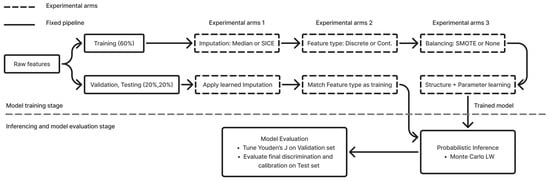
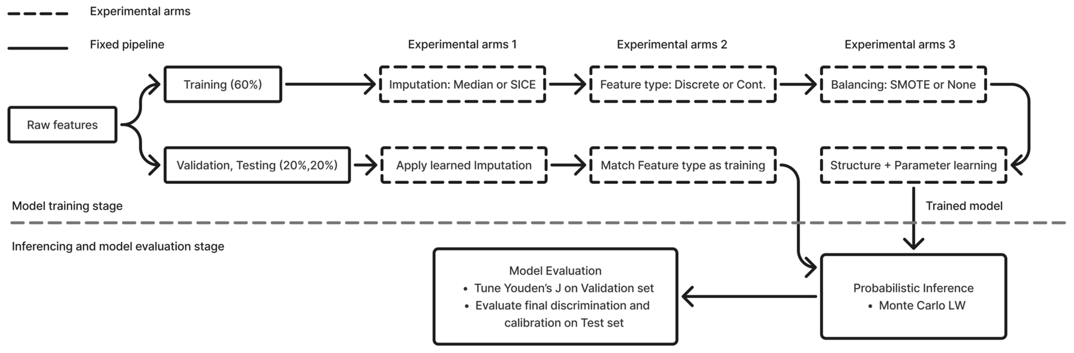
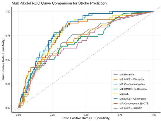
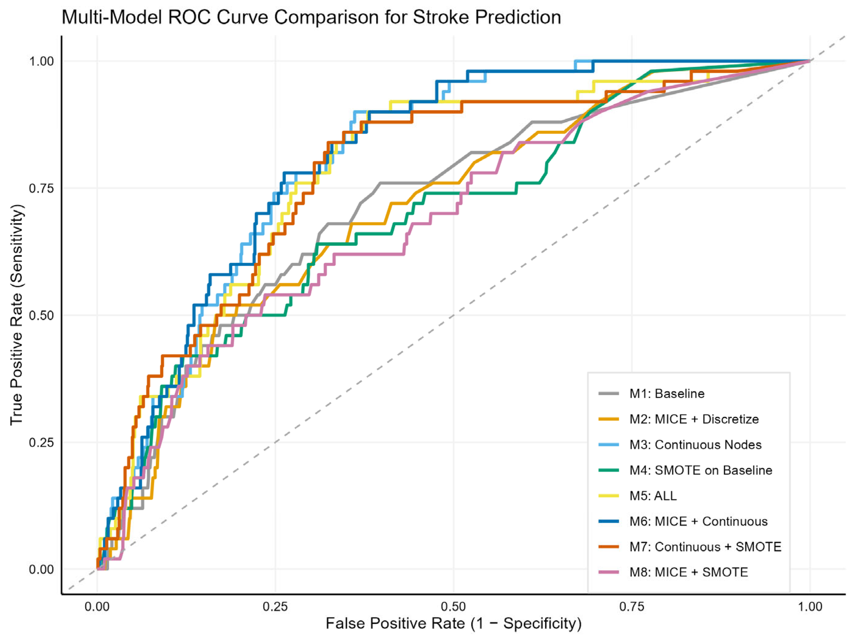
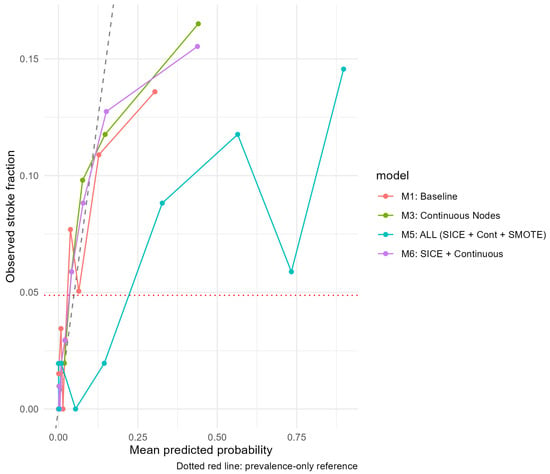
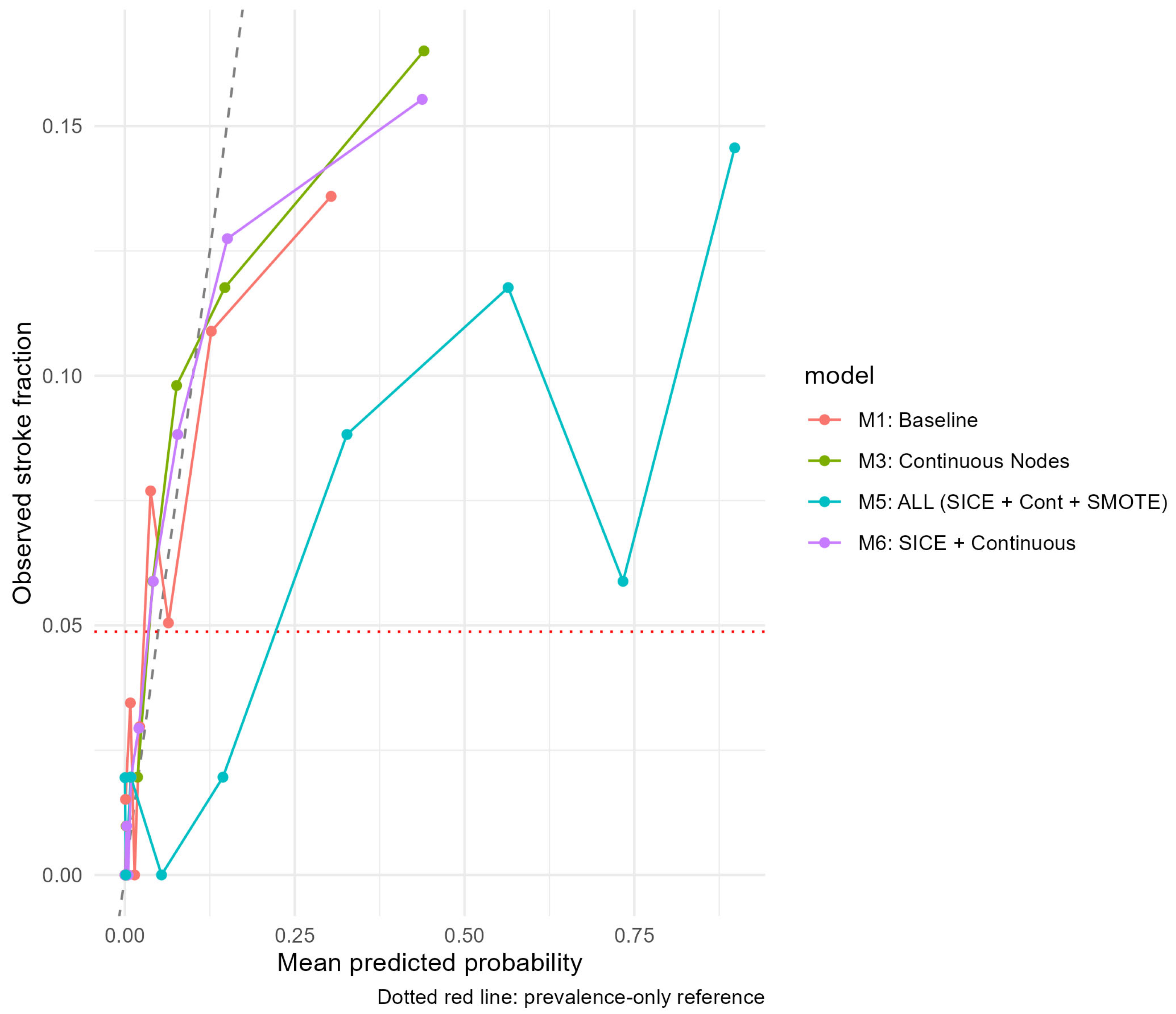
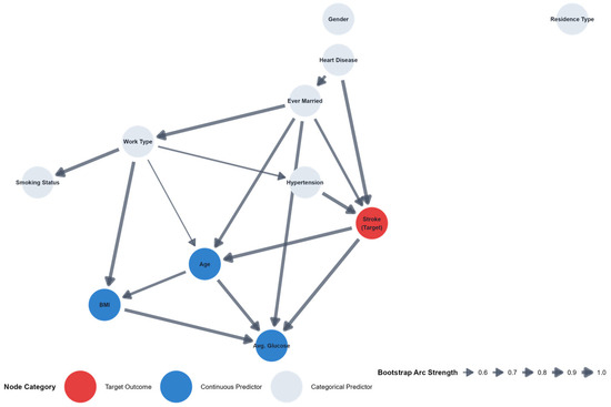
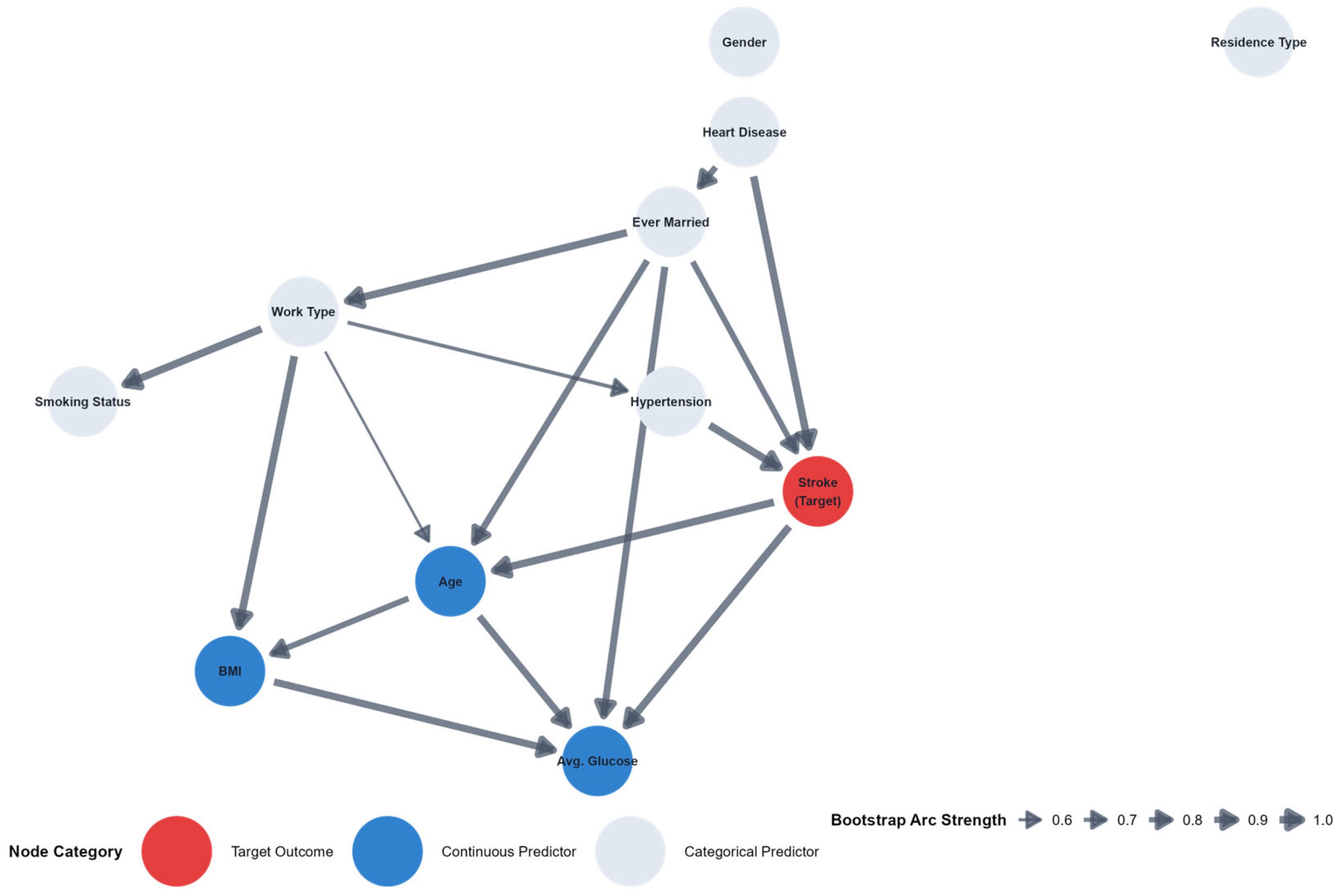

Disclaimer/Publisher’s Note: The statements, opinions and data contained in all publications are solely those of the individual author(s) and contributor(s) and not of MDPI and/or the editor(s). MDPI and/or the editor(s) disclaim responsibility for any injury to people or property resulting from any ideas, methods, instructions or products referred to in the content. |
© 2026 by the authors. Licensee MDPI, Basel, Switzerland. This article is an open access article distributed under the terms and conditions of the Creative Commons Attribution (CC BY) license.