LTFP: Lead-Time-Aware Failure Prediction Based on Service GNNs for AIOps

Abstract

Failures in cloud-native systems can disrupt service availability and system reliability, while their early symptoms are often weak and dispersed across metrics, logs, traces, and interdependent services. Existing methods commonly flatten heterogeneous telemetry or model monitoring variables without preserving service identities. We propose LTFP, a lead-time-aware failure-prediction framework whose graph nodes represent services. LTFP uses modality-specific temporal encoders and gated fusion to form service states, as well as an edge-weight-aware Graph Attention Network to propagate these states over a sparse hybrid graph constructed from known dependencies and training-fitted correlations. Joint graph-level and node-level heads predict whether a failure will occur within a configured future window and rank likely responsible services. We evaluate LTFP on seven subsets from three representative cloud-native systems. Comparisons with representative source-code baselines are reported at the pipeline level, with each method retaining its original learning objective and input configuration. At the 600 s prediction-window setting, LTFP obtains a macro-average window-level precision, recall, and F1 of 92.0%, 90.4%, and 90.5%, respectively. Together with the localization and ablation results, these findings support the effectiveness of service-centered multimodal modeling under the evaluated protocol.

1. Introduction

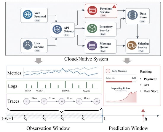
Cloud-native applications are commonly implemented as collections of fine-grained microservices deployed across heterogeneous infrastructure, including containers, hosts, databases, message queues, and service-mesh components [1,2]. At scale, these deployments form large service graphs whose application- and infrastructure-level dependencies increase performance variability and complicate monitoring and fault diagnosis [2,3]. Failures in such systems can disrupt service availability, degrade system performance, and ultimately affect users [4]. Predicting an impending failure is therefore important because it gives operators time to investigate early symptoms and take mitigation measures before the failure fully manifests [5]. As illustrated in Figure 1, the studied task uses multimodal observations and service interactions collected within an observation window to predict whether a failure will occur within a future prediction window and to rank the likely responsible services.

Figure 1. Overview of the studied failure-prediction task. At decision time t, the model uses service-level metric, log, and trace observations collected within the observation window $[t-w+1,t]$ to estimate whether a failure will occur within the future prediction window $(t,t+h]$. It simultaneously outputs the failure probability ${\widehat{p}}_t$ and responsibility scores ${\mathbf{s}}_t$ for ranking the likely responsible services.

To reduce the effort required to continuously monitor complex cloud-native systems, Artificial Intelligence for IT Operations (AIOps) has increasingly been applied to automate failure detection and prediction [4,5]. Cloud-native systems generate three main types of monitoring data. Metrics record numerical changes in resource utilization and service performance, such as CPU utilization, error rate, and response latency. Logs describe runtime events through semi-structured messages, while traces record request paths and interactions among services [6]. Existing failure-prediction approaches mainly learn abnormal patterns from metric time series, and recent work has improved their applicability to dynamically scaling systems by transforming variable-size metric sets into stable model inputs [5]. However, many time-series approaches represent monitoring signals as flat numerical sequences [7,8,9,10]. Such representations can obscure modality-specific temporal patterns and interactions among dependent services. Because early failure symptoms may be weak and distributed across modalities and services [6,11,12], important warning evidence can consequently be missed, reducing prediction accuracy. Cloud-native failure prediction therefore requires a unified representation that combines multimodal temporal evidence with cross-service relationships while retaining service identities for subsequent localization.

Challenges. Achieving these goals requires addressing two key technical gaps:

• Multimodal temporal representation and fusion. Metrics are continuous numerical sequences, logs are sparse event sequences, and traces describe request-level invocation behavior. These modalities have different structures and temporal patterns [6,11,13]. Representing them with a single shared encoder or directly concatenating their raw features can obscure modality-specific information and allow dense metric features to dominate sparse log or trace evidence [6,14]. The challenge is to preserve the temporal characteristics of each modality while learning how much each modality contributes to failure prediction.
• Cross-service relationship modeling. Failure-related changes are often distributed across interacting services [11,12,15]. Known service dependencies describe possible propagation paths, but they may not capture runtime relationships reflected in monitoring data; correlations alone, however, may introduce spurious connections [9,14]. The challenge is to combine structural dependencies with data-driven relationships while preserving service-level representations for responsible-service ranking.

Our Approach. To address these challenges, we propose LTFP, a lead-time-aware failure-prediction framework organized around services rather than individual telemetry variables. Each graph node corresponds to a service, and modality-specific temporal encoders preserve the distinct evolution of its metrics, logs, and traces before gated fusion. LTFP complements known service dependencies with a sparse correlation graph fitted only on training telemetry; the fitted graph is reused at inference instead of being reconstructed for each window. An edge-weight-aware Graph Attention Network propagates evidence across these service nodes. The resulting service-centered representation is shared by a graph-level failure head and a node-level responsibility head, thereby coupling lead-time-specific warning with responsible-service ranking in one multi-task model. This combination distinguishes LTFP from GNN-based anomaly detectors that model feature dimensions and from reactive AIOps methods that localize causes only after an incident is observed.

Contributions. The main contributions of this paper are summarized as follows:

• We formulate proactive failure prediction as service-centered multimodal graph learning: modality-specific temporal encoders preserve the different dynamics of metrics, logs, and traces, while gated fusion retains an explicit representation for every service.
• We construct a sparse, training-fitted hybrid service graph that uses known dependencies as structural edges and correlation edges as data-derived complements. An edge-weight-aware GAT shares the resulting service states between a graph-level warning head and a node-level responsible-service ranker.
• We evaluate the framework on seven RCAEval subsets from three cloud-native systems. Under the 600 s setting, LTFP obtains a macro-average precision, recall, and F1 of 92.0%, 90.4%, and 90.5%, respectively; prediction-window sensitivity, localization, and component analyses characterize its behavior under the stated evaluation protocol.

The remainder of this paper is organized as follows. Section 2 reviews related work. Section 3 defines the task and notation. Section 4 presents LTFP. Section 5 reports the experimental evaluation, and Section 6 concludes the paper.

2. Related Work

Time-series anomaly detection and forecasting. Multivariate time-series anomaly detection is a central line of AIOps research. Classical methods identify abnormal points through reconstruction errors or forecasting residuals, while recent neural models use stochastic recurrent networks, transformers, and graph attention to capture complex temporal dependencies. OmniAnomaly models stochastic latent variables for robust multivariate anomaly detection [7]. TranAD introduces transformer-based adversarial reconstruction for multivariate time series [10], whereas MTAD-GAT combines temporal modeling with feature-level graph attention [8]. Autoformer uses series decomposition and an auto-correlation mechanism for long-horizon forecasting [16]. PatchTST represents time series as patches and applies channel-independent transformer encoders [17]. TimesNet maps temporal variation into a two-dimensional representation for general time-series analysis [18]. Despite their effectiveness, these methods are usually designed for point-level anomaly detection or generic forecasting over flat multivariate sequences. They do not explicitly optimize a lead-time-specific warning window while preserving service-level root-cause localization.

Graph-based and multimodal AIOps. Graph modeling has been widely adopted to represent service dependencies, telemetry correlations, and fault propagation in cloud-native systems. DeepTraLog combines traces and logs with graph-based deep learning for microservice anomaly detection [13]. MicroRCA constructs an attributed service–host graph and correlates service-level performance symptoms with resource utilization [15]. Eadro jointly models intra-service behavior and inter-service dependencies from traces, logs, and metrics [11], while TrinityRCL uses multiple telemetry types to construct a multi-granular graph for fine-grained root-cause localization [12]. Graph-based incident extraction and diagnosis methods use service topology or dependency relations to support large-scale incident analysis [19], while hybrid graph representations have been explored for multimodal microservice anomaly detection [14]. GDN learns relationships among multivariate time-series dimensions and applies graph neural networks for anomaly detection [9]. These studies demonstrate the value of relational inductive bias, but many of them either model metric variables rather than service entities or focus on post-symptom detection and diagnosis. Moreover, known topology may omit statistical relationships caused by shared resources, co-located services, or synchronized workload changes. LTFP therefore constructs a hybrid service graph that combines known dependency edges with correlations fitted exclusively from training telemetry and propagates modality-fused service states over this graph for proactive prediction.

Root cause analysis and alert management. Root cause analysis and alert management are closely related to early fault prediction because they also aim to reduce operational diagnosis effort in complex service systems. Surveys of microservice AIOps highlight the importance of combining metrics, logs, traces, and topology for anomaly detection and root cause analysis [4]. RCAEval provides public fault-injection datasets and baselines for evaluating microservice root-cause localization [20]. Alert storm handling, linked-incident identification, and knowledge-aware alert aggregation reduce noisy alerts after faults have manifested [21,22,23]. Recent multimodal and LLM-assisted RCA approaches further improve post-failure reasoning over heterogeneous observability signals [24]. However, these methods are primarily reactive: they analyze abnormal telemetry or alert streams after an incident is already visible. LTFP moves the decision point earlier by predicting whether a fault will occur within a configured future prediction window and by returning a responsible-service ranking for subsequent diagnosis.

Existing GNN-based AIOps methods either construct relations among monitoring variables for anomaly detection [8,9] or use service graphs for post-failure diagnosis and localization [11,12]. In contrast, LTFP represents services as persistent graph nodes, preserves modality-specific temporal patterns, fits a sparse hybrid graph using only training telemetry, and jointly performs configurable future-window failure prediction and responsible-service ranking. This service-centered and proactive formulation distinguishes LTFP from feature-level anomaly detectors and reactive graph-based diagnosis methods.

3. Preliminaries and Problem Formulation

We first introduce the system, monitoring data, and failure concepts needed to formulate the prediction task.

Definition 1

(Service Graph). A cloud-native application consists of a set of interacting services V. We represent their invocation and operational dependencies as a service graph $G=(V,E)$, where E is the set of directed dependency edges between services.

During operation, each service continuously produces three types of monitoring data [6]:

• Metric. Metrics are numerical measurements of system properties, such as CPU utilization, memory usage, request rate, and response latency. The metric feature vector of service v at timestamp $\tau$ is denoted by ${\mathbf{m}}_{v,\tau }$.
• Log. Logs are semi-structured events that record the runtime state of a service, including warnings, exceptions, and retries. The log feature vector of service v at timestamp $\tau$ is denoted by ${\mathbf{l}}_{v,\tau }$.
• Trace. Traces record the invocation paths of requests as sequences of spans. The trace feature vector of service v at timestamp $\tau$, denoted by ${\mathbf{r}}_{v,\tau }$, summarizes behavior such as call frequency, latency, and error status.

Here, $v\in V$ denotes a service, and $\tau$ denotes a timestamp. We use ${\mathbf{x}}_{v,\tau }=[{\mathbf{m}}_{v,\tau },{\mathbf{l}}_{v,\tau },{\mathbf{r}}_{v,\tau }]$ to denote the combined observation of service v at timestamp $\tau$. The three modalities are complementary because a developing failure may appear in only part of the monitoring data.

Definition 2

(Failure and responsible service). A failure is an event in which the application delivers an incorrect or unavailable service and consequently degrades the user experience. The responsible service is the service in which the fault causing the failure originates. Before a failure becomes visible to users, its developing error state may produce observable symptoms in metrics, logs, or traces.

Problem definition. At decision time t, let w be the number of past timestamps used by the predictor. Its input is

$$X_t=\left\{{\mathbf{x}}_{v,\tau }\mid v\in V,\tau =t-w+1,\dots ,t\right\},$$

(1)

where $X_t$ contains the metric, log, and trace observations of every service from timestamp $t-w+1$ through t. Let h be the length of the configured future prediction window, and let T denote the failure reference time associated with the current case. The prediction label at time t is

$$y_t=\left\{\begin{array}{cc}1,\hfill & 0<T-t\le h,\hfill \\ 0,\hfill & \mathrm{otherwise},\hfill \end{array}\right.$$

(2)

where $y_t=1$ indicates that the failure reference time T lies within h seconds after decision time t. In the evaluated protocol, $T_{\mathrm{inj}}$ is the fault-activation timestamp recorded by the benchmark, whereas T is the first post-activation time at which the entry-service request error rate or P95 response latency satisfies the sustained-violation rule described in Section 5. Thus, $T\ge T_{\mathrm{inj}}$. A candidate observation window ends at $t<T$ and contains only measurements available through t; its future prediction interval is $(t,t+h]$. To avoid labeling pre-activation behavior as an early failure symptom, retained positive windows additionally satisfy $t\ge T_{\mathrm{inj}}$, equivalently $max(T-h,T_{\mathrm{inj}})\le t<T$. Given $X_t$ and the service graph G, the goal is to learn

$$f_{\theta }(X_t,G)=\left({\widehat{p}}_t,{\mathbf{s}}_t\right),$$

(3)

where $f_{\theta }$ is the predictor with learned parameters $\theta$, ${\widehat{p}}_t$ is the predicted probability that $y_t=1$, and ${\mathbf{s}}_t={\left(s_{v,t}\right)}_{v\in V}$ contains one responsibility score $s_{v,t}$ for each service v. Ranking the services by these scores identifies the most likely responsible service. Thus, the task is to estimate failure risk for a configured future interval while identifying the service most likely responsible for the predicted failure.

Example 1.

Figure 1 illustrates this formulation using a cloud-native application in which the Payment Service interacts with the API Gateway and the Data Store through the service graph G. During the observation window $[t-w+1,t]$, the metric, log, and trace sequences of all services constitute $X_t$. At decision time t, the illustrated predictor assigns a failure probability of ${\widehat{p}}_t=0.87$ to the future prediction window $(t,t+h]$ and ranks Payment Service ahead of API Gateway and Data Store according to ${\mathbf{s}}_t$. If the recorded failure reference time T lies within this window, then $y_t=1$; the ranking identifies Payment Service as the most likely responsible service.

4. Methodology

4.1. Overview

As discussed in Section 1, impending failures in cloud-native systems are reflected in two complementary forms of evidence: modality-specific temporal changes within individual services and relational patterns across services. Within each service, metrics, logs, and traces capture different aspects of its evolving state and exhibit distinct temporal patterns. Across services, dependency structures and runtime relationships indicate how failure-related symptoms propagate or co-occur throughout the system. Capturing the first form of evidence requires modality-aware temporal modeling, whereas capturing the second requires service-level graph modeling. Modeling either dimension alone may overlook important warning signals and therefore cannot provide a complete representation for failure prediction and responsible-service ranking.

Motivated by this observation, we propose LTFP, a multimodal temporal failure-prediction framework built around a service-level graph neural network (GNN) for cloud-native systems. Rather than flattening all monitoring features into a single global sequence, LTFP organizes observations around services, learns the temporal behavior of each modality, treats the modality-fused representations as graph-node features, and propagates the resulting service states over a hybrid service graph. This service-centered graph representation is shared by the failure predictor and the responsible-service ranker. At decision time t, LTFP takes the multimodal history $X_t$ and service graph G as input and produces the failure probability ${\widehat{p}}_t$ and service responsibility scores ${\mathbf{s}}_t$ defined in Equation (3).

The framework consists of two core modules:

• Multimodal service-level temporal learning. Raw metrics, logs, and traces are aligned into a temporal history for each service. Modality-specific temporal encoders preserve the distinct temporal patterns of each modality, and a learned gate combines their complementary evidence into a unified service state.
• Hybrid service-graph construction and GNN propagation. Known service dependencies are complemented with correlations fitted from the training data. An edge-weight-aware Graph Attention Network (GAT) then performs message passing among related service nodes. Two jointly trained heads use the resulting graph-level and node-level representations to estimate risk for the configured prediction window and rank the likely responsible services, respectively.

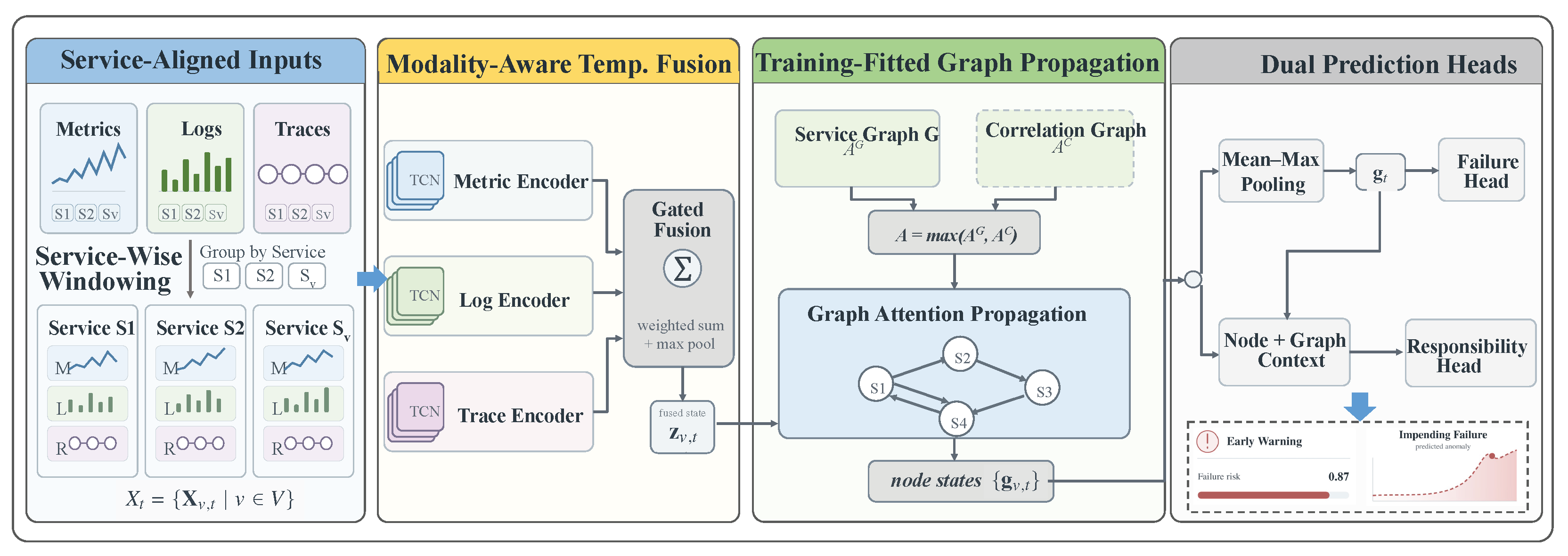
Figure 2 presents the overall framework of LTFP.

Figure 2. Overview of LTFP. Available multimodal observations are converted into service-level temporal node representations and propagated by an edge-weight-aware GNN over a training-fitted hybrid service graph. The resulting graph-level and node-level representations are decoded into a prediction-window-specific failure probability and responsible-service scores, respectively.

4.2. Algorithm

This subsection presents the detailed algorithmic components of LTFP. We first describe service-level observation-window construction and modality-aware temporal fusion (Section 4.2.1), then present the training-fitted hybrid service graph, graph propagation, and joint prediction heads (Section 4.2.2), and finally summarize the multi-task training and inference procedure (Section 4.2.3).

4.2.1. Service-Level Representation Learning

Window construction. Metrics are grouped by service, logs are aggregated into per-service counts, and traces are summarized by service-level duration and error features. As in Section 3, the observation of service v at timestamp $\tau$ and its local history at decision time t are

$${\mathbf{x}}_{v,\tau }=\left[{\mathbf{m}}_{v,\tau };{\mathbf{l}}_{v,\tau };{\mathbf{r}}_{v,\tau }\right],{\mathbf{X}}_{v,t}=\left[{\mathbf{x}}_{v,t-w+1},\dots ,{\mathbf{x}}_{v,t}\right],$$

(4)

where w is the observation-window length and $X_t=\{{\mathbf{X}}_{v,t}\mid v\in V\}$. Feature selection is balanced across services and available modalities so that dense metric features do not suppress sparse log or trace features. If a modality is unavailable, its modality-specific temporal encoder is skipped, and ${\mathbf{x}}_{v,\tau }$ contains only the available feature vectors. For each selected feature, its difference from the preceding timestamp is appended to represent short-term temporal change.

This construction accommodates different monitoring coverage without forcing all datasets into the same raw feature schema. More importantly, it makes the downstream graph operate on services rather than on arbitrary feature columns, which is necessary for responsible-service ranking.

The observation window is generated with a fixed stride over each case timeline. For the configured prediction-window length h, a window ending at t receives the label $y_t$ from Equation (2); it is positive when $T-h\le t<T$, where T is the failure reference time defined in Section 3. Windows ending at or after T are excluded.

Modality-aware temporal fusion. Each available modality is processed by a modality-specific temporal encoder implemented with temporal convolutions and attention pooling over the observation window. For $q\in \{m,l,r\}$, where q indexes the metric, log, or trace modality, the encoder produces

$${\mathbf{z}}_{v,t}^q={\mathrm{Enc}}_q\left({\mathbf{X}}_{v,t}^q\right),$$

(5)

where ${\mathbf{X}}_{v,t}^q$ is the modality-q part of ${\mathbf{X}}_{v,t}$. The modality-specific temporal encoders use the same hidden dimension but do not share temporal parameters. This avoids assuming that metric spikes, log bursts, and trace-latency changes have identical temporal patterns.

The encoded modality states are then combined by a learned gate:

$${\beta }_{v,t}^q={\displaystyle \frac{exp\left({\mathbf{a}}^{\top }{\mathbf{z}}_{v,t}^q\right)}{{\sum }_{q^{\prime }}exp\left({\mathbf{a}}^{\top }{\mathbf{z}}_{v,t}^{q^{\prime }}\right)}},{\mathbf{z}}_{v,t}=\psi \left(\left[\sum _q{\beta }_{v,t}^q{\mathbf{z}}_{v,t}^q;\underset{q}{max}{\mathbf{z}}_{v,t}^q\right]\right).$$

(6)

Here, ${\beta }_{v,t}^q$ is the learned importance of modality q for service v at time t, $\mathbf{a}$ is a learned attention vector, and $\psi$ is a projection network. The weighted term captures the modality mixture, while max pooling retains strong modality-specific evidence. When only one modality is present, Equation (6) operates on the output of a single modality-specific temporal encoder.

4.2.2. Training-Fitted Hybrid Service Graph and GNN-Based Prediction

Training-fitted service graph. The service graph $G=(V,E)$ introduced in Section 3 encodes known invocation and operational dependencies, providing a structural prior for message passing. However, these recorded dependencies may omit runtime associations caused by shared resources, service co-location, or synchronized workload changes. LTFP therefore forms a hybrid graph by complementing the known dependency edges with correlation edges fitted from normalized training telemetry. These correlation edges represent statistical co-variation rather than asserted causal dependencies. The correlation component is fitted only from training windows and is then held fixed for validation and testing; it never uses test labels or test telemetry.

Let $A^G\in {\{0,1\}}^{\left|V\right|\times \left|V\right|}$ be the adjacency matrix constructed from the dependency edges E. The implementation symmetrizes these edges for bidirectional message passing. If explicit dependency information is unavailable, $A^G$ may be empty; self-loops are still inserted so that each service preserves its own representation.

Let ${\mathcal{B}}_{\mathrm{train}}$ denote the training windows after case-level splitting and training-fitted normalization. For each service $v_i$, a scalar activity-magnitude summary is computed for every training window b:

$$u_i^{\left(b\right)}={\displaystyle \frac{1}{w{F}_i}}{\displaystyle \sum _{\tau =1}^w}{\displaystyle \sum _{f=1}^{F_i}}\left|{\tilde{x}}_{i,\tau ,f}^{\left(b\right)}\right|,b\in {\mathcal{B}}_{\mathrm{train}},$$

(7)

where $F_i$ is the number of selected features of service $v_i$ and ${\tilde{x}}_{i,\tau ,f}^{\left(b\right)}$ is its normalized feature f at position $\tau$ in window b. The vector ${\mathbf{u}}_i={\left[u_i^{\left(b\right)}\right]}_{b\in {\mathcal{B}}_{\mathrm{train}}}$ summarizes the normalized activity magnitude of service $v_i$ across training windows. The absolute, normalized activity magnitude is used as a compact service-level statistic because services whose telemetry becomes jointly active across the same training windows may share a runtime relation even when the exported dependency graph omits it. Averaging across timestamps and selected features also prevents services with more raw columns from receiving a mechanically larger graph weight. This statistic intentionally captures window-level co-activity rather than causal propagation. It discards within-window ordering and lag structure, so two services with shifted or short-lived interactions may receive a weak correlation. Correlation edges are obtained from absolute Pearson correlations and sparsified row-wise:

$$A_{ij}^C=\left\{\begin{array}{cc}\left|\rho \right({\mathbf{u}}_i,{\mathbf{u}}_j\left)\right|,\hfill & j\in {TopK}_k\left(i\right),\hfill \\ 0,\hfill & \mathrm{otherwise},\hfill \end{array}\right.A=max(A^G,A^C).$$

(8)

Here, $\rho$ is the Pearson correlation, k is the number of retained neighbors, $A^C$ is the training-fitted correlation adjacency, and A is the final hybrid message-passing adjacency. Constant or missing activity vectors are assigned zero correlation. The fitted A is reused for all training mini-batches and for inference; it is data-driven but does not change with individual validation or test windows.

The row-wise Top-k operation imposes a fixed upper bound on the number of correlation neighbors contributed by each service. It suppresses weak dense correlations and changes sparse message passing from a potential $O\left(\right|V{|}^2)$ neighborhood to $O\left(\right|V\left|k\right)$. The retained experiment uses the value of k recorded in the released configuration, and the same fitted neighbor set is held fixed for validation and testing. In $A=max(A^G,A^C)$, the two sources are not averaged: a known dependency has binary weight 1 and is therefore preserved, whereas a correlation in $[0,1]$ mainly adds an edge when the dependency graph has no corresponding link. The current formulation does not learn a global trade-off between the two edge sources, although the GAT learns content-dependent attention over the retained neighbors.

Because the fitted correlation graph is fixed after training, it does not automatically follow concept drift, service scaling, or topology changes. A production implementation can periodically refit $A^C$ from a recent, operator-confirmed normal interval, validate the candidate graph offline, and deploy it as a versioned artifact with rollback to the previous graph.

Graph propagation and prediction heads. The fused service representations are refined by graph attention layers that use positive entries of A as the edge mask and their magnitudes as an attention prior. For graph layer ℓ, the propagation is written as

$${\mathbf{H}}_t^{(\mathcal{l}+1)}=LayerNorm\left({\mathbf{H}}_t^{\left(\mathcal{l}\right)}+{GAT}_{\mathcal{l}}({\mathbf{H}}_t^{\left(\mathcal{l}\right)},A)\right),{\mathbf{H}}_t^{\left(0\right)}={\left\{{\mathbf{z}}_{v,t}\right\}}_{v\in V}.$$

(9)

Here, ${\mathbf{H}}_t^{\left(\mathcal{l}\right)}$ contains the representations of all services after layer ℓ. The final node representation ${\mathbf{g}}_{v,t}$ is the row of ${\mathbf{H}}_t^{\left(L_g\right)}$ corresponding to service v, where $L_g$ is the number of graph layers, and ${\mathbf{g}}_t$ is the graph-level representation obtained by mean–max pooling over all ${\mathbf{g}}_{v,t}$.

The failure head maps ${\mathbf{g}}_t$ to the probability that $y_t=1$, namely, that the failure reference time T lies within h seconds after decision time t:

$${\widehat{p}}_t=\sigma \left({\mathrm{MLP}}_f\left({\mathbf{g}}_t\right)\right),$$

(10)

where $\sigma$ is the sigmoid function and ${\mathrm{MLP}}_f$ is the failure prediction head.

The responsibility head scores each service using its local representation and the graph-level representation:

$$s_{v,t}={\mathrm{MLP}}_s\left([{\mathbf{g}}_{v,t};{\mathbf{g}}_t;{\mathbf{g}}_{v,t}\odot {\mathbf{g}}_t]\right).$$

(11)

Here, ${\mathrm{MLP}}_s$ is shared by all services and ⊙ denotes element-wise multiplication. The resulting ${\mathbf{s}}_t={\left(s_{v,t}\right)}_{v\in V}$ is exactly the responsibility-score vector defined in Equation (3).

4.2.3. Multi-Task Training and Inference Procedure

Training objective. For a mini-batch $\mathcal{B}$, the failure-prediction loss is

$${\mathcal{L}}_{\mathrm{pred}}={\displaystyle \frac{1}{\left|\mathcal{B}\right|}}\sum _{b\in \mathcal{B}}\mathrm{BCE}({\widehat{p}}_b,y_b),$$

(12)

where ${\widehat{p}}_b$ and $y_b$ are the predicted probability and binary label of window b, respectively. Positive-class weights are estimated from training labels and applied within the binary cross-entropy. Let ${\mathcal{B}}_{+}=\{b\in \mathcal{B}\mid y_b=1\}$ be the positive windows with an available responsible-service label. The responsibility loss is

$${\mathcal{L}}_{\mathrm{resp}}={\displaystyle \frac{1}{|{\mathcal{B}}_{+}|}}\sum _{b\in {\mathcal{B}}_{+}}\mathrm{CE}({\mathbf{s}}_b,v_b^{\ast }),$$

(13)

where ${\mathbf{s}}_b$ contains the responsibility scores for window b and $v_b^{\ast }$ is its true responsible service. The complete objective is

$$\mathcal{L}={\mathcal{L}}_{\mathrm{pred}}+{\lambda }_{\mathrm{resp}}{\mathcal{L}}_{\mathrm{resp}},$$

(14)

where ${\lambda }_{\mathrm{resp}}$ controls the contribution of responsible-service supervision. The second term is omitted when a mini-batch contains no labeled positive window.

Algorithm 1 summarizes the multi-task training and inference procedure. In the algorithm, $\mathbf{X}$, $\mathbf{Y}$, and $\mathbf{R}$ denote the constructed windows, their binary failure labels, and their responsible-service labels, respectively.

Algorithm 1: LTFP

Input: cases $\mathcal{C}$, service graph G, observation-window length w, prediction-window length h, graph sparsity k, epochs $N_e$ Output: learned parameters $\theta$, failure probability ${\widehat{p}}_t$, responsibility scores ${\mathbf{s}}_t$ 1: $(\mathbf{X},\mathbf{Y},\mathbf{R})\leftarrow \mathrm{Windowize}(\mathcal{C},w,h)$ 2: Split cases into ${\mathcal{C}}_{\mathrm{train}}$ and ${\mathcal{C}}_{\mathrm{test}}$ without case overlap 3: Fit normalization statistics on training windows and transform all windows 4: Construct $A^G$ from G and fit $A^C$ on training windows 5: $A\leftarrow max(A^G,A^C)$ 6: Initialize model parameters $\theta$ 7: for $e=1,\dots ,N_e$ do 8:     for mini-batch $\mathcal{B}$ of training windows do 9:         for available modality $q\in \{m,l,r\}$ do 10:            ${\mathbf{Z}}^q\leftarrow {\mathrm{Enc}}_q({\mathbf{X}}_{\mathcal{B}}^q;\theta )$ 11:         $\mathbf{Z}\leftarrow \mathrm{Fuse}\left({\left\{{\mathbf{Z}}^q\right\}}_q\right)$ 12:         $\mathbf{H}\leftarrow \mathrm{EdgeWeightAwareGAT}(\mathbf{Z},A;\theta )$ 13:         $(\widehat{\mathbf{p}},\mathbf{S})\leftarrow \mathrm{Predict}(\mathbf{H};\theta )$ 14:         $\mathcal{L}\leftarrow {\mathcal{L}}_{\mathrm{pred}}+{\lambda }_{\mathrm{resp}}{\mathcal{L}}_{\mathrm{resp}}$ 15:         $\theta \leftarrow \mathrm{Adam}(\theta ,{\nabla }_{\theta }\mathcal{L})$ 16: Apply the same normalization and fitted graph A to test windows 17: return ${\widehat{p}}_t$ and ${\mathbf{s}}_t$ for each test window

The two loss terms correspond directly to the two outputs in Equation (3). Failure supervision trains the prediction-window-specific warning decision, while responsible-service supervision keeps the node representations useful for localization.

4.3. Complexity Analysis

Let B be the number of windows, $B_{\mathrm{train}}$ the number of training windows, $\left|V\right|$ the number of services, F the maximum selected feature width per service, d the hidden dimension, $L_t$ the number of temporal layers, $L_g$ the number of graph attention layers, and k the correlation-graph sparsity. Service-level window construction costs $O\left(B\right|V\left|wF\right)$. Modality-specific temporal encoding costs $O\left(B\right|V\left|L_{t}w{d}^2\right)$, with smaller constants when some modalities are absent. Fitting the correlation graph costs $O\left(B_{\mathrm{train}}\right|V\left|wF\right)$ for activity-magnitude summaries and $O\left(B_{\mathrm{train}}\right|V{|}^2)$ for service-pair correlations.

Dense graph propagation costs $O\left(B{L}_g\right|V{|}^{2}d)$ per epoch, while sparse propagation over the Top-k graph costs $O\left(B{L}_g\right|V\left|kd\right)$. The failure head costs $O\left(Bd\right)$ and the responsibility head costs $O\left(B\right|V\left|d\right)$. The main memory usage is $O\left(B\right|V\left|wF\right)$ for window tensors, $O\left(\right|V{|}^2)$ for a dense adjacency matrix or $O\left(\right|V\left|k\right)$ for a sparse one, and $O\left(B\right|V\left|d\right)$ for service states.

During inference, normalization statistics and the training-fitted hybrid graph are reused unchanged. Therefore, the online cost is dominated by temporal encoding, graph propagation, and the two prediction heads; no test-label-dependent or per-window graph construction is performed.

5. Experimental Evaluation

This section evaluates LTFP on RCAEval benchmark subsets. The evaluation answers five questions: (1) how LTFP compares numerically with recent source-code pipelines at two selected prediction-window lengths, (2) how performance changes as the configured prediction-window length h varies, (3) whether LTFP can identify responsible services, (4) how efficiently LTFP trains and performs inference, and (5) how the main model components affect prediction at the default $h=600$ s.

5.1. Experimental Setup

Datasets. RCAEval organizes benchmark cases by system and subset family. We evaluate seven processed subsets from three representative cloud-native systems: Online Boutique (OB), Sock Shop (SS), and TrainTicket (TT). In each subset identifier, RE1, RE2, and RE3 denote RCAEval subset families, while OB, SS, and TT denote the benchmark system. Thus, RE1-OB is the RE1 subset of Online Boutique, RE2-SS is the RE2 subset of Sock Shop, and RE3-TT is the RE3 subset of TrainTicket. For constructing the labels in Equation (2), each case supplies a recorded fault-activation time $T_{\mathrm{inj}}$ and the responsible service from its benchmark metadata. Table 1 summarizes the case/window statistics and available modalities.

Table 1. Processed RCAEval subsets, selected feature counts, and telemetry coverage.

System	Subset	Cases	Windows	Selected Features	Available Modalities
Online Boutique	RE1-OB	125	21,625	75	metrics
	RE3-OB	30	3510	117	metrics + logs + traces
Sock Shop	RE1-SS	125	7125	180	metrics
	RE2-SS	90	10,530	40	metrics + logs
	RE3-SS	30	3510	116	metrics + logs
TrainTicket	RE1-TT	125	9125	180	metrics
	RE3-TT	30	4410	180	metrics + logs + traces

RCAEval stores metrics as time-series measurements and, where available, logs and traces as separate telemetry files. The selected feature names are not assumed to be identical across systems. We group columns by modality and service and select them in round-robin order up to the feature budget. The selected-feature count is the number of raw telemetry columns left after this procedure; if fewer columns are available than the budget, all are kept. Table 1 reports these counts, while the exact column names are provided in the repository feature manifests.

Baseline preparation. For follow-up source-code comparisons, we prepare four baselines whose repositories can be executed under the local experimental environment:

• MTAD-GAT [8]: A graph-attention model for multivariate time-series anomaly detection.
• GDN [9]: A graph deviation network that learns relationships among multivariate time-series dimensions.
• TranAD [10]: A transformer-based multivariate anomaly-detection model.
• TimesNet/Time-Series-Library [18]: A general time-series analysis framework instantiated with TimesNet for anomaly detection.

These baselines were selected to cover four distinct and widely used time-series modeling choices: MTAD-GAT represents feature relationships with graph attention; GDN learns a graph among time-series dimensions; TranAD uses transformer-based adversarial reconstruction; and TimesNet is a general temporal backbone based on two-dimensional variation. Together, they provide graph-based, transformer-based, and general temporal anomaly-detection reference pipelines.

For each reported prediction-window length h, all pipelines are evaluated using the same retained windows and exported binary labels $y_t$.

Implementation details. The source code, configuration files, data-processing scripts, dataset-specific feature manifests, and result summaries are available in the LTFP repository (https://github.com/mlk12333/LTFP (accessed on 21 August 2026)). LTFP is implemented in PyTorch 2.12.1 and trained on the CPU. The retained experiments use the settings summarized in Table 2. Hyperparameter selection was deliberately conservative. For LTFP, the reported settings were determined from preliminary training-only runs by considering optimization stability and CPU cost, and they were fixed before the reported test evaluation. For the comparison methods, we followed the default or recommended settings of their public implementations wherever applicable, with only data-dependent adjustments required by the exported input format. All settings were fixed before test evaluation, and the values of h in the sensitivity table define different prediction tasks rather than tuning candidates.

Table 2. Configuration of the retained LTFP experiments.

Group	Parameter	Setting
Windowing	observation length w/stride	24 timestamps/6 timestamps
Task	default/sensitivity h	600 s/$\{60,180,300,900\}$ s
Representation	hidden dimension/TCN layers	32/3
Graph model	GAT layers/correlation sparsity	2/Top-$k=2$
Regularization	dropout	0.12
Optimization	batch size/epochs	32/20 (8 for RE2-SS)
Inputs	LTFP/baseline feature caps	up to 180 raw/up to 80 exported
Partition	model fitting/final testing	70%/30% (case-level)
Reproducibility	random seed/full feature lists	7/repository manifests
Decision	anomaly or class thresholds	training-fitted or source-pipeline rule

The retained protocol uses a 70/30 case-level split with seed 7: 70% of the cases are used for model fitting, and 30% are reserved for final testing, with all windows from one case kept in the same partition.

We adopt a controlled post-activation, pre-user-visible-failure setting. The benchmark supplies $T_{\mathrm{inj}}$. The failure reference time T is determined after activation from the entry-service request error rate or P95 response latency. “Sustained” means that at least three of four consecutive 15 s samples exceed the threshold. Each threshold is fitted on normal training data as $max(q_{0.995},\mathrm{median}+6\times 1.4826\mathrm{MAD})$; floors of 0.05 and $1.5\times \mathrm{median}$ are used for error rate and latency, respectively. No test telemetry or test label is used to fit these thresholds. The positive interval is $max(T-h,T_{\mathrm{inj}})\le t<T$; candidate windows in $[T-h,T_{\mathrm{inj}})$ and windows ending at or after T are excluded.

For external baselines, we use at most 80 exported features, evaluate the same retained windows, and train the unsupervised pipelines on strict normal segments preceding the positive prediction window when available; otherwise, label-zero windows form the normal export. LTFP instead uses failure and responsible-service supervision and at most 180 raw features. Therefore, the following tables are contextual cross-pipeline comparisons, not a controlled comparison of architecture or supervision.

We do not modify the baseline model architectures; the retained windows are only converted to the input formats required by their public implementations, as listed in Table 3.

Table 3. Reproducibility information for the external comparison pipelines. Each pipeline uses the latest public source-code version available when the experiments were conducted.

Pipeline	Key Settings	Input Conversion
MTAD-GAT	lookback 20; batch 64; 1 epoch	SMD-format export
GDN	window/stride 10/5; dim 16; Top-$k=5$; batch 128; 1 epoch	GDN-format export
TranAD	window 10; batch 128; learning rate 0.001; 5 epochs	MSDS-format export
TimesNet	sequence 100; model/FF dim 32; 1 layer; batch 128; 1 epoch	SMD-format export

5.2. Failure Prediction Performance Comparison

We report contextual source-code pipeline results at 300 s and 600 s. Table 4 and Table 5 give window-level precision, recall, and F1 on the same retained windows and prediction-window-specific labels. Each external column preserves the thresholding and reporting procedure of its source anomaly-detection pipeline. Precision and recall are reported alongside F1 because different operating points may favor false-alarm reduction or event coverage. Bold values indicate only numerical row maxima under these heterogeneous pipelines; they do not establish an architecture-level ranking.

Table 4. Window-level results of the completed source-code pipelines using a 300 s prediction window.

Dataset	MTAD-GAT			GDN			TranAD			TimesNet			LTFP
	P	R	F1	P	R	F1	P	R	F1	P	R	F1	P	R	F1
RE1-OB	0.862	0.388	0.537	0.138	0.720	0.231	0.618	0.312	0.415	0.287	0.368	0.323	0.821	0.609	0.699
RE1-SS	0.866	0.395	0.543	0.364	0.653	0.467	0.956	0.312	0.470	0.703	0.512	0.593	0.887	0.990	0.936
RE1-TT	0.721	0.456	0.559	0.319	0.724	0.443	0.893	0.416	0.568	0.647	0.560	0.600	0.699	0.960	0.809
RE2-SS	0.865	0.389	0.538	0.149	0.534	0.233	0.732	0.244	0.366	0.401	0.389	0.395	0.448	0.897	0.597
RE3-OB	0.878	0.384	0.534	0.125	0.449	0.196	0.897	0.667	0.765	0.496	0.567	0.529	0.519	0.800	0.630
RE3-SS	0.869	0.401	0.545	0.125	0.450	0.196	0.696	0.633	0.663	0.472	0.333	0.391	0.670	0.938	0.781
RE3-TT	0.861	0.397	0.542	0.130	0.581	0.212	0.891	0.967	0.927	0.596	0.900	0.717	0.831	0.909	0.868
Average	0.846	0.400	0.541	0.193	0.587	0.283	0.812	0.507	0.596	0.515	0.518	0.507	0.697	0.872	0.760

Note: Bold numbers denote the numerical maximum for each metric within each dataset row or the average row.

Table 5. Window-level results of the completed source-code pipelines using a 600 s prediction window.

Dataset	MTAD-GAT			GDN			TranAD			TimesNet			LTFP
	P	R	F1	P	R	F1	P	R	F1	P	R	F1	P	R	F1
RE1-OB	0.261	0.768	0.390	0.167	0.575	0.258	0.182	0.436	0.257	0.453	0.505	0.478	0.845	0.511	0.637
RE1-SS	0.985	0.808	0.888	0.430	0.643	0.515	0.774	0.144	0.243	0.888	0.864	0.876	1.000	0.983	0.992
RE1-TT	0.891	0.918	0.904	0.507	0.759	0.608	0.846	0.493	0.623	0.918	0.890	0.904	1.000	0.987	0.994
RE2-SS	0.430	1.000	0.601	0.300	0.538	0.386	0.261	0.356	0.301	0.584	0.344	0.433	0.873	0.968	0.918
RE3-OB	0.471	0.967	0.633	0.289	0.519	0.371	0.425	0.767	0.547	0.677	0.500	0.575	0.855	1.000	0.922
RE3-SS	0.530	0.900	0.667	0.314	0.563	0.403	0.579	0.100	0.171	0.816	0.667	0.734	0.922	0.927	0.924
RE3-TT	0.482	1.000	0.651	0.298	0.668	0.412	0.609	1.000	0.757	0.762	0.900	0.825	0.943	0.952	0.947
Average	0.579	0.909	0.676	0.329	0.609	0.422	0.525	0.471	0.414	0.728	0.667	0.689	0.920	0.904	0.905

Note: Bold numbers denote the numerical maximum for each metric within each dataset row or the average row.

At 300 s, LTFP obtains average precision, recall, and F1 of 0.697, 0.872, and 0.760. The operating points differ materially: MTAD-GAT has the highest average precision (0.846) but a recall of 0.400, whereas LTFP accepts lower precision for substantially higher recall. Results are also not uniform across datasets, as TranAD has a higher F1 on RE3-OB and RE3-TT. At 600 s, LTFP obtains 0.920 precision, 0.904 recall, and 0.905 F1, while TimesNet is the strongest external pipeline by average F1 (0.689). These values characterize the complete pipelines under the retained protocol; supervision and feature budget differences preclude attributing the numerical gap solely to the LTFP architecture.

5.3. Effect of Prediction-Window Length

Table 6 reports window-level precision, recall, and F1 when the prediction-window length h is set to five alternative values. Each column evaluates the probability associated with the interval defined by its configured value of h against the corresponding binary labels.

Table 6. LTFP window-level precision, recall, and F1 for alternative prediction-window lengths h.

Dataset	60s			180s			300s			600s			900s
	P	R	F1	P	R	F1	P	R	F1	P	R	F1	P	R	F1
RE1-OB	0.172	0.418	0.244	0.492	0.610	0.545	0.821	0.609	0.699	0.845	0.511	0.637	0.550	0.930	0.691
RE1-SS	0.349	0.440	0.389	0.612	0.910	0.732	0.887	0.990	0.936	1.000	0.983	0.992	0.988	0.980	0.984
RE1-TT	0.134	0.262	0.177	0.457	0.832	0.590	0.699	0.960	0.809	1.000	0.987	0.994	0.994	0.986	0.990
RE2-SS	0.092	0.863	0.166	0.269	0.914	0.416	0.448	0.897	0.597	0.873	0.968	0.918	0.997	1.000	0.998
RE3-OB	0.184	0.540	0.274	0.329	0.747	0.457	0.519	0.800	0.630	0.855	1.000	0.922	0.993	0.995	0.994
RE3-SS	0.132	0.278	0.179	0.475	0.563	0.515	0.670	0.938	0.781	0.922	0.927	0.924	0.991	0.999	0.995
RE3-TT	0.388	0.689	0.496	0.646	0.811	0.719	0.831	0.909	0.868	0.943	0.952	0.947	0.995	1.000	0.997
Average	0.207	0.499	0.275	0.469	0.770	0.568	0.697	0.872	0.760	0.920	0.904	0.905	0.930	0.984	0.950

Classification performance depends on the configured prediction-window length. Average F1 increases from 0.275 at 60 s to 0.905 at 600 s and 0.950 at 900 s as the positive interval widens and contains more positive windows. The corresponding 600 s precision and recall are 0.920 and 0.904. This comparison reflects the difficulty and class balance induced by different label-window widths, rather than measured operational warning lead time. RE1-OB remains the main outlier at 600 s, with high precision but a recall of 0.511.

5.4. Responsible-Service Localization

Table 7 evaluates responsibility scores ${\mathbf{s}}_t$ on positive windows at $h=900$ s because only those windows have a benchmark responsible-service label. Hit@1 checks the first-ranked service, while Hit@3 and Hit@5 check membership within the first three or five positions. We additionally report the number of candidate services, two label-only sanity baselines, and a reciprocal-rank summary. The training-frequency prior ranks candidates by their responsible-label counts in positive training windows; the random baseline is the analytic expectation under a uniformly random permutation of each dataset’s candidate set.

Table 7. Conditional responsible-service localization on positive windows at $h=900$ s. Baseline rows are macro averages. LTFP MRR entries are conservative lower bounds; baseline MRR entries are exact or analytic expectations.

Dataset/Method	Candidates	Hit@1	Hit@3	Hit@5	MRR
RE1-OB	6	0.629	0.851	0.979	≥0.732
RE1-SS	9	0.483	0.808	0.957	≥0.626
RE1-TT	6	0.255	0.622	0.984	≥0.453
RE2-SS	9	0.234	0.601	0.789	≥0.417
RE3-OB	5	0.611	0.974	1.000	≥0.737
RE3-SS	7	0.651	0.999	1.000	≥0.768
RE3-TT	3	0.460	1.000	1.000	≥0.640
LTFP average	–	0.475	0.836	0.958	≥0.625
Training-frequency prior	–	0.297	0.757	1.000	0.553
Random ranking	–	0.176	0.528	0.785	0.412

The retained evaluation artifacts record Hit@1, Hit@3, and Hit@5 but not every per-window rank. We therefore report a conservative lower bound on MRR rather than impute unrecorded ranks. With $H_k$ denoting Hit@k and N the number of candidates, the bound is

$${\mathrm{MRR}}_{\mathrm{LB}}=H_1+{\displaystyle \frac{H_3-H_1}{min(3,N)}}+{\displaystyle \frac{H_5-H_3}{min(5,N)}}+{\displaystyle \frac{1-H_5}{N}}.$$

(15)

It assigns newly observed hits in each interval to the worst rank in that interval, so the exact MRR cannot be lower than the reported value. The sanity baselines’ MRR values are exact or analytic expectations.

At deployment, a service list is emitted only when the failure probability exceeds its training-fitted threshold. Thus, a false failure alarm on a negative window also produces a false localized alert, even though no responsible target exists for scoring its internal order. At $h=300$ s, where every test subset contains negative windows, 4000 of 11,806 negative windows are false positives: the pooled FPR is 0.339, and the macro-average dataset FPR is 0.524 (range 0.054–0.900). At $h=900$ s, the retained negative-window support becomes substantially smaller and highly uneven across subsets, making this setting unsuitable for a stable cross-dataset FPR analysis.

The average Hit@1 of 0.475 indicates that exact single-service localization remains challenging, particularly on RE1-TT and RE2-SS. On macro average, LTFP exceeds the training-frequency prior and random ranking on Hit@1, Hit@3, and the conservative MRR comparison, showing that it learns more than label prevalence or chance. However, Hit@3 must be interpreted relative to candidate-set size, which ranges from three to nine; for RE3-TT, Hit@3 is necessarily 1.000 because only three candidates exist. The frequency prior’s perfect average Hit@5 further shows that large-k membership can saturate without precise ordering. Together with the negative-window false-positive results, these findings support using the ranking only as an auxiliary shortlist, not as an automatic root-cause decision. The two added baselines provide task-compatible reference points rather than direct comparisons with post-failure RCA methods.

5.5. Computational Efficiency

We profiled LTFP on the sampled 30-case RE3-OB protocol using an Arm64 CPU with four PyTorch CPU threads and a batch size of 32. Table 8 reports the parameter count, training time for five epochs, and inference efficiency over 1053 test windows. Data loading and feature construction are excluded.

Table 8. Measured computational efficiency on the sampled RE3-OB protocol.

Trainable Parameters	Training Time (s)	Inference Time (s)	Latency (ms/Window)	Throughput (Windows/s)
12,730	88.1	3.70	3.512	284.7

5.6. Ablation Study

We further analyze the contribution of each LTFP component over all seven RCAEval subsets rather than on a single dataset. To keep this component analysis tractable, all rows in Panel A of Table 9 use the same sampled protocol: a fixed 30-case subset per RCAEval split, 5 epochs, 80 raw features, and a hidden dimension of 16. The full LTFP row is the control model, and each following row removes one component. AUPRC denotes the area under the precision–recall curve and reflects threshold-independent ranking quality under imbalanced window-level labels.

Table 9. Resource-aware component and individual-modality ablation results using the default prediction window $h=600$ s.

Variant/Input	P	R	F1	AUPRC
Panel A: Component ablation averaged over seven RCAEval subsets
Full LTFP	0.829	0.956	0.879	0.900
w/o graph propagation	0.662	0.831	0.737	0.754
w/o responsible-service supervision	0.742	0.883	0.806	0.822
w/o temporal-difference features	0.728	0.874	0.795	0.809
Panel B: Fixed-schema modality ablation on RE3-OB
Metrics + logs + traces	0.855	0.981	0.913	0.867
Metrics only	0.784	0.921	0.847	0.856
Logs only	0.792	0.905	0.845	0.851
Traces only	0.771	0.893	0.828	0.837

Panel B isolates the three data modalities without changing their feature budgets. We first select the same 80-feature RE3-OB schema as the full model and then retain only its metric, log, or trace portion before retraining. RE3-OB is used because this fixed schema contains all three modalities. All variants use the same 30 cases, case split, 5 epochs, and a hidden dimension of 16.

Panel A shows that removing graph propagation causes the largest decrease in F1 and AUPRC. Removing responsible-service supervision or temporal-difference features also reduces both measures, supporting the contribution of relational modeling, localization supervision, and temporal-change information under the sampled protocol.

All three single-modality variants achieve useful performance. The complete multimodal input obtains the highest F1 (0.913), compared with 0.847, 0.845, and 0.828 for metrics, logs, and traces, respectively. This result shows that the three modalities provide complementary information.

The graph-construction and training-trace analyses are summarized in Table 10.

Table 10. Graph-construction analysis at 600 s. Panel A is averaged over seven subsets; Panel B compares retained correlation pairs with training-trace call pairs.

Panel A: Graph Variants
Graph		F1	AUPRC	Top-1	Top-3
Hybrid-max (current)		0.865	0.887	0.649	0.961
Dependency-only		0.828	0.852	0.592	0.932
Correlation-only		0.838	0.860	0.606	0.940
Hybrid-learned		0.849	0.873	0.625	0.949
Hybrid-lagged		0.842	0.866	0.615	0.945
Panel B: Training-Trace Runtime-Edge Proxy
Subset	Corr.	Supported	Precision	Random	Enrichment
RE3-OB	43	8	0.186	0.025	7.55×
RE3-TT	114	15	0.132	0.023	5.73×
Aggregate	157	23	0.146	0.023	6.26×

Note: Bold numbers denote the numerical maximum for each metric in Panel A.

All variants in Panel A use the same sampled protocol. Max fusion achieves the highest F1, AUPRC, Top-1, and Top-3 among the evaluated graph variants, supporting its use to preserve known dependencies while incorporating training-derived correlations. Panel B uses only training traces: 23 of 157 retained correlation pairs match observed calls versus 2.3% for equal-count random pairs. This 6.26-fold enrichment supports a meaningful call-related subset, but it is a runtime-relation proxy rather than causal propagation ground truth.

5.7. Discussion

Interpretation of comparisons. The source-code baselines retain their original learning objectives and input configurations, while all pipelines are evaluated on the same retained windows and binary labels. The reported results therefore characterize end-to-end pipeline performance under the evaluated protocol. Precision, recall, and F1 are considered jointly, while controlled effects of LTFP components are examined separately through the ablation studies.

Practical deployment and maintenance. In deployment, the normalization statistics, service graph, and model parameters are fitted offline and stored as a versioned artifact. Online collectors construct service-aligned multimodal windows, and each completed window is scored to produce a failure probability, prediction window, and ranked service list. The correlation graph can be periodically refreshed using recent confirmed-normal telemetry and deployed after offline validation, with the previous version retained for rollback.

Limitations. LTFP relies on the monitoring patterns and service relations represented in the training data. Rapid workload or topology changes may require a graph refresh, while sustained missing or noisy telemetry may reduce the information available for individual services. These effects can be mitigated through telemetry-quality monitoring, schema checks, and periodic artifact updates.

6. Conclusions

LTFP organizes heterogeneous telemetry around service nodes: separate temporal encoders and gated fusion preserve modality-specific evidence, while a sparse graph combining known dependencies with training-fitted correlations supports cross-service propagation. Shared graph- and node-level heads connect a configurable future-window warning with responsible-service ranking.

Across seven RCAEval subsets, the 600 s setting produces a macro-average precision, recall, and F1 of 92.0%, 90.4%, and 90.5%. At 900 s, conditional positive-window responsible-service Hit@1 and Hit@3 are 47.5% and 83.6%, and the conservative MRR lower bound is 0.625. These values exceed random ranking and a training-frequency prior on macro average, but the modest Hit@1 value, candidate-set dependence, and negative-window false alarms limit the result to an auxiliary shortlist. The baseline results are interpreted at the pipeline level because the evaluated methods retain their original learning objectives and input configurations. Controlled component and modality analyses are reported separately through the ablation studies, while the localization sanity baselines do not establish superiority over prior RCA systems.

The framework provides an early-warning probability and an operator shortlist. Two practical considerations remain: the fixed correlation graph may lag behind rapid workload or topology changes, and persistent missing or noisy telemetry may weaken service representations. Future work will therefore focus on versioned graph maintenance, causal propagation-path validation, and more robust handling of incomplete telemetry.

References

- Mazzara, M.; Meyer, B. (Eds.) Present and Ulterior Software Engineering; Springer: Cham, Switzerland, 2017. [Google Scholar]
- Gan, Y.; Zhang, Y.; Cheng, D.; Shetty, A.; Rathi, P.; Katarki, N.; Bruno, A.; Hu, J.; Ritchken, B.; Jackson, B.; et al. An open-source benchmark suite for microservices and their hardware-software implications for cloud & edge systems. In Proceedings of the Twenty-Fourth International Conference on Architectural Support for Programming Languages and Operating Systems, Providence, RI, USA, 13–17 April 2019; pp. 3–18. [Google Scholar]
- Zhou, X.; Peng, X.; Xie, T.; Sun, J.; Ji, C.; Li, W.; Ding, D. Fault analysis and debugging of microservice systems: Industrial survey, benchmark system, and empirical study. IEEE Trans. Softw. Eng. 2018, 47, 243–260. [Google Scholar] [CrossRef] [Scilit]
- Soldani, J.; Brogi, A. Anomaly detection and failure root cause analysis in (micro) service-based cloud applications: A survey. ACM Comput. Surv. (CSUR) 2022, 55, 1–39. [Google Scholar] [CrossRef] [Scilit]
- Denaro, G.; El Moussa, N.; Heydarov, R.; Lomio, F.; Pezzè, M.; Qiu, K. Predicting failures of autoscaling distributed applications. Proc. ACM Softw. Eng. 2024, 1, 1960–1981. [Google Scholar] [CrossRef] [Scilit]
- Zhao, C.; Ma, M.; Zhong, Z.; Zhang, S.; Tan, Z.; Xiong, X.; Yu, L.; Feng, J.; Sun, Y.; Zhang, Y.; et al. Robust multimodal failure detection for microservice systems. In Proceedings of the 29th ACM SIGKDD Conference on Knowledge Discovery and Data Mining, Long Beach, CA, USA, 6–10 August 2023; pp. 5639–5649. [Google Scholar]
- Su, Y.; Zhao, Y.; Niu, C.; Liu, R.; Sun, W.; Pei, D. Robust anomaly detection for multivariate time series through stochastic recurrent neural network. In Proceedings of the 25th ACM SIGKDD International Conference on Knowledge Discovery & Data Mining, Anchorage, AK, USA, 4–8 August 2019; pp. 2828–2837. [Google Scholar]
- Zhao, H.; Wang, Y.; Duan, J.; Huang, C.; Cao, D.; Tong, Y.; Xu, B.; Bai, J.; Tong, J.; Zhang, Q. Multivariate time-series anomaly detection via graph attention network. In Proceedings of the 2020 IEEE International Conference on Data Mining (ICDM), Sorrento, Italy, 17–20 November 2020; pp. 841–850. [Google Scholar]
- Deng, A.; Hooi, B. Graph neural network-based anomaly detection in multivariate time series. In Proceedings of the AAAI Conference on Artificial Intelligence, Virtual, 2–9 February 2021; pp. 4027–4035. [Google Scholar]
- Tuli, S.; Casale, G.; Jennings, N.R. Tranad: Deep transformer networks for anomaly detection in multivariate time series data. arXiv 2022, arXiv:2201.07284. [Google Scholar]
- Lee, C.; Yang, T.; Chen, Z.; Su, Y.; Lyu, M.R. Eadro: An end-to-end troubleshooting framework for microservices on multi-source data. In Proceedings of the 2023 IEEE/ACM 45th International Conference on Software Engineering (ICSE), Melbourne, Australia, 14–20 May 2023; pp. 1750–1762. [Google Scholar]
- Gu, S.; Rong, G.; Ren, T.; Zhang, H.; Shen, H.; Yu, Y.; Li, X.; Ouyang, J.; Chen, C. Trinityrcl: Multi-granular and code-level root cause localization using multiple types of telemetry data in microservice systems. IEEE Trans. Softw. Eng. 2023, 49, 3071–3088. [Google Scholar] [CrossRef] [Scilit]
- Zhang, C.; Peng, X.; Sha, C.; Zhang, K.; Fu, Z.; Wu, X.; Lin, Q.; Zhang, D. Deeptralog: Trace-log combined microservice anomaly detection through graph-based deep learning. In Proceedings of the 44th International Conference on Software Engineering, Pittsburgh, PA, USA, 21–29 May 2022; pp. 623–634. [Google Scholar]
- Wang, P.; Zhang, X.; Cao, Z. Anomaly detection for microservice system via augmented multimodal data and hybrid graph representations. Inf. Fusion 2025, 118, 103017. [Google Scholar] [CrossRef] [Scilit]
- Wu, L.; Tordsson, J.; Elmroth, E.; Kao, O. Microrca: Root cause localization of performance issues in microservices. In Proceedings of the IEEE/IFIP Network Operations and Management Symposium (NOMS), Virtual, 20–24 April 2020. [Google Scholar]
- Wu, H.; Xu, J.; Wang, J.; Long, M. Autoformer: Decomposition transformers with auto-correlation for long-term series forecasting. In Proceedings of the 35th International Conference on Neural Information Processing Systems, Virtual, 6–14 December 2021; pp. 22419–22430. [Google Scholar]
- Nie, Y.; Nguyen, N.H.; Sinthong, P.; Kalagnanam, J. A time series is worth 64 words: Long-term forecasting with transformers. arXiv 2022, arXiv:2211.14730. [Google Scholar]
- Wu, H.; Hu, T.; Liu, Y.; Zhou, H.; Wang, J.; Long, M. Timesnet: Temporal 2d-variation modeling for general time series analysis. arXiv 2022, arXiv:2210.02186. [Google Scholar]
- He, Z.; Chen, P.; Luo, Y.; Yan, Q.; Chen, H.; Yu, G.; Li, F. Graph based incident extraction and diagnosis in large-scale online systems. In Proceedings of the 37th IEEE/ACM International Conference on Automated Software Engineering, Rochester, MI, USA, 10–14 October 2022; pp. 1–13. [Google Scholar]
- Pham, L.; Zhang, H.; Ha, H.; Salim, F.; Zhang, X. RCAEval: A benchmark for root cause analysis of microservice systems with telemetry data. In Proceedings of the Companion Proceedings of the ACM on Web Conference 2025, Sydney, Australia, 28 April–2 May 2025; pp. 777–780. [Google Scholar]
- Zhao, N.; Chen, J.; Peng, X.; Wang, H.; Wu, X.; Zhang, Y.; Chen, Z.; Zheng, X.; Nie, X.; Wang, G.; et al. Understanding and handling alert storm for online service systems. In Proceedings of the ACM/IEEE 42nd International Conference on Software Engineering: Software Engineering in Practice, Seoul, Republic of Korea, 27 June–19 July 2020; pp. 162–171. [Google Scholar]
- Chen, Y.; Yang, X.; Dong, H.; He, X.; Zhang, H.; Lin, Q.; Chen, J.; Zhao, P.; Kang, Y.; Gao, F.; et al. Identifying linked incidents in large-scale online service systems. In Proceedings of the 28th ACM Joint Meeting on European Software Engineering Conference and Symposium on the Foundations of Software Engineering, Virtual, 8–13 November 2020; pp. 304–314. [Google Scholar]
- Kuang, J.; Liu, J.; Huang, J.; Zhong, R.; Gu, J.; Yu, L.; Tan, R.; Yang, Z.; Lyu, M.R. Knowledge-aware alert aggregation in large-scale cloud systems: A hybrid approach. In Proceedings of the 46th International Conference on Software Engineering: Software Engineering in Practice, Lisbon, Portugal, 14–20 April 2024; pp. 369–380. [Google Scholar]
- Zou, H.; Zhao, Y.; Chen, X.; Wang, L.; Yu, J.; Yuan, L. Graph-Augmented Multi-Agent Robust Root Cause Analysis in AIOps. Comput. Mater. Contin. 2026, 88, 40. [Google Scholar] [CrossRef] [Scilit]
Disclaimer/Publisher’s Note: The statements, opinions and data contained in all publications are solely those of the individual author(s) and contributor(s) and not of MDPI and/or the editor(s). MDPI and/or the editor(s) disclaim responsibility for any injury to people or property resulting from any ideas, methods, instructions or products referred to in the content. |
© 2026 by the authors. Licensee MDPI, Basel, Switzerland. This article is an open access article distributed under the terms and conditions of the Creative Commons Attribution (CC BY) license.